Embed Size (px)
Citation preview
Process Design Based on
CO2-Expanded Liquids as Solvents
Dissertation
zur Erlangung des akademischen Grades
Doktoringenieur
(Dr.-Ing.)
von: M.Sc. Kongmeng Ye
geb.am: 16.April 1982
in: Zhejiang, China
genehmigt durch die Fakultät für Verfahrens- und Systemtechnik der
Otto-von-Guericke-Universität Magdeburg
Gutacher Prof. Dr.-Ing. habil. Kai Sundmacher
Prof. Dr.-Ing. Hannsjörg Freund
Prof. Dr.-Ing. habil. Jens-Uwe Repke
eingereicht am: 04. Februar 2014
Promotionskolloquium am: 20. Juli 2014

ii
iii
Abstract
Chemical engineering evolves in order to achieve higher efficiency in terms of
materials and energy and as a consequence of the desire to design cleaner processes.
Currently, most chemical processes in chemical industry still employ conventional
organic solvents, which lead to volatile organic compound (VOCs) emissions and
consequently damage the environment as well as human health. To avoid this, rather a
sophisticated and expensive exhaust treatment has to be performed. In the past
decade, a number of benign solvents have been proposed as potential alternatives.
However, due to the costs of these benign solvents, the complex phase behavior
caused by these benign solvents, and the lack of case studies in industrial
applications, the implementation of these solvents remains a great challenge for
chemical engineers. In order to solve this problem, the scope of this thesis is to provide
a method that allows for the implementation of a novel process based on such a
benign solvent, namely CO2-expanded liquids (CXLs).
The first part of this work is a fundamental study of phase equilibrium, including the
systematic understanding of the phase behavior of CXLs with thermodynamics and the
dynamic determination of the complex phase equilibrium. First, thermodynamic
models are discussed and selected to predict quite a few systems, and appropriate
thermodynamic models are designated for further process design and analysis. Then,
once the phase equilibrium determination has been taken into account, a dynamic
method is formulated with clear physical understanding and validated by several
different scenarios.
In the second part, the applications of CXLs in separation and reaction processes
are demonstrated respectively. Based on an experimental discovery of miscibility
change, a new separation concept that changes the miscibility by phase behavior
tuning using pressurized CO2, is proposed, developed, and applied for azeotropic
iv
mixture separation. This concept is validated using two classes of azeotropic systems
and more detailed analysis of this new concept is performed. Further generalization of
this new concept’s feasibility is also proposed. The long-chain alkene hydroformylation
in CXLs is investigated as an example for a multiphase reaction system which is
strongly influenced by the gas solubility. Several preliminary predictions of analyzing
CXLs in terms of several key factors are achieved through simulation for systematic
understanding of CXLs. Thus, the accurate prediction results suggest that this model
can be employed to guide the rational selection of CXLs in specific systems.
In summary, this thesis provides a fundamental understanding of the phase
behavior of CXLs and enables the implementation of CXLs in chemical processes.
The benign solvent provides a novel pathway for improving and possibly leading to
new chemical processes that in the future would play an important role in the field of
green chemistry.
v
Zusammenfassung
Die Verfahrenstechnik entwickelt sich kontinuierlich weiter um Effizienzsteigerungen in
Bezug auf Materialeinsatz und Energieverbrauch zu erreichen und in der Folge
umweltverträglichere Prozesse zu entwickeln. Heutzutage werden in den meisten
Prozessen der chemischen Industrie nach wie vor konventionelle organische
Lösungsmittel eingesetzt, die zu Emissionen flüchtiger organischer Bestandteile
(volatile organic compounds, VOCs) führen und deshalb eine Gefahr für Umwelt und
Gesundheit darstellen. Um dies zu vermeiden, muss das Abgas oft aufwändig und
kostspielig aufbereitet werden. In der letzten Dekade wurde eine Reihe von milderen
Lösungsmitteln als Alternativen vorgeschlagen. Nichtsdestotrotz ist die Verwendung
derartiger Lösungsmittel aufgrund ihrer Kosten, dem von ihnen verursachten
komplexen Phasenverhalten und dem Mangel an Studien in der industriellen
Praxisnach wie vor eine große Herausforderung. Um zur Lösung dieser Probleme
beizutragen, widmet sich diese Dissertation der Entwicklung einer Methode, die die
Auslegung von Prozessen, welche auf milden Lösungsmitteln (hier: CO2-expanded
liquids (CXLs)) basieren, zu ermöglichen.
Der erste Teil dieser Arbeit beschäftigt sich mit der grundlegenden Untersuchung des
Phasengleichgewichts, sowohl in Hinblick auf ein systematisches Verständnis des
Phasenverhaltens von CXLs mit Hilfe der Thermodynamik, als auch der dynamischen
Bestimmung komplexer Phasengleichgewichte. Zunächst werden thermodynamische
Modelle diskutiert und ausgewählt um ausgesuchte Stoffsysteme zu beschreiben und
geeignete thermodynamische Modelle für das weitere Prozessdesign und die
Prozessanalyse vorzuschlagen. Anschließend, nachdem die Bestimmung des
Phasengleichgewichts berücksichtigt wurde, wird ein dynamisches Modell basierend
auf physikalischen Zusammenhängen formuliert und mit Hilfe verschiedener
Beispielszenarios validiert.
vi
Im zweiten Teil wird die Anwendung von CXLs in Reaktions- und Trennprozessen
demonstriert. Basierend auf der experimentellen Beobachtung von
Mischbarkeitsveränderungen wird ein neues Trennverfahren, bei dem das
Phasenverhalten durch verdichtetes CO2 verändert wird, vorgeschlagen, entwickelt
und für die Trennung azeotroper Gemische angewendet. Dieses Konzept wird anhand
von zwei Klassen azeotroper Systeme validiert und weitergehend analysiert. Auch
eine Verallgemeinerung dieses Konzeptes wird vorgeschlagen. Als Beispiel für ein
Mehrphasenreaktionssystem, welches stark durch die Gaslöslichkeit der beteiligten
Stoffe beeinflusst wird, wird die Hydroformylierung langkettiger Alkene in CXLs
untersucht. Eine Vielzahl von Simulationen zur Vorhersage des Verhaltens
verschiedener CXLs in Bezug auf relevante Schlüsselfaktoren ermöglicht ein
systematisches Verständnis der CXLs. Aufgrund der genauen Vorhersagen lässt sich
dieses Modell für die rationale Auswahl von CXLs für spezifische Systeme nutzen.
Zusammenfassend kann festgehalten werden, dass diese Dissertation einen
fundamentalen Beitrag zum Verständnis des Phasenverhaltens von CXLs und ihrer
Verwendung in verfahrenstechnischen Prozessen bietet. Milde Lösungsmittel bieten
dabei neue Wege chemische Prozesse zu entwerfen und zu verbessern, und werden
so auch zukünftig eine wichtige Rolle im Bereich der nachhaltigen Chemie spielen.

vii
To my parents

viii
ix
Contents
Abstract ................................................................................................................................. iii
Zusammenfassung ................................................................................................................. v
Notation ................................................................................................................................ xii
Chapter 1 Introduction ............................................................................................................ 1
1.1 Aim of this work .......................................................................................................................... 5
1.2 This Thesis in a Nutshell ........................................................................................................... 6
Part I Fundamentals ........................................................................................................... 9
Chapter 2 Thermodynamic Modeling of CO2-Expanded Liquids ........................................... 10
2.1 Introduction ............................................................................................................................... 10
2.2 Modeling VLE ........................................................................................................................... 13
2.3 Modeling VLLE ......................................................................................................................... 16
2.4 Chapter Summary .................................................................................................................... 19
Chapter 3 Dynamic Determination of Phase Equilibria ......................................................... 20
3.1 Introduction ............................................................................................................................... 21
3.2 Dynamic Equations .................................................................................................................. 24
3.3 Validation and Evaluation ....................................................................................................... 27
3.4 Towards Engineering Problems ............................................................................................. 30
3.5 Chapter Summary .................................................................................................................... 32
x
Part II Applications ........................................................................................................... 34
Chapter 4 Azeotropic Mixture Separation Using CO2 ........................................................... 35
4.1 Introduction ............................................................................................................................... 35
4.2 Process Concept ...................................................................................................................... 37
4.3 Case: Acetonitrile/H2O ............................................................................................................. 45
4.4 Case: 1,4-Dioxane/H2O ........................................................................................................... 50
4.5 Discussion ................................................................................................................................. 53
4.6 Chapter Summary .................................................................................................................... 55
Chapter 5 Reaction Intensification Using CO2 ...................................................................... 58
5.1 Introduction ............................................................................................................................... 58
5.2 Features of CXLs ..................................................................................................................... 61
5.3 CO2-Expanded TMS ................................................................................................................ 68
5.4 Chapter Summary .................................................................................................................... 70
Chapter 6 Summary, Conclusion, and Outlook ..................................................................... 71
6.1 Summary ................................................................................................................................... 71
6.2 Conclusion ................................................................................................................................. 72
6.3 Outlook....................................................................................................................................... 73
Appendix .............................................................................................................................. 74
Appendix 1: CEoS/GE model........................................................................................................ 74
Appendix 2: Parameters of investigated systems ...................................................................... 77
Appendix 3: Extra Diagrams of Chapter 2 .................................................................................. 84
Appendix 4: Extra Tables and Diagrams of Chapter 3 ............................................................. 87
Appendix 5: Extra Diagrams of Chapter 4 .................................................................................. 94
Appendix 6: Extra Diagrams of Chapter 5 ................................................................................ 102
Bibliography ....................................................................................................................... 103

xi
List of Figures..................................................................................................................... 115
List of Tables ...................................................................................................................... 120
Declarations ....................................................................................................................... 122
Curriculum Vitae ................................................................................................................. 124
xii
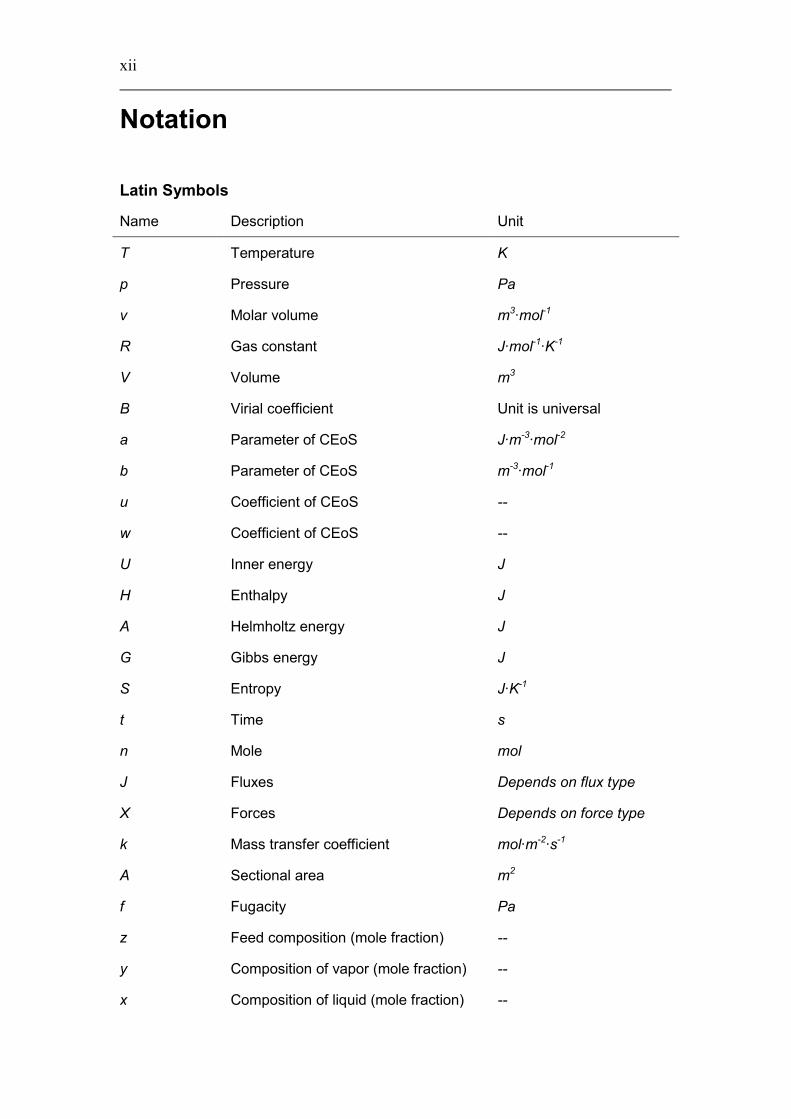
Notation
Latin Symbols
Name Description Unit
T Temperature K
p Pressure Pa
v Molar volume m3·mol-1
R Gas constant J·mol-1·K-1
V Volume m3
B Virial coefficient Unit is universal
a Parameter of CEoS J·m-3·mol-2
b Parameter of CEoS m-3·mol-1
u Coefficient of CEoS --
w Coefficient of CEoS --
U Inner energy J
H Enthalpy J
A Helmholtz energy J
G Gibbs energy J
S Entropy J·K-1
t Time s
n Mole mol
J Fluxes Depends on flux type
X Forces Depends on force type
k Mass transfer coefficient mol·m-2·s-1
A Sectional area m2
f Fugacity Pa
z Feed composition (mole fraction) --
y Composition of vapor (mole fraction) --
x Composition of liquid (mole fraction) --
xiii
Latin Symbols (continuous)
Name Description Unit
NC Number of components --
NP Number of total phases --
ic Component ID --
ip Phase ID --
φ Fugacity coefficient --
Z A parameter of CEoS, Z=pV/RT mol
A A parameter of CEoS, ap/(RT)2 --
B A parameter of CEoS, bp/(RT) --
C A function of CEoS --
ε A parameter of CEoS, A/B --
C A constant of mixing rule, C* --
q1 Parameter of mixing rule --
q2 Parameter of mixing rule --
q Variable of Exact mixing rule
U Variable of LPVP mixing rule mol-1
Greek Symbols
Name Description Unit
δ Parameter of mixing rule --
θ Phase partitioning coefficient --
µ Chemical potential J
υ Stoichiometric coefficient --
σ Rate of entropy production J·K-1·s-1
σ Component sink or source rate mol·s-1
xiv
Superscripts
Name Description Example
E Excess VE
( ) ID of phases (α),(k),(k�α)
tot total ntot
V Vapor phase fV
L1 1st liquid fL1
L2 2nd liquid fL2
L3 3rd liquid fL3
* A specific state C*
Subscripts
Name Description Example
i, j Components kij
2 Second Virial coefficient B2
3 Third Virial coefficient B3
s Entropy σs
ic Component ID σic
r Reaction σr
0 Initial state, t=0 n0
m Mixture property B2,m, φm
Abbreviations
Name Description
1PVDW One parameter VDW mixing rule
2PVDW Two parameter VDW mixing rule
BLCVM Modified LCVM mixing rule with second Virial coefficient
CEoS Cubic equation of state
CEoS/GE Mixing rule combining the CEoS and GE model
xv
Abbreviations (continuous)
Name Description
CHV2 Modified HV by adjusting the constant, 2nd version
CHV1 Modified HV by adjusting the constant, 1st version
COSMO Conductor-like screening model
CXLs CO2-expanded liquids
DFG German Research Foundation
EAL Mixing rule developed by Esmaeilzadeh, As’adi and Lashkarbolooki
EoS Equation of state
EPF Elementary Process Functions
Exact Mixing rule named by Kalospiros et al.
GE Excess Gibbs free energy model
HK Mixing rule developed by Heidemann and Kokal
HP High pressure
HV Huran-Vidal mixing rule
HVOS Modified HV by Orbey and Sandler mixing rule
HVLP Modified HV mixing rule with low pressure reference
HVT Modified HV mixing rule developed by Tochigi, et al.
IG Ideal gas model
ILs Ionic liquids
KTK Mixing rule developed by Kurihara, Tochigi and Kojima
LCSP Lower critical solution pressure
LCVM Linear combination of HV and MHV1 mixing rule
LLE Liquid-liquid equilibria
LLLE Liquid-liquid-liquid equilibria
LP Low pressure
LPVP Low pressure mixing rule employed vapor pressure standard state
MHV1 Modified HV with 1st order simplification mixing rule
MHV2 Modified HV with 2nd order simplification mixing rule
xvi
Abbreviations (continuous)
Name Description
MPR PR with modified α function
MSRK SRK with modified α function
MTC Modified Twu-Coon mixing rule
NRTL Non-Random Two Liquids model
ODE Ordinary differential equation
PC-SAFT Perturbed chain- statistical associating fluid theory
PR Peng-Robinson EoS
PRWS Peng-Robinson EoS with Wong-Sandler mixing rule
PSD Pressure-swing distillation
PSRK Predictive SRK mixing rule or model
Ref. Reference
RRE Rachford-Rice equation
scCO2 Supercritical CO2
SCF Supercritical fluids
Soave Mixing rule developed by Soave
SRK Soave-Redlich-Kwong EoS
TCO The original version of mixing rule developed by Twu and Coon
TCB(0) Modified TCO with pressure reference=0
TCB(r) Modified TCO with varied r
TPDF tangent plane distance function
TMS thermomorphic (or temperature-dependent) multi-component
solvent
UCSP Upper critical solution pressure
UNIFAC-PSRK Modified UNIFAC, version used in PSRK
UNIFAC-Lby Modified UNIFAC, Lyngby version
UNIFAC-Do Modified UNIFAC, Dortmund version
UNIQUAC Universal quasi chemical model
xvii
Abbreviations (continuous)
Name Description
USD U.S. dollar
Uniwaals An EoS developed by Gupte et al. 1986
VDW van der Waals mixing rule
VLE Vapor-liquid equilibria
VLLE Vapor-liquid-liquid equilibria
VOC Volatile Organic Compounds
Wilson Wilson activity coefficient model
WS Wong-Sandler mixing rule
Chemicals
Name Description
H2O Water
MeOH Methanol
EtOH Ethanol
1PrOH 1-propanol
2PrOH Isopropyl alcohol
1BuOH 1-butanol
MePOH 2-methyl-2-propanol
tBuOH Tert-butyl alcohol
DME Dimethyl ether
ACE Acetone
BUE 2-butanone
HAC Acetic acid
HPA Propionic acid
HBA Butyric acid
MeCN Acetonitrile
OCT 1-octene

xviii
Chemicals (continuous)
Name Description
NAL 1-nonanal
PhMe Toluene
DIOX 1,4-dioxane
THF Tetrahydrofuran
DMSO dimethyl sulfoxide
MeCE Methyl cyclohexane
PNE n-pentane
Ph Benzene
C6 Cyclohexane
EA Ethyl acetate
NBA n-butyl acetate
CO2 Carbon dioxide
CO Carbon monoxide
H2 Hydrogen
CH4 Methane
C2H4 Ethylene
C2H6 Ethane
C3H8 Propane
C4H10 Isobutane
CClF3 Trifluorochloromethane
CHF3 Trifluoromethane
1Do n-dodecene
C10 decane
NC13 1-dodecanal
OCT 1-octene
NAL 1-nonanal
Chapter 1
Introduction
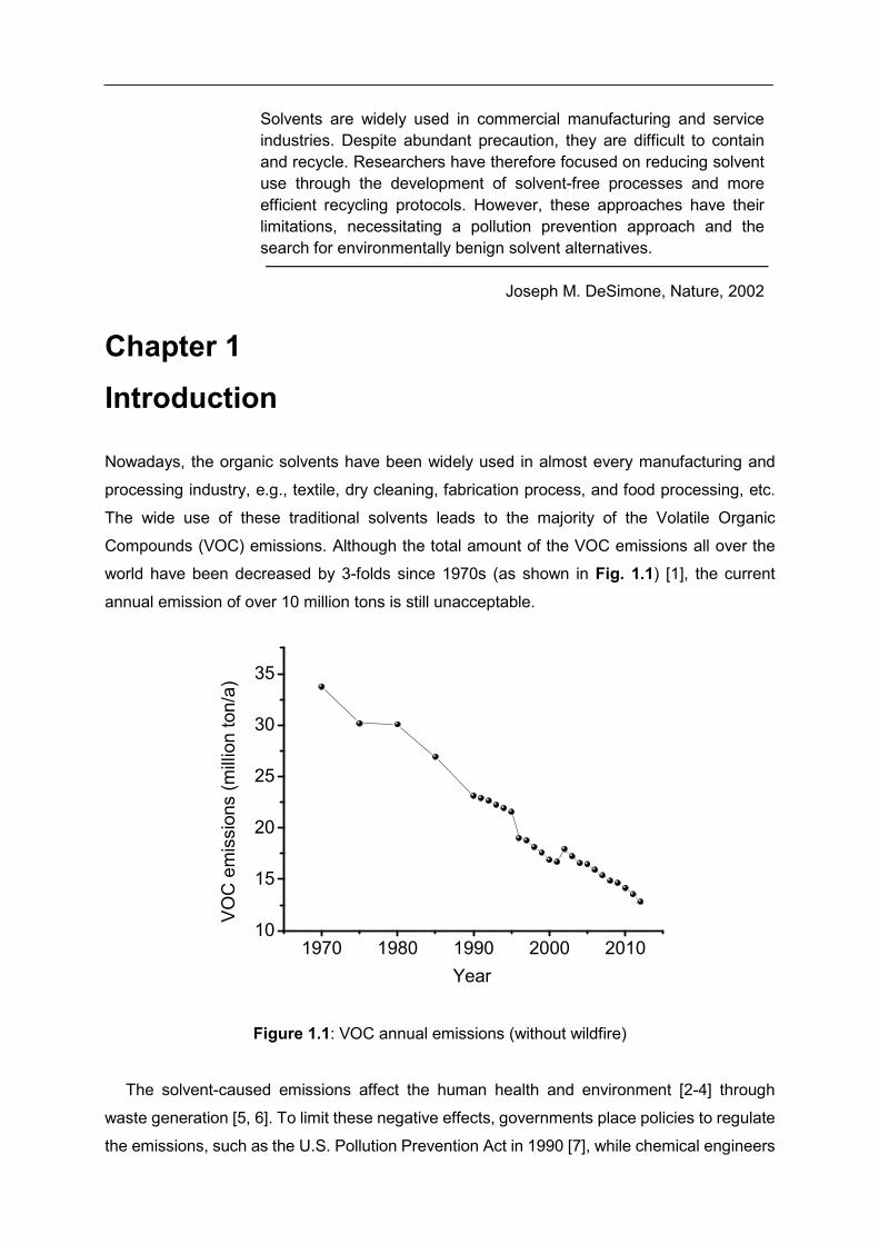
Nowadays, the organic solvents have been widely used in almost every manufacturing and
processing industry, e.g., textile, dry cleaning, fabrication process, and food processing, etc.
The wide use of these traditional solvents leads to the majority of the Volatile Organic
Compounds (VOC) emissions. Although the total amount of the VOC emissions all over the
world have been decreased by 3-folds since 1970s (as shown in Fig. 1.1) [1], the current
annual emission of over 10 million tons is still unacceptable.
Figure 1.1: VOC annual emissions (without wildfire)
The solvent-caused emissions affect the human health and environment [2-4] through
waste generation [5, 6]. To limit these negative effects, governments place policies to regulate
the emissions, such as the U.S. Pollution Prevention Act in 1990 [7], while chemical engineers
1970 1980 1990 2000 201010
15
20
25
30
35
VO
C e
mis
sio
ns (
mill
ion t
on/a
)
Year
Solvents are widely used in commercial manufacturing and service
industries. Despite abundant precaution, they are difficult to contain
and recycle. Researchers have therefore focused on reducing solvent
use through the development of solvent-free processes and more
efficient recycling protocols. However, these approaches have their
limitations, necessitating a pollution prevention approach and the
search for environmentally benign solvent alternatives.
Joseph M. DeSimone, Nature, 2002
2 Chapter 1 Introduction
search for new strategies to reduce the use of solvents, recycle the solvents, or design a
solvent-free process [8-12]. However, currently these strategies have their limitations, and
quite a number of instances of such processes have been shown to require process ‘liquid’ of
some kind [6]. Therefore, a new strategy using benign solvent alternatives would be more
attractive. The benign solvent alternatives are sorted in the following categories in accordance
with previous works [5, 6, 13, 14], i.e., supercritical fluids (SCF) [15-18], ionic liquids (ILs)
[19-22], fluorous phases [23-27], carbon dioxide (including supercritical CO2 (scCO2) and
CO2-expanded liquids (CXLs) [28-31]), and selected combinations of former benign solvent
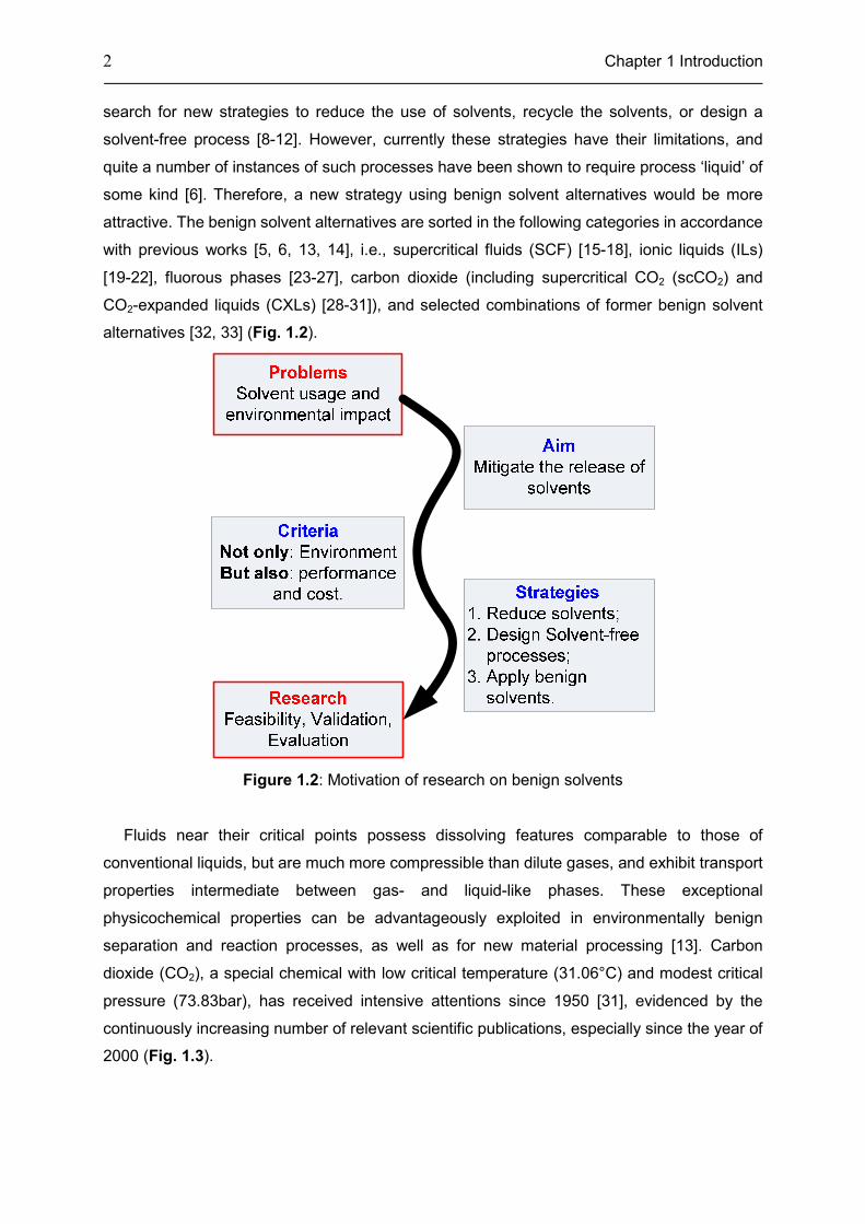
alternatives [32, 33] (Fig. 1.2).
Figure 1.2: Motivation of research on benign solvents
Fluids near their critical points possess dissolving features comparable to those of
conventional liquids, but are much more compressible than dilute gases, and exhibit transport
properties intermediate between gas- and liquid-like phases. These exceptional
physicochemical properties can be advantageously exploited in environmentally benign
separation and reaction processes, as well as for new material processing [13]. Carbon
dioxide (CO2), a special chemical with low critical temperature (31.06°C) and modest critical
pressure (73.83bar), has received intensive attentions since 1950 [31], evidenced by the
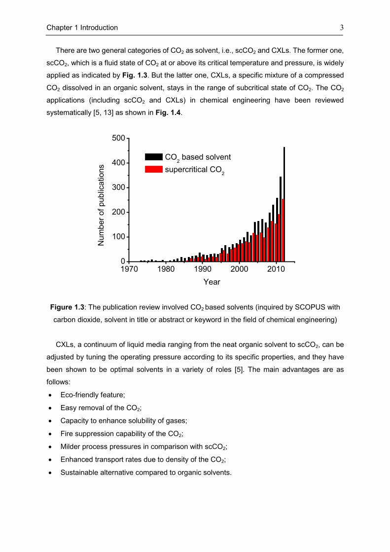
continuously increasing number of relevant scientific publications, especially since the year of
2000 (Fig. 1.3).
Chapter 1 Introduction 3
There are two general categories of CO2 as solvent, i.e., scCO2 and CXLs. The former one,
scCO2, which is a fluid state of CO2 at or above its critical temperature and pressure, is widely
applied as indicated by Fig. 1.3. But the latter one, CXLs, a specific mixture of a compressed
CO2 dissolved in an organic solvent, stays in the range of subcritical state of CO2. The CO2
applications (including scCO2 and CXLs) in chemical engineering have been reviewed
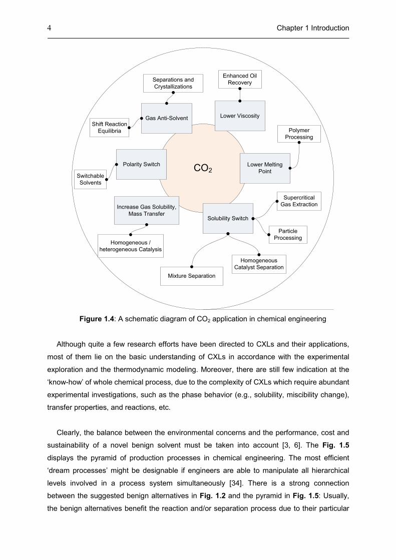
systematically [5, 13] as shown in Fig. 1.4.
Figure 1.3: The publication review involved CO2 based solvents (inquired by SCOPUS with
carbon dioxide, solvent in title or abstract or keyword in the field of chemical engineering)
CXLs, a continuum of liquid media ranging from the neat organic solvent to scCO2, can be
adjusted by tuning the operating pressure according to its specific properties, and they have
been shown to be optimal solvents in a variety of roles [5]. The main advantages are as
follows:
• Eco-friendly feature;
• Easy removal of the CO2;
• Capacity to enhance solubility of gases;
• Fire suppression capability of the CO2;
• Milder process pressures in comparison with scCO2;
• Enhanced transport rates due to density of the CO2;
• Sustainable alternative compared to organic solvents.
1970 1980 1990 2000 20100
100
200
300
400
500
Num
ber
of pub
lica
tions
Year
CO2 based solvent
supercritical CO2
4 Chapter 1 Introduction
Particle
Processing
Homogeneous
Catalyst Separation
Mixture Separation
CO2
Supercritical
Gas Extraction
Enhanced Oil
Recovery
Polymer
Processing
Separations and
Crystallizations
Homogeneous /
heterogeneous Catalysis
Lower Viscosity
Lower Melting
Point
Gas Anti-Solvent
Solubility Switch
Shift Reaction
Equilibria
Increase Gas Solubility,
Mass Transfer
Switchable
Solvents
Polarity Switch
Figure 1.4: A schematic diagram of CO2 application in chemical engineering
Although quite a few research efforts have been directed to CXLs and their applications,
most of them lie on the basic understanding of CXLs in accordance with the experimental
exploration and the thermodynamic modeling. Moreover, there are still few indication at the
‘know-how’ of whole chemical process, due to the complexity of CXLs which require abundant
experimental investigations, such as the phase behavior (e.g., solubility, miscibility change),
transfer properties, and reactions, etc.
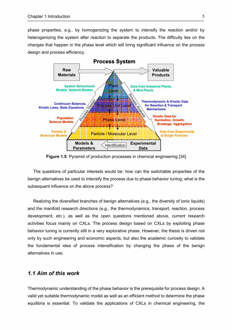
Clearly, the balance between the environmental concerns and the performance, cost and
sustainability of a novel benign solvent must be taken into account [3, 6]. The Fig. 1.5
displays the pyramid of production processes in chemical engineering. The most efficient
‘dream processes’ might be designable if engineers are able to manipulate all hierarchical
levels involved in a process system simultaneously [34]. There is a strong connection
between the suggested benign alternatives in Fig. 1.2 and the pyramid in Fig. 1.5: Usually,
the benign alternatives benefit the reaction and/or separation process due to their particular
Chapter 1 Introduction 5
phase properties, e.g., by homogenizing the system to intensify the reaction and/or by
heterogenizing the system after reaction to separate the products. The difficulty lies on the
changes that happen in the phase level which will bring significant influence on the process
design and process efficiency.
Figure 1.5: Pyramid of production processes in chemical engineering [34]
The questions of particular interests would be: how can the switchable properties of the
benign alternatives be used to intensify the process due to phase behavior tuning; what is the
subsequent influence on the above process?
Realizing the diversified branches of benign alternatives (e.g., the diversity of ionic liquids)
and the manifold research directions (e.g., the thermodynamics, transport, reaction, process
development, etc.), as well as the open questions mentioned above, current research
activities focus mainly on CXLs. The process design based on CXLs by exploiting phase
behavior tuning is currently still in a very explorative phase. However, the thesis is driven not
only by such engineering and economic aspects, but also the academic curiosity to validate
the fundamental idea of process intensification by changing the phase of the benign
alternatives in use.
1.1 Aim of this work
Thermodynamic understanding of the phase behavior is the prerequisite for process design. A
valid yet suitable thermodynamic model as well as an efficient method to determine the phase
equilibria is essential. To validate the applications of CXLs in chemical engineering, the
System Behavioural
Models, Network Models
Continuum Balances,
Kinetic Laws, State Equations
Experimental
Data
Models &
Parameters
Particle &
Molecular Models
Process Unit Level
Particle / Molecular Level
Data from Industrial Plants,
& Mini-Plants
Thermodynamic & Kinetic Data
for Reaction & Transport
Mechanisms
Phase LevelKinetic Data for
Nucleation, Growth,
Breakage, Aggregation
Raw
Materials
Data from Experiments
at Single Particles
Valuable
Products
Process A
nalysis
Pro
cess
Des
ign
Population
Balance Models
Plant
Level
Process System
Identification
6 Chapter 1 Introduction
thermodynamic phase behavior needs to be studied with priority. With clear understanding of
the phase behavior and efficient calculation, the goal of this work is thus to provide a share of
contribution to the designing of special processes based on CXLs, which are dependent on
and/or dominated by pressure variation. Hence, the following questions need to be answered:
• How to describe the phase behavior of CXLs? Would there be any model to predict the
phase behavior? If so, which one is the most suitable (i.e., simplest with satisfactory
accuracy)?
• How to determine the phase equilibria efficiently? Do we have any innovative method in
contrast to the conventional methods? If yes, what is it? Does it have physical sense?
How to validate it? What is the advantage from an engineering standpoint?
• What is the idea or concept of designing separation processes based on CXLs? What is
the difference from conventional solvent systems? How to realize it? Is it potentially
applicable? If yes, under which circumstances?
• Is the solubility of gas in gas liquid reactions so important? Can CXLs be used to enhance
reaction rate and selectivity? What kinds of exemplifications are interpreted? What
important information can be found to conduct further research?
There are other questions in the subject of CXLs which are not addressed in the scope of
this work. To clarify, these aspects are:
• scCO2 and other benign alternatives;
• Detailed experimental work to achieve phase equilibrium information. In this work, most
of phase behavior data are obtained from literature and project collaborators;
• The following methods to predict phase behavior, i.e., molecular simulation,
multi-parameter EoS (e.g., PC-SAFT) and COSMO, are not a topic of this thesis. The
reason is that the achievement of the parameters between/among the manifold
components involved in this thesis is extremely difficult;
• Process optimization and further process designing, such as process control and
apparatus, are not the main focus of this thesis.
1.2 This Thesis in a Nutshell
In this thesis, the general separation and reaction strategy by phase behavior tuning using
CXLs, detached from a particular system, stands in the foreground. To this end, phase
equilibria determination, including thermodynamic modeling and calculation method, is
demonstrated at the beginning; the further process design and analysis can then be possible
with such basis. In a sense, thermodynamics and the strategy by phase behavior tuning are
Chapter 1 Introduction 7
two threads in parallel in this thesis. With the final goal of process design and analysis,
thermodynamics provide an appropriate analytical method for particular systems.
Φ3→
α
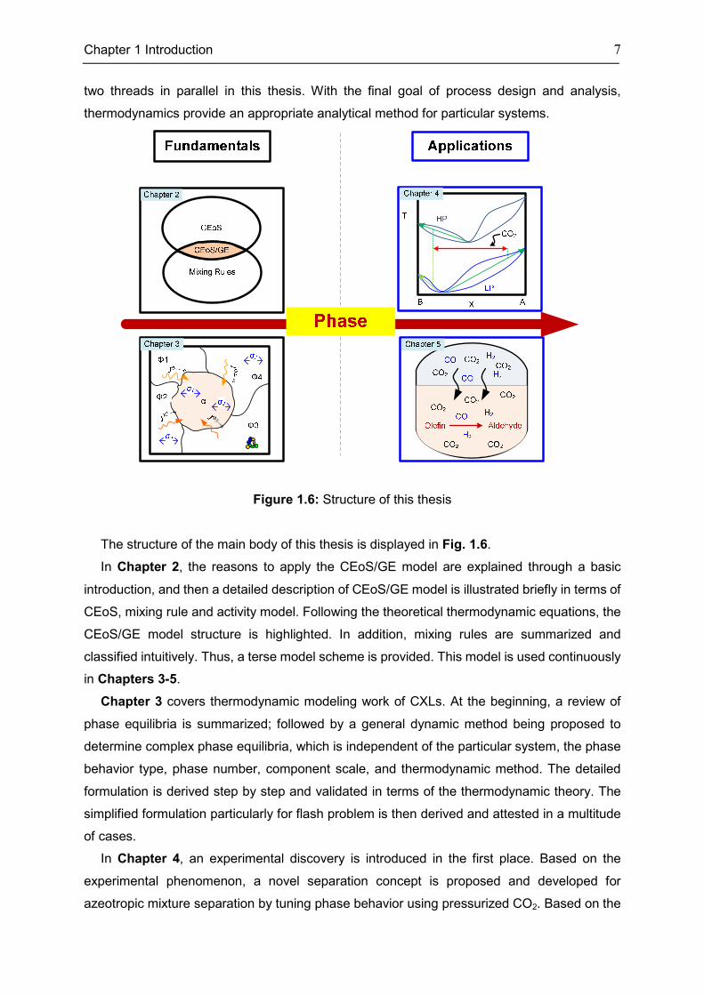
Figure 1.6: Structure of this thesis
The structure of the main body of this thesis is displayed in Fig. 1.6.
In Chapter 2, the reasons to apply the CEoS/GE model are explained through a basic
introduction, and then a detailed description of CEoS/GE model is illustrated briefly in terms of
CEoS, mixing rule and activity model. Following the theoretical thermodynamic equations, the
CEoS/GE model structure is highlighted. In addition, mixing rules are summarized and
classified intuitively. Thus, a terse model scheme is provided. This model is used continuously
in Chapters 3-5.
Chapter 3 covers thermodynamic modeling work of CXLs. At the beginning, a review of
phase equilibria is summarized; followed by a general dynamic method being proposed to
determine complex phase equilibria, which is independent of the particular system, the phase
behavior type, phase number, component scale, and thermodynamic method. The detailed
formulation is derived step by step and validated in terms of the thermodynamic theory. The
simplified formulation particularly for flash problem is then derived and attested in a multitude
of cases.
In Chapter 4, an experimental discovery is introduced in the first place. Based on the
experimental phenomenon, a novel separation concept is proposed and developed for
azeotropic mixture separation by tuning phase behavior using pressurized CO2. Based on the
8 Chapter 1 Introduction
concept, two process variants are put forward and validated using two classes of azeotropic
system, i.e., a pressure sensitive and asymmetric azeotropic system MeCN/H2O and a
pressure sensitive and symmetric azeotropic system DIOX/H2O. Finally, the performance of
the concept is evaluated in comparison with conventional separation technology, and the
feasibility of the new concept is categorized for different azeotropic systems.
In Chapter 5, the application of CXLs in reactions is reviewed briefly with the research of
CXLs for hydroformylation being emphasized in particular. The thermodynamic analysis is
highlighted to the level of understanding of components distribution for such reaction systems,
including the factors which can affect CXLs. Besides, a new ideal, CXTMS, is put forward and
the LLE phase behavior of 1-dodecene hydroformylation in TMS is modeled using
UNIFAC-Do.
Chapter 6 is the summary and conclusion section. The outlook on major topics, including
the experimental work, the predictive thermodynamic modeling, the hydroformylation and the
dynamic equations to determine phase equilibrium for open system, which may play a role in
future development, are also given.
The former two chapters (chapter 2 and chapter 3) are focusing on the fundamentals of the
phase thermodynamically and numerically. Based on the well-understanding the phase
identification, the latter two chapters (chapter 4 and chapter 5) are applying this knowledge to
the process concept. Therefore, they are tightly connected by the phase, and it is the golden
thread of this work.
Part I
Fundamentals
Chapter 2
Thermodynamic Modeling of CO2-Expanded
Liquids
Most industrial processes are designed for and operate near equilibrium conditions; even
when this is not the case, the knowledge of what would happen at equilibrium is often still
important [36]. Thermodynamics determines the principal feasibility of a process and often
allows an estimate of its operational costs, while kinetics give evidence about its technical
feasibility and its capital costs (e.g., reactor size). Therefore, before going to the unit level or
plant level, as shown in the pyramid of production processes in chemical engineering in
Chapter 1, the understanding of phase behavior of CXLs is very important, and it is the core
of this chapter. Furthermore, the design and development of the chemical process in this
thesis is based on the thermodynamic modeling work. Two types of phase behavior, i.e.,
vapor-liquid equilibria (VLE) and vapor-liquid-liquid equilibria (VLLE), are of particular interest.
Section 2.1 reviews phase behavior modeling using a fugacity coefficient approach within
elevated pressure; Section 2.2 highlights the performance of CEoS/GE modeling in terms of
several VLE systems; Section 2.3 displays prediction for several VLLE systems using
Peng-Robinson EoS with a Wong-Sandler mixing rule (PRWS).
2.1 Introduction
CXLs, especially CO2-expanded organic solvents, can dissolve large amount of CO2, whereby
every physical property of the mixture can be significantly changed [5]. The understanding of
such non-ideal behavior of CXLs is significantly important for chemical process design,
analysis, and optimization.
The most common approach to modeling the phase behavior of such non-ideal pressure
dependent systems is to use a fugacity-fugacity (φ-φ) approach [35-39]. Other methods, as
It is of special interest in chemistry and chemical engineering
because so many operations in the manufacture of chemical
products consist of phase contacting: V; an understanding of
any one of them is based, at least in part, on the science of
phase equilibrium.
John M. Prausnitz, et al.
Molecular Thermodynamics of Fluid-Phase Equilibria, 3rd ed.,
1999
Chapter 2 Thermodynamic Modeling of CXLs 11
reported by Mühlbauer and Ralal [38], are rarely applied for modeling CXLs, e.g., molecular
simulation can be used to model systems with only a few constituents [40-42]. The calculation
of the fugacity of each constituent in a mixture must include the equation-of-state (EoS) and
the mixing rule.
The EoS can be classified either as cubic equation-of-state (CEoS) or multi-parameter
equation-of-state (EoS). The CEoS, notably those by Soave-Redlich-Kwong (SRK) [43] and
Peng-Robinson (PR) [44] are real successful cases of applied thermodynamics in chemical
engineering. A multi-parameter EoS, which can probably offer higher accuracy, needs more
parameters that are sometimes not available. So its application is often not convenient. With
CEoS, the equation type is often less important than the mixing rules [35, 38], so special
attention must often be paid to the selection of appropriate mixing rules.
Mixing rules are quite diverse [38]. For simplicity, two types may be classified as reported
by Ghosh [39] and Adrian, et al. [35], namely mixing rules not incorporating excess Gibbs free
energy (GE) models and mixing rules incorporating GE models.
The first type of mixing rule includes the van der Waals mixing rule (VDW) and its
extensions [38]. A combination of CEoS and this first type have been employed to predict
several CXLs [45-51] but there are several drawbacks to using this combination. First, in
asymmetric systems prediction, VDW often fails to use constant kij (the adjustable interaction
parameters between component i and component j). For example, Ghosh, concluded that the
combination of VDW and CEoS cannot yield promising results for prediction of hydrocarbon
solubility in water [39]. Hence, for asymmetric, highly polar, and associating systems,
temperature and/or composition dependency must be implemented [35, 38, 39] in mixing
rules. However, most mixing rules of this type are empirical in integrating the temperature and
composition factors, and this may produce difficulties in modeling complex systems. Another
well-known drawback is that kij must be regressed from experimental data [37, 39, 52], which
requires reliable parameter estimation and time-consuming experimental work. Additionally,
the extrapolation of kij to a state beyond the experimental range is connected with uncertainty.
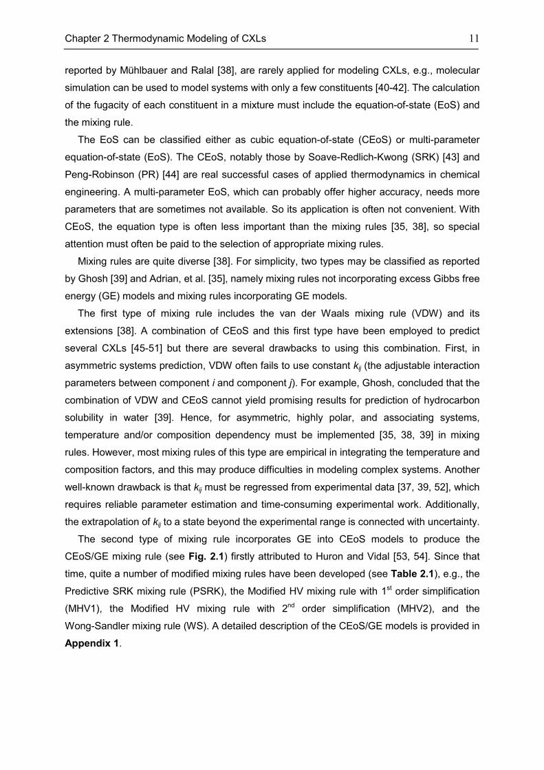
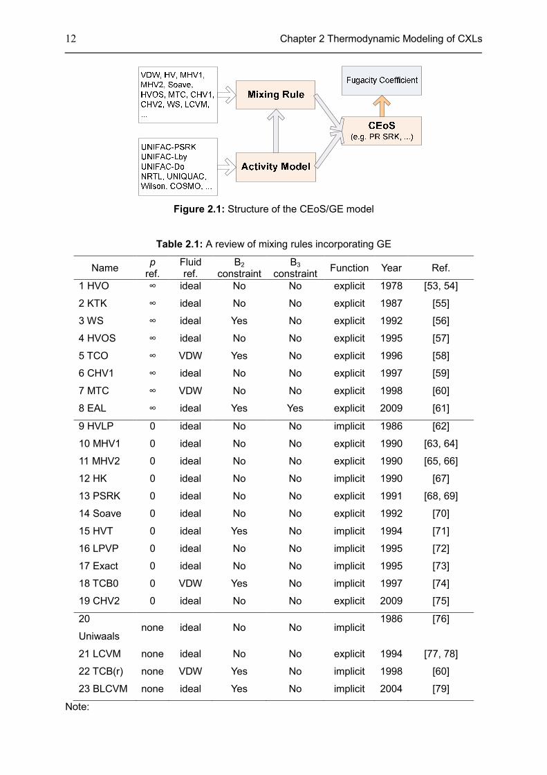
The second type of mixing rule incorporates GE into CEoS models to produce the
CEoS/GE mixing rule (see Fig. 2.1) firstly attributed to Huron and Vidal [53, 54]. Since that
time, quite a number of modified mixing rules have been developed (see Table 2.1), e.g., the
Predictive SRK mixing rule (PSRK), the Modified HV mixing rule with 1st order simplification
(MHV1), the Modified HV mixing rule with 2nd order simplification (MHV2), and the
Wong-Sandler mixing rule (WS). A detailed description of the CEoS/GE models is provided in
Appendix 1.
12 Chapter 2 Thermodynamic Modeling of CXLs
Figure 2.1: Structure of the CEoS/GE model
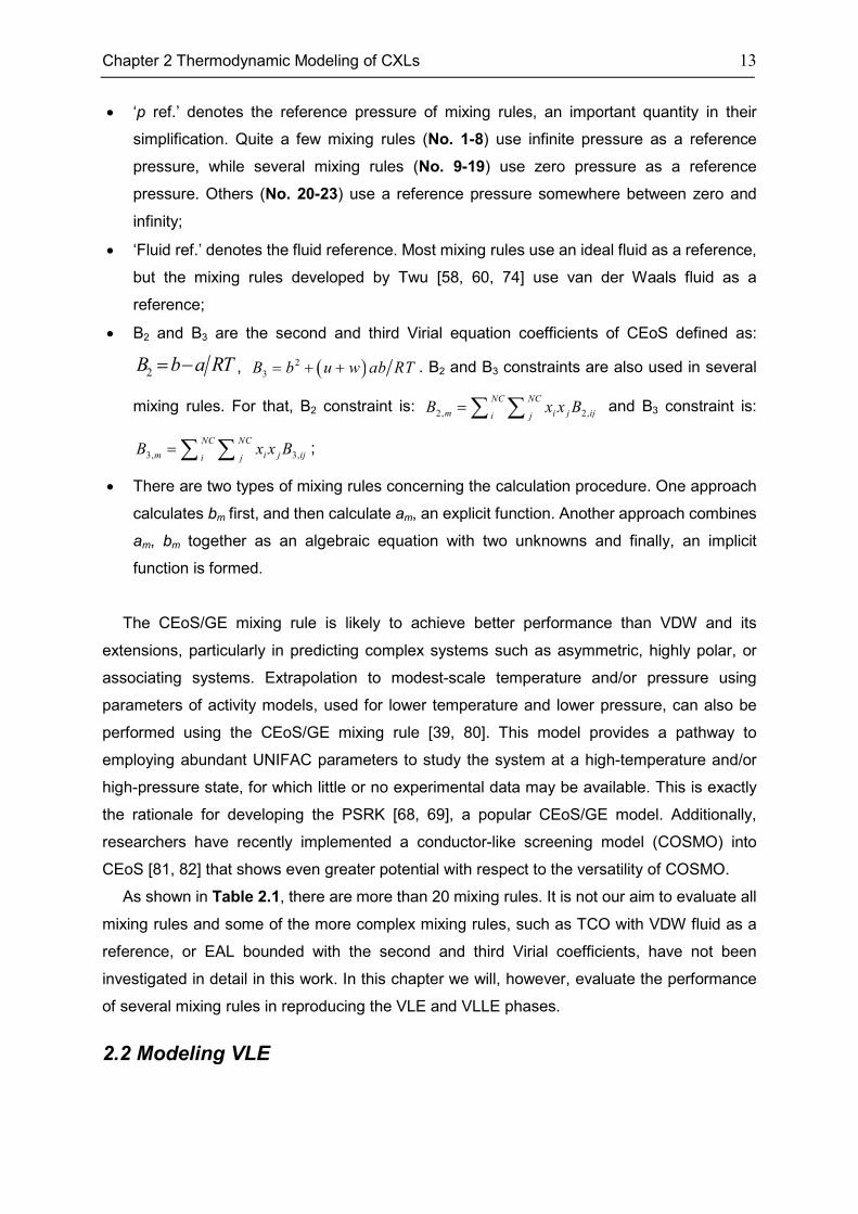
Table 2.1: A review of mixing rules incorporating GE
Name p
ref. Fluid ref.
B2 constraint
B3 constraint
Function Year Ref.
1 HVO ∞ ideal No No explicit 1978 [53, 54]
2 KTK ∞ ideal No No explicit 1987 [55]
3 WS ∞ ideal Yes No explicit 1992 [56]
4 HVOS ∞ ideal No No explicit 1995 [57]
5 TCO ∞ VDW Yes No explicit 1996 [58]
6 CHV1 ∞ ideal No No explicit 1997 [59]
7 MTC ∞ VDW No No explicit 1998 [60]
8 EAL ∞ ideal Yes Yes explicit 2009 [61]
9 HVLP 0 ideal No No implicit 1986 [62]
10 MHV1 0 ideal No No explicit 1990 [63, 64]
11 MHV2 0 ideal No No explicit 1990 [65, 66]
12 HK 0 ideal No No implicit 1990 [67]
13 PSRK 0 ideal No No explicit 1991 [68, 69]
14 Soave 0 ideal No No explicit 1992 [70]
15 HVT 0 ideal Yes No implicit 1994 [71]
16 LPVP 0 ideal No No implicit 1995 [72]
17 Exact 0 ideal No No implicit 1995 [73]
18 TCB0 0 VDW Yes No implicit 1997 [74]
19 CHV2 0 ideal No No explicit 2009 [75]
20
Uniwaals none ideal No No implicit
1986 [76]
21 LCVM none ideal No No explicit 1994 [77, 78]
22 TCB(r) none VDW Yes No implicit 1998 [60]
23 BLCVM none ideal Yes No implicit 2004 [79]
Note:
Chapter 2 Thermodynamic Modeling of CXLs 13
• ‘p ref.’ denotes the reference pressure of mixing rules, an important quantity in their
simplification. Quite a few mixing rules (No. 1-8) use infinite pressure as a reference
pressure, while several mixing rules (No. 9-19) use zero pressure as a reference
pressure. Others (No. 20-23) use a reference pressure somewhere between zero and
infinity;
• ‘Fluid ref.’ denotes the fluid reference. Most mixing rules use an ideal fluid as a reference,
but the mixing rules developed by Twu [58, 60, 74] use van der Waals fluid as a
reference;
• B2 and B3 are the second and third Virial equation coefficients of CEoS defined as:
2B b a RT= − , ( )2
3B b u w ab RT= + + . B2 and B3 constraints are also used in several
mixing rules. For that, B2 constraint is: 2, 2,
NC NC
m i j iji jB x x B=∑ ∑ and B3 constraint is:
3, 3,
NC NC
m i j iji jB x x B=∑ ∑ ;
• There are two types of mixing rules concerning the calculation procedure. One approach
calculates bm first, and then calculate am, an explicit function. Another approach combines
am, bm together as an algebraic equation with two unknowns and finally, an implicit
function is formed.
The CEoS/GE mixing rule is likely to achieve better performance than VDW and its
extensions, particularly in predicting complex systems such as asymmetric, highly polar, or
associating systems. Extrapolation to modest-scale temperature and/or pressure using
parameters of activity models, used for lower temperature and lower pressure, can also be
performed using the CEoS/GE mixing rule [39, 80]. This model provides a pathway to
employing abundant UNIFAC parameters to study the system at a high-temperature and/or
high-pressure state, for which little or no experimental data may be available. This is exactly
the rationale for developing the PSRK [68, 69], a popular CEoS/GE model. Additionally,
researchers have recently implemented a conductor-like screening model (COSMO) into
CEoS [81, 82] that shows even greater potential with respect to the versatility of COSMO.
As shown in Table 2.1, there are more than 20 mixing rules. It is not our aim to evaluate all
mixing rules and some of the more complex mixing rules, such as TCO with VDW fluid as a
reference, or EAL bounded with the second and third Virial coefficients, have not been
investigated in detail in this work. In this chapter we will, however, evaluate the performance
of several mixing rules in reproducing the VLE and VLLE phases.
2.2 Modeling VLE
14 Chapter 2 Thermodynamic Modeling of CXLs
22 VLE systems are modeled using several CEoS/GE models [52, 83] (Table 2.2), i.e., four
binary systems, 13 ternary systems, four quaternary systems, and one quinary system. The
modeling work covers four CEoS (PR, SRK, MPR, MSRK), 11 mixing rules (HVO, HVOS,
MTC, MHV1, MHV2, Soave, CHV2, LCVM, CHV1, WS, PSRK), and two versions of UNIFAC
(UNIFAC-Lby and UNIFAC-PSRK). The performance of the combination of CEoS and mixing
rule for the 1-octene hydroformylation reaction system is discussed in one of our publications
[52]. The detailed modeling work is given in Appendix 2. Several multicomponent VLE
systems studied in Chapter 3 (See Figs. A5.1-A5.4) are modeled by NRTL-IG model, a
necessary distinction.
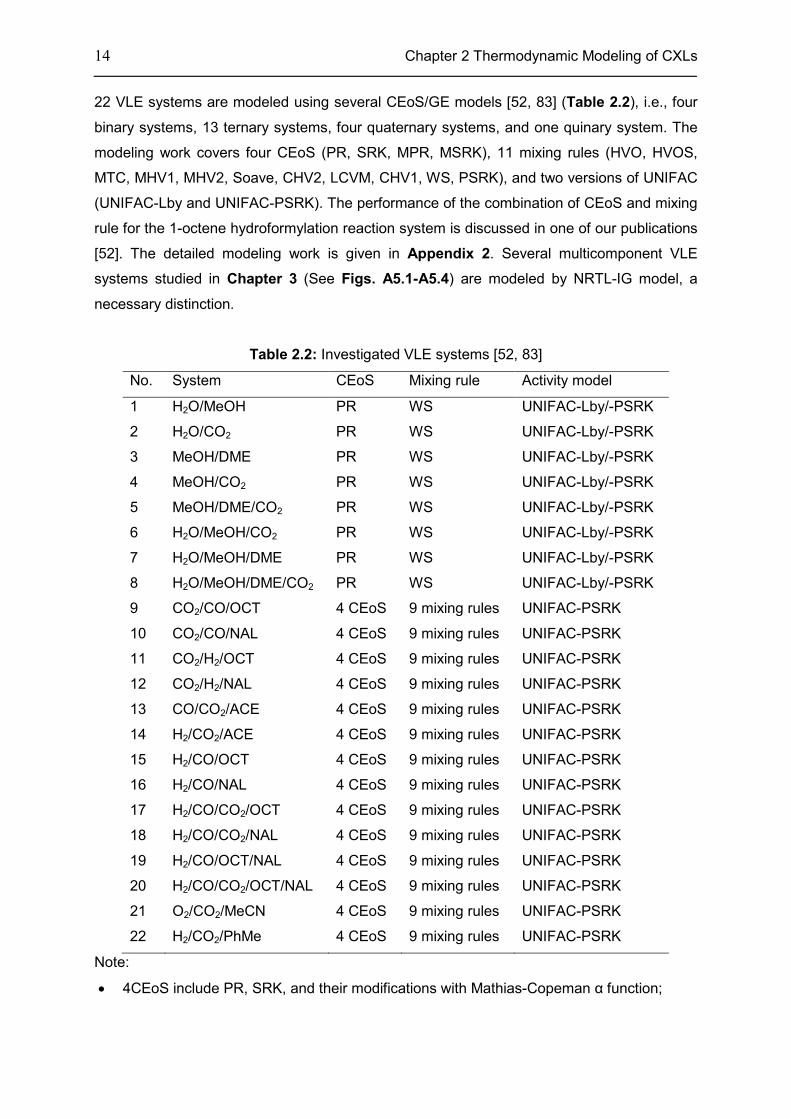
Table 2.2: Investigated VLE systems [52, 83]
No. System CEoS Mixing rule Activity model
1 H2O/MeOH PR WS UNIFAC-Lby/-PSRK
2 H2O/CO2 PR WS UNIFAC-Lby/-PSRK
3 MeOH/DME PR WS UNIFAC-Lby/-PSRK
4 MeOH/CO2 PR WS UNIFAC-Lby/-PSRK
5 MeOH/DME/CO2 PR WS UNIFAC-Lby/-PSRK
6 H2O/MeOH/CO2 PR WS UNIFAC-Lby/-PSRK
7 H2O/MeOH/DME PR WS UNIFAC-Lby/-PSRK
8 H2O/MeOH/DME/CO2 PR WS UNIFAC-Lby/-PSRK
9 CO2/CO/OCT 4 CEoS 9 mixing rules UNIFAC-PSRK
10 CO2/CO/NAL 4 CEoS 9 mixing rules UNIFAC-PSRK
11 CO2/H2/OCT 4 CEoS 9 mixing rules UNIFAC-PSRK
12 CO2/H2/NAL 4 CEoS 9 mixing rules UNIFAC-PSRK
13 CO/CO2/ACE 4 CEoS 9 mixing rules UNIFAC-PSRK
14 H2/CO2/ACE 4 CEoS 9 mixing rules UNIFAC-PSRK
15 H2/CO/OCT 4 CEoS 9 mixing rules UNIFAC-PSRK
16 H2/CO/NAL 4 CEoS 9 mixing rules UNIFAC-PSRK
17 H2/CO/CO2/OCT 4 CEoS 9 mixing rules UNIFAC-PSRK
18 H2/CO/CO2/NAL 4 CEoS 9 mixing rules UNIFAC-PSRK
19 H2/CO/OCT/NAL 4 CEoS 9 mixing rules UNIFAC-PSRK
20 H2/CO/CO2/OCT/NAL 4 CEoS 9 mixing rules UNIFAC-PSRK
21 O2/CO2/MeCN 4 CEoS 9 mixing rules UNIFAC-PSRK
22 H2/CO2/PhMe 4 CEoS 9 mixing rules UNIFAC-PSRK
Note:
• 4CEoS include PR, SRK, and their modifications with Mathias-Copeman α function;
Chapter 2 Thermodynamic Modeling of CXLs 15
• 9 mixing rules include HV, HVOS, MTC, MHV1, MHV2, Soave, CHV2, LCVM, and CHV1
(See Appendix 1).
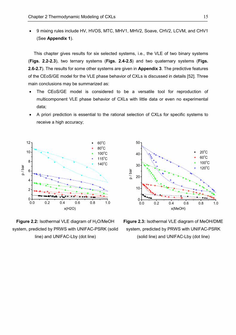
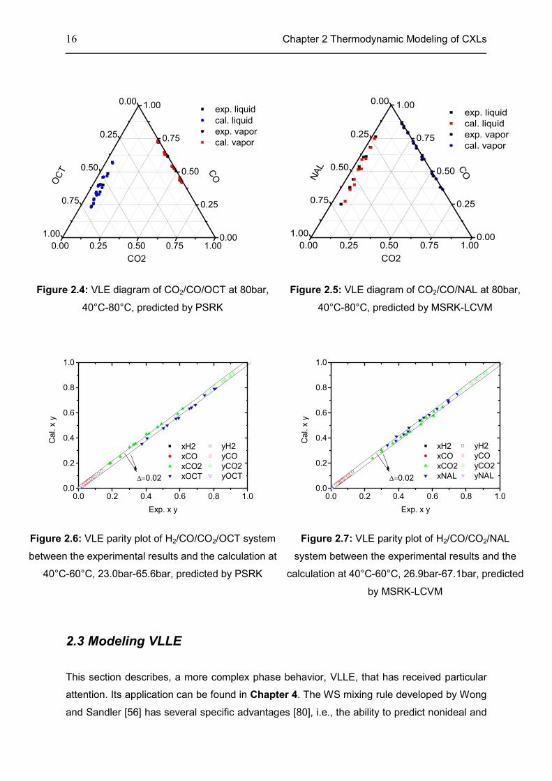
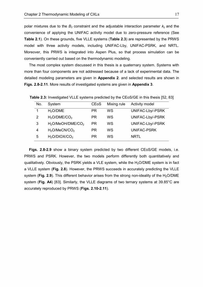
This chapter gives results for six selected systems, i.e., the VLE of two binary systems
(Figs. 2.2-2.3), two ternary systems (Figs. 2.4-2.5) and two quaternary systems (Figs.
2.6-2.7). The results for some other systems are given in Appendix 3. The predictive features
of the CEoS/GE model for the VLE phase behavior of CXLs is discussed in details [52]. Three
main conclusions may be summarized as:
• The CEoS/GE model is considered to be a versatile tool for reproduction of
multicomponent VLE phase behavior of CXLs with little data or even no experimental
data;
• A priori prediction is essential to the rational selection of CXLs for specific systems to
receive a high accuracy;
Figure 2.2: Isothermal VLE diagram of H2O/MeOH
system, predicted by PRWS with UNIFAC-PSRK (solid
line) and UNIFAC-Lby (dot line)
Figure 2.3: Isothermal VLE diagram of MeOH/DME
system, predicted by PRWS with UNIFAC-PSRK
(solid line) and UNIFAC-Lby (dot line)
0.0 0.2 0.4 0.6 0.8 1.00
2
4
6
8
10
12 60oC
80oC
100oC
115oC
140oC
p / b
ar
x(H2O)
0.0 0.2 0.4 0.6 0.8 1.00
10
20
30
40
50
20oC
60oC
100oC
120oC
p /
ba
r
x(MeOH)
16 Chapter 2 Thermodynamic Modeling of CXLs
Figure 2.4: VLE diagram of CO2/CO/OCT at 80bar,
40°C-80°C, predicted by PSRK
Figure 2.5: VLE diagram of CO2/CO/NAL at 80bar,
40°C-80°C, predicted by MSRK-LCVM
Figure 2.6: VLE parity plot of H2/CO/CO2/OCT system
between the experimental results and the calculation at
40°C-60°C, 23.0bar-65.6bar, predicted by PSRK
Figure 2.7: VLE parity plot of H2/CO/CO2/NAL
system between the experimental results and the
calculation at 40°C-60°C, 26.9bar-67.1bar, predicted
by MSRK-LCVM
2.3 Modeling VLLE
This section describes, a more complex phase behavior, VLLE, that has received particular
attention. Its application can be found in Chapter 4. The WS mixing rule developed by Wong
and Sandler [56] has several specific advantages [80], i.e., the ability to predict nonideal and
0.00 0.25 0.50 0.75 1.000.00
0.25
0.50
0.75
1.000.00
0.25
0.50
0.75
1.00
exp. liquid
cal. liquid
exp. vapor
cal. vapor
CO
OC
T
CO2
0.00 0.25 0.50 0.75 1.000.00
0.25
0.50
0.75
1.000.00
0.25
0.50
0.75
1.00
exp. liquid
cal. liquid
exp. vapor
cal. vapor
CO
NA
L
CO2
0.0 0.2 0.4 0.6 0.8 1.00.0
0.2
0.4
0.6
0.8
1.0
∆=0.02
xH2
xCO
xCO2
xOCT
Ca
l. x
y
Exp. x y
yH2
yCO
yCO2
yOCT
0.0 0.2 0.4 0.6 0.8 1.00.0
0.2
0.4
0.6
0.8
1.0
∆=0.02
xH2
xCO
xCO2
xNAL
Ca
l. x
y
Exp. x y
yH2
yCO
yCO2
yNAL
Chapter 2 Thermodynamic Modeling of CXLs 17
polar mixtures due to the B2 constraint and the adjustable interaction parameter kij and the
convenience of applying the UNIFAC activity model due to zero-pressure reference (See
Table 2.1). On these grounds, five VLLE systems (Table 2.3) are represented by the PRWS
model with three activity models, including UNIFAC-Lby, UNIFAC-PSRK, and NRTL.
Moreover, this PRWS is integrated into Aspen Plus, so that process simulation can be
conveniently carried out based on the thermodynamic modeling.
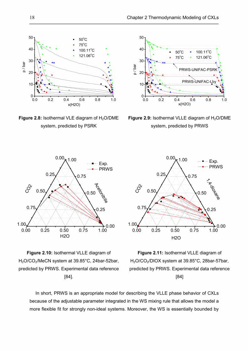
The most complex system discussed in this thesis is a quaternary system. Systems with
more than four components are not addressed because of a lack of experimental data. The
detailed modeling parameters are given in Appendix 2. and selected results are shown in
Figs. 2.8-2.11. More results of investigated systems are given in Appendix 3.
Table 2.3: Investigated VLLE systems predicted by the CEoS/GE in this thesis [52, 83]
No. System CEoS Mixing rule Activity model
1 H2O/DME PR WS UNIFAC-Lby/-PSRK
2 H2O/DME/CO2 PR WS UNIFAC-Lby/-PSRK
3 H2O/MeOH/DME/CO2 PR WS UNIFAC-Lby/-PSRK
4 H2O/MeCN/CO2 PR WS UNIFAC-PSRK
5 H2O/DIOX/CO2 PR WS NRTL
Figs. 2.8-2.9 show a binary system predicted by two different CEoS/GE models, i.e.
PRWS and PSRK. However, the two models perform differently both quantitatively and
qualitatively. Obviously, the PSRK yields a VLE system, while the H2O/DME system is in fact
a VLLE system (Fig. 2.8). However, the PRWS succeeds in accurately predicting the VLLE
system (Fig. 2.9). This different behavior arises from the strong non-ideality of the H2O/DME
system (Fig. A4) [83]. Similarly, the VLLE diagrams of two ternary systems at 39.85°C are
accurately reproduced by PRWS (Figs. 2.10-2.11).
18 Chapter 2 Thermodynamic Modeling of CXLs
Figure 2.8: Isothermal VLE diagram of H2O/DME
system, predicted by PSRK
Figure 2.9: Isothermal VLLE diagram of H2O/DME
system, predicted by PRWS
Figure 2.10: Isothermal VLLE diagram of
H2O/CO2/MeCN system at 39.85°C, 24bar-52bar,
predicted by PRWS. Experimental data reference
[84].
Figure 2.11: Isothermal VLLE diagram of
H2O/CO2/DIOX system at 39.85°C, 28bar-57bar,
predicted by PRWS. Experimental data reference
[84]
In short, PRWS is an appropriate model for describing the VLLE phase behavior of CXLs
because of the adjustable parameter integrated in the WS mixing rule that allows the model a
more flexible fit for strongly non-ideal systems. Moreover, the WS is essentially bounded by
0.0 0.2 0.4 0.6 0.8 1.00
10
20
30
40
50 50
oC
75oC
100.11oC
121.06oC
p / b
ar
x(H2O)
0.0 0.2 0.4 0.6 0.8 1.00
10
20
30
40
50
PRWS-UNIFAC-Lby
PRWS-UNIFAC-PSRK
100.11oC
121.06oC
50oC
75oC
p / b
ar
x(H2O)
0.00 0.25 0.50 0.75 1.000.00
0.25
0.50
0.75
1.000.00
0.25
0.50
0.75
1.00
Ace
tonitrile
Exp.
PRWS
CO
2
H2O
0.00 0.25 0.50 0.75 1.000.00
0.25
0.50
0.75
1.000.00
0.25
0.50
0.75
1.00
1,4
-dio
xane
Exp.
PRWS
CO
2
H2O
Chapter 2 Thermodynamic Modeling of CXLs 19
the second Virial coefficient (B2), producing better performance than mixing rules without such
constraints [56].
2.4 Chapter Summary
The CEoS/GE model succeeds in predicting the VLE phase behavior of CXLs, consistent with
results of earlier researches with respect to the performance of this model (see Section 2.1),
but also through our own validation for quite a number of multi-component systems. We find
that most of the CEoS/GE models accurately reproduce the VLE phase behavior of CXLs.
However, while not all CEoS/GE models can predict the VLLE phase behavior accurately,
in this work, PRWS succeeds in predicting the VLLE phase behavior of several systems. In
contrast, PSRK, sometimes recommended as a popular model for predicting the VLE phase
behavior of CXLs [52], fails to model the VLLE phase behavior of some systems, such as the
VLLE of systems involving DME and H2O.
The results presented in this chapter demonstrate the advantage of using UNIFAC. The
convenience of implementing UNIFAC into the CEoS/GE model provides a means for
predicting phase behavior in systems with little or no experimental data.
Chapter 3
Dynamic Determination of Phase Equilibria
In the previous chapter, the importance of phase equilibria to industrial processes is
emphasized and the thermodynamic models are used to predict the VLE and VLLE phase
behavior of CXLs systems. Another point regarding the field of the phase equilibria is the
question on how to determine the phase equilibria numerically in an efficient manner. This
knowledge is indispensable, especially for process simulation. Considering the complex
nature multiphase and multicomponent systems involved in this thesis (e.g., VLLE), an
efficient method to determine the phase equilibria is of particular importance. Therefore, the
main work of this chapter is on developing such an efficient approach to determine phase
equilibria. It has to be mentioned that this approach developed here is not only suitable for
calculating phase equilibria involved in this thesis, but also for other types of complex phase
equilibria.
With this purpose, a novel idea is proposed in the first place. The mass balance equations
are formulated based on the mass transfers among phases with respect to each constituent in
a closed system. The mass balance equations are derived according to the chemical potential
theory. As a result, a set of ODEs is formulated (dynamic equations) (Section 3.2). After that,
the new approach is evaluated by the universal criteria of phase equilibrium, which have been
developed in accordance with the second law of thermodynamics and dissipative
thermodynamics, and then this approach is exemplified by 17 systems with different phase
behaviors and thermodynamic methods (Section 3.3). Finally, the new approach towards two
engineering problems of phase behavior determination is discussed (Section 3.4). All results
show that the new approach is an efficient and powerful alternative for phase behavior
determination to conventional approaches.
Science has no final formulation. And it is moving away
from a static geometrical picture towards a description
in which evolution and history play essential roles.
Dilip Kondepudi
Modern Thermodynamics-From Heat Engines to
Dissipative Structures, 2004.
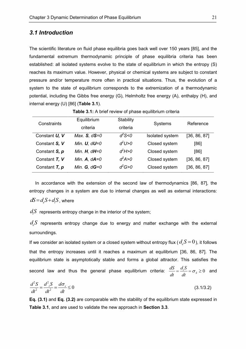
Chapter 3 Dynamic Determination of Phase Equilibrium 21
3.1 Introduction
The scientific literature on fluid phase equilibria goes back well over 150 years [85], and the
fundamental extremum thermodynamic principle of phase equilibria criteria has been
established: all isolated systems evolve to the state of equilibrium in which the entropy (S)
reaches its maximum value. However, physical or chemical systems are subject to constant
pressure and/or temperature more often in practical situations. Thus, the evolution of a
system to the state of equilibrium corresponds to the extremization of a thermodynamic
potential, including the Gibbs free energy (G), Helmholtz free energy (A), enthalpy (H), and
internal energy (U) [86] (Table 3.1).
Table 3.1: A brief review of phase equilibrium criteria
Constraints Equilibrium
criteria
Stability
criteria Systems Reference
Constant U, V Max. S, dS=0 d2S<0 Isolated system [36, 86, 87]
Constant S, V Min. U, dU=0 d2U>0 Closed system [86]
Constant S, p Min. H, dH=0 d2H>0 Closed system [86]
Constant T, V Min. A, dA=0 d2A>0 Closed system [36, 86, 87]
Constant T, p Min. G, dG=0 d2G>0 Closed system [36, 86, 87]
In accordance with the extension of the second law of thermodynamics [86, 87], the
entropy changes in a system are due to internal changes as well as external interactions:
e idS d S d S= + , where
id S represents entropy change in the interior of the system;
ed S represents entropy change due to energy and matter exchange with the external
surroundings.
If we consider an isolated system or a closed system without entropy flux ( 0ed S = ), it follows
that the entropy increases until it reaches a maximum at equilibrium [36, 86, 87]. The
equilibrium state is asymptotically stable and forms a global attractor. This satisfies the
second law and thus the general phase equilibrium criteria: 0iS
d SdS
dt dtσ= = ≥ and
22
2 20i sd S dd S
dt dt dt
σ= = ≤ (3.1/3.2)
Eq. (3.1) and Eq. (3.2) are comparable with the stability of the equilibrium state expressed in
Table 3.1, and are used to validate the new approach in Section 3.3.
22 Chapter 3 Dynamic Determination of Phase Equilibrium
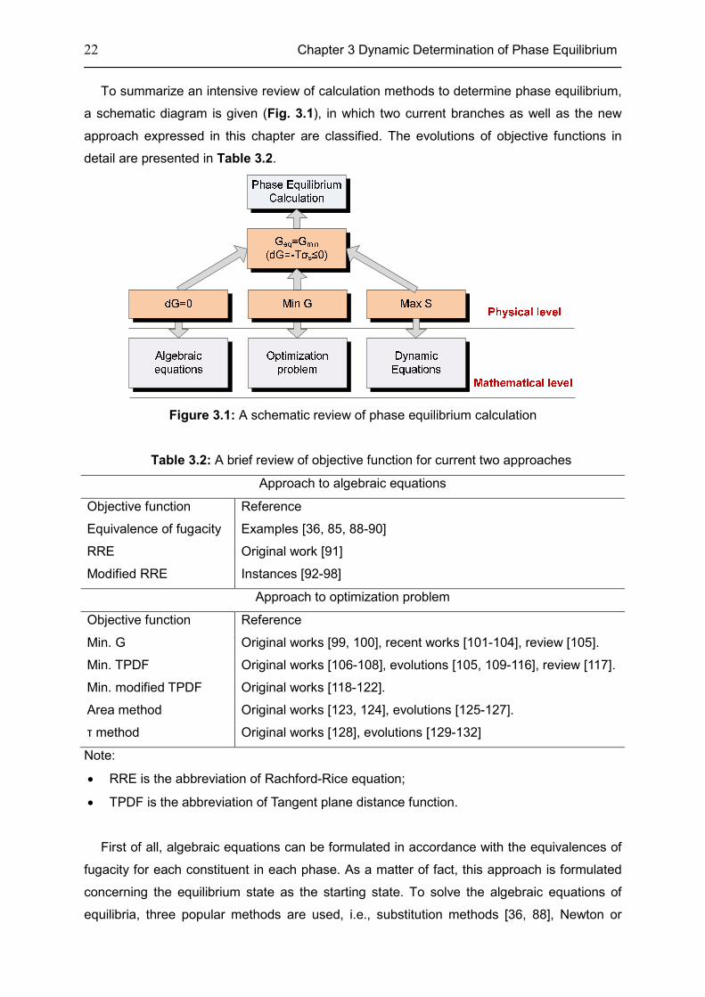
To summarize an intensive review of calculation methods to determine phase equilibrium,
a schematic diagram is given (Fig. 3.1), in which two current branches as well as the new
approach expressed in this chapter are classified. The evolutions of objective functions in
detail are presented in Table 3.2.
Figure 3.1: A schematic review of phase equilibrium calculation
Table 3.2: A brief review of objective function for current two approaches
Approach to algebraic equations
Objective function Reference
Equivalence of fugacity Examples [36, 85, 88-90]
RRE Original work [91]
Modified RRE Instances [92-98]
Approach to optimization problem
Objective function Reference
Min. G Original works [99, 100], recent works [101-104], review [105].
Min. TPDF Original works [106-108], evolutions [105, 109-116], review [117].
Min. modified TPDF Original works [118-122].
Area method Original works [123, 124], evolutions [125-127].
τ method Original works [128], evolutions [129-132]
Note:
• RRE is the abbreviation of Rachford-Rice equation;
• TPDF is the abbreviation of Tangent plane distance function.
First of all, algebraic equations can be formulated in accordance with the equivalences of
fugacity for each constituent in each phase. As a matter of fact, this approach is formulated
concerning the equilibrium state as the starting state. To solve the algebraic equations of
equilibria, three popular methods are used, i.e., substitution methods [36, 88], Newton or
Chapter 3 Dynamic Determination of Phase Equilibrium 23
Quasi-Newton methods [95-98, 133] (see review [102]), and homotopy continuation method
[117, 134-138] (see review [139, 140]). However, as an illustration, although the direct
substitution method converges fast, this method is limited and can only be used for calculating
simple ideal systems, where the fugacity coefficients are only weakly dependent on the phase
composition [108]. The application of the Newton method and Newton based methods is
limited due to the critical requirements that the initialization must be close enough to the
solution.
In contrast to the algebraic equations, another approach starts from non-equilibrium state.
As a consequence, an objective function is minimized, i.e., minimum G, minimum TPDF,
minimum modified TPDF, maximum Gibbs free energy surface integration (also named area
method) and τ method. On the whole, the minimum Gibbs free energy and the minimum
TPDF are the most popular two, and they are a necessary and sufficient condition for the
phase equilibrium. Other objective functions have downsides. For example, in spite of several
derivations of minimum modified TPDF, they are applied rarely. Whereas, for the area method
and the τ method, there is no guarantee to prove that they are necessary and sufficient
conditions for phase equilibrium. With the goal to find the optimal solutions, A variety of
optimization methods can be employed. For that, Kangas has classified two global methods,
i.e., stochastic optimization methods and global deterministic optimization methods [117].
Steyer et al. [141] used a rate-based approach to determine liquid-liquid equilibrium (LLE),
which starts also from non-equilibrium state. Through four cases, the high efficiency of the
approach is confirmed in comparison with homotopy. However, the approach cannot be used
to determine other phase behaviors apart from LLE, and the work did not attest the necessary
and sufficient conditions of phase equilibrium of this approach.
Quite a number of popular methods for calculating phase equilibrium still face challenges
when used for solving engineering problems.
• The first challenge comes from intrinsic thermodynamic models themselves. Most of the
models applied regressed parameters from pure components, binary mixtures or low
scale multicomponent mixtures and there is great uncertainty when employing these
parameters with specific mixtures [114]. Moreover, the models have non-uniqueness of
minima and maxima in the Gibbs energy surface, which is directly used to determine
thermodynamically stable, metastable and unstable equilibrium states [142]. Therefore,
the objective function consists in the highly non-linear and non-convex form, which gives
no rigorous guarantee that the global minimum will be found [101, 109, 111];
• The second challenge comes from the prior determination of the number of phases [105,
113, 131, 142]. Usually a small number of phases are assumed. If they are not stable,
phases will be split adding a new phase to reformulate the mathematical objective
24 Chapter 3 Dynamic Determination of Phase Equilibrium
function and the phase equilibrium calculation is repeated. This process continues until
the appropriate number of phases is found. The phase equilibrium can then be identified
numerically. However, if too many phases are assumed, numerical problems may arise,
or cause the solution to converge to a trivial or local extrema [105, 113, 131].
• The third challenge regards the numerical difficulties encountered using numerical
techniques [114, 142], which sometimes are very complex.
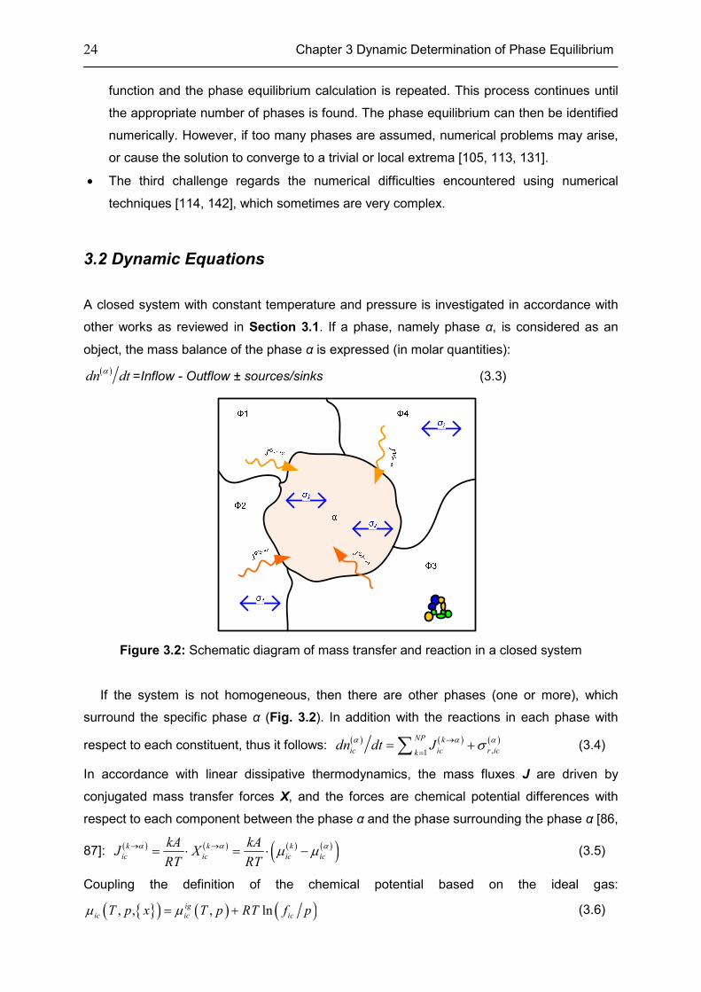
3.2 Dynamic Equations
A closed system with constant temperature and pressure is investigated in accordance with
other works as reviewed in Section 3.1. If a phase, namely phase α, is considered as an
object, the mass balance of the phase α is expressed (in molar quantities):
( )dn dtα
=Inflow - Outflow ± sources/sinks (3.3)
Figure 3.2: Schematic diagram of mass transfer and reaction in a closed system
If the system is not homogeneous, then there are other phases (one or more), which
surround the specific phase α (Fig. 3.2). In addition with the reactions in each phase with
respect to each constituent, thus it follows: ( ) ( ) ( )
,1
NP k
ic ic r ickdn dt J
α α ασ→
== +∑ (3.4)
In accordance with linear dissipative thermodynamics, the mass fluxes J are driven by
conjugated mass transfer forces X, and the forces are chemical potential differences with
respect to each component between the phase α and the phase surrounding the phase α [86,
87]: ( ) ( ) ( ) ( )( )k k k
ic ic ic ic
kA kAJ X
RT RT
α α αµ µ→ →= ⋅ = ⋅ − (3.5)
Coupling the definition of the chemical potential based on the ideal gas:
{ }( ) ( ) ( ), , , lnig
ic ic icT p x T p RT f pµ µ= + (3.6)
Chapter 3 Dynamic Determination of Phase Equilibrium 25
With regard to eqs. (3.5) (3.6), the eq. (3.4) is derived as:
( )
( ) ( )1( ) ( )
,
1,
lnNP
NPkic
ic ic r ic
k k
dnkA f f
dt
ααα
α
σ−
= ≠
= +
∏ (3.7)
This equation is a schematic equation, which figures out the relationship of each component
in a specific phase and fugacity of the component in all phases. The meaning of the symbols
expressed above is listed here.
( )icnα
stands for the mole of constituent ic in the phase α;
( )k
icJα→
stands for the flux from phase k to phase α with respect to component ic;
( ),r ic
ασ stands for the source or sinks with respect to component ic in the phase α.
( )k
icXα→
stands for the force from phase k to phase α with respect to component ic;
( )k
icµ stands for the chemical potential of the constituent ic in phase k;
kA stands for the product term of mass transfer coefficient k and the
interfacial area A ;
{ }( ), ,ic T p xµ stands for the chemical potential of a mixture under T, p condition with
composition { }x ;
( ),ig
ic T pµ stands for the chemical potential of a pure ideal gas under T, p condition;
( )k
icf stands for the fugacity of the constituent ic of mixture in phase k, which is a
function of { }, ,T p x ;
1,
NP
k k α= ≠∏ k is phase ID, which counts from 1 to NP, but k cannot be equal to α;
A closed system without any reactions is the specific interest of this thesis. Therefore, the
eq. (3.7) is simplified as:
( )
( ) 1( ) ( )
1,
lnNP
NPkic
ic ic
k k
dnkA f f
dt
αα
α
−
= ≠
=
∏ (3.8)
However, the eq. (3.8) cannot to be solved directly, because the number of equations is
less than the number of unknowns ({ } { },x n ). There are NC*NP equations, whereas, the
unknowns are 2NC*NP. For this reason, the number of unknowns has to be reduced.
Here ( )ic
αθ , which denotes the phase partitioning coefficient of the constituent ic in the fluid
phase α with respect to all constituents, is implemented. With regard to the definition of ( )ic
αθ ,
it follows: ( ) ( ) tot
ic ic icn nα αθ = ,
( )1
1NF k
ickθ
==∑ and ( ) ( ) tot
ic ic icn nα αθ= ⋅ (3.9)
Since the reaction is not involved here, so tot tot tot
ic icn n z= ⋅ , and ( ) ( ) tot tot
ic ic icn n zα αθ= ⋅ ⋅ (3.10)
26 Chapter 3 Dynamic Determination of Phase Equilibrium
It follows ( ) ( ) ( ) ( ) ( )( )1 1
NC NCtot tot
ic ic ic ic ic ic icic icx n n z zα α α α αθ θ
= == = ⋅ ⋅∑ ∑ (3.11)
Thus, the relationship among { }θ , { }x and { }n can be established concerning the eqs.
(3.9-3.11). The unknowns ({ } { },x n ) are replaced by the new unknowns { }θ . In this way, the
number of unknowns is reduced to a value equal to the number of equations. Consequently,
the dynamic equations can be solved in principle.
Inserting the eq. (3.10) into eq. (3.8), an equation is yielded:
( )
( ) 1( ) ( )
1,
lnNP
NPkic
ic ictot totk kic
d kAf f
dt n z
αα
α
θ −
= ≠
= ⋅
∏
(3.12)
These are the dynamic equations which cover a closed system without any reactions, and
they are used to determine the most practical phase behaviors in the field of chemical
engineering in this thesis, i.e., VLE, LLE, VLLE and LLLE. The calculation of solid solubility is
not particular interest, because the scale of the mathematical equation (e.g., SLE) is only one
and current methods, e.g., Newton method, can handle it efficiently. Therefore, the
development of a specific approach is not necessary. Moreover, two facets are summarized
for the calculation in detail.
• Firstly, the reduction of the scale of the ordinary differential equations (ODEs) is
reasonable in accordance with ( )
11
NF k
ickθ
==∑ . Thereby, only NP-1 fluid phases are
investigated with regard to the ( )k
icθ ;
• Secondly, several parameters can be fixed as constant values. For example, 1totn = .
Similarly, the value of k and A is set as 1 in this thesis, because they do not affect stable
solutions once ODEs reach equilibrium state in principle, but just affect the calculation
time to approach the steady-state. However, they cannot be too large or too small;
otherwise, the ODEs will be stiff if kA is too large or the calculation needs a long time if kA
is too small.
Here are several detailed equations for calculating the phase equilibria of VLE, VLLE, LLE,
and LLLE in this thesis (Table 3.3).
Table 3.3: Dynamic equations for calculating the phase equilibria
Type Investigated phases Simplified dynamic equation
VLE Liquid ( )lnL V L tot
ic ic ic icd dt f f zθ =
Chapter 3 Dynamic Determination of Phase Equilibrium 27
LLE One liquid ( )2 1 2lnL L L tot
ic ic ic icd dt f f zθ =
VLLE Two liquid phases
( )
( )
21 2 1
22 1 2
ln
ln
L V L L tot
ic ic ic ic ic
L V L L tot
ic ic ic ic ic
d dt f f f z
d dt f f f z
θ
θ
= ⋅
= ⋅
LLLE Two liquid phases
( )
( )
21 3 2 1
22 3 1 2
ln
ln
L L L L tot
ic ic ic ic ic
L L L L tot
ic ic ic ic ic
d dt f f f z
d dt f f f z
θ
θ
= ⋅
= ⋅
Note:
• The fugacity of vapor (or gas) phase is usually calculated using this equation:
V V
i if p ϕ= ⋅ , V
iϕ denotes the fugacity coefficient of component i in the vapor phase;
• The fugacity of liquid phase(s) is usually calculated either using this equation:
L L
i if p ϕ= ⋅ or using activity coefficient: V s
i i i if p x γ= ⋅ ⋅ , here s
ip denotes the
saturated pressure of component i and iγ denotes the activity coefficient of
component i.
3.3 Validation and Evaluation
The previous section has formulated the dynamic equations, whereas, in this section, the
validation of the dynamic equations will be discussed using results collected from 17
examples, which cover different multicomponent, multiphase and different thermodynamic
methods.
The 17 cases presented in Table 3.4 are shown in more detail in Table A4.1, Appendix 4.
It clearly shows that the investigated instances in this thesis cover the phase behaviors from
low component scale to high component scale. Only two cases are discussed as
representatives in this section to avoid repetition. It is well-known that if the system is not ideal
when it contains more than one liquid phase, such as in LLE, VLLE, LLLE, etc. systems. The
equilibrium phase behaviors for two complex cases are depicted in Fig. 3.3 and Fig. 3.4 in
which phase behavior calculations are usually extremely difficult to solve owing to the highly
non-ideal behavior. Random initial values were generated for these two systems. More results
are presented in Table A4.2, the consistency of all calculated results for all investigated
systems confirms the feasibility of the dynamic equations to determine the phase equilibria.
28 Chapter 3 Dynamic Determination of Phase Equilibrium
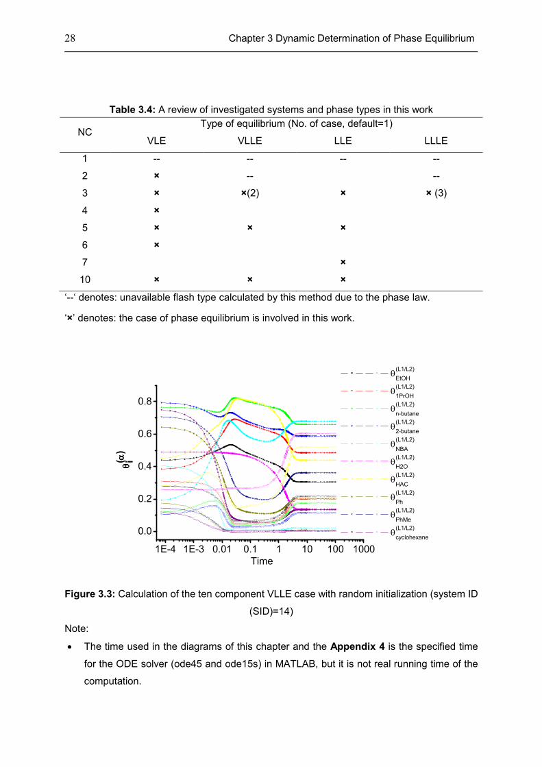
Table 3.4: A review of investigated systems and phase types in this work
NC Type of equilibrium (No. of case, default=1)
VLE VLLE LLE LLLE
1 -- -- -- --
2 × -- --
3 × ×(2) × × (3)
4 ×
5 × × ×
6 ×
7 ×
10 × × ×
‘--‘ denotes: unavailable flash type calculated by this method due to the phase law.
‘×’ denotes: the case of phase equilibrium is involved in this work.
Figure 3.3: Calculation of the ten component VLLE case with random initialization (system ID
(SID)=14)
Note:
• The time used in the diagrams of this chapter and the Appendix 4 is the specified time
for the ODE solver (ode45 and ode15s) in MATLAB, but it is not real running time of the
computation.
1E-4 1E-3 0.01 0.1 1 10 100 1000
0.0
0.2
0.4
0.6
0.8
θ(L1/L2)
EtOH
θ(L1/L2)
1PrOH
θ(L1/L2)
n-butane
θ(L1/L2)
2-butane
θ(L1/L2)
NBA
θ(L1/L2)
H2O
θ(L1/L2)
HAC
θ(L1/L2)
Ph
θ(L1/L2)
PhMe
θ(L1/L2)
cyclohexane
Time
θθ θθ( αα αα)
i
Chapter 3 Dynamic Determination of Phase Equilibrium 29
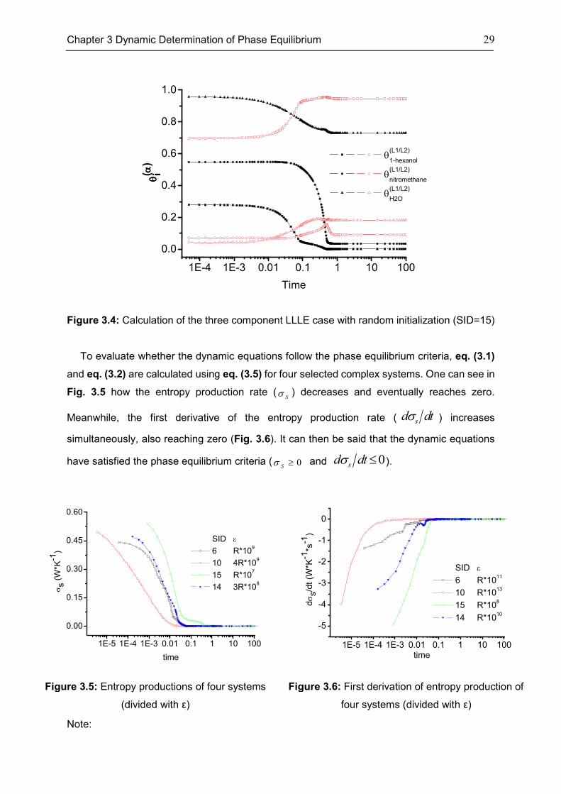
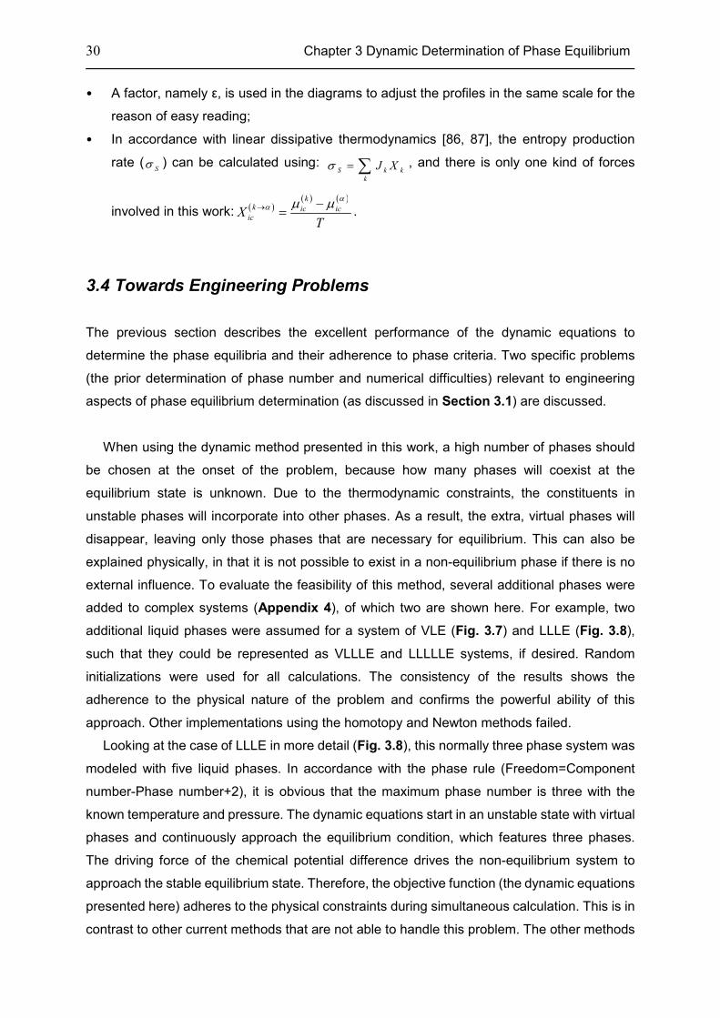
Figure 3.4: Calculation of the three component LLLE case with random initialization (SID=15)
To evaluate whether the dynamic equations follow the phase equilibrium criteria, eq. (3.1)
and eq. (3.2) are calculated using eq. (3.5) for four selected complex systems. One can see in
Fig. 3.5 how the entropy production rate (Sσ ) decreases and eventually reaches zero.
Meanwhile, the first derivative of the entropy production rate ( σsd dt ) increases
simultaneously, also reaching zero (Fig. 3.6). It can then be said that the dynamic equations
have satisfied the phase equilibrium criteria ( 0Sσ ≥ and 0σ ≤sd dt ).
Figure 3.5: Entropy productions of four systems
(divided with ε)
Figure 3.6: First derivation of entropy production of
four systems (divided with ε)
Note:
1E-4 1E-3 0.01 0.1 1 10 100
0.0
0.2
0.4
0.6
0.8
1.0
θθ θθ( αα αα)
i
Time
θ(L1/L2)
1-hexanol
θ(L1/L2)
nitromethane
θ(L1/L2)
H2O
1E-5 1E-4 1E-3 0.01 0.1 1 10 100
0.00
0.15
0.30
0.45
0.60
SID ε
6 R*109
10 4R*109
15 R*107
14 3R*108
σs (
W*K
-1)
time
1E-5 1E-4 1E-3 0.01 0.1 1 10 100
-5
-4
-3
-2
-1
0
dσ
s/d
t (W
*K-1
*s-1
)
time
SID ε
6 R*1011
10 R*1013
15 R*108
14 R*1010
30 Chapter 3 Dynamic Determination of Phase Equilibrium
• A factor, namely ε, is used in the diagrams to adjust the profiles in the same scale for the
reason of easy reading;
• In accordance with linear dissipative thermodynamics [86, 87], the entropy production
rate (Sσ ) can be calculated using:
S k k
k
J Xσ = ∑ , and there is only one kind of forces
involved in this work: ( )( ) ( )k
k ic icic
XT
αα µ µ→ −= .
3.4 Towards Engineering Problems
The previous section describes the excellent performance of the dynamic equations to
determine the phase equilibria and their adherence to phase criteria. Two specific problems
(the prior determination of phase number and numerical difficulties) relevant to engineering
aspects of phase equilibrium determination (as discussed in Section 3.1) are discussed.
When using the dynamic method presented in this work, a high number of phases should
be chosen at the onset of the problem, because how many phases will coexist at the
equilibrium state is unknown. Due to the thermodynamic constraints, the constituents in
unstable phases will incorporate into other phases. As a result, the extra, virtual phases will
disappear, leaving only those phases that are necessary for equilibrium. This can also be
explained physically, in that it is not possible to exist in a non-equilibrium phase if there is no
external influence. To evaluate the feasibility of this method, several additional phases were
added to complex systems (Appendix 4), of which two are shown here. For example, two
additional liquid phases were assumed for a system of VLE (Fig. 3.7) and LLLE (Fig. 3.8),
such that they could be represented as VLLLE and LLLLLE systems, if desired. Random
initializations were used for all calculations. The consistency of the results shows the
adherence to the physical nature of the problem and confirms the powerful ability of this
approach. Other implementations using the homotopy and Newton methods failed.
Looking at the case of LLLE in more detail (Fig. 3.8), this normally three phase system was
modeled with five liquid phases. In accordance with the phase rule (Freedom=Component
number-Phase number+2), it is obvious that the maximum phase number is three with the
known temperature and pressure. The dynamic equations start in an unstable state with virtual
phases and continuously approach the equilibrium condition, which features three phases.
The driving force of the chemical potential difference drives the non-equilibrium system to
approach the stable equilibrium state. Therefore, the objective function (the dynamic equations
presented here) adheres to the physical constraints during simultaneous calculation. This is in
contrast to other current methods that are not able to handle this problem. The other methods
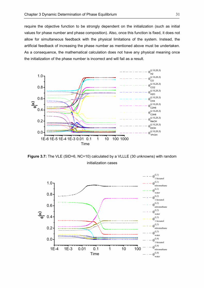
Chapter 3 Dynamic Determination of Phase Equilibrium 31
require the objective function to be strongly dependent on the initialization (such as initial
values for phase number and phase composition). Also, once this function is fixed, it does not
allow for simultaneous feedback with the physical limitations of the system. Instead, the
artificial feedback of increasing the phase number as mentioned above must be undertaken.
As a consequence, the mathematical calculation does not have any physical meaning once
the initialization of the phase number is incorrect and will fail as a result.
Figure 3.7: The VLE (SID=6, NC=10) calculated by a VLLLE (30 unknowns) with random
initialization cases
1E-6 1E-5 1E-4 1E-3 0.01 0.1 1 10 100 1000
0.0
0.2
0.4
0.6
0.8
1.0 θ
(L1/L2/L3)
H2
θ(L1/L2/L3)
CO
θ(L1/L2/L3)
CO2
θ(L1/L2/L3)
H2O
θ(L1/L2/L3)
CH4
θ(L1/L2/L3)
C2H6
θ(L1/L2/L3)
C3H8
θ(L1/L2/L3)
MeOH
θ(L1/L2/L3)
EtOH
θ(L1/L2/L3)
1PrOH
Time
θθ θθ( αα αα)
i
1E-4 1E-3 0.01 0.1 1 10 100
0.0
0.2
0.4
0.6
0.8
1.0
θ(L1)
1-hexanol
θ(L1)
nitromethane
θ(L1)
water
θ(L2)
1-hexanol
θ(L2)
nitromethane
θ(L2)
water
θ(L3)
1-hexanol
θ(L3)
nitromethane
θ(L3)
water
θ(L4)
1-hexanol
θ(L4)
nitromethane
θ(L4)
water
θθ θθ( αα αα)
i
Time
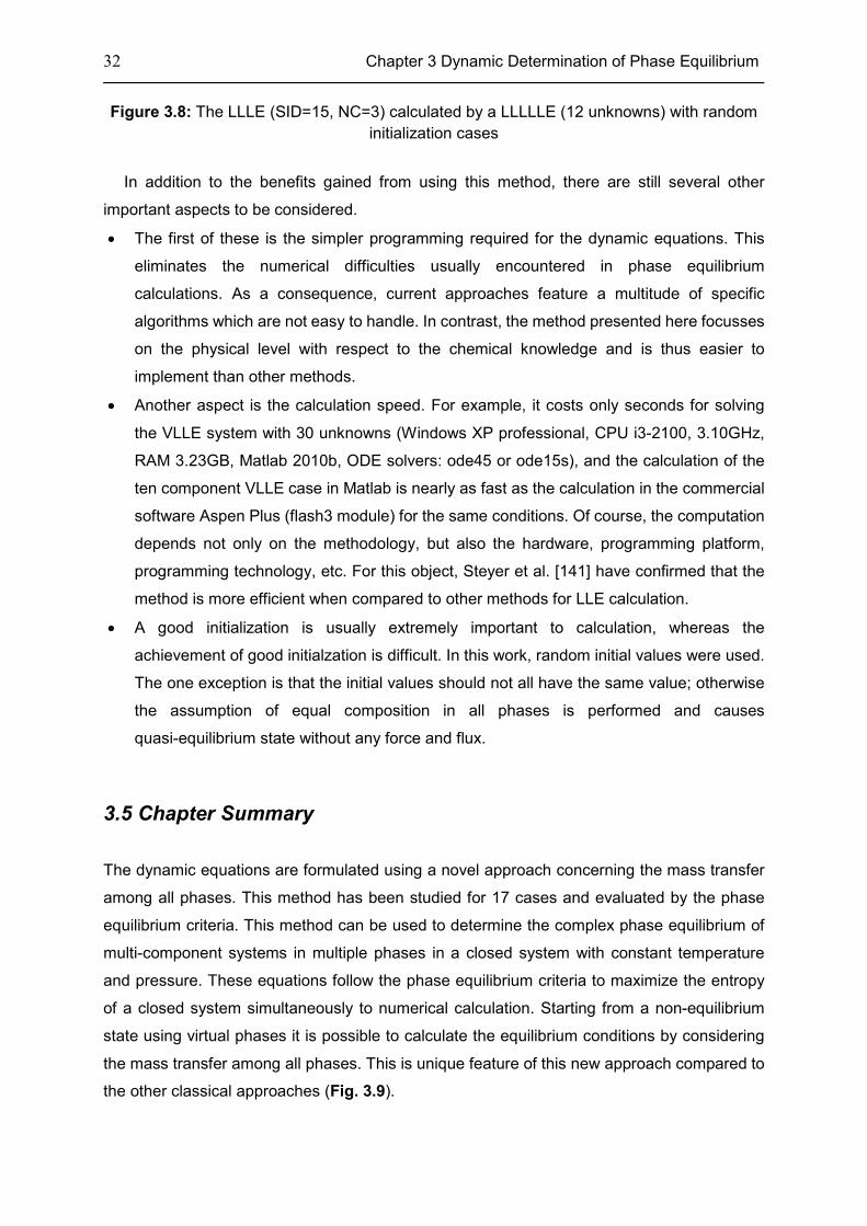
32 Chapter 3 Dynamic Determination of Phase Equilibrium
Figure 3.8: The LLLE (SID=15, NC=3) calculated by a LLLLLE (12 unknowns) with random
initialization cases
In addition to the benefits gained from using this method, there are still several other
important aspects to be considered.
• The first of these is the simpler programming required for the dynamic equations. This
eliminates the numerical difficulties usually encountered in phase equilibrium
calculations. As a consequence, current approaches feature a multitude of specific
algorithms which are not easy to handle. In contrast, the method presented here focusses
on the physical level with respect to the chemical knowledge and is thus easier to
implement than other methods.
• Another aspect is the calculation speed. For example, it costs only seconds for solving
the VLLE system with 30 unknowns (Windows XP professional, CPU i3-2100, 3.10GHz,
RAM 3.23GB, Matlab 2010b, ODE solvers: ode45 or ode15s), and the calculation of the
ten component VLLE case in Matlab is nearly as fast as the calculation in the commercial
software Aspen Plus (flash3 module) for the same conditions. Of course, the computation
depends not only on the methodology, but also the hardware, programming platform,
programming technology, etc. For this object, Steyer et al. [141] have confirmed that the
method is more efficient when compared to other methods for LLE calculation.
• A good initialization is usually extremely important to calculation, whereas the
achievement of good initialzation is difficult. In this work, random initial values were used.
The one exception is that the initial values should not all have the same value; otherwise
the assumption of equal composition in all phases is performed and causes
quasi-equilibrium state without any force and flux.
3.5 Chapter Summary
The dynamic equations are formulated using a novel approach concerning the mass transfer
among all phases. This method has been studied for 17 cases and evaluated by the phase
equilibrium criteria. This method can be used to determine the complex phase equilibrium of
multi-component systems in multiple phases in a closed system with constant temperature
and pressure. These equations follow the phase equilibrium criteria to maximize the entropy
of a closed system simultaneously to numerical calculation. Starting from a non-equilibrium
state using virtual phases it is possible to calculate the equilibrium conditions by considering
the mass transfer among all phases. This is unique feature of this new approach compared to
the other classical approaches (Fig. 3.9).
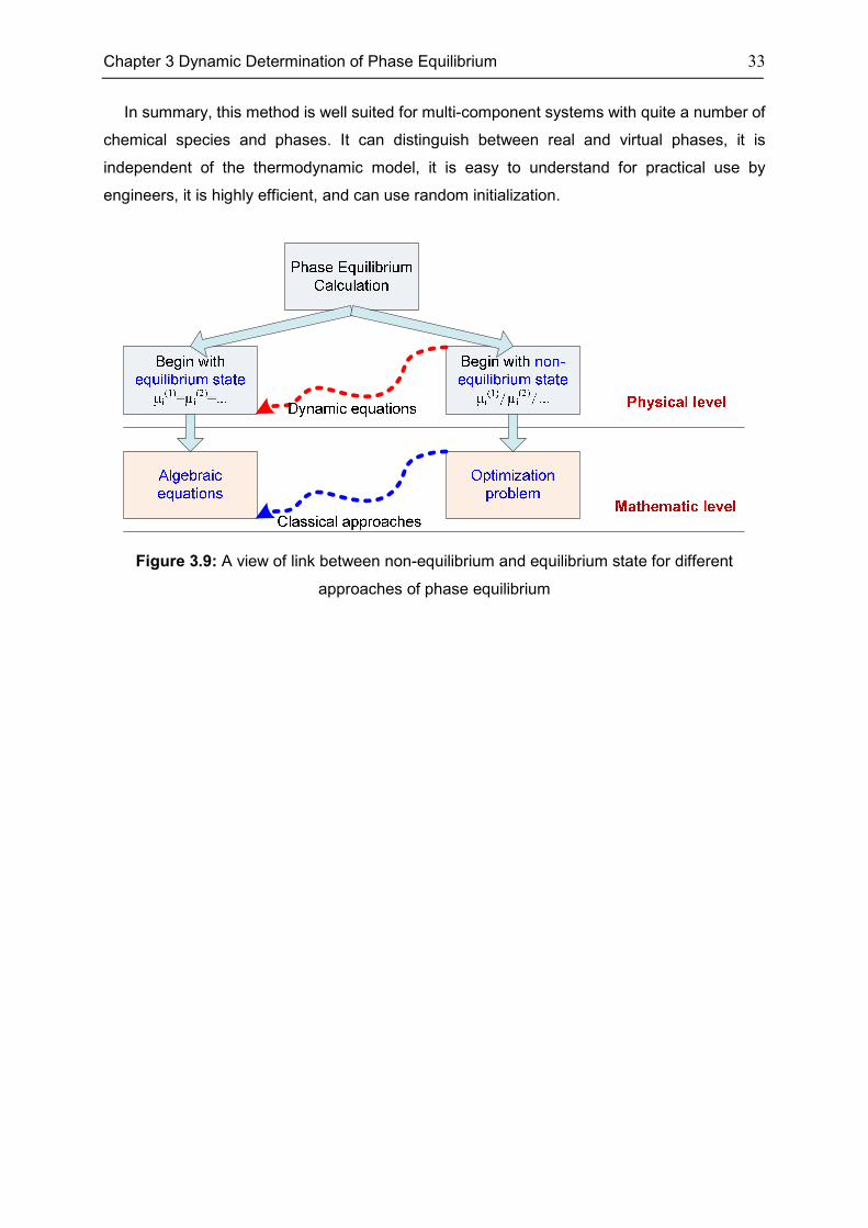
Chapter 3 Dynamic Determination of Phase Equilibrium 33
In summary, this method is well suited for multi-component systems with quite a number of
chemical species and phases. It can distinguish between real and virtual phases, it is
independent of the thermodynamic model, it is easy to understand for practical use by
engineers, it is highly efficient, and can use random initialization.
Figure 3.9: A view of link between non-equilibrium and equilibrium state for different
approaches of phase equilibrium
Part II
Applications
Chapter 4
Azeotropic Mixture Separation Using CO2
The last two chapters in Part I focus on the identification of phase behavior, in particular with
CXLs. With this basis, the application of CXLs in separation processes and reaction
processes will be illustrated in the coming two chapters (Part II), respectively. The effect of
phase behavior variation in the phase level on the higher hierarchical levels will be
investigated comprehensively.
In this chapter, a particular separation concept for the azeotropic mixture separation by
phase behavior tuning using pressurized CO2 is proposed, and then corresponding process
variants are founded and validated in the process simulation. The significant potential of the
new process is indicative of an economic alternative to separate azeotropic mixtures using
this concept.
4.1 Introduction
The most popular application of CO2 is the supercritical extraction [143]. The principle is that
substances are able to be dissolved in scCO2 dramatically. In another word, CO2 plays a role
of ‘extractor’ as scCO2. There is another concept of separation using CO2, and the principle is
that CO2 can change miscibility. An interesting experimental phenomenon has been
discovered in the 1950s [144, 145]. It is illustrated as follows. Homogeneous aqueous
solutions of alcohols or other polar solvents can be split into two liquid phases by pressurized
gases, so called ‘salting out’ agents [35, 145]. In this regard, CO2 is one of the most popular
‘salting out’ agents. The liquid can be split into two liquids as a VLLE phase behavior by
pressurizing CO2, and the transition occurs at the lower critical solution pressure (LCSP). The
liquid splits into an organic-rich liquid phase and a water-rich liquid phase. If the pressure is
The separation of chemical mixtures into their
constituents has been practiced, as an art, for
millennia.
J. D. Seader, et al.
Separation Process Principles, 1998
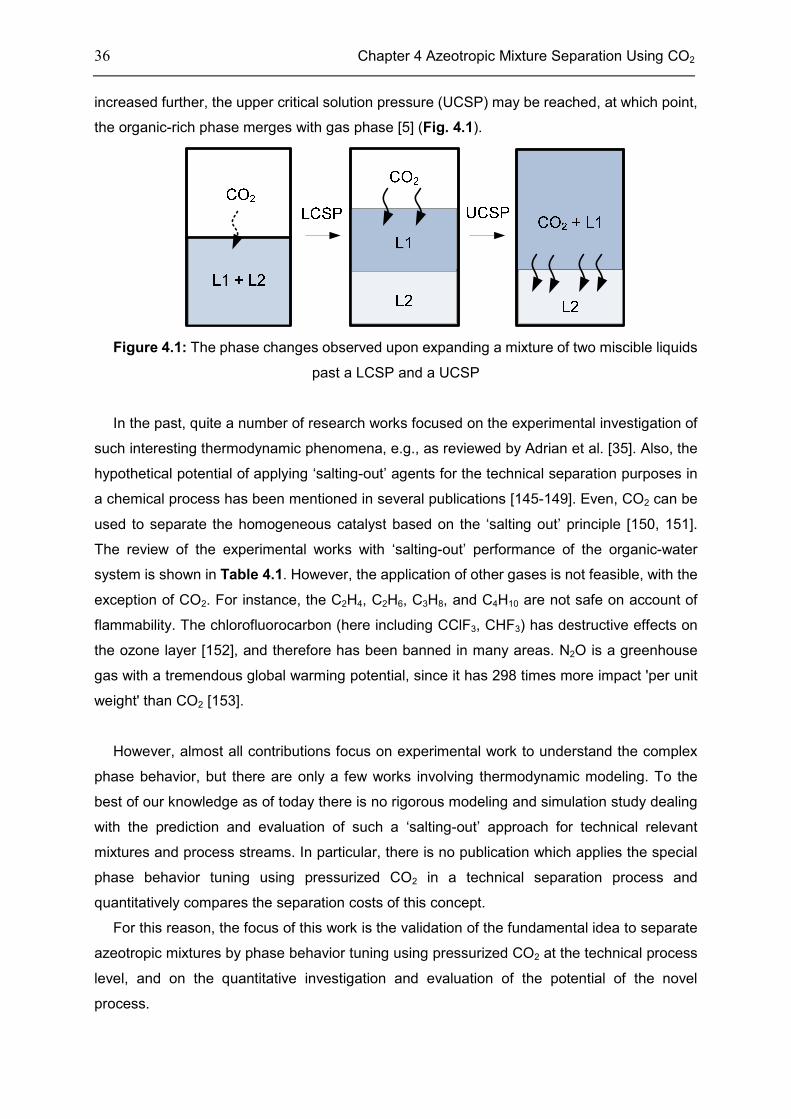
36 Chapter 4 Azeotropic Mixture Separation Using CO2
increased further, the upper critical solution pressure (UCSP) may be reached, at which point,
the organic-rich phase merges with gas phase [5] (Fig. 4.1).
Figure 4.1: The phase changes observed upon expanding a mixture of two miscible liquids
past a LCSP and a UCSP
In the past, quite a number of research works focused on the experimental investigation of
such interesting thermodynamic phenomena, e.g., as reviewed by Adrian et al. [35]. Also, the
hypothetical potential of applying ‘salting-out’ agents for the technical separation purposes in
a chemical process has been mentioned in several publications [145-149]. Even, CO2 can be
used to separate the homogeneous catalyst based on the ‘salting out’ principle [150, 151].
The review of the experimental works with ‘salting-out’ performance of the organic-water
system is shown in Table 4.1. However, the application of other gases is not feasible, with the
exception of CO2. For instance, the C2H4, C2H6, C3H8, and C4H10 are not safe on account of
flammability. The chlorofluorocarbon (here including CClF3, CHF3) has destructive effects on
the ozone layer [152], and therefore has been banned in many areas. N2O is a greenhouse
gas with a tremendous global warming potential, since it has 298 times more impact 'per unit
weight' than CO2 [153].
However, almost all contributions focus on experimental work to understand the complex
phase behavior, but there are only a few works involving thermodynamic modeling. To the
best of our knowledge as of today there is no rigorous modeling and simulation study dealing
with the prediction and evaluation of such a ‘salting-out’ approach for technical relevant
mixtures and process streams. In particular, there is no publication which applies the special
phase behavior tuning using pressurized CO2 in a technical separation process and
quantitatively compares the separation costs of this concept.
For this reason, the focus of this work is the validation of the fundamental idea to separate
azeotropic mixtures by phase behavior tuning using pressurized CO2 at the technical process
level, and on the quantitative investigation and evaluation of the potential of the novel
process.
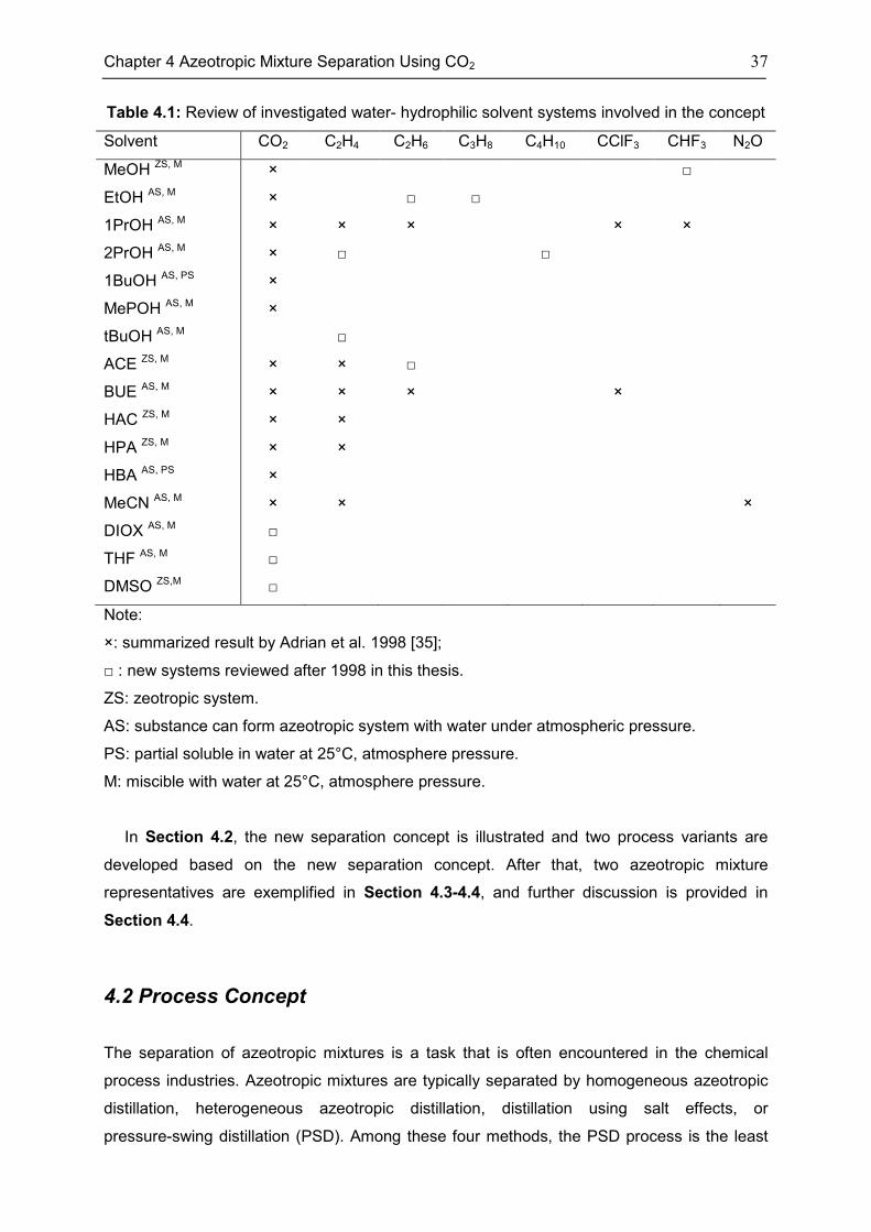
Chapter 4 Azeotropic Mixture Separation Using CO2 37
Table 4.1: Review of investigated water- hydrophilic solvent systems involved in the concept
Solvent CO2 C2H4 C2H6 C3H8 C4H10 CClF3 CHF3 N2O
MeOH ZS, M × □
EtOH AS, M × □ □
1PrOH AS, M × × × × ×
2PrOH AS, M × □ □
1BuOH AS, PS ×
MePOH AS, M ×
tBuOH AS, M □
ACE ZS, M × × □
BUE AS, M × × × ×
HAC ZS, M × ×
HPA ZS, M × ×
HBA AS, PS ×
MeCN AS, M × × ×
DIOX AS, M □
THF AS, M □
DMSO ZS,M □
Note:
×: summarized result by Adrian et al. 1998 [35];
□ : new systems reviewed after 1998 in this thesis.
ZS: zeotropic system.
AS: substance can form azeotropic system with water under atmospheric pressure.
PS: partial soluble in water at 25°C, atmosphere pressure.
M: miscible with water at 25°C, atmosphere pressure.
In Section 4.2, the new separation concept is illustrated and two process variants are
developed based on the new separation concept. After that, two azeotropic mixture
representatives are exemplified in Section 4.3-4.4, and further discussion is provided in
Section 4.4.
4.2 Process Concept
The separation of azeotropic mixtures is a task that is often encountered in the chemical
process industries. Azeotropic mixtures are typically separated by homogeneous azeotropic
distillation, heterogeneous azeotropic distillation, distillation using salt effects, or
pressure-swing distillation (PSD). Among these four methods, the PSD process is the least
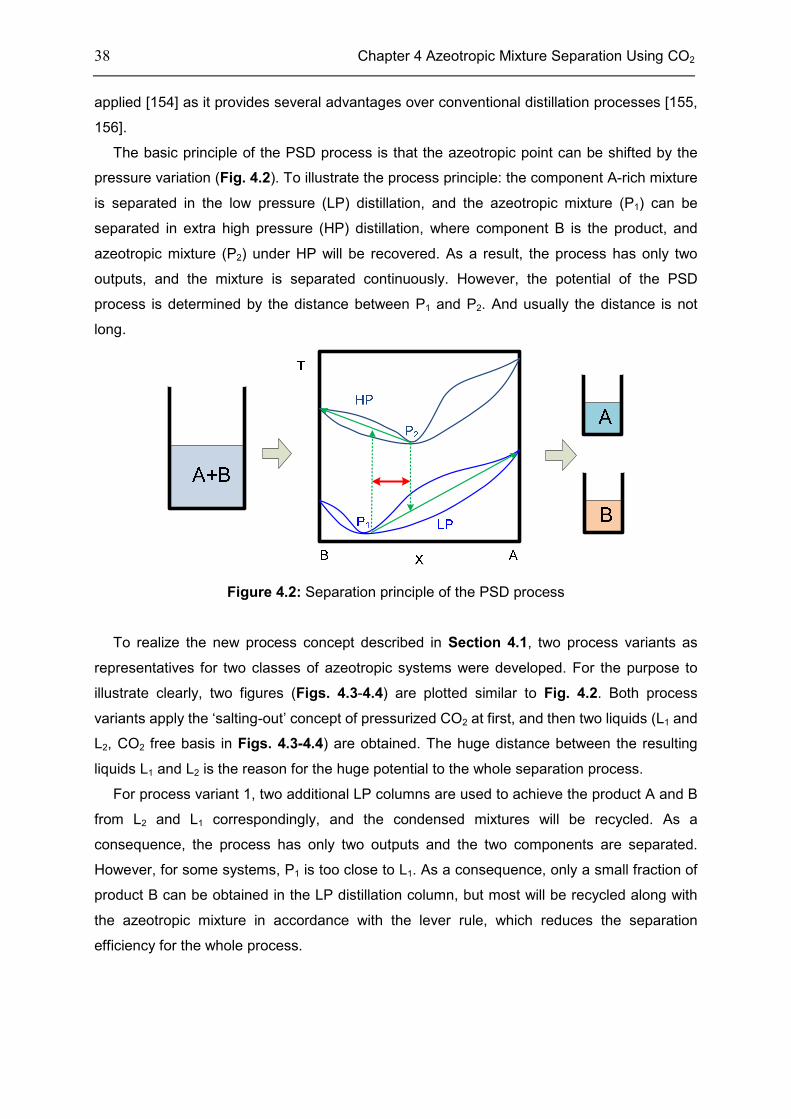
38 Chapter 4 Azeotropic Mixture Separation Using CO2
applied [154] as it provides several advantages over conventional distillation processes [155,
156].
The basic principle of the PSD process is that the azeotropic point can be shifted by the
pressure variation (Fig. 4.2). To illustrate the process principle: the component A-rich mixture
is separated in the low pressure (LP) distillation, and the azeotropic mixture (P1) can be
separated in extra high pressure (HP) distillation, where component B is the product, and
azeotropic mixture (P2) under HP will be recovered. As a result, the process has only two
outputs, and the mixture is separated continuously. However, the potential of the PSD
process is determined by the distance between P1 and P2. And usually the distance is not
long.
Figure 4.2: Separation principle of the PSD process
To realize the new process concept described in Section 4.1, two process variants as
representatives for two classes of azeotropic systems were developed. For the purpose to
illustrate clearly, two figures (Figs. 4.3-4.4) are plotted similar to Fig. 4.2. Both process
variants apply the ‘salting-out’ concept of pressurized CO2 at first, and then two liquids (L1 and
L2, CO2 free basis in Figs. 4.3-4.4) are obtained. The huge distance between the resulting
liquids L1 and L2 is the reason for the huge potential to the whole separation process.
For process variant 1, two additional LP columns are used to achieve the product A and B
from L2 and L1 correspondingly, and the condensed mixtures will be recycled. As a
consequence, the process has only two outputs and the two components are separated.
However, for some systems, P1 is too close to L1. As a consequence, only a small fraction of
product B can be obtained in the LP distillation column, but most will be recycled along with
the azeotropic mixture in accordance with the lever rule, which reduces the separation
efficiency for the whole process.
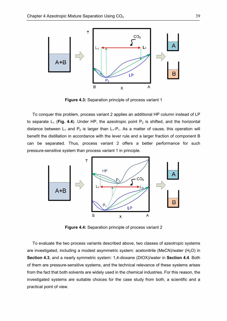
Chapter 4 Azeotropic Mixture Separation Using CO2 39
Figure 4.3: Separation principle of process variant 1
To conquer this problem, process variant 2 applies an additional HP column instead of LP
to separate L1 (Fig. 4.4). Under HP, the azeotropic point P2 is shifted, and the horizontal
distance between L1 and P2 is larger than L1-P1. As a matter of cause, this operation will
benefit the distillation in accordance with the lever rule and a larger fraction of component B
can be separated. Thus, process variant 2 offers a better performance for such
pressure-sensitive system than process variant 1 in principle.
Figure 4.4: Separation principle of process variant 2
To evaluate the two process variants described above, two classes of azeotropic systems
are investigated, including a modest asymmetric system: acetonitrile (MeCN)/water (H2O) in
Section 4.3, and a nearly symmetric system: 1,4-dioxane (DIOX)/water in Section 4.4. Both
of them are pressure-sensitive systems, and the technical relevance of these systems arises
from the fact that both solvents are widely used in the chemical industries. For this reason, the
investigated systems are suitable choices for the case study from both, a scientific and a
practical point of view.

40 Chapter 4 Azeotropic Mixture Separation Using CO2
A rigorous thermodynamic modeling is the base of a reliable process simulation. At the
beginning, the involved systems are modeled, which is described as follows: The VLE binary
systems (MeCN/H2O, DIOX/H2O) are predicted by NRTL-IG model (parameters are listed in
Table A2.6, the VLE diagrams are presented in Figs. A5.1-A5.4). In this approach, the NRTL
model is used for the description of the liquid phase behavior, and the vapor phase is
assumed as the ideal gas. The modeling steps and the performance of the model are
highlighted. The specific CEoS/GE model: PRWS is used for predicting the VLLE phase
behavior of the ternary systems (MeCN/H2O/CO2, DIOX/H2O/CO2). In this approach, all
phases are described by PRWS. The performance of the thermodynamic modeling is shown
in Section 2.3.
The proposed process variants and a conventional PSD process are simulated using the
commercial process simulation software Aspen Plus (V7.1). The VLLE phase behaviors are
predicted for a constant temperature (40°C) and modest pressures (pressure range
25bar-65bar for MeCN/H2O/CO2 system, 30bar-50bar for DIOX/H2O/CO2 system). The
rigorous equilibrium stage model is used for simulating the distillation. Nine different feed
compositions (xH2O=0.1-0.9 mol/mol, increasing increment 0.1) are investigated to evaluate
the potential composition range for the application of the new process variants. The feed flow
is always set to 100kmol/h; and the product quality is specified to xMeCN or DIOX=99.5% (mol/mol)
and xH2O=99.9% (mol/mol) for all cases.
Figure 4.5: Schematic of a conventional PSD process
The flowsheet of the conventional PSD process is shown in Fig. 4.5 and its specifications
of two systems are listed in Table 4.2. The feed is dependent on the azeotropic point location
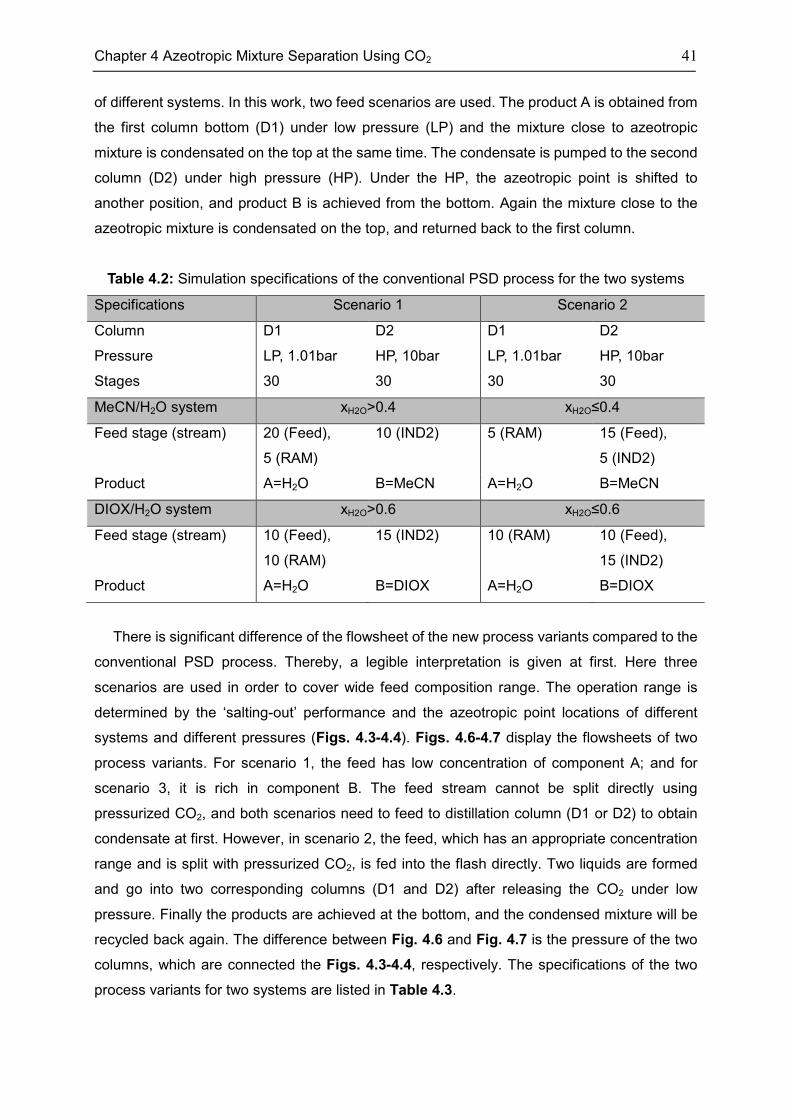
Chapter 4 Azeotropic Mixture Separation Using CO2 41
of different systems. In this work, two feed scenarios are used. The product A is obtained from
the first column bottom (D1) under low pressure (LP) and the mixture close to azeotropic
mixture is condensated on the top at the same time. The condensate is pumped to the second
column (D2) under high pressure (HP). Under the HP, the azeotropic point is shifted to
another position, and product B is achieved from the bottom. Again the mixture close to the
azeotropic mixture is condensated on the top, and returned back to the first column.
Table 4.2: Simulation specifications of the conventional PSD process for the two systems
Specifications Scenario 1 Scenario 2
Column D1 D2 D1 D2
Pressure LP, 1.01bar HP, 10bar LP, 1.01bar HP, 10bar
Stages 30 30 30 30
MeCN/H2O system xH2O>0.4 xH2O≤0.4
Feed stage (stream) 20 (Feed),
5 (RAM)
10 (IND2) 5 (RAM) 15 (Feed),
5 (IND2)
Product A=H2O B=MeCN A=H2O B=MeCN
DIOX/H2O system xH2O>0.6 xH2O≤0.6
Feed stage (stream) 10 (Feed),
10 (RAM)
15 (IND2) 10 (RAM) 10 (Feed),
15 (IND2)
Product A=H2O B=DIOX A=H2O B=DIOX
There is significant difference of the flowsheet of the new process variants compared to the
conventional PSD process. Thereby, a legible interpretation is given at first. Here three
scenarios are used in order to cover wide feed composition range. The operation range is
determined by the ‘salting-out’ performance and the azeotropic point locations of different
systems and different pressures (Figs. 4.3-4.4). Figs. 4.6-4.7 display the flowsheets of two
process variants. For scenario 1, the feed has low concentration of component A; and for
scenario 3, it is rich in component B. The feed stream cannot be split directly using
pressurized CO2, and both scenarios need to feed to distillation column (D1 or D2) to obtain
condensate at first. However, in scenario 2, the feed, which has an appropriate concentration
range and is split with pressurized CO2, is fed into the flash directly. Two liquids are formed
and go into two corresponding columns (D1 and D2) after releasing the CO2 under low
pressure. Finally the products are achieved at the bottom, and the condensed mixture will be
recycled back again. The difference between Fig. 4.6 and Fig. 4.7 is the pressure of the two
columns, which are connected the Figs. 4.3-4.4, respectively. The specifications of the two
process variants for two systems are listed in Table 4.3.
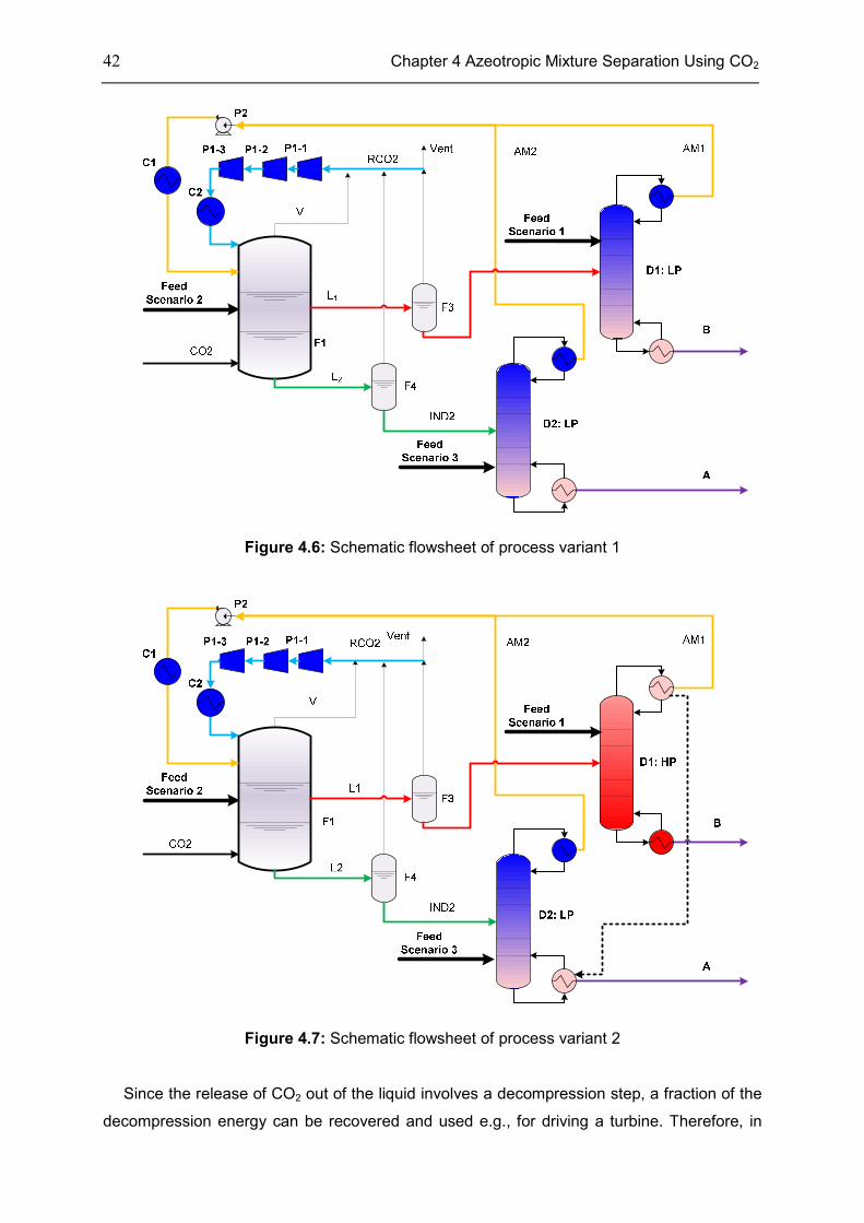
42 Chapter 4 Azeotropic Mixture Separation Using CO2
Figure 4.6: Schematic flowsheet of process variant 1
Figure 4.7: Schematic flowsheet of process variant 2
Since the release of CO2 out of the liquid involves a decompression step, a fraction of the
decompression energy can be recovered and used e.g., for driving a turbine. Therefore, in
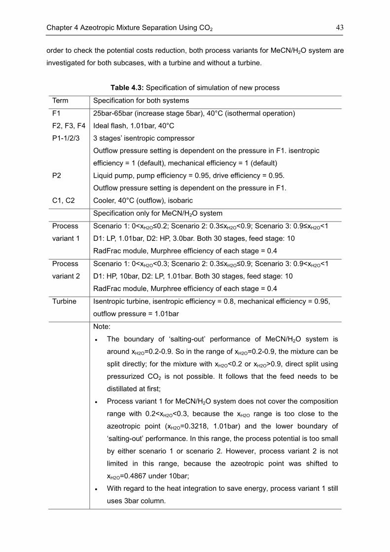
Chapter 4 Azeotropic Mixture Separation Using CO2 43
order to check the potential costs reduction, both process variants for MeCN/H2O system are
investigated for both subcases, with a turbine and without a turbine.
Table 4.3: Specification of simulation of new process
Term Specification for both systems
F1 25bar-65bar (increase stage 5bar), 40°C (isothermal operation)
F2, F3, F4 Ideal flash, 1.01bar, 40°C
P1-1/2/3 3 stages’ isentropic compressor
Outflow pressure setting is dependent on the pressure in F1. isentropic
efficiency = 1 (default), mechanical efficiency = 1 (default)
P2 Liquid pump, pump efficiency = 0.95, drive efficiency = 0.95.
Outflow pressure setting is dependent on the pressure in F1.
C1, C2 Cooler, 40°C (outflow), isobaric
Specification only for MeCN/H2O system
Process
variant 1
Scenario 1: 0<xH2O≤0.2; Scenario 2: 0.3≤xH2O<0.9; Scenario 3: 0.9≤xH2O<1
D1: LP, 1.01bar, D2: HP, 3.0bar. Both 30 stages, feed stage: 10
RadFrac module, Murphree efficiency of each stage = 0.4
Process
variant 2
Scenario 1: 0<xH2O<0.3; Scenario 2: 0.3≤xH2O≤0.9; Scenario 3: 0.9<xH2O<1
D1: HP, 10bar, D2: LP, 1.01bar. Both 30 stages, feed stage: 10
RadFrac module, Murphree efficiency of each stage = 0.4
Turbine Isentropic turbine, isentropic efficiency = 0.8, mechanical efficiency = 0.95,
outflow pressure = 1.01bar
Note:
• The boundary of ‘salting-out’ performance of MeCN/H2O system is
around xH2O=0.2-0.9. So in the range of xH2O=0.2-0.9, the mixture can be
split directly; for the mixture with xH2O<0.2 or xH2O>0.9, direct split using
pressurized CO2 is not possible. It follows that the feed needs to be
distillated at first;
• Process variant 1 for MeCN/H2O system does not cover the composition
range with 0.2<xH2O<0.3, because the xH2O range is too close to the
azeotropic point (xH2O=0.3218, 1.01bar) and the lower boundary of
‘salting-out’ performance. In this range, the process potential is too small
by either scenario 1 or scenario 2. However, process variant 2 is not
limited in this range, because the azeotropic point was shifted to
xH2O=0.4867 under 10bar;
• With regard to the heat integration to save energy, process variant 1 still
uses 3bar column.
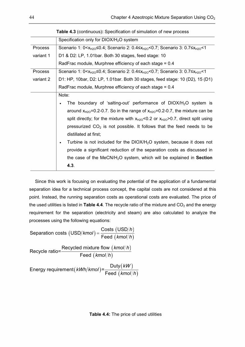
44 Chapter 4 Azeotropic Mixture Separation Using CO2
Table 4.3 (continuous): Specification of simulation of new process
Specification only for DIOX/H2O system
Process
variant 1
Scenario 1: 0<xH2O≤0.4; Scenario 2: 0.4≤xH2O<0.7; Scenario 3: 0.7≤xH2O<1
D1 & D2: LP, 1.01bar. Both 30 stages, feed stage: 10
RadFrac module, Murphree efficiency of each stage = 0.4
Process
variant 2
Scenario 1: 0<xH2O≤0.4; Scenario 2: 0.4≤xH2O<0.7; Scenario 3: 0.7≤xH2O<1
D1: HP, 10bar, D2: LP, 1.01bar. Both 30 stages, feed stage: 10 (D2), 15 (D1)
RadFrac module, Murphree efficiency of each stage = 0.4
Note:
• The boundary of ‘salting-out’ performance of DIOX/H2O system is
around xH2O=0.2-0.7. So in the range of xH2O=0.2-0.7, the mixture can be
split directly; for the mixture with xH2O<0.2 or xH2O>0.7, direct split using
pressurized CO2 is not possible. It follows that the feed needs to be
distillated at first;
• Turbine is not included for the DIOX/H2O system, because it does not
provide a significant reduction of the separation costs as discussed in
the case of the MeCN/H2O system, which will be explained in Section
4.3.
Since this work is focusing on evaluating the potential of the application of a fundamental
separation idea for a technical process concept, the capital costs are not considered at this
point. Instead, the running separation costs as operational costs are evaluated. The price of
the used utilities is listed in Table 4.4. The recycle ratio of the mixture and CO2 and the energy
requirement for the separation (electricity and steam) are also calculated to analyze the
processes using the following equations:
( ) ( )( )
=Costs USD
Separation costs USDFeed
hkmol
kmol h
( )( )
Recycled mixture flow Recycle ratio=
Feed
kmol h
kmol h
( ) ( )( )
DutyEnergy requirement =
Feed
kWkWh kmol
kmol h
Table 4.4: The price of used utilities
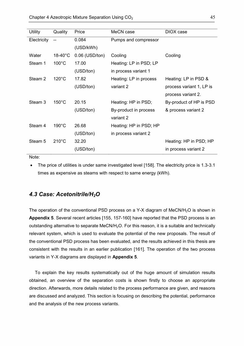
Chapter 4 Azeotropic Mixture Separation Using CO2 45
Utility Quality Price MeCN case DIOX case
Electricity -- 0.084
(USD/kWh)
Pumps and compressor
Water 18-40°C 0.06 (USD/ton) Cooling Cooling
Steam 1 100°C 17.00
(USD/ton)
Heating: LP in PSD; LP
in process variant 1
Steam 2 120°C 17.82
(USD/ton)
Heating: LP in process
variant 2
Heating: LP in PSD &
process variant 1, LP is
process variant 2.
Steam 3 150°C 20.15
(USD/ton)
Heating: HP in PSD;
By-product in process
variant 2
By-product of HP is PSD
& process variant 2
Steam 4 190°C 26.68
(USD/ton)
Heating: HP in PSD; HP
in process variant 2
Steam 5 210°C 32.20
(USD/ton)
Heating: HP in PSD; HP
in process variant 2
Note:
• The price of utilities is under same investigated level [158]. The electricity price is 1.3-3.1
times as expensive as steams with respect to same energy (kWh).
4.3 Case: Acetonitrile/H2O
The operation of the conventional PSD process on a Y-X diagram of MeCN/H2O is shown in
Appendix 5. Several recent articles [155, 157-160] have reported that the PSD process is an
outstanding alternative to separate MeCN/H2O. For this reason, it is a suitable and technically
relevant system, which is used to evaluate the potential of the new proposals. The result of
the conventional PSD process has been evaluated, and the results achieved in this thesis are
consistent with the results in an earlier publication [161]. The operation of the two process
variants in Y-X diagrams are displayed in Appendix 5.
To explain the key results systematically out of the huge amount of simulation results
obtained, an overview of the separation costs is shown firstly to choose an appropriate
direction. Afterwards, more details related to the process performance are given, and reasons
are discussed and analyzed. This section is focusing on describing the potential, performance
and the analysis of the new process variants.

46 Chapter 4 Azeotropic Mixture Separation Using CO2
Figure 4.8: Separation costs contrasting the
conventional PSD process and the two process
variants
Figure 4.9: Separation costs reduction of the two
process variants based on the conventional PSD
process
Note:
• Subcase 1: process variant 1 without turbine;
• Subcase 2: process variant 1 with turbine;
• Subcase 3: process variant 2 without turbine;
• Subcase 4: process variant 2 with turbine;
• PSD does not apply gas, and therefore no case with turbine is investigated.
Fig. 4.8 shows the overview of the separation costs contrasting the conventional PSD
process and the two process variants (case with the minimum separation costs among
investigated pressures). Two important results are summarized.
Firstly, the trend of the separation costs in the two process variants is similar, and both are
lower in comparison with the conventional PSD process for almost all cases. Thus, both of the
new process variants generally have potential to cut down the separation costs. Fig. 4.9
illustrates the separation costs reduction of the two process variants based on the
conventional PSD process. The process variant 1 offers a cost reduction of 23.8%~53.5% for
the feed composition range of 0.3≤xH2O≤0.9. With process variant 2 a cost reduction of
30.5%~68.9% is realized for a feed composition range of 0.1≤xH2O≤0.9. At lower water
fractions in the feed, however, process variant 1 features only little cost reduction potential (at
xH2O=0.2), and even higher costs are involved at xH2O=0.1. As a result, process variant 2 is
superior to process variant 1 regarding the separation costs.
As a second important result, the profiles of the separation costs with and without the
turbine are similar. Thus, the application of a turbine does not affect the energy costs
significantly; it only saves less than 5% for process variant 2 in general (Fig. 4.8).
0.0 0.2 0.4 0.6 0.8 1.00.0
0.3
0.6
0.9
1.2
1.5 conventional PSD
subcase 1
subcase 2
subcase 3
subcase 4
Separa
tion c
osts
(U
SD
/km
ol)
x(H2O)
0.0 0.2 0.4 0.6 0.8 1.0-80
-60
-40
-20
0
20
Se
para
tion c
osts
red
uction
(%
)
x(H2O)
subcase 1
subcase 2
subcase 3
subcase 4
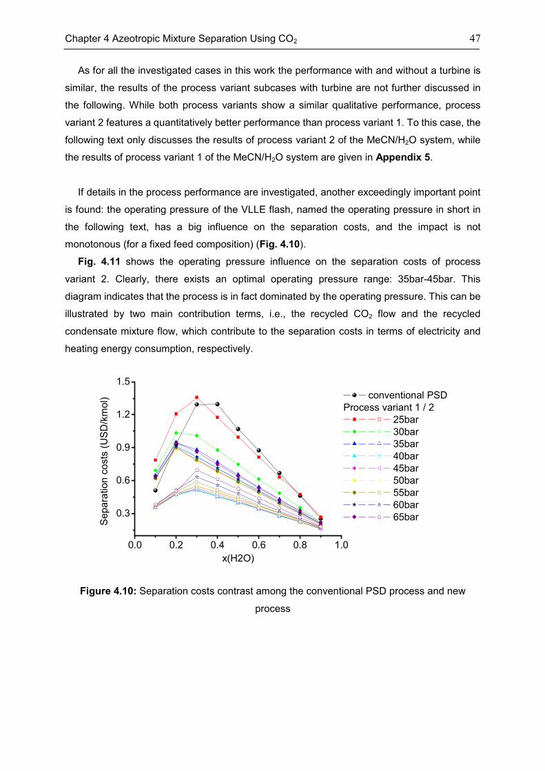
Chapter 4 Azeotropic Mixture Separation Using CO2 47
As for all the investigated cases in this work the performance with and without a turbine is
similar, the results of the process variant subcases with turbine are not further discussed in
the following. While both process variants show a similar qualitative performance, process
variant 2 features a quantitatively better performance than process variant 1. To this case, the
following text only discusses the results of process variant 2 of the MeCN/H2O system, while
the results of process variant 1 of the MeCN/H2O system are given in Appendix 5.
If details in the process performance are investigated, another exceedingly important point
is found: the operating pressure of the VLLE flash, named the operating pressure in short in
the following text, has a big influence on the separation costs, and the impact is not
monotonous (for a fixed feed composition) (Fig. 4.10).
Fig. 4.11 shows the operating pressure influence on the separation costs of process
variant 2. Clearly, there exists an optimal operating pressure range: 35bar-45bar. This
diagram indicates that the process is in fact dominated by the operating pressure. This can be
illustrated by two main contribution terms, i.e., the recycled CO2 flow and the recycled
condensate mixture flow, which contribute to the separation costs in terms of electricity and
heating energy consumption, respectively.
Figure 4.10: Separation costs contrast among the conventional PSD process and new
process
0.0 0.2 0.4 0.6 0.8 1.0
0.3
0.6
0.9
1.2
1.5
Separa
tion
co
sts
(U
SD
/km
ol)
x(H2O)
conventional PSD
Process variant 1 / 2
25bar
30bar
35bar
40bar
45bar
50bar
55bar
60bar
65bar
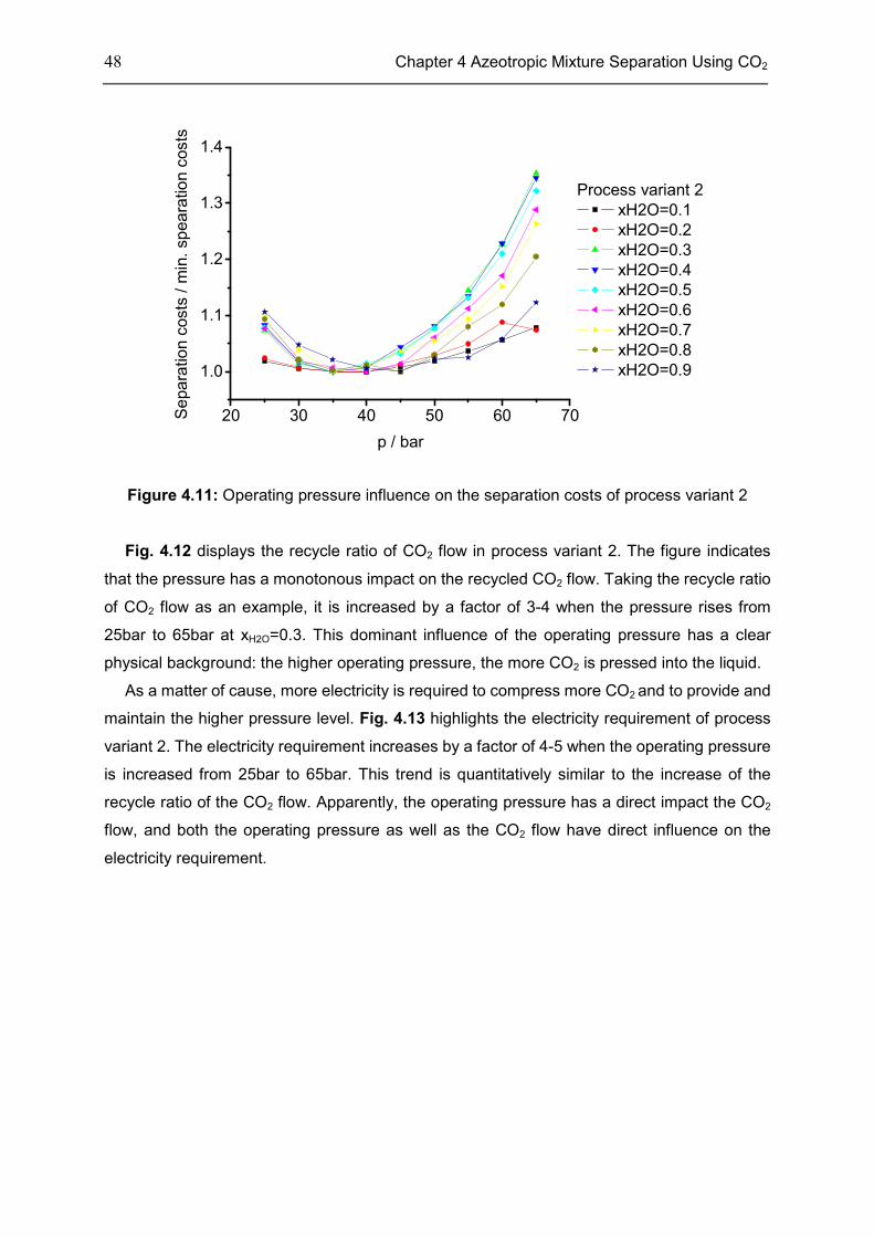
48 Chapter 4 Azeotropic Mixture Separation Using CO2
Figure 4.11: Operating pressure influence on the separation costs of process variant 2
Fig. 4.12 displays the recycle ratio of CO2 flow in process variant 2. The figure indicates
that the pressure has a monotonous impact on the recycled CO2 flow. Taking the recycle ratio
of CO2 flow as an example, it is increased by a factor of 3-4 when the pressure rises from
25bar to 65bar at xH2O=0.3. This dominant influence of the operating pressure has a clear
physical background: the higher operating pressure, the more CO2 is pressed into the liquid.
As a matter of cause, more electricity is required to compress more CO2 and to provide and
maintain the higher pressure level. Fig. 4.13 highlights the electricity requirement of process
variant 2. The electricity requirement increases by a factor of 4-5 when the operating pressure
is increased from 25bar to 65bar. This trend is quantitatively similar to the increase of the
recycle ratio of the CO2 flow. Apparently, the operating pressure has a direct impact the CO2
flow, and both the operating pressure as well as the CO2 flow have direct influence on the
electricity requirement.
20 30 40 50 60 70
1.0
1.1
1.2
1.3
1.4
Process variant 2
xH2O=0.1
xH2O=0.2
xH2O=0.3
xH2O=0.4
xH2O=0.5
xH2O=0.6
xH2O=0.7
xH2O=0.8
xH2O=0.9
Se
pa
ratio
n c
osts
/ m
in.
sp
ea
ratio
n c
osts
p / bar
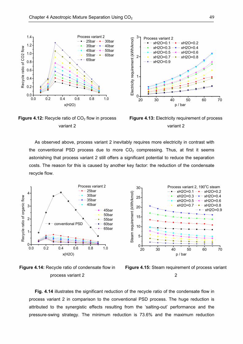
Chapter 4 Azeotropic Mixture Separation Using CO2 49
Figure 4.12: Recycle ratio of CO2 flow in process
variant 2
Figure 4.13: Electricity requirement of process
variant 2
As observed above, process variant 2 inevitably requires more electricity in contrast with
the conventional PSD process due to more CO2 compressing. Thus, at first it seems
astonishing that process variant 2 still offers a significant potential to reduce the separation
costs. The reason for this is caused by another key factor: the reduction of the condensate
recycle flow.
Figure 4.14: Recycle ratio of condensate flow in
process variant 2
Figure 4.15: Steam requirement of process variant
2
Fig. 4.14 illustrates the significant reduction of the recycle ratio of the condensate flow in
process variant 2 in comparison to the conventional PSD process. The huge reduction is
attributed to the synergistic effects resulting from the ‘salting-out’ performance and the
pressure-swing strategy. The minimum reduction is 73.6% and the maximum reduction
0.0 0.2 0.4 0.6 0.8 1.00.0
0.2
0.4
0.6
0.8
1.0
1.2
1.4 Process variant 2
25bar 30bar
35bar 40bar
45bar 50bar
55bar 60bar
65bar
Re
cycle
ra
tio
of
CO
2 f
low
x(H2O)
20 30 40 50 60 700
1
2
3 Process variant 2
xH2O=0.1 xH2O=0.2
xH2O=0.3 xH2O=0.4
xH2O=0.5 xH2O=0.6
xH2O=0.7 xH2O=0.8
xH2O=0.9
Ele
ctr
icity r
equ
irem
ent (k
Wh
/km
ol)
p / bar
0.0 0.2 0.4 0.6 0.8 1.00
1
2
3
4
45bar
50bar
55bar
60bar
65bar
Process variant 2
25bar
30bar
35bar
40bar
conventional PSD
Re
cycle
ra
tio
of
org
an
ic f
low
x(H2O)
20 30 40 50 60 700
5
10
15
20
25
30 Process variant 2, 190oC steam
xH2O=0.1 xH2O=0.2
xH2O=0.3 xH2O=0.4
xH2O=0.5 xH2O=0.6
xH2O=0.7 xH2O=0.8
xH2O=0.9
Ste
am
re
qu
ire
men
t (k
Wh
/km
ol)
p / bar
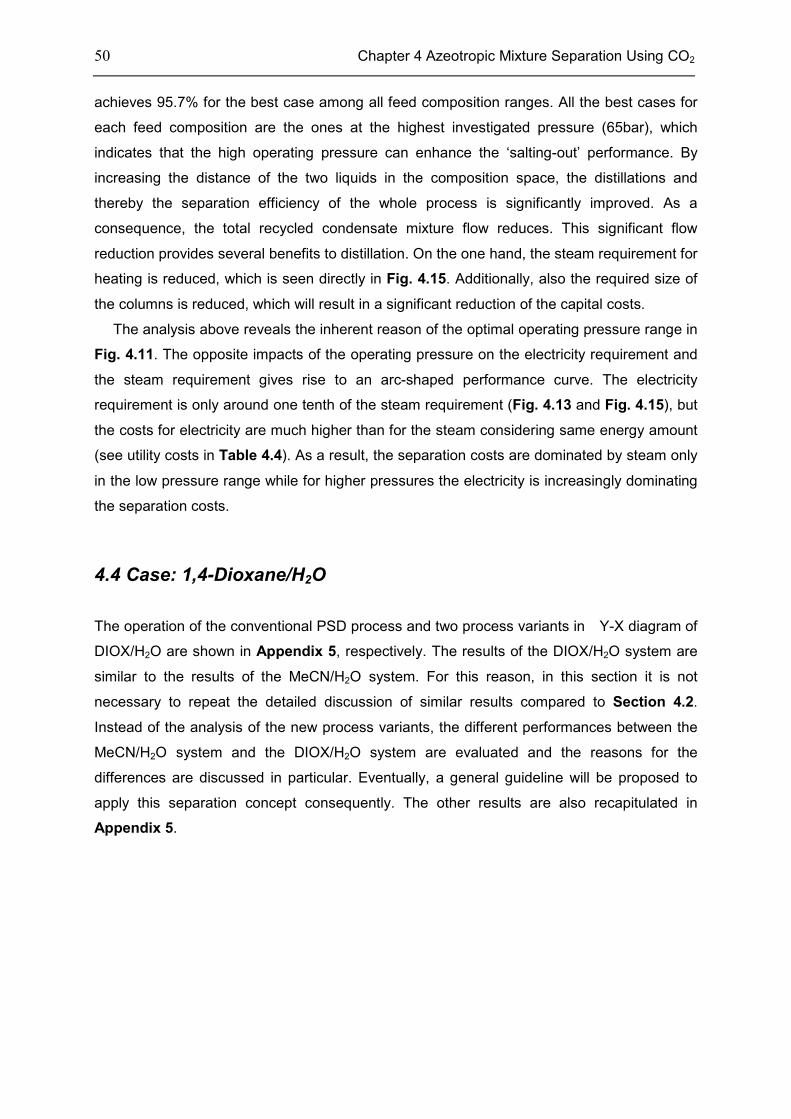
50 Chapter 4 Azeotropic Mixture Separation Using CO2
achieves 95.7% for the best case among all feed composition ranges. All the best cases for
each feed composition are the ones at the highest investigated pressure (65bar), which
indicates that the high operating pressure can enhance the ‘salting-out’ performance. By
increasing the distance of the two liquids in the composition space, the distillations and
thereby the separation efficiency of the whole process is significantly improved. As a
consequence, the total recycled condensate mixture flow reduces. This significant flow
reduction provides several benefits to distillation. On the one hand, the steam requirement for
heating is reduced, which is seen directly in Fig. 4.15. Additionally, also the required size of
the columns is reduced, which will result in a significant reduction of the capital costs.
The analysis above reveals the inherent reason of the optimal operating pressure range in
Fig. 4.11. The opposite impacts of the operating pressure on the electricity requirement and
the steam requirement gives rise to an arc-shaped performance curve. The electricity
requirement is only around one tenth of the steam requirement (Fig. 4.13 and Fig. 4.15), but
the costs for electricity are much higher than for the steam considering same energy amount
(see utility costs in Table 4.4). As a result, the separation costs are dominated by steam only
in the low pressure range while for higher pressures the electricity is increasingly dominating
the separation costs.
4.4 Case: 1,4-Dioxane/H2O
The operation of the conventional PSD process and two process variants in Y-X diagram of
DIOX/H2O are shown in Appendix 5, respectively. The results of the DIOX/H2O system are
similar to the results of the MeCN/H2O system. For this reason, in this section it is not
necessary to repeat the detailed discussion of similar results compared to Section 4.2.
Instead of the analysis of the new process variants, the different performances between the
MeCN/H2O system and the DIOX/H2O system are evaluated and the reasons for the
differences are discussed in particular. Eventually, a general guideline will be proposed to
apply this separation concept consequently. The other results are also recapitulated in
Appendix 5.
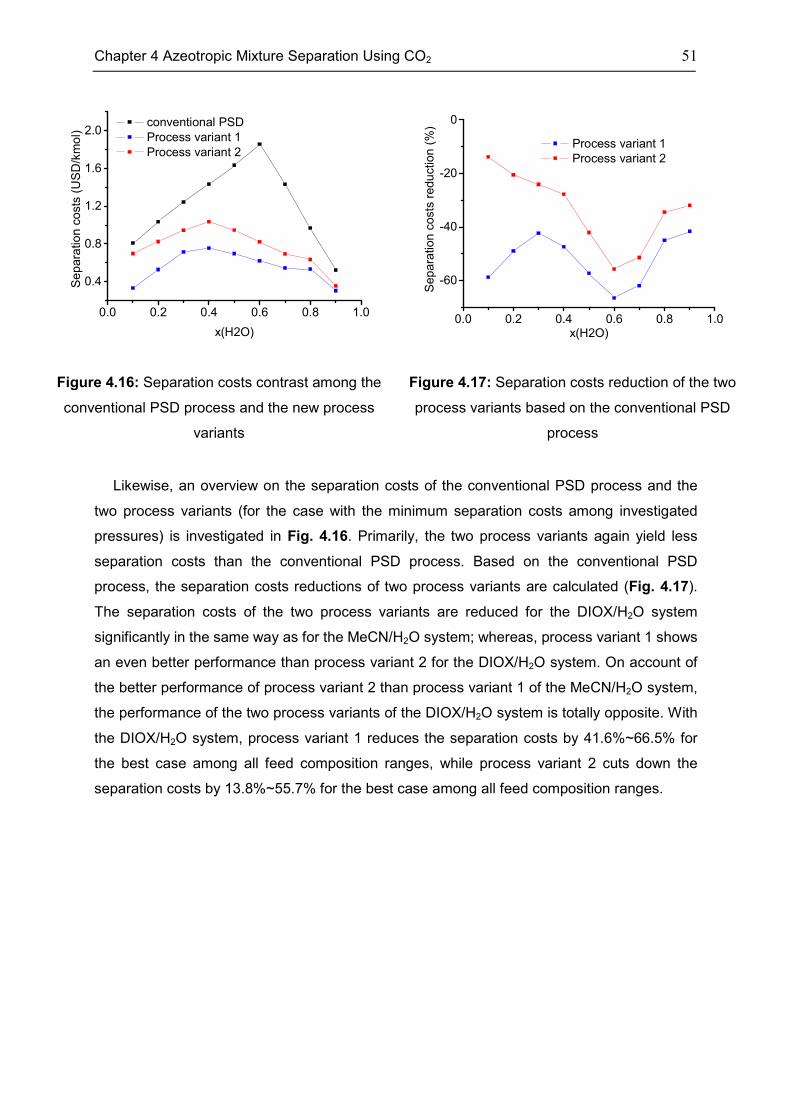
Chapter 4 Azeotropic Mixture Separation Using CO2 51
Figure 4.16: Separation costs contrast among the
conventional PSD process and the new process
variants
Figure 4.17: Separation costs reduction of the two
process variants based on the conventional PSD
process
Likewise, an overview on the separation costs of the conventional PSD process and the
two process variants (for the case with the minimum separation costs among investigated
pressures) is investigated in Fig. 4.16. Primarily, the two process variants again yield less
separation costs than the conventional PSD process. Based on the conventional PSD
process, the separation costs reductions of two process variants are calculated (Fig. 4.17).
The separation costs of the two process variants are reduced for the DIOX/H2O system
significantly in the same way as for the MeCN/H2O system; whereas, process variant 1 shows
an even better performance than process variant 2 for the DIOX/H2O system. On account of
the better performance of process variant 2 than process variant 1 of the MeCN/H2O system,
the performance of the two process variants of the DIOX/H2O system is totally opposite. With
the DIOX/H2O system, process variant 1 reduces the separation costs by 41.6%~66.5% for
the best case among all feed composition ranges, while process variant 2 cuts down the
separation costs by 13.8%~55.7% for the best case among all feed composition ranges.
0.0 0.2 0.4 0.6 0.8 1.0
0.4
0.8
1.2
1.6
2.0
Se
para
tio
n c
osts
(U
SD
/km
ol)
x(H2O)
conventional PSD
Process variant 1
Process variant 2
0.0 0.2 0.4 0.6 0.8 1.0
-60
-40
-20
0
Sep
ara
tion
costs
redu
ction (
%)
x(H2O)
Process variant 1
Process variant 2
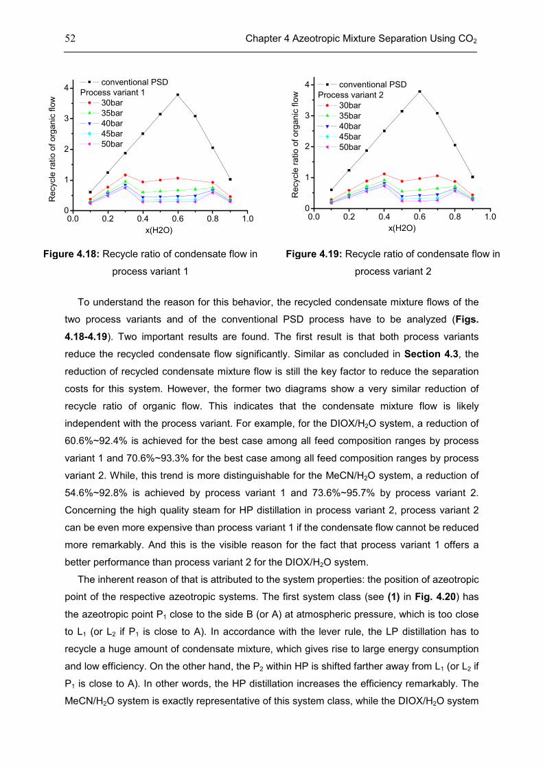
52 Chapter 4 Azeotropic Mixture Separation Using CO2
Figure 4.18: Recycle ratio of condensate flow in
process variant 1
Figure 4.19: Recycle ratio of condensate flow in
process variant 2
To understand the reason for this behavior, the recycled condensate mixture flows of the
two process variants and of the conventional PSD process have to be analyzed (Figs.
4.18-4.19). Two important results are found. The first result is that both process variants
reduce the recycled condensate flow significantly. Similar as concluded in Section 4.3, the
reduction of recycled condensate mixture flow is still the key factor to reduce the separation
costs for this system. However, the former two diagrams show a very similar reduction of
recycle ratio of organic flow. This indicates that the condensate mixture flow is likely
independent with the process variant. For example, for the DIOX/H2O system, a reduction of
60.6%~92.4% is achieved for the best case among all feed composition ranges by process
variant 1 and 70.6%~93.3% for the best case among all feed composition ranges by process
variant 2. While, this trend is more distinguishable for the MeCN/H2O system, a reduction of
54.6%~92.8% is achieved by process variant 1 and 73.6%~95.7% by process variant 2.
Concerning the high quality steam for HP distillation in process variant 2, process variant 2
can be even more expensive than process variant 1 if the condensate flow cannot be reduced
more remarkably. And this is the visible reason for the fact that process variant 1 offers a
better performance than process variant 2 for the DIOX/H2O system.
The inherent reason of that is attributed to the system properties: the position of azeotropic
point of the respective azeotropic systems. The first system class (see (1) in Fig. 4.20) has
the azeotropic point P1 close to the side B (or A) at atmospheric pressure, which is too close
to L1 (or L2 if P1 is close to A). In accordance with the lever rule, the LP distillation has to
recycle a huge amount of condensate mixture, which gives rise to large energy consumption
and low efficiency. On the other hand, the P2 within HP is shifted farther away from L1 (or L2 if
P1 is close to A). In other words, the HP distillation increases the efficiency remarkably. The
MeCN/H2O system is exactly representative of this system class, while the DIOX/H2O system
0.0 0.2 0.4 0.6 0.8 1.00
1
2
3
4
Re
cycle
ratio
of o
rga
nic
flo
w
x(H2O)
conventional PSD
Process variant 1
30bar
35bar
40bar
45bar
50bar
0.0 0.2 0.4 0.6 0.8 1.00
1
2
3
4
Recycle
ratio
of org
anic
flo
w
x(H2O)
conventional PSD
Process variant 2
30bar
35bar
40bar
45bar
50bar
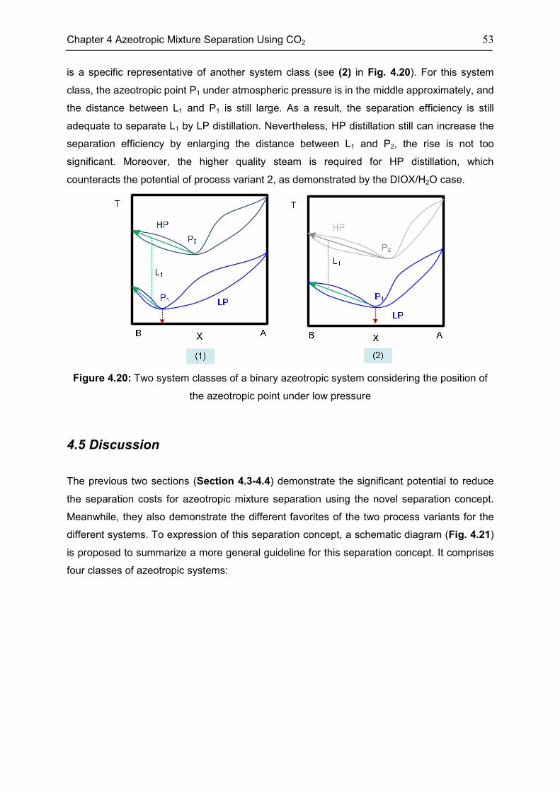
Chapter 4 Azeotropic Mixture Separation Using CO2 53
is a specific representative of another system class (see (2) in Fig. 4.20). For this system
class, the azeotropic point P1 under atmospheric pressure is in the middle approximately, and
the distance between L1 and P1 is still large. As a result, the separation efficiency is still
adequate to separate L1 by LP distillation. Nevertheless, HP distillation still can increase the
separation efficiency by enlarging the distance between L1 and P2, the rise is not too
significant. Moreover, the higher quality steam is required for HP distillation, which
counteracts the potential of process variant 2, as demonstrated by the DIOX/H2O case.
Figure 4.20: Two system classes of a binary azeotropic system considering the position of
the azeotropic point under low pressure
4.5 Discussion
The previous two sections (Section 4.3-4.4) demonstrate the significant potential to reduce
the separation costs for azeotropic mixture separation using the novel separation concept.
Meanwhile, they also demonstrate the different favorites of the two process variants for the
different systems. To expression of this separation concept, a schematic diagram (Fig. 4.21)
is proposed to summarize a more general guideline for this separation concept. It comprises
four classes of azeotropic systems:
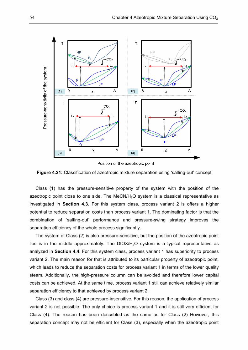
54 Chapter 4 Azeotropic Mixture Separation Using CO2
Figure 4.21: Classification of azeotropic mixture separation using ‘salting-out’ concept
Class (1) has the pressure-sensitive property of the system with the position of the
azeotropic point close to one side. The MeCN/H2O system is a classical representative as
investigated in Section 4.3. For this system class, process variant 2 is offers a higher
potential to reduce separation costs than process variant 1. The dominating factor is that the
combination of ‘salting-out’ performance and pressure-swing strategy improves the
separation efficiency of the whole process significantly.
The system of Class (2) is also pressure-sensitive, but the position of the azeotropic point
lies is in the middle approximately. The DIOX/H2O system is a typical representative as
analyzed in Section 4.4. For this system class, process variant 1 has superiority to process
variant 2. The main reason for that is attributed to its particular property of azeotropic point,
which leads to reduce the separation costs for process variant 1 in terms of the lower quality
steam. Additionally, the high-pressure column can be avoided and therefore lower capital
costs can be achieved. At the same time, process variant 1 still can achieve relatively similar
separation efficiency to that achieved by process variant 2.
Class (3) and class (4) are pressure-insensitive. For this reason, the application of process
variant 2 is not possible. The only choice is process variant 1 and it is still very efficient for
Class (4). The reason has been describled as the same as for Class (2) However, this
separation concept may not be efficient for Class (3), especially when the azeotropic point
Chapter 4 Azeotropic Mixture Separation Using CO2 55
(P1) is too close to L1. The smaller the distance between P1 and L1, the lower the separation
efficiency of the whole system. Moreover, once the azeotropic point (P1) does not lie between
L1 and L2, this separation concept cannot be used any longer for such extremely azeotropic
systems. A possible system could be e.g., the water and ethanol system, since the azeotropic
point is highly rich in ethanol (~90% ethanol (mol/mol)).
It should be noted that the feed composition considered in this thesis varies in a broad
range, which yields also a large variation with regard to the size of equipment. In this
fundamental study, it is not yet the aim to estimate capital costs quantitatively. However, a
qualitative analysis can be still performed at this point. The new process variants require a
higher number of equipment components compared to the conventional PSD process (i.e.,
flash tanks, coolers, and compressors), however, the significant reduction of recycled
condensate mixture flow (e.g., 73.6%~95.7% reduction for the best case among all feed
composition ranges by process variant 2 for MeCN/H2O system) decreases the distillation
column size drastically. As a consequence, the capital costs of the new process can
potentially be even lower than the capital costs of the conventional PSD process, because the
distillation columns are usually a main factor being much more expensive than other
equipment components.
4.6 Chapter Summary
This chapter demonstrates a conceptual idea to transfer the phase tuning information from the
phase level to the higher hierarchical process levels. In detail, pressurized CO2 is used to
change the miscibility of homogeneous mixtures on the phase level, while on higher levels, a
technical approach for azeotropic mixture separation based on the phase behavior tuning is
performed.
For validating the separation concept, two process variants are proposed and developed.
After that, the performance of the new process variants is evaluated. Two azeotropic systems,
i.e., the MeCN/H2O system and the DIOX/H2O system, which are representatives for Class (1)
and Class (2), in particular, are investigated in case studies by means of process simulation.
The results are compared to that of the technical reference process scheme, i.e., a
conventional PSD separation process. A significant reduction of the separation costs when
compared to the conventional PSD process for both systems can be achieved, although the
new process variants consume more electricity than the conventional PSD process. The main
reason for the achievement of the significant reduction as analyzed is that the significant
increase of separation efficiency through the phase behavior tuning leads to a remarkable
reduction of the recycled condensate mixture. Thus, these results clearly turn out that the
novel fundamental separation approach by phase behavior tuning using pressurized CO2 is a
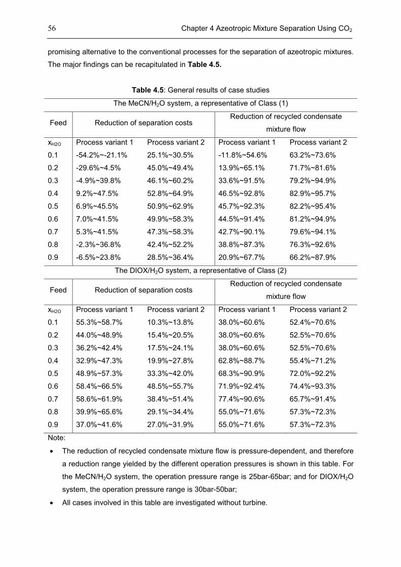
56 Chapter 4 Azeotropic Mixture Separation Using CO2
promising alternative to the conventional processes for the separation of azeotropic mixtures.
The major findings can be recapitulated in Table 4.5.
Table 4.5: General results of case studies
The MeCN/H2O system, a representative of Class (1)
Feed Reduction of separation costs Reduction of recycled condensate
mixture flow
xH2O Process variant 1 Process variant 2 Process variant 1 Process variant 2
0.1 -54.2%~-21.1% 25.1%~30.5% -11.8%~54.6% 63.2%~73.6%
0.2 -29.6%~4.5% 45.0%~49.4% 13.9%~65.1% 71.7%~81.6%
0.3 -4.9%~39.8% 46.1%~60.2% 33.6%~91.5% 79.2%~94.9%
0.4 9.2%~47.5% 52.8%~64.9% 46.5%~92.8% 82.9%~95.7%
0.5 6.9%~45.5% 50.9%~62.9% 45.7%~92.3% 82.2%~95.4%
0.6 7.0%~41.5% 49.9%~58.3% 44.5%~91.4% 81.2%~94.9%
0.7 5.3%~41.5% 47.3%~58.3% 42.7%~90.1% 79.6%~94.1%
0.8 -2.3%~36.8% 42.4%~52.2% 38.8%~87.3% 76.3%~92.6%
0.9 -6.5%~23.8% 28.5%~36.4% 20.9%~67.7% 66.2%~87.9%
The DIOX/H2O system, a representative of Class (2)
Feed Reduction of separation costs Reduction of recycled condensate
mixture flow
xH2O Process variant 1 Process variant 2 Process variant 1 Process variant 2
0.1 55.3%~58.7% 10.3%~13.8% 38.0%~60.6% 52.4%~70.6%
0.2 44.0%~48.9% 15.4%~20.5% 38.0%~60.6% 52.5%~70.6%
0.3 36.2%~42.4% 17.5%~24.1% 38.0%~60.6% 52.5%~70.6%
0.4 32.9%~47.3% 19.9%~27.8% 62.8%~88.7% 55.4%~71.2%
0.5 48.9%~57.3% 33.3%~42.0% 68.3%~90.9% 72.0%~92.2%
0.6 58.4%~66.5% 48.5%~55.7% 71.9%~92.4% 74.4%~93.3%
0.7 58.6%~61.9% 38.4%~51.4% 77.4%~90.6% 65.7%~91.4%
0.8 39.9%~65.6% 29.1%~34.4% 55.0%~71.6% 57.3%~72.3%
0.9 37.0%~41.6% 27.0%~31.9% 55.0%~71.6% 57.3%~72.3%
Note:
• The reduction of recycled condensate mixture flow is pressure-dependent, and therefore
a reduction range yielded by the different operation pressures is shown in this table. For
the MeCN/H2O system, the operation pressure range is 25bar-65bar; and for DIOX/H2O
system, the operation pressure range is 30bar-50bar;
• All cases involved in this table are investigated without turbine.

Chapter 4 Azeotropic Mixture Separation Using CO2 57
Besides, the selection of a suitable process variant is dominated by the properties of the
pressure-sensitivity and the position of the azeotropic point. The potential of using the new
separation concept is generalized and four classes of azeotropic systems are classified.
Concerning the negative environmental impact from quite a number of the traditional
organic solvents that are used in a wide application range and at large scale, the new
separation technology presented in this thesis using the benign solvent CO2 seems attractive
and may help to pave the way towards more sustainable separation processes.
Chapter 5
Reaction Intensification Using CO2
The previous chapter describes a new process for the separation of azeotropic mixtures by
phase behavior tuning using CO2, and this chapter will investigate reaction intensification
using CO2, following a brief review on reactions in CXLs (Section 5.1). Because of the active
research in the field of long-chain alkene hydroformylation, it is selected and reviewed briefly
as an example for further research.
Following this, in Section 5.2, the four factors of solvent type, solvent quantity,
temperature, and pressure, are investigated, and their influence on a 1-octene
hydroformylation system with respect to H2 solubility, CO solubility, the H2/CO ratio, and CO2
solubility is thermodynamically evaluated. In Section 5.3, a proposal to combine two solvent
concepts for long-chain alkene hydroformylation is also discussed.
5.1 Introduction
Recently, three reactions carried out in CXLs, i.e., oxidation, hydrogenation, and
hydroformylation, have received particular attention, since all of them involve several
permanent gases, H2, CO, and O2. One feature of CXLs is their ability to increase the
solubility of permanent gases. Furthermore, CXLs favor homogeneous as well as
heterogeneous reactions in terms of improving mass transfer and strengthening safety
through fire suppression. This is especially important for systems involving hydrogen and
oxygen. A brief review of these three reaction classes in CXLs is given in Table 5.1.
Reactor design uses information, knowledge, and
experience from a variety of areas -thermodynamics,
chemical kinetics, fluid mechanics, heat transfer, mass
transfer, and economics.
Octave Levenspiel
Chemical Reaction Engineering, 3rd ed.,1999
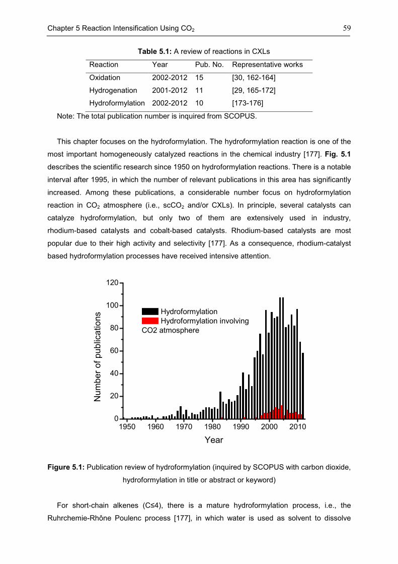
Chapter 5 Reaction Intensification Using CO2 59
Table 5.1: A review of reactions in CXLs
Reaction Year Pub. No. Representative works
Oxidation 2002-2012 15 [30, 162-164]
Hydrogenation 2001-2012 11 [29, 165-172]
Hydroformylation 2002-2012 10 [173-176]
Note: The total publication number is inquired from SCOPUS.
This chapter focuses on the hydroformylation. The hydroformylation reaction is one of the
most important homogeneously catalyzed reactions in the chemical industry [177]. Fig. 5.1
describes the scientific research since 1950 on hydroformylation reactions. There is a notable
interval after 1995, in which the number of relevant publications in this area has significantly
increased. Among these publications, a considerable number focus on hydroformylation
reaction in CO2 atmosphere (i.e., scCO2 and/or CXLs). In principle, several catalysts can
catalyze hydroformylation, but only two of them are extensively used in industry,
rhodium-based catalysts and cobalt-based catalysts. Rhodium-based catalysts are most
popular due to their high activity and selectivity [177]. As a consequence, rhodium-catalyst
based hydroformylation processes have received intensive attention.
Figure 5.1: Publication review of hydroformylation (inquired by SCOPUS with carbon dioxide,
hydroformylation in title or abstract or keyword)
For short-chain alkenes (C≤4), there is a mature hydroformylation process, i.e., the
Ruhrchemie-Rhône Poulenc process [177], in which water is used as solvent to dissolve
1950 1960 1970 1980 1990 2000 20100
20
40
60
80
100
120
Nu
mb
er
of p
ub
lica
tio
ns
Year
Hydroformylation
Hydroformylation involving
CO2 atmosphere
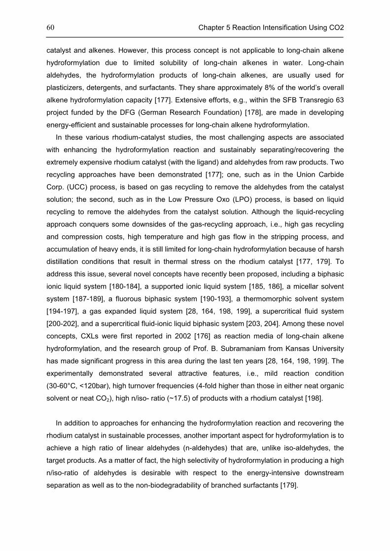
60 Chapter 5 Reaction Intensification Using CO2
catalyst and alkenes. However, this process concept is not applicable to long-chain alkene
hydroformylation due to limited solubility of long-chain alkenes in water. Long-chain
aldehydes, the hydroformylation products of long-chain alkenes, are usually used for
plasticizers, detergents, and surfactants. They share approximately 8% of the world’s overall
alkene hydroformylation capacity [177]. Extensive efforts, e.g., within the SFB Transregio 63
project funded by the DFG (German Research Foundation) [178], are made in developing
energy-efficient and sustainable processes for long-chain alkene hydroformylation.
In these various rhodium-catalyst studies, the most challenging aspects are associated
with enhancing the hydroformylation reaction and sustainably separating/recovering the
extremely expensive rhodium catalyst (with the ligand) and aldehydes from raw products. Two
recycling approaches have been demonstrated [177]; one, such as in the Union Carbide
Corp. (UCC) process, is based on gas recycling to remove the aldehydes from the catalyst
solution; the second, such as in the Low Pressure Oxo (LPO) process, is based on liquid
recycling to remove the aldehydes from the catalyst solution. Although the liquid-recycling
approach conquers some downsides of the gas-recycling approach, i.e., high gas recycling
and compression costs, high temperature and high gas flow in the stripping process, and
accumulation of heavy ends, it is still limited for long-chain hydroformylation because of harsh
distillation conditions that result in thermal stress on the rhodium catalyst [177, 179]. To
address this issue, several novel concepts have recently been proposed, including a biphasic
ionic liquid system [180-184], a supported ionic liquid system [185, 186], a micellar solvent
system [187-189], a fluorous biphasic system [190-193], a thermomorphic solvent system
[194-197], a gas expanded liquid system [28, 164, 198, 199], a supercritical fluid system
[200-202], and a supercritical fluid-ionic liquid biphasic system [203, 204]. Among these novel
concepts, CXLs were first reported in 2002 [176] as reaction media of long-chain alkene
hydroformylation, and the research group of Prof. B. Subramaniam from Kansas University
has made significant progress in this area during the last ten years [28, 164, 198, 199]. The
experimentally demonstrated several attractive features, i.e., mild reaction condition
(30-60°C, <120bar), high turnover frequencies (4-fold higher than those in either neat organic
solvent or neat CO2), high n/iso- ratio (~17.5) of products with a rhodium catalyst [198].
In addition to approaches for enhancing the hydroformylation reaction and recovering the
rhodium catalyst in sustainable processes, another important aspect for hydroformylation is to
achieve a high ratio of linear aldehydes (n-aldehydes) that are, unlike iso-aldehydes, the
target products. As a matter of fact, the high selectivity of hydroformylation in producing a high
n/iso-ratio of aldehydes is desirable with respect to the energy-intensive downstream
separation as well as to the non-biodegradability of branched surfactants [179].
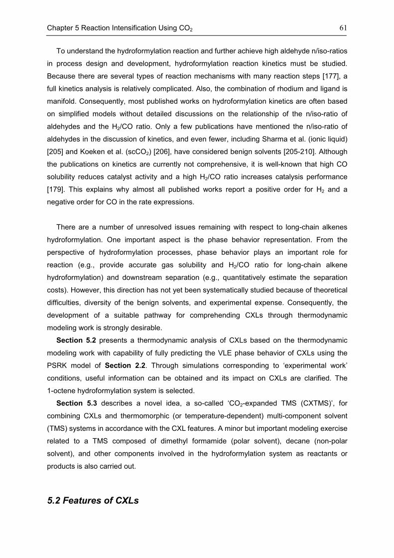
Chapter 5 Reaction Intensification Using CO2 61
To understand the hydroformylation reaction and further achieve high aldehyde n/iso-ratios
in process design and development, hydroformylation reaction kinetics must be studied.
Because there are several types of reaction mechanisms with many reaction steps [177], a
full kinetics analysis is relatively complicated. Also, the combination of rhodium and ligand is
manifold. Consequently, most published works on hydroformylation kinetics are often based
on simplified models without detailed discussions on the relationship of the n/iso-ratio of
aldehydes and the H2/CO ratio. Only a few publications have mentioned the n/iso-ratio of
aldehydes in the discussion of kinetics, and even fewer, including Sharma et al. (ionic liquid)
[205] and Koeken et al. (scCO2) [206], have considered benign solvents [205-210]. Although
the publications on kinetics are currently not comprehensive, it is well-known that high CO
solubility reduces catalyst activity and a high H2/CO ratio increases catalysis performance
[179]. This explains why almost all published works report a positive order for H2 and a
negative order for CO in the rate expressions.
There are a number of unresolved issues remaining with respect to long-chain alkenes
hydroformylation. One important aspect is the phase behavior representation. From the
perspective of hydroformylation processes, phase behavior plays an important role for
reaction (e.g., provide accurate gas solubility and H2/CO ratio for long-chain alkene
hydroformylation) and downstream separation (e.g., quantitatively estimate the separation
costs). However, this direction has not yet been systematically studied because of theoretical
difficulties, diversity of the benign solvents, and experimental expense. Consequently, the
development of a suitable pathway for comprehending CXLs through thermodynamic
modeling work is strongly desirable.
Section 5.2 presents a thermodynamic analysis of CXLs based on the thermodynamic
modeling work with capability of fully predicting the VLE phase behavior of CXLs using the
PSRK model of Section 2.2. Through simulations corresponding to ‘experimental work’
conditions, useful information can be obtained and its impact on CXLs are clarified. The
1-octene hydroformylation system is selected.
Section 5.3 describes a novel idea, a so-called ‘CO2-expanded TMS (CXTMS)’, for
combining CXLs and thermomorphic (or temperature-dependent) multi-component solvent
(TMS) systems in accordance with the CXL features. A minor but important modeling exercise
related to a TMS composed of dimethyl formamide (polar solvent), decane (non-polar
solvent), and other components involved in the hydroformylation system as reactants or
products is also carried out.
5.2 Features of CXLs
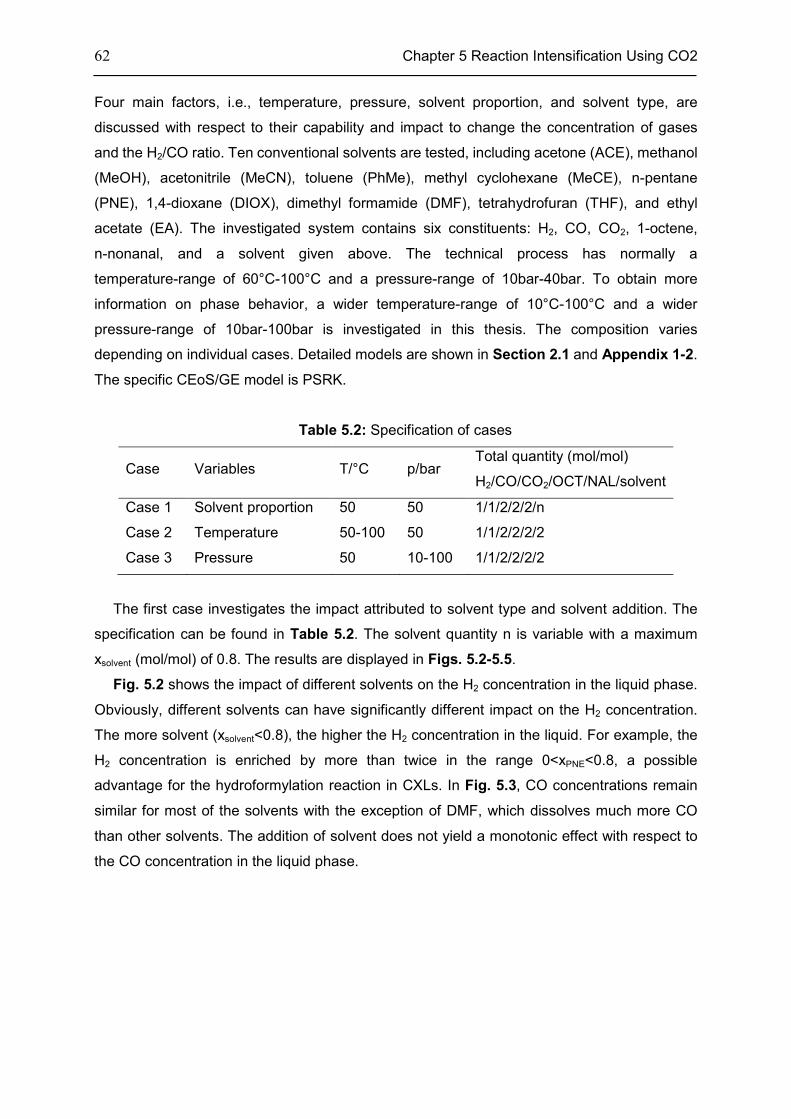
62 Chapter 5 Reaction Intensification Using CO2
Four main factors, i.e., temperature, pressure, solvent proportion, and solvent type, are
discussed with respect to their capability and impact to change the concentration of gases
and the H2/CO ratio. Ten conventional solvents are tested, including acetone (ACE), methanol
(MeOH), acetonitrile (MeCN), toluene (PhMe), methyl cyclohexane (MeCE), n-pentane
(PNE), 1,4-dioxane (DIOX), dimethyl formamide (DMF), tetrahydrofuran (THF), and ethyl
acetate (EA). The investigated system contains six constituents: H2, CO, CO2, 1-octene,
n-nonanal, and a solvent given above. The technical process has normally a
temperature-range of 60°C-100°C and a pressure-range of 10bar-40bar. To obtain more
information on phase behavior, a wider temperature-range of 10°C-100°C and a wider
pressure-range of 10bar-100bar is investigated in this thesis. The composition varies
depending on individual cases. Detailed models are shown in Section 2.1 and Appendix 1-2.
The specific CEoS/GE model is PSRK.
Table 5.2: Specification of cases
Case Variables T/°C p/bar Total quantity (mol/mol)
H2/CO/CO2/OCT/NAL/solvent
Case 1 Solvent proportion 50 50 1/1/2/2/2/n
Case 2 Temperature 50-100 50 1/1/2/2/2/2
Case 3 Pressure 50 10-100 1/1/2/2/2/2
The first case investigates the impact attributed to solvent type and solvent addition. The
specification can be found in Table 5.2. The solvent quantity n is variable with a maximum
xsolvent (mol/mol) of 0.8. The results are displayed in Figs. 5.2-5.5.
Fig. 5.2 shows the impact of different solvents on the H2 concentration in the liquid phase.
Obviously, different solvents can have significantly different impact on the H2 concentration.
The more solvent (xsolvent<0.8), the higher the H2 concentration in the liquid. For example, the
H2 concentration is enriched by more than twice in the range 0<xPNE<0.8, a possible
advantage for the hydroformylation reaction in CXLs. In Fig. 5.3, CO concentrations remain
similar for most of the solvents with the exception of DMF, which dissolves much more CO
than other solvents. The addition of solvent does not yield a monotonic effect with respect to
the CO concentration in the liquid phase.
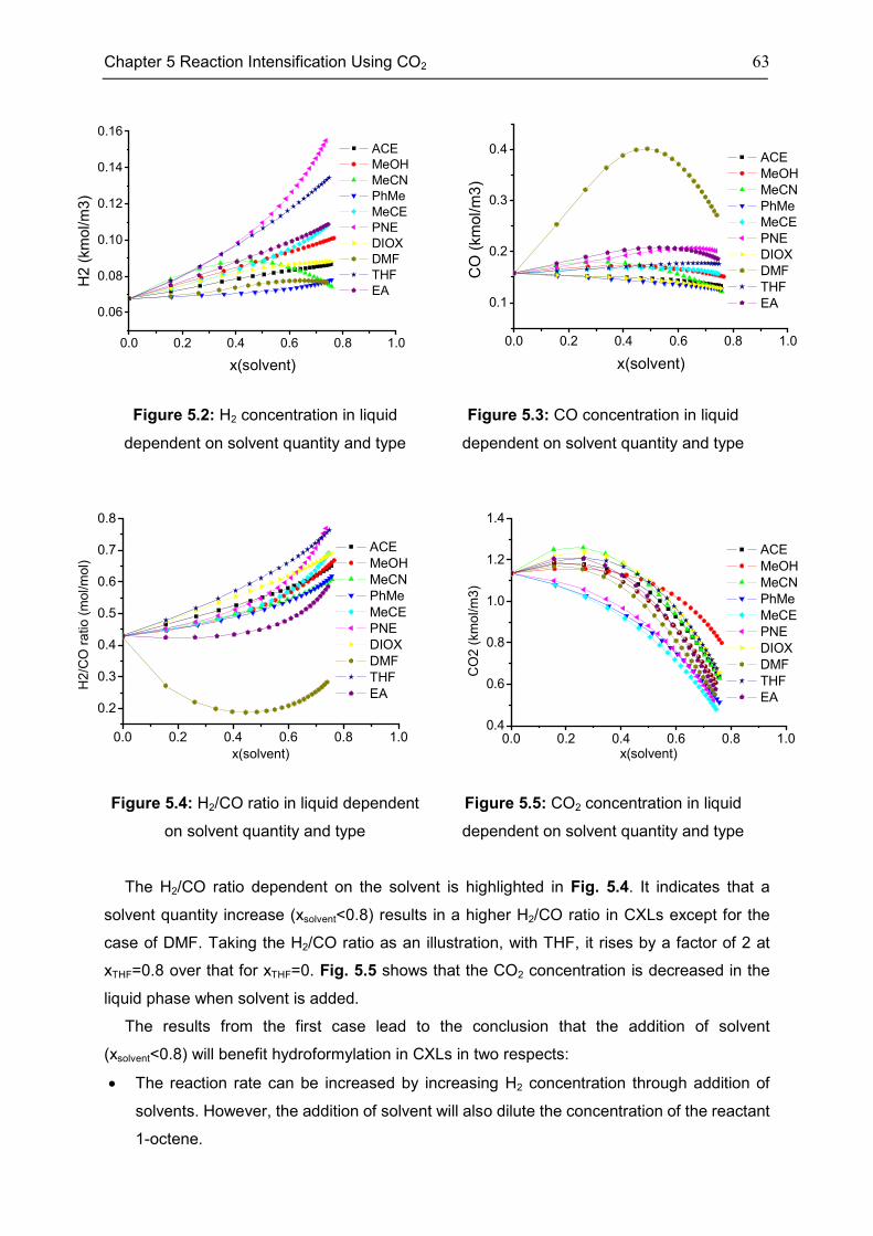
Chapter 5 Reaction Intensification Using CO2 63
Figure 5.2: H2 concentration in liquid
dependent on solvent quantity and type
Figure 5.3: CO concentration in liquid
dependent on solvent quantity and type
Figure 5.4: H2/CO ratio in liquid dependent
on solvent quantity and type
Figure 5.5: CO2 concentration in liquid
dependent on solvent quantity and type
The H2/CO ratio dependent on the solvent is highlighted in Fig. 5.4. It indicates that a
solvent quantity increase (xsolvent<0.8) results in a higher H2/CO ratio in CXLs except for the
case of DMF. Taking the H2/CO ratio as an illustration, with THF, it rises by a factor of 2 at
xTHF=0.8 over that for xTHF=0. Fig. 5.5 shows that the CO2 concentration is decreased in the
liquid phase when solvent is added.
The results from the first case lead to the conclusion that the addition of solvent
(xsolvent<0.8) will benefit hydroformylation in CXLs in two respects:
• The reaction rate can be increased by increasing H2 concentration through addition of
solvents. However, the addition of solvent will also dilute the concentration of the reactant
1-octene.
0.0 0.2 0.4 0.6 0.8 1.0
0.06
0.08
0.10
0.12
0.14
0.16
ACE
MeOH
MeCN
PhMe
MeCE
PNE
DIOX
DMF
THF
EA
H2
(km
ol/m
3)
x(solvent)
0.0 0.2 0.4 0.6 0.8 1.0
0.1
0.2
0.3
0.4 ACE
MeOH
MeCN
PhMe
MeCE
PNE
DIOX
DMF
THF
EA
CO
(km
ol/m
3)
x(solvent)
0.0 0.2 0.4 0.6 0.8 1.0
0.2
0.3
0.4
0.5
0.6
0.7
0.8
ACE
MeOH
MeCN
PhMe
MeCE
PNE
DIOX
DMF
THF
EA
H2/C
O r
atio (
mol/m
ol)
x(solvent)0.0 0.2 0.4 0.6 0.8 1.0
0.4
0.6
0.8
1.0
1.2
1.4
ACE
MeOH
MeCN
PhMe
MeCE
PNE
DIOX
DMF
THF
EA
CO
2 (
km
ol/m
3)
x(solvent)
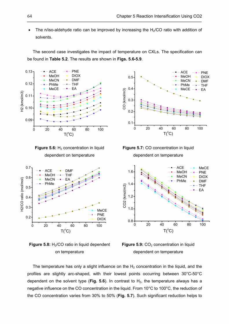
64 Chapter 5 Reaction Intensification Using CO2
• The n/iso-aldehyde ratio can be improved by increasing the H2/CO ratio with addition of
solvents.
The second case investigates the impact of temperature on CXLs. The specification can
be found in Table 5.2. The results are shown in Figs. 5.6-5.9.
Figure 5.6: H2 concentration in liquid
dependent on temperature
Figure 5.7: CO concentration in liquid
dependent on temperature
Figure 5.8: H2/CO ratio in liquid dependent
on temperature
Figure 5.9: CO2 concentration in liquid
dependent on temperature
The temperature has only a slight influence on the H2 concentration in the liquid, and the
profiles are slightly arc-shaped, with their lowest points occurring between 30°C-50°C
dependent on the solvent type (Fig. 5.6). In contrast to H2, the temperature always has a
negative influence on the CO concentration in the liquid. From 10°C to 100°C, the reduction of
the CO concentration varies from 30% to 50% (Fig. 5.7). Such significant reduction helps to
0 20 40 60 80 100
0.09
0.10
0.11
0.12
0.13 PNE
DIOX
DMF
THF
EA
ACE
MeOH
MeCN
PhMe
MeCE
H2 (
km
ol/m
3)
T(oC)
0 20 40 60 80 100
0.1
0.2
0.3
0.4
0.5
T(oC)
PNE
DIOX
DMF
THF
EA
ACE
MeOH
MeCN
PhMe
MeCE
CO
(km
ol/m
3)
0 20 40 60 80 100
0.2
0.3
0.4
0.5
0.6
0.7 DMF
THF
EA
H2/C
O r
atio (
mol/m
ol)
T(oC)
MeCE
PNE
DIOX
ACE
MeOH
MeCN
PhMe
0 20 40 60 80 1000.8
1.0
1.2
1.4
1.6 MeCE
PNE
DIOX
DMF
THF
EA
ACE
MeOH
MeCN
PhMe
CO
2 (
km
ol/m
3)
T(oC)
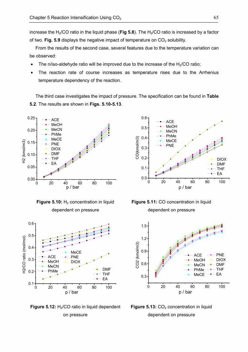
Chapter 5 Reaction Intensification Using CO2 65
increase the H2/CO ratio in the liquid phase (Fig 5.8). The H2/CO ratio is increased by a factor
of two. Fig. 5.9 displays the negative impact of temperature on CO2 solubility.
From the results of the second case, several features due to the temperature variation can
be observed:
• The n/iso-aldehyde ratio will be improved due to the increase of the H2/CO ratio;
• The reaction rate of course increases as temperature rises due to the Arrhenius
temperature dependency of the reaction.
The third case investigates the impact of pressure. The specification can be found in Table
5.2. The results are shown in Figs. 5.10-5.13.
Figure 5.10: H2 concentration in liquid
dependent on pressure
Figure 5.11: CO concentration in liquid
dependent on pressure
Figure 5.12: H2/CO ratio in liquid dependent
on pressure
Figure 5.13: CO2 concentration in liquid
dependent on pressure
0 20 40 60 80 1000.00
0.05
0.10
0.15
0.20
0.25 ACE
MeOH
MeCN
PhMe
MeCE
PNE
DIOX
DMF
THF
EA
p / bar
H2
(km
ol/m
3)
0 20 40 60 80 1000.0
0.1
0.2
0.3
0.4
0.5
0.6
DIOX
DMF
THF
EA
p / bar
ACE
MeOH
MeCN
PhMe
MeCE
PNE
CO
(km
ol/m
3)
0 20 40 60 80 1000.1
0.2
0.3
0.4
0.5
0.6
MeCE
PNE
DIOX
p / bar
DMF
THF
EA
ACE
MeOH
MeCN
PhMeH2/C
O r
atio (
mol/m
ol)
0 20 40 60 80 100
0.3
0.6
0.9
1.2
1.5
p / bar
PNE
DIOX
DMF
THF
EA
ACE
MeOH
MeCN
PhMe
MeCE
CO
2 (
km
ol/m
3)
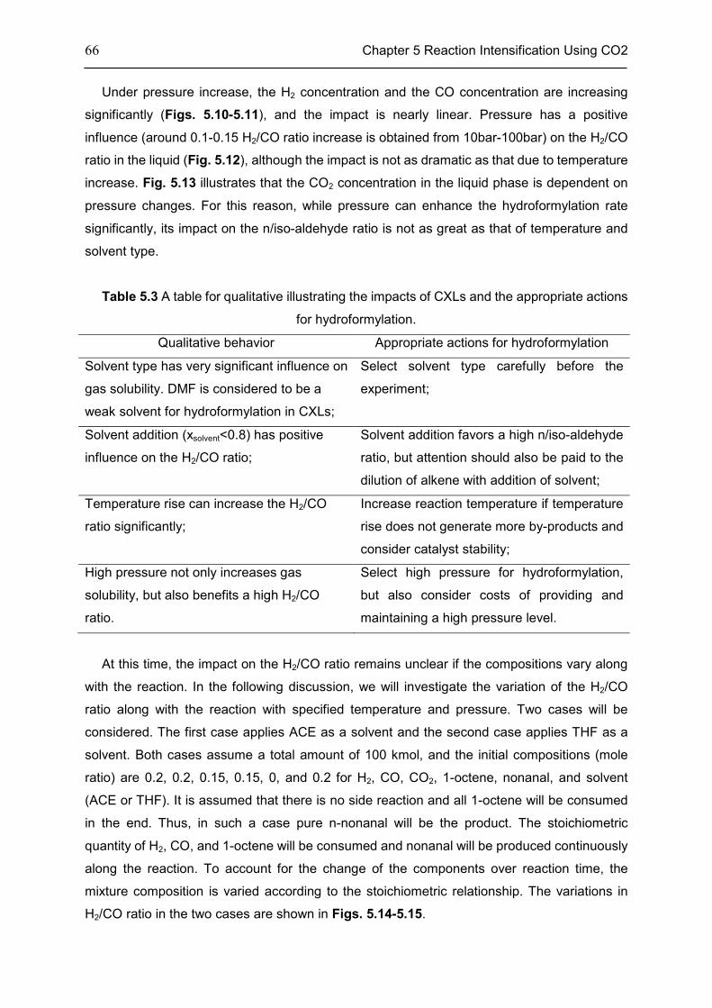
66 Chapter 5 Reaction Intensification Using CO2
Under pressure increase, the H2 concentration and the CO concentration are increasing
significantly (Figs. 5.10-5.11), and the impact is nearly linear. Pressure has a positive
influence (around 0.1-0.15 H2/CO ratio increase is obtained from 10bar-100bar) on the H2/CO
ratio in the liquid (Fig. 5.12), although the impact is not as dramatic as that due to temperature
increase. Fig. 5.13 illustrates that the CO2 concentration in the liquid phase is dependent on
pressure changes. For this reason, while pressure can enhance the hydroformylation rate
significantly, its impact on the n/iso-aldehyde ratio is not as great as that of temperature and
solvent type.
Table 5.3 A table for qualitative illustrating the impacts of CXLs and the appropriate actions
for hydroformylation.
Qualitative behavior Appropriate actions for hydroformylation
Solvent type has very significant influence on
gas solubility. DMF is considered to be a
weak solvent for hydroformylation in CXLs;
Select solvent type carefully before the
experiment;
Solvent addition (xsolvent<0.8) has positive
influence on the H2/CO ratio;
Solvent addition favors a high n/iso-aldehyde
ratio, but attention should also be paid to the
dilution of alkene with addition of solvent;
Temperature rise can increase the H2/CO
ratio significantly;
Increase reaction temperature if temperature
rise does not generate more by-products and
consider catalyst stability;
High pressure not only increases gas
solubility, but also benefits a high H2/CO
ratio.
Select high pressure for hydroformylation,
but also consider costs of providing and
maintaining a high pressure level.
At this time, the impact on the H2/CO ratio remains unclear if the compositions vary along
with the reaction. In the following discussion, we will investigate the variation of the H2/CO
ratio along with the reaction with specified temperature and pressure. Two cases will be
considered. The first case applies ACE as a solvent and the second case applies THF as a
solvent. Both cases assume a total amount of 100 kmol, and the initial compositions (mole
ratio) are 0.2, 0.2, 0.15, 0.15, 0, and 0.2 for H2, CO, CO2, 1-octene, nonanal, and solvent
(ACE or THF). It is assumed that there is no side reaction and all 1-octene will be consumed
in the end. Thus, in such a case pure n-nonanal will be the product. The stoichiometric
quantity of H2, CO, and 1-octene will be consumed and nonanal will be produced continuously
along the reaction. To account for the change of the components over reaction time, the
mixture composition is varied according to the stoichiometric relationship. The variations in
H2/CO ratio in the two cases are shown in Figs. 5.14-5.15.
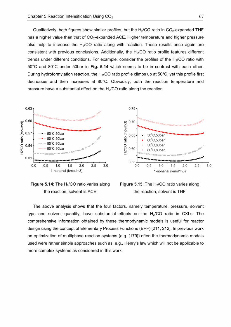
Chapter 5 Reaction Intensification Using CO2 67
Qualitatively, both figures show similar profiles, but the H2/CO ratio in CO2-expanded THF
has a higher value than that of CO2-expanded ACE. Higher temperature and higher pressure
also help to increase the H2/CO ratio along with reaction. These results once again are
consistent with previous conclusions. Additionally, the H2/CO ratio profile features different
trends under different conditions. For example, consider the profiles of the H2/CO ratio with
50°C and 80°C under 50bar in Fig. 5.14 which seems to be in contrast with each other.
During hydroformylation reaction, the H2/CO ratio profile climbs up at 50°C, yet this profile first
decreases and then increases at 80°C. Obviously, both the reaction temperature and
pressure have a substantial effect on the H2/CO ratio along the reaction.
Figure 5.14: The H2/CO ratio varies along
the reaction, solvent is ACE
Figure 5.15: The H2/CO ratio varies along
the reaction, solvent is THF
The above analysis shows that the four factors, namely temperature, pressure, solvent
type and solvent quantity, have substantial effects on the H2/CO ratio in CXLs. The
comprehensive information obtained by these thermodynamic models is useful for reactor
design using the concept of Elementary Process Functions (EPF) [211, 212]. In previous work
on optimization of multiphase reaction systems (e.g. [179]) often the thermodynamic models
used were rather simple approaches such as, e.g., Henry’s law which will not be applicable to
more complex systems as considered in this work.
0.0 0.5 1.0 1.5 2.0 2.5 3.0
0.51
0.54
0.57
0.60
0.63
H2
/CO
ra
tio (
mol/m
ol)
1-nonanal (kmol/m3)
50oC,50bar
80oC,50bar
50oC,80bar
80oC,80bar
0.0 0.5 1.0 1.5 2.0 2.5 3.00.55
0.60
0.65
0.70
0.75
H2/C
O r
atio (
mo
l/m
ol)
1-nonanal (kmol/m3)
50oC,50bar
80oC,50bar
50oC,80bar
80oC,80bar

68 Chapter 5 Reaction Intensification Using CO2
5.3 CO2-Expanded TMS
Figure 5.16: Publication review of TMS and hydroformylation in TMS (inquired by SCOPUS
with temperature-dependent multi-component solvent or thermomorphic multi-component
solvent and hydroformylation in title or abstract or keyword)
Pioneering work on TMS systems has been carried out by the group of Prof. A. Behr from
TU Dortmund since 2005 [213]. There are only few publications, a total of 17 (Fig. 5.16), and
a considerable number of them deal with the application of TMS for a hydroformylation
reaction system. Obviously, the TMS system offers specific advantages for product
separation as well as for catalyst recovery [214], and, as discussed in Chapter 1 and
Sections 5.1-5.2, CXLs provide benefits to the hydroformylation reaction in several aspects
(Table 5.3). If these two concepts are particularly integrated into the reaction and into
separation, the integrated process could be extremely efficient. Technically speaking, this
concept is possible, because both constituents of TMS, dimethyl formamide (DMF) and
n-decane (C10), can be efficiently expanded [215, 216].
Table 5.4: Features of CXTMS and possible benefits for the hydroformylation process
Feature Possible benefit
Enhance solubility of gases Increase reaction rate, reduce reactor size
Increase H2/CO ratio Increase n/iso-aldehyde ratio in the product
Enhanced transport rates Increase reaction rate, reduce reactor size
Eco-friendly feature Reduce pollution
The LLE information may be used to design the operational point between reaction and
downstream separation of hydroformylation in TMS. Therefore, the thermodynamic modeling
of this complex system is an important part of the SFB Transregio 63 project [178], especially
2004 2006 2008 2010 2012 20140
1
2
3
4
5
Nu
mb
er
of
pub
lica
tion
s
Year
TMS
Hydroformylation in TMS
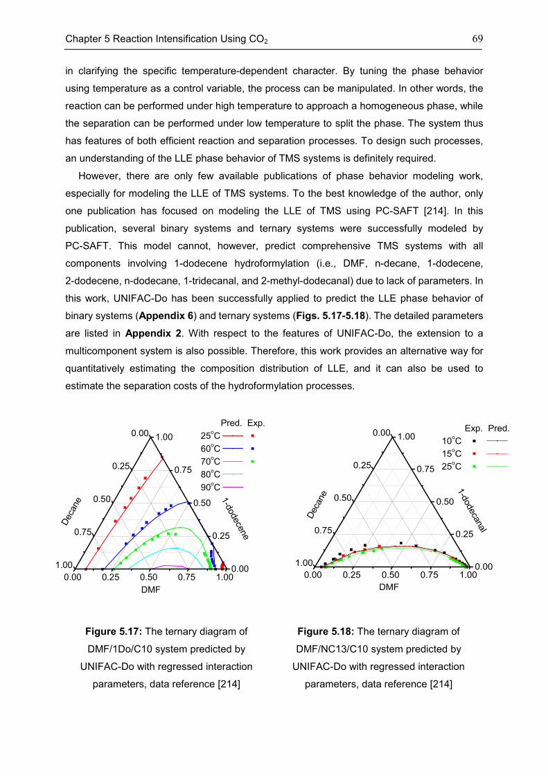
Chapter 5 Reaction Intensification Using CO2 69
in clarifying the specific temperature-dependent character. By tuning the phase behavior
using temperature as a control variable, the process can be manipulated. In other words, the
reaction can be performed under high temperature to approach a homogeneous phase, while
the separation can be performed under low temperature to split the phase. The system thus
has features of both efficient reaction and separation processes. To design such processes,
an understanding of the LLE phase behavior of TMS systems is definitely required.
However, there are only few available publications of phase behavior modeling work,
especially for modeling the LLE of TMS systems. To the best knowledge of the author, only
one publication has focused on modeling the LLE of TMS using PC-SAFT [214]. In this
publication, several binary systems and ternary systems were successfully modeled by
PC-SAFT. This model cannot, however, predict comprehensive TMS systems with all
components involving 1-dodecene hydroformylation (i.e., DMF, n-decane, 1-dodecene,
2-dodecene, n-dodecane, 1-tridecanal, and 2-methyl-dodecanal) due to lack of parameters. In
this work, UNIFAC-Do has been successfully applied to predict the LLE phase behavior of
binary systems (Appendix 6) and ternary systems (Figs. 5.17-5.18). The detailed parameters
are listed in Appendix 2. With respect to the features of UNIFAC-Do, the extension to a
multicomponent system is also possible. Therefore, this work provides an alternative way for
quantitatively estimating the composition distribution of LLE, and it can also be used to
estimate the separation costs of the hydroformylation processes.
Figure 5.17: The ternary diagram of
DMF/1Do/C10 system predicted by
UNIFAC-Do with regressed interaction
parameters, data reference [214]
Figure 5.18: The ternary diagram of
DMF/NC13/C10 system predicted by
UNIFAC-Do with regressed interaction
parameters, data reference [214]
0.00 0.25 0.50 0.75 1.000.00
0.25
0.50
0.75
1.000.00
0.25
0.50
0.75
1.00
1-d
odece
ne
Pred. Exp.
25oC
60oC
70oC
80oC
90oC
Deca
ne
DMF
0.00 0.25 0.50 0.75 1.000.00
0.25
0.50
0.75
1.000.00
0.25
0.50
0.75
1.00
1-d
odeca
nal
Exp. Pred.
10oC
15oC
25oC
Deca
ne
DMF
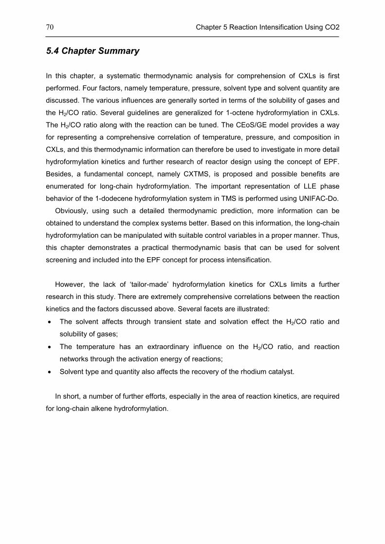
70 Chapter 5 Reaction Intensification Using CO2
5.4 Chapter Summary
In this chapter, a systematic thermodynamic analysis for comprehension of CXLs is first
performed. Four factors, namely temperature, pressure, solvent type and solvent quantity are
discussed. The various influences are generally sorted in terms of the solubility of gases and
the H2/CO ratio. Several guidelines are generalized for 1-octene hydroformylation in CXLs.
The H2/CO ratio along with the reaction can be tuned. The CEoS/GE model provides a way
for representing a comprehensive correlation of temperature, pressure, and composition in
CXLs, and this thermodynamic information can therefore be used to investigate in more detail
hydroformylation kinetics and further research of reactor design using the concept of EPF.
Besides, a fundamental concept, namely CXTMS, is proposed and possible benefits are
enumerated for long-chain hydroformylation. The important representation of LLE phase
behavior of the 1-dodecene hydroformylation system in TMS is performed using UNIFAC-Do.
Obviously, using such a detailed thermodynamic prediction, more information can be
obtained to understand the complex systems better. Based on this information, the long-chain
hydroformylation can be manipulated with suitable control variables in a proper manner. Thus,
this chapter demonstrates a practical thermodynamic basis that can be used for solvent
screening and included into the EPF concept for process intensification.
However, the lack of ‘tailor-made’ hydroformylation kinetics for CXLs limits a further
research in this study. There are extremely comprehensive correlations between the reaction
kinetics and the factors discussed above. Several facets are illustrated:
• The solvent affects through transient state and solvation effect the H2/CO ratio and
solubility of gases;
• The temperature has an extraordinary influence on the H2/CO ratio, and reaction
networks through the activation energy of reactions;
• Solvent type and quantity also affects the recovery of the rhodium catalyst.
In short, a number of further efforts, especially in the area of reaction kinetics, are required
for long-chain alkene hydroformylation.
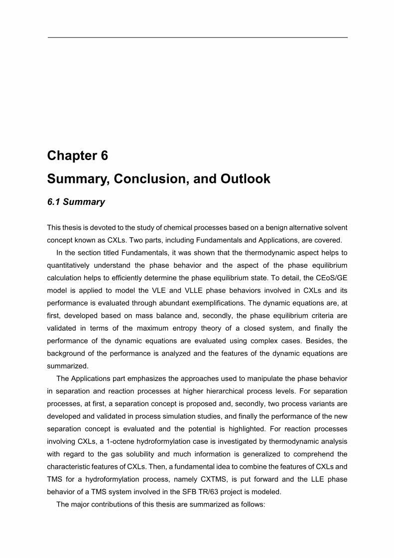
Chapter 6
Summary, Conclusion, and Outlook
6.1 Summary
This thesis is devoted to the study of chemical processes based on a benign alternative solvent
concept known as CXLs. Two parts, including Fundamentals and Applications, are covered.
In the section titled Fundamentals, it was shown that the thermodynamic aspect helps to
quantitatively understand the phase behavior and the aspect of the phase equilibrium
calculation helps to efficiently determine the phase equilibrium state. To detail, the CEoS/GE
model is applied to model the VLE and VLLE phase behaviors involved in CXLs and its
performance is evaluated through abundant exemplifications. The dynamic equations are, at
first, developed based on mass balance and, secondly, the phase equilibrium criteria are
validated in terms of the maximum entropy theory of a closed system, and finally the
performance of the dynamic equations are evaluated using complex cases. Besides, the
background of the performance is analyzed and the features of the dynamic equations are
summarized.
The Applications part emphasizes the approaches used to manipulate the phase behavior
in separation and reaction processes at higher hierarchical process levels. For separation
processes, at first, a separation concept is proposed and, secondly, two process variants are
developed and validated in process simulation studies, and finally the performance of the new
separation concept is evaluated and the potential is highlighted. For reaction processes
involving CXLs, a 1-octene hydroformylation case is investigated by thermodynamic analysis
with regard to the gas solubility and much information is generalized to comprehend the
characteristic features of CXLs. Then, a fundamental idea to combine the features of CXLs and
TMS for a hydroformylation process, namely CXTMS, is put forward and the LLE phase
behavior of a TMS system involved in the SFB TR/63 project is modeled.
The major contributions of this thesis are summarized as follows:
72 Chapter 6 Summary, Conclusion, and Outlook
• Provided practical path to model the phase behavior (VLE and VLLE) of CXLs using the
CEoS/GE models, and phase behavior (LLE) of TMS using UNIFAC-Do;
• Established the dynamic equations to determine phase behavior equilibria;
• Designed and validated a new concept to separate azeotropic mixtures;
• Studied the hydroformylation in CXLs using a thermodynamic method.
6.2 Conclusion
After this study, a general conclusion can be drawn that a clear route from the phase level to
the unit operation level and/or plant level can be established. The implementation from the
phase level to the higher hierarchical levels (unit operation level and/or plant level) is
successfully performed.
The Fundamentals part confirms the capacity of the CEoS/GE model to predict the VLE and
VLLE phase behaviors of CXLs and the practical characters of dynamic equations to
determine phase behaviors. Therefore, this identification of phase equilibria provides a
confident basis to implement the phase level to higher hierarchical levels. To detail the
thermodynamic modeling work, the CEoS/GE model is practical to provide VLE information of
CXLs with regard to the feature of UNIFAC, in case without experimental data. But, a
CEoS/GE model with adjustable parameters is required for a good prediction of the VLLE
phase behavior. Therefore, experimental data are consequently required for parameter
estimation. On another hand, the dynamic equations demonstrated as novel but general
approach provide the practical benefits to determine complex phase equilibria.
In the Applications part, the implementation from the phase level to the higher hierarchical
levels is exemplified in an azeotropic mixture separation process in particular. The results
show that the new chemical process employing the benign alternatives is significantly different
in comparison to the conventional chemical processes and that it has significant potential for
process intensification. Therefore, the novel separation concept is a promising alternative to
the conventional processes for azeotropic mixture separation. For reaction intensification
using CO2, though there is no suitable kinetics to quantitatively implement reaction from the
phase level to the higher hierarchical levels as in the separation case, the thermodynamic
analysis provides a path to comprehend the 1-octene hydroformylation system in CXLs, and
the thermodynamic modeling of 1-dodecene hydroformylation system in TMS expresses the
phase behavior tuning between homogeneous reaction and heterogeneous separation
quantitatively. Therefore, this provides a suitable path to implement the phase level to the
higher hierarchical levels with respect to downstream separation. The hypothesis, CXTMS, is
still required to be validated through experiments.
Chapter 6 Summary, Conclusion, and Outlook 73
6.3 Outlook
Due to complexity of the benign solvent alternatives, further work is required to expand upon
several points not covered in this thesis.
In the first place, more experimental work is required to be able to study the phase
behavior of CXLs more in depth. Especially the VLLE phase behavior of CXLs systems
cannot be fully predicted without any data. Moreover, only a few binary systems regarding the
‘salting-out’ performance have been published. Unfortunately, this data is still not totally
acceptable on accounts of the disagreement in different publications due to difficulty of
complex phase behavior measurement. On this point there is still wide open space to explore.
In another word, the powerful models are also still necessary to be used for predicting the
phase behavior in case of limited data or even no data. For instance, in Chapter 4, the PRWS
with regressed kij from isothermal data can have high uncertainties when extrapolated to other
temperatures. So currently, only the influence of pressure on the process is clarified; the
influence of temperature on the process remains unknown. If the temperature can be included
in modeling, the dimension of thermodynamic space for the process is much greater, and
better solutions may be found.
Quite a few facets of research on the long-chain alkene hydroformylation have to be
comprehensively manipulated, i.e., thermodynamic aspect, reaction kinetics and catalyst
recovery. Several bottlenecks still require much effort:
• Prediction of the phase behavior involving benign solvents. It is difficult if ILs or surfactants
are involved because there is no credible method for them. If the system is more complex,
e.g., scCO2 + ILs, the research has been only carried out empirically;
• Prediction of the reaction rate with respect to solvents, as solvents may have a
non-negligible effect on reaction kinetics;
• Catalyst recovery. The rhodium catalyst is more expensive than gold, and it is not
acceptable in industry if the rhodium concentration in the raw product stream is more than
1-10ppb. This is a harsh constraint.
The dynamic approach for determining phase behavior shows practical ability. However,
the theoretical basis is based on a closed system with constant temperature and pressure. The
possibility to extend this method to the close/open system with reaction, with or without
unknown temperatures and pressures, is still an open topic.

Appendix
Appendix 1: CEoS/GE model
All CEoS/GE mixing rules are derived from the basic relationship between GE and φ:
( )( )
( )( )
*
. , ,
*
, . , .
, , ,ln ln
, , ,
EENCref m EoS i i EoSEoS
iim ref i i ref
G T p x T pGx
RT RT T p x T p
ϕ ϕ
ϕ ϕ− = −∑ (a1)
Usually, only two reference fluids are used, i.e., ideal fluid and VDW fluid (Table 2.1). Most of
mixing rules apply ideal fluid as reference, after that the Eq. (a1) is derived as:
( ) ( )lnE
NC NCEoS m mm i i m m i i ii i
i i
G Z BZ x Z C V x C V
RT Z Bε ε
−= − − − −
− ∑ ∑ (a2)
Or ( ) ( )lnE
NC NCEoS m mi m m i i ii i
i i
A Z Bx C V x C V
RT Z Bε ε
−= − − −
− ∑ ∑ (a3)
With 1
( ) lnV wb
C Vu w V ub
+ = − + ,
1 1* ln
1
wC
u w u
+ = − + ,
1lnr
r wC
w u r u
+ = − − + ,
Vr
b= ,
2 2
apA
R T= ,
bpB
RT= ,
a A
bRT Bε = = .
Applying the simplifications based on infinite pressure and/or zero pressure theory, the
relationships is founded between E
EoSG and EG , and EG is calculated by
lnN
E
i i
i
G RT x γ= ∑ , where γ i is usually provided by activity models.
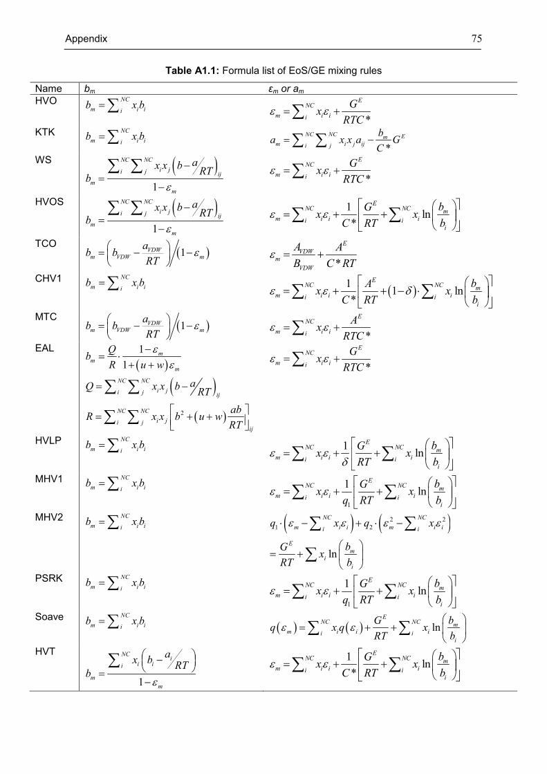
Appendix 75
Table A1.1: Formula list of EoS/GE mixing rules
Name bm εm or am
HVO NC
m i iib x b=∑
*
ENC
m i ii
Gx
RTCε ε= +∑
KTK NC
m i iib x b=∑
*
NC NC Emm i j iji j
ba x x a G
C= −∑ ∑
WS ( )1
NC NC
i ji j ij
m
m
ax x bRT
bε
−=
−
∑ ∑ *
ENC
m i ii
Gx
RTCε ε= +∑
HVOS ( )1
NC NC
i ji j ij
m
m
ax x bRT
bε
−=
−
∑ ∑
1ln
*
ENC NC m
m i i ii ii
bGx x
C RT bε ε
= + +
∑ ∑
TCO ( )1VDW
m VDW m
ab b
RTε = − −
*
E
VDWm
VDW
A A
B C RTε = +
CHV1 NC
m i iib x b=∑
( )11 ln
*
ENC NC m
m i i ii ii
bAx x
C RT bε ε δ
= + + − ⋅
∑ ∑
MTC ( )1VDW
m VDW m
ab b
RTε = − −
*
ENC
m i ii
Ax
RTCε ε= +∑
EAL
( )
( )( )2
1
1
mm
m
NC NC
i ji j ij
NC NC
i ji jij
Qb
R u w
aQ x x bRT
abR x x b u w
RT
εε
−= ⋅
+ +
= −
= + +
∑ ∑
∑ ∑
*
ENC
m i ii
Gx
RTCε ε= +∑
HVLP NC
m i iib x b=∑ 1
lnE
NC NC mm i i ii i
i
bGx x
RT bε ε
δ
= + +
∑ ∑
MHV1 NC
m i iib x b=∑
1
1ln
ENC NC m
m i i ii ii
bGx x
q RT bε ε
= + +
∑ ∑
MHV2 NC
m i iib x b=∑ ( ) ( )2 2
1 2
ln
NC NC
m i i m i ii i
E
mi
i
q x q x
bGx
RT b
ε ε ε ε⋅ − + ⋅ −
= +
∑ ∑
∑
PSRK NC
m i iib x b=∑
1
1ln
ENC NC m
m i i ii ii
bGx x
q RT bε ε
= + +
∑ ∑
Soave NC
m i iib x b=∑ ( ) ( ) ln
ENC NC m
m i i ii ii
bGq x q x
RT bε ε
= + +
∑ ∑
HVT
1
NCi
i ii
m
m
ax b
RTb
ε
− =−
∑
1ln
*
ENC NC m
m i i ii ii
bGx x
C RT bε ε
= + +
∑ ∑
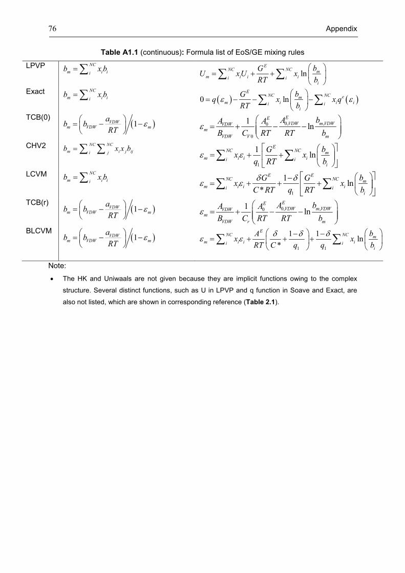
76 Appendix
Table A1.1 (continuous): Formula list of EoS/GE mixing rules
LPVP NC
m i iib x b=∑
lnE
NC NC mm i i ii i
i
bGU xU x
RT b
= + +
∑ ∑
Exact NC
m i iib x b=∑ ( ) ( )0 ln
ENC NC em
m i i ii ii
bGq x x q
RT bε ε
= − − −
∑ ∑
TCB(0) ( )1VDW
m VDW m
ab b
RTε = − −
0, ,0
0
1ln
EEVDW m VDWVDW
m
VDW V m
A bA A
B C RT RT bε
= + − −
CHV2 NC NC
m i j iji jb x x b=∑ ∑
1
1ln
ENC NC m
m i i ii ii
bGx x
q RT bε ε
= + +
∑ ∑
LCVM NC
m i iib x b=∑
1
1ln
*
E ENC NC m
m i i ii ii
bG Gx x
C RT q RT b
δ δε ε
−= + + +
∑ ∑
TCB(r) ( )1VDW
m VDW m
ab b
RTε = − −
0, ,01
ln
EEVDW m VDWVDW
m
VDW r m
A bA A
B C RT RT bε
= + − −
BLCVM ( )1VDW
m VDW m
ab b
RTε = − −
1 1
1 1ln
*
ENC NC m
m i i ii ii
bAx x
RT C q q b
δ δ δε ε
− −= + + +
∑ ∑
Note:
• The HK and Uniwaals are not given because they are implicit functions owing to the complex
structure. Several distinct functions, such as U in LPVP and q function in Soave and Exact, are
also not listed, which are shown in corresponding reference (Table 2.1).

Appendix 77
Appendix 2: Parameters of investigated systems
In this appendix, the parameters of modeling VLE and VLLE behavior of investigated system
are given. The detailed modeling steps are shown in [52, 83]. They contain:
• Table A2.1 shows the property parameters;
• Table A2.2 shows the interaction parameter kij of PRWS;
• Table A2.3-A2.5 shows the parameters of UNIFAC-PSRK and UNIFAC-Lby, which are
integrated in CEoS/GE models, see references [52, 83, 161];
• Table A2.6 shows the parameters for H2O/MeCN system (NRTL-IG) are obtained from
Aspen internal database [217];
• Table A2.7-A2.8 shows the parameters of UNIFAC-Do., which are used for predicting the
temperature dependent phase behavior of TMS system.
Table A2.1: Property parameters for various substances [217]
Component Tc/°C Pc (bar) ω Component Tc/°C Pc (bar) ω
H2O 373.98 220.55 0.344861 OCT 293.85 26.80 0.392059
MeOH 239.35 80.84 0.565831 NAL 384.85 27.30 0.511744
DME 126.95 53.70 0.200221 ACE 235.05 47.01 0.306527
CO2 31.06 73.83 0.223621 MeCN 272.35 48.30 0.337886
H2 -239.96 13.13 -0.21599 PhMe 318.60 41.08 0.264012
CO -140.23 34.99 0.048162 DIOX 313.85 52.081 0.279262
PNE 196.55 33.7 0.251506 MCH 298.95 34.8 0.236055
DMF 376.45 44.2 0.31771 EA 250.15 38.8 0.366409
MeCE 298.95 34.8 0.236055 THF 267 51.9 0.225354
Note:
• The parameters of Mathias-Copeman α function for MSRK and MPS are not given here,
details are shown in the article [52] or Aspen internal database [217].
Table A2.2: kij of PRWS model [52, 83, 161]
System Comp. i Comp. j PRWS, kij=kji (kii=0)
UNIFAC-PSRK UNIFAC-Lby NRTL
H2O/DIOX/CO2 H2O DIOX -- -- 0.088064
DIOX CO2 -- -- 0.278162
H2O CO2 -- -- 0.088064
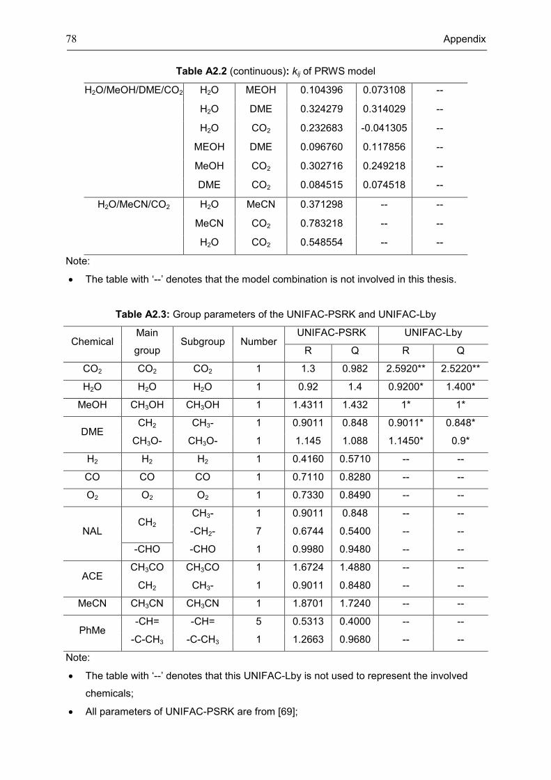
78 Appendix
Table A2.2 (continuous): kij of PRWS model
H2O/MeOH/DME/CO2 H2O MEOH 0.104396 0.073108 --
H2O DME 0.324279 0.314029 --
H2O CO2 0.232683 -0.041305 --
MEOH DME 0.096760 0.117856 --
MeOH CO2 0.302716 0.249218 --
DME CO2 0.084515 0.074518 --
H2O/MeCN/CO2 H2O MeCN 0.371298 -- --
MeCN CO2 0.783218 -- --
H2O CO2 0.548554 -- --
Note:
• The table with ‘--’ denotes that the model combination is not involved in this thesis.
Table A2.3: Group parameters of the UNIFAC-PSRK and UNIFAC-Lby
Chemical Main
group Subgroup Number
UNIFAC-PSRK UNIFAC-Lby
R Q R Q
CO2 CO2 CO2 1 1.3 0.982 2.5920** 2.5220**
H2O H2O H2O 1 0.92 1.4 0.9200* 1.400*
MeOH CH3OH CH3OH 1 1.4311 1.432 1* 1*
DME CH2 CH3- 1 0.9011 0.848 0.9011* 0.848*
CH3O- CH3O- 1 1.145 1.088 1.1450* 0.9*
H2 H2 H2 1 0.4160 0.5710 -- --
CO CO CO 1 0.7110 0.8280 -- --
O2 O2 O2 1 0.7330 0.8490 -- --
NAL CH2
CH3- 1 0.9011 0.848 -- --
-CH2- 7 0.6744 0.5400 -- --
-CHO -CHO 1 0.9980 0.9480 -- --
ACE CH3CO CH3CO 1 1.6724 1.4880 -- --
CH2 CH3- 1 0.9011 0.8480 -- --
MeCN CH3CN CH3CN 1 1.8701 1.7240 -- --
PhMe -CH= -CH= 5 0.5313 0.4000 -- --
-C-CH3 -C-CH3 1 1.2663 0.9680 -- --
Note:
• The table with ‘--’ denotes that this UNIFAC-Lby is not used to represent the involved
chemicals;
• All parameters of UNIFAC-PSRK are from [69];
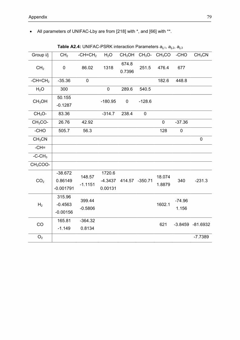
Appendix 79
• All parameters of UNIFAC-Lby are from [218] with *, and [66] with **.
Table A2.4: UNIFAC-PSRK interaction Parameters aij,1, aij,2, aij,3
Group i/j CH2 -CH=CH2 H2O CH3OH CH3O- CH3CO -CHO CH3CN
CH2 0 86.02 1318 674.8
0.7396 251.5 476.4 677
-CH=CH2 -35.36 0 182.6 448.8
H2O 300 0 289.6 540.5
CH3OH 50.155
-0.1287 -180.95 0 -128.6
CH3O- 83.36 -314.7 238.4 0
CH3CO- 26.76 42.92 0 -37.36
-CHO 505.7 56.3 128 0
CH3CN 0
-CH=
-C-CH3
CH3COO-
CO2
-38.672
0.86149
-0.001791
148.57
-1.1151
1720.6
-4.3437
0.00131
414.57 -350.71 18.074
1.8879 340 -231.3
H2
315.96
-0.4563
-0.00156
399.44
-0.5806 1602.1
-74.96
1.156
CO 165.81
-1.149
-364.32
0.8134 621 -3.8459 -81.6932
O2 -7.7389
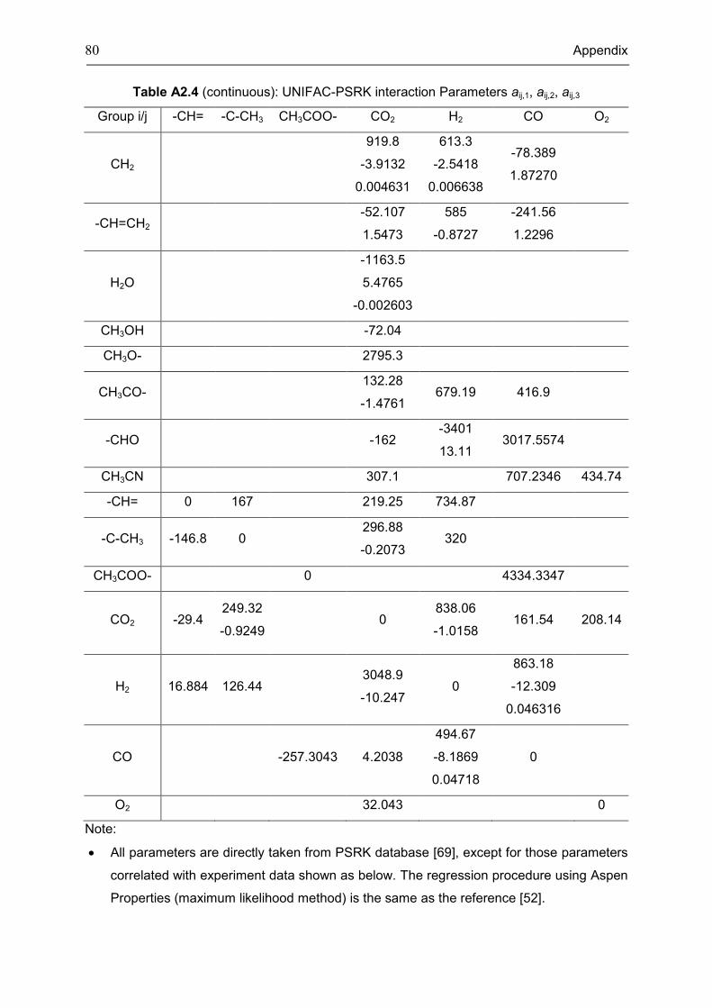
80 Appendix
Table A2.4 (continuous): UNIFAC-PSRK interaction Parameters aij,1, aij,2, aij,3
Group i/j -CH= -C-CH3 CH3COO- CO2 H2 CO O2
CH2
919.8
-3.9132
0.004631
613.3
-2.5418
0.006638
-78.389
1.87270
-CH=CH2 -52.107
1.5473
585
-0.8727
-241.56
1.2296
H2O
-1163.5
5.4765
-0.002603
CH3OH -72.04
CH3O- 2795.3
CH3CO- 132.28
-1.4761 679.19 416.9
-CHO -162 -3401
13.11 3017.5574
CH3CN 307.1 707.2346 434.74
-CH= 0 167 219.25 734.87
-C-CH3 -146.8 0 296.88
-0.2073 320
CH3COO- 0 4334.3347
CO2 -29.4 249.32
-0.9249 0
838.06
-1.0158 161.54 208.14
H2 16.884 126.44 3048.9
-10.247 0
863.18
-12.309
0.046316
CO -257.3043 4.2038
494.67
-8.1869
0.04718
0
O2 32.043 0
Note:
• All parameters are directly taken from PSRK database [69], except for those parameters
correlated with experiment data shown as below. The regression procedure using Aspen
Properties (maximum likelihood method) is the same as the reference [52].
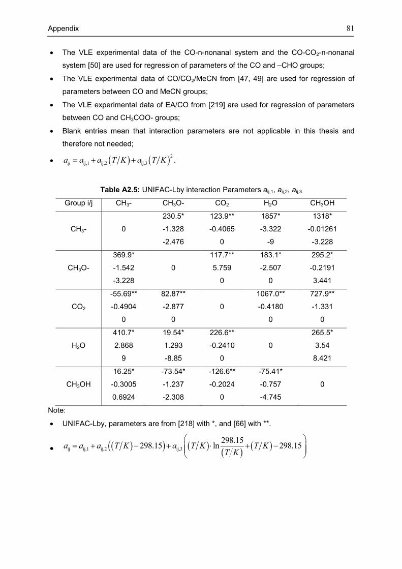
Appendix 81
• The VLE experimental data of the CO-n-nonanal system and the CO-CO2-n-nonanal
system [50] are used for regression of parameters of the CO and –CHO groups;
• The VLE experimental data of CO/CO2/MeCN from [47, 49] are used for regression of
parameters between CO and MeCN groups;
• The VLE experimental data of EA/CO from [219] are used for regression of parameters
between CO and CH3COO- groups;
• Blank entries mean that interaction parameters are not applicable in this thesis and
therefore not needed;
• ( ) ( )2
ij,1 ij,2 ij,3ija a a T K a T K= + + .
Table A2.5: UNIFAC-Lby interaction Parameters aij,1, aij,2, aij,3
Group i/j CH3- CH3O- CO2 H2O CH3OH
CH3- 0
230.5*
-1.328
-2.476
123.9**
-0.4065
0
1857*
-3.322
-9
1318*
-0.01261
-3.228
CH3O-
369.9*
-1.542
-3.228
0
117.7**
5.759
0
183.1*
-2.507
0
295.2*
-0.2191
3.441
CO2
-55.69**
-0.4904
0
82.87**
-2.877
0
0
1067.0**
-0.4180
0
727.9**
-1.331
0
H2O
410.7*
2.868
9
19.54*
1.293
-8.85
226.6**
-0.2410
0
0
265.5*
3.54
8.421
CH3OH
16.25*
-0.3005
0.6924
-73.54*
-1.237
-2.308
-126.6**
-0.2024
0
-75.41*
-0.757
-4.745
0
Note:
• UNIFAC-Lby, parameters are from [218] with *, and [66] with **.
• ( )( ) ( )( )
( )ij ij,1 ij,2 ij,3
298.15298.15 ln 298.15a a a T K a T K T K
T K
= + − + ⋅ + −
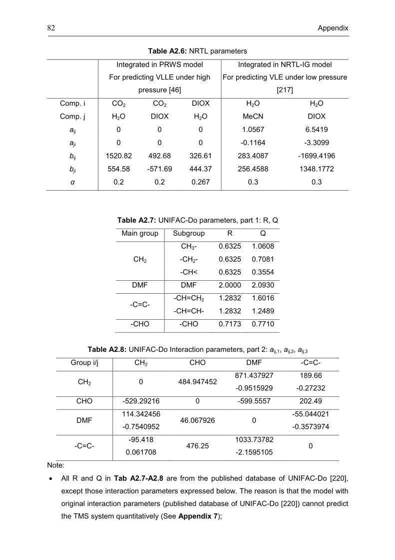
82 Appendix
Table A2.6: NRTL parameters
Integrated in PRWS model
For predicting VLLE under high
pressure [46]
Integrated in NRTL-IG model
For predicting VLE under low pressure
[217]
Comp. i CO2 CO2 DIOX H2O H2O
Comp. j H2O DIOX H2O MeCN DIOX
aij 0 0 0 1.0567 6.5419
aji 0 0 0 -0.1164 -3.3099
bij 1520.82 492.68 326.61 283.4087 -1699.4196
bji 554.58 -571.69 444.37 256.4588 1348.1772
α 0.2 0.2 0.267 0.3 0.3
Table A2.7: UNIFAC-Do parameters, part 1: R, Q
Main group Subgroup R Q
CH2
CH3- 0.6325 1.0608
-CH2- 0.6325 0.7081
-CH< 0.6325 0.3554
DMF DMF 2.0000 2.0930
-C=C- -CH=CH2 1.2832 1.6016
-CH=CH- 1.2832 1.2489
-CHO -CHO 0.7173 0.7710
Table A2.8: UNIFAC-Do Interaction parameters, part 2: aij,1, aij,2, aij,3
Group i/j CH2 CHO DMF -C=C-
CH2 0 484.947452 871.437927
-0.9515929
189.66
-0.27232
CHO -529.29216 0 -599.5557 202.49
DMF 114.342456
-0.7540952 46.067926 0
-55.044021
-0.3573974
-C=C- -95.418
0.061708 476.25
1033.73782
-2.1595105 0
Note:
• All R and Q in Tab A2.7-A2.8 are from the published database of UNIFAC-Do [220],
except those interaction parameters expressed below. The reason is that the model with
original interaction parameters (published database of UNIFAC-Do [220]) cannot predict
the TMS system quantitatively (See Appendix 7);
Appendix 83
• The interaction parameters of DMF/CH2 are regressed from binary LLE data [214] of
DMF/n-decane; the interaction parameters of DMF/-C=C- are regressed from binary LLE
data [214] of DMF/1-dodecene; the interaction parameters of CH2 and CHO, DMF and
CHO group are regressed using the ternary LLE experimental data of DMF/1-dodecanal/
n-decane [214]. The regression procedure using Aspen Properties (maximum likelihood
method) is the same as the reference [52];
• ( ) ( )2
ij,1 ij,2 ij,3ija a a T K a T K= + + .
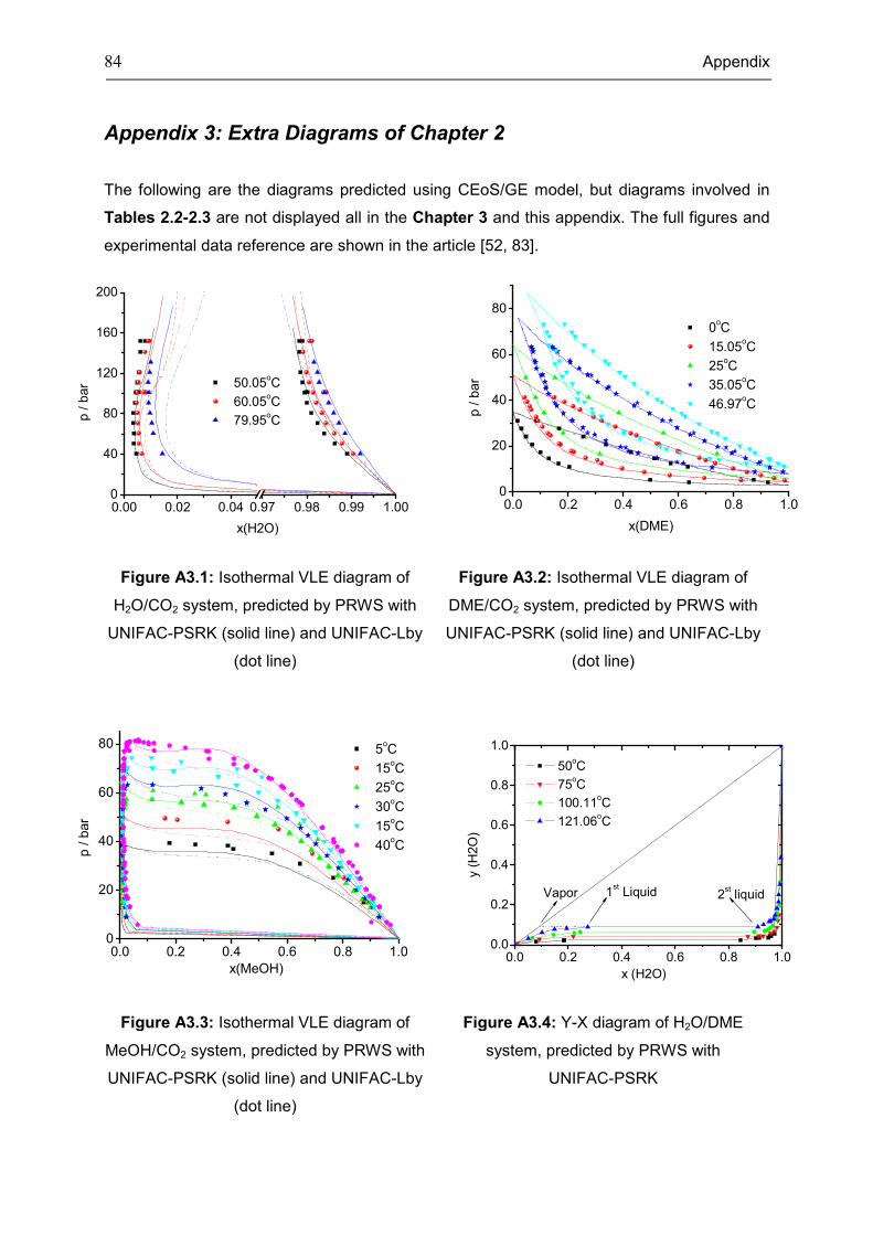
84 Appendix
Appendix 3: Extra Diagrams of Chapter 2
The following are the diagrams predicted using CEoS/GE model, but diagrams involved in
Tables 2.2-2.3 are not displayed all in the Chapter 3 and this appendix. The full figures and
experimental data reference are shown in the article [52, 83].
Figure A3.1: Isothermal VLE diagram of
H2O/CO2 system, predicted by PRWS with
UNIFAC-PSRK (solid line) and UNIFAC-Lby
(dot line)
Figure A3.2: Isothermal VLE diagram of
DME/CO2 system, predicted by PRWS with
UNIFAC-PSRK (solid line) and UNIFAC-Lby
(dot line)
Figure A3.3: Isothermal VLE diagram of
MeOH/CO2 system, predicted by PRWS with
UNIFAC-PSRK (solid line) and UNIFAC-Lby
(dot line)
Figure A3.4: Y-X diagram of H2O/DME
system, predicted by PRWS with
UNIFAC-PSRK
0.00 0.02 0.04 0.97 0.98 0.99 1.000
40
80
120
160
200
50.05oC
60.05oC
79.95oCp
/ b
ar
x(H2O)
0.0 0.2 0.4 0.6 0.8 1.00
20
40
60
80
0oC
15.05oC
25oC
35.05oC
46.97oC
p / b
ar
x(DME)
0.0 0.2 0.4 0.6 0.8 1.00
20
40
60
80 5oC
15oC
25oC
30oC
15oC
40oC
p /
bar
x(MeOH)0.0 0.2 0.4 0.6 0.8 1.0
0.0
0.2
0.4
0.6
0.8
1.0
1st Liquid 2
st liquid
y (
H2O
)
x (H2O)
50oC
75oC
100.11oC
121.06oC
Vapor
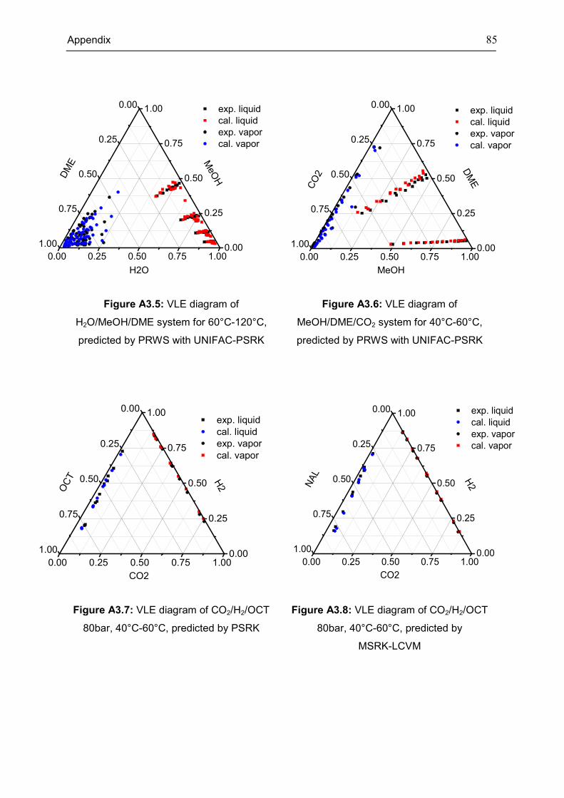
Appendix 85
Figure A3.5: VLE diagram of
H2O/MeOH/DME system for 60°C-120°C,
predicted by PRWS with UNIFAC-PSRK
Figure A3.6: VLE diagram of
MeOH/DME/CO2 system for 40°C-60°C,
predicted by PRWS with UNIFAC-PSRK
Figure A3.7: VLE diagram of CO2/H2/OCT
80bar, 40°C-60°C, predicted by PSRK
Figure A3.8: VLE diagram of CO2/H2/OCT
80bar, 40°C-60°C, predicted by
MSRK-LCVM
0.00 0.25 0.50 0.75 1.000.00
0.25
0.50
0.75
1.000.00
0.25
0.50
0.75
1.00
exp. liquid
cal. liquid
exp. vapor
cal. vapor
MeO
HDM
E
H2O
0.00 0.25 0.50 0.75 1.000.00
0.25
0.50
0.75
1.000.00
0.25
0.50
0.75
1.00
exp. liquid
cal. liquid
exp. vapor
cal. vapor
DM
E
CO
2
MeOH
0.00 0.25 0.50 0.75 1.000.00
0.25
0.50
0.75
1.000.00
0.25
0.50
0.75
1.00
exp. liquid
cal. liquid
exp. vapor
cal. vapor
H2
OC
T
CO2
0.00 0.25 0.50 0.75 1.000.00
0.25
0.50
0.75
1.000.00
0.25
0.50
0.75
1.00
exp. liquid
cal. liquid
exp. vapor
cal. vapor
H2N
AL
CO2
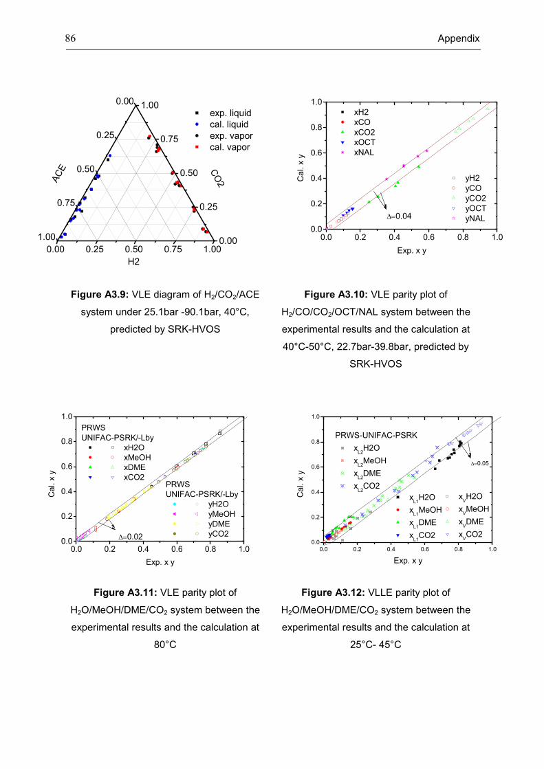
86 Appendix
Figure A3.9: VLE diagram of H2/CO2/ACE
system under 25.1bar -90.1bar, 40°C,
predicted by SRK-HVOS
Figure A3.10: VLE parity plot of
H2/CO/CO2/OCT/NAL system between the
experimental results and the calculation at
40°C-50°C, 22.7bar-39.8bar, predicted by
SRK-HVOS
Figure A3.11: VLE parity plot of
H2O/MeOH/DME/CO2 system between the
experimental results and the calculation at
80°C
Figure A3.12: VLLE parity plot of
H2O/MeOH/DME/CO2 system between the
experimental results and the calculation at
25°C- 45°C
0.00 0.25 0.50 0.75 1.000.00
0.25
0.50
0.75
1.000.00
0.25
0.50
0.75
1.00
exp. liquid
cal. liquid
exp. vapor
cal. vapor
CO
2AC
E
H2
0.0 0.2 0.4 0.6 0.8 1.00.0
0.2
0.4
0.6
0.8
1.0
Ca
l. x
y
Exp. x y
xH2
xCO
xCO2
xOCT
xNAL
yH2
yCO
yCO2
yOCT
yNAL∆=0.04
0.0 0.2 0.4 0.6 0.8 1.00.0
0.2
0.4
0.6
0.8
1.0
PRWS
UNIFAC-PSRK/-Lby
yH2O
yMeOH
yDME
yCO2∆=0.02
Cal. x
y
Exp. x y
PRWS
UNIFAC-PSRK/-Lby
xH2O
xMeOH
xDME
xCO2
0.0 0.2 0.4 0.6 0.8 1.0
0.0
0.2
0.4
0.6
0.8
1.0
∆=0.05
xL1
H2O
xL1
MeOH
xL1
DME
xL1
CO2
xVH2O
xVMeOH
xVDME
xVCO2
Cal. x
y
Exp. x y
xL2
H2O
xL2
MeOH
xL2
DME
xL2
CO2
PRWS-UNIFAC-PSRK
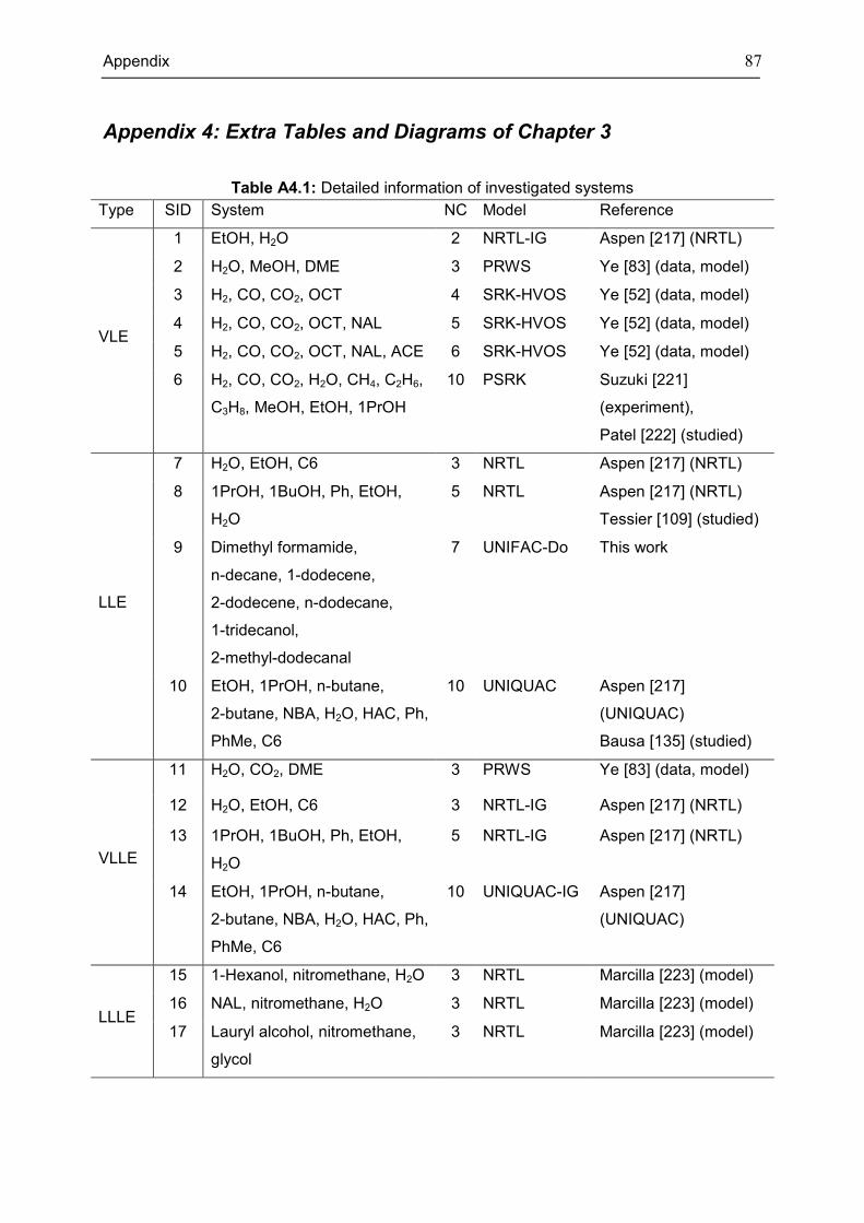
Appendix 87
Appendix 4: Extra Tables and Diagrams of Chapter 3
Table A4.1: Detailed information of investigated systems
Type SID System NC Model Reference
VLE
1 EtOH, H2O 2 NRTL-IG Aspen [217] (NRTL)
2 H2O, MeOH, DME 3 PRWS Ye [83] (data, model)
3 H2, CO, CO2, OCT 4 SRK-HVOS Ye [52] (data, model)
4 H2, CO, CO2, OCT, NAL 5 SRK-HVOS Ye [52] (data, model)
5 H2, CO, CO2, OCT, NAL, ACE 6 SRK-HVOS Ye [52] (data, model)
6 H2, CO, CO2, H2O, CH4, C2H6,
C3H8, MeOH, EtOH, 1PrOH
10 PSRK Suzuki [221]
(experiment),
Patel [222] (studied)
LLE
7 H2O, EtOH, C6 3 NRTL Aspen [217] (NRTL)
8 1PrOH, 1BuOH, Ph, EtOH,
H2O
5 NRTL Aspen [217] (NRTL)
Tessier [109] (studied)
9 Dimethyl formamide,
n-decane, 1-dodecene,
2-dodecene, n-dodecane,
1-tridecanol,
2-methyl-dodecanal
7 UNIFAC-Do This work
10 EtOH, 1PrOH, n-butane,
2-butane, NBA, H2O, HAC, Ph,
PhMe, C6
10 UNIQUAC Aspen [217]
(UNIQUAC)
Bausa [135] (studied)
VLLE
11 H2O, CO2, DME 3 PRWS Ye [83] (data, model)
12 H2O, EtOH, C6 3 NRTL-IG Aspen [217] (NRTL)
13 1PrOH, 1BuOH, Ph, EtOH,
H2O
5 NRTL-IG Aspen [217] (NRTL)
14 EtOH, 1PrOH, n-butane,
2-butane, NBA, H2O, HAC, Ph,
PhMe, C6
10 UNIQUAC-IG Aspen [217]
(UNIQUAC)
LLLE
15 1-Hexanol, nitromethane, H2O 3 NRTL Marcilla [223] (model)
16 NAL, nitromethane, H2O 3 NRTL Marcilla [223] (model)
17 Lauryl alcohol, nitromethane,
glycol
3 NRTL Marcilla [223] (model)
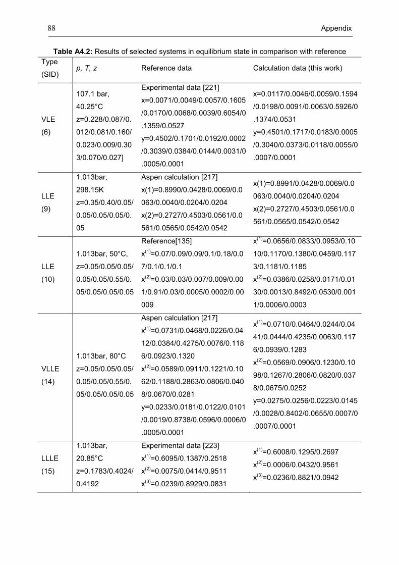
88 Appendix
Table A4.2: Results of selected systems in equilibrium state in comparison with reference
Type
(SID) p, T, z Reference data Calculation data (this work)
VLE
(6)
107.1 bar,
40.25°C
z=0.228/0.087/0.
012/0.081/0.160/
0.023/0.009/0.30
3/0.070/0.027]
Experimental data [221]
x=0.0071/0.0049/0.0057/0.1605
/0.0170/0.0068/0.0039/0.6054/0
.1359/0.0527
y=0.4502/0.1701/0.0192/0.0002
/0.3039/0.0384/0.0144/0.0031/0
.0005/0.0001
x=0.0117/0.0046/0.0059/0.1594
/0.0198/0.0091/0.0063/0.5926/0
.1374/0.0531
y=0.4501/0.1717/0.0183/0.0005
/0.3040/0.0373/0.0118/0.0055/0
.0007/0.0001
LLE
(9)
1.013bar,
298.15K
z=0.35/0.40/0.05/
0.05/0.05/0.05/0.
05
Aspen calculation [217]
x(1)=0.8990/0.0428/0.0069/0.0
063/0.0040/0.0204/0.0204
x(2)=0.2727/0.4503/0.0561/0.0
561/0.0565/0.0542/0.0542
x(1)=0.8991/0.0428/0.0069/0.0
063/0.0040/0.0204/0.0204
x(2)=0.2727/0.4503/0.0561/0.0
561/0.0565/0.0542/0.0542
LLE
(10)
1.013bar, 50°C,
z=0.05/0.05/0.05/
0.05/0.05/0.55/0.
05/0.05/0.05/0.05
Reference[135]
x(1)=0.07/0.09/0.09/0.1/0.18/0.0
7/0.1/0.1/0.1
x(2)=0.03/0.03/0.007/0.009/0.00
1/0.91/0.03/0.0005/0.0002/0.00
009
x(1)=0.0656/0.0833/0.0953/0.10
10/0.1170/0.1380/0.0459/0.117
3/0.1181/0.1185
x(2)=0.0386/0.0258/0.0171/0.01
30/0.0013/0.8492/0.0530/0.001
1/0.0006/0.0003
VLLE
(14)
1.013bar, 80°C
z=0.05/0.05/0.05/
0.05/0.05/0.55/0.
05/0.05/0.05/0.05
Aspen calculation [217]
x(1)=0.0731/0.0468/0.0226/0.04
12/0.0384/0.4275/0.0076/0.118
6/0.0923/0.1320
x(2)=0.0589/0.0911/0.1221/0.10
62/0.1188/0.2863/0.0806/0.040
8/0.0670/0.0281
y=0.0233/0.0181/0.0122/0.0101
/0.0019/0.8738/0.0596/0.0006/0
.0005/0.0001
x(1)=0.0710/0.0464/0.0244/0.04
41/0.0444/0.4235/0.0063/0.117
6/0.0939/0.1283
x(2)=0.0569/0.0906/0.1230/0.10
98/0.1267/0.2806/0.0820/0.037
8/0.0675/0.0252
y=0.0275/0.0256/0.0223/0.0145
/0.0028/0.8402/0.0655/0.0007/0
.0007/0.0001
LLLE
(15)
1.013bar,
20.85°C
z=0.1783/0.4024/
0.4192
Experimental data [223]
x(1)=0.6095/0.1387/0.2518
x(2)=0.0075/0.0414/0.9511
x(3)=0.0239/0.8929/0.0831
x(1)=0.6008/0.1295/0.2697
x(2)=0.0006/0.0432/0.9561
x(3)=0.0236/0.8821/0.0942
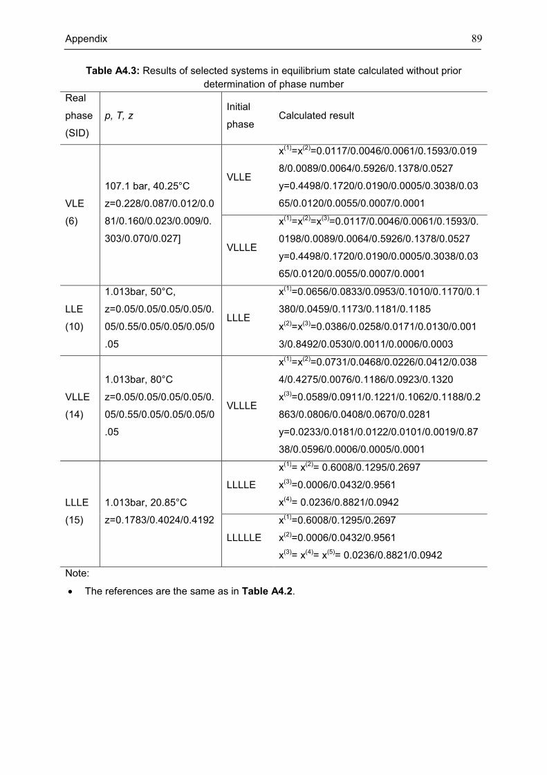
Appendix 89
Table A4.3: Results of selected systems in equilibrium state calculated without prior
determination of phase number
Real
phase
(SID)
p, T, z Initial
phase Calculated result
VLE
(6)
107.1 bar, 40.25°C
z=0.228/0.087/0.012/0.0
81/0.160/0.023/0.009/0.
303/0.070/0.027]
VLLE
x(1)=x(2)=0.0117/0.0046/0.0061/0.1593/0.019
8/0.0089/0.0064/0.5926/0.1378/0.0527
y=0.4498/0.1720/0.0190/0.0005/0.3038/0.03
65/0.0120/0.0055/0.0007/0.0001
VLLLE
x(1)=x(2)=x(3)=0.0117/0.0046/0.0061/0.1593/0.
0198/0.0089/0.0064/0.5926/0.1378/0.0527
y=0.4498/0.1720/0.0190/0.0005/0.3038/0.03
65/0.0120/0.0055/0.0007/0.0001
LLE
(10)
1.013bar, 50°C,
z=0.05/0.05/0.05/0.05/0.
05/0.55/0.05/0.05/0.05/0
.05
LLLE
x(1)=0.0656/0.0833/0.0953/0.1010/0.1170/0.1
380/0.0459/0.1173/0.1181/0.1185
x(2)=x(3)=0.0386/0.0258/0.0171/0.0130/0.001
3/0.8492/0.0530/0.0011/0.0006/0.0003
VLLE
(14)
1.013bar, 80°C
z=0.05/0.05/0.05/0.05/0.
05/0.55/0.05/0.05/0.05/0
.05
VLLLE
x(1)=x(2)=0.0731/0.0468/0.0226/0.0412/0.038
4/0.4275/0.0076/0.1186/0.0923/0.1320
x(3)=0.0589/0.0911/0.1221/0.1062/0.1188/0.2
863/0.0806/0.0408/0.0670/0.0281
y=0.0233/0.0181/0.0122/0.0101/0.0019/0.87
38/0.0596/0.0006/0.0005/0.0001
LLLE
(15)
1.013bar, 20.85°C
z=0.1783/0.4024/0.4192
LLLLE
x(1)= x(2)= 0.6008/0.1295/0.2697
x(3)=0.0006/0.0432/0.9561
x(4)= 0.0236/0.8821/0.0942
LLLLLE
x(1)=0.6008/0.1295/0.2697
x(2)=0.0006/0.0432/0.9561
x(3)= x(4)= x(5)= 0.0236/0.8821/0.0942
Note:
• The references are the same as in Table A4.2.
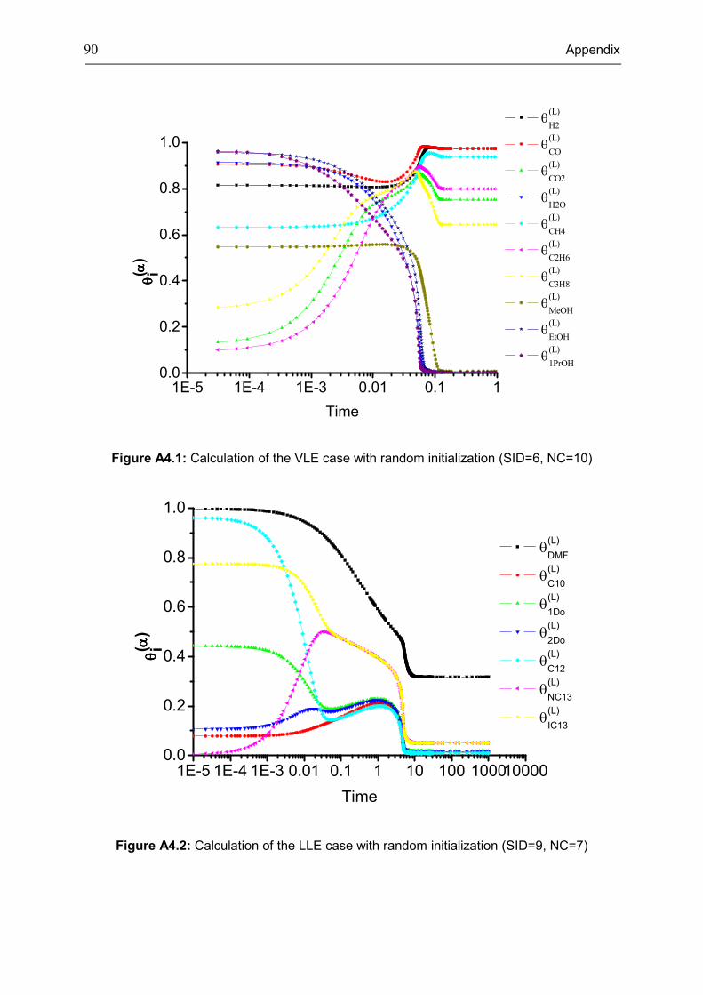
90 Appendix
Figure A4.1: Calculation of the VLE case with random initialization (SID=6, NC=10)
Figure A4.2: Calculation of the LLE case with random initialization (SID=9, NC=7)
1E-5 1E-4 1E-3 0.01 0.1 10.0
0.2
0.4
0.6
0.8
1.0θθ θθ( αα αα
)i
Time
θ(L)
H2
θ(L)
CO
θ(L)
CO2
θ(L)
H2O
θ(L)
CH4
θ(L)
C2H6
θ(L)
C3H8
θ(L)
MeOH
θ(L)
EtOH
θ(L)
1PrOH
1E-5 1E-4 1E-3 0.01 0.1 1 10 100 1000100000.0
0.2
0.4
0.6
0.8
1.0
θ(L)
DMF
θ(L)
C10
θ(L)
1Do
θ(L)
2Do
θ(L)
C12
θ(L)
NC13
θ(L)
IC13
θθ θθ( αα αα)
i
Time
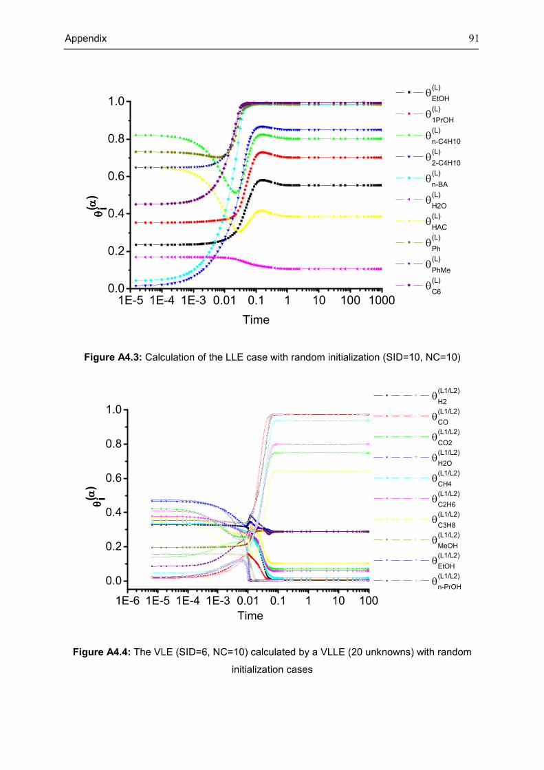
Appendix 91
Figure A4.3: Calculation of the LLE case with random initialization (SID=10, NC=10)
Figure A4.4: The VLE (SID=6, NC=10) calculated by a VLLE (20 unknowns) with random
initialization cases
1E-5 1E-4 1E-3 0.01 0.1 1 10 100 10000.0
0.2
0.4
0.6
0.8
1.0θθ θθ( αα αα
)i
Time
θ(L)
EtOH
θ(L)
1PrOH
θ(L)
n-C4H10
θ(L)
2-C4H10
θ(L)
n-BA
θ(L)
H2O
θ(L)
HAC
θ(L)
Ph
θ(L)
PhMe
θ(L)
C6
1E-6 1E-5 1E-4 1E-3 0.01 0.1 1 10 100
0.0
0.2
0.4
0.6
0.8
1.0
θ(L1/L2)
H2
θ(L1/L2)
CO
θ(L1/L2)
CO2
θ(L1/L2)
H2O
θ(L1/L2)
CH4
θ(L1/L2)
C2H6
θ(L1/L2)
C3H8
θ(L1/L2)
MeOH
θ(L1/L2)
EtOH
θ(L1/L2)
n-PrOH
Time
θθ θθ( αα αα)
i
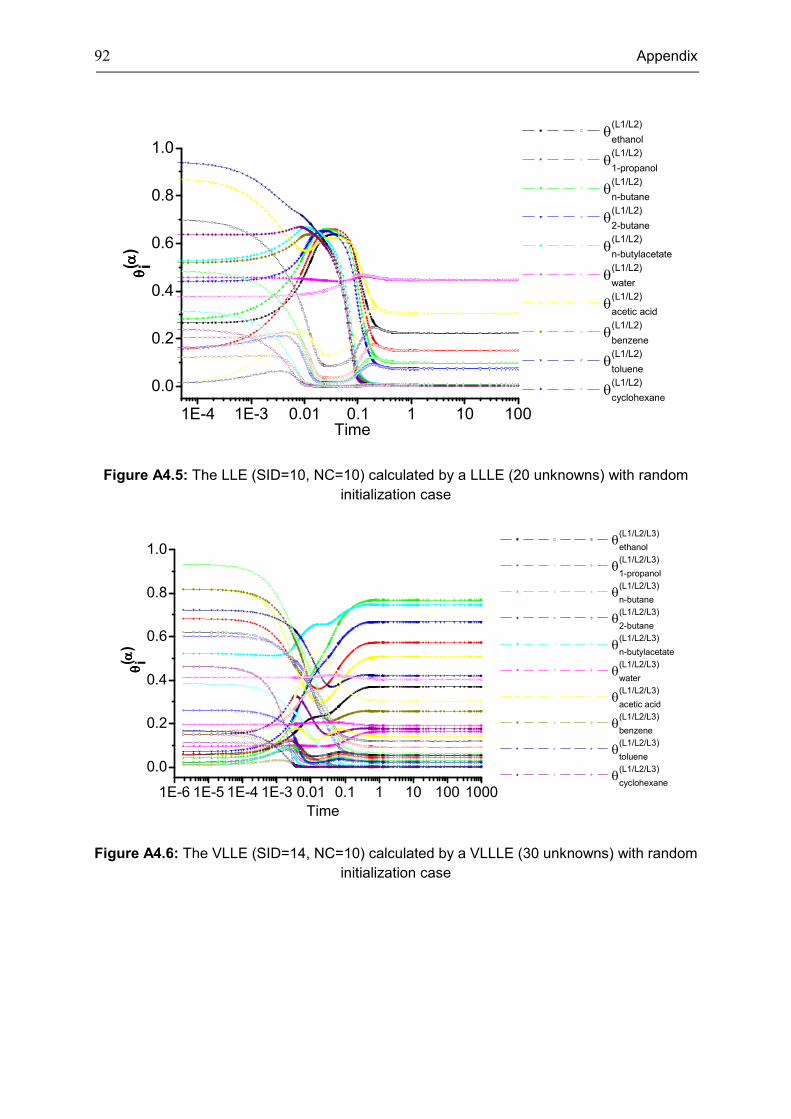
92 Appendix
Figure A4.5: The LLE (SID=10, NC=10) calculated by a LLLE (20 unknowns) with random
initialization case
Figure A4.6: The VLLE (SID=14, NC=10) calculated by a VLLLE (30 unknowns) with random
initialization case
1E-4 1E-3 0.01 0.1 1 10 100
0.0
0.2
0.4
0.6
0.8
1.0 θ
(L1/L2)
ethanol
θ(L1/L2)
1-propanol
θ(L1/L2)
n-butane
θ(L1/L2)
2-butane
θ(L1/L2)
n-butylacetate
θ(L1/L2)
water
θ(L1/L2)
acetic acid
θ(L1/L2)
benzene
θ(L1/L2)
toluene
θ(L1/L2)
cyclohexane
Time
θθ θθ( αα αα)
i
1E-6 1E-5 1E-4 1E-3 0.01 0.1 1 10 100 1000
0.0
0.2
0.4
0.6
0.8
1.0 θ
(L1/L2/L3)
ethanol
θ(L1/L2/L3)
1-propanol
θ(L1/L2/L3)
n-butane
θ(L1/L2/L3)
2-butane
θ(L1/L2/L3)
n-butylacetate
θ(L1/L2/L3)
water
θ(L1/L2/L3)
acetic acid
θ(L1/L2/L3)
benzene
θ(L1/L2/L3)
toluene
θ(L1/L2/L3)
cyclohexane
Time
θθ θθ( αα αα)
i
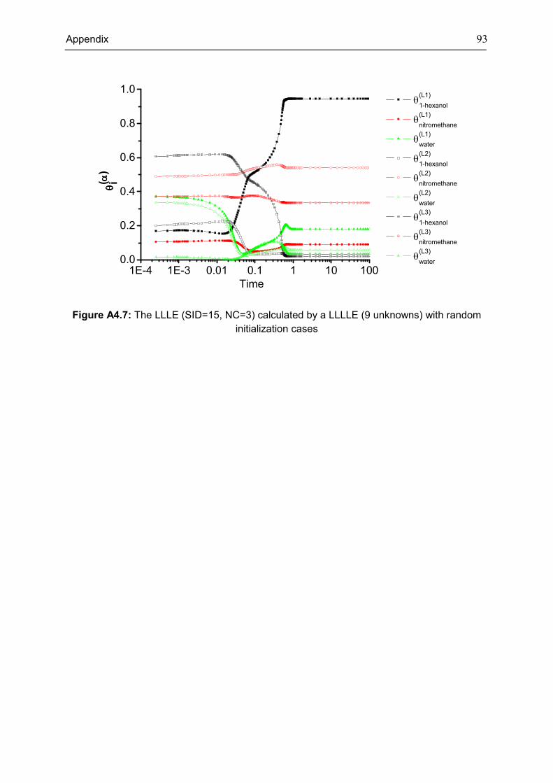
Appendix 93
Figure A4.7: The LLLE (SID=15, NC=3) calculated by a LLLLE (9 unknowns) with random
initialization cases
1E-4 1E-3 0.01 0.1 1 10 1000.0
0.2
0.4
0.6
0.8
1.0 θ
(L1)
1-hexanol
θ(L1)
nitromethane
θ(L1)
water
θ(L2)
1-hexanol
θ(L2)
nitromethane
θ(L2)
water
θ(L3)
1-hexanol
θ(L3)
nitromethane
θ(L3)
water
θθ θθ( αα αα)
i
Time
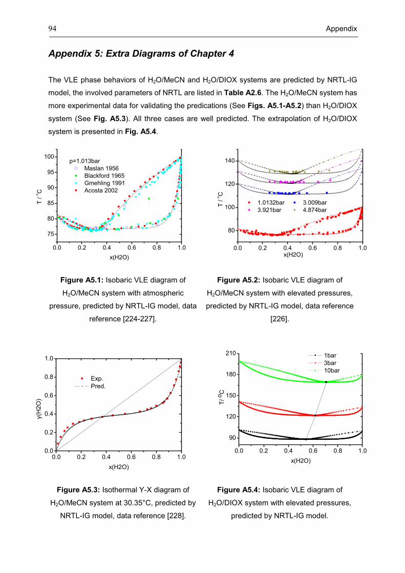
94 Appendix
Appendix 5: Extra Diagrams of Chapter 4
The VLE phase behaviors of H2O/MeCN and H2O/DIOX systems are predicted by NRTL-IG
model, the involved parameters of NRTL are listed in Table A2.6. The H2O/MeCN system has
more experimental data for validating the predications (See Figs. A5.1-A5.2) than H2O/DIOX
system (See Fig. A5.3). All three cases are well predicted. The extrapolation of H2O/DIOX
system is presented in Fig. A5.4.
Figure A5.1: Isobaric VLE diagram of
H2O/MeCN system with atmospheric
pressure, predicted by NRTL-IG model, data
reference [224-227].
Figure A5.2: Isobaric VLE diagram of
H2O/MeCN system with elevated pressures,
predicted by NRTL-IG model, data reference
[226].
Figure A5.3: Isothermal Y-X diagram of
H2O/MeCN system at 30.35°C, predicted by
NRTL-IG model, data reference [228].
Figure A5.4: Isobaric VLE diagram of
H2O/DIOX system with elevated pressures,
predicted by NRTL-IG model.
0.0 0.2 0.4 0.6 0.8 1.0
75
80
85
90
95
100
T /
oC
x(H2O)
p=1.013bar
Maslan 1956
Blackford 1965
Gmehling 1991
Acosta 2002
0.0 0.2 0.4 0.6 0.8 1.0
80
100
120
140
1.0132bar 3.009bar
3.921bar 4.874bar
T / o
C
x(H2O)
0.0 0.2 0.4 0.6 0.8 1.00.0
0.2
0.4
0.6
0.8
1.0
y(H
2O
)
x(H2O)
Exp.
Pred.
0.0 0.2 0.4 0.6 0.8 1.0
90
120
150
180
210
T/
oC
x(H2O)
1bar
3bar
10bar
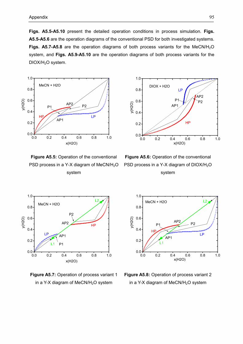
Appendix 95
Figs. A5.5-A5.10 present the detailed operation conditions in process simulation. Figs.
A5.5-A5.6 are the operation diagrams of the conventional PSD for both investigated systems.
Figs. A5.7-A5.8 are the operation diagrams of both process variants for the MeCN/H2O
system, and Figs. A5.9-A5.10 are the operation diagrams of both process variants for the
DIOX/H2O system.
Figure A5.5: Operation of the conventional
PSD process in a Y-X diagram of MeCN/H2O
system
Figure A5.6: Operation of the conventional
PSD process in a Y-X diagram of DIOX/H2O
system
Figure A5.7: Operation of process variant 1
in a Y-X diagram of MeCN/H2O system
Figure A5.8: Operation of process variant 2
in a Y-X diagram of MeCN/H2O system
0.0 0.2 0.4 0.6 0.8 1.00.0
0.2
0.4
0.6
0.8
1.0
MeCN + H2O
P2P1
LPHPAP1
y(H
2O
)
x(H2O)
AP2
0.0 0.2 0.4 0.6 0.8 1.00.0
0.2
0.4
0.6
0.8
1.0
DIOX + H2O
AP2
AP1P2
P1
LP
HP
y(H
2O
)
x(H2O)
0.0 0.2 0.4 0.6 0.8 1.00.0
0.2
0.4
0.6
0.8
1.0
MeCN + H2OL2
P1
P2
L1
LP
HP
AP1
y(H
2O
)
x(H2O)
AP2
0.0 0.2 0.4 0.6 0.8 1.00.0
0.2
0.4
0.6
0.8
1.0
MeCN + H2O
L1
L2
P2P1
LPHP
AP1
y(H
2O
)
x(H2O)
AP2
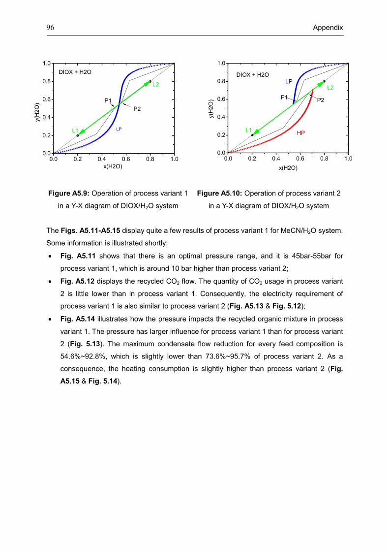
96 Appendix
Figure A5.9: Operation of process variant 1
in a Y-X diagram of DIOX/H2O system
Figure A5.10: Operation of process variant 2
in a Y-X diagram of DIOX/H2O system
The Figs. A5.11-A5.15 display quite a few results of process variant 1 for MeCN/H2O system.
Some information is illustrated shortly:
• Fig. A5.11 shows that there is an optimal pressure range, and it is 45bar-55bar for
process variant 1, which is around 10 bar higher than process variant 2;
• Fig. A5.12 displays the recycled CO2 flow. The quantity of CO2 usage in process variant
2 is little lower than in process variant 1. Consequently, the electricity requirement of
process variant 1 is also similar to process variant 2 (Fig. A5.13 & Fig. 5.12);
• Fig. A5.14 illustrates how the pressure impacts the recycled organic mixture in process
variant 1. The pressure has larger influence for process variant 1 than for process variant
2 (Fig. 5.13). The maximum condensate flow reduction for every feed composition is
54.6%~92.8%, which is slightly lower than 73.6%~95.7% of process variant 2. As a
consequence, the heating consumption is slightly higher than process variant 2 (Fig.
A5.15 & Fig. 5.14).
0.0 0.2 0.4 0.6 0.8 1.00.0
0.2
0.4
0.6
0.8
1.0
DIOX + H2O
P2
P1
L2
L1
y(H
2O
)
x(H2O)
LP
0.0 0.2 0.4 0.6 0.8 1.00.0
0.2
0.4
0.6
0.8
1.0
DIOX + H2O
P2P1
L2
L1
LP
HP
y(H
2O
)
x(H2O)
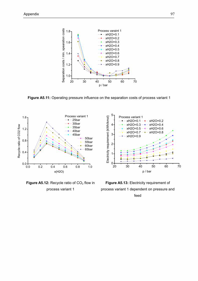
Appendix 97
Figure A5.11: Operating pressure influence on the separation costs of process variant 1
Figure A5.12: Recycle ratio of CO2 flow in
process variant 1
Figure A5.13: Electricity requirement of
process variant 1 dependent on pressure and
feed
20 30 40 50 60 70
1.0
1.2
1.4
1.6
1.8
p / bar
Sep
ara
tion
co
sts
/ m
in. spe
ara
tion
costs Process varaint 1
xH2O=0.1
xH2O=0.2
xH2O=0.3
xH2O=0.4
xH2O=0.5
xH2O=0.6
xH2O=0.7
xH2O=0.8
xH2O=0.9
0.0 0.2 0.4 0.6 0.8 1.00.0
0.4
0.8
1.2
1.6
50bar
55bar
60bar
65bar
Process variant 1
25bar
30bar
35bar
40bar
45bar
Recycle
ratio
of
CO
2 f
low
x(H2O)
20 30 40 50 60 700
1
2
3
4
5Process variant 1
xH2O=0.1 xH2O=0.2
xH2O=0.3 xH2O=0.4
xH2O=0.5 xH2O=0.6
xH2O=0.7 xH2O=0.8
xH2O=0.9
Ele
ctr
icity r
equir
em
ent
(kW
h/k
mol)
p / bar
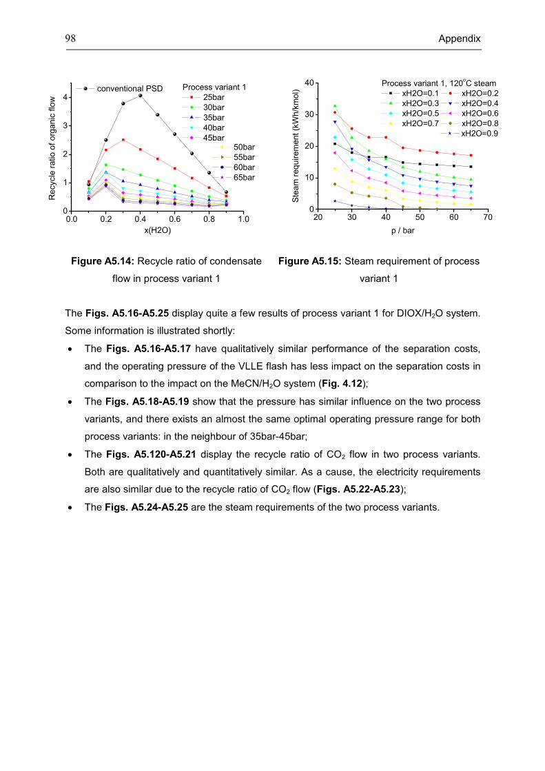
98 Appendix
Figure A5.14: Recycle ratio of condensate
flow in process variant 1
Figure A5.15: Steam requirement of process
variant 1
The Figs. A5.16-A5.25 display quite a few results of process variant 1 for DIOX/H2O system.
Some information is illustrated shortly:
• The Figs. A5.16-A5.17 have qualitatively similar performance of the separation costs,
and the operating pressure of the VLLE flash has less impact on the separation costs in
comparison to the impact on the MeCN/H2O system (Fig. 4.12);
• The Figs. A5.18-A5.19 show that the pressure has similar influence on the two process
variants, and there exists an almost the same optimal operating pressure range for both
process variants: in the neighbour of 35bar-45bar;
• The Figs. A5.120-A5.21 display the recycle ratio of CO2 flow in two process variants.
Both are qualitatively and quantitatively similar. As a cause, the electricity requirements
are also similar due to the recycle ratio of CO2 flow (Figs. A5.22-A5.23);
• The Figs. A5.24-A5.25 are the steam requirements of the two process variants.
0.0 0.2 0.4 0.6 0.8 1.00
1
2
3
4
50bar
55bar
60bar
65bar
Process variant 1
25bar
30bar
35bar
40bar
45bar
conventional PSD
Re
cycle
ratio
of
org
an
ic f
low
x(H2O)
20 30 40 50 60 700
10
20
30
40
Ste
am
req
uire
ment
(kW
h/k
mol)
p / bar
Process variant 1, 120oC steam
xH2O=0.1 xH2O=0.2
xH2O=0.3 xH2O=0.4
xH2O=0.5 xH2O=0.6
xH2O=0.7 xH2O=0.8
xH2O=0.9
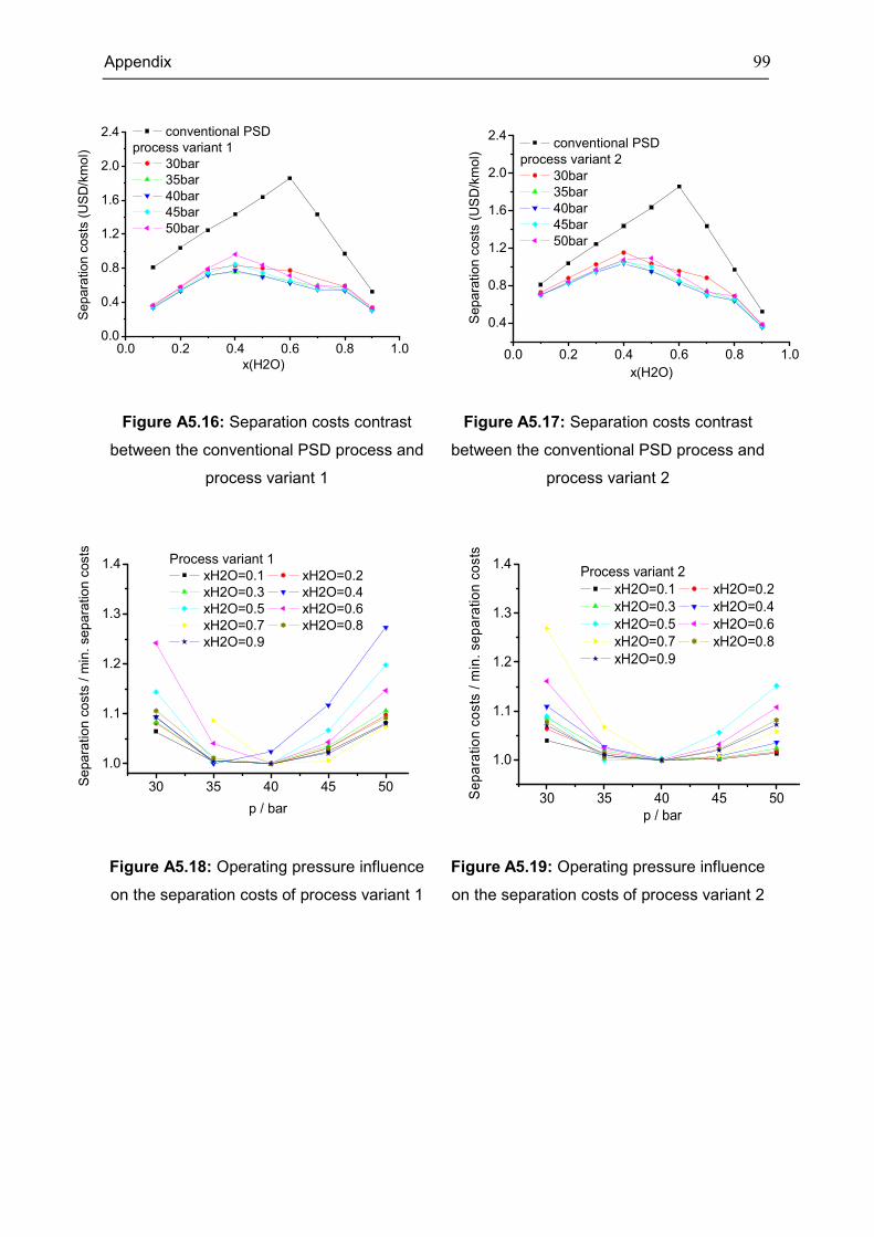
Appendix 99
Figure A5.16: Separation costs contrast
between the conventional PSD process and
process variant 1
Figure A5.17: Separation costs contrast
between the conventional PSD process and
process variant 2
Figure A5.18: Operating pressure influence
on the separation costs of process variant 1
Figure A5.19: Operating pressure influence
on the separation costs of process variant 2
0.0 0.2 0.4 0.6 0.8 1.00.0
0.4
0.8
1.2
1.6
2.0
2.4
x(H2O)
Sep
ara
tio
n c
osts
(U
SD
/km
ol)
conventional PSD
process variant 1
30bar
35bar
40bar
45bar
50bar
0.0 0.2 0.4 0.6 0.8 1.0
0.4
0.8
1.2
1.6
2.0
2.4
Separa
tion c
osts
(U
SD
/km
ol)
x(H2O)
conventional PSD
process variant 2
30bar
35bar
40bar
45bar
50bar
30 35 40 45 50
1.0
1.1
1.2
1.3
1.4
Se
pa
ratio
n c
osts
/ m
in.
se
pa
ratio
n c
osts
p / bar
Process variant 1
xH2O=0.1 xH2O=0.2
xH2O=0.3 xH2O=0.4
xH2O=0.5 xH2O=0.6
xH2O=0.7 xH2O=0.8
xH2O=0.9
30 35 40 45 50
1.0
1.1
1.2
1.3
1.4Process variant 2
xH2O=0.1 xH2O=0.2
xH2O=0.3 xH2O=0.4
xH2O=0.5 xH2O=0.6
xH2O=0.7 xH2O=0.8
xH2O=0.9
Se
pa
ratio
n c
osts
/ m
in.
se
pa
ratio
n c
osts
p / bar
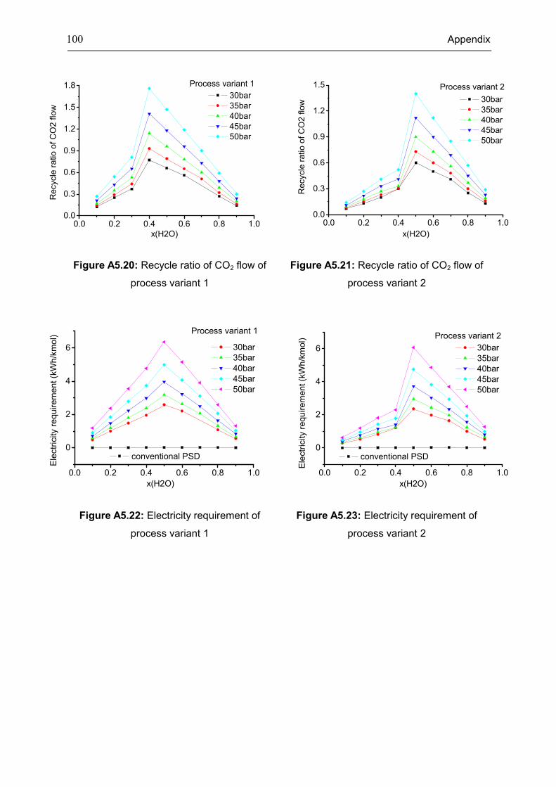
100 Appendix
Figure A5.20: Recycle ratio of CO2 flow of
process variant 1
Figure A5.21: Recycle ratio of CO2 flow of
process variant 2
Figure A5.22: Electricity requirement of
process variant 1
Figure A5.23: Electricity requirement of
process variant 2
0.0 0.2 0.4 0.6 0.8 1.00.0
0.3
0.6
0.9
1.2
1.5
1.8
30bar
35bar
40bar
45bar
50bar
Recycle
ra
tio
of C
O2
flo
w
x(H2O)
Process variant 1
0.0 0.2 0.4 0.6 0.8 1.00.0
0.3
0.6
0.9
1.2
1.5
30bar
35bar
40bar
45bar
50bar
Process variant 2
Recycle
ratio o
f C
O2
flo
w
x(H2O)
0.0 0.2 0.4 0.6 0.8 1.0
0
2
4
6
Process variant 1
30bar
35bar
40bar
45bar
50bar
Ele
ctr
icity r
eq
uir
em
en
t (k
Wh
/km
ol)
x(H2O)
conventional PSD
0.0 0.2 0.4 0.6 0.8 1.0
0
2
4
6 30bar
35bar
40bar
45bar
50bar
Process variant 2
Ele
ctr
icity r
equ
ire
me
nt (k
Wh
/km
ol)
x(H2O)
conventional PSD
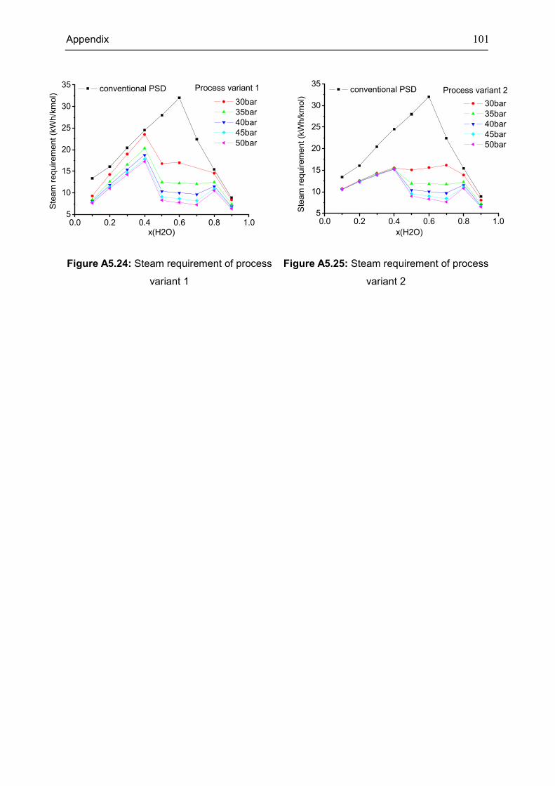
Appendix 101
Figure A5.24: Steam requirement of process
variant 1
Figure A5.25: Steam requirement of process
variant 2
0.0 0.2 0.4 0.6 0.8 1.05
10
15
20
25
30
35
30bar
35bar
40bar
45bar
50bar
Process variant 1
Ste
am
req
uir
em
en
t (k
Wh
/km
ol)
x(H2O)
conventional PSD
0.0 0.2 0.4 0.6 0.8 1.05
10
15
20
25
30
35
30bar
35bar
40bar
45bar
50bar
Process variant 2
Ste
am
req
uir
em
ent
(kW
h/k
mol)
x(H2O)
conventional PSD
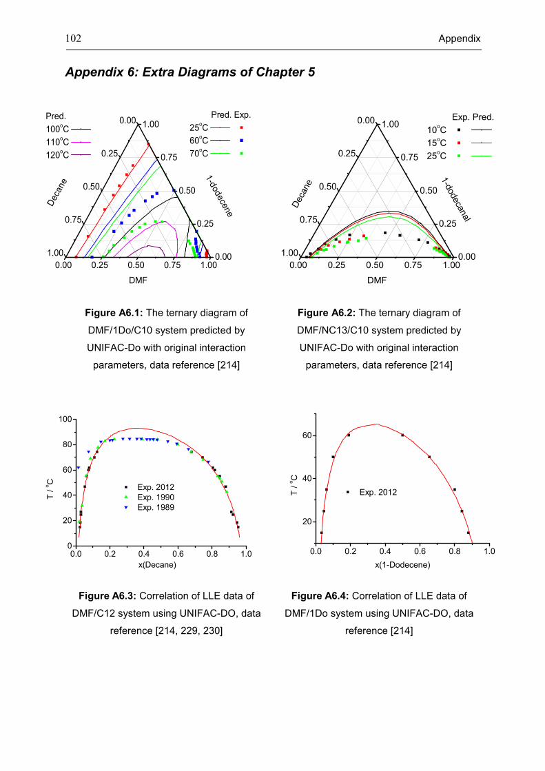
102 Appendix
Appendix 6: Extra Diagrams of Chapter 5
Figure A6.1: The ternary diagram of
DMF/1Do/C10 system predicted by
UNIFAC-Do with original interaction
parameters, data reference [214]
Figure A6.2: The ternary diagram of
DMF/NC13/C10 system predicted by
UNIFAC-Do with original interaction
parameters, data reference [214]
Figure A6.3: Correlation of LLE data of
DMF/C12 system using UNIFAC-DO, data
reference [214, 229, 230]
Figure A6.4: Correlation of LLE data of
DMF/1Do system using UNIFAC-DO, data
reference [214]
0.00 0.25 0.50 0.75 1.000.00
0.25
0.50
0.75
1.000.00
0.25
0.50
0.75
1.00
Pred.
100oC
110oC
120oC
1-d
odece
ne
Pred. Exp.
25oC
60oC
70oC
Deca
ne
DMF
0.00 0.25 0.50 0.75 1.000.00
0.25
0.50
0.75
1.000.00
0.25
0.50
0.75
1.00
1-d
odeca
nal
Exp. Pred.
10oC
15oC
25oC
Deca
ne
DMF
0.0 0.2 0.4 0.6 0.8 1.00
20
40
60
80
100
Exp. 2012
Exp. 1990
Exp. 1989
T /
oC
x(Decane)
0.0 0.2 0.4 0.6 0.8 1.0
20
40
60
T / o
C
x(1-Dodecene)
Exp. 2012
Bibliography 1. National Emissions Inventory (NEI) Air Pollutant Emissions Trends Data,
http://www.epa.gov/ttn/chief/trends/index.html. 2012. 2. Jones, A.P., Indoor air quality and health. Atmospheric Environment, 1999. 33(28):
4535-4564. 3. Anastas, P.T. and J.B. Zimmerman, Design through the 12 principles of green
engineering. Environmental Science & Technology, 2003. 37(5): 94-101. 4. Molina, M.J. and L.T. Molina, Megacities and atmospheric pollution. Journal of the Air
& Waste Management Association, 2004. 54(6): 644-680. 5. Jessop, P.G. and B. Subramaniam, Gas-expanded liquids. Chemical Reviews, 2007.
107(6): 2666-2694. 6. DeSimone, J.M., Practical approaches to green solvents. Science, 2002. 297(5582):
799-803. 7. http://www.epa.gov/p2/pubs/p2policy/act1990.htm. 8. Al-Hunaiti, A., Niemi, T., Sibaouih, A., et al., Solvent free oxidation of primary alcohols
and diols using thymine iron(iii) catalyst. Chemical Communications, 2010. 46(48): 9250-9252.
9. Enache, D.I., Edwards, J. K., Landon, P., et al., Solvent-free oxidation of primary alcohols to aldehydes using Au-Pd/TiO2 catalyst. Science, 2006. 311(5759): 362-365.
10. Kesavan, L., Tiruvalam, R., Rahim, M. H. A., et al., Solvent-free oxidation of primary carbon-hydrogen bonds in toluene using Au-Pd alloy nanoparticles. Science, 2011. 331(6014): 195-199.
11. Thorwirth, R., Stolle, A., Ondruschka, B., et al., Fast, ligand- and solvent-free copper-catalyzed click reactions in a ball mill. Chemical Communications, 2011. 47(15): 4370-4372.
12. Zhu, F.X., W. Wang, and H.X. Li, Water-medium and solvent-free organic reactions over a bifunctional catalyst with Au nanoparticles covalently bonded to HS/SO3H functionalized periodic mesoporous organosilica. Journal of the American Chemical Society, 2011. 133(30): 11632-11640.
13. Eckert, C.A., B.L. Knutson, and P.G. Debenedetti, Supercritical fluids as solvents for chemical and materials processing. Nature, 1996. 383(6598): 313-318.
14. Rogers, R.D. and K.R. Seddon, Ionic liquids - Solvents of the future? Science, 2003. 302(5646): 792-793.
15. Leitner, W., Supercritical carbon dioxide as a green reaction medium for catalysis. Accounts of Chemical Research, 2002. 35(9): 746-756.
16. Nalawade, S.P., F. Picchioni, and L.P.B.M. Janssen, Supercritical carbon dioxide as a green solvent for processing polymer melts: Processing aspects and applications. Progress in Polymer Science (Oxford), 2006. 31(1): 19-43.
17. Licence, P., Ke, J., Sokolova, M., et al., Chemical reactions in supercritical carbon dioxide: From laboratory to commercial plant. Green Chemistry, 2003. 5(2): 99-104.
104 Bibliography
18. Garcia-Verdugo, E., et al., Is it possible to achieve highly selective oxidations in supercritical water? Aerobic oxidation of methylaromatic compounds. Advanced Synthesis and Catalysis, 2004. 346(2-3): 307-316.
19. Blanchard, L.A., Hancu, D., Beckman, E. J., et al., Green processing using ionic liquids and CO2. Nature, 1999. 398(6731): 28-29.
20. Han, X. and D.W. Armstrong, Ionic liquids in separations. Accounts of Chemical Research, 2007. 40(11): 1079-1086.
21. Sheldon, R., Catalytic reactions in ionic liquids. Chemical Communications, 2001(23): 2399-2407.
22. Zhao, D., Wu, M., Kou, Y., et al., Ionic liquids: Applications in catalysis. Catalysis Today, 2002. 74(1-2): 157-189.
23. Moody, C.A. and J.A. Field, Perfluorinated surfactants and the environmental implications of their use in fire-fighting foams. Environmental Science & Technology, 2000. 34(18): 3864-3870.
24. Cornils, B., Fluorous biphase systems - The new phase-separation and immobilization technique. Angewandte Chemie (International Edition in English), 1997. 36(19): 2057-2059.
25. Luo, Z., Zhang, Q., Oderaotoshi, Y., et al., Fluorous mixture synthesis: A fluorous-tagging strategy for the synthesis and separation of mixtures of organic compounds. Science, 2001. 291(5509): 1766-1769.
26. Studer, A., Hadida, S., Ferritto, R., et al., Fluorous synthesis: A fluorous-phase strategy for improving separation efficiency in organic synthesis. Science, 1997. 275(5301): 823-826.
27. Horváth, I.T. and J. Rábai, Facile catalyst separation without water: Fluorous biphase hydroformylation of olefins. Science, 1994. 266(5182): 72-75.
28. Jin, H., Subramaniam, B., Ghosh, A., et al., Intensification of catalytic olefin hydroformylation in CO2-expanded media. AIChE Journal, 2006. 52(7): 2575-2581.
29. Chen, Y.C. and C.S. Tan, Hydrogenation of p-chloronitrobenzene by Ni-B nanocatalyst in CO2-expanded methanol. Journal of Supercritical Fluids, 2007. 41(2): 272-278.
30. Lee, H.J., Ghanta, M., Busch, D. H., et al., Toward a CO2-free ethylene oxide process: Homogeneous ethylene oxide in gas-expanded liquids. Chemical Engineering Science, 2010. 65(1): 128-134.
31. Beckman, E.J., Supercritical and near-critical CO2 in green chemical synthesis and processing. Journal of Supercritical Fluids, 2004. 28(2-3): 121-191.
32. Dzyuba, S.V. and R.A. Bartsch, Recent advances in applications of room-temperature ionic liquid/supercritical CO2 systems. Angewandte Chemie - International Edition, 2003. 42(2): 148-150.
33. Keskin, S., Kayrak-Talay, D., Akman, U., et al., A review of ionic liquids towards supercritical fluid applications. Journal of Supercritical Fluids, 2007. 43(1): 150-180.
34. Freund, H. and K. Sundmacher, Process Intensification. Ullmann's Encyclopedia of Industrial Chemistry. 2008.
35. Adrian, T., Wendland, M., Hasse, H., et al., High-pressure multiphase behaviour of ternary systems carbon dioxide water polar solvent: Review and modeling with the Peng-Robinson equation of state. Journal of Supercritical Fluids, 1998. 12(3): 185-221.
36. Sandler, S.I., Chemical and Engineering Thermodynamics. 3rd ed. 1999: Wiley-VCH. 37. Johnston, K.P., D.G. Peck, and S. Kim, Modeling Supercritical Mixtures - How
predictive is it. Industrial & Engineering Chemistry Research, 1989. 28(8): 1115-1125. 38. Muhlbauer, A.L. and J.D. Raal, Computation and thermodynamic interpretation of
high-pressure vapour-liquid equilibrium - A review. Chemical Engineering Journal and the Biochemical Engineering Journal, 1995. 60(1-3): 1-29.
39. Ghosh, P., Prediction of vapor-liquid equilibria using Peng-Robinson and Soave-Redlich-Kwong equations of state. Chemical Engineering & Technology, 1999. 22(5): 379-399.
Bibliography 105
40. Panagiotopoulos, A.Z., Direct Determination of Fluid-Phase Equilibria by Simulation in the Gibbs Ensemble - a review. Molecular Simulation, 1992. 9(1): 1-23.
41. Houndonougbo, Y., Kuczera, K., Subramaniam, B., et al., Prediction of phase equilibria and transport properties in carbon-dioxide expanded solvents by molecular simulation. Molecular Simulation, 2007. 33(9-10): 861-869.
42. Houndonougbo, Y., Jin, H., Rajagopalan, B., et al., Phase equilibria in carbon dioxide expanded solvents: Experiments and molecular simulations. Journal of Physical Chemistry B, 2006. 110(26): 13195-13202.
43. Soave, G., Equilibrium constants from a modified Redlich-Kwong equation of state. Chemical Engineering Science, 1972. 27(6): 1197-1203
44. Peng, D.Y. and D.B. Robinson, A new two-constant equation of state. Industrial and Engineering Chemistry Fundamentals, 1976. 15(1): 59-64.
45. Han, F., Xue, Y., Tian, Y. L., et al., Vapor-liquid equilibria of the carbon dioxide plus acetone system at pressures from (2.36 to 11.77) MPa and temperatures from (333.15 to 393.15) K. Journal of Chemical and Engineering Data, 2005. 50(1): 36-39.
46. Lazzaroni, M.J., Bush, D., Brown, J. S., et al., High-pressure vapor-liquid equilbria of some carbon dioxide plus organic binary systems. Journal of Chemical and Engineering Data, 2005. 50(1): 60-65.
47. Lopez-Castillo, Z.K., Aki, S. N. V. K., Stadtherr, M. A., et al., Enhanced solubility of oxygen and carbon monoxide in CO2-expanded liquids. Industrial & Engineering Chemistry Research, 2006. 45(15): 5351-5360.
48. Chin, H.Y., M.J. Lee, and H.M. Lin, Vapor-liquid phase boundaries of binary mixtures of carbon dioxide with ethanol and acetone. Journal of Chemical and Engineering Data, 2008. 53(10): 2393-2402.
49. Lopez-Castillo, Z.K., Aki, S. N. V. K., Stadtherr, M. A., et al., Enhanced solubility of hydrogen in CO2-expanded liquids. Industrial & Engineering Chemistry Research, 2008. 47(3): 570-576.
50. Xie, Z.Z., Snavely, W. K., Scurto, A. M., et al., Solubilities of CO and H2 in neat and CO2-expanded hydroformylation reaction mixtures containing 1-Octene and Nonanal up to 353.15 K and 9 MPa. Journal of Chemical and Engineering Data, 2009. 54(5): 1633-1642.
51. Ren, W., B. Rutz, and A.M. Scurto, High-pressure phase equilibrium for the hydroformylation of 1-octene to nonanal in compressed CO2. Journal of Supercritical Fluids, 2009. 51(2): 142-147.
52. Ye, K.M., Freund, H., Xie, Z. Z., et al., Prediction of multicomponent phase behavior of CO2-expanded liquids using CEoS/GE models and comparison with experimental data. Journal of Supercritical Fluids, 2012. 67: 41-52.
53. Huron, M.J. and J. Vidal, New mixing rules in simple equations of state for representing vapour-liquid equilibria of strongly non-ideal mixtures. Fluid Phase Equilibria, 1979. 3(4): 255-271.
54. Vidal, J., Mixing rules and excess properties in cubic equations of state. Chemical Engineering Science, 1978. 33(6): 787-791.
55. Kurihara, K., K. Tochigi, and K. Kojima, Mixing rule containing regular-solution and residual excess free-energy. Journal of Chemical Engineering of Japan, 1987. 20(3): 227-231.
56. Wong, D.S.H. and S.I. Sandler, A theoretically correct mixing rule for cubic equations of state. AIChE Journal, 1992. 38(5): 671-680.
57. Orbey, H. and S.I. Sandler, On the combination of equation of state and excess free-energy models. Fluid Phase Equilibria, 1995. 111(1): 53-70.
58. Twu, C.H. and J.E. Coon, CEOS/AE mixing rules constrained by vdW mixing rule and second virial coefficient. AIChE Journal, 1996. 42(11): 3212-3222.
59. Orbey, H. and S.I. Sandler, A comparison of Huron-Vidal type mixing rules of mixtures of compounds with large size differences, and a new mixing rule. Fluid Phase Equilibria, 1997. 132(1-2): 1-14.
60. Twu, C.H., Coon, J. E., Bluck, D., et al., Connection between zero-pressure mixing rules and infinite-pressure mixing rules. Fluid Phase Equilibria, 1998. 153(1): 29-44.
106 Bibliography
61. Esmaeilzadeh, F., H. As'adi, and M. Lashkarbolooki, Calculation of the solid solubilities in supercritical carbon dioxide using a new Gex mixing rule. Journal of Supercritical Fluids, 2009. 51(2): 148-158.
62. Mollerup, J., A note on the derivation of mixing rules from excess Gibbs energy models. Fluid Phase Equilibria, 1986. 25(3): 323-327.
63. Michelsen, M.L., A method for incorporating excess Gibbs energy models in equations of state. Fluid Phase Equilibria, 1990. 60(1-2): 47-58.
64. Michelsen, M.L., A modified Huron-Vidal mixing rule for cubic equations of state. Fluid Phase Equilibria, 1990. 60(1-2): 213-219.
65. Dahl, S. and M.L. Michelsen, High-pressure vapor-liquid equilibrium with a UNIFAC-based equation of state. AIChE Journal, 1990. 36(12): 1829-1836.
66. Dahl, S., A. Fredenslund, and Rasmussen, The MHV2 model – a UNIFAC-based equation of state model for prediction of gas solubility and vapor-liquid-equilibra at low and high-pressures. Industrial & Engineering Chemistry Research, 1991. 30(8): 1936-1945.
67. Heidemann, R.A. and S.L. Kokal, Combined excess free energy models and equations of state. Fluid Phase Equilibria, 1990. 56(C): 17-37.
68. Holderbaum, T. and J. Gmehling, PSRK – a group contribution equation of state based on UNIFAC. Fluid Phase Equilibria, 1991. 70(2-3): 251-265.
69. Horstmann, S., Jabloniec, A., aKrafczyk, J., et al., PSRK group contribution equation of state: comprehensive revision and extension IV, including critical constants and alpha-function parameters for 1000 components. Fluid Phase Equilibria, 2005. 227(2): 157-164.
70. Soave, G., A new expression of Q(Alpha) for the modified Huron-Vidal method. Fluid Phase Equilibria, 1992. 72: 325-327.
71. Tochigi, K., Kolar, P., Iizumi, T., et al., A note on a modified Huron-Vidal mixing rule consistent with the 2nd Virial-coefficient condition. Fluid Phase Equilibria, 1994. 96: 215-221.
72. Kurihara, K. and K. Kojima, An implicit type Eos-GE(Vp) model employing vapor-pressure standard state .1. prediction of high-pressure vapor-liquid-equilibria based on low-temperature data. Fluid Phase Equilibria, 1995. 113(1-2): 27-43.
73. Kalospiros, N.S., Tzouvaras, N., Coutsikos, P., et al., Analysis of zero-reference-pressure Eos/GE models. AIChE Journal, 1995. 41(4): 928-937.
74. Twu, C.H., J.E. Coon, and D. Bluck, Equations of state using an extended Twu-Coon mixing rule incorporating UNIFAC for high temperature and high pressure phase equilibrium predictions. Fluid Phase Equilibria, 1997. 139(1-2): 1-13.
75. Chen, Z.H., Yao, Z., Li, Y., et al., Prediction of vapor-liquid equilibrium at high pressure using a new excess free energy mixing rule coupled with the original UNIFAC method and the SRK equation of state. Industrial & Engineering Chemistry Research, 2009. 48(14): 6836-6845.
76. Gupte, P.A., P. Rasmussen, and A. Fredenslund, A new group-contribution equation of state for vapor-liquid-equilibria. Industrial & Engineering Chemistry Fundamentals, 1986. 25(4): 636-645.
77. Boukouvalas, C., Spiliotis, N., Coutsikos, P., et al., Prediction of vapor-liquid-equilibrium with the LCVM model - a coupled combination of the Vidal and Michelsen mixing rules coupled with the original UNIFAC and the T-MPR equation of state. Fluid Phase Equilibria, 1994. 92: 75-106.
78. Boukouvalas, C.J., Magoulas, K. G., Stamataki, S. K., et al., Prediction of vapor-liquid equilibria with the LCVM model: Systems containing light gases with medium and high molecular weight compounds. Industrial & Engineering Chemistry Research, 1997. 36(12): 5454-5460.
79. Han, X. and G. Chen, New Wong-Sandler-type mixing rule. Huagong Xuebao/Journal of Chemical Industry and Engineering (China), 2004. 55(8): 1365-1368.
80. Orbey, S.I.S.H., Modeling vapor-liquid equilibria: Cubic Equations of State and Their Mixing Rules. 1998.
Bibliography 107
81. Constantinescu, D., A. Klamt, and D. Geana, Vapor-liquid equilibrium prediction at high pressures using activity coefficients at infinite dilution from COSMO-type methods. Fluid Phase Equilibria, 2005. 231(2): 231-238.
82. Lee, M.T. and S.T. Lin, Prediction of mixture vapor-liquid equilibrium from the combined use of Peng-Robinson equation of state and COSMO-SAC activity coefficient model through the Wong-Sandler mixing rule. Fluid Phase Equilibria, 2007. 254(1-2): 28-34.
83. Ye, K., H. Freund, and K. Sundmacher, Modelling (vapour + liquid) and (vapour + liquid + liquid) equilibria of {water (H2O) + methanol (MeOH) + dimethyl ether (DME) + carbon dioxide (CO2)} quaternary system using the Peng-Robinson EoS with Wong-Sandler mixing rule. Journal of Chemical Thermodynamics, 2011(43): 2002-2014.
84. Lazzaroni, M.J., Bush, D., Jones, R., et al., High-pressure phase equilibria of some carbon dioxide-organic-water systems. Fluid Phase Equilibria, 2004. 224(1): 143-154.
85. Poling, B.E., J.M. Prausnitz, and J.P. O'Connell, The Properties of Gases and Liquids. 5th ed. 2000.
86. Kondepudi, D. and I. Prigogine, Modern Thermodynamics, from heat engines to dissipative structures. 1998: John Wiley and Sons.
87. Wang, J., Modern Thermodynamics Based on the Extended Carnot Theorem. 1st ed. Vol. 1. 2010, Shanghai: Fudan University Press. 301.
88. O'Connell, J.P. and J.M. Haile, Thermodynamics: fundamentals for applications. 1st ed. 2005: Cambridge University Press.
89. Sandler, S.I., Chemical, biochemical, and engineering thermodynamics. 4th ed. 2006: John Wiley & Sons, Inc.
90. Gmehling, J., Kolbe, B., Kleiber, M., et al., Chemical Thermodynamics for Process Simulation. 2012: Wiley-VCH.
91. Rachford, H.H. and J.D. Rice, Procedure for use of electronic digital computers in calculating flash vaporization hydrocarbon equilibrium. Transactions of the American Institute of Mining and Metallurgical Engineers, 1952. 195: 327-328.
92. Teh, Y.S. and G.P. Rangaiah, A study of equation-solving and Gibbs free energy minimization methods for phase equilibrium calculations. Chemical Engineering Research & Design, 2002. 80(A7): 745-759.
93. Tang, Y.P. and S. Saha, An efficient method to calculate three-phase free-water flash for water-hydrocarbon systems. Industrial & Engineering Chemistry Research, 2003. 42(1): 189-197.
94. Eubank, P.T., Equations and procedures for VLLE calculations. Fluid Phase Equilibria, 2006. 241(1-2): 81-85.
95. Juanes, R., A robust negative flash based on a parameterization of the tie-line field. Fluid Phase Equilibria, 2008. 267(1): 6-17.
96. Lapene, A., Nichita, D. V., Debenest, G., et al., Three-phase free-water flash calculations using a new modified Rachford-Rice equation. Fluid Phase Equilibria, 2010. 297(1): 121-128.
97. Haugen, K.B., A. Firoozabadi, and L.X. Sun, Efficient and robust three-phase split computations. AIChE Journal, 2011. 57(9): 2555-2565.
98. Li, Y.H., R.T. Johns, and K. Ahmadi, A rapid and robust alternative to Rachford - Rice in the flash calculations. Fluid Phase Equilibria, 2012. 316: 85-97.
99. Gibbs, J.W., Graphical methods in ther thermodynamics of fluids. Transactions of the Connecticut Academy, 1873. 2: 311-342.
100. Gibbs, J.W., A method of geometrical representation of thermodynamic properties of substances by neans of surfaces. Transactions of the Connecticut Academy, 1873. 2: 382-404.
101. Lucia, A., L. Padmanabhan, and S. Venkataraman, Multiphase equilibrium flash calculations. Computers & Chemical Engineering, 2000. 24(12): 2557-2569.
102. Nichita, D.V., S. Gomez, and E. Luna, Multiphase equilibria calculation by direct minimization of Gibbs free energy with a global optimization method. Computers & Chemical Engineering, 2002. 26(12): 1703-1724.
108 Bibliography
103. Nichita, D.V., S. Gomez, and E. Luna-Ortiz, Multiphase equilibria calculation by direct minimization of Gibbs free energy using the tunnelling global optimization method. Journal of Canadian Petroleum Technology, 2004. 43(5): 13-16.
104. Lucia, A., Bonk, B. M., Waterman, R. R., et al., A multi-scale framework for multi-phase equilibrium flash. Computers & Chemical Engineering, 2012. 36: 79-98.
105. McDonald, C.M. and C.A. Floudas, GLOPEQ: A new computational tool for the phase and chemical equilibrium problem. Computers & Chemical Engineering, 1997. 21(1): 1-23.
106. Baker, L.E., A.C. Pierce, and K.D. Luks, Gibbs energy analysis of phase-equilibria. Society of Petroleum Engineers Journal, 1982. 22(5): 731-742.
107. Michelsen, M.L., The isothermal flash problem 1. stability. Fluid Phase Equilibria, 1982. 9(1): 1-19.
108. Michelsen, M.L., The isothermal flash problem 2. phase-split calculation. Fluid Phase Equilibria, 1982. 9(1): 21-40.
109. Tessier, S.R., J.F. Brennecke, and M.A. Stadtherr, Reliable phase stability analysis for excess Gibbs energy models. Chemical Engineering Science, 2000. 55(10): 1785-1796.
110. Zhu, Y.S. and K. Inoue, Calculation of chemical and phase equilibrium based on stability analysis by QBB algorithm: application to NRTL equation. Chemical Engineering Science, 2001. 56(24): 6915-6931.
111. Nichita, D.V., S. Gomez, and E. Luna, Phase stability analysis with cubic equations of state by using a global optimization method. Fluid Phase Equilibria, 2002. 194: 411-437.
112. Bonilla-Petriciolet, A., Vazquez-Roman, R., Iglesias-Silva, G. A., et al., Performance of stochastic global optimization methods in the calculation of phase stability analyses for nonreactive and reactive mixtures. Industrial & Engineering Chemistry Research, 2006. 45(13): 4764-4772.
113. Srinivas, M. and G.P. Rangaiah, A study of differential evolution and tabu search for benchmark, phase equilibrium and phase stability problems. Computers & Chemical Engineering, 2007. 31(7): 760-772.
114. Saber, N. and J.M. Shaw, Rapid and robust phase behaviour stability analysis using global optimization. Fluid Phase Equilibria, 2008. 264(1-2): 137-146.
115. Nichita, D.V. and S. Gomez, Efficient location of multiple global minima for the phase stability problem. Chemical Engineering Journal, 2009. 152(1): 251-263.
116. Bonilla-Petriciolet, A. and J.G. Segovia-Hernandez, A comparative study of particle swarm optimization and its variants for phase stability and equilibrium calculations in multicomponent reactive and non-reactive systems. Fluid Phase Equilibria, 2010. 289(2): 110-121.
117. Kangas, J., I. Malinen, and J. Tanskanen, Modified bounded homotopies in the solving of phase stability problems for liquid-liquid phase-splitting calculations. Industrial & Engineering Chemistry Research, 2011. 50(11): 7003-7018.
118. Michelsen, M.L., Calculation of multiphase equilibrium. Computers & Chemical Engineering, 1994. 18(7): 545-550.
119. Makkuni, A., A.V. Phoenix, and S. Rohani, An aqueous phase equilibrium calculation algorithm. Canadian Journal of Chemical Engineering, 2002. 80(4): 741-752.
120. Canas-Marin, W.A., Ortiz-Arango, J. N. D., Guerrero-Aconcha, U. E., et al., Improved two-sided tangent plane initialization and two-phase-split calculations. Industrial & Engineering Chemistry Research, 2007. 46(16): 5429-5436.
121. Henderson, N., N.E. Barufatti, and W.F. Sacco, The Least Dot Products method: A new numerical paradigm for phase stability analysis of thermodynamic mixtures. Chemical Engineering Science, 2011. 66(22): 5684-5702.
122. Gaganis, V. and N. Varotsis, Non-iterative phase stability calculations for process simulation using discriminating functions. Fluid Phase Equilibria, 2012. 314: 69-77.
123. Eubank, P.T., Elhassan, A. E., Barrufet, M. A., et al., Area method for prediction of fluid-phase equilibria. Industrial & Engineering Chemistry Research, 1992. 31(3): 942-949.
Bibliography 109
124. Eubank, P.T. and K.R. Hall, Equal-area rule and algorithm for determining phase compositions. AIChE Journal, 1995. 41(4): 924-927.
125. Shyu, G.S., Hanif, N. S. M., Alvarado, J. F. J., et al., Equal-area rule methods for ternary-systems. Industrial & Engineering Chemistry Research, 1995. 34(12): 4562-4570.
126. Hanif, N.S.M., Shyu, G. S., Hall, K. R., et al., Calculation of multi-phase equilibria using the equal area rule with application to hydrocarbon/water mixtures. Fluid Phase Equilibria, 1996. 126(1): 53-70.
127. Shyu, G.S., Hanif, N. S. M., Hall, K. R., et al., Maximum partial area rule for phase equilibrium calculations. Industrial & Engineering Chemistry Research, 1996. 35(11): 4348-4353.
128. Han, G.J. and G.P. Rangaiah, A method for multiphase equilibrium calculations. Computers & Chemical Engineering, 1998. 22(7-8): 897-911.
129. Avami, A. and Y. Saboohi, A simultaneous method for phase identification and equilibrium calculations in reactive mixtures. Chemical Engineering Research & Design, 2011. 89(10A): 1901-1908.
130. Shyamsundar, V. and G.P. Rangaiah, A method for simulation and optimization of multiphase distillation. Computers & Chemical Engineering, 2000. 24(1): 23-37.
131. Thery, R., Llovell, F., Meyer, X., et al., Modelling of a dynamic multiphase flash: the positive flash Application to the calculation of ternary diagrams. Computers & Chemical Engineering, 2004. 28(12): 2469-2480.
132. Wei, Q.-S., Hu, Y.-D., An, W.-Z., et al., Equilibrium calculation of multiphase and multicomponent system by using modified τ method. Chemical Engineering (China), 2007. 35(12): 38-41.
133. Hoteit, H. and A. Firoozabadi, Simple phase stability-testing algorithm in the reduction method. AIChE Journal, 2006. 52(8): 2909-2920.
134. Jalali, F. and J.D. Seader, Homotopy continuation method in multi-phase multi-reaction equilibrium systems. Computers & Chemical Engineering, 1999. 23(9): 1319-1331.
135. Bausa, J. and W. Marquardt, Quick and reliable phase stability test in VLLE flash calculations by homotopy continuation. Computers & Chemical Engineering, 2000. 24(11): 2447-2456.
136. Khaleghi, S. and F. Jalali, Multiple solutions in stability analysis using homotopy continuation in complex space. Chemical Engineering Communications, 2007. 194(9): 1241-1258.
137. Jalali, F., J.D. Seader, and S. Khaleghi, Global solution approaches in equilibrium and stability analysis using homotopy continuation in the complex domain. Computers & Chemical Engineering, 2008. 32(10): 2333-2345.
138. Patel, K.S. and A.K. Sunol, Automatic generation of global phase equilibrium diagrams for binary systems from equations of state. Computers & Chemical Engineering, 2009. 33(11): 1793-1804.
139. Rahimian, S.K., Jalali, F., Seader, J. D., et al., A new homotopy for seeking all real roots of a nonlinear equation. Computers & Chemical Engineering, 2011. 35(3): 403-411.
140. Rahimian, S.K., Jalali, F., Seader, J. D., et al., A robust homotopy continuation method for seeking all real roots of unconstrained systems of nonlinear algebraic and transcendental equations. Industrial & Engineering Chemistry Research, 2011. 50(15): 8892-8900.
141. Steyer, F., D. Flockerzi, and K. Sundmacher, Equilibrium and rate-based approaches to liquid-liquid phase splitting calculations. Computers & Chemical Engineering, 2005. 30(2): 277-284.
142. Smith, J.V., R.W. Missen, and W.R. Smith, General optimality criteria for multiphase multireaction chemical-equilibrium. AIChE Journal, 1993. 39(4): 707-710.
143. Leitner, W., Designed to dissolve. Nature, 2000. 405(6783): 129-130.

110 Bibliography
144. Baker, L.C.W. and T.F. Anderson, Some phase relationships in the 3-component liquid system CO2-H2O-C2H5OH at high pressures. Journal of the American Chemical Society, 1957. 79(9): 2071-2074.
145. Elgin, J.C. and J.J. Weinstock, Phase equilibrium at elevated pressures in ternary systems of ethylene and water with organic liquids. Salting out with a supercritical gas. Journal of Chemical and Engineering Data, 1959. 4(1): 3-12.
146. Panagiotopoulos, A.Z. and R.C. Reid, High-pressure phase-equilibria in ternary fluid mixtures with a supercritical component. Abstracts of Papers of the American Chemical Society, 1985. 190(Sep): 45-FUL.
147. Wendland, M., H. Hasse, and G. Maurer, Multiphase high-pressure equilibria of carbon-dioxide-water-isopropanol. Journal of Supercritical Fluids, 1993. 6(4): 211-222.
148. Yoon, J.H., Chun, M. K., Hong, W. H., et al., High-pressure phase equilibria for carbon dioxide-methanol-water system: Experimental data and critical evaluation of mixing rules. Industrial and Engineering Chemistry Research, 1993. 32(11): 2881-2887.
149. Ulanova, T., D. Tuma, and G. Maurer, Phase equilibria and partitioning of L-histidine and three pharmaceuticals to pH-adjusted high-pressure liquid phases of the ternary system (Ethene + Water+2-Propanol). Journal of Chemical and Engineering Data, 2011. 56(12): 4376-4391.
150. Blasucci, V.M., Husain, Z. A., Fadhel, A. Z., et al., Combining homogeneous catalysis with heterogeneous separation using tunable solvent systems. Journal of Physical Chemistry A, 2010. 114(11): 3932-3938.
151. Lu, J., Lazzaroni, J., Hallett, J. P., et al., Tunable solvents for homogeneous catalyst recycle. Industrial & Engineering Chemistry Research, 2004. 43(7): 1586-1590.
152. http://en.wikipedia.org/wiki/Chlorofluorocarbon. 153. http://en.wikipedia.org/wiki/Nitrous_oxide. 154. Knapp, J.P. and M.F. Doherty, A new pressure-swing-distillation process for
separating homogeneous azeotropic mixtures. Industrial & Engineering Chemistry Research, 1992. 31(1): 346-357.
155. Repke, J.U., F. Forner, and A. Klein, Separation of homogeneous azeotropic mixtures by pressure swing distillation - Analysis of the operation performance. Chemical Engineering & Technology, 2005. 28(10): 1151-1157.
156. Modla, G. and P. Lang, Feasibility of new pressure swing batch distillation methods. Chemical Engineering Science, 2008. 63(11): 2856-2874.
157. Repke, J.U. and A. Klein, Homogeneous azeotropic pressure swing distillation: Continuous and batch process. Computer Aided Chemical Engineering, 2005. 20: 721-726.
158. Repke, J.U., Klein, A., Bogle, D., et al., Pressure swing batch distillation for homogeneous azeotropic separation. Chemical Engineering Research and Design, 2007. 85(4 A): 492-501.
159. Huang, K.J., Shan, L., Zhu, Q. X., et al., Adding rectifying/stripping section type heat integration to a pressure-swing distillation (PSD) process. Applied Thermal Engineering, 2008. 28(8-9): 923-932.
160. Matsuda, K., Huang, K. J., Iwakabe, K., et al., Separation of binary azeotrope mixture via pressure-swing distillation with heat integration. Journal of Chemical Engineering of Japan, 2011. 44(12): 969-975.
161. Ye, K., H. Freund, and K. Sundmacher, A new process for azeotropic mixture separation by phase behavior tuning using pressurized carbon dioxide. Industrial & Engineering Chemistry Research, 2013. 52(43): 15154-15164..
162. Kerler, B., Robinson, R. E., Borovik, A. S., et al., Application of CO2-expanded solvents in heterogeneous catalysis: A case study. Applied Catalysis B: Environmental, 2004. 49(2): 91-98.
163. Caravati, M., J.D. Grunwaldt, and A. Baiker, Solvent-modified supercritical CO2: A beneficial medium for heterogeneously catalyzed oxidation reactions. Applied Catalysis A: General, 2006. 298(1-2): 50-56.
164. Subramaniam, B., Gas-expanded liquids for sustainable catalysis and novel materials: Recent advances. Coordination Chemistry Reviews, 2010. 254(15-16): 1843-1853.
Bibliography 111
165. Floris, T., Kluson, P., Muldoon, M. J., et al., Notes on the asymmetric hydrogenation of methyl acetoacetate in neoteric solvents. Catalysis Letters, 2010. 134(3-4): 279-287.
166. Dong, L.B., McVicker, G. B., Kiserow, D. J., et al., Hydrogenation of polystyrene in CO2-expanded liquids: The effect of catalyst composition on deactivation. Applied Catalysis A: General, 2010. 384(1-2): 45-50.
167. Bogel-Łukasik, E., Wind, J., Bogel-Łukasik, R., et al., The influence of hydrogen pressure on the heterogeneous hydrogenation of β-myrcene in a CO2-expanded liquid. Journal of Supercritical Fluids, 2010. 54(1): 46-52.
168. Phiong, H.S., Cooper, C. G., Adesina, A. A., et al., Kinetic modelling of the catalytic hydrogenation of CO2-expanded α-methylstyrene. Journal of Supercritical Fluids, 2008. 46(1): 40-46.
169. Bogel-Łukasik, E., Bogel-Łukasik, R., Kriaa, K., et al., Limonene hydrogenation in high-pressure CO2: Effect of hydrogen pressure. Journal of Supercritical Fluids, 2008. 45(2): 225-230.
170. Xie, X., C.L. Liotta, and C.A. Eckert, CO2-protected amine formation from nitrile and imine hydrogenation in gas-expanded liquids. Industrial and Engineering Chemistry Research, 2004. 43(24): 7907-7911.
171. Jessop, P.G., Stanley, R. R., Brown, R. A., et al., Neoteric solvents for asymmetric hydrogenation: Supercritical fluids, ionic liquids, and expanded ionic liquids. Green Chemistry, 2003. 5(2): 123-128.
172. Thomas, C.A., Bonilla, R. J., Huang, Y., et al., Hydrogenation of carbon dioxide catalyzed by ruthenium trimethylphosphine complexes - Effect of gas pressure and additives on rate in the liquid phase. Canadian Journal of Chemistry, 2001. 79(5-6): 719-724.
173. Fang, J., Guha, D., Tunge, J., et al., Homogeneous olefin hydroformylation by transition metal complexes in CO 2-expanded media: Solvent effects and kinetics. 2007.
174. Jin, H., Ghosh, A., Fang, J., et al., Catalytic hydroformylation of higher olefins in CO2-expanded media: Kinetic, mechanistic and economic aspects. 2005.
175. Jin, H. and B. Subramaniam, Homogeneous catalytic hydroformylation of 1-octene in CO2-expanded solvent media. Chemical Engineering Science, 2004. 59(22-23): 4887-4893.
176. Hemminger, O., Marteel, A., Mason, M. R., et al., Hydroformylation of 1-hexene in supercritical carbon dioxide using a heterogeneous rhodium catalyst. 3. Evaluation of solvent effects. Green Chemistry, 2002. 4(5): 507-512.
177. Bohnen, H.W. and B. Cornils, Hydroformylation of alkenes: An industrial view of the status and importance. Advances in Catalysis, Vol 47, 2002. 47: 1-64.
178. http://www.inprompt.tu-berlin.de/. 179. Peschel, A., Hentschel, B., Freund, H., et al., Design of optimal multiphase reactors
exemplified on the hydroformylation of long chain alkenes. Chemical Engineering Journal, 2012. 188: 126-141.
180. Wasserscheid, P., Waffenschmidt, H., Machnitzki, P., et al., Cationic phosphine ligands with phenylguanidinium modified xanthene moieties - A successful concept for highly regioselective, biphasic hydroformylation of oct-1-ene in hexafluorophosphate ionic liquids. Chemical Communications, 2001(5): 451-452.
181. Wasserscheid, P. and H. Waffenschmidt, Ionic liquids in regioselective platinum-catalysed hydroformylation. Journal of Molecular Catalysis A: Chemical, 2000. 164(1-2): 61-67.
182. Haumann, M. and A. Riisager, Hydroformylation in room temperature ionic liquids (RTILs): Catalyst and process developments. Chemical Reviews, 2008. 108(4): 1474-1497.
183. Dupont, J., S.M. Silva, and R.F. De Souza, Mobile phase effects in Rh/sulfonated phosphine/molten salts catalysed the biphasic hydroformylation of heavy olefins. Catalysis Letters, 2001. 77(1-3): 131-133.
184. Brasse, C.C., Englert, U., Salzer, A., et al., Ionic phosphine ligands with cobaltocenium backbone: Novel ligands for the highly selective, biphasic,
112 Bibliography
rhodium-catalyzed hydroformylation of 1-octene in ionic liquids. Organometallics, 2000. 19(19): 3818-3823.
185. Riisager, A., Fehrmann, R., Haumann, M., et al., Supported Ionic Liquid Phase (SILP) catalysis: An innovative concept for homogeneous catalysis in continuous fixed-bed reactors. European Journal of Inorganic Chemistry, 2006(4): 695-706.
186. Riisager, A., Fehrmann, R., Haumann, M., et al., Stability and kinetic studies of supported ionic liquid phase catalysts for hydroformylation of propene. Industrial and Engineering Chemistry Research, 2005. 44(26): 9853-9859.
187. Monnereau, L., Sémeril, D., Matt, D., et al., Micellar effects in olefin hydroformylation catalysed by neutral, calix[4]arene-diphosphite rhodium complexes. Advanced Synthesis and Catalysis, 2009. 351(10): 1629-1636.
188. Giménez-Pedrós, M., Aghmiz, A., Claver, C., et al., Micellar effect in hydroformylation of high olefin catalysed by water-soluble rhodium complexes associated with sulfonated diphosphines. Journal of Molecular Catalysis A: Chemical, 2003. 200(1-2): 157-163.
189. Chen, H., Li, Y., Chen, J., et al., Micellar effect in high olefin hydroformylation catalyzed by water- soluble rhodium complex. Journal of Molecular Catalysis A: Chemical, 1999. 149(1-2): 1-6.
190. Mathivet, T., Monflier, E., Castanet, Y., et al., Hydroformylation of higher olefins by rhodium/tris-((1H,1H,2H,2H-perfluorodecyl)phenyl)phosphites complexes in a fluorocarbon/hydrocarbon biphasic medium: Effects of fluorinated groups on the activity and stability of the catalytic system. Tetrahedron, 2002. 58(20): 3877-3888.
191. Foster, D.F., Gudmunsen, D., Adams, D. J., et al., Hydroformylation in perfluorinated solvents; improved selectivity, catalyst retention and product separation. Tetrahedron, 2002. 58(20): 3901-3910.
192. Fish, R.H., Fluorous biphasic catalysis: A new paradigm for the separation of homogeneous catalysts from their reaction substrates and products. Chemistry - A European Journal, 1999. 5(6): 1677-1680.
193. Aghmiz, A., Claver, C., Masdeu-Bultó, A. M., et al., Hydroformylation of 1-octene with rhodium catalysts in fluorous systems. Journal of Molecular Catalysis A: Chemical, 2004. 208(1-2): 97-101.
194. Shaharun, M.S., H. Mukhtar, and B.K. Dutta, Solubility of carbon monoxide and hydrogen in propylene carbonate and thermomorphic multicomponent hydroformylation solvent. Chemical Engineering Science, 2008. 63(11): 3024-3035.
195. Shaharun, M.S., Dutta, B. K., Mukhtar, H., et al., Hydroformylation of 1-octene using rhodium-phosphite catalyst in a thermomorphic solvent system. Chemical Engineering Science, 2010. 65(1): 273-281.
196. Behr, A., Turkowski, B., Roll, R., et al., Multiphase catalysis in temperature-dependent multi-component solvent (TMS) systems, 2008. 19-52.
197. Behr, A., D. Obst, and B. Turkowski, Isomerizing hydroformylation of trans-4-octene to n-nonanal in multiphase systems: Acceleration effect of propylene carbonate. Journal of Molecular Catalysis A: Chemical, 2005. 226(2): 215-219.
198. Subramaniam, B., Fang, J., Jin, H., et al., Economic and environmental impact analyses of catalytic olefin hydroformylation in CO2-expanded liquid (CXL) media. Industrial & Engineering Chemistry Research, 2007. 46(25): 8687-8692.
199. Jin, H. and B. Subramaniam, Homogeneous catalytic hydroformylation of 1-octene in CO2-expanded solvent media. Chemical Engineering Science, 2004. 59(22-23): 4887-4893.
200. Kainz, S. and W. Leitner, Catalytic asymmetric hydroformylation in the presence of compressed carbon dioxide. Catalysis Letters, 1998. 55(3-4): 223-225.
201. Koch, D. and W. Leitner, Rhodium-catalyzed hydroformylation in supercritical carbon dioxide. Journal of the American Chemical Society, 1998. 120(51): 13398-13404.
202. Rathke, J.W., R.J. Klingler, and T.R. Krause, Propylene hydroformylation in supercritical carbon dioxide. Organometallics, 1991. 10(5): 1350-1355.
Bibliography 113
203. Sellin, M.F., P.B. Webb, and D.J. Cole-Hamilton, Continuous flow homogeneous catalysis: Hydroformylation of alkenes in supercritical fluid-ionic liquid biphasic mixtures. Chemical Communications, 2001(8): 781-782.
204. Webb, P.B., Sellin, M. F., Kunene, T. E., et al., Continuous flow hydroformylation of alkenes in supercritical fluid-ionic liquid biphasic systems. Journal of the American Chemical Society, 2003. 125(50): 15577-15588.
205. Sharma, A., Lebigue, C. J., Deshpande, R. M., et al., Hydroformylation of 1-octene using [Bmim][PF(6)]-decane biphasic media and rhodium complex catalyst: Thermodynamic properties and kinetic study. Industrial & Engineering Chemistry Research, 2010. 49(21): 10698-10706.
206. Koeken, A.C.J., van den Broeke, L. J. P., Deelman, B. J., et al., Full kinetic description of 1-octene hydroformylation in a supercritical medium. Journal of Molecular Catalysis a-Chemical, 2011. 346(1-2): 1-11.
207. Bernas, A., Maki-Arvela, P., Lehtonen, J., et al., Kinetic modeling of propene hydroformylation with Rh/TPP and Rh/CHDPP catalysts. Industrial & Engineering Chemistry Research, 2008. 47(13): 4317-4324.
208. Chansarkar, R., A.A. Kelkar, and R.V. Chaudhari, Hydroformylation of 1,4-diacetoxy-2-butene using HRh(CO)(PPh(3))(3) tethered on alumina as a catalyst: kinetic study. Industrial & Engineering Chemistry Research, 2009. 48(21): 9479-9489.
209. Feng, J. and M. Garland, Unmodified homogeneous rhodium-catalyzed hydroformylation of styrene. The detailed kinetics of the regioselective synthesis. Organometallics, 1999. 18(3): 417-427.
210. Murzin, D.Y., A. Bernas, and T. Salmi, Kinetic modelling of regioselectivity in alkenes hydroformylation over rhodium. Journal of Molecular Catalysis a-Chemical, 2010. 315(2): 148-154.
211. Freund, H. and K. Sundmacher, Towards a methodology for the systematic analysis and design of efficient chemical processes. Part 1. From unit operations to elementary process functions. Chemical Engineering and Processing: Process Intensification, 2008. 47(12): 2051-2060.
212. Peschel, A., H. Freund, and K. Sundmacher, Methodology for the design of optimal chemical reactors based on the concept of elementary process functions. Industrial and Engineering Chemistry Research, 2010. 49(21): 10535-10548.
213. Behr, A., Henze, G., Obst, D., et al., Selection process of new solvents in temperature-dependent multi-component solvent systems and its application in isomerising hydroformylation. Green Chemistry, 2005. 7(9): 645-649.
214. Schafer, E., Brunsch, Y., Sadowski, G., et al., Hydroformylation of 1-dodecene in the thermomorphic solvent system dimethylformamide/decane. Phase behavior-reaction performance-catalyst recycling. Industrial & Engineering Chemistry Research, 2012. 51(31): 10296-10306.
215. Nagarajan, N. and R.L. Robinson, Equilibrium phase compositions, phase densities, and interfacial-tensions for CO2 + hydrocarbon systems 2. CO2 + normal-decane. Journal of Chemical and Engineering Data, 1986. 31(2): 168-171.
216. Kordikowski, A., Schenk, A. P., VanNielen, R. M., et al., Volume expansions and vapor-liquid equilibria of binary mixtures of a variety of polar solvents and certain near-critical solvents. Journal of Supercritical Fluids, 1995. 8(3): 205-216.
217. Aspen Plus Internal Database (V7.1). 218. Larsen, B.L., P. Rasmussen, and A. Fredenslund, A Modified UNIFAC
group-contribution model for prediction of phase-equilibria and heats of mixing. Industrial & Engineering Chemistry Research, 1987. 26(11): 2274-2286.
219. Zhu, R.J., Zhou, J. G., Liu, S. C., et al., Vapor-liquid equilibrium data for the binary systems in the process of synthesizing diethyl carbonate. Fluid Phase Equilibria, 2010. 291(1): 1-7.
220. Gmehling, J., J.D. Li, and M. Schiller, A modified UNIFAC model .2. Present parameter matrix and results for different thermodynamic properties. Industrial & Engineering Chemistry Research, 1993. 32(1): 178-193.
114 Bibliography
221. Suzuki, K., Sue, H., Arai, K., et al., Vapor-liquid-equilibria for synthetic alcohols process. Fluid Phase Equilibria, 1990. 59(2): 115-134.
222. Patel, N.C., V. Abovsky, and S. Watanasiri, Calculation of vapor-liquid equilibria for a 10-component system: comparison of EOS, EOS-GE and GE-Henry's law models. Fluid Phase Equilibria, 2001. 185(1-2): 397-405.
223. Marcilla, A., Olaya, M. M., Serrano, M. D., et al., Gibbs energy based procedure for the correlation of type 3 ternary systems including a three-liquid phase region. Fluid Phase Equilibria, 2009. 281(1): 87-95.
224. Maslan, F.D. and E.A. Stoddard, Acetonitrile-water liquid-vapor equilibrium. Journal of Physical Chemistry, 1956. 60(7): 1146-1147.
225. Blackfor.Ds and R. York, Vapor-liquid equilibria of system acrylonitrile - acetonitrile - water. Journal of Chemical and Engineering Data, 1965. 10(4): 313-&.
226. Gmehling, J., Onken, U., Arlt, W., et al., Vapor-Liquid Equilibrium Data Collection, Chemistry Data Series, DECHEMA. Part 1: Aqueous-Organic Systems. 1991.
227. Acosta, J., Arce, A., Rodil, E., et al., A thermodynamic study on binary and ternary mixtures of acetonitrile, water and butyl acetate. Fluid Phase Equilibria, 2002. 203(1-2): 83-98.
228. Nayak, J.N., Aralaguppi, M.I., Naidu, B.V.K., et al., Thermodynamic properties of water plus tetrahydrofuran and water plus 1,4-dioxane mixtures at (303.15, 313.15, and 323.15) K. Journal of Chemical and Engineering Data, 2004. 49(3): 468-474.
229. Hradetzky, G., Hammerl, J., Kisan, W., et al., Data of Selective Solvents DMFA-NMC-NMP. 1989: Deutscher Verlag der Wissenschaften, Berlin.
230. Antosik, M., A. Stafiej, and R. Stryjek, Mutual solubility of binary trans-decalin + and normal-decane + polar component mixtures. Fluid Phase Equilibria, 1990. 58(3): 325-333.
List of Figures Chapter 1
Figure 1.1: VOC annual emissions.
Figure 1.2: Motivation of research on benign alternatives.
Figure 1.3: The publication review involved CO2 based solvents.
Figure 1.4: A schematic diagram of CO2 application in chemical engineering.
Figure 1.5: Pyramid of production processes in chemical engineering.
Figure 1.6: Work structure of this thesis.
Chapter 2
Figure 2.1: Structure of the CEoS/GE model.
Figure 2.2: Isothermal VLE diagram of H2O/MeOH system.
Figure 2.3: Isothermal VLE diagram of MeOH/DME system.
Figure 2.4: VLE diagram of CO2/CO/OCT at 80bar, 40°C-80°C.
Figure 2.5: VLE diagram of CO2/CO/NAL at 80bar, 40°C-80°C.
Figure 2.6: VLE parity plot of H2/CO/CO2/OCT system between the experimental results and
the calculation at 40°C-60°C, 23.0bar-65.6bar.
Figure 2.7: VLE parity plot of H2/CO/CO2/NAL system between the experimental results and
the calculation at 40°C-60°C, 26.9bar-67.1bar.
Figure 2.8: Isothermal VLE diagram of H2O/DME system.
Figure 2.9: Isothermal VLLE diagram of H2O/DME system.
Figure 2.10: Isothermal VLLE diagram of H2O/CO2/MeCN system at 39.85°C, 24bar-52bar.
Figure 2.11: Isothermal VLLE diagram of H2O/CO2/DIOX system at 39.85°C, 28bar-57bar.
Chapter 3
Figure 3.1: A schematic review of phase equilibrium calculation.
Figure 3.2: Schematic diagram of mass transfer and reaction in a closed system.
116 List of Figures
Figure 3.3: Calculation of the ten component VLLE case with random initialization (SID=13).
Figure 3.4: Calculation of the three component LLLE case with random initialization (SID=14).
Figure 3.5: Entropy productions of four systems.
Figure 3.6: First derivation of entropy production of four systems.
Figure 3.7: The VLE (SID=6, NC=10) calculated by a VLLLE (30 unknowns) with random
initialization cases.
Figure 3.8: The LLLE (SID=14, NC=3) calculated by a LLLLLE (12 unknowns) with random
initialization cases.
Figure 3.9: A view of link between non-equilibrium and equilibrium state for different
approaches of phase equilibrium.
Chapter 4
Figure 4.1: The phase changes observed upon expanding a mixture of two miscible liquids
past a LCSP and a UCSP.
Figure 4.2: Separation principle of the PSD process.
Figure 4.3: Separation principle of process variant 1.
Figure 4.4: Separation principle of process variant 2.
Figure 4.5: Schematic of a conventional PSD process.
Figure 4.6: Schematic flowsheet of process variant 1.
Figure 4.7: Schematic flowsheet of process variant 2.
Figure 4.8: Separation costs contrasting the conventional PSD process and the two process
variants.
Figure 4.9: Separation costs reduction of the two process variants based on the conventional
PSD process.
Figure 4.10: Separation costs contrast among the conventional PSD process and new
process.
Figure 4.11: Operating pressure influence on the separation costs of process variant 2.
Figure 4.12: Recycle ratio of CO2 flow in process variant 2.
Figure 4.13: Electricity requirement of process variant 2.
Figure 4.14: Recycle ratio of condensate flow in process variant 2 .
Figure 4.15: Steam requirement of process variant 2.
Figure 4.16: Separation costs contrast among the conventional PSD process and the new
process variants.
Figure 4.17: Separation costs reduction of the two process variants based on the conventional
PSD process.
Figure 4.18: Recycle ratio of condensate flow in process variant 1 .
Figure 4.19: Recycle ratio of condensate flow in process variant 2.
List of Figures 117
Figure 4.20: Asymmetry and symmetry of a binary azeotropic system.
Figure 4.21: Two system classes of a binary azeotropic system considering the position of the
azeotropic system under low pressure.
Chapter 5
Figure 5.1: Publication review of hydroformylation.
Figure 5.2: H2 concentration in liquid dependent on solvent quantity and type.
Figure 5.3: CO concentration in liquid dependent on solvent quantity and type.
Figure 5.4: H2/CO ratio in liquid dependent on solvent quantity and type.
Figure 5.5: CO2 concentration in liquid dependent on solvent quantity and type.
Figure 5.6: H2 concentration in liquid dependent on temperature.
Figure 5.7: CO concentration in liquid dependent on temperature.
Figure 5.8: H2/CO ratio in liquid dependent on temperature.
Figure 5.9: CO2 concentration in liquid dependent on temperature.
Figure 5.10: H2 concentration in liquid dependent on pressure.
Figure 5.11: CO concentration in liquid dependent on pressure.
Figure 5.12: H2/CO ratio in liquid dependent on pressure.
Figure 5.13: CO2 concentration in liquid dependent on pressure.
Figure 5.14: The H2/CO ratio varies along the reaction, solvent is ACE.
Figure 5.15: The H2/CO ratio varies along the reaction, solvent is THF.
Figure 5.16: Publication review of TMS and hydroformylation in TMS.
Figure 5.17: The ternary diagram of DMF/1Do/C10 system predicted by UNIFAC-Do.
Figure 5.18: The ternary diagram of DMF/NC13/C10 system predicted by UNIFAC-Do.
Appendix 3
Figure A3.1: Isothermal VLE diagram of H2O/CO2 system.
Figure A3.2: Isothermal VLE diagram of DME/CO2 system.
Figure A3.3: Isothermal VLE diagram of MeOH/CO2 system.
Figure A3.4: Y-X diagram of H2O/DME system.
Figure A3.5: VLE diagram of H2O/MeOH/DME system for 60°C-120°C.
Figure A3.6: VLE diagram of MeOH/DME/CO2 system for 40°C-60°C.
Figure A3.7: VLE diagram of CO2/H2/OCT 80bar, 40°C-60°C.
Figure A3.8: VLE diagram of CO2/H2/OCT 80bar, 40°C-60°C.
Figure A3.9: VLE diagram of H2/CO2/ACE system under 25.1bar -90.1bar, 40°C.
Figure A3.10: VLE parity plot of H2/CO/CO2/OCT/NAL system between the experimental
results and the calculation at 40°C-50°C, 22.7bar-39.8bar.
118 List of Figures
Figure A3.11: VLE parity plot of H2O/MeOH/DME/CO2 system between the experimental
results and the calculation at 80°C.
Figure A3.12: VLLE parity plot of H2O/MeOH/DME/CO2 system between the experimental
results and the calculation at 25°C- 45°C.
Appendix 4
Figure A4.1: Calculation of the VLE case with random initialization (SID=6, NC=10).
Figure A4.2: Calculation of the LLE case with random initialization (SID=9, NC=7).
Figure A4.3: Calculation of the LLE case with random initialization (SID=10, NC=10).
Figure A4.4: The VLE (SID=6, NC=10) calculated by a VLLE (20 unknowns) with random
initialization cases.
Figure A4.5: The LLE (SID=10, NC=10) calculated by a LLLE (20 unknowns) with random
initialization case.
Figure A4.6: The VLLE (SID=14, NC=10) calculated by a VLLLE (30 unknowns) with random
initialization case.
Figure A4.7: The LLLE (SID=15, NC=3) calculated by a LLLLE (9 unknowns) with random
initialization cases.
Appendix 5
Figure A5.1: Isobaric VLE diagram of H2O/MeCN system with atmospheric pressure.
Figure A5.2: Isobaric VLE diagram of H2O/MeCN system with elevated pressures.
Figure A5.3: Isothermal Y-X diagram of H2O/MeCN system at 30.35°C.
Figure A5.4: Isobaric VLE diagram of H2O/DIOX system with elevated pressures.
Figure A5.5: Operation of the conventional PSD process in a Y-X diagram of MeCN/H2O
system.
Figure A5.6: Operation of the conventional PSD process in a Y-X diagram of DIOX/H2O
system.
Figure A5.7: Operation of process variant 1 in a Y-X diagram of MeCN/H2O system.
Figure A5.8: Operation of process variant 2 in a Y-X diagram of MeCN/H2O system.
Figure A5.9: Operation of process variant 1 in a Y-X diagram of DIOX/H2O system.
Figure A5.10: Operation of process variant 2 in a Y-X diagram of DIOX/H2O system.
Figure A5.11: Operating pressure influence on the separation costs of process variant 1.
Figure A5.12: Recycle ratio of CO2 flow in process variant 1.
Figure A5.13: Electricity requirement of process variant 1 dependent on pressure and feed.
Figure A5.14: Recycle ratio of condensate flow in process variant 1.
Figure A5.15: Steam requirement of process variant 1.
List of Figures 119
Figure A5.16: Separation costs contrast between the conventional PSD process and process
variant 1.
Figure A5.17: Separation costs contrast between the conventional PSD process and process
variant 2.
Figure A5.18: Operating pressure influence on the separation costs of process variant 1.
Figure A5.19: Operating pressure influence on the separation costs of process variant 2.
Figure A5.20: Recycle ratio of CO2 flow of process variant 1.
Figure A5.21: Recycle ratio of CO2 flow of process variant 2.
Figure A5.22: Electricity requirement of process variant 1.
Figure A5.23: Electricity requirement of process variant 2.
Figure A5.24: Steam requirement of process variant 1.
Figure A5.25: Steam requirement of process variant 2.
Appendix 6
Figure A6.1: The ternary diagram of DMF/1Do/C10 system predicted by UNIFAC-Do with
original interaction parameters.
Figure A6.2: The ternary diagram of DMF/NC13/C10 system predicted by UNIFAC-Do with
original interaction parameters.
Figure A6.3: Correlation of LLE data of DMF/C12 system using UNIFAC-DO.
Figure A6.4: Correlation of LLE data of DMF/1Do system using UNIFAC-DO.
120 List of Tables
List of Tables Chapter 2
Table 2.1: A review of mixing rules incorporating GE
Table 2.2: Investigated VLE systems
Table 2.3: Investigated VLLE systems predicted by the CEoS/GE in this thesis
Chapter 3
Table 3.1: A brief review of phase equilibrium criteria
Table 3.2: A brief review of objective function for current two approaches
Table 3.3: Dynamic equations for calculating the phase equilibria
Table 3.4: A review of investigated systems and phase types in this work
Chapter 4
Table 4.1: Review of investigated water- hydrophilic solvent systems involved the concept
Table 4.2: Simulation specifications of the conventional PSD process for the two systems
Table 4.3: Specification of simulation of new process
Table 4.4: The price of used utilities
Table 4.5: General results of case studies
Chapter 5
Table 5.1: A review of reactions in CXLs
Table 5.2: Specification of cases
Table 5.3: A table for qualitative illustrating the impacts of CXLs and the appropriate actions
for hydroformylation
Table 5.4: Features of CXTMS and possible benefits for hydroformylation process
Appendix
Table A1.1: Formula list of EoS/GE mixing rules
List of Tables 121
Table A2.1: Property parameters for various substances
Table A2.2: kij of PRWS model
Table A2.3: Group parameters of the UNIFAC-PSRK and UNIFAC-Lby
Table A2.4: UNIFAC-PSRK interaction Parameters aij,1, aij,2, aij,3
Table A2.5: UNIFAC-Lby interaction Parameters aij,1, aij,2, aij,3
Table A2.6: NRTL parameters
Table A2.7: UNIFAC-Do parameters, part 1: R, Q
Table A2.8: UNIFAC-Do Interaction parameters, part 2: aij,1, aij,2, aij,3
Table A4.1: Detailed information of investigated systems
Table A4.2: Results of selected systems in equilibrium state in comparison with reference
Table A4.3: Results of selected systems in equilibrium state calculated without prior
determination of phase number
122 Declarations
Declarations
This dissertation contains material that has previously been published elsewhere. Other parts
have been submitted for publication. The following list gives the details.
Articles:
[1] K. Ye, H. Freund, K. Sundmacher, Modelling (vapour + liquid) and (vapour + liquid +
liquid) equilibria of water (H2O)+methanol (MeOH)+dimethyl ether (DME)+carbon
dioxide (CO2) quaternary system using the Peng–Robinson EoS with Wong–Sandler
mixing rule. Journal of Chemical Thermodynamics 43 (2011): 2002-2014.
The author collected the experimental data, modeled the system, and prepared the
manuscript.
[2] K. Ye, H. Freund, Z. Xie, B. Subramaniam, K. Sundmacher, Prediction of
multicomponent phase behavior of CO2-expanded liquids using CEoS/GE models and
comparison with experimental data. Journal of Supercritical Fluids 67 (2012): 41-52;
The author programed the modeling work and validated it with experimental data. He
has also prepared the manuscript.
[3] K. Ye, H. Freund, K. Sundmacher, A New Separation Process for Azeotropic Mixture
Separation by Phase Behavior Tuning using Pressurized Carbon Dioxide. Industrial &
Engineering Chemistry Research, 2013. 52(43): 15154-15164.
The author developed the new separation process, selected case and modeled the
system, and simulated and evaluated the processes. The manuscript was also
prepared by him.

Declarations 123
Conferences:
1. K. Ye, H. Freund, K. Sundmacher, New Separation Process for Azeotropic Mixture
Separation by Phase Behavior Tuning using Pressurized Carbon Dioxide. 9th European
Congress of Chemical Engineering (oral presentation), 2013.
Invited Talks:
1. K. Ye, H. Freund, K. Sundmacher, A New Separation Process for Azeotropic Mixture
Separation by Phase Behavior Tuning using Pressurized Carbon Dioxide. Group of Users
of Technology for Separation in the Netherlands (NL GUTS) (oral presentation), 2013.
124 Curriculum Vitae
Curriculum Vitae
Personal Details
Name Ye, Kongmeng (叶孔萌)
Birth 16 April 1982
Zhejiang Province, China
Education
10.2002 - 07.2006 Zhejiang University, China
Chemical Engineering and Technology, Bachelor of Science
09.2006 - 07.2008 Zhejiang University, China
Chemical Engineering, Master of Science
Supervisor: Prof. Jia Wu (吴嘉 教授)
09.2008 - 06.2013 Max-Planck Institute, Magdeburg, Germany
Promotion for Dr. -Ing.
Supervisor: Prof. Dr.-Ing. Kai Sundmacher
Scholarships and Awards
2003/04/05 Scholarship Award of Zhejiang University
2003/04/05/06 Excellent student of Zhejiang University
06.2005 Award of Chemical Process Design, Bayer-East China Contest
06.2006 Excellent graduate of Zhejiang University
06.2006 Excellent graduate of Zhejiang Province
09.2007 Award of Air Products, Award of Haizheng