Embed Size (px)
Citation preview

PROCESS FAULT ANALYSIS USING
SIGNED DIRECTED GRAPHS
AND FUZZY LOGIC
A PROJECT REPORT SUBMITTED IN THE PARTIAL
FULFILLMENT OF THE REQUIREMENT FOR THE DEGREE OF
Bachelor of Technology
in
CHEMICAL ENGINEERING
by
KOTHA PRUTHVI REDDY
109CH0353
Department of Chemical Engineering
National Institute of Technology
Rourkela

PROCESS FAULT ANALYSIS USING
SIGNED DIRECTED GRAPHS
AND FUZZY LOGIC
A PROJECT REPORT SUBMITTED IN THE PARTIAL
FULFILLMENT OF THE REQUIREMENT FOR THE DEGREE OF
Bachelor of Technology
in
CHEMICAL ENGINEERING
by
KOTHA PRUTHVI REDDY
109CH0353
Under the guidance of
Dr. Madhusree Kundu
Department of Chemical Engineering
National Institute of Technology
Rourkela

National Institute of Technology, Rourkela
CERTIFICATE
This is to certify that the thesis entitled “PROCESS FAULT ANALYSIS
USING SIGNED DIRECTED GRAPHS AND FUZZY LOGIC” submitted
by Kotha Pruthvi Reddy in the partial fulfillment of the requirement for the
award of BACHELOR OF TECHNOLOGY Degree in Chemical Engineering
at the National Institute of Technology, Rourkela (Deemed University) is an
authentic work carried out by him under my supervision and guidance.
To the best of my knowledge, the matter embodied in the thesis has not been
submitted to any other University/ Institute for the award of any degree or
diploma.
Date: Dr. Madhusree Kundu
Department of Chemical Engineering
National Institute of Technology
Rourkela - 769008
1
ACKNOWLEDGEMENT
I avail this opportunity to express my indebtedness to my guide Prof.
Madhusree Kundu, Chemical Engineering Department, National Institute of
Technology, Rourkela, for her valuable guidance, constant encouragement and
kind help at various stages for the execution of this work.
I also express my sincere gratitude to Prof. R. K. Singh, Head of The
Department and Prof. H. M. Jena, Project Coordinator, Department of
Chemical Engineering at NIT Rourkela for providing valuable department
facilities.
Place: Kotha Pruthvi Reddy
Date: Roll No: 109CH0353
Department of Chemical Engineering
NIT, Rourkela
Rourkela-769008
2
ABSTRACT:
Now-a-days in modern industries, the scale and complexity of many systems
are increased continuously. These systems are subjected to low productivity,
system failures because of mis-operation, external disturbance or sometimes
control system failure which often gets out of control and leads to huge
destruction in terms of infrastructure and personnel. When a fault is detected
the next steps to follow are identifying the root cause of the fault, determining
the extent to which the system functioning can be maintained despite of the
fault and to find a suitable solution or repair to the fault. Hence at present, fault
diagnosis is required for a large and complex system of industrial processes.
Compared with the classic fault detection of local systems, the fault detection
for complex systems concern more about the fault propagation in the process
systems. This demand is much close to hazard analysis which is a kind of
qualitative analysis. Signed Directed Graph (SDG) is a kind qualitative
graphical model which can be applied for fault diagnosis. Also in this paper
another alternate method for qualitative process modeling which uses fuzzy
graph theory based on SDG known as Fuzzy-SDG to qualitatively represent
the process systems. SDG and Fuzzy- SDG has been applied to various
systems in this paper and their effectiveness was observed.
Various systems that have been studied are: Feed Back Control system,
Cascade control system, Dual averaging control system and three element
control system. Using the working principle of each process and theoretical
knowledge, SDG was developed for each process. Also Fuzzy Signed basics
were also studied. The main advantage of linking fuzzy logic with the signed

3
directed graph is that it will give more efficient way of resolution of fault
diagnosis in process industries.
Key words: Signed Directed graph, control systems, Fuzzy signed directed
graph, boiler drum.

4
Table of Contents
ACKNOWLEDGEMENT ................................................................................... 1
ABSTRACT ......................................................................................................... 2
List of Figures: ................................................................................................... 6
List of Tables: .................................................................................................... 6
INTRODUCTION ............................................................................................. 7
1.1 FAULT DIAGNOSIS IN PROCESS INDUSTRIES: ................................. 8
LITERATURE REVIEW ................................................................................... 11
2.1 SIGNED DIRECTED GRAPH BASED FAULT DIAGNOSIS ............. 12
2.1.1 SDG BASED MODELING KNOWLEDGE ON CONTROL LOOPS
..................................................................................................................... 13
2.2 BIDIRECTIONAL INFERENCE: ........................................................... 14
2.3 CONTROL LOOPS ................................................................................. 16
2.4 WATER TANK SYSTEM ....................................................................... 17
2.4.1 DETAILS OF THE SYSTEM ............................................................ 17
2.4.2 STEPS FOR DEVELOPING DIGRAPH ........................................... 18
2.4.3 ASSUMPTIONS: ................................................................................ 19
2.4.4 WATER TANK DIGRAPH: .............................................................. 19
2.4.5 FAULT DIAGNOSTIC METHODS .................................................. 23
FEEDBACK CONTROL SYSTEM ................................................................ 24
3.1 CONTROL SYSTEMS ............................................................................ 25
3.2 FEED BACK CONTROL SYSTEM ....................................................... 25
3.2.1 SYSTEM DESCRIPTION .................................................................. 25
3.2.2 FAULT PROPAGATION PATH ....................................................... 31
5
CASCADE CONTROL SYSTEM ................................................................. 33
4.1 INTRODUCTION ................................................................................... 34
4.1.1 SYSTEM DESCRIPTION: ................................................................. 34
4.1.2 FAULT PROPAGATION PATH ....................................................... 36
TWO ELEMENT CONTROL SYSTEM ........................................................ 37
5.1 INTRODUCTION ................................................................................... 38
5.1.1 SYSTEM DESCRIPTION .................................................................. 38
5.1.2 FAULT PROPAGATION PATH ....................................................... 40
THREE ELEMENT CONTROL SYSTEM .................................................... 41
6.1 INTRODUCTION ................................................................................... 42
6.1.1 SYSTEM DESCRIPTION .................................................................. 43
6.1.2 FAULT PROPAGATION PATH ....................................................... 44
FUZZY LOGIC ............................................................................................... 45
7.1 FUZZY SIGNED DIRECTED GRAPH .................................................. 46
7.1.1 DEFINITION ...................................................................................... 46
7.2 NODES .................................................................................................... 46
7.3 WORKING WITH FUZZY LOGIC TOOL BOX ................................... 47
7.4 BUILDING A FUZZY INFERENCE SYSTEM(FIS): ........................... 47
7.5 CASE STUDY- CSTR ............................................................................. 49
Conclusions and Recommendation .................................................................. 54
8.1 CONCLUSION AND RECOMMENDATION ....................................... 55
9.REFERENCES ............................................................................................. 57
6
List of Figures:
Figure 1: A simple SDG model........................................................................ 12
Figure 2: Simple water tank system ................................................................. 13
Figure 3: SDG of simple water tank level control system .............................. 14
Figure 4: Digraph of control loop one near valve V1 ..................................... 20
Figure 5: Digraph of manually operated valve V2 .......................................... 21
Figure 6: Digraph of control loop two near valve V3 ...................................... 21
Figure 7: SDG of the entire water tank system ................................................ 22
Figure 8: Block diagram of Feed Back control System .................................. 26
Figure 9: SDG of the system ............................................................................ 28
Figure 10: SDG of the steady state system ...................................................... 31
Figure 11: Block Diagram of Cascade Control System ................................... 34
Figure 12: SDG of steady state Cascade control system .................................. 35
Figure 13: Two element control system ........................................................... 38
Figure 14: Block diagram of the Two element control system ........................ 39
Figure 15: SDG of steady state Two element control system .......................... 40
Figure 16: Three element control system- Boiler drum ................................... 42
Figure 17: Schematic diagram of three element control system ...................... 43
Figure 18: Block diagram of three element control system ............................. 43
Figure 19: SDG of steady state three element control system ......................... 44
Figure 20: FIS Editor ....................................................................................... 50
Figure 21: Modified FIS editor with two inputs .............................................. 50
Figure 22: Membership Function editor. ......................................................... 51
Figure 23: Rule Editor ..................................................................................... 52
Figure 24: Rule viewer ..................................................................................... 52
Figure 25: Surface viewer. ............................................................................... 53
List of Tables:
Table 1: Faults in Reason nodes ...................................................................... 14
Table 2: Matched variables .............................................................................. 28
Table 3: Matched variables when system is at steady state ............................. 30

7
Chapter – 01
INTRODUCTION

8
1.1 FAULT DIAGNOSIS IN PROCESS INDUSTRIES:
The detection and diagnosis of faults during process operation, as well as
assessment of potential hazards and operability problems in the early stage of
design are now becoming important factors ensuring good performance but are
becoming more difficult because of greater plant complexity and greater
degree of plant integration. In many cases, the difficulties arise from
analyzing the qualitative features of real time dynamic data. It is of utmost
importance that faults are detected early and proper steps are taken to repair or
fix that problem so that no harm can be done for the workers or to the
machinery of the industries.
Faults are generally categorized into three different types of categories. They
are “sensor fault”, “actuator fault” and “process fault”.
Sensor Fault: If the measured variable is different from the actual variable,
then it is known as Sensor Fault.
Actuator Fault: Actuator is the one which actually carries the complete
operation and provides the final output. If there is any error or discrepancy in
the command given to the actuator and output, then it is termed as Actuator
fault.
Process Fault: Process faults are the other faults of the process system which
are additive or multiplicative. Additive faults are like a damage or leakage in
the tank and multiplicative faults are like fouling of heat exchanger surfaces
etc.
Recent technologies like fuzzy logic signal processing and many others
contribute to the development of Fault detection and diagnosis (FDD)
9
techniques. For FDD, two types of methods can be used. They are model base
method and model free method.
Model Base methods use a mathematically developed model of the process to
estimate the exact values of process variables.
Model free methods do not use a mathematical model and this method finds
the faults using some predefined laws and theories.
Faults can be further classified into abrupt faults and incipient faults. Abrupt
faults are those which are known as sudden faults and these kinds of faults are
very dangerous. Incipient faults are slowly developing faults and these kinds of
faults will develop over a period of time like fouling on surfaces of heat
exchanger or rusting of iron.
Also in order to find the fault using model based method different types of
models are available and the model which we selects plays a key role in the
identification and isolation of the faults. Different kinds of models which we
can use are:
a) Modeling by Mathematical Expressions :
If we have differential algebraic equations of the process system , then
it is easy to derive the structure and the sign of the graphs from specific
methods. In general a typical dynamic process system can be expressed
as differential equations
dxi/dt = fi( x1, ….. xn)
Where x1… xn are state variables.
b) Modeling by qualitative process knowledge:
In many cases, the faults are detected by using the process knowledge
and experience. The main steps to be done while solving using this kind
10
of models is (1) collect process knowledge, experiment data, statistics
and other equations related to the process. (2) Choose the key variables
and give proper signs so that how these variables affect the process.
There are also different kinds of modeling like hierarchical modeling where
the entire process is divided into three levels and then it is solved for detecting
the faults. But the above two types of modeling are common and in this paper
we have used these two models to detect the faults in the process systems.
Signed Directed graph method is used as mode for the detection of fault in
process industries. It is a kind of qualitative graphical models to describe the
process variables and their cause effect relations in continuous systems
denoting the process variables as nodes.
Fuzzy signed directed graphs are also used. It uses fuzzy set in conjunction
with graph theory. The advantages of such type of description are it uses some
knowledge of process principles but it did not need to solve the problems
through simulation because of having ability to model the process topology
and it can give a picture of cause effect relationship between the variables. The
key features of Fuzzy logic tool box are
(i) Specialized GUIs for building fuzzy inference systems and viewing
and analyzing results
(ii) It is easy to develop membership functions for creating fuzzy
inference systems
(iii) Support for AND, OR and NOT logic in user defined rules.
(iv) Its ability to develop Standard Sugeno and Mamdani type fuzzy
inference systems.

11
Chapter – 02
LITERATURE REVIEW
12
2.1 SIGNED DIRECTED GRAPH BASED FAULT DIAGNOSIS:
In general, SDG is a representation of process casual information, in which
process variables are represented as nodes and the relationships between the
process variables are denoted as directed arcs or simply arcs. Process variables
are in general are those variables which are key variables in the process and
those variables which gets effected by the faults in the system like
temperature, pressure, flow rate etc. The nodes in the SDG include “0”, “+”,
“-” which represents the normal steady state value and higher and lower steady
state values respectively. The Directed arc or Arc points from a cause node to
its effect node. The arc pointing from cause node to its effect node may be a
positive arc which is a solid line or it may be a negative arc which is a dotted
line. The line being positive or negative depends on whether the cause and
effect change in the same direction or opposite direction respectively. In
general, the sign of a positive arc is “+” and that of a negative arc is “-”. A
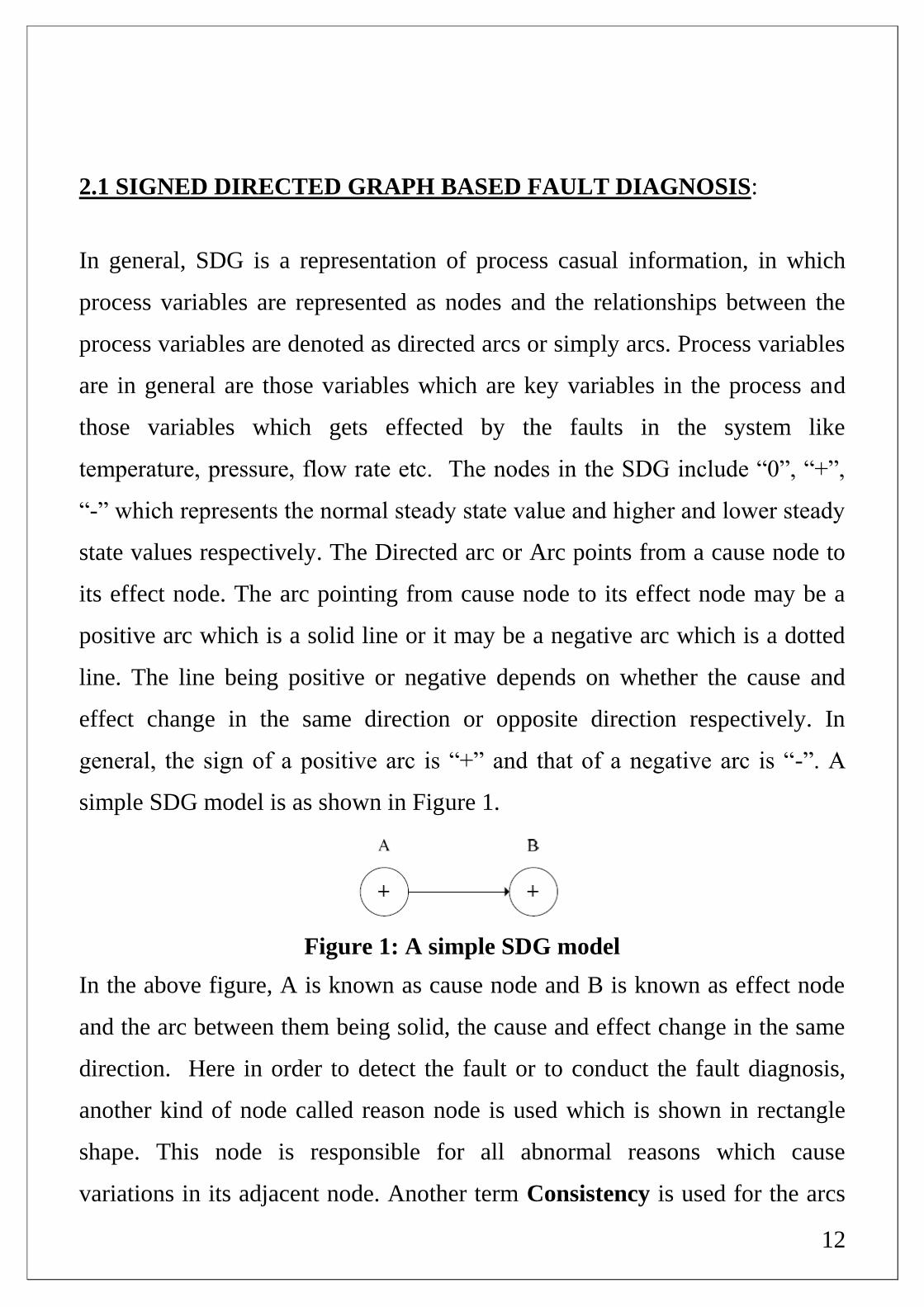
simple SDG model is as shown in Figure 1.
Figure 1: A simple SDG model
In the above figure, A is known as cause node and B is known as effect node
and the arc between them being solid, the cause and effect change in the same
direction. Here in order to detect the fault or to conduct the fault diagnosis,
another kind of node called reason node is used which is shown in rectangle
shape. This node is responsible for all abnormal reasons which cause
variations in its adjacent node. Another term Consistency is used for the arcs

13
which means that an arc is said to be consistent if and only if sign of cause
node *sign of effect node *sign of effect = +. The reason node will have at
least one consistent arc connecting it to an effect node and no such type of
consistent arc to a cause node. If a path is considered as consistent, then it
must have all reason nodes, effect nodes and consistent arcs.
2.1.1 SDG BASED MODELING KNOWLEDGE ON CONTROL
LOOPS:
In many chemical processes, there are many control loops which keeps the
controlled variables at its normal ranges. So, when a fault occurs, control loops
generally protect or mislead the real causes. So hence it is very important to do
the SDG modeling for control loops with utmost care.
Here a tank level control system is taken as an example. It is shown below in
Figure 2.
Figure 2: Simple water tank system
The SDG of the tank level control system is shown in Figure 3. In the Fig, Lm
represents the measuring value of the tank level and LV represents the set
point of the level and LSP is valve. The output flow rate is denoted by F.
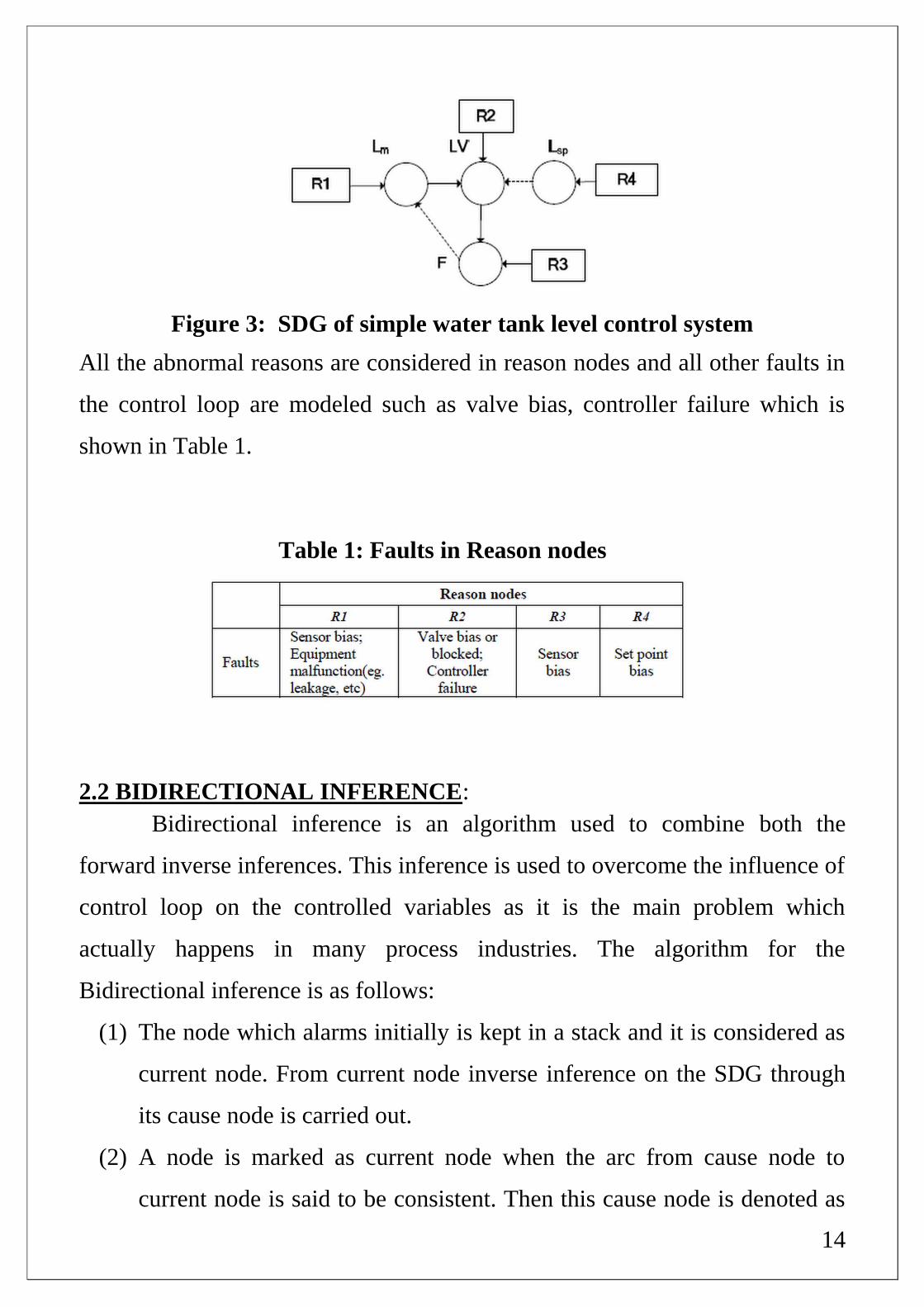
14
Figure 3: SDG of simple water tank level control system
All the abnormal reasons are considered in reason nodes and all other faults in
the control loop are modeled such as valve bias, controller failure which is
shown in Table 1.
Table 1: Faults in Reason nodes
2.2 BIDIRECTIONAL INFERENCE:
Bidirectional inference is an algorithm used to combine both the
forward inverse inferences. This inference is used to overcome the influence of
control loop on the controlled variables as it is the main problem which
actually happens in many process industries. The algorithm for the
Bidirectional inference is as follows:
(1) The node which alarms initially is kept in a stack and it is considered as
current node. From current node inverse inference on the SDG through
its cause node is carried out.
(2) A node is marked as current node when the arc from cause node to
current node is said to be consistent. Then this cause node is denoted as
15
current node and again it is put back into the stack as a current node.
This inference is carried out till the reason node is found out for the
current node.
(3) In the above step if the arc is not consistent, then the cause node will be
observed whether the node is in steady state or the node is the controlled
variable. It is also observed whether the operating variable has been on
the consistent path. It is also to be observed whether the control loop is
influencing the cause node. If it is found to be correct it means that fault
has been propagated through the cause node, but the control loop kept
the cause node in its normal state through its control action. It keeps the
controlled variable normal by making the suitable changes in operating
variable. To find the real root cause, the state of cause node is to be
marked as “+”or “-” making the arc consistent. Then again go for
previous step.
(4) From the reason node found out in the previous step, forward inference
is carried out from the previous node on the path to the abnormal nodes
in the SDG model to predict the states of them. It is just a process of
validation. If the control loops influence the controlled variable, during
the forward inference, if the controlled variable is normal, its state is
supposed to be abnormal. It is assumed to be right if and only if the
states of the abnormal nodes are same with the states predicted.
(5) If there are abnormal nodes being unsearched, then we have to go for
Step no 2, otherwise stop or end the algorithm.
After the above five steps, we will have all the possible causes and the
consistent paths and hence this algorithm will ensure its completeness.
16
In order to develop a SDG, basic knowledge regarding the Digraphs is
required. Hence a case study on Digrpahs has been studied as a part of
literature review.
2.3 CONTROL LOOPS:
In general control loops present in each and every process in which the
essential components are sensor, controller and control device. Through SDGs
the two different types of basic control loops are
a) Negative feedback control loop: Any moderate deviations which occur
in the variables are corrected through this loop. In these loops digraphs
start and end at the same node. It measures the difference between the
set point and output and hence controls the output by comparing it with
the desired value through tis control action.
b) Negative feed forward control loop: As per the theory, any disturbance
created through this loop will cancel out, but this is not practically
possible. It measures the load output directly and hence controls the
output.
In general, negative loops play a key role in many process industries, because
they will stabilize the system. In a positive loop disturbance in one particular
direction will lead to the same disturbance in all other variables and the fault
keeps on multiplying. Hence it is better to have as many numbers of negative
loops as that of positive loops.
Here we have considered an example of a water tank system, courtesy
literature review and through this example the concept of digraph was studied.
17
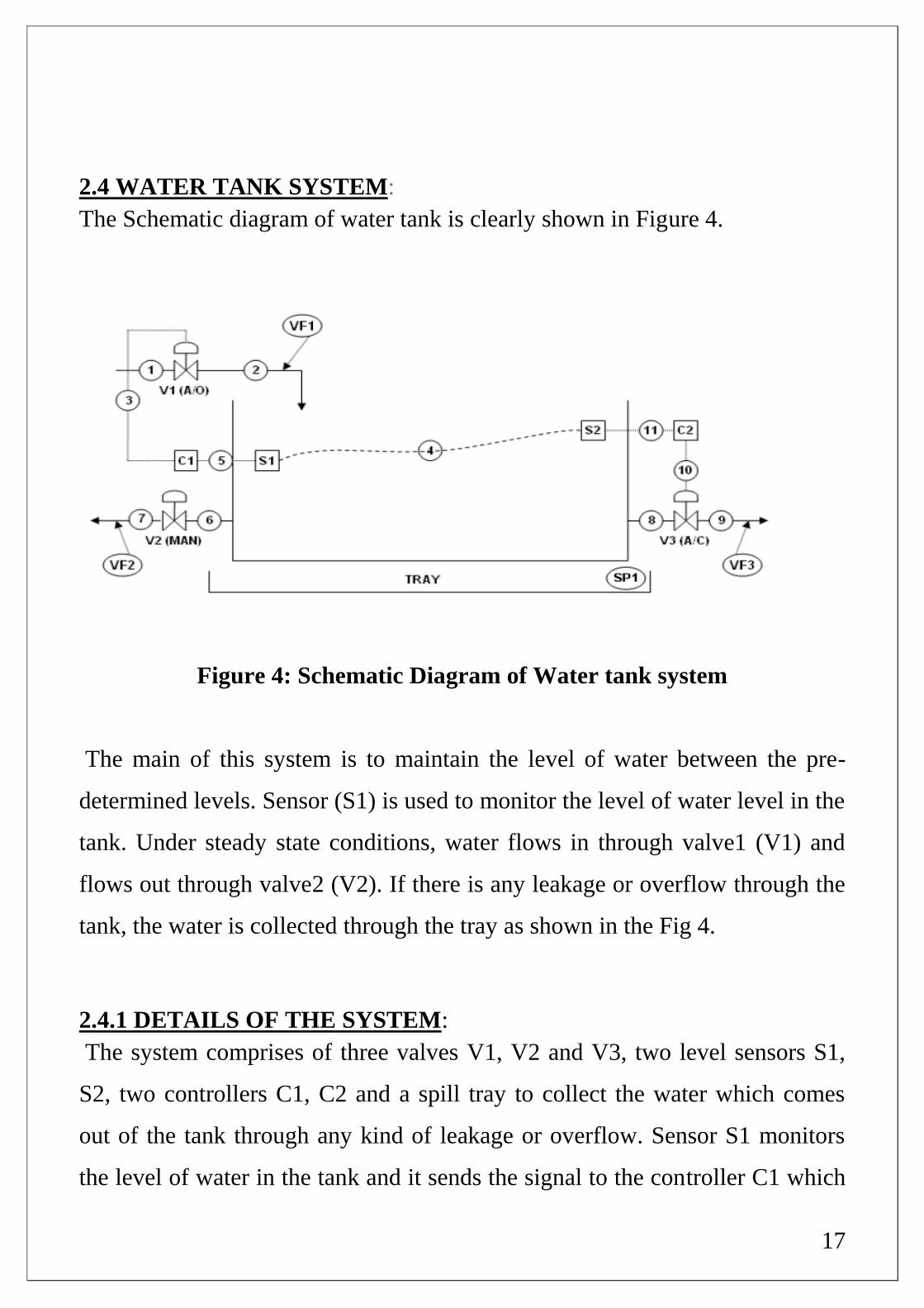
2.4 WATER TANK SYSTEM:
The Schematic diagram of water tank is clearly shown in Figure 4.
Figure 4: Schematic Diagram of Water tank system
The main of this system is to maintain the level of water between the pre-
determined levels. Sensor (S1) is used to monitor the level of water level in the
tank. Under steady state conditions, water flows in through valve1 (V1) and
flows out through valve2 (V2). If there is any leakage or overflow through the
tank, the water is collected through the tray as shown in the Fig 4.
2.4.1 DETAILS OF THE SYSTEM:
The system comprises of three valves V1, V2 and V3, two level sensors S1,
S2, two controllers C1, C2 and a spill tray to collect the water which comes
out of the tank through any kind of leakage or overflow. Sensor S1 monitors
the level of water in the tank and it sends the signal to the controller C1 which
18
in turn controls the valve V1 to control the flow rate of water through V1. It is
maintained in such a way that if the level of the water is more than the desired
level the controller C1 sends a command to the valve to shut down the supply
so that water is drained out and hence maintains the desired level inside the
tank and vice versa. V2 is not associated with any controller since it is
operated manually. In steady state or normal conditions valve V3 is kept
closed as it is considered as a safety valve. If in any case if the controller C1
fails give command to Valve V1 to operate, then sensor S1 senses the level of
water and sends the signal to controller C2 which in turn sends the command
to valve V3 which makes the V3 open and let the excess water out. If there is
any excess water flow in the tank then water will overflow from the tank and
gets collected in the tray provided. The flow sensors will measure the flow
rates through the respective valves. Another sensor SP1 is provided in the tray
to detect whether there is an overflow in the tank.
There are two operating modes for the system. They are
a) Active Mode: In this mode the valves V1 and V2 are kept open and V3
is closed.
b) Dormant Mode: The system is said to be dormant when all the valves
are kept closed.
2.4.2 STEPS FOR DEVELOPING DIGRAPH:
(1) Clearly define the system to be analyzed
(2) Listing out the all possible component failures.
(3) The system is divided into sub units and components.
(4) All control loops present in the system are to be identified.
19
(5) Digraphs of the individual sub units are to be found out by taking into
the consideration all process variable deviations which could have an
effect on the variables present in the model.
(6) All the digraphs of sub systems are connected to form the entire digraph
of the whole system.
(7) Through Back tracing all the possible faults are found out.
2.4.3 ASSUMPTIONS:
The following assumptions are made while constructing the digraph for the
water tank system.
(1) If there is any kind of pipe rupture, flow sensors could not detect it.
(2) The system is in steady state initially
(3) A rupture in the tank causes more leakage of water than the tank
leakage.
2.4.4 WATER TANK DIGRAPH:
Digraphs for the individual sub units are shown in the figures below. Control
loops present in the water tank system are represented as negative feedback
control loops. They are used since they have the ability to correct any kind of
moderate disturbances in any of the process variables.
20
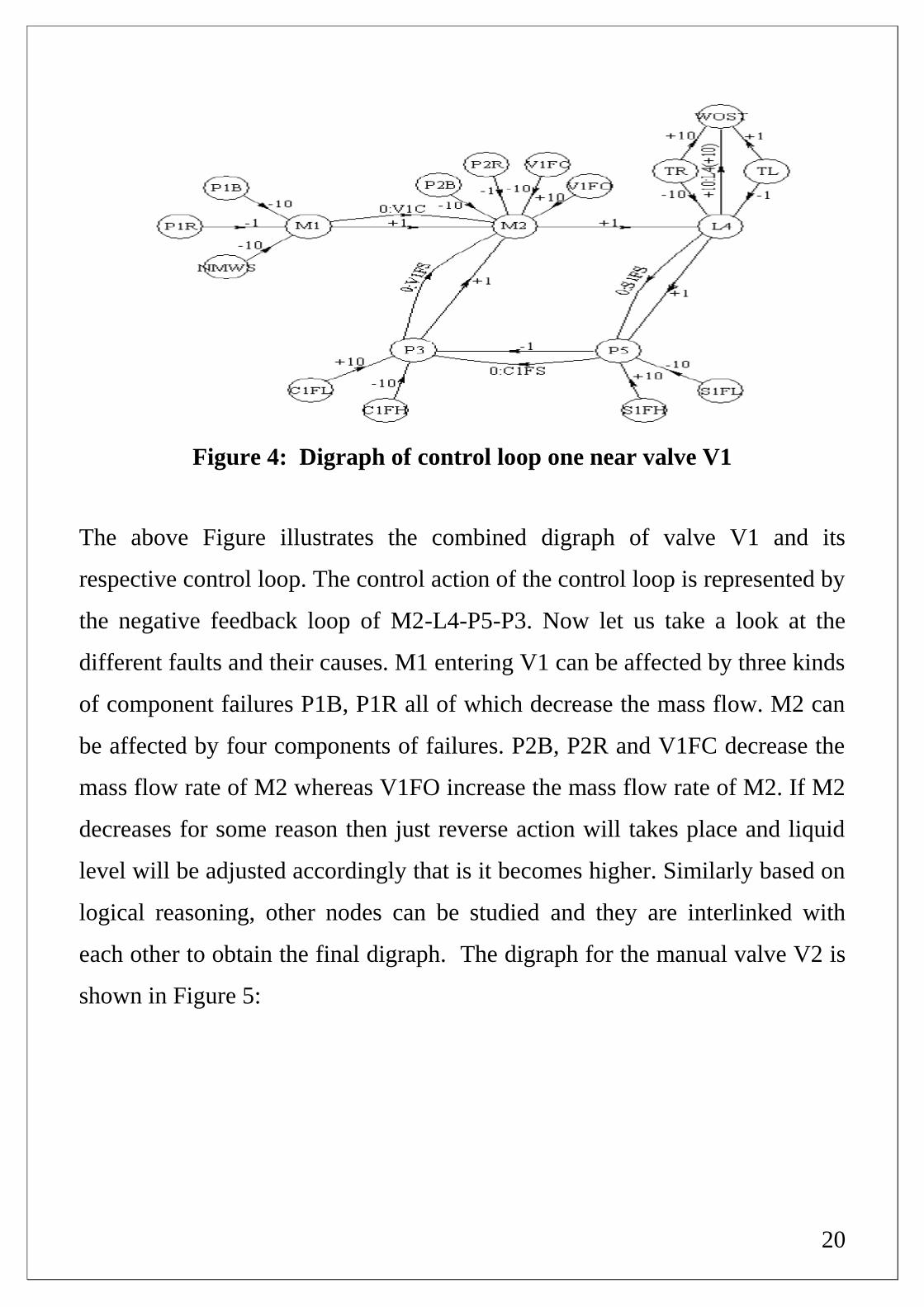
Figure 4: Digraph of control loop one near valve V1
The above Figure illustrates the combined digraph of valve V1 and its
respective control loop. The control action of the control loop is represented by
the negative feedback loop of M2-L4-P5-P3. Now let us take a look at the
different faults and their causes. M1 entering V1 can be affected by three kinds
of component failures P1B, P1R all of which decrease the mass flow. M2 can
be affected by four components of failures. P2B, P2R and V1FC decrease the
mass flow rate of M2 whereas V1FO increase the mass flow rate of M2. If M2
decreases for some reason then just reverse action will takes place and liquid
level will be adjusted accordingly that is it becomes higher. Similarly based on
logical reasoning, other nodes can be studied and they are interlinked with
each other to obtain the final digraph. The digraph for the manual valve V2 is
shown in Figure 5:
21
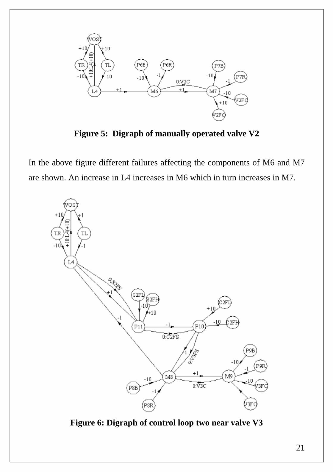
Figure 5: Digraph of manually operated valve V2
In the above figure different failures affecting the components of M6 and M7
are shown. An increase in L4 increases in M6 which in turn increases in M7.
Figure 6: Digraph of control loop two near valve V3
22
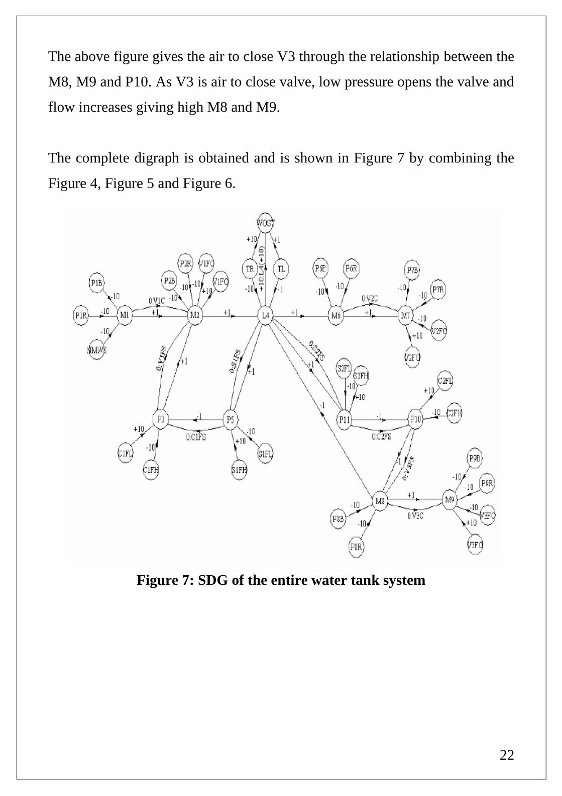
The above figure gives the air to close V3 through the relationship between the
M8, M9 and P10. As V3 is air to close valve, low pressure opens the valve and
flow increases giving high M8 and M9.
The complete digraph is obtained and is shown in Figure 7 by combining the
Figure 4, Figure 5 and Figure 6.
Figure 7: SDG of the entire water tank system
23
2.4.5 FAULT DIAGNOSTIC METHODS:
For fault diagnosis, the system sensor readings are compared with the
expected values when the system is in operating mode. If at all a node registers
a deviation, diagnosis involves back tracing from the node through which it is
possible to determine the failure nodes. Back tracing is done in two ways.
Method one: Back tracing is done from the fault node until the point where
there is no further back tracing can be done. The main disadvantage associated
with this is many faults will be generated and most of them seems to be
contradictory and hence creates an ambiguity.
Method two: From sensor readings it is observed that which particular areas
is showing deviation and that particular area is flagged off leaving behind the
non-deviating nodes. Back tracing from a node stops as soon as it reaches the
boundary of the flagged section.
Let us consider an example of method two. A deviation from the normal active
mode in which VF1 and VF2 showing no flow of water through the valves.
Since there is no problem with VF3 or SP1, this particular section can be
flagged off. No flow in V1 will cause M2 to decrease which can be caused by
P2B, P2R and V1FC. It will also be caused by a decrease in M1 which in turn
caused by P1R, P1B. If we go through the control loop, decrease in M2 will
also be registered due to high liquid level through L4.
Following chapters are based on the control systems and water tank problems
that have been studied as a part of this project and their SDGs and Fuzzy SDG
are developed.
24
Chapter – 03
FEEDBACK CONTROL
SYSTEM
25
3.1 CONTROL SYSTEMS:
Control systems often play a very important role in many chemical processing
industries. The main aim of these control systems in industries is to control the
process variables such as temperature, pressure, flow rate etc. Control actions
should be considered particularly because they are the forced actions which are
different from the process itself and they are responsible for misleading of the
fault propagation. Here in this chapter different types of control systems are
considered and their SDGs are developed with the help of the existing
theoretical and process knowledge.
3.2 FEED BACK CONTROL SYSTEM:
Feed Back Control systems play a very important role in process control
system industries. Typical feedback control system is shown in Fig 9. In
feedback control systems the variable which is to be controlled is measured
and it is compared with the desired value. The difference between the actual
value and the desired set point is called error. Feedback control system tries to
reduce the error by adjusting or manipulating the input value to the system.
3.2.1 SYSTEM DESCRIPTION:
In the below figure,
r = desired set point
e = error
u = controller output
x = controlled variable
q = manipulated variable
xm = measurement of final controlled output
26
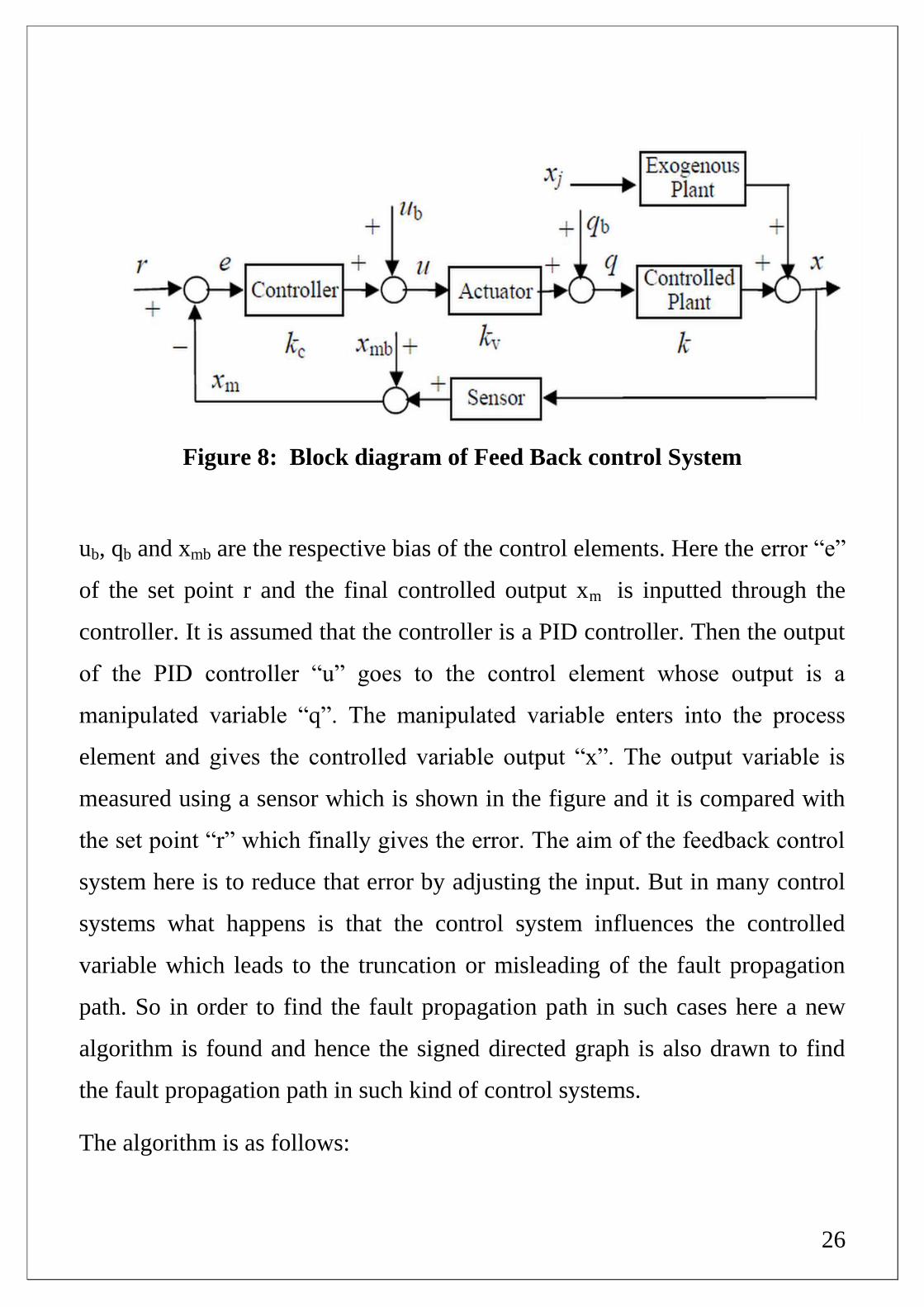
Figure 8: Block diagram of Feed Back control System
ub, qb and xmb are the respective bias of the control elements. Here the error “e”
of the set point r and the final controlled output xm is inputted through the
controller. It is assumed that the controller is a PID controller. Then the output
of the PID controller “u” goes to the control element whose output is a
manipulated variable “q”. The manipulated variable enters into the process
element and gives the controlled variable output “x”. The output variable is
measured using a sensor which is shown in the figure and it is compared with
the set point “r” which finally gives the error. The aim of the feedback control
system here is to reduce that error by adjusting the input. But in many control
systems what happens is that the control system influences the controlled
variable which leads to the truncation or misleading of the fault propagation
path. So in order to find the fault propagation path in such cases here a new
algorithm is found and hence the signed directed graph is also drawn to find
the fault propagation path in such kind of control systems.
The algorithm is as follows:

27
(1) From the existing theoretical knowledge we need to develop a block
diagram and then all the equations associated with the control system are
to be found out.
(2) Relations between the variables needs to be found out such that whether
a change in variable causes positive, negative or neutral effect on the
adjacent or related variable.
(3) Then the Signed Directed Graph is drawn basing on the process
knowledge and the fault propagation path is found out by using the
equations and process knowledge and with logical reasoning.
By using the control law of the feedback control system, the various
equations involved are:
xm = x+ xmb (1)
e = r- xm (2)
up = kce (3)
(d/dt)uI = kce/τI (4)
uD = kcτD(de/dt) (5)
u= up+ uI + uD + ub (6)
q = kvu+qb (7)
x = kq+ajxj (8)
Here aj and xj are the additional gain and external disturbance of the
exogenous plant as shown in the figure above. τI and τD are the integral and
differential time constant respectively. Basing on the above equations the
relationship the variables can be found out whether a positive or negative or
neutral effect is existing between the variables which are connected through

28
the equations. Table 2 shows the perfectly matching variables using the
above equations.
Table 2: Matched variables
Equation Variables with “+”cause and
effect
1 xmb and x
2 e and xm
3 up and e
5 ud and ud
6 u and up
7 q and u
8 x and q
Figure 9: SDG of the system
29
In the above SDG shown the nodes which are denoted with dotted lines are
deviation nodes and the arrows with solid line represent the positive effect the
variables and the arrows with the dotted line represents the negative effect
present between the variables. Since we have considered that the controller is a
PID controller up, uI and uD are drawn as three separate nodes because their
effect changes with respect to time. We can also say that the above SDG is
drawn considering the initial response of the system. That is the reason why uI
is marked with “0”, since during the initial response the integral controller will
not have that much effect. Hence its effect is considered to be negligible. Also
the effect of de/dt is considered as a node because of its special effect on uD.
But its effect is limited to only during the initial response itself. Using the
above SDG, the initial response can be analyzed. If the set point r is decreased
then the corresponding nodes e, up, u, q, xm and x will have the same positive
effect and these nodes will also show a decrease in their corresponding
measurement and the corresponding value of uI will decrease immediately
because there is a direct arc connecting from e to uI. Also it is found that the
propagation path is consistent. So after finding SDG what we can infer form
here is that the fault propagation path of the initial response of the feedback
control system is the longest acyclic path, in which fault origination path will
start from its desires set point. The actual fault propagation path will be “set
point → error → manipulated variable → controlled output → measured
value → error”. Also it is found that the path is consistent.
In steady state the value of error is zero in the final response. Since the value
of error “e = 0” in this case, both the values of up and uD are zero. In order to
form SDG again we need to develop the differential algebraic equations by
using the process knowledge and logical reasoning. The above DAE’s will
change and the new equations are as follows:

30
xm = x + xmb (9)
xm = r (10)
u = uI + ub (11)
q = kvu + qb (12)
x = kq+ajxj (13)
From the above equations we can easily find the relationship between the
process variables and these are tabulated in Table 2. After forming the tables it
is easy to draw the SDG and then fault propagation paths are found out.
Table 3: Matched variables when system is at steady state
From the above table we can easily draw the SDG of the system and it is
shown in Figure 10 as follows:
Equation
Variables with “+” cause and
effect
(9) xm and x
(10) r and xm
(11) u and uI
(12) q and u
(13) x and q
31
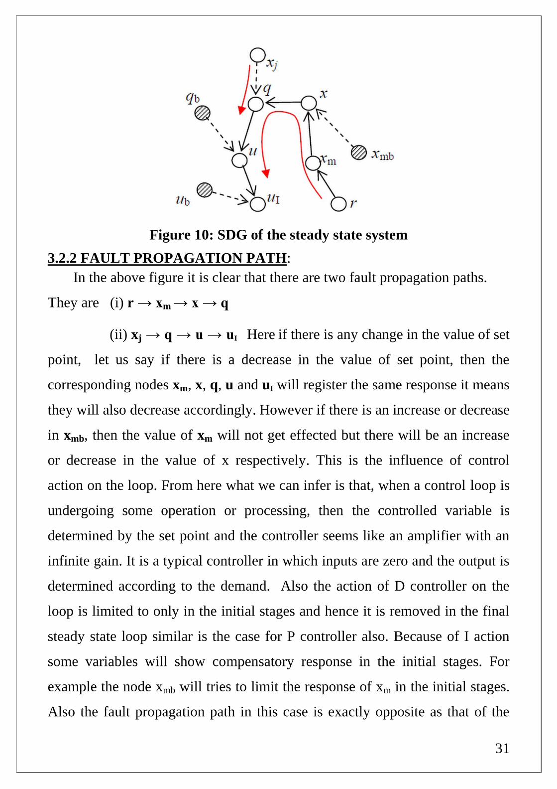
Figure 10: SDG of the steady state system
3.2.2 FAULT PROPAGATION PATH:
In the above figure it is clear that there are two fault propagation paths.
They are (i) r → xm → x → q
(ii) xj → q → u → uI Here if there is any change in the value of set
point, let us say if there is a decrease in the value of set point, then the
corresponding nodes xm, x, q, u and uI will register the same response it means
they will also decrease accordingly. However if there is an increase or decrease
in xmb, then the value of xm will not get effected but there will be an increase
or decrease in the value of x respectively. This is the influence of control
action on the loop. From here what we can infer is that, when a control loop is
undergoing some operation or processing, then the controlled variable is
determined by the set point and the controller seems like an amplifier with an
infinite gain. It is a typical controller in which inputs are zero and the output is
determined according to the demand. Also the action of D controller on the
loop is limited to only in the initial stages and hence it is removed in the final
steady state loop similar is the case for P controller also. Because of I action
some variables will show compensatory response in the initial stages. For
example the node xmb will tries to limit the response of xm in the initial stages.
Also the fault propagation path in this case is exactly opposite as that of the
32
initial response case. So we can finally conclude this study with two cases.
They are (i) When control loop operates then the fault propagation will be due
to the deviation of sensor, or other external disturbances.
(ii) When control loop does not operate we will have two cases
through which fault may propagate. They are (1) structural faults (2) excessive
deviation which causes the controller saturation which automatically leads to
the error = zero.
33
Chapter – 04
CASCADE CONTROL SYSTEM

34
4.1 INTRODUCTION:
Cascade Control system can be considered as an extension of a single loop
control. The main advantage of cascade control system is that it will improve
the performance of control system over a single loop control whenever either
the measurable intermediate value is getting affected by the disturbances or
when the primary process output that we needs to control gets directly affected
by the secondary process output. In this case cascade control system can limit
the effect of disturbances entering into the secondary variable on the primary
output. The main application of cascade control systems is seen in case of shell
and tube heat exchangers.
4.1.1 SYSTEM DESCRIPTION:
Figure 11: Block Diagram of Cascade Control System
In the above figure we have two loops in which e1 is the error of the outer loop
and e2 is the error in the inner loop and all other variables are given same
meaning as that in the previous case of feedback control system. To construct
SDG we need to follow the same algorithm as said before. In order to form
SDG again we need to form all the equations by using the process knowledge.
35
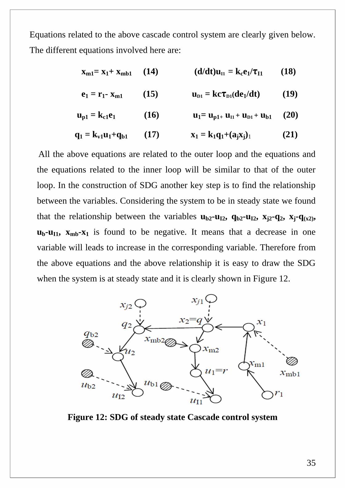
Equations related to the above cascade control system are clearly given below.
The different equations involved here are:
xm1= x1+ xmb1 (14) (d/dt)uI1 = kce1/τI1 (18)
e1 = r1- xm1 (15) uD1 = kcτD1(de1/dt) (19)
up1 = kc1e1 (16) u1= up1+ uI1 + uD1 + ub1 (20)
q1 = kv1u1+qb1 (17) x1 = k1q1+(ajxj)1 (21)
All the above equations are related to the outer loop and the equations and
the equations related to the inner loop will be similar to that of the outer
loop. In the construction of SDG another key step is to find the relationship
between the variables. Considering the system to be in steady state we found
that the relationship between the variables ub2-uI2, qb2-uI2, xj2-q2, xj-q(x2),
ub-uI1, xmb-x1 is found to be negative. It means that a decrease in one
variable will leads to increase in the corresponding variable. Therefore from
the above equations and the above relationship it is easy to draw the SDG
when the system is at steady state and it is clearly shown in Figure 12.
Figure 12: SDG of steady state Cascade control system
36
4.1.2 FAULT PROPAGATION PATH:
From the above figure what we can infer is that there are three fault
propagation paths similar to that of the feedback control system.
They are (i) r1→xm1→x1→x2→xm2→u1→uI1
(ii) xj1→x2→xm2→r1→uI1
(iii) xj2→q2→u2→uI2---- ub2
In the above figure the nodes which are marked with dotted lines are
deviation nodes. These nodes are based on the bias that produced in the
system. Initially a change in the node xmb1 will affect the final measurement
output variable xm1. But later, it means when the system is in steady state it
is not happening because the control action misleads the fault propagation
path. Thus all the propagation paths are successfully found out. If we
consider the same system during its initial stage, then the initial response
SDG will look similar to that of the SDG except that there won’t be any kind
of breaking of links between the nodes and another two extra nodes will be
there for representing the errors present in the inner and outer loop
respectively. The path in the initial response will be opposite to the path of
the steady state path. In almost all process industries faults will generally
occur when the system is at steady state itself. For us it seems like that the
system is in steady state but because of the influence of the control loop it
will mislead the path. Hence from now onwards SDG of the other control
systems were drawn considering the system is at steady state.
37
Chapter – 05
TWO ELEMENT CONTROL
SYSTEM
38
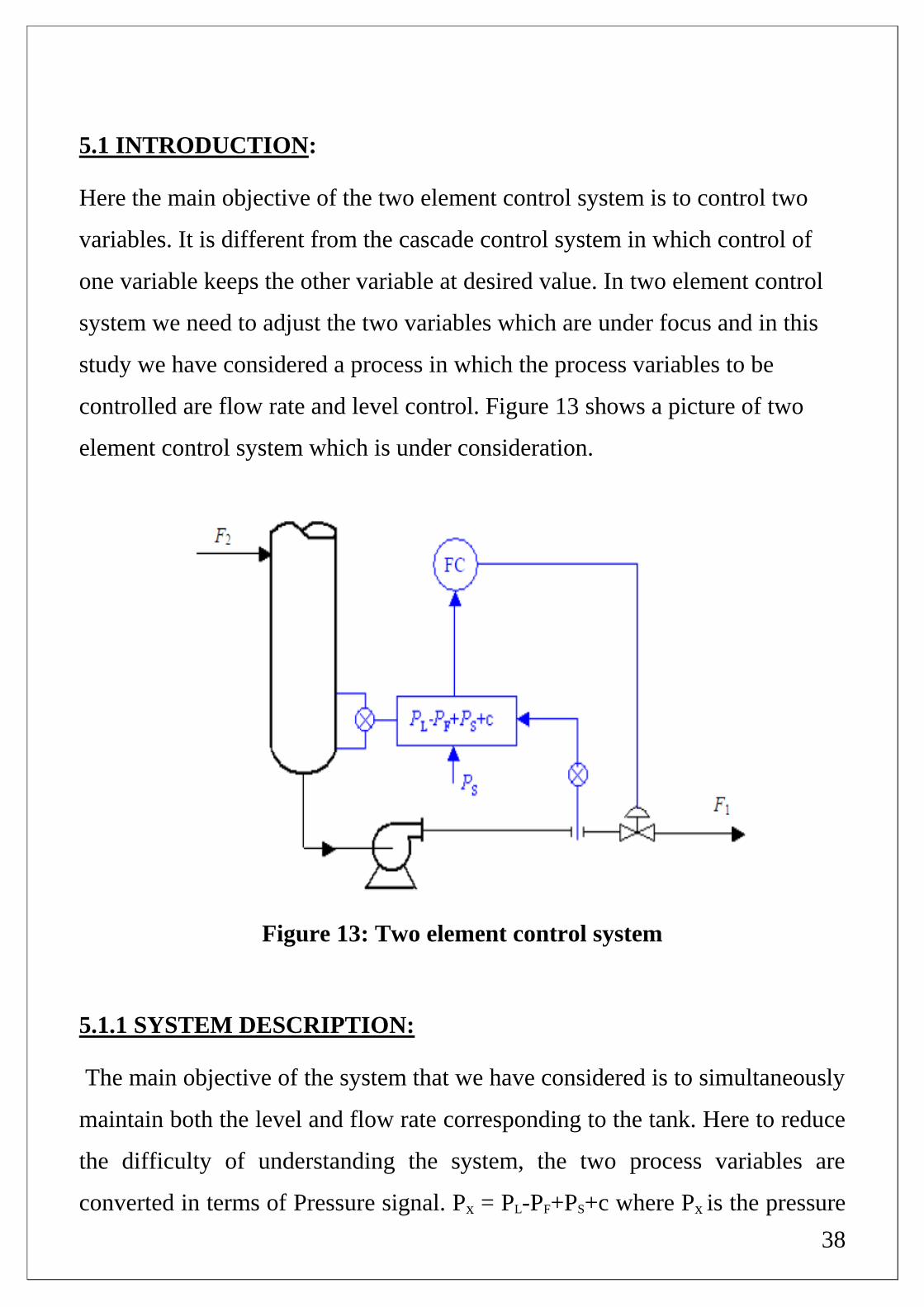
5.1 INTRODUCTION:
Here the main objective of the two element control system is to control two
variables. It is different from the cascade control system in which control of
one variable keeps the other variable at desired value. In two element control
system we need to adjust the two variables which are under focus and in this
study we have considered a process in which the process variables to be
controlled are flow rate and level control. Figure 13 shows a picture of two
element control system which is under consideration.
Figure 13: Two element control system
5.1.1 SYSTEM DESCRIPTION:
The main objective of the system that we have considered is to simultaneously
maintain both the level and flow rate corresponding to the tank. Here to reduce
the difficulty of understanding the system, the two process variables are
converted in terms of Pressure signal. Px = PL-PF+PS+c where Px is the pressure
39
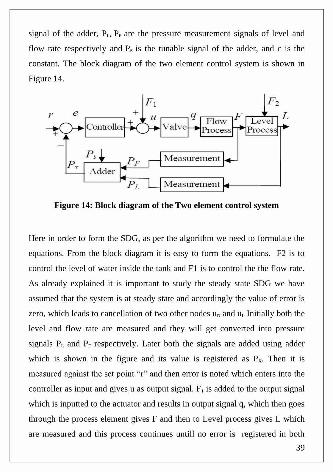
signal of the adder, PL, PF are the pressure measurement signals of level and
flow rate respectively and PS is the tunable signal of the adder, and c is the
constant. The block diagram of the two element control system is shown in
Figure 14.
Figure 14: Block diagram of the Two element control system
Here in order to form the SDG, as per the algorithm we need to formulate the
equations. From the block diagram it is easy to form the equations. F2 is to
control the level of water inside the tank and F1 is to control the the flow rate.
As already explained it is important to study the steady state SDG we have
assumed that the system is at steady state and accordingly the value of error is
zero, which leads to cancellation of two other nodes uD and uI. Initially both the
level and flow rate are measured and they will get converted into pressure
signals PL and PF respectively. Later both the signals are added using adder
which is shown in the figure and its value is registered as PX. Then it is
measured against the set point “r” and then error is noted which enters into the
controller as input and gives u as output signal. F1 is added to the output signal
which is inputted to the actuator and results in output signal q, which then goes
through the process element gives F and then to Level process gives L which
are measured and this process continues untill no error is registered in both

40
level and flow rates. The equations corresponding to the steady state system
are: e = r - PX (22)
u + F1 = k.q (23)
SDG of the two element control system is shown clearly in the Fig 16. In the
figure it is clear that the level and flow have both positive and negative effects
which is different from that of the cascade control system. Also in this case F1
is registered as a deviation node and an incease in F1 will register a decrease in
the value of uI .
Figure 15: SDG of steady state Two element control system
5.1.2 FAULT PROPAGATION PATH:
From the above Steady state SDG it is easy to find the fault propagation paths.
It is clear that there are two fault propagation paths and they are
(i) r→ PX→L → F →q
(ii) F2 →F→L & F2→F→q→u→uI
Thus SDG of the two element control system and the fault propagations paths
were determined. Based on this result it is easy to find the SDG’s and fault
propagation paths of various complex control systems. They can be obtained
by the combination of several single control loops or sometimes the
combination and connection of single and cascade control loops.

41
Chapter – 06
THREE ELEMENT CONTROL
SYSTEM
42
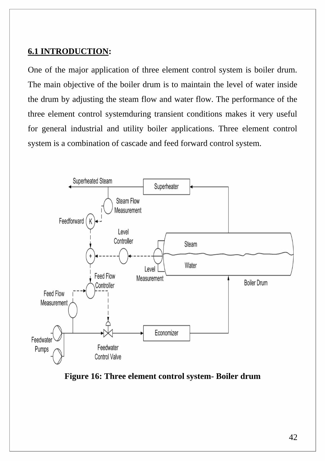
6.1 INTRODUCTION:
One of the major application of three element control system is boiler drum.
The main objective of the boiler drum is to maintain the level of water inside
the drum by adjusting the steam flow and water flow. The performance of the
three element control systemduring transient conditions makes it very useful
for general industrial and utility boiler applications. Three element control
system is a combination of cascade and feed forward control system.
Figure 16: Three element control system- Boiler drum
43
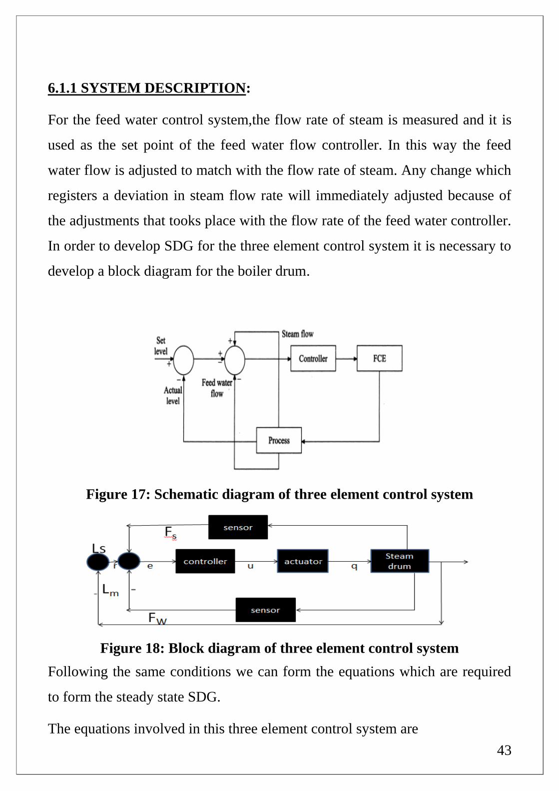
6.1.1 SYSTEM DESCRIPTION:
For the feed water control system,the flow rate of steam is measured and it is
used as the set point of the feed water flow controller. In this way the feed
water flow is adjusted to match with the flow rate of steam. Any change which
registers a deviation in steam flow rate will immediately adjusted because of
the adjustments that tooks place with the flow rate of the feed water controller.
In order to develop SDG for the three element control system it is necessary to
develop a block diagram for the boiler drum.
Figure 17: Schematic diagram of three element control system
Figure 18: Block diagram of three element control system
Following the same conditions we can form the equations which are required
to form the steady state SDG.
The equations involved in this three element control system are
44
(i) Ls-Lm = r (24)
(ii) e = k.u (25)
(iii) u = kv.q (26)
Here k and kv are the the positive gains of the control elements respectively.
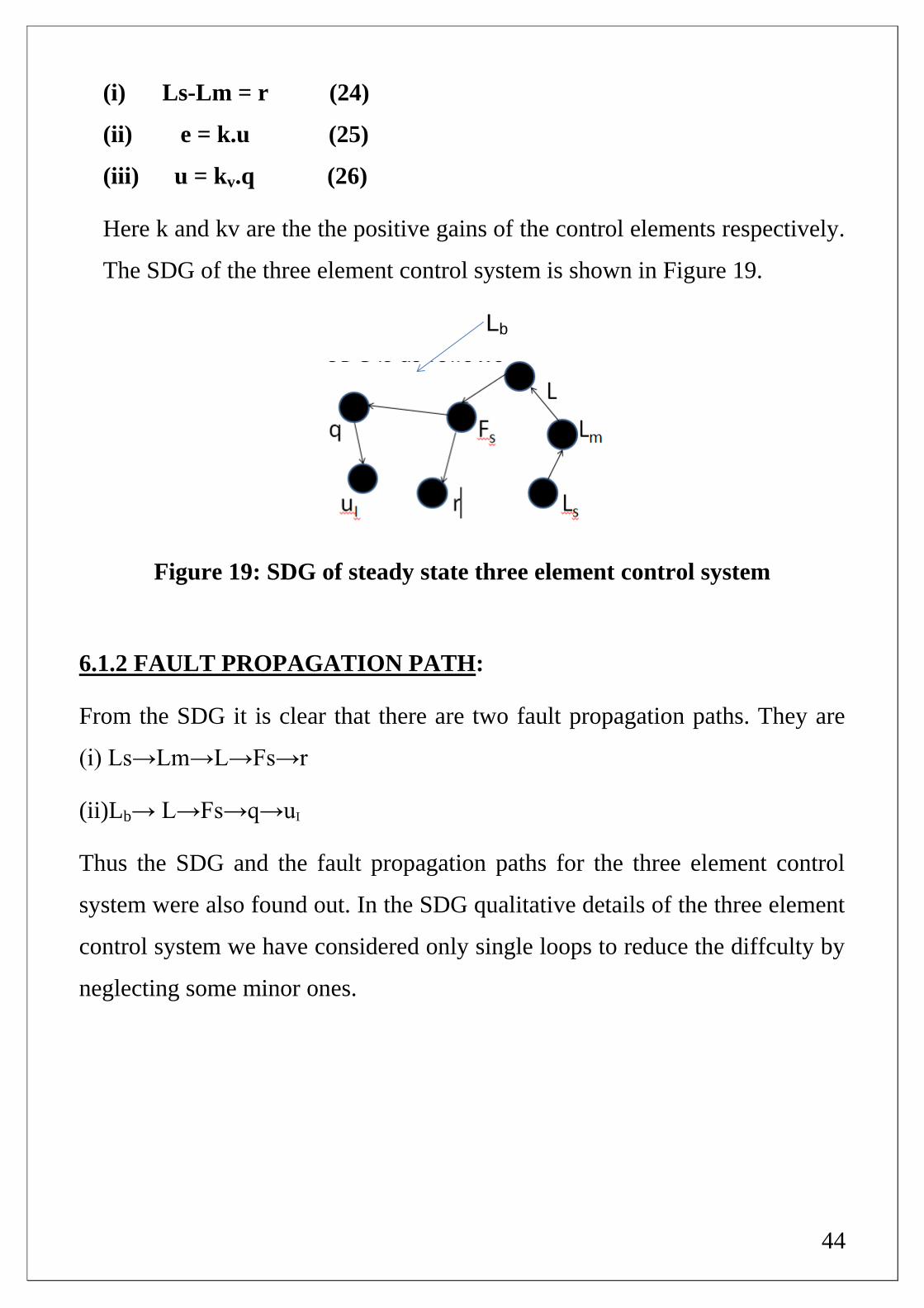
The SDG of the three element control system is shown in Figure 19.
Lb
Figure 19: SDG of steady state three element control system
6.1.2 FAULT PROPAGATION PATH:
From the SDG it is clear that there are two fault propagation paths. They are
(i) Ls→Lm→L→Fs→r
(ii)Lb→ L→Fs→q→uI
Thus the SDG and the fault propagation paths for the three element control
system were also found out. In the SDG qualitative details of the three element
control system we have considered only single loops to reduce the diffculty by
neglecting some minor ones.

45
Chapter – 07
FUZZY LOGIC
46
7.1 FUZZY SIGNED DIRECTED GRAPH:
7.1.1 DEFINITION:
The concept of fuzzy graph is a natural generalisation of the crisp graphs using
fuzzy sets. A crisp graph is denoted by the pair G = (X,E) where X is a finite
set of nodes and E a non fuzzy relation on X x X. A fuzzy graph is a pair (X’,
E’ ), where X’ is a fuzzy set on X and E’ is a fuzzy relation on X x X’ such
that µE < min (µX’(x), µX’(x’)). Here µE is the membership function of the
binary effect of two adjacent nodes x and x’ over a branch µX’, the mebership
function of the node. However, in some situations it may be desirable to relax
this ineqality. If µE’ and µX’ only take the values of -1,0 or 1, then a fuzzy graph
becomes crisp.
7.2 NODES:
Each node in a fuzzy-SDG is represented by a fuzzy variable. An example of
value space of a node is considered. The number of fuzzy values covered by
the fuzzy value space is determined by the problem requirements. It is worth
noting that the method is not restricted to a three range pattern of -,+,0. Every
legal value of node variable such as high and medium high is a fuzzy set M’.
M’ is therefore represented by its membership function, µ, such that the value
of µ illustrates the degree of membership of the element x belonging to M’.
whether a value of x belongs to M’ depends on both the value of µ and the ƛ
cut value of M’. the membership function, may take various shapes but the
most common is the triangular and trapezoidal representations. In fuzzy signed
directed graphs, node is uniquely defined by the following expression
Node_name (val, µ,ʋ, type, arrow-to-node-list,arrow-from-node-list)
47
In the above expression val represents the value of node such as high or low; ʋ
is the smoothed valuein [-1,-1], of the real value of the variable such as 0.60
corresponding to 1.6 m for liquid level, µ is the membership function value,
arrow to node list is the list of all node names to which this node points to and
arrow from nodes list includes all node names from which the current node is
being pointed to; type is the type of variable. A process variable can be one of
the three types of variables: they are controlled level such as the liquid level
shown in Fig 1. Measured variables such as flowrate and unmeasured variable
such as valve opening. All controlled variables are measured variables.
7.3 WORKING WITH FUZZY LOGIC TOOL BOX:
The fuzzy logic tool box provides different types of GUIs to let us perform
various classical fuzzy system development and pattern recognition. Using the
fuzzy tool box, we can
(i) Develop and analyze fuzzy inference systems
(ii) Develop adaptive neuofuzzy inference systems.
(iii) Perform fuzzy clustering.
In addition, the toolbox provides a fuzzy controller block that we can use in
Simulink to model and simulate a fuzzy logic control system.
7.4 BUILDING A FUZZY INFERENCE SYSTEM(FIS):
Fuzzy inference is a method that interprets the values in the input vector and
based on user defined rules, it will assign values to the output vector. Using
the GUI editors and viewers in the Fuzzy Logic Toolbox, we can build the
rules set, define the membership functions and analze the behavior of FIS.
The following editors and viewers are provided.

48
(i) FIS editor: It displays the general information about the Fuzzy
inference system
(ii) Membership function editor: Lets you display and edit the
membership functions associated with the input and output variables
of FIS.
(iii) Rule Editor: It will help us in viewing and editing of Fuzzy rules
using one of the three formats. Full English-like syntax, concise
symbolic notation, or an indexed notation.
(iv) Rule viewer: It will give detailed behavior of FIS to help diagnose
the behavior of specific rules or study the effect of changing input
variables.
(v) Surface viewer: It generates a 3-D surface from two input variables
and the output of an FIS.
In order to simulate fuzzy logic controller we need to develop an algorithm.
The algorithm is as follows:
(i) For a given fuzzy logic controller or system we need to mention the
number of inputs and number of outputs.
(ii) Each and every input and output is to be defined by some particular
membership functions.
(iii) We need to develop the appropriate rules using experence and
knowledge.
(iv) After defining rules, the only step remaining is to do simulation and to
conduct the fault analysis.
To understand a simple system was initally studied.
49
7.5 CASE STUDY- CSTR:
Let us consider a simple example of jacketed CSTR in which a simple
reaction A + B → C. Here in this system there are two inputs and one
output. Before going to simulate this model, we need to predefine the
objective of the problem. Basing on the amount of both A and B reacted we
will have the output product C. We will define the range of the output
product C on the basis of 10 point scale. Before going to do the simulation
we need to define the cases. Here we have consider three cases.
They are:
(i) If the amount of reactants A & B is less, then the amount of product
formed is less.
(ii) If the amount of reactant A is average, irrespective of B,then the
amount of product formed is medium.
(iii) If both the amounts of reactants reacted are large,then the amount of
product formed C is also large. In terms of fuzzy logic it is excellent.
After defining the three cases, we can go for simulation. As per the
algorithm we have already mentioned the number of inputs and number of
outputs in the system. In this case there are two inputs and two outputs in
our system. In the command space of the Matlab type fuzzy . After entering
this command , Matlab will open a FIS editor which is shown in Fig 21. In
default window it seems that there are one input one system and another
output. we need to add one more input through the edit tab placed in the FIS
editor.Then after adding input the FIS editor,it will change as shown in
Figure 21. Finally we have two inputs and one output and next thing to do is
defining the inputs and then the membership functions. We can directly
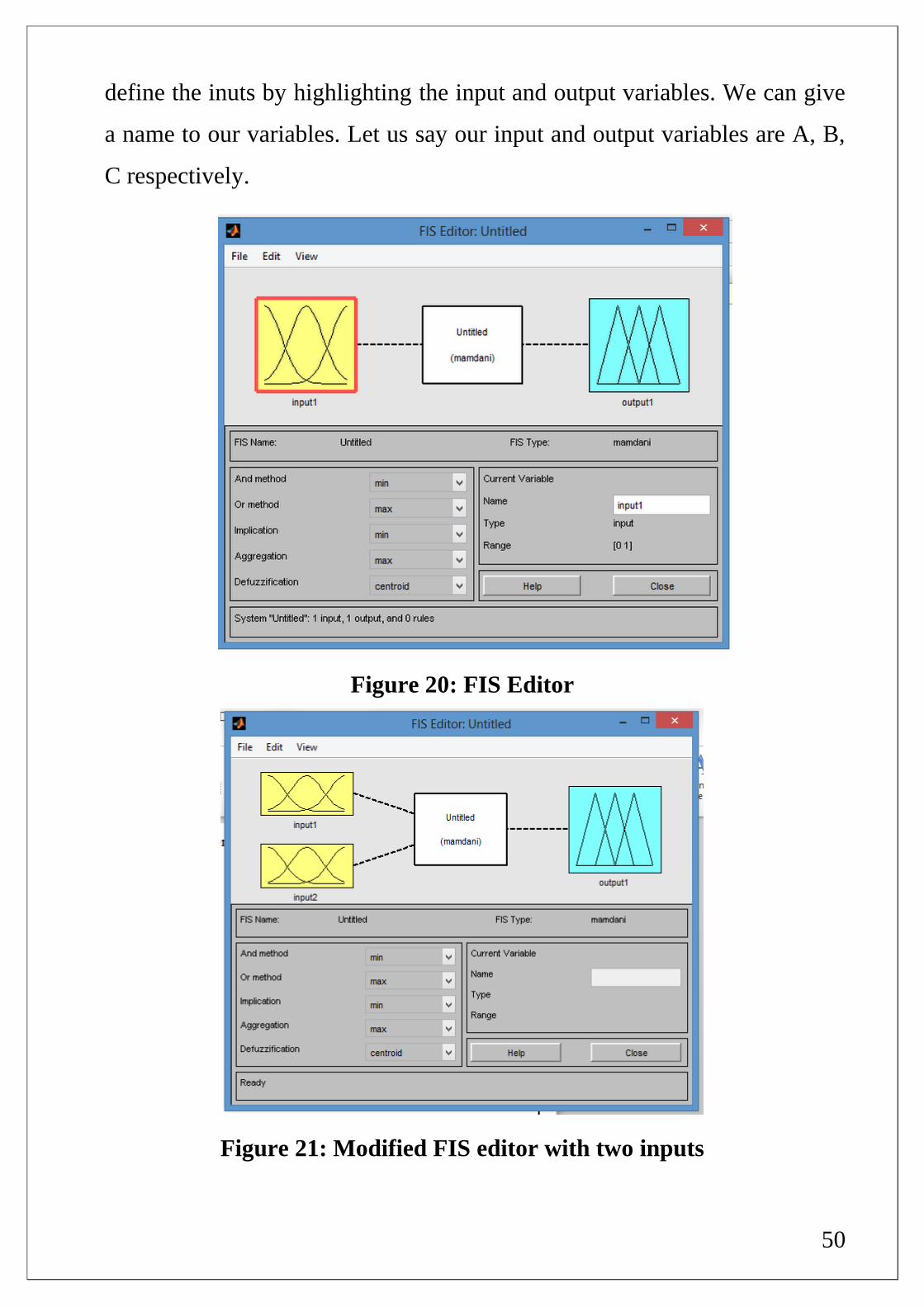
50
define the inuts by highlighting the input and output variables. We can give
a name to our variables. Let us say our input and output variables are A, B,
C respectively.
Figure 20: FIS Editor
Figure 21: Modified FIS editor with two inputs
51
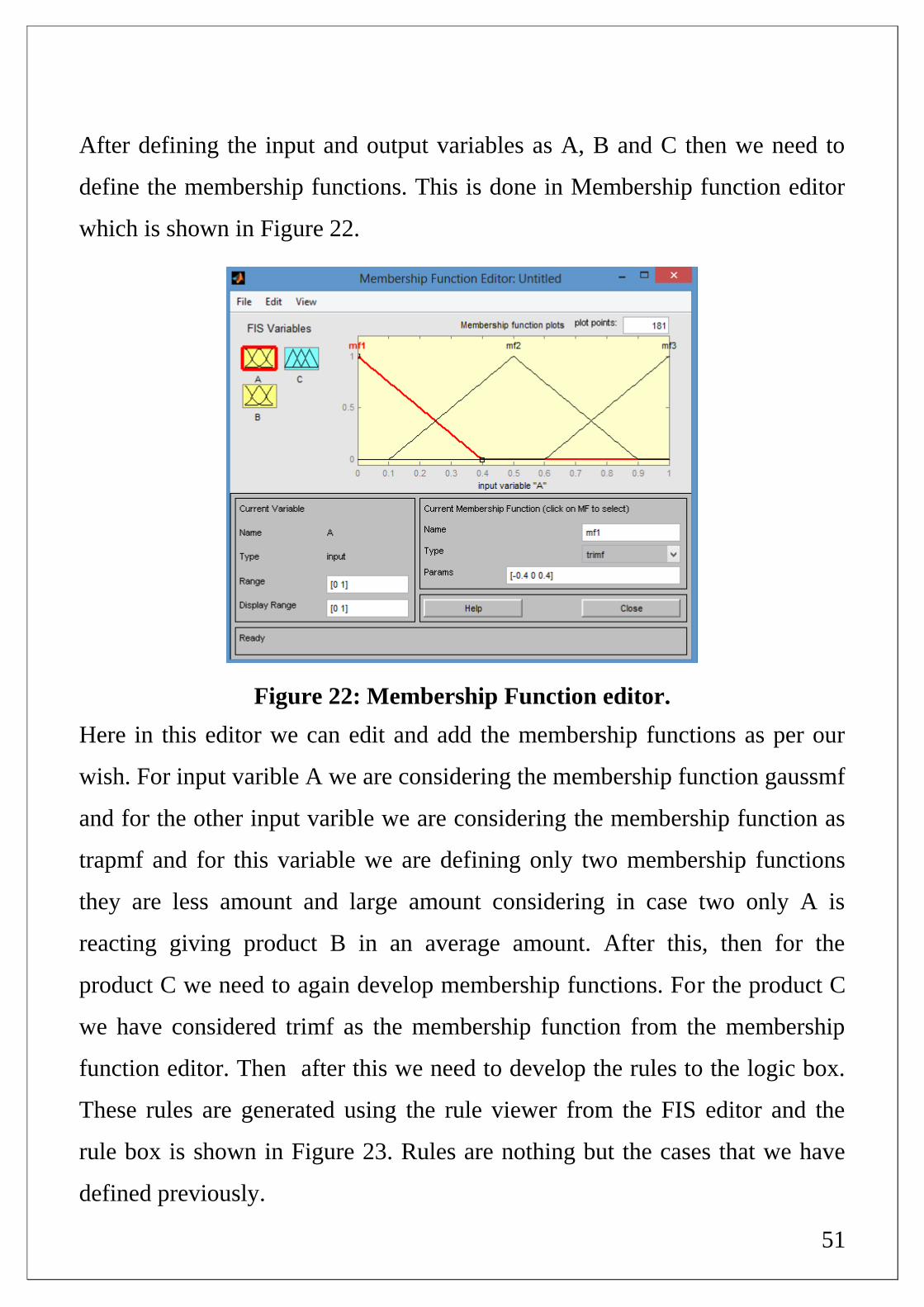
After defining the input and output variables as A, B and C then we need to
define the membership functions. This is done in Membership function editor
which is shown in Figure 22.
Figure 22: Membership Function editor.
Here in this editor we can edit and add the membership functions as per our
wish. For input varible A we are considering the membership function gaussmf
and for the other input varible we are considering the membership function as
trapmf and for this variable we are defining only two membership functions
they are less amount and large amount considering in case two only A is
reacting giving product B in an average amount. After this, then for the
product C we need to again develop membership functions. For the product C
we have considered trimf as the membership function from the membership
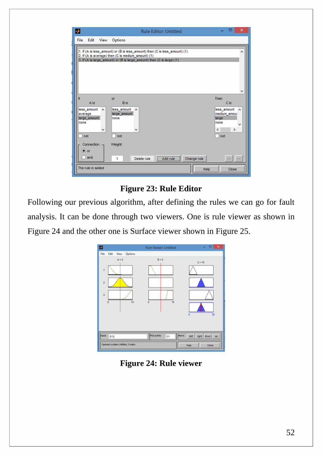
function editor. Then after this we need to develop the rules to the logic box.
These rules are generated using the rule viewer from the FIS editor and the
rule box is shown in Figure 23. Rules are nothing but the cases that we have
defined previously.
52
Figure 23: Rule Editor
Following our previous algorithm, after defining the rules we can go for fault
analysis. It can be done through two viewers. One is rule viewer as shown in
Figure 24 and the other one is Surface viewer shown in Figure 25.
Figure 24: Rule viewer

53
Figure 25: Surface viewer.
By changing the values in rule viewer we can easily find how the output is
getting affected by the input variables. Even in complex scale industries once
if we define the number of inputs and number of outputs it will be easy for us
to say how the output gets effected by a particular variable. It gives us a good
logical reasoning in fault diagnosis. Using Fuzzy SDG will definitely reduce
the time required to do fault diagnosis and also we can easily validate the
results in case of Fuzzy SDG.
Table 4: Effect of input variables on the output variables
Amount of A Amount of B Amount of C
5 5 15
2 2 8
7 7 16
8.5 9 25
9.5 10 26
54
Chapter – 08
CONCLUSIONS
&
RECOMMENDATION
55
8.1 CONCLUSION AND RECOMMENDATION:
The advantages of Signed Directed graph are
(i) The SDG method discusses in detail the various possible faults that
might happen in the system and the fault propagation paths through
which fault is propagated, thus giving a proper analysis of the system.
(ii) Fault can be traced back to its root cause using Inverse inference
mechanism or by using the Bidirectional inference.
(iii) SDG, once fully developed and validated using some theories or
simulation programs, then it is so easy to study and even ordinary
workers in process industries can understand without any special
education. They can easily carry out the fault detection and analysis by
having proper SDG of the process system.
The main Disadvantages of Signed Directed Graph are:
(i) SDG gives qualitative analysis. The deviations in the process variables
are assigned the states of high, low or steady state. The actual quantity
of increase or decrease in the process variable is difficult to measure.
(ii) All the SDGs developed are based on the theoretical knowledge and
logical reasoning; there is a chance that the SDG may susceptible to
errors and hence it needs huge checking before it is going for
implementation in process industries.
In order to overcome these problems Fuzzy Signed Directed graphs were
studied and the main advantages of Fuzzy SDG’s are they combine Fuzzy
logic with the signed Directed graphs and the combination gives good
resolution of fault diagnosis in process industries. More improvements can be
brought up in Fuzzy logic reasoning which can give more efficient way for

56
fault diagnosis. It gives good qualitative reasoning of fault diagnosis. And the
results can be easily validated. The fuzzy-SDG consists of nodes which are
described by fuzzy quantity spaces such as high, medium high, low, medium
low and normal steady state value. The advantages of this approach are it
generates fewer ambiguous solutions, which can give a more precise
description of the variables than the -, 0, +of the normal SDG and it also
produces a casual explanation. Fuzzy logic can also be used for various
reasoning tasks such as complex multiple fault diagnosis of process industries,
operational supervision and simulation of operations.

57
9.REFERENCES:
[1] E. M Kelly and L.M Bartlett; Application of digraph method in system
fault Diagnostics.
[2] Liqiang Wang ; Online Fault Diagnosis Using Signed Directed Graphs ;
Master’s Thesis, Tiajin University ,China ,1997
[3] Chen , Howell; A self validating control system based approach to plant
fault detection and fault diagnosis, 2001
[4] Kramer , Palowitch ; Rule based approach to Fault diagnosis using Signed
Directed Graphs.
[5] Shi, Y., Qiu, T., Chen, B.Z., ―Fault analysis using process signed directed
graph model,Chem. Ind. Eng. Prog., 25 (12), 1484-1488.2006.
[6] Ruey-Fu Shih and Liang-Sun Lee. Use of fuzzy cause – effect digraph for
resolution fault diagnosis for process plants. 1. Fuzzy cause- effect digraph.
Industrial and Engineering Chemistry Research, 34(5): 1688-1702, May 1995.
[7] Ruey-Fu Shih and Liang-Sun Lee. Use of fuzzy cause- effect digraph for
resolution fault diagnosis for process plants. 2. Diagnostic algorithm and
applications. Industrial and Engineering Chemistry Research, 34(5): 1688-
1702, May 1995.
[8] Dash, S., Rengaswamy, R., & Venkatasubramanian, V.A novel interval-
halving algorithm for process trend identification. In the preprints of 4th IFAC
Workshop on On-line Fault Detection and Supervision in the Chemical
Process Industries, June 7-8, Jejudo Island, Korea,.2001.
[9] Janusz, M., & Venkatasubramanian, V. Automatic generation of qualitative
description of process trends for fault detection and diagnosis. Engineering
Application of Artificial Intelligence 4.1991.