Embed Size (px)
Citation preview
PROCESS MODELLING
SELECTION OF
THERMODYNAMIC METHODS
by John E. Edwards
Download available from www.pidesign.co.uk P & I Design Ltd MNL031 05/01 2 Reed Street, Thornaby, UK, TS17 7AF Page 1 of 15 Tel: 00 44 (1642) 617444 Fax: 00 44 (1642) 616447 www.pidesign.co.uk
Process Modelling Selection of Thermodynamic Methods
MNL031 05/01 Page 2 of 15
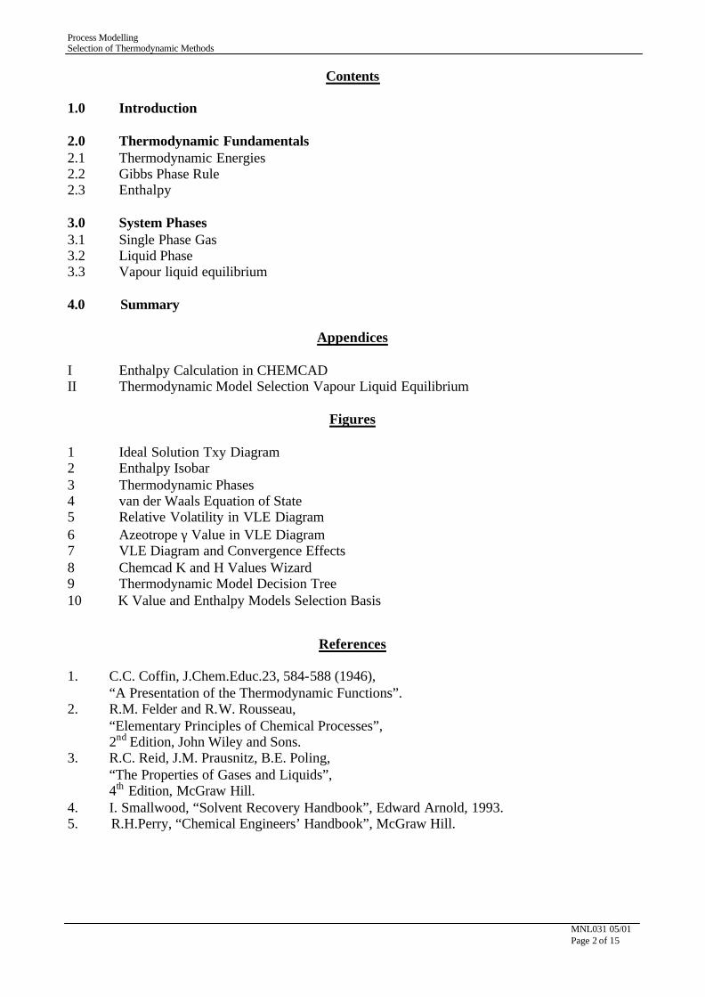
Contents
1.0 Introduction 2.0 Thermodynamic Fundamentals 2.1 Thermodynamic Energies 2.2 Gibbs Phase Rule 2.3 Enthalpy 3.0 System Phases 3.1 Single Phase Gas 3.2 Liquid Phase 3.3 Vapour liquid equilibrium 4.0 Summary
Appendices
I Enthalpy Calculation in CHEMCAD II Thermodynamic Model Selection Vapour Liquid Equilibrium
Figures
1 Ideal Solution Txy Diagram 2 Enthalpy Isobar 3 Thermodynamic Phases 4 van der Waals Equation of State 5 Relative Volatility in VLE Diagram 6 Azeotrope γ Value in VLE Diagram 7 VLE Diagram and Convergence Effects 8 Chemcad K and H Values Wizard 9 Thermodynamic Model Decision Tree 10 K Value and Enthalpy Models Selection Basis
References
1. C.C. Coffin, J.Chem.Educ.23, 584-588 (1946), “A Presentation of the Thermodynamic Functions”. 2. R.M. Felder and R.W. Rousseau, “Elementary Principles of Chemical Processes”, 2nd Edition, John Wiley and Sons. 3. R.C. Reid, J.M. Prausnitz, B.E. Poling, “The Properties of Gases and Liquids”, 4th Edition, McGraw Hill. 4. I. Smallwood, “Solvent Recovery Handbook”, Edward Arnold, 1993. 5. R.H.Perry, “Chemical Engineers’ Handbook”, McGraw Hill.
Process Modelling Selection of Thermodynamic Methods
MNL031 05/01 Page 3 of 15
1.0 INTRODUCTION
The selection of a suitable thermodynamic model for the prediction of enthalpy (H) and phase equilibrium (K) is fundamental to process modelling. Selection of an inappropriate model will result in convergence problems and erroneous results. The selection process is driven by considering the following:-
Process species and compositions. Pressure and temperature ranges. Phase systems involved. Nature of the fluids. Availability of data.
There are four categories of thermodynamic models:-
Equations-of-State (E-o-S) Activity coefficient (γ) Empirical Special system specific
This paper is not intended to be a rigorous analysis of the methods available and their selection but is offered as an aide memoire to the practicing engineer who is looking for rapid, realistic results from his process models. The study of complex systems invariably involves extensive research and expenditure of considerable manpower effort by specialists. There are extensive sources of data available from data banks run by DECHEMA, DIPPR and others. This paper presents practical selection methods and suggests techniques to test the validity of the thermodynamic model selected.
Process Modelling Selection of Thermodynamic Methods
MNL031 05/01 Page 4 of 15
2.0 THERMODYNAMIC FUNDAMENTALS 2.1 Thermodynamic Energies(1)
The thermodynamic fundamentals of fluid states in relation to energies and phase behaviour needs to be thoroughly understood. Four thermodynamic variables determine six thermodynamic energies Intensive variables Extensive variables (capacity) Pressure (P) Volume (V) Temperature (T) Entropy (S) We define thermodynamic energy as follows Energy = Intensity variable x Extensive variable P or T V or S TS represents internal bound energy isothermally unavailable. PV represents external free energy. Helmholtz free energy (F) is the internal energy available for work and is part of the internal energy (U) We have the following energy relationships Internal energy FSTU ++==
Gibbs free energy VPFG ++==
Enthalpy VPFSTH ++++==
VPUH ++== When considering chemical reactions we have Chemical energy = chemical potential factor x capacity factor (( ))dndU i
0ii µµ−−µµ==
Where dni is change in species i moles
µµi is chemical potential species i
dndVPdSTdU ii
i∑∑ µµ++−−==
For equilibrium 0dn ii
i ==∑∑ µµ
Other equilibrium conditions (( ))T&constV0dF == (( ))T&constP0dG ==
(( ))V&constS0dU == (( ))P&constS0dH == It can be shown that nG i
ii∑∑ µµ==
Process Modelling Selection of Thermodynamic Methods
MNL031 05/01 Page 5 of 15
2.2 Gibbs Phase Rule(2)
The variables that define a process condition are in two categories Extensive variables moles, mass, volume Intensive variables temperature, pressure, density, specific volume, mass and mole fractions of components i. The number of intensive variables that can be independently specified for a system at equilibrium is called the number of degrees of freedom F and is given by the Gibbs Phase Rule.In a system involving no reactions this is given by pm2F −−++==
Where m = no of chemical species i p = number of system phases With r independent reactions at equilibrium prm2F −−−−++==
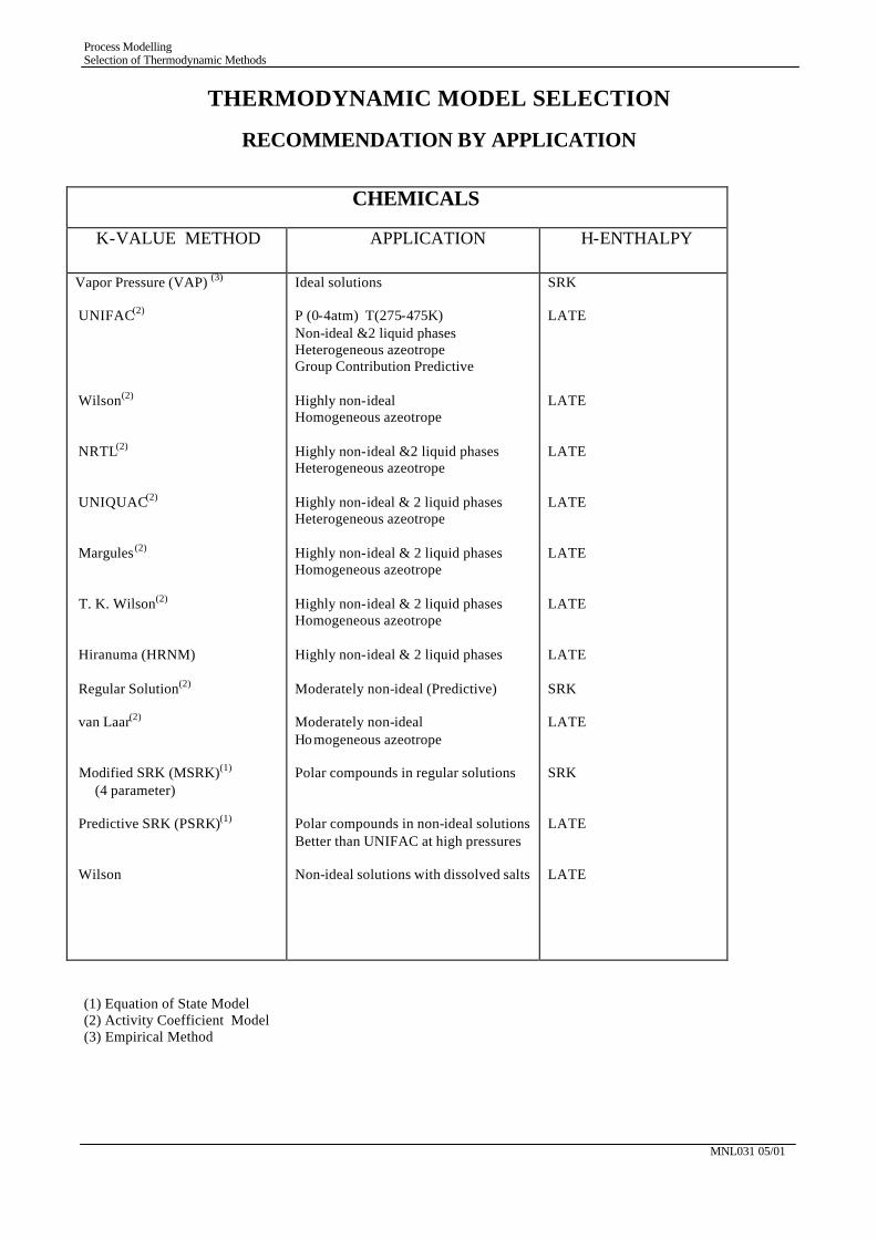
When defining a stream condition in the model the phase rule applies. Consider a single component liquid in equilibrium with its vapour and an inert. Giving m = 2 p = 2 F = 2 Two variables P and T or Vapour fraction (v) with T or P will define the stream. For a binary liquid system one degree of freedom is consumed by the composition leaving either P or T to be specified.In a VLE system it is preferable to specify P which then allows system analysis using Txy plots. When setting up the FlashUnitOp applying the phase rule will ensure that relevant flash conditions are being set. The stream flash calculation can be used to determine the boiling point and dew point of mixtures with and without inerts present by applying the following. The bubble point of a liquid at the given pressure is determined by a flash calculation at a vapour fraction of 0. The dew point of a vapour at the given pressure is determined by a flash calculation at a vapour fraction of 1. For a pure component the bubble point and the dew point are identical so a flash calculation at a vapour fraction of 0 or 1 will yield the same result Figure 1 shows the Txy diagram for Benzene/Toluene,a near ideal mixture.The bubble point for a given composition is read directly from the liquid curve and the dew point is read directly from the vapour curve.
Process Modelling Selection of Thermodynamic Methods
MNL031 05/01 Page 6 of 15
2.3 Enthalpy
Enthalpy is the sum of the internal energy (U) and the external free energy (PV) VPUH ++== The heat supplied is given by
dVPdUdQ ++== The sign convention should be noted and is + for heat added and dU gain in internal energy dTCdU v== The specific heat at constant pressure Cp is related to heat input dTCdQ p==
The adiabatic index or specific ratio γ is defined
C
C
v
p==γγ
It can be shown that the following relationship holds
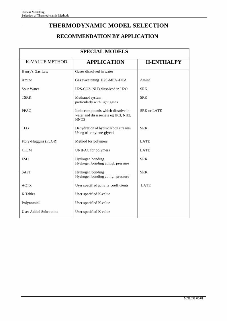
RCC vp ==−− The heating of a liquid at constant pressure e.g. water is considered in Figure 2 This shows the relationships between the enthalpies in the different phases namely the sensible heat in the liquid phase, the latent heat of vaporisation during the vapour liquid equilibrium phase and the superheat in the gas phase. Enthalpy is calculated using Latent Heat (LATE) in the liquid and vle phases and E-o-S (SRK) in the superheated or gas phase. Appendix I reviews the calculation methods adopted in CHEMCAD. A standard reference state of 298ºK for the liquid heat of formation is used providing the advantage that the pressure has no influence on the liquid Cp The enthalpy method used will depend on the K-value method selected as detailed in Appendix II with the following exceptions
Peng Robinson (PR) H value PR Benedict-Webb-Ruben-Starling (BWRS) H value BWRS Grayson Streed (GS) and ESSO H value Lee Kessler Amine H value Amine
Special methods are used for Enthalpy of water steam tables (empirical) Acid gas absorption by DEA and MEA Solid components
Process Modelling Selection of Thermodynamic Methods
MNL031 05/01 Page 7 of 15
3.0 SYSTEM PHASES
There are three phase states namely solid, liquid and gas. Processes comprise either single phase or multiphase systems with separation processes involving at least two phases. Processes involving solids such as filtration and crystallisation, solid – liquid systems and drying, solid – gas system are special cases and receive no further consideration here. The primary area of interest for thermodynamic model selection involve two phases. Liquid – liquid systems, such as extraction and extractive distillation, where liquid – liquid equilibrium (LLE) is considered and vapour liquid systems, such as distillation, stripping and absorption, where vapour – liquid equilibrium (VLE) is considered. Figure 3 shows the inter-relationships between the sys tem phases for a series of isotherms based on the E-o-S due to van-der-Waal. This figure provides the first indication of the validity of making a thermodynamic model selection for the K-value on the basis of the system phases namely single phase gas by E-o-S and VLE by activity coefficient.
3.1 Single Phase Gas(2)
An E-o-S relates the quantity and volume of gas to the temperature and pressure. The ideal gas law is the simplest E-o-S
TRnVP ==
Where P = absolute pressure of gas V = volume or volume of rate of flow n = number of moles or molar flowrate R = gas constant in consistent units T = absolute temperature In an ideal gas mixture the individual components and the mixture as a whole behave in an ideal manner which yields for component i the following relationships TRnVP ii ==
yn
n
P
pi
ii ==== where yi is mole fraction of i in gas
Pyp ii ==
Ppi
i ==∑∑ where P is the total system pressure
plnTR i0ii ++µµ==µµ
Note that when pi = 1 we have µµ==µµ 0ii the reference condition
As the system temperature decreases and the pressure increases deviations from the ideal gas E-o-S result. There are many equation of state (3) available for predicting non- ideal gas behaviour and another method incorporates a compressibility factor into the ideal gas law.
Process Modelling Selection of Thermodynamic Methods
MNL031 05/01 Page 8 of 15
3.1 Single Phase Gas (Cont.) To predict real gases behaviour the concept of fugacity f is introduced giving flnTR i
0ii ++µµ==µµ
All gases tend to ideal behaviour at low pressures where f ≅≅ p Fugacity is of importance when considering processes exhibiting highly non-ideal behaviour
involving vapour liquid equilibrium. Virial Equation of State is given by the following
(( )) (( ))
++++++==V
TC
V
TB1
TR
VP2
Where B(T) is the second virial coefficient C(T) is the third virial coefficient Note if B = C = 0 the equation reduces to the ideal gas law. Benedict–Webb–Rubin (BWR) Equation of State This E-o-S is in the same form as the above equation extended to a fifth virial coefficient. BWR is accurate for gases containing a single species or a gas mixture with a dominant component eg natural gas, and provides considerable precision. Cubic Equations of State This represents an E-o-S linear in pressure and cubic in volume and is equivalent to the virial equation truncated at the third virial coefficient. One of the first E-o-S was that due to van der Waals (University of Leiden),developed in 1873, which is shown in Figure 4.This was based on two effects 1 The volume of the molecules reduces the amount of free volume in the fluid (V-b) 2 Molecular attraction produces additional pressure.The fluid pressure is corrected by a term related to the attraction parameter a of the molecules (P+a/V2) The resulting equation is
(( )) V
a
bV
TRP 2
−−−−
==
It can be shown from relationship (( ))dp
flndTRV == that for van der Waals equation
(( )) (( )) VTR
a2
bV
b
bV
TRlnfln −−
−−++
−−==
Process Modelling Selection of Thermodynamic Methods
MNL031 05/01 Page 9 of 15
3.1 Single Phase Gas (Cont.) The most widely used cubic E-o-S is the Soave modifications of Redlich-Kwong (SRK) equation which is a modification to van der Waals original equation.
(( )) (( ))bVV
a
bV
TRP ++
αα−−−−
==
Where á, a and b are system parameters. Parameters a and b are determined from the critical temperature Tc and critical Pressure Pc Parameter á is determined from a correlation based on experimental data which uses a constant called the Pitzer acentric factor. (3) At the critical point the two phases (gas and liquid) have exactly the same density (technically one phase). If T > Tc no phase change occurs.
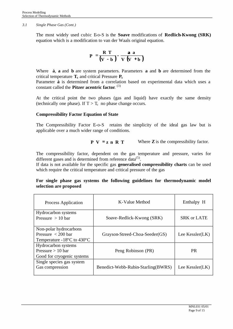
Compressibility Factor Equation of State The Compressibility Factor E-o-S retains the simplicity of the ideal gas law but is applicable over a much wider range of conditions. TRnzVP == Where Z is the compressibility factor. The compressibility factor, dependent on the gas temperature and pressure, varies for different gases and is determined from reference data(5). If data is not available for the specific gas generalised compressibility charts can be used which require the critical temperature and critical pressure of the gas For single phase gas systems the following guidelines for thermodynamic model selection are proposed
Process Application
K-Value Method Enthalpy H
Hydrocarbon systems Pressure > 10 bar
Soave-Redlick-Kwong (SRK) SRK or LATE
Non-polar hydrocarbons Pressure < 200 bar Temperature -18ºC to 430ºC
Grayson-Streed-Choa-Seeder(GS) Lee Kessler(LK)
Hydrocarbon systems Pressure > 10 bar Good for cryogenic systems
Peng Robinson (PR) PR
Single species gas system Gas compression
Benedict-Webb-Rubin-Starling(BWRS) Lee Kessler(LK)
Process Modelling Selection of Thermodynamic Methods
MNL031 05/01 Page 10 of 15
3.2 Liquid Phase
On systems involving liquid phases thermodynamic K-value selection is driven by the nature of the solution. Appendix II provides a summary of thermodynamic selection criteria considered in this section. The following five categories are considered Ideal solution These solutions are non-polar and typically involve hydrocarbons in the same homologous series. Non-ideal solution – regular These solutions exhibit mildly non ideal behaviour and are usually non-polar in nature. Polar solutions – non electrolyte These exhibit highly non-ideal behaviour and will use activity coefficient or special K-value models. Polar solutions – electrolyte Electrolytes are not considered in detail here. However, it should be noted that in modelling they can be treated as true species (molecules and ions) or apparent species (molecules only) There are two methods MNRTL uses K-value NRTL H LATE Pitzer method has no restrictions Binary interaction parameters (BIPs) are required by both methods for accurate modelling. Special Special models have been developed for specific systems. In non-polar applications, such as hydrocarbon processing and refining, due to the complex nature of the mixtures and the large number of species pseudo components are created based on average boiling point, specific gravity and molecular weight. The alternative is to specify all species by molecular formula i.e. real components.
Process Modelling Selection of Thermodynamic Methods
MNL031 05/01 Page 11 of 15
3.2 Liquid Phase Gas (Cont.) Ideal Solutions (3)
In an ideal solution the chemical potential ìi for species i is of the form (( ))xlnTR i
0ii ++µµ==µµ
where µµ0
i is the chemical potential of pure component i If an ideal solution is considered in equilibrium with a perfect gas the phase rule demonstrates that the two phases at a given T and P are not independent. Raoult’s Law describes the distribution of species i between the gas and the liquid phases
pxPyp 0iiii ==== at temperature T
Raoult’s Law is valid when xi is close to 1 as in the case of a single component liquid and over the entire composition range for mixtures with components of similar molecular structure, size and chemical nature. The members of homologous series tend to form ideal mixtures in which the activity coefficient γγ is close to 1 throughout the concentration range. The following systems can be considered suitable for Raoult’s Law. 1 Aliphatic hydrocarbons
Paraffins CnH2n+2 n-hexane (C6H14) n-heptane (C7H16) Olefines CnH2n Alcohols CnH2n+1 •OH methanol (CH3•OH) ethanol (C2H5•OH)
2 Aromatic hydrocarbons benzene (C6H6) toluene (C6H5•CH3)
For ideal liquid systems the following guidelines for thermodynamic model selection are proposed
K – Value Enthalpy
Ideal Vapour Pressure(VAP) SRK
In dilute solutions when xi is close to 0 and with no dissociation, ionisation or reaction in the liquid phase Henry’s law applies where HxPyp iiii ==== at temperature T Henry’s law constants Hi for species i in given solvents are available. Typical applications include slightly soluble gases in aqueous systems.
Process Modelling Selection of Thermodynamic Methods
MNL031 05/01 Page 12 of 15
3.2 Liquid Phase (Cont.) Non-ideal solutions (3)
In a non ideal solution the chemical potential ìi for species i is of the form:- (( ))xlnTR i i
0ii γγ++µµ==µµ
Where γγi is the activity coefficient and component activity xa iii γγ== Consider a non ideal solution in equilibrium with a perfect gas we can derive an equation of the form xkp iiii γγ==
Raoult’s law when γγ i→→1 and xi→→1 pk0ii == giving 1
xp
p
i0i
ii ====γγ
Henry’s law when γγ i→→1 and xi→→ 0 giving Hk ii == For vapour liquid equilibrium at temperature T and pressure P the condition of thermodynamic equilibrium for every component i in a mixture is given by ff l ivi ==
Where the fugacity coefficient Py
f
i
vii ==φφ note 1i ==φφ for ideal gases
The fugacity of component i in the liquid phase is related to the composition of that phase by the activity coefficient γγ as follows
fx
f
x
a0ii
li
i
ii ====γγ
The standard state fugacity f 0
i is at some arbitrarily chosen P and T and in non electrolyte systems is the fugacity of the pure component at system T and P
Process Modelling Selection of Thermodynamic Methods
MNL031 05/01 Page 13 of 15
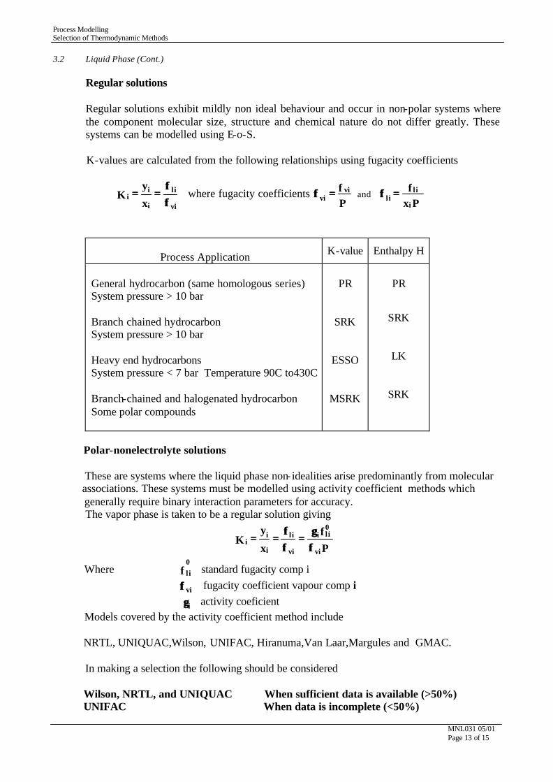
3.2 Liquid Phase (Cont.) Regular solutions Regular solutions exhibit mildly non ideal behaviour and occur in non-polar systems where the component molecular size, structure and chemical nature do not differ greatly. These systems can be modelled using E-o-S.
K-values are calculated from the following relationships using fugacity coefficients
φφφφ
====vi
li
i
ii
x
yK where fugacity coefficients
P
f vivi ==φφ and
Px
f
i
l il i ==φφ
Process Application K-value Enthalpy H
General hydrocarbon (same homologous series) System pressure > 10 bar Branch chained hydrocarbon System pressure > 10 bar Heavy end hydrocarbons System pressure < 7 bar Temperature 90C to430C Branch-chained and halogenated hydrocarbon Some polar compounds
PR
SRK
ESSO
MSRK
PR
SRK
LK
SRK
Polar-nonelectrolyte solutions These are systems where the liquid phase non- idealities arise predominantly from molecular associations. These systems must be modelled using activity coefficient methods which generally require binary interaction parameters for accuracy. The vapor phase is taken to be a regular solution giving
P
f
x
yK
vi
0lii
vi
li
i
ii φφ
γγ==
φφφφ
====
Where f0
li standard fugacity comp i φφvi fugacity coefficient vapour comp i γγi activity coeficient Models covered by the activity coefficient method include NRTL, UNIQUAC,Wilson, UNIFAC, Hiranuma,Van Laar,Margules and GMAC. In making a selection the following should be considered Wilson, NRTL, and UNIQUAC When sufficient data is available (>50%) UNIFAC When data is incomplete (<50%)
Process Modelling Selection of Thermodynamic Methods
MNL031 05/01 Page 14 of 15
3.3 Vapour Liquid Equilibrium(4)
VLE diagrams provide a very useful source of information in relation to the suitability of the K-value selected and the problems presented for the proposed separation. Having selected a K-value method test the Txy and VLE diagrams against known data for the pure components and azeotropes if present. Figure 5 in the attachments shows the VLE diagrams for N-Hexane systems. N-Hexane(1)/N-Heptane(2) can be considered close to representing ideal behaviour which is indicated by the curve symmetry (γ ≅ 1).The different binary systems presented in Figure 5 demonstrate the effect of an increasing α and its influence on ease of separation. We can investigate the effect of γ on α by considering the following
pxp01111 γγ== and pxp
02222 γγ==
γγγγ
αα==γγ
γγ==αα2
10022
011
p
p where αα 0 is the ideal mixture value
Since γ > 1 is the usual situation,except in molecules of a very diferent size, the actual relative volatility is very often much less than the ideal relative volatility particularly at the column top. Values of γ can be calculated throughout the concentration range using van Laar’s equation
++==γγ
xAxA1
1Aln
221
112
2
121 where γγ== ∞∞112 lnA with ∞∞ representing infinite dilution
An extensive data bank providing values of parameter Axy are available from Dechema. Values of γ can also be calculated at an azeotrope which can be very useful due to the extensive azeotropic data available in the literature.
At an azeotrope we have yx 11 == giving pxPy 01111 γγ== resulting in
p
P01
1 ==γγ
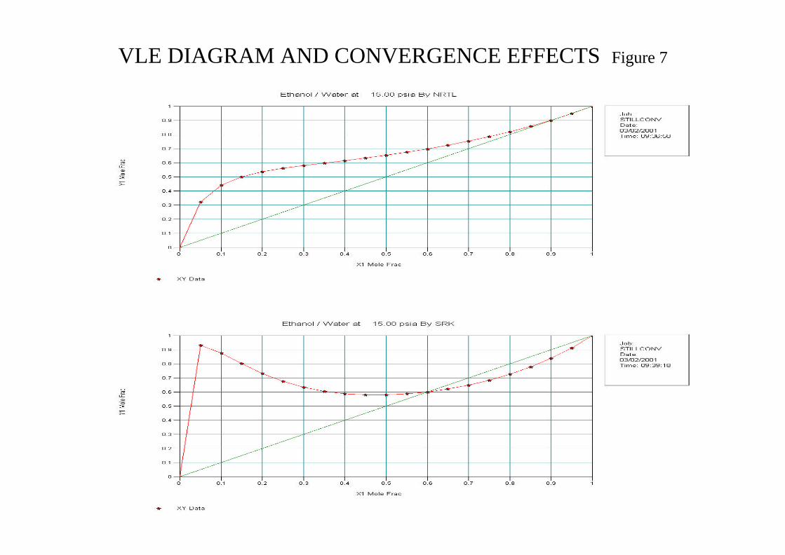
Figure 6 in the attachments shows the VLE diagrams for N-Hexane(1)/Ethyl Acetate(2) system. CHEMCAD Wizard selected K-value NRTL and H Latent Heat and it can be seen that the model is reasonably accurate against known data.The γ values are shown and the ir influence seen at the column bottom and top. Figure 7 in the attachments shows the VLE diagrams for Ethanol(1)/Water(2) using K-value method NRTL and SRK which clearly demonstrates the importance of model selection.To achieve convergence for high purity near the azeotropic composition it is recommended to start the simulation with “slack” parameters which can be loaded as initial column profile(set flag) and then tighten the specification iteratively.
Process Modelling Selection of Thermodynamic Methods
MNL031 05/01 Page 15 of 15
4.0 Summary
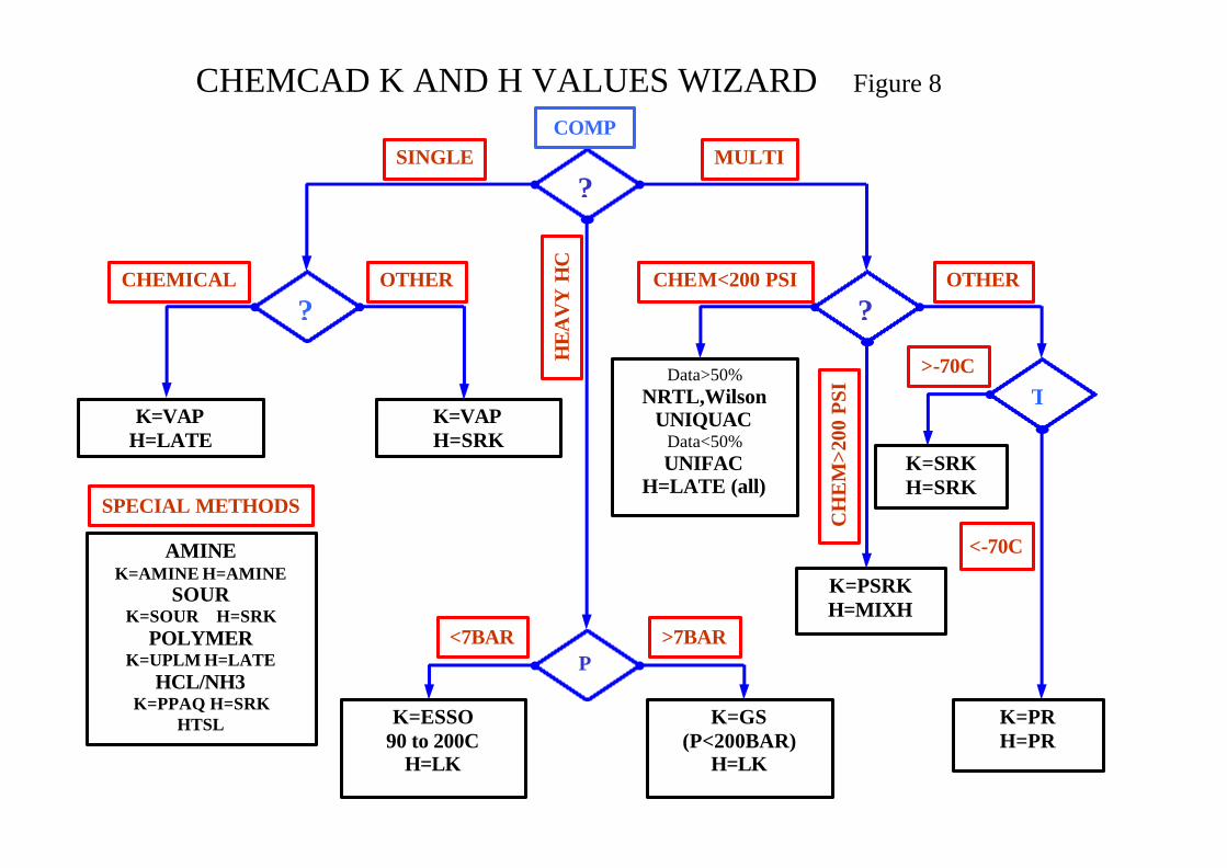
CHEMCAD provides a K-Value Wizard as an aide to thermodynamic model selection. The selection is essentially based on the component list and operating temperature and pressure ranges.The Wizard decides which model to use between E-o-S,activity coefficient,empirical and special.If inadequate BIP data is available for the activity coefficient method the Wizard defaults toUNIFAC. The key decision paths in the method are shown in Figure 8 in the attachments. If using the Wizard exclude utility streams from the component list as the presence of water for example will probably lead to an incorrect selection. The following additional points should to be considered when setting the K-Value Vapour phase association typical systems acetic acid, formic acid, acrylic acid Vapour fugacity correction set when using an activity coefficient method P>1bar Water/hydrocarbon solubility immiscibility valid only for non activity coefficient
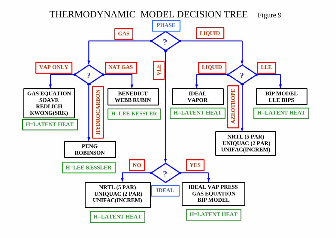
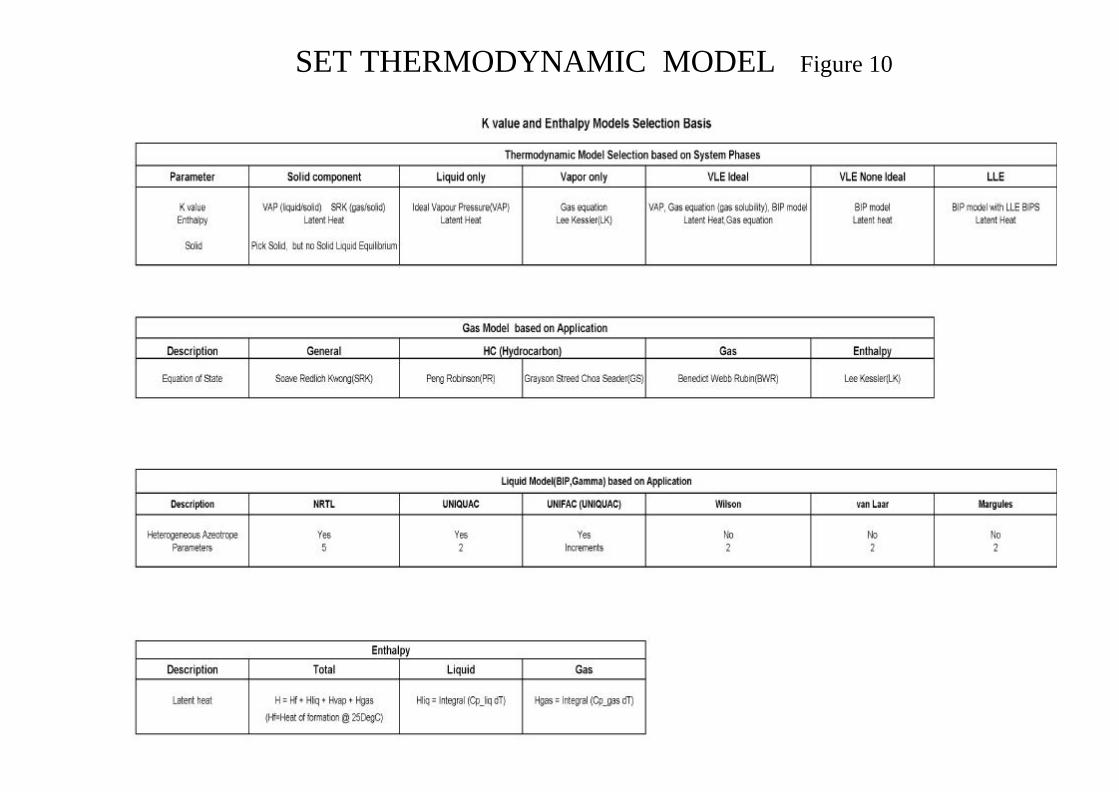
methods for which water is assumed to be miscible Salt considers effect of dissolved salts when using the Wilson method In the attachments can be found summary tables providing a basis for model selection. A thermodynamic model decision tree based on system phases is shown in Figure 9. A synopsis on Thermodynamic Model Selection is presented in Appendix II
Process Modelling Selection of Thermodynamic Methods
MNL031 05/01
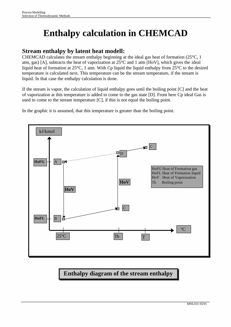
Enthalpy calculation in CHEMCAD Stream enthalpy by latent heat modell: CHEMCAD calculates the stream enthalpy beginning at the ideal gas heat of formation (25°C, 1 atm, gas) [A], subtracts the heat of vaporization at 25°C and 1 atm [HoV], which gives the ideal liquid heat of formation at 25°C, 1 atm. With Cp liquid the liquid enthalpy from 25°C to the desired temperature is calculated next. This temperature can be the stream temperature, if the stream is liquid. In that case the enthalpy calculation is done. If the stream is vapor, the calculation of liquid enthalpy goes until the boiling point [C] and the heat of vaporization at this temperature is added to come to the gas state [D]. From here Cp ideal Gas is used to come to the stream temperature [C], if this is not equal the boiling point. In the graphic it is assumed, that this temperature is greater than the boiling point.
Enthalpy diagram of the stream enthalpy
kJ/kmol
°C
25°C Tb T
HoFG
HoFL
A
B
C
D
C
HoV
HoV
HoFG Heat of Formation gas HoFL Heat of Formation liquid HoV Heat of Vaporozation Tb Boiling point
Process Modelling Selection of Thermodynamic Methods
MNL031 05/01
Using the liquid heat of formation as a starting point instead of the gas heat of formation has the advantage, that the pressure has no influence to Cp liquid. If the stream is liquid that should be the best way. If the stream is gas there will be still a small problem if the stream pressure is high, because Cp gas is measured for ideal gas only and there is no pressure correction available.
Stream enthalpy by equation of state modell: The gas enthalpy can also be calculated using the equation of state. CHEMCAD begins in that case with the ideal gas heat of formation. This has the advantage for the gas phase that the pressure is part of the enthalpy. The gas models are SRK, PR, Lee Kessler etc. In the liquid phase these models are not so good as the Cp liquid calculation using the latent heat model. In the case the liquid is highly non ideal the user should select the latent heat model and not an equation of state for enthalpy calculation. This is the reason why the thermodynamic expert selects NRTL, or UNIQUAC or UNIFAC together only with latent heat as the best enthalpy model
A check: Calculating the stream enthalpy at 25°C, 1 atm which means the user goes from A to B to C to D to A. this should give the ideal gas heat of formation at 25°C, 1 atm. Theoretically the thermodynamic rules says that, but because of errors in the measured physical properties, which are used here, there will be a small deviation in comparison to the data of the databank if the modell is latent heat.
A good decision: A great number of systems where checked until CHEMSTATIONS decided to calculate the stream enthalpy in the described way. However, we are in discussion with our users about enthalpy.
Reactor enthalpy calculation The calculation of enthalpy in the CHEMCAD reactors are discussed now. We will begin with an easy example of a gas reaction. This is the gas reaction which we will investigate first:
Process Modelling Selection of Thermodynamic Methods
MNL031 05/01
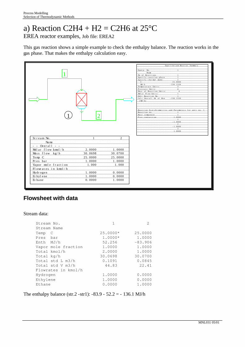
a) Reaction C2H4 + H2 = C2H6 at 25°C EREA reactor examples, Job file: EREA2 This gas reaction shows a simple example to check the enthalpy balance. The reaction works in the gas phase. That makes the enthalpy calculation easy.
Flowsheet with data Stream data: Stream No. 1 2 Stream Name Temp C 25.0000* 25.0000 Pres bar 1.0000* 1.0000 Enth MJ/h 52.256 -83.906 Vapor mole fraction 1.0000 1.0000 Total kmol/h 2.0000 1.0000 Total kg/h 30.0698 30.0700 Total std L m3/h 0.1091 0.0845 Total std V m3/h 44.83 22.41 Flowrates in kmol/h Hydrogen 1.0000 0.0000 Ethylene 1.0000 0.0000 Ethane 0.0000 1.0000 The enthalpy balance (str.2 -str1): -83.9 - 52.2 = - 136.1 MJ/h
1
1
2
Stream No. 1 2
Name- - Overall - -Molar flow kmol/h 2.0000 1.0000Mass flow kg/h 30.0698 30.0700
Temp C 25.0000 25.0000Pres bar 1.0000 1.0000Vapor mole fraction 1.000 1.000
Flowrates in kmol/hHydrogen 1.0000 0.0000Ethylene 1.0000 0.0000Ethane 0.0000 1.0000
Equilibrium Reactor Summary
Equip. No. 1
Name
No of Reactions 1 Specify reaction phase 1
Specify thermal mode: 2 C 25.0000
MJ/h -136.1326Temperature Units: 3
Pressure Units: 4 Heat of Reaction Units: 4
Molar Flow Units: 1
Edit Reaction No. 1 Calc Overall Ht of Rxn -136.1330
(MJ/h)
Reaction Stoichiometrics and Parameters for unit no. 1Reaction no. 1
Base component 1
Frac.conversion 1.0000 1
-1.0000 2
-1.0000 3
1.0000
Process Modelling Selection of Thermodynamic Methods
MNL031 05/01
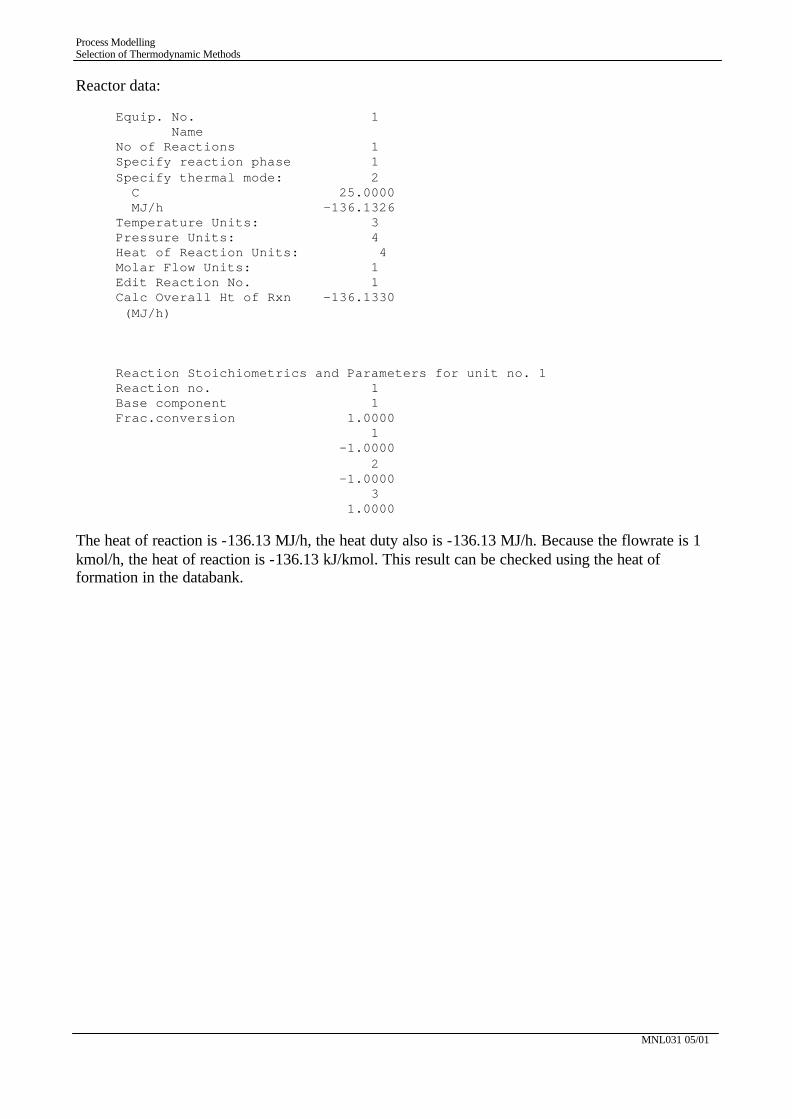
Reactor data: Equip. No. 1 Name No of Reactions 1 Specify reaction phase 1 Specify thermal mode: 2 C 25.0000 MJ/h -136.1326 Temperature Units: 3 Pressure Units: 4 Heat of Reaction Units: 4 Molar Flow Units: 1 Edit Reaction No. 1 Calc Overall Ht of Rxn -136.1330 (MJ/h) Reaction Stoichiometrics and Parameters for unit no. 1 Reaction no. 1 Base component 1 Frac.conversion 1.0000 1 -1.0000 2 -1.0000 3 1.0000 The heat of reaction is -136.13 MJ/h, the heat duty also is -136.13 MJ/h. Because the flowrate is 1 kmol/h, the heat of reaction is -136.13 kJ/kmol. This result can be checked using the heat of formation in the databank.
Process Modelling Selection of Thermodynamic Methods
MNL031 05/01
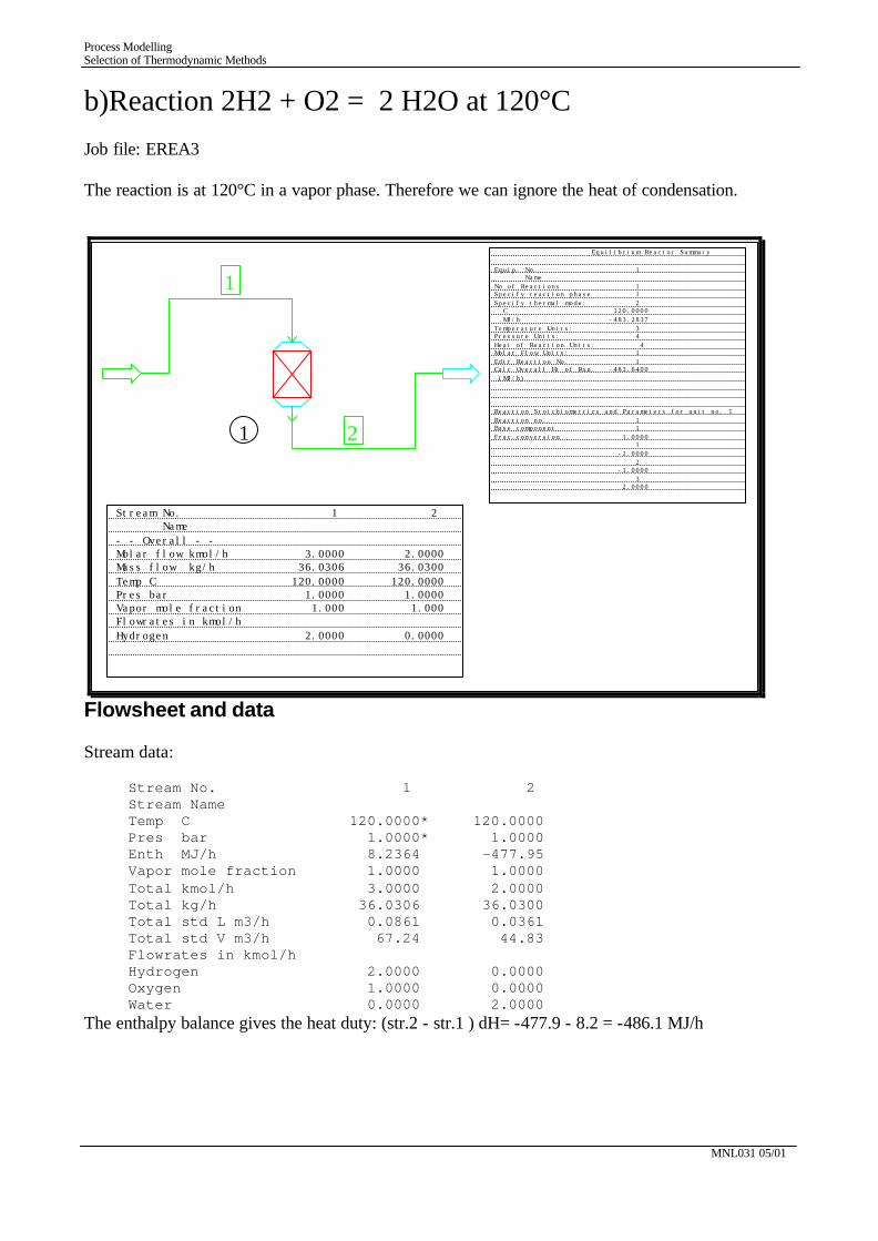
b)Reaction 2H2 + O2 = 2 H2O at 120°C Job file: EREA3 The reaction is at 120°C in a vapor phase. Therefore we can ignore the heat of condensation.
Flowsheet and data Stream data: Stream No. 1 2 Stream Name Temp C 120.0000* 120.0000 Pres bar 1.0000* 1.0000 Enth MJ/h 8.2364 -477.95 Vapor mole fraction 1.0000 1.0000 Total kmol/h 3.0000 2.0000 Total kg/h 36.0306 36.0300 Total std L m3/h 0.0861 0.0361 Total std V m3/h 67.24 44.83 Flowrates in kmol/h Hydrogen 2.0000 0.0000 Oxygen 1.0000 0.0000 Water 0.0000 2.0000 The enthalpy balance gives the heat duty: (str.2 - str.1 ) dH= -477.9 - 8.2 = -486.1 MJ/h
1
1
2
Stream No. 1 2 Name
- - Overall - -Molar flow kmol/h 3.0000 2.0000Mass flow kg/h 36.0306 36.0300
Temp C 120.0000 120.0000Pres bar 1.0000 1.0000Vapor mole fraction 1.000 1.000Flowrates in kmol/h
Hydrogen 2.0000 0.0000��
Equilibrium Reactor Summary
Equip. No. 1 Name
No of Reactions 1 Specify reaction phase 1
Specify thermal mode: 2 C 120.0000
MJ/h -483.2837
Temperature Units: 3 Pressure Units: 4
Heat of Reaction Units: 4 Molar Flow Units: 1
Edit Reaction No. 1 Calc Overall Ht of Rxn -483.6400
(MJ/h)
Reaction Stoichiometrics and Parameters for unit no. 1
Reaction no. 1Base component 1
Frac.conversion 1.0000 1
-2.0000
2 -1.0000
3 2.0000
Process Modelling Selection of Thermodynamic Methods
MNL031 05/01
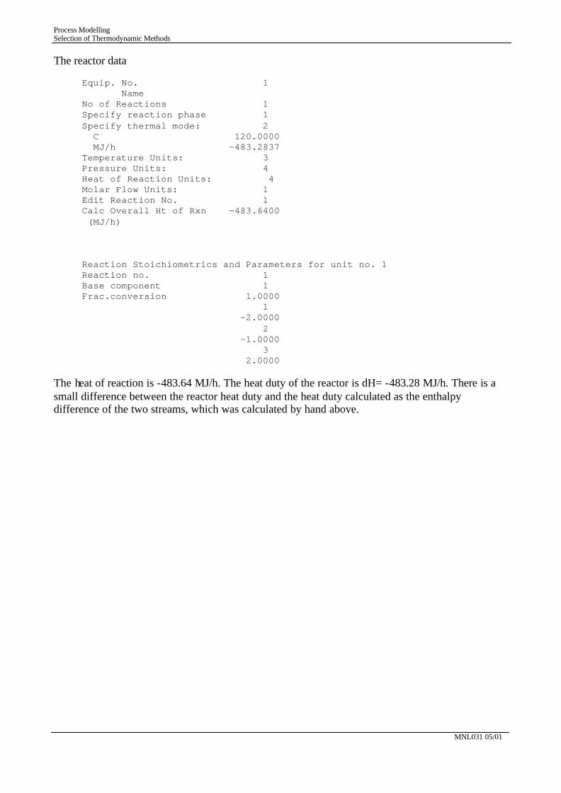
The reactor data Equip. No. 1 Name No of Reactions 1 Specify reaction phase 1 Specify thermal mode: 2 C 120.0000 MJ/h -483.2837 Temperature Units: 3 Pressure Units: 4 Heat of Reaction Units: 4 Molar Flow Units: 1 Edit Reaction No. 1 Calc Overall Ht of Rxn -483.6400 (MJ/h) Reaction Stoichiometrics and Parameters for unit no. 1 Reaction no. 1 Base component 1 Frac.conversion 1.0000 1 -2.0000 2 -1.0000 3 2.0000 The heat of reaction is -483.64 MJ/h. The heat duty of the reactor is dH= -483.28 MJ/h. There is a small difference between the reactor heat duty and the heat duty calculated as the enthalpy difference of the two streams, which was calculated by hand above.
Process Modelling Selection of Thermodynamic Methods
MNL031 05/01
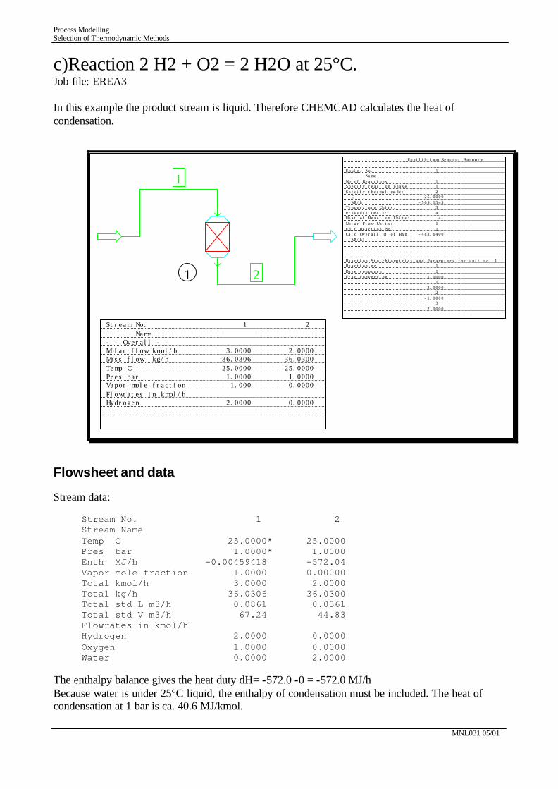
c)Reaction 2 H2 + O2 = 2 H2O at 25°C. Job file: EREA3 In this example the product stream is liquid. Therefore CHEMCAD calculates the heat of condensation.
Flowsheet and data Stream data: Stream No. 1 2 Stream Name Temp C 25.0000* 25.0000 Pres bar 1.0000* 1.0000 Enth MJ/h -0.00459418 -572.04 Vapor mole fraction 1.0000 0.00000 Total kmol/h 3.0000 2.0000 Total kg/h 36.0306 36.0300 Total std L m3/h 0.0861 0.0361 Total std V m3/h 67.24 44.83 Flowrates in kmol/h Hydrogen 2.0000 0.0000 Oxygen 1.0000 0.0000 Water 0.0000 2.0000 The enthalpy balance gives the heat duty dH= -572.0 -0 = -572.0 MJ/h Because water is under 25°C liquid, the enthalpy of condensation must be included. The heat of condensation at 1 bar is ca. 40.6 MJ/kmol.
1
1
2
Stream No. 1 2
Name- - Overall - -Molar flow kmol/h 3.0000 2.0000Mass flow kg/h 36.0306 36.0300
Temp C 25.0000 25.0000Pres bar 1.0000 1.0000Vapor mole fraction 1.000 0.0000
Flowrates in kmol/hHydrogen 2.0000 0.0000��
Equilibrium Reactor Summary
Equip. No. 1 Name
No of Reactions 1 Specify reaction phase 1
Specify thermal mode: 2 C 25.0000
MJ/h -569.1345Temperature Units: 3
Pressure Units: 4 Heat of Reaction Units: 4
Molar Flow Units: 1
Edit Reaction No. 1 Calc Overall Ht of Rxn -483.6400
(MJ/h)
Reaction Stoichiometrics and Parameters for unit no. 1Reaction no. 1
Base component 1
Frac.conversion 1.0000 1
-2.0000 2
-1.0000 3
2.0000
Process Modelling Selection of Thermodynamic Methods
MNL031 05/01
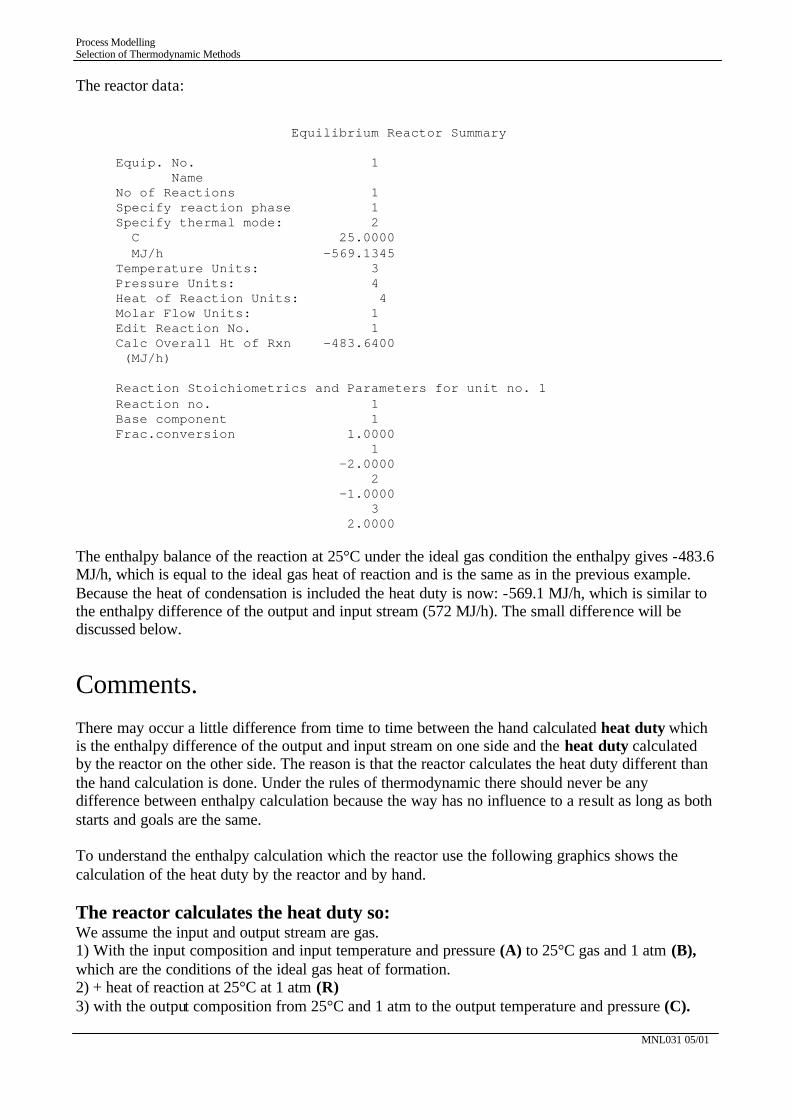
The reactor data: Equilibrium Reactor Summary Equip. No. 1 Name No of Reactions 1 Specify reaction phase 1 Specify thermal mode: 2 C 25.0000 MJ/h -569.1345 Temperature Units: 3 Pressure Units: 4 Heat of Reaction Units: 4 Molar Flow Units: 1 Edit Reaction No. 1 Calc Overall Ht of Rxn -483.6400 (MJ/h) Reaction Stoichiometrics and Parameters for unit no. 1 Reaction no. 1 Base component 1 Frac.conversion 1.0000 1 -2.0000 2 -1.0000 3 2.0000 The enthalpy balance of the reaction at 25°C under the ideal gas condition the enthalpy gives -483.6 MJ/h, which is equal to the ideal gas heat of reaction and is the same as in the previous example. Because the heat of condensation is included the heat duty is now: -569.1 MJ/h, which is similar to the enthalpy difference of the output and input stream (572 MJ/h). The small difference will be discussed below.
Comments. There may occur a little difference from time to time between the hand calculated heat duty which is the enthalpy difference of the output and input stream on one side and the heat duty calculated by the reactor on the other side. The reason is that the reactor calculates the heat duty different than the hand calculation is done. Under the rules of thermodynamic there should never be any difference between enthalpy calculation because the way has no influence to a result as long as both starts and goals are the same. To understand the enthalpy calculation which the reactor use the following graphics shows the calculation of the heat duty by the reactor and by hand. The reactor calculates the heat duty so: We assume the input and output stream are gas. 1) With the input composition and input temperature and pressure (A) to 25°C gas and 1 atm (B), which are the conditions of the ideal gas heat of formation. 2) + heat of reaction at 25°C at 1 atm (R) 3) with the output composition from 25°C and 1 atm to the output temperature and pressure (C).
Process Modelling Selection of Thermodynamic Methods
MNL031 05/01
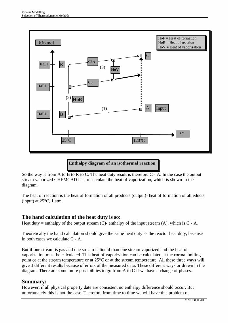
So the way is from A to B to R to C. The heat duty result is therefore C - A. In the case the output stream vaporized CHEMCAD has to calculate the heat of vaporization, which is shown in the diagram. The heat of reaction is the heat of formation of all products (output)- heat of formation of all educts (input) at 25°C, 1 atm. The hand calculation of the heat duty is so: Heat duty = enthalpy of the output stream (C)- enthalpy of the input stream (A), which is C - A. Theoretically the hand calculation should give the same heat duty as the reactor heat duty, because in both cases we calculate C - A. But if one stream is gas and one stream is liquid than one stream vaporized and the heat of vaporization must be calculated. This heat of vaporization can be calculated at the normal boiling point or at the stream temperature or at 25°C or at the stream temperature. All these three ways will give 3 different results because of errors of the measured data. These different ways or drawn in the diagram. There are some more possibilities to go from A to C if we have a change of phases. Summary: However, if all physical property date are consistent no enthalpy difference should occur. But unfortunately this is not the case. Therefore from time to time we will have this problem of
HoF = Heat of formation HoR = Heat of reaction HoV = Heat of vaporization
Enthalpy diagram of an isothermal reaction
kJ/kmol
°C
A
B
25°C 120°C
C
R
HoR
(1)
(3)
(2)
HoFL Input
HoF2
CpL
HoV
CPG
HoFL

Process Modelling Selection of Thermodynamic Methods
MNL031 05/01
enthalpie difference, but it will be small. In that case we will check the data and the way of calculation again. But in any case for the process simulation the way CHEMCAD uses to calculates the enthalpy seems to be the best way of all other ways. This was checked for a great number of cases. In the case physical properties are not available in the databank CHEMCAD has to change the way of calculation to come to a result, which means that the enthalpy difference may occur greater or smaller depending by the selected way. Remark: This problem description is a comment and not an official description of CHEMSTATIONS Inc. USA.
Process Modelling Selection of Thermodynamic Methods
MNL031 05/01
THERMODYNAMIC MODEL SELECTION
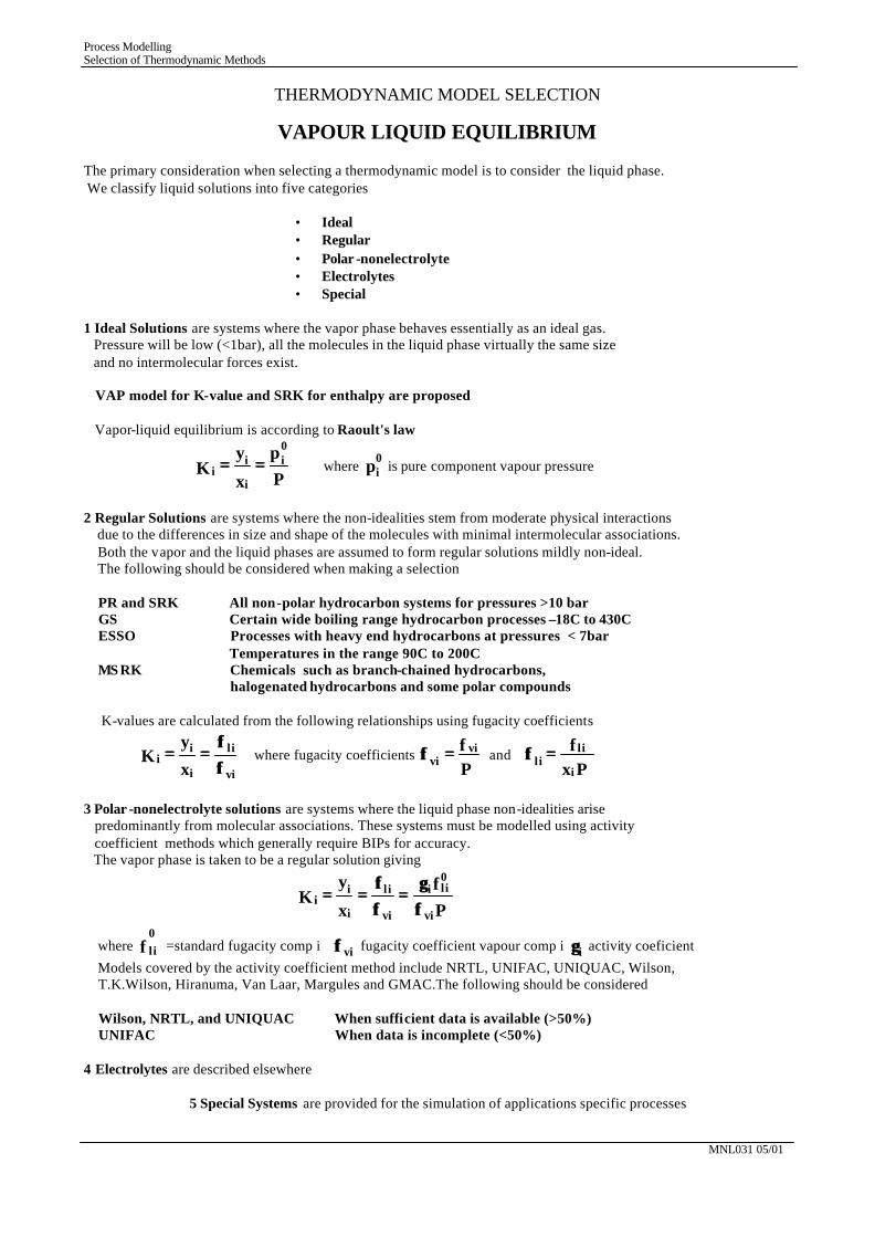
VAPOUR LIQUID EQUILIBRIUM The primary consideration when selecting a thermodynamic model is to consider the liquid phase. We classify liquid solutions into five categories
• Ideal • Regular • Polar -nonelectrolyte • Electrolytes • Special
1 Ideal Solutions are systems where the vapor phase behaves essentially as an ideal gas. Pressure will be low (<1bar), all the molecules in the liquid phase virtually the same size and no intermolecular forces exist. VAP model for K-value and SRK for enthalpy are proposed Vapor-liquid equilibrium is according to Raoult's law
P
p
x
yK
0i
i
ii ==== where p
0i is pure component vapour pressure
2 Regular Solutions are systems where the non-idealities stem from moderate physical interactions due to the differences in size and shape of the molecules with minimal intermolecular associations. Both the vapor and the liquid phases are assumed to form regular solutions mildly non-ideal. The following should be considered when making a selection PR and SRK All non-polar hydrocarbon systems for pressures >10 bar GS Certain wide boiling range hydrocarbon processes –18C to 430C ESSO Processes with heavy end hydrocarbons at pressures < 7bar Temperatures in the range 90C to 200C MS RK Chemicals such as branch-chained hydrocarbons, halogenated hydrocarbons and some polar compounds K-values are calculated from the following relationships using fugacity coefficients
φφφφ
====vi
li
i
ii
x
yK where fugacity coefficients
P
f vivi ==φφ and
Px
f
i
l il i ==φφ
3 Polar -nonelectrolyte solutions are systems where the liquid phase non-idealities arise predominantly from molecular associations. These systems must be modelled using activity coefficient methods which generally require BIPs for accuracy. The vapor phase is taken to be a regular solution giving
P
f
x
yK
vi
0lii
vi
li
i
ii φφ
γγ==
φφφφ
====
where f0
li =standard fugacity comp i φφvi fugacity coefficient vapour comp i γγi activity coeficient
Models covered by the activity coefficient method include NRTL, UNIFAC, UNIQUAC, Wilson, T.K.Wilson, Hiranuma, Van Laar, Margules and GMAC.The following should be considered Wilson, NRTL, and UNIQUAC When sufficient data is available (>50%) UNIFAC When data is incomplete (<50%) 4 Electrolytes are described elsewhere
5 Special Systems are provided for the simulation of applications specific processes
Process Modelling Selection of Thermodynamic Methods
MNL031 05/01
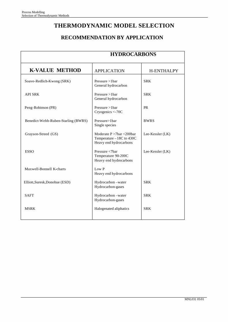
THERMODYNAMIC MODEL SELECTION
RECOMMENDATION BY APPLICATION
HYDROCARBONS
K-VALUE METHOD
APPLICATION
H-ENTHALPY
Soave-Redlich-Kwong (SRK) API SRK Peng-Robinson (PR) Benedict-Webb-Ruben-Starling (BWRS) Grayson-Streed (GS) ESSO Maxwell-Bonnell K-charts Elliott,Suresk,Donohue (ESD) SAFT MSRK
Pressure >1bar General hydrocarbon Pressure >1bar General hydrocarbon Pressure >1bar Cryogenics <-70C Pressure>1bar Single species Moderate P >7bar <200bar Temperature –18C to 430C Heavy end hydrocarbons Pressure <7bar Temperature 90-200C Heavy end hydrocarbons Low P Heavy end hydrocarbons Hydrocarbon –water Hydrocarbon-gases Hydrocarbon –water Hydrocarbon-gases Halogenated aliphatics
SRK SRK PR BWRS Lee-Kessler (LK) Lee-Kessler (LK) SRK SRK SRK
Process Modelling Selection of Thermodynamic Methods
MNL031 05/01
THERMODYNAMIC MODEL SELECTION
RECOMMENDATION BY APPLICATION
CHEMICALS K-VALUE METHOD
APPLICATION
H-ENTHALPY
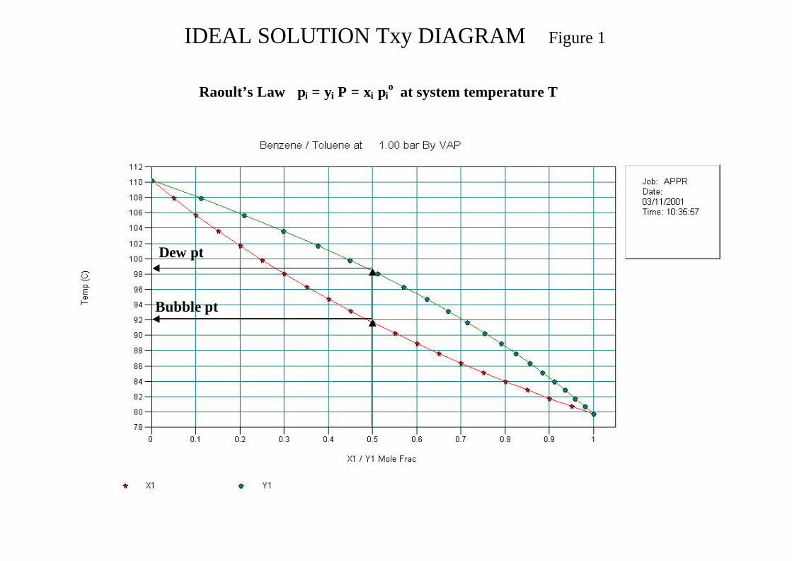
Vapor Pressure (VAP) (3)
UNIFAC(2)
Wilson(2)
NRTL(2)
UNIQUAC(2)
Margules (2)
T. K. Wilson(2)
Hiranuma (HRNM) Regular Solution(2)
van Laar(2)
Modified SRK (MSRK)(1)
(4 parameter)
Predictive SRK (PSRK)(1)
Wilson
Ideal solutions P (0-4atm) T(275-475K) Non-ideal &2 liquid phases Heterogeneous azeotrope Group Contribution Predictive Highly non-ideal Homogeneous azeotrope Highly non-ideal &2 liquid phases Heterogeneous azeotrope Highly non-ideal & 2 liquid phases Heterogeneous azeotrope Highly non-ideal & 2 liquid phases Homogeneous azeotrope Highly non-ideal & 2 liquid phases Homogeneous azeotrope Highly non-ideal & 2 liquid phases Moderately non-ideal (Predictive) Moderately non-ideal Homogeneous azeotrope Polar compounds in regular solutions Polar compounds in non-ideal solutions Better than UNIFAC at high pressures Non-ideal solutions with dissolved salts
SRK LATE LATE LATE LATE LATE LATE LATE SRK LATE SRK LATE LATE
(1) Equation of State Model (2) Activity Coefficient Model (3) Empirical Method
Process Modelling Selection of Thermodynamic Methods
MNL031 05/01
. THERMODYNAMIC MODEL SELECTION
RECOMMENDATION BY APPLICATION
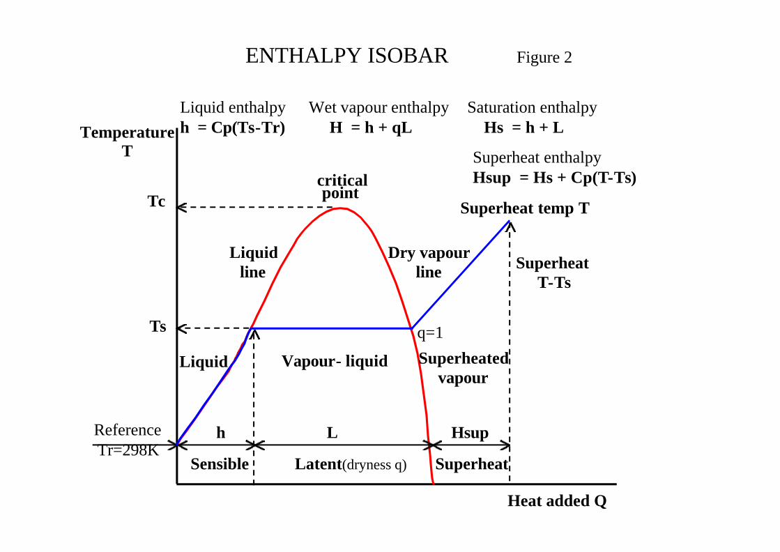
SPECIAL MODELS
K-VALUE METHOD
APPLICATION H-ENTHALPY
Henry's Gas Law
Gases dissolved in water
Amine Gas sweetening H2S-MEA -DEA
Amine
Sour Water
H2S-CO2- NH3 dissolved in H2O SRK
TSRK Methanol system particularly with light gases
SRK
PPAQ Ionic compounds which dissolve in water and disassociate eg HCl, NH3, HNO3
SRK or LATE
TEG Dehydration of hydrocarbon streams Using tri-ethylene-glycol
SRK
Flory-Huggins (FLOR) Method for polymers
LATE
UPLM UNIFAC for polymers
LATE
ESD Hydrogen bonding Hydrogen bonding at high pressure
SRK
SAFT Hydrogen bonding Hydrogen bonding at high pressure
SRK
ACTX User specified activity coefficients
LATE
K Tables
User specified K-value
Polynomial User specified K-value
User-Added Subroutine User specified K-value
IDEAL SOLUTION Txy DIAGRAM Figure 1
Bubble pt
Dew pt
Raoult’s Law pi = yi P = xi pio at system temperature T
ENTHALPY ISOBAR Figure 2
Temperature
T
Heat added Q
critical
Ts
Tc
Vapour- liquid Liquid
point
Dry vapour line
h L
Liquidline
Hsup
Superheat temp T
q=1
Superheatedvapour
Reference Tr=298K
Liquid enthalpy h = Cp(Ts-Tr)
Saturation enthalpy Hs = h + L
Wet vapour enthalpy H = h + qL
Superheat enthalpy Hsup = Hs + Cp(T-Ts)
Sensible Latent(dryness q) Superheat
Superheat T-Ts
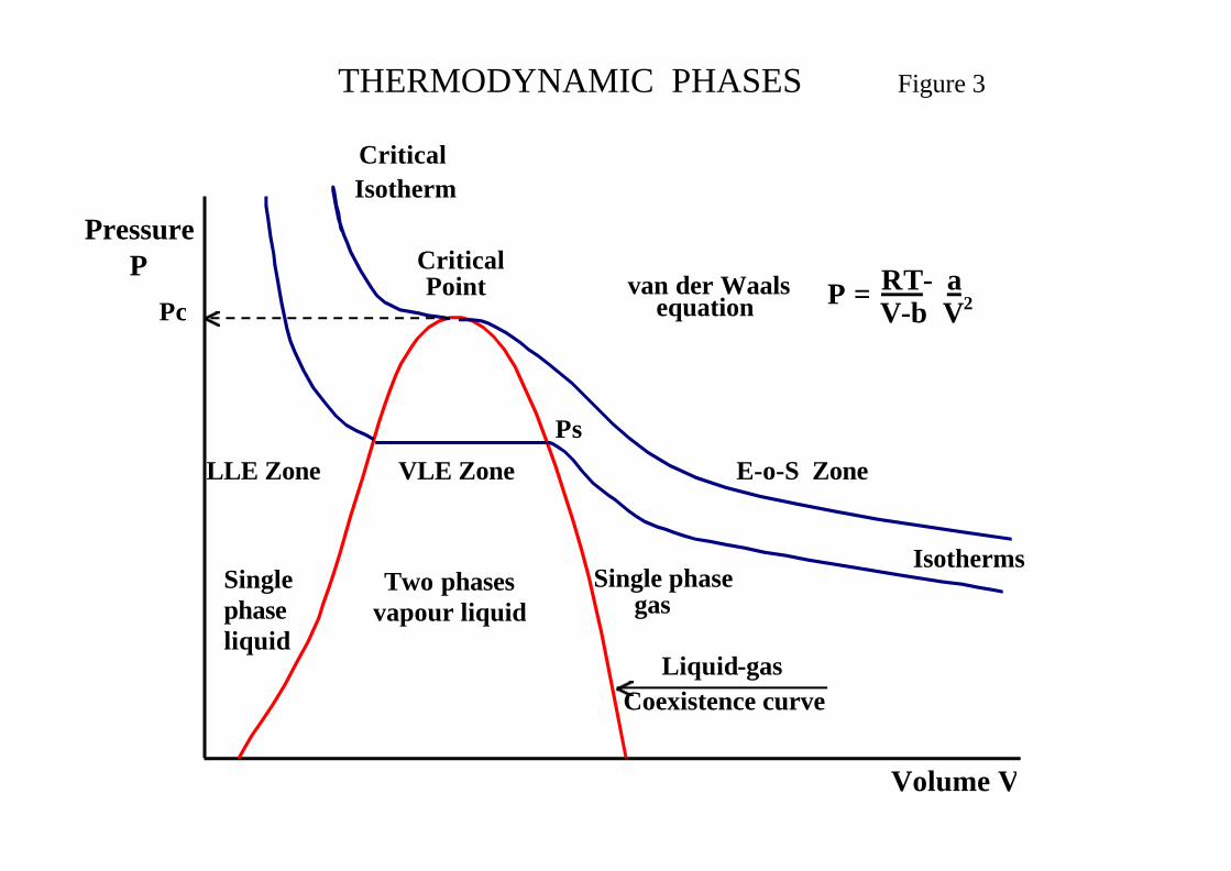
THERMODYNAMIC PHASES Figure 3
Critical
Isotherms
Pressure P
Volume V
Single phase
RT- a V-b V2
van der Waals
Ps
Pc
VLE Zone
Two phases vapour liquid gas
Single phase liquid
LLE Zone
Liquid-gas Coexistence curve
P =equation
E-o-S Zone
Isotherm
Critical Point
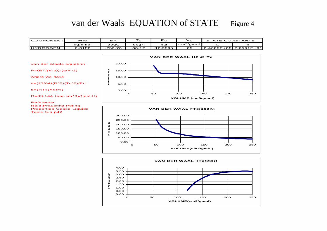
COMPONENT MW BP TC PC VC STATE CONSTANTS
kg/kmol degC degK bar cm3/gmol a bHYDROGEN 2.0158 -252.76 33.12 12.9595 65 2.4685E+05 2.6561E+01
van der Waals equation
P=(RT/(V-b))-(a/V^2)
where we have
a=(27/64)(R^2)(Tc^2)/Pc
b=(RTc)/(8Pc)
R=83.144 (bar.cm^3)/(mol.K)
Reference:Reid,Prausnitz,PolingProperties Gases LiquidsTable 3-5 p42
VAN DER WAAL H2 @ Tc
0.00
5.00
10.00
15.00
20.00
0 50 100 150 200 250
VOLUME (cm3/gmol)
PR
ES
SU
RE
(b
ar)
VAN DER WAAL >Tc(100K)
0.00
50.00
100.00
150.00
200.00
250.00
300.00
0 50 100 150 200 250
VOLUME(cm3/gmol)
PR
ES
SU
RE
(b
ar)
VAN DER WAAL <Tc(20K)
0.00
0.50
1.00
1.50
2.00
2.50
3.00
3.50
4.00
0 50 100 150 200 250
VOLUME(cm3/gmol)
PR
ES
SU
RE
(b
ar)
van der Waals EQUATION of STATE Figure 4
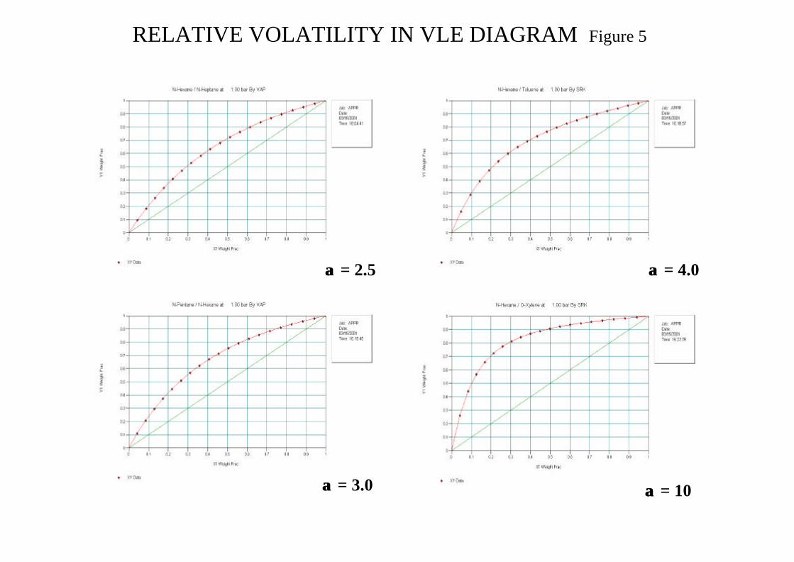
RELATIVE VOLATILITY IN VLE DIAGRAM Figure 5
αα = 2.5
αα = 10
αα = 4.0
αα = 3.0
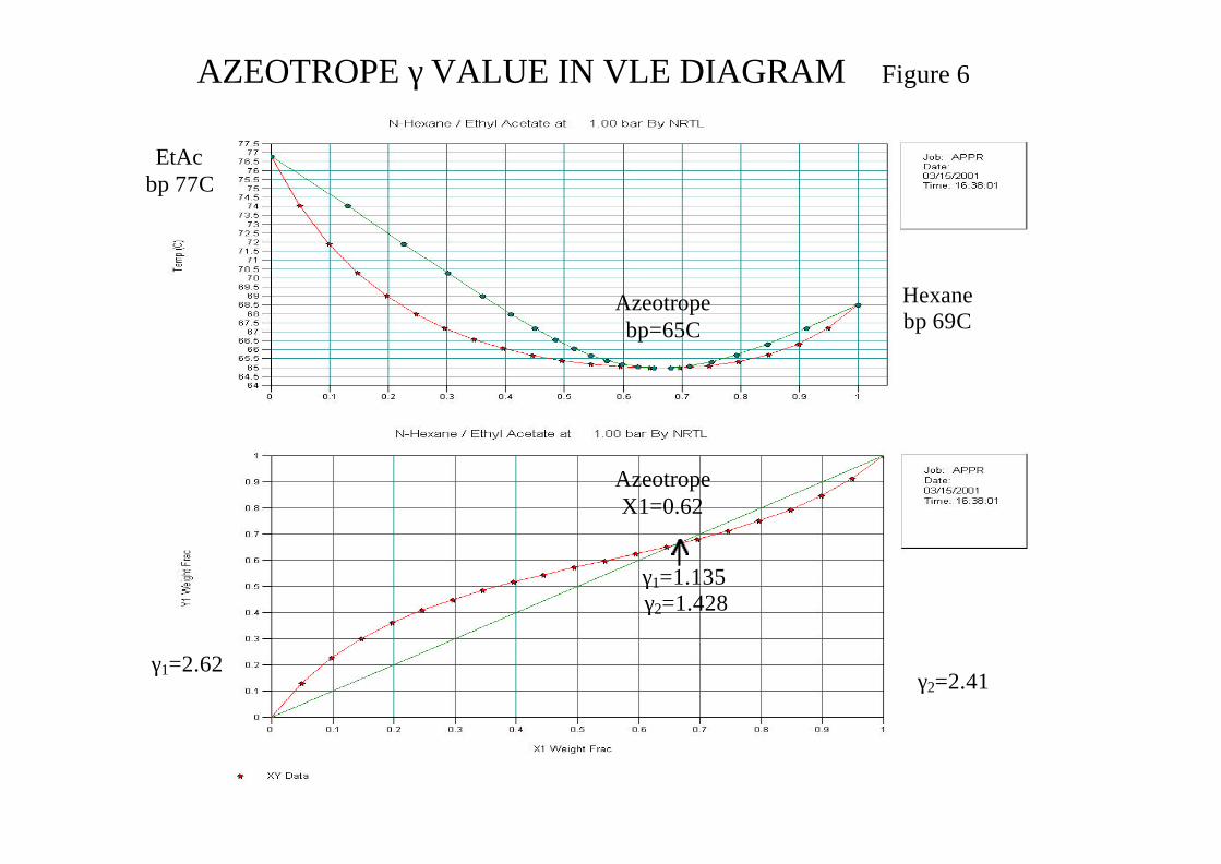
AZEOTROPE γ VALUE IN VLE DIAGRAM Figure 6
Hexane bp 69C
EtAc bp 77C
Azeotrope X1=0.62
Azeotrope bp=65C
γ1=2.62 γ2=2.41
γ2=1.428 γ1=1.135
VLE DIAGRAM AND CONVERGENCE EFFECTS Figure 7
CHEMCAD K AND H VALUES WIZARD Figure 8
?
?
P
K=PSRK H=MIXH
?
K=VAP H=SRK
K=VAP H=LATE
SINGLE
CHEMICAL OTHER
MULTI
CHEM<200 PSI OTHER
CH
EM
>20
0 P
SI
<7BAR
HE
AV
Y H
C
>7BAR
AMINE K=AMINE H=AMINE
SOUR K=SOUR H=SRK
POLYMER K=UPLM H=LATE
HCL/NH3 K=PPAQ H=SRK
HTSL
K=ESSO 90 to 200C
H=LK
K=GS (P<200BAR)
H=LK
Data>50% NRTL,Wilson
UNIQUAC Data<50% UNIFAC
H=LATE (all)
K=PR H=PR
<-70C
K=SRK H=SRK
>-70C
SPECIAL METHODS
T
COMP
THERMODYNAMIC MODEL DECISION TREE Figure 9
?
?
?
IDEAL VAP PRESS GAS EQUATION
BIP MODEL
BIP MODEL LLE BIPS
NRTL (5 PAR) UNIQUAC (2 PAR) UNIFAC(INCREM)
?
PENG ROBINSON
BENEDICT WEBB RUBIN
GAS EQUATIONSOAVE
REDLICH KWONG(SRK)
GAS
VAP ONLY NAT GAS
LIQUID
LIQUID LLE
HY
DR
OC
AR
BO
N
AZ
EO
TR
OP
E
NOV
LE
YES
NRTL (5 PAR) UNIQUAC (2 PAR) UNIFAC(INCREM)
H=LATENT HEAT
H=LATENT HEAT H=LATENT HEAT
H=LATENT HEATH=LEE KESSLER
H=LEE KESSLER
H=LATENT HEAT
IDEAL VAPOR
PHASE
IDEAL
SET THERMODYNAMIC MODEL Figure 10