Embed Size (px)
Citation preview

Process of Seismic Simulation of a 2-bay, 2-story Reinforced Concrete Building
Michelle Stadel1, Yashar Moslehy2, A. Laskar3, and Y.L. Mo4
Abstract
Computer simulation through such programs as OpenSees is an effective method
for studying earthquake engineering. Three key aspects of OpenSees code are modeling,
recorders and analysis. A two-story, two-bay reinforced concrete building will be tested
with multi-directional loads and the displacement simulated with computers. The
structure can be modeled in OpenSees and programmed to output the loads and the
corresponding displacements.
1.0 Introduction
Earthquakes impact reinforced concrete structures in various ways. Structural
engineers need to be able to model these effects in order to design better RC structures
that can withstand earthquakes and preserve lives. Computer simulations are the most
cost-effective way to predict and study buildings subjected to earthquake loading.
One such program is OpenSees, which is a finite element framework developed
by the University of California Berkeley in conjunction with the Pacific Earthquake
Engineering Research Center (PEER 2001). Previous research has shown that OpenSees
can effectively model structures and the impact of earthquake loading (Howser 2007).
1 Department of Civil Engineering, South Dakota School of Mines & Technology, Rapid City, SD 57701 Email: [email protected] 2 Department of Civil and Environmental Engineering, University of Houston, TX, 77204-4003 Email: [email protected] 3 Department of Civil and Environmental Engineering, University of Houston, Houston, 77204-4003 Email: [email protected] 4 Department of Civil and Environmental Engineering, University of Houston, Houston, 77204-4003 Email: [email protected], Ph # 713-743-4274, Fax # 713-743-4260

2
The National Center for Research on Earthquake Engineering (NCREE) in
Taiwan has prepared a near full-scale, two-story, two-bay RC building to test with multi-
directional loading. Researchers at the University of Houston are preparing a program in
OpenSees to model this structure in order to correlate future analytical tools and new
design methods (Hwang, et. al 2006). This paper will look at the process to develop such
a program in OpenSees and the analysis of the results generated.
2.0 Simulation of Concrete Structure
OpenSees stands for Open System for Earthquake Engineering Simulation. The
program is an open framework that allows users to develop code for modeling buildings
and soils in earthquake scenarios. OpenSees uses Tcl/Tk script to develop programs. Tcl
or Tool Command Language is a string-based scripting language that means an
expression can always be seen as a numeric value, a string or another value. Tk is the
graphical extension (Schwerd 2006).
Developing code first requires understanding the main objects needed to create an
OpenSees program. The three objects are modeling, analysis and output generation
(Mazzoni 2006). To better understand these concepts, a two-dimensional structure was
modeled and analyzed.
A two-bay, two-dimensional frame, as shown in Figure 1, was used in order to
correlate the concepts necessary for developing an OpenSees program with the NCREE
model. OpenSees does not have a two-bay frame; therefore, it was necessary to create
one.

3
2.1 Modeling the structure
The first step in modeling any structure is to choose a coordinate system. Nodes,
points located on the structure can be easily labeled with a coordinate system originating
from node 1. Modeling requires establishing the position of nodes in order to link the
model together. The simplest node arrangement is to place one at each beam and column
intersection. For this problem, each beam was made up of four nodes and each column
had three nodes, one at each end and one in the center.
Each beam and column will be made up of different materials arranged in a
different fashion; therefore, it is necessary to define the cross-sections for both the beams
and the columns. To create a cross-section in OpenSees, the section command, which
represents force-deformation relationships at beam-column points, is used. Furthermore,
the cross-sections were defined as fibers, a command which creates smaller regions for
which the material’s stress-strain response is integrated to give resultant behavior
(Mazzoni 2006). The fiber command is perfect for reinforced concrete to establish the
locations of materials such as cover concrete, core concrete and rebar in the cross-section.
The element command is the key to linking the nodes and the cross-sections
together. OpenSees contains ten different types of elements. In this scenario, nonlinear
beam-column elements were used to represent both beams and columns. These objects
were classified as nonlinear beam-columns because of the force formulation and the
spread of plasticity along the element. An element requires a unique element tag, two
different nodes to be linked, the number of integration points, the section tag or the
number that corresponds to the correct cross-section and the value that corresponds to the
correct coordinate transformation (Mazzoni 2006).

4
The user must be sure to check units because OpenSees does not keep track of
units. Units were a problem in this example because the dimensions were metric and the
material properties were in English units. It was decided to convert all frame dimensions
from millimeters to inches.
2.1.1 Dimensions and cross-sections
Each column is 3,000 mm high with a 300 mm deep by 400 mm wide cross-
section, as shown in Figure 2a. The stirrups in the columns were No. 3 rebar spaced at
200 mm on center in addition to three rows of No. 7 rebar running the entire vertical
length of the column. All reinforcement was covered with at least 50 mm of concrete
Each beam was 4,000 mm in length and consisted of the same cross-sectional
area. The beams were 200 mm deep and 350 mm high. Reinforcement was again No. 3
rebar spaced at 250 mm on center. Two, No. 7 rebars run across the top of the beam
while the bottom row contained four bars as shown in Figure 2b.
2.1.2 Material properties
Defining the concrete properties was the next step in the model. The core concrete
of each section differed from the outside, cover concrete. The core concrete had a
measured 28-day compressive strength of 6.0 psi and a strain of 0.004 at max strength. At
the point of crushing, the concrete had a measured strength of 5.0 psi and a strain of
0.014.
The 50 millimeters of cover concrete had a 5.0 psi 28-day compressive strength.
A strain of 0.002 was measured at max strength. No crushing strength was found, but a
strain of 0.006 was measured.

5
The reinforcing steel had a yield stress of 60.0 psi and a modulus of elasticity, E,
of 30,000 psi. No. 7 rebar has an area of 0.6 in2. The steel also had a strain hardening
ratio of 0.01.
Material properties were classified by the uniaxialMaterial command. The
concrete was represented by Concrete01, a zero tensile strength concrete. The reinforcing
steel was represented by Steel01, which is a uniaxial bilinear steel material object
(Mazzoni 2006). Also properties based on compression are entered as negative numbers.
2.1.3 Loading
Since earthquake loading acts in the horizontal direction, a lateral load of 100 kips
was applied to the top right corner (node 15) of Figure 1. In simulating a real-life model,
gravity loads should also be applied to the structure at this time, but for simplification of
the scenario, gravity loads were ignored.
2.2 Recorder generation
The purpose of this example is to find when the structure fails with this loading.
So the next step is to generate recorders that will output the displacement. The node
recorder and the element recorder are perhaps the most essential commands for
generating data in a pushover analysis. The recorder command generates a file which can
be opened in a database program and analyzed. Using the recorder plot command, it is
also possible to watch the data that is being stored in the file be graphed as it is obtained.
This can be useful in determining if the program is generating reasonable responses.

6
2.3 Analysis
The analysis object is the last piece of the code generated. Analysis consists of six
components: constraint handler, degrees of freedom numberer, analysis model, integrator,
the solution algorithm and the system of equations.
First, the system of equations can be defined. This specifies how to store and
solve the system of equations for the analysis. Banded general was used to create an un-
symmetric banded system of equations object which will be factored and solved during
the analysis using the Lapack band general solver (Mazzoni 2006).
Second, the constraint handler, which tells OpenSees how to handle the boundary
conditions and imposed displacements, can be defined. The transformation method was
employed which reduces the size of the system for multi-point constraints.
Third, a numberer, either plain or a Reverse Cuthill-McKee (RCM) algorithm, is
chosen. For this example, the RCM numberer was used because this is the best algorithm
for large problems and will output a warning when the structure is disconnected.
Fourth, a normal displacement increment test was chosen for the convergence
test. This command requires a convergence tolerance and the maximum number of
iterations to be performed before failure to converge is returned, to be defined. Fifty
iterations and a convergence tolerance of 1.0e-12 were used in this analysis.
Fifth, the user must specify the solution algorithm that will be used to solve the
non-linear equation. For this example, the Newton-Raphson method was used to advance
to the next time step.
Finally, the integrator is chosen. In this case, displacement control was used to
help narrow down the results. This command uses a specified displacement increment to

7
find the load at that displacement for the specified load. In this case, an increment of 0.1
was applied to node 15.
Before running the program, the user must define the type of analysis and the
number of iterations for the analysis to run. In this case, a static analysis was chosen and
fifty iterations were used. The complete program code for this example can be found in
appendix A.
3.0 Simulation of the Subject Building
3.1 Modeling the structure
Many basic elements of modeling remained the same for this structure. Major
differences include nodes only at beam-column intersections, shear walls, section
aggregators, loading, and the type of material properties in the shear walls.
Shear walls are introduced in this model. These are modeled using the standard
brick element as will be discussed later. For the shear walls, a different type of material
was introduced, nDMaterial. This command constructs an object which represents stress-
strain relationships at integration points of force-deformation elements (Mazzoni 2006).
The Elastic Isotropic Material was used because it can model a plane stress element
which is what the shear walls are. The shear walls are modeled as plane stress elements
because one of the principal stresses is zero.
Beams and columns were again modeled as nonlinear beam-columns. In addition,
to compensate for torsion that might occur with the presence of the shear walls, section
aggregators were incorporated.

8
3.1.1 Dimensions and cross-sections
In order to describe this structure, it is important to define some terms and
positioning. Column line A refers to the columns supporting the shear wall or the left side
of Figure 3. Column line B is the center columns and column line C is the remaining two
columns on the right side of Figure 3. Column lines A and B are 5,500 mm apart and the
distance from columns B to C is 3,500 mm. So the length of the entire structure or the
distance from A to C is 9,000 mm.
The columns are 4,300 mm high. The distance from the ground to the first floor
slab is 2,200 mm and the distance between floors is 1,900 mm. The columns have a 400
mm square cross-section, as shown in Figure 4a. There are four rows of No. 6 rebar, four
bars in each of the top and bottom rows and two bars in each of the remaining middle
rows. Stirrups are No. 3 rebar, spaced 300 mm apart.
Beam cross sections are 400 mm high and 300 mm across. The beams are
reinforced by four rows of rebar each containing two bars of No. 6 rebar as shown in
Figure 4b. Stirrups made of No. 3 rebar are spaced 100 mm apart.
3.1.2 Material properties
Defining the material properties for the beams and columns was the next step. The
core concrete and the concrete covering the rebar had slightly different properties. The
core concrete had a measured 28-day compressive strength of 34.8 Pascals and a strain of
0.003 at max strength. At the point of crushing, the concrete had a measured strength of
27.5 Pa and a strain of 0.002. The concrete was again modeled by the uniaxial material
concrete01.

9
The 50 millimeters of cover concrete had a 27.5 Pa 28-day compressive strength.
A strain of 0.003 was measured at max strength. A crushing strength of 2.75 Pa was
found along with a strain of 0.006 at crushing. The concrete was also modeled by the
uniaxial material concrete01.
The reinforcing steel had a yield stress of 659 Pa and a modulus of elasticity, E, of
200,000 Pa. No. 7 rebar has an area of 387.1 mm2 (0.6 in2). The steel also had a strain
hardening ratio of 0.017. The steel was again modeled by the uniaxial material steel01.
3.1.3 Shear Walls
The shear walls were reinforced concrete plane stress elements and were modeled
with the standard brick element. The standard brick element creates an eight-node brick
object. Each shear wall was represented by two bricks each one-half the thickness of the
shear wall.
3.1.4 Loading
Four lateral loads were applied to this frame. Nodes 3 and 4, which are the nodes
at the first floor slab on the right side of Figure 3, loaded with 6,000 N. Nodes 5 and 6,
the nodes on the second floor slab directly above the previous two, were loaded with
twice the amount, 12,000 N.
3.2 Recorder generation
Node recorders were created to monitor the displacements at the nodes where the
loads were being applied. Results for this model were based on the displacement of one
of the top nodes, node 6.

10
3.3 Analysis
The same analysis procedure, previously described for the 2D frame, was used
except for the factors associated with the convergence test and the displacement intervals.
The convergence tolerance was set at 1.0e-2. In addition, the test was supposed to
conduct 5,000 iterations before returning a “failure to converge” message. The
displacement was controlled by node 6 at intervals of 0.001 mm. The complete code used
for this frame can be found in Appendix B.
4.0 Simulated Results
Each program was set to output the displacement increment and the
corresponding load step. Graphing the displacement versus the load produces a stress-
strain curve also called a backbone curve.
4.1 Simple 2D structure
Analysis of the output file generates a stress-strain curve, otherwise known as a
backbone curve. The stress-strain curve for the 2D structure, as shown in Figure 5, has an
ultimate strength of approximately 64 kips. The output file shows that rupture occurred
around 63.4 kips. A modulus of elasticity of 40 ksi can be calculated based on the
straight-line portion of the curve.
4.2 NCREE model
The stress-strain curve generated from the code for the NCREE structure can be
found in Figure 6. Results show an ultimate strength of 650 kN. The material ruptures at
284 kN. From calculating the slope of the straight-line portion of the graph, a modulus of
elasticity of 498 GPa can be found.

11
5.0 Conclusions
OpenSees is a valuable tool for studying the effects of earthquakes on reinforced
concrete structures. Programs can be generated to output the displacement and the
loading. From the output files, stress-strain curves can be developed.
Time constraints limited the scope of this research to studying the process
necessary to develop a simulation of the structure. Further development of this code
might include adding gravity loads and cyclic loading to completely study the results of
earthquake loading on the shear walls. Currently, the code to study the cyclic loading is
being developed by Dr. Y.L. Mo’s researchers.
6.0 Acknowledgements
The research study described herein was sponsored by the National Science
Foundation under the Award No. EEC-0649163. The opinions expressed in this study are
those of the authors and do not necessarily reflect the views of the sponsor.
7.0 References
Howser, Rachel, A. Laskar, Y.L. Mo. (2007) “Seismic Interaction of Flexural Ductility and Shear Capacity in Reinforced Concrete Columns.”
Hwang, S.J., M. Saiid Saiidi, Sara Wadia-Fascetti, JoAnn Browning, Jerry P. Lynch, Kamal Tawfig, K.C. Tsai, G. Song, Y.L. Mo. (2006) “Experiments and Simulation of Reinforced Concrete Buildings Subjected to Reversed Cyclic Loading and Shake Table Excitation.”
Mazzoni, Silvia, Frank McKenna, Michael H. Scott, Gregory L. Fenves, et. al. (2006). “Open System for Earthquake Engineering Simulation User Command-Language Manual,” Pacific Earthquake Engineering Research Center, UC Berkeley, http://opensees.berkeley.edu/OpenSees/manuals/usermanual/index.html.
Pacific Earthquake Engineering Research Center (PEER). (2001) “Open System for Earthquake Engineering Simulation.” http://peer.berkeley.edu/news/2001spring/opensees.html
Schwerd, Daniel. (2006) “Scriptics.com – the Script Archive.” http://dev.scriptics.com/software/tcltk/.
Tseng, Chien-Chuang. (2006) Experiment of Reinforced Concrete Building Frame Presentation.

12
8.0 List of Tables and Figures Figure 1 – 2D Frame ……………………………………………………………… 12 Figure 2 – 2D Frame cross-sections …………………………………………….… 12 Figure 3 – NCREE frame …………………………………………………………. 13 Figure 4 – NCREE frame cross-sections ………………………………….……… 13 Figure 5 – 2D Frame stress-strain curve …………………………………….……. 14 Figure 6 – NCREE frame stress-strain curve ………………………………..……. 14
Figure 1 A drawing of the 2D frame problem.
(a) (b)
Figure 2 Cross-sectional views of (a) the columns and (b) the beams of the 2D frame. The column cross-section represents the line AA on Figure 1 while the beam cross-section comes from line BB.

13
Figure 3 A drawing of the two-bay, two-story reinforced concrete building constructed at the National Center for Research on Earthquake Engineering (Tseng).
(a) (b)
Figure 4 Cross-sectional views of (a) the columns and (b) the beams of the two-bay, two-story reinforced concrete structure (Tseng).

14
0
10
20
30
40
50
60
70
0 2 4 6 8 10 12
Displacement (inches)
Load
(kip
s)
Figure 5 Stress-Strain Curve for 2D Frame
0
100
200
300
400
500
600
700
0 1 2 3 4 5Displacement (mm)
Load
(kN)
Figure 6 Stress-Strain Curve for NCREE structure based on displacement at Node 6.

15
Appendix A
# 2D frame example problem # Units: kips, inches model basic -ndm 2 -ndf 3 # Define nodes ------------------------- set width 315.0 set height 118.1 # Define some parameters set x1 [expr $width/2] set y1 [expr $height/2] # node tag X Y node 1 0 0 node 2 $x1 0 node 3 $width 0 node 4 0 $y1 node 5 $x1 $y1 node 6 $width $y1 node 7 0 $height node 8 [expr $width/8] $height node 9 [expr $x1/2] $height node 10 [expr 3*$x1/4] $height node 11 $x1 $height node 12 [expr 5*$width/8] $height node 13 [expr 3*$width/2] $height node 14 [expr 7*$width/8] $height node 15 $width $height # Fix constraints fix 1 1 1 1 fix 2 1 1 1 fix 3 1 1 1 # Define MATERIALS # ------------------------- # CONCRETE tag f'c epsc0 f’cu epsU # Core Concrete (confined) uniaxialMaterial Concrete01 1 -6.0 -0.004 -5.0 -0.014 # Cover concrete (unconfined) uniaxialMaterial Concrete01 2 -5.0 -0.002 0.0 -0.006 # STEEL # Reinforcing Steel set fy 60.0; # Yield stress set E 30000.0; # Young's modulus # tag fy E0 b

16
uniaxialMaterial Steel01 3 $fy $E 0.01 # Define Column cross-section # ------------------------------------ # Column parameters set cWidth 15.7; # column width set cDepth 11.8; # column height set cover 2.0; # cover set As7 0.6; # area of no. 7 bars # Variables derived from parameters set cy1 [expr $cDepth/2.0] set cz1 [expr $cWidth/2.0] # Create a Uniaxial Fiber object section Fiber 1 { # Create the concrete core fibers # patch rect $matTag $numSubdivIJ $numSubdivJK $yI $zI $yJ $zJ $yK $zK $yL $zL patch rect 1 10 1 [expr $cover-$cy1] [expr $cover-$cz1] [expr $cy1-$cover] [expr $cz1-$cover]; # Create the concrete cover fibers (top, bottom, left, right) patch rect 2 10 1 [expr -$cy1] [expr $cz1-$cover] $cy1 $cz1; patch rect 2 10 1 [expr -$cy1] [expr -$cz1] $cy1 [expr $cover-$cz1]; patch rect 2 2 1 [expr -$cy1] [expr $cover-$cz1] [expr $cover-$cy1] [expr $cz1-$cover]; patch rect 2 2 1 [expr $cy1-$cover] [expr $cover-$cz1] $cy1 [expr $cz1-$cover]; # Create the reinforcing fibers (3 layers) # layer straight $matTag $numBars $areaBar $yStart $zStart $yEnd $zEnd layer straight 3 3 $As7 [expr $cy1-$cover] [expr $cover-$cz1] [expr $cover-$cy1] [expr $cover-$cz1] layer straight 3 2 $As7 $cy1 0 [expr -$cy1] 0 layer straight 3 3 $As7 $cy1 [expr $cy1-$cover] [expr -$cy1] [expr $cz1-$cover] } # Define beam cross-section # ------------------------------------ # Beam parameters set bWidth 7.9; # beam width set bDepth 13.8; # beam height # Variables derived from parameters set by1 [expr $bDepth/2.0] set bz1 [expr $bWidth/2.0] # Create a Uniaxial Fiber object

17
section Fiber 2 { # Create the concrete core fibers # patch rect $matTag $numSubdivIJ $numSubdivJK $yI $zI $yJ $zJ $yK $zK $yL $zL patch rect 1 10 1 [expr $cover-$by1] [expr $cover-$bz1] [expr $by1-$cover] [expr $bz1-$cover]; # Create the concrete cover fibers (top, bottom, left, right) patch rect 2 10 1 [expr -$by1] [expr $bz1-$cover] $by1 $bz1; patch rect 2 10 1 [expr -$by1] [expr -$bz1] $by1 [expr $cover-$bz1]; patch rect 2 2 1 [expr -$by1] [expr $cover-$bz1] [expr $cover-$by1] [expr $bz1-$cover]; patch rect 2 2 1 [expr $by1-$cover] [expr $cover-$bz1] $by1 [expr $bz1-$cover]; # Create the reinforcing fibers (top, bottom) # layer straight $matTag $numBars $areaBar $yStart $zStart $yEnd $zEnd layer straight 3 2 $As7 [expr $by1-$cover] [expr -$bz1] [expr $cover-$by1] [expr -$bz1] layer straight 3 4 $As7 [expr $by1-$cover] $bz1 [expr $cover-$by1] $bz1 } # Define Columns ----------------------------------- geomTransf Linear 1 # element nonlinearBeamColumn $eleTag $iNode $jNode $numIntgrPts $secTag $transfTag element nonlinearBeamColumn 1 1 4 2 1 1 element nonlinearBeamColumn 2 4 7 2 1 1 element nonlinearBeamColumn 3 2 5 2 1 1 element nonlinearBeamColumn 4 5 11 2 1 1 element nonlinearBeamColumn 5 3 6 2 1 1 element nonlinearBeamColumn 6 6 15 2 1 1 # Define Beams ------------------------------------ geomTransf Linear 2 # element nonlinearBeamColumn $eleTag $iNode $jNode $numIntgrPts $secTag $transfTag element nonlinearBeamColumn 7 7 8 3 2 2 element nonlinearBeamColumn 8 8 9 3 2 2 element nonlinearBeamColumn 9 9 10 3 2 2 element nonlinearBeamColumn 10 10 11 3 2 2 element nonlinearBeamColumn 11 11 12 3 2 2 element nonlinearBeamColumn 12 12 13 3 2 2 element nonlinearBeamColumn 13 13 14 3 2 2
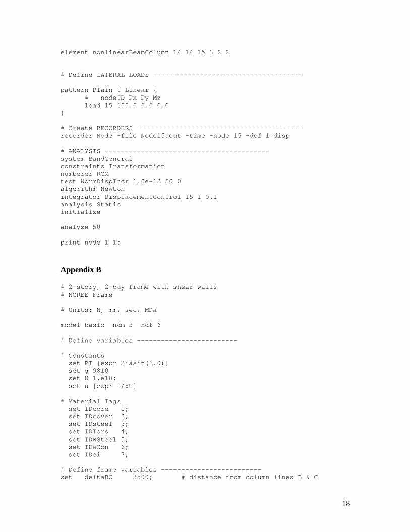
18
element nonlinearBeamColumn 14 14 15 3 2 2 # Define LATERAL LOADS ------------------------------------- pattern Plain 1 Linear { # nodeID Fx Fy Mz load 15 100.0 0.0 0.0 } # Create RECORDERS ----------------------------------------- recorder Node -file Node15.out -time -node 15 -dof 1 disp # ANALYSIS ----------------------------------------- system BandGeneral constraints Transformation numberer RCM test NormDispIncr 1.0e-12 50 0 algorithm Newton integrator DisplacementControl 15 1 0.1 analysis Static initialize analyze 50 print node 1 15
Appendix B
# 2-story, 2-bay frame with shear walls # NCREE Frame # Units: N, mm, sec, MPa model basic -ndm 3 -ndf 6 # Define variables ------------------------- # Constants set PI [expr 2*asin(1.0)] set g 9810 set U 1.e10; set u [expr 1/$U] # Material Tags set IDcore 1; set IDcover 2; set IDsteel 3; set IDTors 4; set IDwSteel 5; set IDwCon 6; set IDei 7; # Define frame variables ------------------------- set deltaBC 3500; # distance from column lines B & C

19
set deltaAB 5500; # distance between column lines A & B set deltaAC 9000; # distance between column lines A & C set delta12 3000; # distance from node 1 to node 2 set CH1 2200; # height to center of 2nd floor slab set CH2 4100; # height to center of 3rd floor slab # Create nodes ------------------------- node 1 0 0 0 node 2 0 $delta12 0 node 3 0 0 $CH1 node 4 0 $delta12 $CH1 node 5 0 0 $CH2 node 6 0 $delta12 $CH2 node 7 $deltaBC 0 0 node 8 $deltaBC $delta12 0 node 9 $deltaBC 0 $CH1 node 10 $deltaBC $delta12 $CH1 node 11 $deltaBC 0 $CH2 node 12 $deltaBC $delta12 $CH2 node 13 $deltaAC 0 0 node 14 $deltaAC $delta12 0 node 15 $deltaAC 0 $CH1 node 16 $deltaAC $delta12 $CH1 node 17 $deltaAC 0 $CH2 node 18 $deltaAC $delta12 $CH2 # Fix supports fix 1 1 1 1 1 1 1; # fully fixed fix 2 1 1 1 1 1 1; fix 13 1 1 1 1 1 1; fix 14 1 1 1 1 1 1; fix 7 1 1 1 1 1 1; fix 8 1 1 1 1 1 1; # Define materials ------------------------- # Define property variables set fc [expr -27.5]; set Ec [expr 4700.*sqrt(-$fc)]; set fc1C [expr 1.26394*$fc]; set eps1C [expr 2.*$fc1C/$Ec]; set fc2C $fc; set eps2C [expr 2.*$fc2C/$Ec]; set fc1U $fc; set eps1U -0.003; set fc2U [expr 0.1*$fc]; set eps2U -0.006; set v 0.15; # Poisson's Ratio set Fy 411.9; # yield stress set Es 200000; # modulus of elasticity set epsY [expr $Fy/$Es] set Fy1 559.; set epsY1 0.03;

20
set Fu 659.0; set epsU 0.08; set rou 0.017; # Core Concrete uniaxialMaterial Concrete01 $IDcore $fc1C $eps1C $fc2C $eps2C; # Cover Concrete uniaxialMaterial Concrete01 $IDcover $fc1U $eps1U $fc2U $eps2U; # Reinforcing Steel uniaxialMaterial Steel01 $IDsteel $Fy $Es $rou # Column element # ----------------------------------------------- # Column parameters set cWidth 400.0; # column width set cDepth 400.0; # column height set cover 50.0; # cover set As6 285.0; # area of no. 6 bars # Variables derived from the parameters set cy1 [expr $cDepth/2.0]; set cz1 [expr $cWidth/2.0]; # Create a Uniaxial Fiber object section Fiber 2 { # Create the concrete core fibers # mat num num patch rect $IDcore 2 2 [expr $cover-$cy1] [expr $cover-$cz1] [expr $cy1-$cover] [expr $cz1-$cover]; # Create the concrete cover fibers (top, bottom, left, right) patch rect $IDcover 2 2 [expr -$cy1] [expr $cz1-$cover] $cy1 $cz1; patch rect $IDcover 2 2 [expr -$cy1] [expr -$cz1] $cy1 [expr $cover-$cz1]; patch rect $IDcover 2 2 [expr -$cy1] [expr $cover-$cz1] [expr $cover-$cy1] [expr $cz1-$cover]; patch rect $IDcover 2 2 [expr $cy1-$cover] [expr $cover-$cz1] $cy1 [expr $cz1-$cover]; # Create the reinforcing fibers (4 layers) layer straight $IDsteel 4 $As6 [expr $cy1-$cover] [expr $cz1-$cover] [expr $cy1-$cover] [expr $cover-$cz1]; layer straight $IDsteel 2 $As6 [expr -($cWidth-2*$cover)/6] [expr $cz1-$cover] [expr -($cWidth-2*$cover)/6] [expr $cover-$cz1]; layer straight $IDsteel 2 $As6 [expr ($cWidth-2*$cover)/6] [expr $cz1-$cover] [expr ($cWidth-2*$cover)/6] [expr $cover-$cz1]; layer straight $IDsteel 4 $As6 [expr $cover-$cy1] [expr $cz1-$cover] [expr $cover-$cy1] [expr $cover-$cz1]; }

21
# Beam element # ----------------------------------------------- # Beam paramaters set bWidth 300.0; # beam width set bDepth 400.0; # beam height # Variables derived from the parameters set by1 [expr $bDepth/2.0]; set bz1 [expr $bWidth/2.0]; # Create a Uniaxial Fiber object section Fiber 4 { # Create the concrete core fibers # mat num num patch rect $IDcore 2 2 [expr $cover-$by1] [expr $cover-$bz1] [expr $by1-$cover] [expr $bz1-$cover]; # Create the concrete cover fibers (top, bottom, left, right) patch rect $IDcover 2 2 [expr -$by1] [expr $bz1-$cover] $by1 $bz1; patch rect $IDcover 2 2 [expr -$by1] [expr -$bz1] $by1 [expr $cover-$bz1]; patch rect $IDcover 2 2 [expr -$by1] [expr $cover-$bz1] [expr $cover-$by1] [expr $bz1-$cover]; patch rect $IDcover 2 2 [expr $by1-$cover] [expr $cover-$bz1] $by1 [expr $bz1-$cover]; # Create the reinforcing fibers (4 layers) layer straight $IDsteel 2 $As6 [expr $by1-$cover] [expr $bz1-$cover] [expr $by1-$cover] [expr $cover-$bz1]; layer straight $IDsteel 2 $As6 [expr -($bWidth-2*$cover)/6] [expr $bz1-$cover] [expr -($bWidth-2*$cover)/6] [expr $cover-$bz1]; layer straight $IDsteel 2 $As6 [expr ($bWidth-2*$cover)/6] [expr $bz1-$cover] [expr ($bWidth-2*$cover)/6] [expr $cover-$bz1]; layer straight $IDsteel 2 $As6 [expr $cover-$by1] [expr $bz1-$cover] [expr $cover-$by1] [expr $cover-$bz1]; } # Create section aggregators (puts torsion in sections) # ----------------------------------------------------- set G $U; # shear modulus -- describes an object's tendency to shear set J 1.; set GJ [expr $G*$J] uniaxialMaterial Elastic $IDTors $GJ set IDcolSec 1 set IDbeamSec 3 # tag uniTag uniCode secTag section Aggregator $IDcolSec $IDTors T -section 2 section Aggregator $IDbeamSec $IDTors T -section 4

22
# Create columns # ------------------------- geomTransf Linear 1 0 1 0 # element nonlinearBeamColumn $eleTag $iNode $jNode $numIntgrPts $secTag $transfTag element nonlinearBeamColumn 1 1 3 3 $IDcolSec 1 element nonlinearBeamColumn 2 3 5 3 $IDcolSec 1 element nonlinearBeamColumn 3 2 4 3 $IDcolSec 1 element nonlinearBeamColumn 4 4 6 3 $IDcolSec 1 element nonlinearBeamColumn 5 7 9 3 $IDcolSec 1 element nonlinearBeamColumn 6 9 11 3 $IDcolSec 1 element nonlinearBeamColumn 7 8 10 3 $IDcolSec 1 element nonlinearBeamColumn 8 10 12 3 $IDcolSec 1 element nonlinearBeamColumn 9 13 15 3 $IDcolSec 1 element nonlinearBeamColumn 10 15 17 3 $IDcolSec 1 element nonlinearBeamColumn 11 14 16 3 $IDcolSec 1 element nonlinearBeamColumn 12 16 18 3 $IDcolSec 1 # Create beams # ------------------------- geomTransf Linear 2 0 0 -1 element nonlinearBeamColumn 13 3 4 3 $IDbeamSec 2 element nonlinearBeamColumn 14 5 6 3 $IDbeamSec 2 element nonlinearBeamColumn 15 9 10 3 $IDbeamSec 2 element nonlinearBeamColumn 16 11 12 3 $IDbeamSec 2 element nonlinearBeamColumn 17 17 18 3 $IDbeamSec 2 element nonlinearBeamColumn 18 3 9 3 $IDbeamSec 2 element nonlinearBeamColumn 19 9 15 3 $IDbeamSec 2 element nonlinearBeamColumn 20 5 11 3 $IDbeamSec 2 element nonlinearBeamColumn 21 11 17 3 $IDbeamSec 2 element nonlinearBeamColumn 22 4 10 3 $IDbeamSec 2 element nonlinearBeamColumn 23 10 16 3 $IDbeamSec 2 element nonlinearBeamColumn 24 6 12 3 $IDbeamSec 2 element nonlinearBeamColumn 25 12 18 3 $IDbeamSec 2 # --------------------------------------------------------------------- # Create ModelBuilder for 3D elements in Y-Z Plane # --------------------------------------------------------------------- model basic -ndm 3 -ndf 3 # Create nodes node 20 9075 0 0 node 21 9000 0 0 node 22 8925 0 0 node 23 9075 3000 0
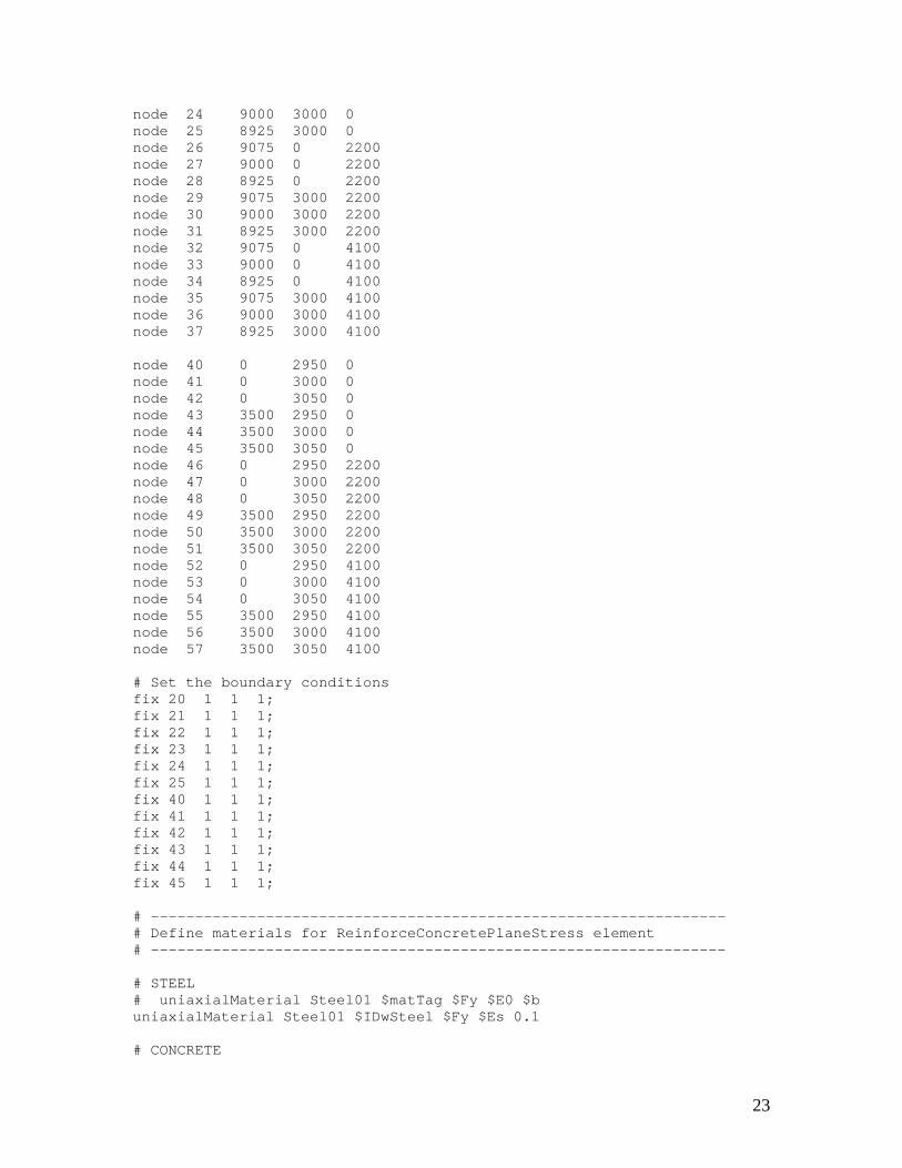
23
node 24 9000 3000 0 node 25 8925 3000 0 node 26 9075 0 2200 node 27 9000 0 2200 node 28 8925 0 2200 node 29 9075 3000 2200 node 30 9000 3000 2200 node 31 8925 3000 2200 node 32 9075 0 4100 node 33 9000 0 4100 node 34 8925 0 4100 node 35 9075 3000 4100 node 36 9000 3000 4100 node 37 8925 3000 4100 node 40 0 2950 0 node 41 0 3000 0 node 42 0 3050 0 node 43 3500 2950 0 node 44 3500 3000 0 node 45 3500 3050 0 node 46 0 2950 2200 node 47 0 3000 2200 node 48 0 3050 2200 node 49 3500 2950 2200 node 50 3500 3000 2200 node 51 3500 3050 2200 node 52 0 2950 4100 node 53 0 3000 4100 node 54 0 3050 4100 node 55 3500 2950 4100 node 56 3500 3000 4100 node 57 3500 3050 4100 # Set the boundary conditions fix 20 1 1 1; fix 21 1 1 1; fix 22 1 1 1; fix 23 1 1 1; fix 24 1 1 1; fix 25 1 1 1; fix 40 1 1 1; fix 41 1 1 1; fix 42 1 1 1; fix 43 1 1 1; fix 44 1 1 1; fix 45 1 1 1; # ----------------------------------------------------------------- # Define materials for ReinforceConcretePlaneStress element # ----------------------------------------------------------------- # STEEL # uniaxialMaterial Steel01 $matTag $Fy $E0 $b uniaxialMaterial Steel01 $IDwSteel $Fy $Es 0.1 # CONCRETE

24
# uniaxialMaterial Concrete01 $matTag $fpc $epsc0 $fpcu $epsU uniaxialMaterial Concrete01 $IDwCon $fc1C $eps1C $fc2C $eps2C set rouw 0.0015 set pi 3.141592654; # NDMaterial: ReinforceConcretePlaneStress # tag rho s1 s2 c1 c2 angle1 angle2 rou1 rou2 fpc fy E0 nDMaterial ElasticIsotropic $IDei $Ec $v # ----------------------------------------------------------------- # Define ReinforceConcretePlaneStress element # ----------------------------------------------------------------- # element stdBrick eletag node1 node2 node3 node4 node5 node6 node7 node8 mattag element stdBrick 30 22 25 24 21 28 31 30 27 $IDei element stdBrick 31 21 24 23 20 27 30 29 26 $IDei element stdBrick 32 28 31 30 27 34 37 36 33 $IDei element stdBrick 33 27 30 29 26 33 36 35 32 $IDei element stdBrick 40 41 44 43 40 47 50 49 46 $IDei element stdBrick 41 42 45 44 41 48 51 50 47 $IDei element stdBrick 42 47 50 49 46 53 56 55 52 $IDei element stdBrick 43 48 51 50 47 54 57 56 53 $IDei # tie nodes between beams, columns and walls equalDOF 13 21 1 2 3 equalDOF 14 24 1 2 3 equalDOF 15 27 1 2 3 equalDOF 16 30 1 2 3 equalDOF 17 33 1 2 3 equalDOF 18 36 1 2 3 equalDOF 2 41 1 2 3 equalDOF 8 44 1 2 3 equalDOF 4 47 1 2 3 equalDOF 10 50 1 2 3 equalDOF 6 53 1 2 3 equalDOF 12 56 1 2 3 # Redefine model ------------------------------------------- model basic -ndm 3 -ndf 6 # Define LATERAL LOADS ------------------------------------- pattern Plain 2 Linear { # nodeID Fx Fy Fz Mx My Mz load 3 6000 0 0 0 0 0 load 4 6000 0 0 0 0 0 load 5 12000 0 0 0 0 0 load 6 12000 0 0 0 0 0 } # Create RECORDERS ----------------------------------------- recorder Node -file basicframeNode3.out -time -node 3 -dof 1 disp recorder Node -file basicframeNode4.out -time -node 4 -dof 1 disp

25
# recorder Node -file basicframeNode5.out -time -node 5 -dof 1 disp recorder Node -file basicframeNode6.out -time -node 6 -dof 1 disp # recorder plot basicframeNode6.out Node_6_Xdisp 400 340 300 300 -columns 2 1 # ANALYSIS ----------------------------------------- system BandGeneral constraints Transformation numberer RCM test NormDispIncr 1.0e-2 5000 0 algorithm Newton integrator DisplacementControl 6 1 0.001 analysis Static initialize analyze 5000 print node 3 6