Embed Size (px)
Citation preview
Procyclical Government Spending inDeveloping Countries: The Role of Capital
Market Imperfections
Alvaro RiascosBanco de la Republica
Carlos A. VeghUCLA and NBER
Very preliminary draft: October 2003
Abstract
Whereas in the G-7 countries government consumption is essen-tially acyclical, in developing countries it appears to be highly pro-cyclical (i.e., government consumption rises in good times and falls inbad times). Several explanations have been advanced to explain thispuzzle, including political factors and borrowing constraints. Thispaper shows, however, that such differences in the procyclicality ofgovernment consumption are entirely consistent with a standard neo-classical model of fiscal policy in which policymakers optimally chooseboth the level of government consumption and taxes. We show that,with complete markets, the correlation of government consumptionand output is zero (as in G-7 countries). With only risk-free debt,however, this correlation is typically above 0.7, suggesting that thelack of a sufficiently rich menu of financial assets might be a majordeterminant of the way fiscal policy is carried out in developing coun-tries. Hence, the degree of market incompleteness is enough to explainthe above “puzzle” in a standard neoclassical fiscal model. Incom-plete markets are socially costly as they induce substantial volatilityin both private and public consumption, which would not be presentotherwise.
1
1 Introduction
A puzzling stylized fact related to the cyclical behavior of government con-sumption is that it appears to be much more procyclical in developing coun-tries than in industrial countries. In fact, Talvi and Végh (2000) report thatthe average correlation between the cyclical components of government con-sumption and output for 36 developing countries over the period 1970-1994 is0.53 compared to essentially zero for the G-7 countries. Remarkably, this cor-relation is positive in every developing country in their sample. Using morerefined econometric techniques, Braun (2001) finds ample support for thisphenomenon. Specifically, while in OECD countries a one percentage pointincrease in GDP is associated with a reduction of 0.37 percentage points inthe ratio of government expenditures to GDP, in developing countries thisratio remains unchanged. In other words, government expenditures increasesby the same proportion as output in expansions, while both fall by the sameproportion in recessions.The striking difference between government consumption being acyclical
for G-7 countries and highly procyclical for developing countries has beenviewed as inconsistent with the neoclassical paradigm of fiscal policy — à laBarro (1979) and Lucas and Stokey (1983) — and thus as a puzzle in search ofan explanation. Explanations have thus far followed under two main strands:(i) political pressures — which are exacerbated in developing countries bylarger political fragmentation and/or a more volatile tax base — may leadto higher spending in good times (Lane and Tornell (1999) and Talvi andVégh (2000)) and (ii) loss of access to international credit in difficult timesthat forces developing countries to contract government spending and raisetax rates in bad times (Gavin and Perotti (1997), Aizenman, Gavin, andHausmann (1996)).This paper starts from the idea that, whatever the merits of these exist-
ing explanations, one should not be too quick in dismissing the neoclassicalfiscal paradigm as being inconsistent with the stylized facts. In fact, we willargue in this paper that the cyclical behavior of government consumptionis entirely consistent with the neoclassical fiscal model. We will show thatall that is needed to explain the different behavior in developing and indus-trial countries is to recognize that the international credit markets faced byindustrial countries are more “complete” (in the Arrow-Debreu sense) thanthose facing developing countries. With complete markets, the optimal fiscalpolicy (in a Ramsey sense) consists in completely smoothing out government
2
consumption. We take the complete markets case as roughly capturing thecase of the G-7 countries. With incomplete markets (i.e., access to only risk-free debt), the optimal fiscal policy implies that government consumption isprocyclical. More importantly, from a quantitative point of view, the cor-relations between government consumption and output coming out of themodel are in a range which is fully consistent with the observed figures. Weview the incomplete markets case as capturing the environment faced by de-veloping countries. In other words, even though developing countries mayhave perfect access to capital markets (in terms of non-contingent claims),the inability to borrow contingent on the state of nature will make it optimalto let government spending covary positively with the business cycle. Wewill thus conclude that there is really no puzzle to be explained when theneoclassical fiscal model is suitably modified to account for incomplete assetmarkets.While the procyclical behavior of government spending may be optimal
given the presence of incomplete markets, the volatility of public consump-tion is costly relative to the case of complete markets. While we do not yetprovide quantitative estimates of this welfare costs in terms of our specificmodel, recent research by Pallage and Robe (2003) suggests that the welfarecosts of macroeconomic volatility in developing countries are substantial.Hence, we conjecture that the welfare costs of engaging in procyclical gov-ernment consumption are likely to be important. Hence, from a policy pointof view, the paper stresses the importance of efforts aimed at providing aricher menu of financial assets for developing countries — and hence removingthe incentives for procyclical government spending.In terms of the existing literature (i.e., Lucas and Stokey (1983) and most
of the ensuing literature), our paper differs in two key respects. First, weendogeneize the behavior of government consumption by assuming that itprovides direct utility to households. Clearly, this modification is critical toenable us to provide a theory of the cyclical behavior of government spend-ing. Second, we solve the optimal fiscal policy problem for a small openeconomy in the presence of only risk-free debt. As is well-known in this lit-erature, this is a technically complex enterprise. The technical difficultiesarise from the fact that the absence of complete markets imposes additionaland complicated constraints on the set of competitive equilibrium allocationsthat the Ramsey planner can choose from (see Chari, Christiano and Kehoe(1996)). While Aiyagari, Marcet, Sargent, and Seppala (2001) have solved forthe optimal fiscal policy without state-contingent debt in a closed economy,
3
we know of no such efforts in an open economy context (which introducescomplications of its own).The paper proceeds as follows. Section 2 presents some empirical evi-
dence on the stylized facts that we are trying to explain. Section 3 solves theLucas-Stokey-Ramsey problem for a small open economy with endogenousgovernment spending and complete markets. In other words, the governmentoptimally chooses the level of government spending and the level of taxes.Output is assumed to be an arbitrary, exogenously-given, finite-valued, sto-chastic process. In this case, and under fairly simple assumptions, one canshow analytically that the optimal levels of both government spending andthe tax rate are constant across states of nature. Government spending isthus acyclical (i.e., the correlation of government spending and output iszero). We take this complete-markets case as capturing the case of industrialcountries.Section 4 abandons the complete markets assumption and assumes that
this small open economy has access to only risk-free debt. We use the re-cursive contracts approach of Marcet and Marimon (1998) to set up theRamsey problem as a recursive problem and then use standard linearizationtechniques to solve numerically for the optimal choice of government spend-ing and taxes. The effects of allowing only risk-free debt are quite dramatic:the correlation between government spending and output is in the range 0.7-1.0 depending on output persistence. This clearly shows that having accessto only risk-free debt increases the procyclicality of government spending tothe levels observed for many developing countries. Intuitively, the absence ofstate-contingent debt substantially reduces the economy’s ability to diversifyits idiosyncratic risk. The model thus predicts (assuming “continuity” acrossdegrees of market incompleteness) that the more incomplete markets are, themore procyclical government consumption will be.
2 Stylized facts
Using Talvi and Vegh’s (2000) data set, we calculated the business cycleproperties of a few key macroeconomic variables using two types of filters:log differences and Hodrick-Prescott (with λ = 100). Our sample coversannual data between 1970 and 1994.Tables 1 and 2 reports the volatility of output, private consumption,
the share of government consumption, the share of private consumption,
4
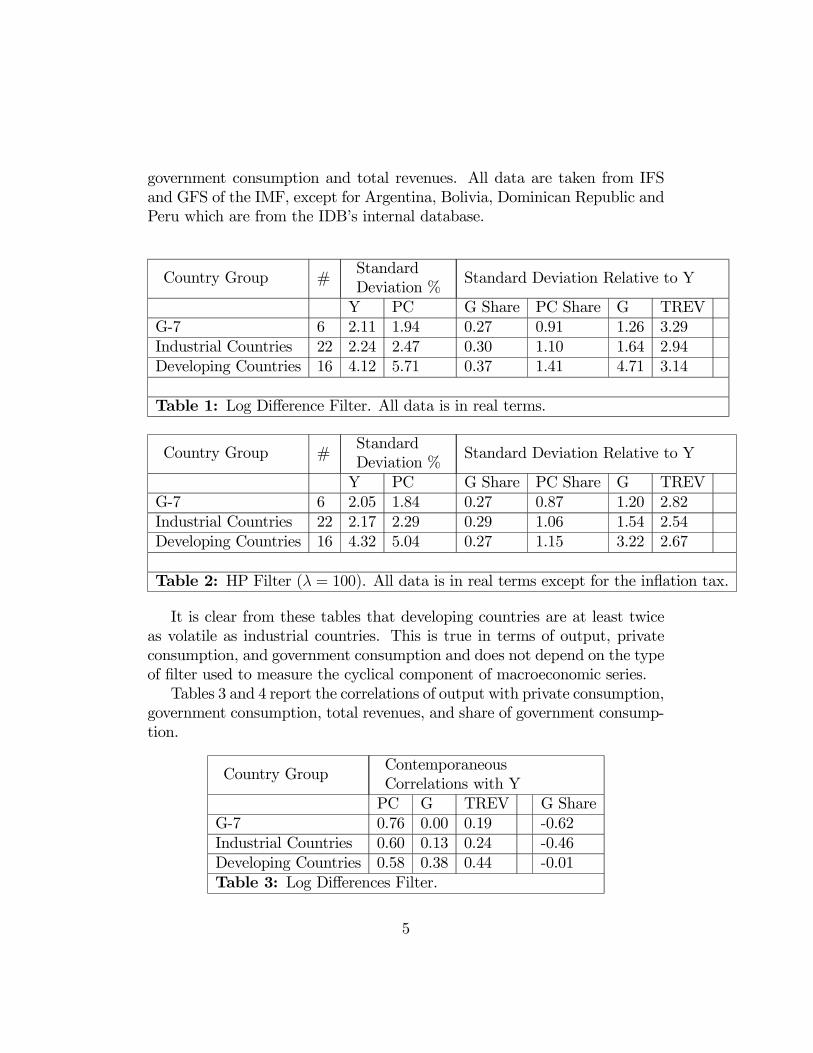
government consumption and total revenues. All data are taken from IFSand GFS of the IMF, except for Argentina, Bolivia, Dominican Republic andPeru which are from the IDB’s internal database.
Country Group #StandardDeviation %
Standard Deviation Relative to Y
Y PC G Share PC Share G TREVG-7 6 2.11 1.94 0.27 0.91 1.26 3.29Industrial Countries 22 2.24 2.47 0.30 1.10 1.64 2.94Developing Countries 16 4.12 5.71 0.37 1.41 4.71 3.14
Table 1: Log Difference Filter. All data is in real terms.
Country Group #StandardDeviation %
Standard Deviation Relative to Y
Y PC G Share PC Share G TREVG-7 6 2.05 1.84 0.27 0.87 1.20 2.82Industrial Countries 22 2.17 2.29 0.29 1.06 1.54 2.54Developing Countries 16 4.32 5.04 0.27 1.15 3.22 2.67
Table 2: HP Filter (λ = 100). All data is in real terms except for the inflation tax.
It is clear from these tables that developing countries are at least twiceas volatile as industrial countries. This is true in terms of output, privateconsumption, and government consumption and does not depend on the typeof filter used to measure the cyclical component of macroeconomic series.Tables 3 and 4 report the correlations of output with private consumption,
government consumption, total revenues, and share of government consump-tion.
Country GroupContemporaneousCorrelations with YPC G TREV G Share
G-7 0.76 0.00 0.19 -0.62Industrial Countries 0.60 0.13 0.24 -0.46Developing Countries 0.58 0.38 0.44 -0.01Table 3: Log Differences Filter.
5

Country GroupContemporaneousCorrelations with YPC G TREV G Share
G-7 0.82 -0.02 0.22 -0.64Industrial Countries 0.67 0.11 0.30 -0.48Developing Countries 0.64 0.46 0.56 -0.01Table 4: HP Filter (λ = 100).
For our purposes, the most notable facts from Tables and 3 and 4 are thefollowing:
1. The high positive correlation of output with government consump-tion for developing countries, as opposed to industrial countries or theGroup of Seven.
2. The high negative correlation of output with the share of governmentconsumption (in output) for the group of seven or industrial countriesas opposed to the almost null correlation for developing countries.
These facts do not depend on the type of filter that we use.
3 The complete markets case
Consider a small open economy inhabited by a large number of identically andinfinitively-lived agents with Von Neumann-Morgenstern utility functions.The economy is endowed with an exogenously-given and stochastic outputstream. There is a finite number of states of nature. Both the government andprivate agents have access to a complete set of Arrow-Debreu securities tradedin world capital markets. Denote by st = (s0, ..., st) the history of events upto and including period t. The probability as of time 0 of any particularhistory st is denoted by π(st). The initial realization, s0, is given. Let p(st+1)be the time t price in terms of consumption in period t (conditional on st)of an asset that promises to pay one unit in the event that st+1 is realized.
3.1 Households
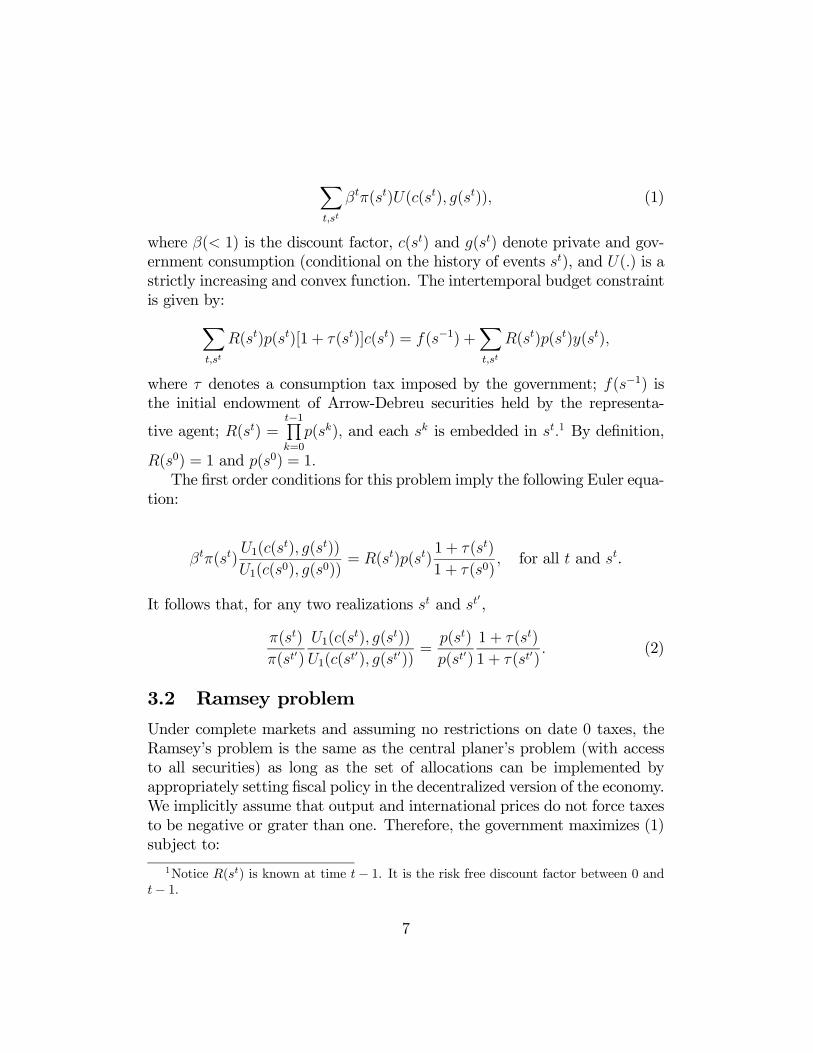
Since markets are complete, we can set up the agents’ decision problem asif all trade occurred in the first period (t = 0). The representative agent’slifetime utility is given by:
6
Xt,st
βtπ(st)U(c(st), g(st)), (1)
where β(< 1) is the discount factor, c(st) and g(st) denote private and gov-ernment consumption (conditional on the history of events st), and U(.) is astrictly increasing and convex function. The intertemporal budget constraintis given by:X
t,st
R(st)p(st)[1 + τ(st)]c(st) = f(s−1) +Xt,st
R(st)p(st)y(st),
where τ denotes a consumption tax imposed by the government; f(s−1) isthe initial endowment of Arrow-Debreu securities held by the representa-
tive agent; R(st) =t−1Qk=0
p(sk), and each sk is embedded in st.1 By definition,
R(s0) = 1 and p(s0) = 1.The first order conditions for this problem imply the following Euler equa-
tion:
βtπ(st)U1(c(s
t), g(st))
U1(c(s0), g(s0))= R(st)p(st)
1 + τ(st)
1 + τ(s0), for all t and st.
It follows that, for any two realizations st and st0,
π(st)
π(st0)
U1(c(st), g(st))
U1(c(st0), g(st0))
=p(st)
p(st0)
1 + τ(st)
1 + τ(st0). (2)
3.2 Ramsey problem
Under complete markets and assuming no restrictions on date 0 taxes, theRamsey’s problem is the same as the central planer’s problem (with accessto all securities) as long as the set of allocations can be implemented byappropriately setting fiscal policy in the decentralized version of the economy.We implicitly assume that output and international prices do not force taxesto be negative or grater than one. Therefore, the government maximizes (1)subject to:
1Notice R(st) is known at time t− 1. It is the risk free discount factor between 0 andt− 1.
7
Xt,st
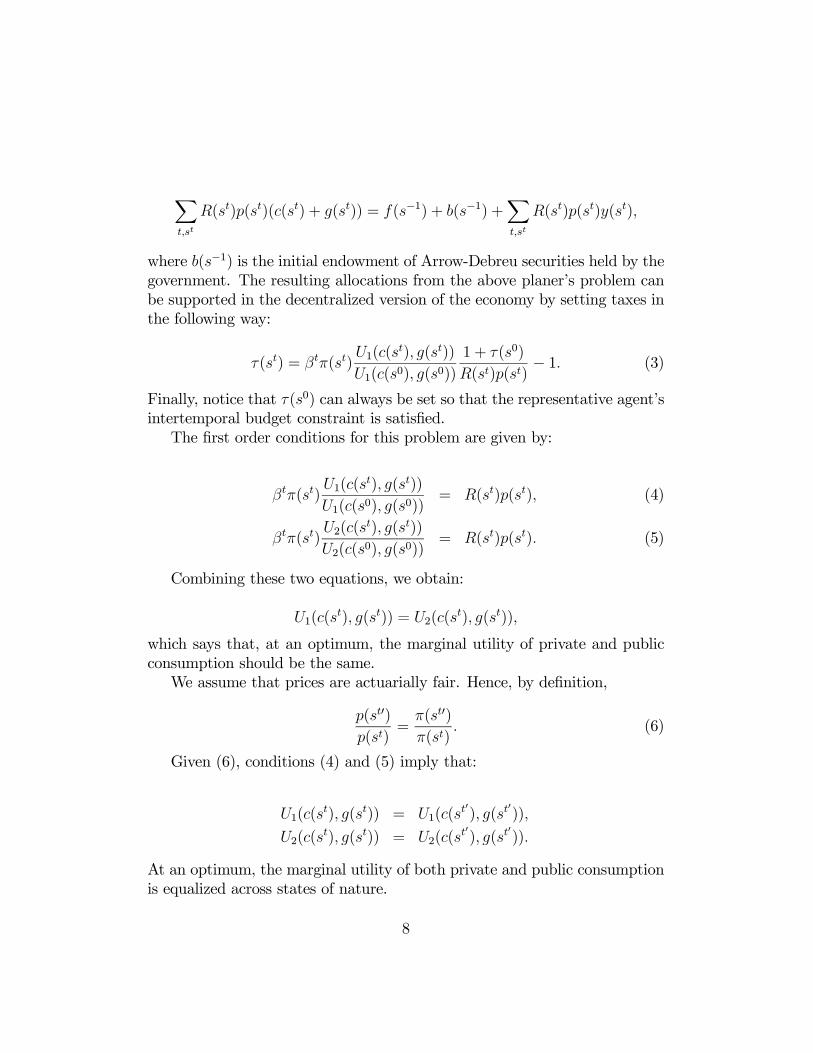
R(st)p(st)(c(st) + g(st)) = f(s−1) + b(s−1) +Xt,st
R(st)p(st)y(st),
where b(s−1) is the initial endowment of Arrow-Debreu securities held by thegovernment. The resulting allocations from the above planer’s problem canbe supported in the decentralized version of the economy by setting taxes inthe following way:
τ(st) = βtπ(st)U1(c(s
t), g(st))
U1(c(s0), g(s0))
1 + τ(s0)
R(st)p(st)− 1. (3)
Finally, notice that τ(s0) can always be set so that the representative agent’sintertemporal budget constraint is satisfied.The first order conditions for this problem are given by:
βtπ(st)U1(c(s
t), g(st))
U1(c(s0), g(s0))= R(st)p(st), (4)
βtπ(st)U2(c(s
t), g(st))
U2(c(s0), g(s0))= R(st)p(st). (5)
Combining these two equations, we obtain:
U1(c(st), g(st)) = U2(c(s
t), g(st)),
which says that, at an optimum, the marginal utility of private and publicconsumption should be the same.We assume that prices are actuarially fair. Hence, by definition,
p(st0)
p(st)=
π(st0)
π(st). (6)
Given (6), conditions (4) and (5) imply that:
U1(c(st), g(st)) = U1(c(s
t0), g(st0)),
U2(c(st), g(st)) = U2(c(s
t0), g(st0)).
At an optimum, the marginal utility of both private and public consumptionis equalized across states of nature.
8
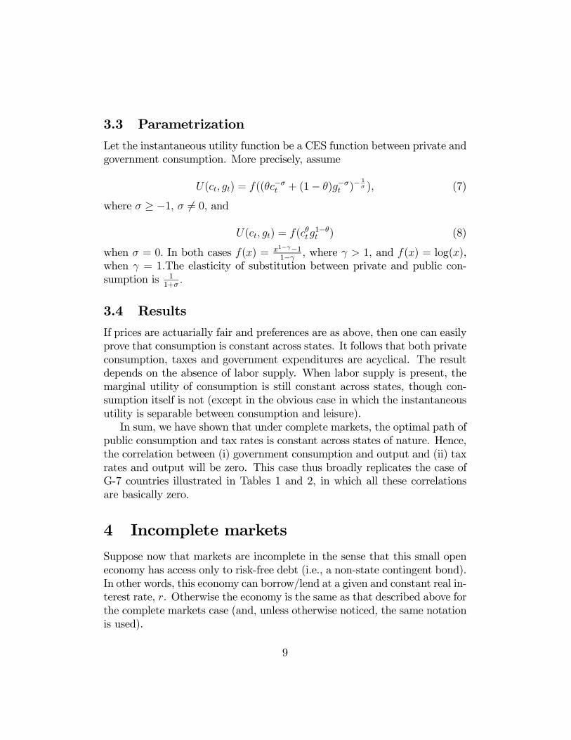
3.3 Parametrization
Let the instantaneous utility function be a CES function between private andgovernment consumption. More precisely, assume
U(ct, gt) = f((θc−σt + (1− θ)g−σt )−1σ ), (7)
where σ ≥ −1, σ 6= 0, and
U(ct, gt) = f(cθtg1−θt ) (8)
when σ = 0. In both cases f(x) = x1−γ−11−γ , where γ > 1, and f(x) = log(x),
when γ = 1.The elasticity of substitution between private and public con-sumption is 1
1+σ.
3.4 Results
If prices are actuarially fair and preferences are as above, then one can easilyprove that consumption is constant across states. It follows that both privateconsumption, taxes and government expenditures are acyclical. The resultdepends on the absence of labor supply. When labor supply is present, themarginal utility of consumption is still constant across states, though con-sumption itself is not (except in the obvious case in which the instantaneousutility is separable between consumption and leisure).In sum, we have shown that under complete markets, the optimal path of
public consumption and tax rates is constant across states of nature. Hence,the correlation between (i) government consumption and output and (ii) taxrates and output will be zero. This case thus broadly replicates the case ofG-7 countries illustrated in Tables 1 and 2, in which all these correlationsare basically zero.
4 Incomplete markets
Suppose now that markets are incomplete in the sense that this small openeconomy has access only to risk-free debt (i.e., a non-state contingent bond).In other words, this economy can borrow/lend at a given and constant real in-terest rate, r. Otherwise the economy is the same as that described above forthe complete markets case (and, unless otherwise noticed, the same notationis used).
9
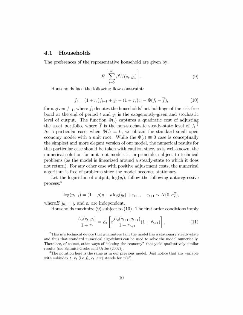
4.1 Households
The preferences of the representative household are given by:
E
" ∞Xt=0
βtU(ct, gt)
#. (9)
Households face the following flow constraint:
ft = (1 + rt)ft−1 + yt − (1 + τ t)ct − Φ(ft − f), (10)
for a given f−1, where ft denotes the households’ net holdings of the risk freebond at the end of period t and yt is the exogenously-given and stochasticlevel of output. The function Φ(.) captures a quadratic cost of adjustingthe asset portfolio, where f is the non-stochastic steady-state level of ft.2
As a particular case, when Φ(.) ≡ 0, we obtain the standard small openeconomy model with a unit root. While the Φ(.) ≡ 0 case is conceptuallythe simplest and more elegant version of our model, the numerical results forthis particular case should be taken with caution since, as is well-known, thenumerical solution for unit-root models is, in principle, subject to technicalproblems (as the model is linearized around a steady-state to which it doesnot return). For any other case with positive adjustment costs, the numericalalgorithm is free of problems since the model becomes stationary.Let the logarithm of output, log(yt), follow the following autoregressive
process:3
log(yt+1) = (1− ρ)y + ρ log(yt) + εt+1, εt+1 ∼ N(0, σ2),
whereE [yt] = y and εt are independent.Households maximize (9) subject to (10). The first order conditions imply
Uc(ct, gt)
1 + τ t= Et
∙βUc(ct+1, gt+1)
1 + τ t+1(1 + ert+1)¸ , (11)
2This is a technical device that guarantees taht the model has a stationary steady-stateand thus that standard numerical algorithms can be used to solve the model numerically.There are, of course, other ways of “closing the economy” that yield qualitatively similarresults (see Schmitt-Grohe and Uribe (2002)).
3The notation here is the same as in our previous model. Just notice that any variablewith subindex t, xt (i.e ft, ct, etc) stands for x(st).
10
limt→∞
ftt
Πi=0(1 + eri) = 0, (12)
where
1 + ert+1 ≡ 1 + rt+1
1 + Φ0(ft − f).
Condition (11) is the standard stochastic Euler equation.Notice that, from a computational point of view, the household’s problem
has a non-recursive structure since agents’ decisions rules for consumptionwill depend not only on the current state of the economy but also on allfuture taxes.
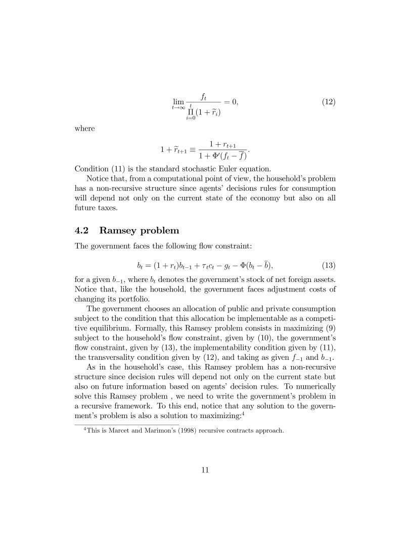
4.2 Ramsey problem
The government faces the following flow constraint:
bt = (1 + rt)bt−1 + τ tct − gt − Φ(bt − b), (13)
for a given b−1, where bt denotes the government’s stock of net foreign assets.Notice that, like the household, the government faces adjustment costs ofchanging its portfolio.The government chooses an allocation of public and private consumption
subject to the condition that this allocation be implementable as a competi-tive equilibrium. Formally, this Ramsey problem consists in maximizing (9)subject to the household’s flow constraint, given by (10), the government’sflow constraint, given by (13), the implementability condition given by (11),the transversality condition given by (12), and taking as given f−1 and b−1.As in the household’s case, this Ramsey problem has a non-recursive
structure since decision rules will depend not only on the current state butalso on future information based on agents’ decision rules. To numericallysolve this Ramsey problem , we need to write the government’s problem ina recursive framework. To this end, notice that any solution to the govern-ment’s problem is also a solution to maximizing:4
4This is Marcet and Marimon’s (1998) recursive contracts approach.
11

maxE
( ∞Xt=0
βt∙U(ct, gt) + µt[
Uc(ct, gt)
1 + τ t−Et(β
Uc(ct+1, gt+1)
1 + τ t+1(1 + ert+1))]¸) ,
subject to (10), (13), (11), and (12), and taking as given f−1 and b−1.Using the law of iterated expectations, one can easily show that the gov-
ernment’s objective function is equivalent to the following two equations:
E
" ∞Xt=0
βt∙U(ct, gt) + φt
Uc(ct, gt)
1 + τ t
¸#(14)
µt = (1 + ert)µt−1 + φt, µ−1 = 0 (15)
Hence, any solution to the original Ramsey problem must also be a solu-tion to the problem of maximizing (14) subject to (15), (10), (13), and (12),taking as given f−1 and b−1. This problem is recursive. The Lagrangian forthis problem is given by:
L = E∞Xt=0
βtU(ct, gt) + φtUc(ct, gt)
1 + τ t
+λt£ft − (1 + rt)ft−1 − yt + (1 + τ t)ct + Φ(ft − f)
¤+χt
£(bt − (1 + rt)bt−1 − τ tct + gt + Φ(bt − b)
¤+Ωt(
£µt − φt − µt−1(1 + ert)¤
In addition to (15), (10), and (13), the first order conditions are given by:
12
λt£1 + Φ0(ft − f)
¤= Et
∙βλt+1(1 + rt+1) + βΩt+1µt
∂ert+1∂ft
¸χt£1 + Φ0(bt − b)
¤= Et[βχt+1(1 + rt+1)]
Ωt = Et [βΩt+1(1 + ert+1)]φtUc(ct, gt)
(1 + τ t)2 + ctχt = λtct
Ug(ct, gt) + φtUcg(ct, gt)
(1 + τ t)+ χt = 0
Uc(ct, gt) + φtUcc(ct, gt)
(1 + τ t)+ λt(1 + τ t)− χtτ t = 0
Uc(ct, gt)
(1 + τ t)− Ωt = 0
The following additional conditions are sufficient for an optimum:
limt→∞
ftt
Πi=0(1 + eri) = 0
limt→∞
btt
Πi=0(1 + eri) = 0
limt→∞
µtt
Πi=0(1 + eri) = 0
f−1, b−1 given and µ−1 = 0
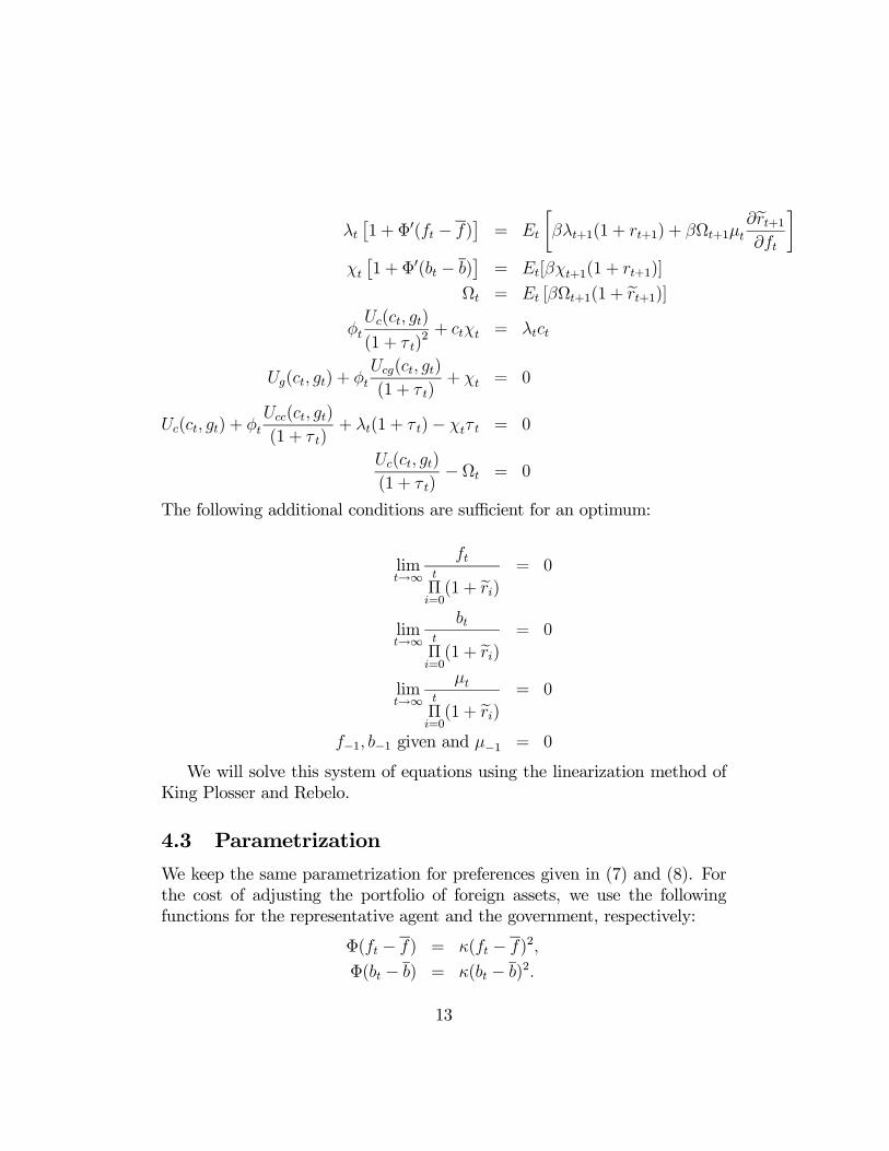
We will solve this system of equations using the linearization method ofKing Plosser and Rebelo.
4.3 Parametrization
We keep the same parametrization for preferences given in (7) and (8). Forthe cost of adjusting the portfolio of foreign assets, we use the followingfunctions for the representative agent and the government, respectively:
Φ(ft − f) = κ(ft − f)2,
Φ(bt − b) = κ(bt − b)2.
13
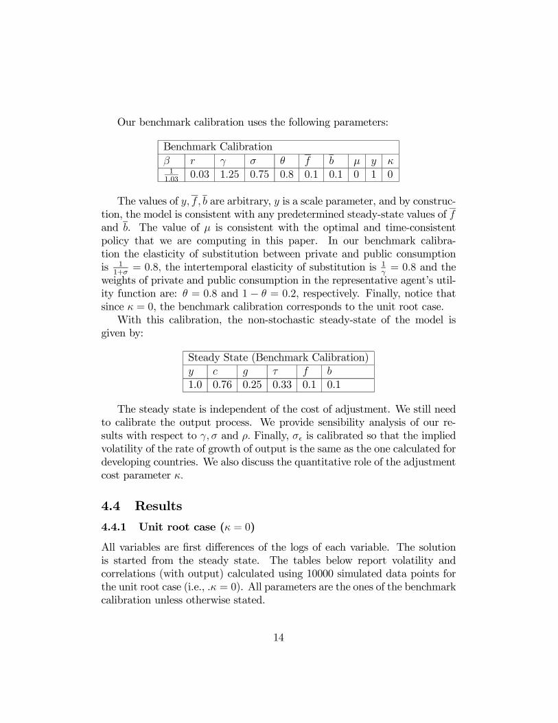
Our benchmark calibration uses the following parameters:
Benchmark Calibrationβ r γ σ θ f b µ y κ11.03
0.03 1.25 0.75 0.8 0.1 0.1 0 1 0
The values of y, f, b are arbitrary, y is a scale parameter, and by construc-tion, the model is consistent with any predetermined steady-state values of fand b. The value of µ is consistent with the optimal and time-consistentpolicy that we are computing in this paper. In our benchmark calibra-tion the elasticity of substitution between private and public consumptionis 1
1+σ= 0.8, the intertemporal elasticity of substitution is 1
γ= 0.8 and the
weights of private and public consumption in the representative agent’s util-ity function are: θ = 0.8 and 1 − θ = 0.2, respectively. Finally, notice thatsince κ = 0, the benchmark calibration corresponds to the unit root case.With this calibration, the non-stochastic steady-state of the model is
given by:
Steady State (Benchmark Calibration)y c g τ f b1.0 0.76 0.25 0.33 0.1 0.1
The steady state is independent of the cost of adjustment. We still needto calibrate the output process. We provide sensibility analysis of our re-sults with respect to γ, σ and ρ. Finally, σ is calibrated so that the impliedvolatility of the rate of growth of output is the same as the one calculated fordeveloping countries. We also discuss the quantitative role of the adjustmentcost parameter κ.
4.4 Results
4.4.1 Unit root case (κ = 0)
All variables are first differences of the logs of each variable. The solutionis started from the steady state. The tables below report volatility andcorrelations (with output) calculated using 10000 simulated data points forthe unit root case (i.e., .κ = 0). All parameters are the ones of the benchmarkcalibration unless otherwise stated.
14
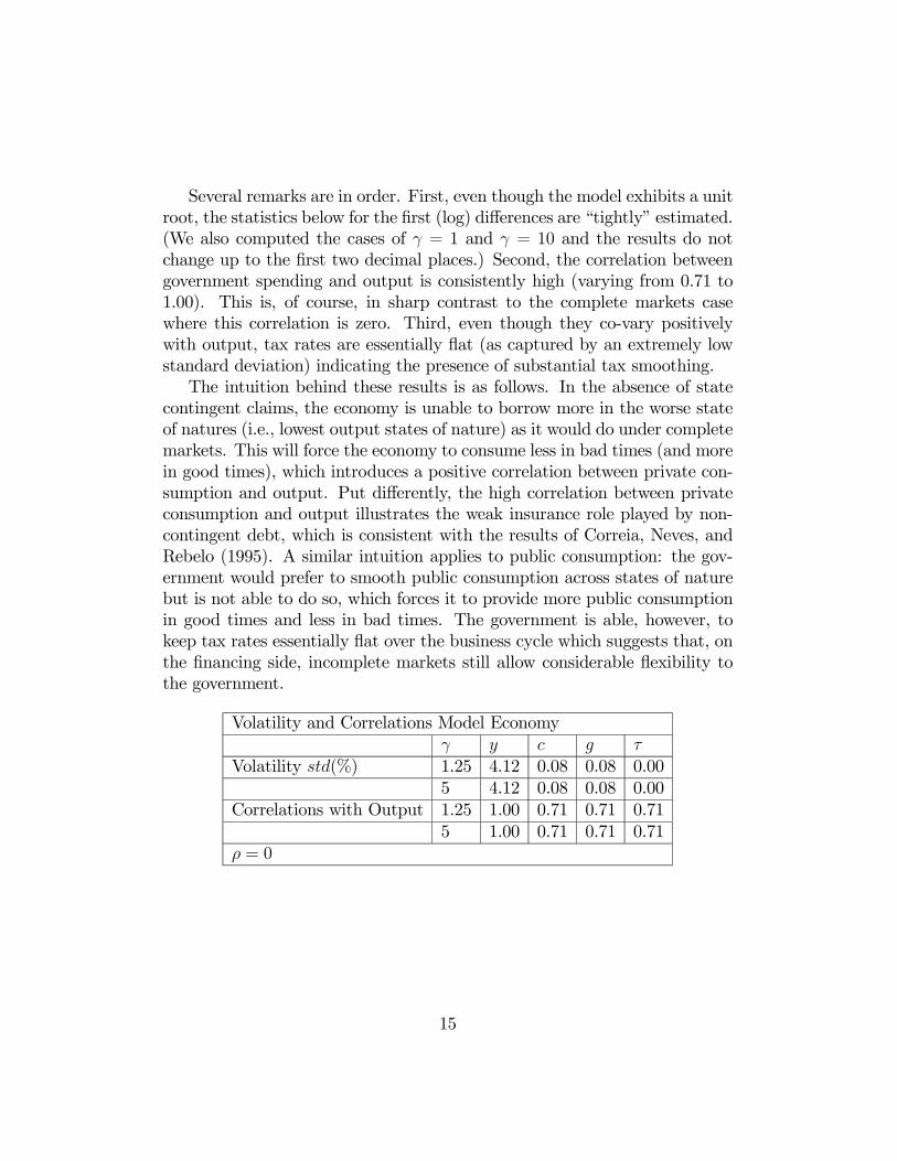
Several remarks are in order. First, even though the model exhibits a unitroot, the statistics below for the first (log) differences are “tightly” estimated.(We also computed the cases of γ = 1 and γ = 10 and the results do notchange up to the first two decimal places.) Second, the correlation betweengovernment spending and output is consistently high (varying from 0.71 to1.00). This is, of course, in sharp contrast to the complete markets casewhere this correlation is zero. Third, even though they co-vary positivelywith output, tax rates are essentially flat (as captured by an extremely lowstandard deviation) indicating the presence of substantial tax smoothing.The intuition behind these results is as follows. In the absence of state
contingent claims, the economy is unable to borrow more in the worse stateof natures (i.e., lowest output states of nature) as it would do under completemarkets. This will force the economy to consume less in bad times (and morein good times), which introduces a positive correlation between private con-sumption and output. Put differently, the high correlation between privateconsumption and output illustrates the weak insurance role played by non-contingent debt, which is consistent with the results of Correia, Neves, andRebelo (1995). A similar intuition applies to public consumption: the gov-ernment would prefer to smooth public consumption across states of naturebut is not able to do so, which forces it to provide more public consumptionin good times and less in bad times. The government is able, however, tokeep tax rates essentially flat over the business cycle which suggests that, onthe financing side, incomplete markets still allow considerable flexibility tothe government.
Volatility and Correlations Model Economyγ y c g τ
Volatility std(%) 1.25 4.12 0.08 0.08 0.005 4.12 0.08 0.08 0.00
Correlations with Output 1.25 1.00 0.71 0.71 0.715 1.00 0.71 0.71 0.71
ρ = 0
15
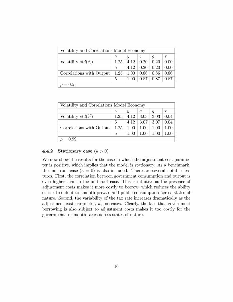
Volatility and Correlations Model Economyγ y c g τ
Volatility std(%) 1.25 4.12 0.20 0.20 0.005 4.12 0.20 0.20 0.00
Correlations with Output 1.25 1.00 0.86 0.86 0.865 1.00 0.87 0.87 0.87
ρ = 0.5
Volatility and Correlations Model Economyγ y c g τ
Volatility std(%) 1.25 4.12 3.03 3.03 0.045 4.12 3.07 3.07 0.04
Correlations with Output 1.25 1.00 1.00 1.00 1.005 1.00 1.00 1.00 1.00
ρ = 0.99
4.4.2 Stationary case (κ > 0)
We now show the results for the case in which the adjustment cost parame-ter is positive, which implies that the model is stationary. As a benchmark,the unit root case (κ = 0) is also included. There are several notable fea-tures. First, the correlation between government consumption and output iseven higher than in the unit root case. This is intuitive as the presence ofadjustment costs makes it more costly to borrow, which reduces the abilityof risk-free debt to smooth private and public consumption across states ofnature. Second, the variability of the tax rate increases dramatically as theadjustment cost parameter, κ, increases. Clearly, the fact that governmentborrowing is also subject to adjustment costs makes it too costly for thegovernment to smooth taxes across states of nature.
16
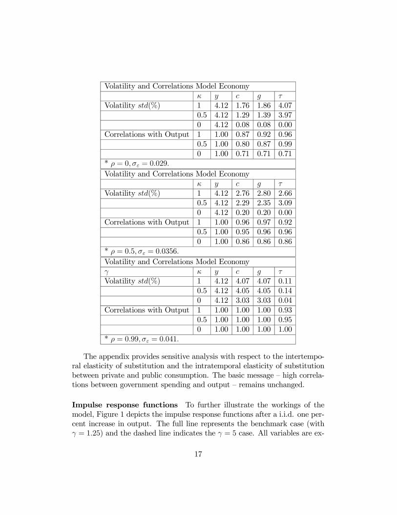
Volatility and Correlations Model Economyκ y c g τ
Volatility std(%) 1 4.12 1.76 1.86 4.070.5 4.12 1.29 1.39 3.970 4.12 0.08 0.08 0.00
Correlations with Output 1 1.00 0.87 0.92 0.960.5 1.00 0.80 0.87 0.990 1.00 0.71 0.71 0.71
* ρ = 0, σε = 0.029.Volatility and Correlations Model Economy
κ y c g τVolatility std(%) 1 4.12 2.76 2.80 2.66
0.5 4.12 2.29 2.35 3.090 4.12 0.20 0.20 0.00
Correlations with Output 1 1.00 0.96 0.97 0.920.5 1.00 0.95 0.96 0.960 1.00 0.86 0.86 0.86
* ρ = 0.5, σε = 0.0356.Volatility and Correlations Model Economyγ κ y c g τVolatility std(%) 1 4.12 4.07 4.07 0.11
0.5 4.12 4.05 4.05 0.140 4.12 3.03 3.03 0.04
Correlations with Output 1 1.00 1.00 1.00 0.930.5 1.00 1.00 1.00 0.950 1.00 1.00 1.00 1.00
* ρ = 0.99, σε = 0.041.
The appendix provides sensitive analysis with respect to the intertempo-ral elasticity of substitution and the intratemporal elasticity of substitutionbetween private and public consumption. The basic message — high correla-tions between government spending and output — remains unchanged.
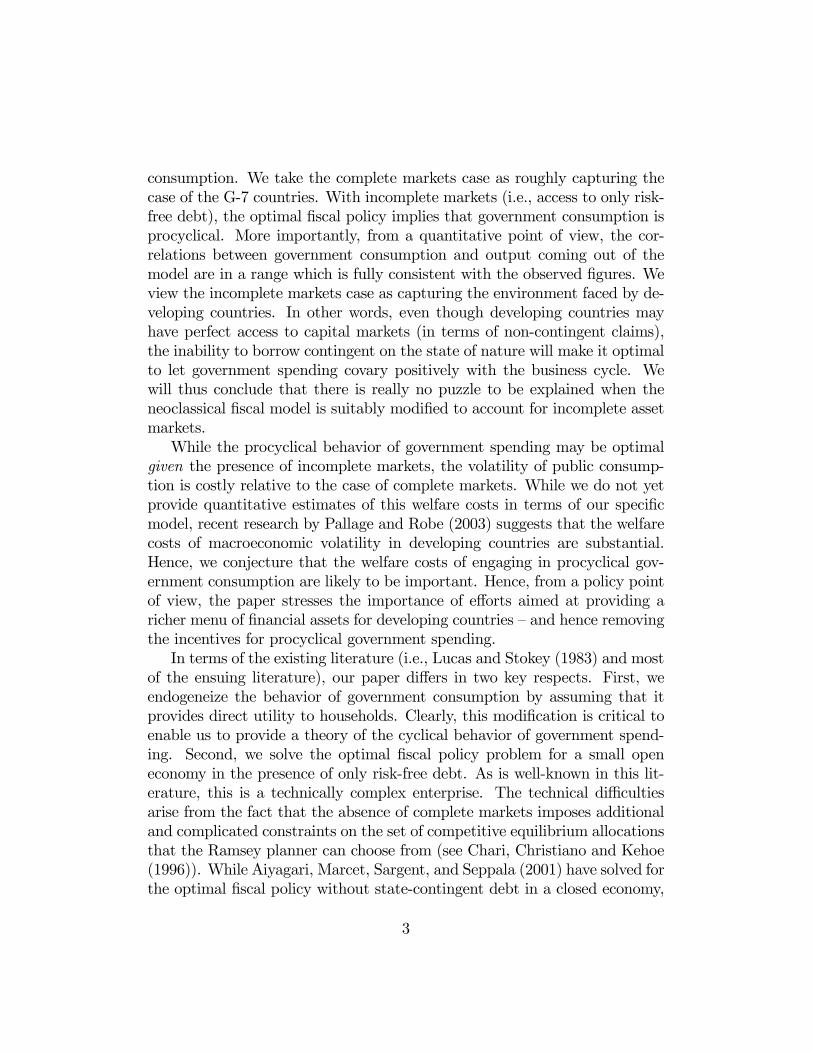
Impulse response functions To further illustrate the workings of themodel, Figure 1 depicts the impulse response functions after a i.i.d. one per-cent increase in output. The full line represents the benchmark case (withγ = 1.25) and the dashed line indicates the γ = 5 case. All variables are ex-
17
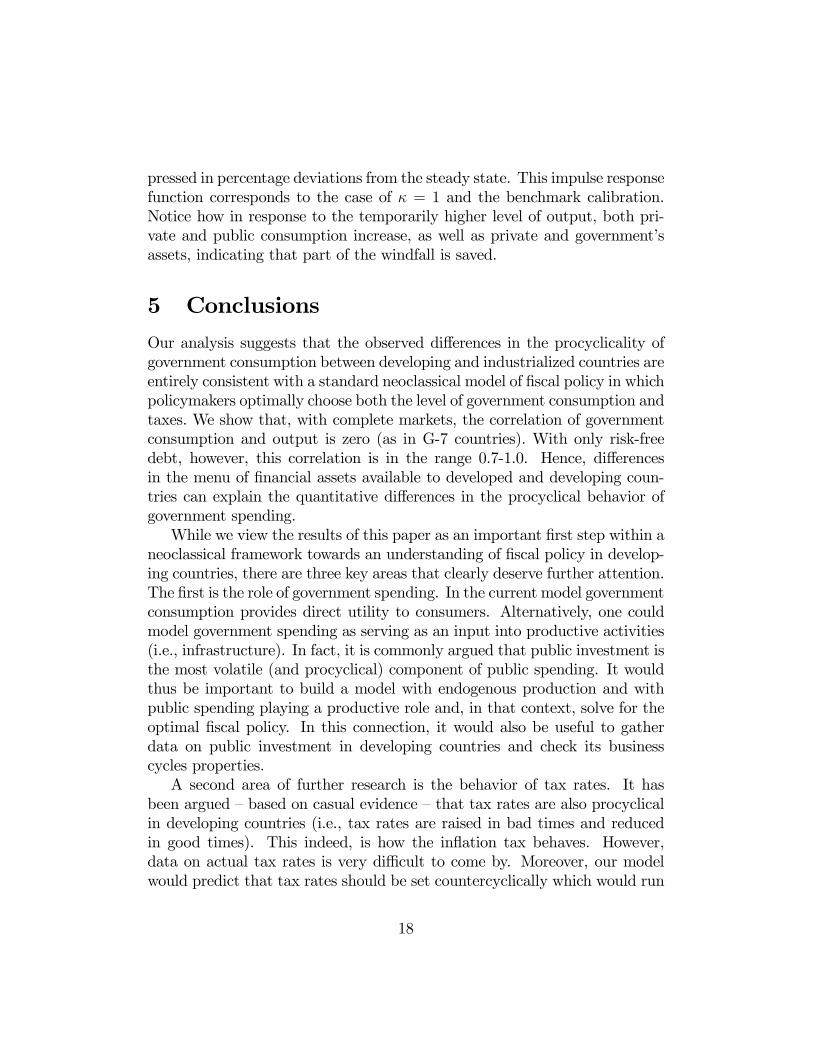
pressed in percentage deviations from the steady state. This impulse responsefunction corresponds to the case of κ = 1 and the benchmark calibration.Notice how in response to the temporarily higher level of output, both pri-vate and public consumption increase, as well as private and government’sassets, indicating that part of the windfall is saved.
5 Conclusions
Our analysis suggests that the observed differences in the procyclicality ofgovernment consumption between developing and industrialized countries areentirely consistent with a standard neoclassical model of fiscal policy in whichpolicymakers optimally choose both the level of government consumption andtaxes. We show that, with complete markets, the correlation of governmentconsumption and output is zero (as in G-7 countries). With only risk-freedebt, however, this correlation is in the range 0.7-1.0. Hence, differencesin the menu of financial assets available to developed and developing coun-tries can explain the quantitative differences in the procyclical behavior ofgovernment spending.While we view the results of this paper as an important first step within a
neoclassical framework towards an understanding of fiscal policy in develop-ing countries, there are three key areas that clearly deserve further attention.The first is the role of government spending. In the current model governmentconsumption provides direct utility to consumers. Alternatively, one couldmodel government spending as serving as an input into productive activities(i.e., infrastructure). In fact, it is commonly argued that public investment isthe most volatile (and procyclical) component of public spending. It wouldthus be important to build a model with endogenous production and withpublic spending playing a productive role and, in that context, solve for theoptimal fiscal policy. In this connection, it would also be useful to gatherdata on public investment in developing countries and check its businesscycles properties.A second area of further research is the behavior of tax rates. It has
been argued — based on casual evidence — that tax rates are also procyclicalin developing countries (i.e., tax rates are raised in bad times and reducedin good times). This indeed, is how the inflation tax behaves. However,data on actual tax rates is very difficult to come by. Moreover, our modelwould predict that tax rates should be set countercyclically which would run
18
0 50 1000
1
2
3
4b
0 50 1000
1
2
3
4f
0 50 1000
0.2
0.4
0.6
0.8
1y
0 50 100-1
-0.5
0
0.5
1
1.5tao
0 50 1000
0.2
0.4
0.6
0.8c
0 50 1000
0.2
0.4
0.6
0.8g
Figure 1: Impulse responses
19
counter to the conventional wisdom. We thus need to understand betterwhat are the stylized facts in this area and whether this is consistent or notwith the predictions of a neoclassical model.A third area would be to investigate an intermediate case of market in-
completeness and check that the procyclicality of government spending wouldfall in between the two extremes that we have analyzed. A potential candi-date would be to have a non-state contingent bond whose rate of return isstate contingent.
References
[1] Aiyagari, Rao, Albert Marcet, Thomas J. Sargent, and J. Seppala, “Op-timal Taxation without State-Contingent Debt” (mimeo, Stanford Uni-versity, 2001).
[2] Aizenman, Joshua, Michael Gavin, and Ricardo Hausmann, “OptimalTax Policy with Endogenous Borrowing Constraints,” NBER WorkingPaper No.5558 (1996).
[3] Ambler, Steve and Alain Paquet, “Fiscal Spending Shocks, EndogenousGovernment Spending, and the Real Business Cycle.” Journal of Eo-nomic Dynamics and Control. Vol 20 (1996), 237 - 256.
[4] Barro, Robert J., “On the Determination of Public Debt,” Journal ofPolitical Economy, Vol. 87 (1979), pp. 940-971.
[5] Braun, Miguel, “Why Is Fiscal Policy Procyclical in Developing Coun-tries?” (mimeo, Harvard University, 2001).
[6] Chari, V.V., Lawrence J. Christiano, and Patrick J. Kehoe, “PolicyAnalysis in Business Cycles Models,” in Thomas Cooley, ed., Frontiersof Business Cycle Research (New Jersey: Princeton University Press).
[7] Correia, Isabel, J. Neves and Sergio Rebelo,“Business Cycles in a SmallOpen Economy.” European Economic Review, Vol 39 (1995), pp. 1089-1113
[8] Den Haan, Wouter J., and Albert Marcet, “Solving the StochasticGrowth Model by Parameterizing Expectations.” Journal of Businessand Economic Statistics, Vol. 8 (1990), pp. 31-34.
20
[9] Gavin, Michael, and Roberto Perotti, “Fiscal Policy in Latin America,”NBER Macroeconomics Annual (Cambridge, Mass.: MIT Press, 1997),pp. 11-61.
[10] Judd, K. 1992. “ProjectionMethods for Solving Aggregate GrowthMod-els.” Journal of Economic Theory, Vol. 58 (1992), pp. 410-452.
[11] Lane, Philip R., “The Cyclical Behaviour of Fiscal Policy: Evidencefrom the OECD” (mimeo, Trinity College, Dublin, 2001).
[12] Lucas, Robert E., Jr, and Nancy L. Stokey, “Optimal Fiscal and Mone-tary Policy in an Economy without Capital,” Journal of Monetary Eco-nomics, Vol. 12 (1983), pp. 55-93.
[13] Lutkepohl, Helmut. Introduction to Multiple Time Series. Second Edi-tion. Springer Verlag (1993). .
[14] Marcet, Albert, and Ramon Marimon, “Recursive Contracts” (mimeo,Pompeu Fabra University, 1998).
[15] Stein, Ernesto, Ernesto Talvi, and Alejandro Grisanti, “InstitutionalArrangements and Fiscal Performance: The Latin American Experi-ence,” in James M. Poterba and Jurgen Von Hagen, eds., Fiscal Insti-tutions and Fiscal Performance (Chicago: University of Chicago Press,1999).
[16] Talvi, Ernesto, and Carlos A. Végh,“Tax Base Variability and Procycli-cal Fiscal Policy,” NBER Working Paper No. 7499 (2000).
[17] Tornell, Aaron and Philip R. Lane, “The Voracity Effect,” AmericanEconomic Review, Vol. 89 (1999), pp. 22-46.
A Sensitivity analysis: intertemporal elastic-ity of substitution
³11+γ
´All variables are first differences of the logs of each variable. The solutionis started from the steady state. The following tables report some statisticscalculated using 10000 simulated data points. All parameters are the ones ofthe benchmark calibration unless otherwise stated. We set κ = 1.
21
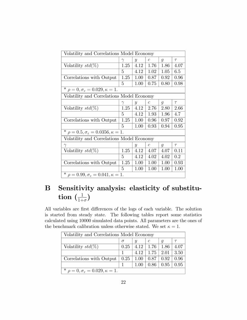
Volatility and Correlations Model Economyγ y c g τ
Volatility std(%) 1.25 4.12 1.76 1.86 4.075 4.12 1.02 1.05 6.5
Correlations with Output 1.25 1.00 0.87 0.92 0.965 1.00 0.75 0.80 0.98
* ρ = 0, σε = 0.029, κ = 1.Volatility and Correlations Model Economy
γ y c g τVolatility std(%) 1.25 4.12 2.76 2.80 2.66
5 4.12 1.93 1.96 4.7Correlations with Output 1.25 1.00 0.96 0.97 0.92
5 1.00 0.93 0.94 0.95* ρ = 0.5, σε = 0.0356, κ = 1.Volatility and Correlations Model Economyγ y c g τVolatility std(%) 1.25 4.12 4.07 4.07 0.11
5 4.12 4.02 4.02 0.2Correlations with Output 1.25 1.00 1.00 1.00 0.93
5 1.00 1.00 1.00 1.00* ρ = 0.99, σε = 0.041, κ = 1.
B Sensitivity analysis: elasticity of substitu-tion ( 1
1+σ)
All variables are first differences of the logs of each variable. The solutionis started from steady state. The following tables report some statisticscalculated using 10000 simulated data points. All parameters are the ones ofthe benchmark calibration unless otherwise stated. We set κ = 1.
Volatility and Correlations Model Economyσ y c g τ
Volatility std(%) 0.25 4.12 1.76 1.86 4.071 4.12 1.75 2.01 3.50
Correlations with Output 0.25 1.00 0.87 0.92 0.961 1.00 0.86 0.95 0.95
* ρ = 0, σε = 0.029, κ = 1.
22
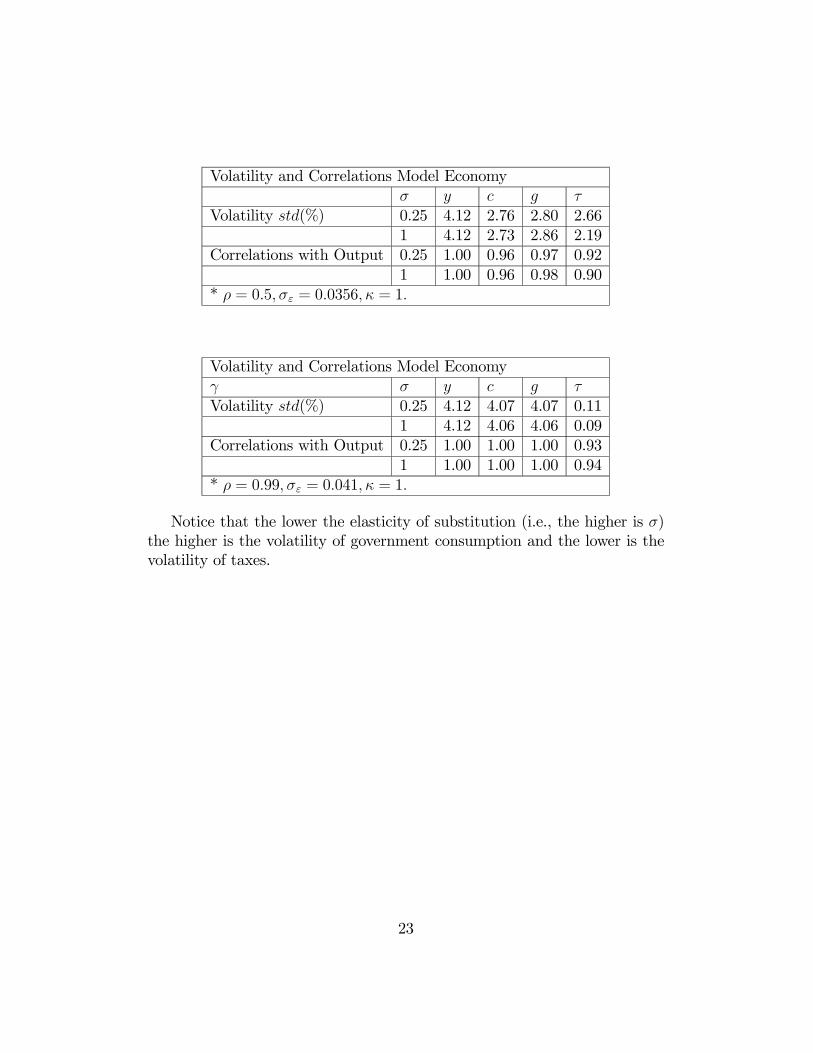
Volatility and Correlations Model Economyσ y c g τ
Volatility std(%) 0.25 4.12 2.76 2.80 2.661 4.12 2.73 2.86 2.19
Correlations with Output 0.25 1.00 0.96 0.97 0.921 1.00 0.96 0.98 0.90
* ρ = 0.5, σε = 0.0356, κ = 1.
Volatility and Correlations Model Economyγ σ y c g τVolatility std(%) 0.25 4.12 4.07 4.07 0.11
1 4.12 4.06 4.06 0.09Correlations with Output 0.25 1.00 1.00 1.00 0.93
1 1.00 1.00 1.00 0.94* ρ = 0.99, σε = 0.041, κ = 1.
Notice that the lower the elasticity of substitution (i.e., the higher is σ)the higher is the volatility of government consumption and the lower is thevolatility of taxes.
23