Discussion Paper No. 1009

PRODUCT DIFFERENTIATION AND ENTRY TIMING

IN A CONTINUOUS-TIME SPATIAL COMPETITION MODEL

WITH VERTICAL RELATIONS

Takeshi Ebina Noriaki Matsushima

August 2017

The Institute of Social and Economic Research Osaka University

6-1 Mihogaoka, Ibaraki, Osaka 567-0047, Japan

Product differentiation and entry timing in a

continuous-time spatial competition model with

vertical relations∗

Takeshi Ebina†

Institute of Social Sciences, Shinshu University

Noriaki Matsushima‡

Institute of Social and Economic Research, Osaka University

August 17, 2017

Abstract

We study the entry timing and location decisions of two exclusive buyer–supplierrelationships in a continuous-time spatial competition model. In each relationship,the firms determine their entry timing and location, and negotiate a wholesale pricethrough Nash bargaining. Then, the downstream firm immediately determines its retailprice. Our findings are as follows. Ordinarily, if the supplier of the first entrant (calledthe leader pair) has strong bargaining power, the equilibrium location of the leaderwill be closer to the center, inducing a delay in entry by the second entrant (called thefollower pair). This delay implies the stronger bargaining power of the supplier in theleader pair can also benefit the buyer of the pair. The location of the leader pair canchange non-monotonically with an increase in the supplier’s bargaining power, whichhas a substantial impact on the entry timing of the follower pair. However, the greaterthe bargaining power of the supplier in the follower pair, the closer the leader pair willbe to the edge. This implies that having greater bargaining power will enhance theprofitability of the supplier in the follower pair.

Keywords: Entry timing; Hotelling model; Vertical relations; Continuous-time model; NashbargainingJEL codes: C71, L11, L13, R32.

∗The authors gratefully acknowledge financial support from a Grant-in-Aid for Basic Research (15H03349,15H05728, 17H00984) and Young Scientists (15K17047) from the Japan Society for the Promotion of Scienceand the MEXT. We also thank seminar participants at Shinshu University for helpful comments. Needlessto say, we are responsible for any remaining errors.

†Institute of Social Sciences, Shinshu University, 3-1-1, Asahi, Matsumoto, Nagano, Japan. Phone: (81)-4-8021-7663. Fax: (81)-4-8021-7654. E-mail: ebina@shinshu-u.ac.jp

‡Institute of Social and Economic Research, Osaka University, Mihogaoka 6-1, Ibaraki, Osaka, Japan.Phone: (81)-6-6879-8571. Fax: (81)-6-6879-8583. E-mail: nmatsush@iser.osaka-u.ac.jp

1

1 Introduction

When firms face situations in which markets are growing, as in new product markets and

newly developed cities, the timing of entry and product positioning are important strategic

issues. For instance, mobile phone services have been growing in most countries since they

were first introduced in 1981 in Scandinavia; and for some countries, the penetration levels

of mobile phones have already reached more than 100% (Peres et al., 2010). In addition,

“the massive penetration of mobile telephony is not exceptional —many commonly used

products and services, such as DVDs, personal computers, digital cameras, online banking,

and the Internet, were unknown to consumers three decades ago” (Peres et al., 2010, p.91).

Naturally, companies in these industries consider product positions and entry decisions when

they launch new products. In addition, in the context of retailing, many leading retailers in

developed countries have launched stores in countries that are in different stages of economic

development (Reinartz et al., 2011). In particular, in emerging countries, including the

BRIC countries, Mexico, Poland, and South Africa, “the total population [...] considerably

exceeds the population of developed countries, making these regions particularly attractive

for mature market-based retailers and retailing innovations that are responsive to the dis-

tinctive characteristics of these markets” (Reinartz et al., 2011, p.S55). In this context, the

profitability of these retailers is significantly influenced by geographical distances and the

location choices of rivals in each region.1

Manufacturers/franchisors usually sell their products through independent downstream

representatives/franchisees; that is, vertical relations are often observed in contexts such as

1 Several empirical studies show that geographical proximity influences the pricing decisions of retailers

(Bronnenberg and Mahajan, 2001; Zhu and Singh, 2009; Cleeren et al., 2010; Orhun, 2013). In addi-

tion, many studies have empirically investigated how positioning strategies influence firm profitability (e.g.,

Thomadsen, 2007; Draganska et al., 2009; Hwang et al., 2010).

2

manufacturers and retail representatives, franchisors and franchisees, and so on.2 In this con-

text, several papers emphasize that large nationwide retailers tend to have strong bargaining

power over their upstream trading partners, enabling them to be highly competitive in re-

tail markets (Geylani et al., 2007; Inderst and Shaffer, 2007, 2009). In other words, strong

bargaining power over trading partners is recognized as a source of competitiveness. In sum-

mary, when examining the growth of markets and vertical relations, we need to consider

firms’ product positioning and entry timing.

In line with the literature on positioning strategies and product differentiation (in mar-

keting, Wernerfelt, 1986; Hauser, 1988; Moorthy, 1988; Desai, 2001; Kuksov, 2004; Sajeesh

and Raju, 2010, among others; in economics, d’Aspremont et al., 1979; Tabuchi and Thisse,

1995; Kim and Serfes, 2006; Matsumura and Matsushima, 2009; Sajeesh, 2016, among oth-

ers), we investigate how market growth influences product positioning/differentiation in a

continuous-time spatial competition model with entry timing decisions and vertical relations.

In the context of economics, marketing, and related fields, with the exception of Lambertini

(2002), Ebina et al. (2015), and Ebina et al. (2017),3 no studies have investigated product

positioning strategies using continuous-time Hotelling-type spatial competition models with

market growth and entry timing. However, several related studies do use Hotelling models

to investigate the sequential entry of firms (e.g., Gotz, 2005, Loertscher and Muehlheusser,

2011) and buyer–supplier relations (e.g., Brekke and Straume, 2004; Matsushima, 2004,

2009; Erkal, 2007, Geylani et al., 2007; Liu and Tyagi, 2011; Matsushima and Miyaoka,

2015; Matsushima and Pan, 2016).

2 Several recent studies investigate the objectives of retailers and their increased power in channels

(Dobson and Waterson, 1997; Chen, 2003; Raju and Zhang, 2005; Dukes et al., 2006). In addition, in the

context of outsourcing by downstream firms, several studies investigate the interactions between sourcing

modes and profitability (Liu and Tyagi, 2011; Matsushima and Pan, 2016).3 Using a non-spatial dynamic duopoly model with exclusive vertical relations, Alipranti et al. (2015)

investigate the timing of technology adoption and contract types (linear pricing and two-part tariffs).

3

This study substantially extends the work of Ebina et al. (2015) by incorporating two

pairs of an upstream supplier/franchisor and a downstream buyer/franchisee in their model.

Ebina et al. (2015) discuss endogenous decisions on locations and entry-timing in a Hotelling

duopoly model with market growth.4 Here, we investigate how upstream suppliers’ bargain-

ing power over downstream buyers influences the locations of the two pairs, the timing of

entry by the follower pair, and the value of each firm.

Our findings are as follows. Ordinarily, if the supplier in a leader pair has stronger

bargaining power (denoted as β1), this induces the pair to locate closer to the center, and the

follower pair to enter the market later. This implies that the stronger bargaining power of the

supplier can also benefit the downstream buyer. That is, it might be better for a downstream

buyer to weaken its bargaining position over its trading supplier. In reality, there are several

examples in which buyers encourage suppliers to organize collective associations, even though

this would weaken the buyers’ bargaining power (e.g., the Carrefour case in Raynaud et al.

(2009, pp.851–2)). In addition, there can be a non-monotonic relation between β1 and the

leader pair’s location. More specifically, the equilibrium location of the leader pair can

jump significantly with an increase in β1, which delays the entry timing of the follower pair

substantially. On the other hand, an increase in the bargaining power of the supplier in the

follower pair induces the leader pair to locate closer to the edge, which facilitates earlier

entry by the follower pair. This implies that when an upstream manufacturer tries to enter a

newly growing market with its downstream representative, maintaining its bargaining power

over its representative is quite important.

The remainder of the paper organized as follows. Section 2 provides the model setting,

and Section 3 describes the results of the model. Section 4 provides numerical analyses of

4 Ebina et al. (2017) provide another major extension to the work of Ebina et al. (2015) by incorporating

market-size uncertainty with Brownian motion in the setting of Ebina et al. (2015). However, the direction

of this extension is quite different to ours.

4

the model. Then, Section 5 discusses the relation between our study and that of Ebina et al.

(2015), as well as the case in which the bargaining power in each pair is symmetric. Section

6 concludes the paper, and Section 7 is the Appendix.

2 Model

There are two competing upstream firms U1 and U2. Upstream firm Ui forms a vertical group

with a downstream firm Di (i = 1, 2). Thus, there are four firms: two upstream firms U1 and

U2, and two downstream firms D1 and D2. In group i, Ui and Di negotiate a wholesale price

wit, paid from Di to Ui at time t. The negotiation is based on the standard Nash bargaining

(Muthoo, 1999). Here, βi ∈ [0, 1] denotes the bargaining power of Ui.

There is a mass of consumers uniformly distributed on the line segment [0, 1]. The size

of this mass is exp(αt), where α is the growth rate of the size (market size). The utility of

the consumer at point x ∈ [0, 1] at time t ∈ [0,∞) is given by

ut(x;x1, x2, p1t, p2t) =

u− p1t − c(x1 − x)2 if purchased from firm D1,

u− p2t − c(x2 − x)2 if purchased from firm D2,

0 otherwise,

(1)

where u > 0 denotes the gross surplus that a consumer at point x ∈ [0, 1] enjoys from

purchasing the good, pit is the price of Di at time t, and c > 0 is a parameter describing

the level of transportation cost or product differentiation.5 From (1), the consumer who is

indifferent between purchasing from D1 and D2 is x = [p2t − p1t + c(x22 − x2

1)]/[2c(x2 − x1)].

We assume that u is so large that all consumers purchase one unit of the product from one

of the firms. More specifically, we assume the following inequality:

Assumption 1 u > m+ 3c.

5 We consider a situation in which the population of consumers at time t is N exp(αt), which we normalize

to N = 1. Therefore, our interpretation is that α corresponds to the increasing rate of population and is

called the market growth rate. This interpretation is the same as that of Ebina et al. (2015). The validity

of this assumption under the Hotelling model is explained in Footnote 7 of their study.

5

The sequence of entries is as follows: Group 1 is the leader pair, who enter immediately

at T1 = 0. Group 2 is the follower pair, who enter at time T2 ∈ (0,∞), which is determined

endogenously later. Firm Di incurs an entry cost Fi(Ti), which is evaluated at time 0 and

decreasing in Ti. The game analyzed is an infinite-horizon game.

In group 1, U1 determines the group’s location x1 at time T1 = 0. We assume (without

loss of generality) that x1 ≤ 1/2 holds in equilibrium. After entry, w1t is determined through

Nash bargaining between D1 and U1, and then D1 sets its price p1t at t ∈ [τ, τ + dτ). Group

1 becomes the monopoly, and can repeat the bargaining and pricing process whenever group

2 is out of the market.

In group 2, U2 offers a contract (T2, x2) to D2 unilaterally. This implies that U2 is in a

strong position over D2 only in terms of the entry timing.6 Note that we assume that the

follower group enters if and only if entry is just acceptable for D2, although we can derive

similar results under a different criterion for the entry decision, which is assumed in Ebina

et al. (2015).7

After entry, competition between the groups occurs. Here, w1t and w2t are determined

simultaneously through Nash bargaining. Observing the negotiation outcomes, D1 and D2

simultaneously set their prices p1t and p2t at t ∈ [τ, τ + dτ).

The total profits of the upstream (V1 and V2) and downstream (v1 and v2) firms of groups

1 and 2 (the leader and the follower pairs, respectively) are given by

V1(T2, x1, x2, p1t, p2t, w1t) =

∫ T2

0

∫ 1

0

[w1t −m]e−(r−α)tdxdt+

∫ ∞

T2

∫ x

0

[w1t −m]e−(r−α)tdxdt,

(2)

6 This assumption is suitable to situations in which U2 is able to select one of many potential downstream

agents. However, U2 then faces a lock-in after signing the contract with D2, owing to the necessary coordi-

nation with D2 for production, giving some bargaining power to D2.7 Other than incorporating a negotiation in each group and a unilateral offer of the contract (T2, x2) by

U2 to D2, the basic timing structure is the same as that of Ebina et al. (2015). However, our main results

hold even under a different criterion for the entry decision. We discuss this point in Section 5.1.

6

v1(T2, x1, x2, p1t, p2t, w1t) =

∫ T2

0

∫ 1

0

[p1t − w1t]e−(r−α)tdxdt

+

∫ ∞

T2

∫ x

0

[p1t − w1t]e−(r−α)tdxdt− F1(0), (3)

and

V2(T2, x1, x2, p1t, p2t, w2t) =

∫ ∞

T2

∫ 1

x

[w2t −m]e−(r−α)tdxdt, (4)

v2(T2, x1, x2, p1t, p2t, w2t) =

∫ ∞

T2

∫ 1

x

[p2t(x; x1, x2, p1t)− w2t]e−(r−α)tdxdt− F2(T2), (5)

where m and r denote the marginal cost of each upstream firm and the interest rate, re-

spectively. We assume that r > α to ensure that the follower enters within a finite time

frame.8

With respect to the bargaining power of group 1, we make the following assumption:

Assumption 2 β1 ∈ (0, (u−m− 3c)/(u−m− c)).

This assumption ensures that the monopoly outcome of group 1 at each t ∈ [0, T2) has an

interior solution. With respect to F2, we also make the following assumption:

Assumption 3 (i) Fi(Ti) = Fi exp(−rTi). (ii) F2 > [c(2+β1)2(2−β2)

2]/[(r−α)(4−β1β2)2].

Assumption 3 (i) is made to explicitly obtain an outcome for the subgame perfect Nash

equilibrium, and is the same as that in Ebina et al. (2015).9 Assumption 3 (ii) ensures that

8 If r ≤ α, the integral of Equation (4) could be made indefinitely larger by choosing a larger time T2.

Thus, waiting longer would always be a better strategy, and the optimum would not exist.9 We adopt a setting where α represents the increasing rate of population, because we consider that this

interpretation is more natural and valid under a Hotelling location model. However, many studies consider

that α represents a cost-reducing rate when firms adopt a new technology, and assume Fi = exp(−(r−α)Ti).

If we modify our interpretation (growing market) to that of technology improvement, our main results do

not change. Here, we can make a similar argument to that explained in the Appendix of Ebina et al. (2015,

p.912).

7

group 2 enters at a positive time T2(> 0), and that sequential entry always occurs. This

allows us to avoid simultaneous entry at time 0 and to focus on sequential entry.10

The game proceeds as follows: At T1 = 0, U1 in group 1 determines the location of group

1, x1, in order to maximize its own total profit. Observing x1, and to maximize its own

total profit, U2 offers contract (T2, x2) to D2. At each instance t ∈ [τ, τ + dτ), and knowing

whether group 2 is active, group i determines wit through Nash bargaining between Ui and

Di, if the group is active. Finally, Di sets its price pit.

3 Equilibrium

We derive the price outcome in the subgame perfect Nash equilibrium in Section 3.1, the

timing and the location outcomes of group 2 in Section 3.2, the location outcome of group

1 in Section 3.3, and the outcomes of the subgame perfect Nash equilibrium in Section 3.4.

3.1 Price

First, we consider the problem of prices at each t ∈ [τ, τ + dτ), before and after the entry of

group 2, given x1, x2, and T2. Then, we derive the local profits of U1, U2, D1, and D2 at each

t ∈ [τ, τ + dτ). Next, we provide the relations between the local profits and the bargaining

power parameters, β1 and β2, in Remarks 1 to 3. The three remarks will be helpful to

understand the intuition behind our main results shown in this and the next sections.

First, we consider the subgame after group 2 enters, that is, the subgame at t ∈ [T2,∞).

10 If simultaneous entry occurs, our model reverts to the standard location-price model with a vertical

relationship. Then, an equilibrium location pattern simply becomes the maximum differentiation. For more

detail, see Brekke and Straume (2004).

8

Given w1t and w2t at t ∈ [T2,∞), the profits of the downstream firms are

π1t(p1t, p2t; x1, x2, w1t) = (p1t − w1t)x,

π2t(p1t, p2t; x1, x2, w1t) = (p2t − w2t)(1− x).

Solving the first-order conditions of the downstream firms, we have the following instanta-

neous prices:

p1t(w1t, w2t;x1, x2) =2w1t + w2t + c (x2 − x1) (2 + x1 + x2)

3, (6)

p2t(w1t, w2t;x1, x2) =w1t + 2w2t + c (x2 − x1) (4− x1 − x2)

3. (7)

Substituting these into the profits of the firms and x, we have

π1t(w1t, w2t, x1, x2) =(w2t − w1t + c(x2 − x1)(2 + x1 + x2))

2

18c(x2 − x1),

π2t(w1t, w2t, x1, x2) =(w1t − w2t + c(x2 − x1)(4− x1 − x2))

2

18c(x2 − x1),

Π1t(w1t, w2t, x1, x2) =(w1t −m)(w2t − w1t + c(x2 − x1)(2 + x1 + x2))

6c(x2 − x1),

Π2t(w1t, w2t, x1, x2) =(w2t −m)(w1t − w2t + c(x2 − x1)(4− x1 − x2))

6c(x2 − x1),

x(w1t, w2t, x1, x2) =2 + x1 + x2

6+

w2t − w1t

6c(x2 − x1).

Next, we consider the bargaining problems in the vertical groups. Substituting the profits

into the objective functions of the bargaining problems in the vertical chains, Ω1t and Ω2t,

we have

Ω1t(w1t, w2t;x1, x2) = [Π1t(w1t, w2t, x1, x2)]β1 [π1t(w1t, w2t, x1, x2)]

1−β1 ,

Ω2t(w1t, w2t;x1, x2) = [Π2t(w1t, w2t, x1, x2)]β2 [π2t(w1t, w2t, x1, x2)]

1−β2 .

Each vertical group i determines wi to maximize Ωit. Solving the maximization problems of

9

the groups, we have

w1t(x1, x2) = m+cβ1 (x2 − x1) [2(2 + x1 + x2) + (4− x1 − x2)β2]

4− β1β2

(≡ wD1 (x1, x2)),

w2t(x1, x2) = m+cβ2 (x2 − x1) [2(4− x1 − x2) + (2 + x1 + x2)β1]

4− β1β2

(≡ wD2 (x1, x2)).

Here, wit(x1, x2) monotonically increases with βi for any βi(∈ (0, 1)).

Substituting these wholesale prices into Equations (6) and (7), we have

p1t(x1, x2) = m+2c(1 + β1) (x2 − x1) [2(2 + x1 + x2) + (4− x1 − x2)β2]

3(4− β1β2)(≡ pD1 (x1, x2)),

p2t(x1, x2) = m+2c(1 + β2) (x2 − x1) [2(4− x1 − x2) + (2 + x1 + x2)β1]

3(4− β1β2)(≡ pD2 (x1, x2)).

In this case, pit(x1, x2) monotonically increases with βi for any βi(∈ (0, 1)).

The indifferent consumer is

x(x1, x2) =(2− β1)[2(2 + x1 + x2) + (4− x1 − x2)β2]

6(4− β1β2),

where x(x1, x2) monotonically decreases (resp. increases) with β1 (resp. β2) for any β1(∈

(0, (u−m− 3c)/(u−m− c))) (resp. β2(∈ (0, 1))).

Next, we consider the subgame before group 2 enters, that is, the subgame at t ∈ [0, T2).

Since D1 is the monopolist in the market, it chooses p1t = u − c(1 − x1)2 if w1t is not

sufficiently large.11 The objective function of the bargaining problem in the vertical chain of

group 1 is

Πβ1

1t × π1−β1

1t = (w1t −m)β(u− c(1− x1)2 − w1t)

1−β.

The wholesale price is

wM1 (x1) = [u− c(1− x1)

2]β1 +m(1− β1).

Thus, we have the following lemma.

11In the Appendix, we discuss the possibility that the market demand is partially covered by the monop-olist.

10

Lemma 1 The prices set by the upstream and the downstream firms are

w1t(x1, x2) =

[u− c(1− x1)2]β1 +m(1− β1) t ∈ [0, T2),

m+cβ1 (x2 − x1) [2(2 + x1 + x2) + (4− x1 − x2)β2]

4− β1β2

t ∈ [T2,∞),(8)

p1t(x1, x2) =

u− c(1− x1)2 t ∈ [0, T2),

m+2c(1 + β1) (x2 − x1) [2(2 + x1 + x2) + (4− x1 − x2)β2]

3(4− β1β2)t ∈ [T2,∞),

(9)

w2t(x1, x2) = m+cβ2 (x2 − x1) [2(4− x1 − x2) + (2 + x1 + x2)β1]

4− β1β2

t ∈ [T2,∞), (10)

p2t(x1, x2) = m+2c(1 + β2) (x2 − x1) [2(4− x1 − x2) + (2 + x1 + x2)β1]

3(4− β1β2)t ∈ [T2,∞). (11)

The instantaneous profit flows of the two groups are

Π1t(x1, x2) =

ΠM

1 (x1) ≡∫ 1

0[wM

1 (x1)−m]dx = [u− c(1− x1)2 −m]β1 t ∈ [0, T2),

ΠD1 (x1, x2) ≡

∫ x

0[wD

1 (x1, x2)−m]dx

=cβ1(2− β1) (x2 − x1) [2(2 + x1 + x2) + (4− x1 − x2)β2]

2

6(4− β1β2)2t ∈ [T2,∞),

π1t(x1, x2) =

πM1 (x1) ≡

∫ 1

0[pM1 (x1)− wM

1 (x1)]dx = [u− c(1− x1)2 −m](1− β1) t ∈ [0, T2),

πD1 (x1, x2) ≡

∫ x

0[pD1 (x1, x2)− wD

1 (x1, x2)]dx

=c(2− β1)

2 (x2 − x1) [2(2 + x1 + x2) + (4− x1 − x2)β2]2

18(4− β1β2)2t ∈ [T2,∞),

Π2t(x1, x2) =

0 t ∈ [0, T2),

ΠD2 (x1, x2) =

∫ 1

x[wD

2 (x1, x2)−m]dx

=c(2− β2)β2 (x2 − x1) [2(4− x1 − x2) + (2 + x1 + x2)β1]

2

6(4− β1β2)2t ∈ [T2,∞),

π2t(x1, x2) =

0 t ∈ [0, T2),

πD2 (x1, x2) =

∫ 1

x[pD2 (x1, x2)− wD

2 (x1, x2)]dx

=c(2− β2)

2 (x2 − x1) [2(4− x1 − x2) + (2 + x1 + x2)β1]2

18(4− β1β2)2t ∈ [T2,∞).

Second, before presenting the nature of the locations and the bargaining power parame-

ters, we briefly summarize the effects of bargaining power on the ratio of the monopoly and

the duopoly profits for U1, namely ΠM1 (x1)/Π

D1 (x1), which directly influences the location

decision of U1.

11

Lemma 2 (i) If β1 increases, the ratio of the monopoly and the duopoly profits, ΠM1 (x1)/Π

D1 (x1),

increases.

(ii) If β2 increases, the ratio of the monopoly and the duopoly profits, ΠM1 (x1)/Π

D1 (x1), de-

creases.

As β1 increases, the competitiveness ofD1 weakens owing to an increase in w1t in the duopoly,

although this does not matter in the monopoly. This implies that the relative importance of

the monopoly profit increases as β1 increases. In addition, as β2 increases, the competitive-

ness of D1 strengthens owing to the increase in w2t in the duopoly, although this does not

matter in the monopoly. This implies that the relative importance of the duopoly profit for

group 1 increases as β2 increases.

Before considering the problem of each group’s entry timing, we summarize three prop-

erties with respect to instantaneous profits. These properties are discussed and utilized in

Subsection 4.2.

Remark 1 The instantaneous profit of a firm in a vertical chain is completely correlated

with that of another firm in the sense that the locations, x1 and x2, influence the profits in

the vertical chain almost equally (compare Πit(x1, x2) with πit(x1, x2) right after Lemma 1).

Remark 2 Here, we examine the effect of an increase in βi (i = 1, 2). In the duopoly situa-

tion, the larger β1 is, the higher w1t is, reducing the competitiveness of D1 in the downstream

market. Here, U1 in group 1 is able to overcome the weakness by choosing a location that is

closer to the center, although this location accelerates the downstream competition. Because

group i anticipates this strong downstream competition, w1t is determined at a lower level

than when D1 locates far from the center. Under the assumption that firms’ locations are

restricted within the line segment, the competition-accelerating effect dominates the demand

expansion.12

12 If firms’ locations are not restricted within the line segment, a higher β1 works as a commitment to

12

Remark 3 The larger β2 is, the higher w2t is, enhancing the competitiveness of D1 in the

downstream market. However, this competitive advantage is diminished if U1 chooses a

location closer to the center, because this location accelerates the downstream competition,

inducing group 2 to set a lower w2t. The larger β2 is, the greater the wholesale price reduction

is, which implies that x1 decreases.

Substituting the results of Equations (8) to (11) into Equations (2) to (5), the total profits

of the upstream and the downstream firms in both groups are derived as follows:

V1(T2, x1, x2) ≡ V1(T2, x1, x2, p1t(x1, x2), p2t(x1, x2), w1t(x1, x2), w2t(x1, x2))

=

∫ T2

0

ΠM1 (x1)e

−(r−α)tdt+

∫ ∞

T2

ΠD1 (x1, x2)e

−(r−α)tdt, (12)

v1(T2, x1, x2) ≡ v1(T2, x1, x2, p1t(x1, x2), p2t(x1, x2), w1t(x1, x2), w2t(x1, x2))

=

∫ ∞

T2

πD1 (x1, x2)e

−(r−α)tdt− F1,

V2(T2, x1, x2) ≡ V2(T2, x1, x2, p1t(x1, x2), p2t(x1, x2), w1t(x1, x2), w2t(x1, x2))

=

∫ ∞

T2

ΠD2 (x1, x2)e

−(r−α)tdt,

v2(T2, x1, x2) ≡ v2(T2, x1, x2, p1t(x1, x2), p2t(x1, x2), w1t(x1, x2), w2t(x1, x2))

=

∫ ∞

T2

πD2 (x1, x2)e

−(r−α)tdt− F2e−rT2 .

3.2 Timing and location of group 2

Here, we derive the timing and the location outcomes. First, we derive the equilibrium

location of group 2. Then, we derive the timing of group 2. In Section 3.3, we derive the

equilibrium location of group 1.

First, we derive the equilibrium location of group 2.

locate closer to the center, inducing group 2 to locate outside the line segment. However, the commitment

device does not work in the current setting.

13

Lemma 3 The upstream firm U2 offers location xE2 = 1 in a contract with downstream firm

D2.

Proof. Differentiating V2 with respect to x2, we have

∂V2

∂x2

=e−(r−α)T2cβ[2(4 + β1)− (3x2 − x1)(2− β1)][2(4 + β1)− (2− β1)(x1 + x2)]

6(r − α)(4− β1β2)2> 0,

implying that xE2 = 1.

This result shows that xE2 = 1 is a dominant strategy for the follower group. The result

is the same as that in Ebina et al. (2015), who do not consider the vertical relationship. We

show that this result holds for the case with a vertical relationship and for any bargaining

power βi ∈ [0, 1] with regard to the firms.

Hereafter, to avoid notational clutter, we substitute xE2 = 1 into the equations and

omit x2 in the third term, where it is not necessary (e.g., ΠD1 (x1, x

E2 = 1) ≡ ΠD

1 (x1) and

V1(T2, x1, xE2 = 1) ≡ V1(T2, x1)).

Proposition 1 The equilibrium timing offered by U2 to D2 is as follows:

T2(x1) =1

αlog

[(r − α)F2

πD2 (x1)

]=

1

αlog

[18(4− β1β2)

2(r − α)F2

c(2− β2)2 (1− x1) [2(3− x1) + (3 + x1)β1]2

]. (13)

Proof. First, we show that V2 is decreasing in T2, as follows:

∂V2

∂T2

= −ΠD2 (x1)e

−(r−α)T2 < 0,

which implies that the U2 wantsD2 to enter as soon as possible. Since U2 can unilaterally offer

T2 to D2, U2 can induce entry by D2 by setting T2 = T2(x1), which satisfies v2(T2, x1) = 0.

Therefore, we have the following equation:

v2(T2, x1) = 0 ⇔ πD2 (x1)

r − αe−(r−α)T2 = F2e

−rT2 ⇔ T2 =1

αlog

[(r − α)F2

πD2 (x1)

](≡ T2(x1)).

Because v2 is negative if and only if T2 < T2(x1), this solution is unique.

14

Although the entry timing of group 2 presented in Proposition 1 looks similar to that

of Proposition 1 in Ebina et al. (2015), the results are different because of the vertical

relationships and the form of competition. We discuss this point in more detail and how this

difference affects the equilibrium behavior of the firms in Section 5.

The following corollaries show the change in group 2’s entry timing as the leader’s location

x1 and the exogenous parameters change.

Corollary 1 Given x1, the optimal timing of U2, T2(x1), is decreasing in the bargaining

power of U1, β1, and increasing in that of U2, β2.

Proof. Differentiating T2(x1) with respect to β1 and β2, we have

∂T2(x1)

∂β1

= − 4[2 (3 + x1) + β2 (3− x1)]

α (4− β1β2) [2 (3− x1) + β1 (3 + x1)]< 0.

∂T2(x1)

∂β2

=4 (2− β1)

α (2− β2) (4− β1β2)> 0.

This proves the corollary.

We discuss the intuition behind Corollary 1. The larger β1 is, the higher w1t is, reducing

the competitiveness of D1 in the downstream market when group 2 stays. This implies that

a larger β1 makes the entry of group 2 easier. The larger β2 is, the higher w2t is, enhancing

the competitiveness of D1 in the downstream market when group 2 exists. This implies that

a larger β2 makes it more difficult for D2 to cover its entry cost through its total discounted

profit.

Corollary 2 If x1, F2, or r increase, or if c or α decrease, the optimal timing of group 2 to

enter is delayed.

15

Proof. Differentiating T2(x1) with respect to each parameter, we have

∂T2

∂x1

=10 + β1(1 + 3x1)− 6x1

α (1− x1) [6 + β1 (3 + x1)− 2x1]> 0,

∂T2

∂F2

=1

αF2

> 0,

∂T2

∂r=

1

α(r − α)> 0,

∂T2

∂c= − 1

cα< 0,

∂T2

∂α= −

αr−α

+ log

(r−α)F2

πD2 (x1)

α2

< 0.

This proves the corollary.

These properties in Corollary 2, which describe whether each parameter affects the timing

of group 2 positively or negatively, are the same as those in Ebina et al. (2015).

Finally, we derive the cross-partial derivatives of T2(x1) with respect to β1 or β2.

Lemma 4 The cross-partial derivatives of T2 with respect to x1 and βi are given as follows:

∂2T2

∂β1∂x1

= − 24

α [2(3− x1) + β1(3 + x1)] 2< 0,

∂2T2

∂β2∂x1

= 0.

We utilize the above lemma to explain how each parameter affects the outcomes in the

subgame perfect Nash equilibrium in Subsection 4.2.

3.3 Location of group 1

Here, we consider the problem of the leader. Substituting the results of the lemmas and the

proposition into Equation (12) of V1, we have the following maximization problem for U1:

maxx1∈[0,1/2]

V1(x1) ≡ V1(T2(x1), x1)

=

∫ T2(x1)

0

ΠM1 (x1)e

−(r−α)tdt+

∫ ∞

T2(x1)

ΠD1 (x1)e

−(r−α)tdt.

16

In order to obtain the optimal location of U1, differentiating V1 with respect to x1, we have

dV1(x1)

dx1

= exp(−(r − α)T2(x1))dT2(x1)

dx1

(ΠM1 (x1)− ΠD

1 (x1))

+1− exp(−(r − α)T2(x1))

r − α

dΠM1 (x1)

dx1

+exp(−(r − α)T2(x1))

r − α

dΠD1 (x1)

dx1

. (14)

The sign of Equation (14) is significant and determines the location of group 1 at the center

(1/2), the edge (0), or an interior point (strictly between 0 and 1/2). If the sign of Equation

(14) is positive, U1 should locate at the center, whereas if it is negative, U1 locates at the

edge. If Equation (14) is equal to 0 for x1 ∈ (0, 1/2), U1 should locate at the interior point

x1.

Now, we examine the signs of the three terms in order to obtain the equilibrium location of

group 1, and to give economic interpretations of the three terms. The first term of Equation

(14) (call it (I), the entry-delay effect) signifies the gain from the delay of entry by group 2

that is caused by an increase in x1, allowing group 1 to maintain its monopoly profit before

the duopoly regime begins. The sign of the first term is positive, because ΠM1 (x1) > ΠD

1 (x1)

and, thus, the following inequality holds:

dT2(x1)

dx1

=10 + β1(1 + 3x1)− 6x1

α(1− x1)[6 + β1(3 + x1)− 2x1]> 0. (15)

The second term of Equation (14) (call it (II), the monopoly-gain effect) signifies the

increase in the monopoly profit, which is increased by moving closer to the center. As shown

below, this term becomes positive:

dΠM1 (x1)

dx1

= 2c(1− x1)β1 > 0. (16)

Finally, the third term of Equation (14) (call it (III), the duopoly-gain effect) signifies

how the duopoly profit decreases as group 1 moves closer to group 2, thus intensifying the

17

competition. The sign of this term becomes negative:

dΠD1 (x1)

dx1

= −c(2− β1)β1[2 + 6x1 + (5− 3x1)β2][6 + 2x1 − (3− x1)β2]

6(4− β1β2)2< 0. (17)

Thus, the first and second terms are positive, and the last term is negative. If the effects of

(I) and (II) are relatively large, the optimal location of group 1 is 1/2.

We now investigate the effect of each parameter on the equilibrium location of group 1,

xE1 . If T2(x1) converges to zero (α is close to r), group 2 enters the market immediately,

yielding the duopoly competition forever. This implies that xE1 = 0 holds. With regard to

the possibility that xE1 = 1/2, we have the following proposition.

Proposition 2 (i) If u is sufficiently large, xE1 = 1/2. (ii) If α is sufficiently small, xE

1 =

1/2.

Proof. If u is sufficiently large, since u only exists in the first term being positive, Equation

(14) becomes positive.

Related to Equation (14), (15), (16), and (17) and the following inequalities hold:

e−(r−α)T2(x1) ≥ 0,

ΠM1 (x1)− ΠD

1 (x1) > ΠM1 (0)− ΠD

1 (0)

= β1

[u−m+ c

(3 (2− β1) (β2 + 2) 2

2 (4− β1β2) 2+ 1

)]> 0,

limα→0

exp(−(r − α)T2(x1))

r − α= lim

α→0

exp(−(r − α) 1

αlog

[(r−α)F2

πD2 (x1)

])r − α

= 0.

Thus, as α approaches 0, the last terms converge to 0, whereas the first term becomes positive

and infinitely large, and the second term becomes positive and finite. Therefore, when α

approaches 0, Equation (14) is positive, implying that the equilibrium location of group 1 is

1/2.

18

When α approaches r, the timing of group 2’s entry becomes earlier, which induces group

1 to weigh the importance of its profitability under the duopoly more highly.13 The last term

in Equation (14) dominates the other two terms,14 which implies that the optimal location

of group 1 is xE1 = 0. The relationships between the other parameters, βi, c, r, F2, and xE

1

are discussed in Section 4 using a numerical analysis.

3.4 Outcomes in the subgame perfect Nash equilibrium

Before we proceed with our numerical analysis, we explicitly show analytical results under

two polar cases, where α is sufficiently small, and then sufficiently large. We have the

following proposition.

Proposition 3 (i) If Equation (14) is positive, the outcome in the subgame perfect Nash

equilibrium is

T ∗2 =

1

αlog

[144 (4− β1β2)

2F2(r − α)

(10 + 7β1) 2 (2− β2) 2c

],

x∗1 =

1

2, x∗

2 = 1, x∗ =(2− β1) (14 + 5β2)

12 (4− β1β2),

w∗1t =

wM

1 (x∗1) = m+ β1

(u−m− c

4

)t ∈ [0, T ∗

2 ),

wD1 (x

∗1) = m+ β1(14+5β2)c

4(4−β1β2)t ∈ [T ∗

2 ,∞)

p∗1t =

pM1 (x∗

1) = u− c4

t ∈ [0, T ∗2 ),

pD1 (x∗1, x

∗2) = m+ (β1+1)(14+5β2)c

6(4−β1β2)t ∈ [T ∗

2 ,∞)

w∗2t = wD

2 (x∗1, x

∗2) = m+

(10 + 7β1) β2c

4 (4− β1β2)t ∈ [T ∗

2 ,∞)

p∗2t = pD2 (x∗1, x

∗2) = m+

(10 + 7β1) (1 + β2) c

6 (4− β1β2)t ∈ [T ∗

2 ,∞).

13 In contrast to Proposition 2(ii), for higher α, we cannot rigorously specify the sign of Equation (14)

owing to the upper bound of α, which is imposed in Assumption 3(ii). If we could ignore the upper bound

of α and could make α approach r, we could show that the value in (14) becomes negative.

14 When T2 approaches 0, the second term of Equation (14) becomes zero.

19

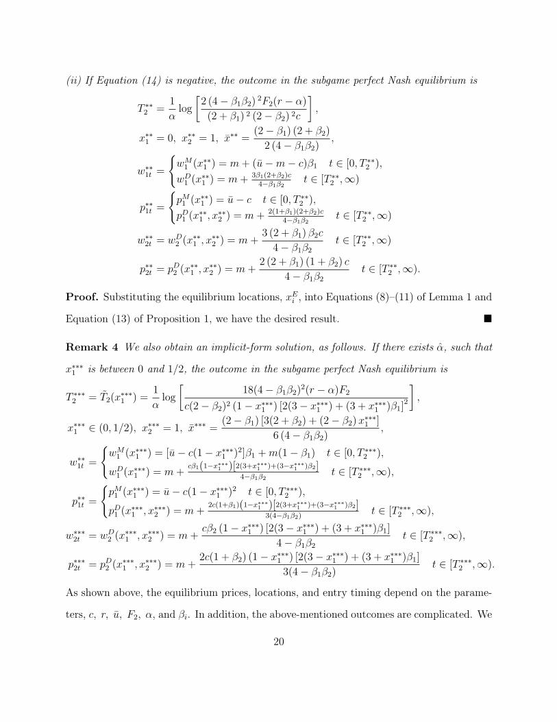
(ii) If Equation (14) is negative, the outcome in the subgame perfect Nash equilibrium is

T ∗∗2 =

1

αlog

[2 (4− β1β2)

2F2(r − α)

(2 + β1) 2 (2− β2) 2c

],

x∗∗1 = 0, x∗∗

2 = 1, x∗∗ =(2− β1) (2 + β2)

2 (4− β1β2),

w∗∗1t =

wM

1 (x∗∗1 ) = m+ (u−m− c)β1 t ∈ [0, T ∗∗

2 ),

wD1 (x

∗∗1 ) = m+ 3β1(2+β2)c

4−β1β2t ∈ [T ∗∗

2 ,∞)

p∗∗1t =

pM1 (x∗∗

1 ) = u− c t ∈ [0, T ∗∗2 ),

pD1 (x∗∗1 , x∗∗

2 ) = m+ 2(1+β1)(2+β2)c4−β1β2

t ∈ [T ∗∗2 ,∞)

w∗∗2t = wD

2 (x∗∗1 , x∗∗

2 ) = m+3 (2 + β1) β2c

4− β1β2

t ∈ [T ∗∗2 ,∞)

p∗∗2t = pD2 (x∗∗1 , x∗∗

2 ) = m+2 (2 + β1) (1 + β2) c

4− β1β2

t ∈ [T ∗∗2 ,∞).

Proof. Substituting the equilibrium locations, xEi , into Equations (8)–(11) of Lemma 1 and

Equation (13) of Proposition 1, we have the desired result.

Remark 4 We also obtain an implicit-form solution, as follows. If there exists α, such that

x∗∗∗1 is between 0 and 1/2, the outcome in the subgame perfect Nash equilibrium is

T ∗∗∗2 = T2(x

∗∗∗1 ) =

1

αlog

[18(4− β1β2)

2(r − α)F2

c(2− β2)2 (1− x∗∗∗1 ) [2(3− x∗∗∗

1 ) + (3 + x∗∗∗1 )β1]

2

],

x∗∗∗1 ∈ (0, 1/2), x∗∗∗

2 = 1, x∗∗∗ =(2− β1) [3(2 + β2) + (2− β2)x

∗∗∗1 ]

6 (4− β1β2),

w∗∗1t =

wM

1 (x∗∗∗1 ) = [u− c(1− x∗∗∗

1 )2]β1 +m(1− β1) t ∈ [0, T ∗∗∗2 ),

wD1 (x

∗∗∗1 ) = m+

cβ1(1−x∗∗∗1 )[2(3+x∗∗∗

1 )+(3−x∗∗∗1 )β2]

4−β1β2t ∈ [T ∗∗∗

2 ,∞),

p∗∗1t =

pM1 (x∗∗∗

1 ) = u− c(1− x∗∗∗1 )2 t ∈ [0, T ∗∗∗

2 ),

pD1 (x∗∗∗1 , x∗∗∗

2 ) = m+2c(1+β1)(1−x∗∗∗

1 )[2(3+x∗∗∗1 )+(3−x∗∗∗

1 )β2]3(4−β1β2)

t ∈ [T ∗∗∗2 ,∞),

w∗∗∗2t = wD

2 (x∗∗∗1 , x∗∗∗

2 ) = m+cβ2 (1− x∗∗∗

1 ) [2(3− x∗∗∗1 ) + (3 + x∗∗∗

1 )β1]

4− β1β2

t ∈ [T ∗∗∗2 ,∞),

p∗∗∗2t = pD2 (x∗∗∗1 , x∗∗∗

2 ) = m+2c(1 + β2) (1− x∗∗∗

1 ) [2(3− x∗∗∗1 ) + (3 + x∗∗∗

1 )β1]

3(4− β1β2)t ∈ [T ∗∗∗

2 ,∞).

As shown above, the equilibrium prices, locations, and entry timing depend on the parame-

ters, c, r, u, F2, α, and βi. In addition, the above-mentioned outcomes are complicated. We

20

confirm how these outcomes change using a numerical analysis, shown in Table 4 in Section

4.

4 Numerical analysis

To investigate the optimal location of group 1 and the total discounted values of the firms,

we conduct numerical analyses in Sections 4.1 and 4.2. First, Section 4.1 investigates the

effects of the parameters u (each consumer’s gross surplus for the product), c (consumer’s

transport cost), α (the growth rate of the market size), r (the interest rate), and F2 (group

2’s entry cost) on group 1’s equilibrium location, denoted as xE1 ∈ x∗

1, x∗∗1 , x∗∗∗

1 . Then,

Section 4.2 investigates the effects of the bargaining power, βi, on xE1 . In particular, we

show that a non-monotonic relationship exists between β1 and xE1 .

4.1 The Effects of c, m, r, u, F2, and α on xE1

Before discussing the effects of the suppliers’ bargaining power βi, which are the most im-

portant factors in our model, we summarize the effects of c, m, r, u, F2, and α on xE1 by

considering Equation (14). The fundamental properties behind the effects of c, m, r, u, F2,

and α on x1 are the same as those demonstrated by Ebina et al. (2015).

With regard to u, r, and F2, if one of these parameters increases, group 1 weighs the

importance of the monopoly phase more highly, yielding higher xE1 . Intuitively, an increase

in u increases only the profit of group 1 in the monopoly phase. Both an increase in r and

in F2 delay entry by group 2 by increasing its real entry cost, implying a longer duration of

the monopoly phase.

With regard to c and α, if one of these parameters increases, group 1 weighs the duopoly

phase more highly, because such an increase makes entry by group 2 easier as a result of the

greater product differentiation between D1 and D2 and the faster market growth.

21

Changing these parameters affects xE1 . The fundamental direction of these effects is

summarized in Table 1

c r u F2 α xE1

xE2 1 1 1 1 1

Table 1: Locations of firms 1 and 2, when c, r, u, F2, or α increases. xE1 means the

location of firm 1 approaches 0.5 (the center), whereas xE1 means the location of firm 1

approaches 0 (the edge).

4.2 The effects of β1 and β2 on xE1

We illustrate the relationship between the bargaining powers, β1 and β2, and the equilibrium

location of group 1, xE1 , in the case where u = 25 (see Table 2).

β1\β2 0.05 0.1 0.15 0.2 0.25 0.3 0.35 · · · 1

0.1 0.5 0.5 0.259 0.140 0.035 0 0 · · · 00.2 0.5 0.5 0.283 0.149 0.039 0 0 · · · 00.3 0.5 0.5 0.336 0.167 0.048 0 0 · · · 00.4 0.5 0.5 0.5 0.197 0.063 0 0 · · · 00.5 0.5 0.5 0.5 0.251 0.088 0 0 · · · 00.6 0.5 0.5 0.5 0.5 0.128 0 0 · · · 00.7 0.5 0.5 0.5 0.5 0.198 0.019 0 · · · 00.8 0.5 0.5 0.5 0.5 0.5 0.074 0 · · · 00.9 0.5 0.5 0.5 0.5 0.5 0.5 0 · · · 0

Table 2: The equilibrium location xE1 for F2 = 1000, c = 1, m = 1, r = 0.1, u = 25,

α = 0.0988, when β1 ∈ (0, 21/23) and β2 ∈ [0, 1].

First, we consider how β2 affects xE1 . Table 2 shows that as the bargaining power of

U2, β2, increases, the optimal location of group 1, xE1 , monotonically decreases for given

β1. The reason has already mentioned in Remark 3; that is, accelerating the downstream

competition through an increase in x1 substantially decreases w2t, which is higher owing to

22

larger β2. Thus, x1 becomes lower when β2 is larger. The inverse relation between β2 and

xE1 holds on most of the parameter space (c,m, r, u, F2, α).

Second, we consider how β1 affects xE1 . As in the decomposition in (14), the location

decision of group 1 depends on three effects: (I) the entry-delay effect, (II) the monopoly-gain

effect; and (III) the duopoly-gain effect. From (I), the center (xE1 = 1/2) is the best option

and the edge (xE1 = 0) is the worst option. This is because the ex post stronger competition,

achieved by a central location of D1, reduces the profitability of group 2, inducing group

2 to delay its entry. This effect is multiplied by the difference between the profits under

the monopoly and the duopoly, ΠM1 (x1)−ΠD

1 (x1). The higher β1 is, the stronger the factor

is, because an increase in β1 increases ΠM1 (x1) directly, owing to the stronger bargaining

power, and diminishes ΠD1 (x1) owing to the weaker competitiveness of group 1.15 From (II),

the center is the best option and the edge is the worst option, because the monopoly price

is constrained by the transportation cost of the furthest consumer from D1, and x1 = 1/2

minimizes this cost. As in (I), the higher β1 is, the stronger the factor is.16 From (III),

the edge is the best option and the center is the worst option, as in the standard spatial

competition. The higher β1 is, the weaker the competitiveness of group 1 is, inducing group

1 to locate closer to the edge.17 If the effects of (I) and (II) dominate that of (III), an increase

in β1 induces group 1 to locate closer to the center, as in Table 2.

Note that the monotonic relation between β1 and xE1 does not always hold. To understand

15 Note that, from Lemma 4, the higher β1 is, the lower dT2(x1)/dx1 is, because a higher β1 leads to a

higher w1, which eases the barrier to entry for group 2. This effect is not that strong, because an increase

in β1 indirectly influences group 2’s timing decision through the strategic interaction in the downstream

market.16 Note that an increase in β1 diminishes the first fraction of the second term in (14) through a decrease

in T2(x1), which diminishes the second term. In the subsequent numerical example, this decrease is offset

by the enhancement mentioned in the main text.17 Note that an increase in β1 increases the first fraction of the third term in (14) through a decrease in

T2(x1), which increases the absolute value of the third term.

23

the complexity of the relation between β1 and xE1 , we investigate the relative sizes of the

three terms in Equation (14). Using the parameters and group 1’s location xE1 , we derive

concrete values of Equation (14) for β1 ∈ (0, 0.9]. The common parameter values are c = 1,

m = 1, r = 0.1, u = 25, F2 = 1000, α = 0.0982, and β2 = 0.5. The result is summarized in

Table 3. The “Sum” column in Table 3 indicates how U1 decides its location. If the value in

the column is negative, then U1 locates at 0. However, if the value is positive, then U1 locates

at 1/2. If the value is 0, an interior location between 0 and 1/2 arises. As discussed earlier,

each term in Table 3 monotonically changes with an increase in β1, except for the change

between β1 = 0.45 and β1 = 0.5 in the second term (from 12.1 to 10.9). The exception comes

from the substantial change of xE1 , from 0.051 to 0.5. This table shows an example in which

the relation between β1 and xE1 is non-monotonic.

Third, we consider how α and β2 influence the relationship between β1 and xE1 . Suppose

that c = 1, m = 1, r = 0.1, u = 25, and F2 = 1000. The three figures in Figure 1 depict how

α influences the relation between β1 and xE1 under β2 = 0.25, β2 = 0.5, and β2 = 0.75. The

top inequality in each figure (e.g., α ≤ 0.0986 in Figure 1(a)) and the bottom inequality in

each figure (e.g., α ≥ 0.0991 in Figure 1(a)) show that xE1 = 0.5 and xE

1 = 0 become the

respective equilibrium locations under these ranges of α.

Figure 1(a) indicates that as α increases (decreases, respectively), xE1 becomes closer to

the edge (center, respectively). This result, which is explained in the previous section, is

the same as shown in Ebina et al. (2015). As α increases, the duopoly phase becomes

longer, inducing group 1 to locate closer to the edge. On the other hand, as α decreases,

the monopoly phase becomes longer, inducing group 1 to locate closer to the center. When

β2 = 0.25 in Figure 1(a), xE1 is increasing with β1. In contrast, when β2 = 0.5 and β2 = 0.75

in Figures 1(b) and 1(c), respectively, xE1 is not always increasing with β1. Figures 1(b)

and 1(c) show an interesting property that the equilibrium location becomes U-shaped with

24

β1 xE1 (I) First term (II) Second term (III) Third term Sum

0.0001 0.5 0.0623 0.00289 −0.0611 0.004070.05 0.5 30.7 1.41 −30.2 1.880.1 0.090 37.4 3.43 −40.8 00.15 0.072 54.3 4.99 −59.3 00.2 0.059 70.4 6.45 −76.8 00.25 0.050 85.9 7.79 −93.7 00.3 0.044 101 9.02 −110 00.35 0.043 116 10.1 −126 00.4 0.044 131 11.2 −142 00.45 0.051 146 12.1 −158 00.5 0.5 277 10.9 −264 23.50.55 0.5 302 11.6 −285 28.30.6 0.5 326 12.3 −305 34.10.65 0.5 351 13.0 −323 41.00.7 0.5 375 13.5 −340 48.50.75 0.5 399 14.1 −355 57.30.8 0.5 422 14.5 −369 67.40.85 0.5 446 15.0 −382 78.80.9 0.5 469 15.3 −393 91.7

Table 3: Values of the three terms in Equation (14) when c = 1, m = 1, r = 0.1, u = 25,F2 = 1000, α = 0.0982, and β2 = 0.5.

respect to β1. In particular, with regard to Figure 1(b), xE1 is in the range (0, 1/2) if β1

is neither small nor large; otherwise, xE1 is 0 or 1/2. Because there is no clear-cut relation

between β1 and the three significant effects (I), (II), and (III), a non-monotonic relationship

between β1 and xE1 can emerge, as in Table 3.

From the three figures in Figure 1, we determine how β2 influences the curve of x1 for

each α. When β2 = 0.25, xE1 is (almost) monotonically increasing with β1; when β2 = 0.5,

xE1 forms a U-shape with respect to β1 and reaches the bottom around β1 ∈ [0.25, 0.3]; when

β2 = 0.75, xE1 suddenly changes from one corner solution to the other, and reaches the

bottom around β1 ∈ [0.45, 0.65].

It may seem that the discussion in this subsection implies that a manufacturer that needs

25

Figure 1: The relationship between β1 ∈ (0, 21/23) and xE1 , when (a) β2 = 0.25 (upper left),

(b) β2 = 0.5 (upper right), and (c) β2 = 0.75 (bottom).

a downstream agent to launch a new product faces a difficulty in determining its optimal

product position if it anticipates the subsequent entry of another supplier, and the market

growth rate α is close to the interest rate r (if these do not hold, the optimal location is the

center of the Hotelling line). However, we do not think that the non-monotonic relationship

between β1 and xE1 is a serious problem for U1. In other words, we do not think that the

significant jump of xE1 as a result of an increase in β1 makes U1 difficult to choose its optimal

location. In fact, under the parameter set in Figure 2, which is explained later, V1 has two

locally maximum points with respect to x1, and this multiplicity of locally optimal points

causes the substantial jump of xE1 from one of the two to the other. Thus, as shown in

Figure 2 later, V1 smoothly changes with β1, even when x1 jumps substantially from one of

26

the locally optimal points to another as a result of an increase in β1. Therefore, the complex

relation between β1 and xE1 is not that serious for U1, but would be serious for U2, as shown

in Figure 2, later.

4.3 The effect of β1 on T2(xE1 )

Table 4 shows a non-monotonic relationship between β1 and T2(xE1 ) through a monotonic

increase in xE1 . An increase in β1 has two contrasting effects. First, increasing β1 itself

decreases T2(x1) for a fixed x1, as shown in Corollary 1. Second, increasing β1 makes xE1

closer to the center, yielding an increase in T2(xE1 ) through stronger duopoly competition. We

explain the two contrasting effects here using Table 4. When β1 ∈ (0, 0.5], the former effect

dominates the latter effect; T2(xE1 ) decreases, because xE

1 moves toward the center slowly in

accordance with an increase in β1. In contrast, when β1 ∈ [0.5, 0.7], the movement of xE1

accelerates, so that the latter effect dominates the former effect; T2(xE1 ) increases. Moreover,

when β1 ∈ [0.7, 21/23), this trend suddenly changes, because xE1 reaches 1/2 (the center),

and the latter effects vanish. This is why T2(xE1 ) decreases again when β1 ∈ [0.7, 21/23).

β2 β1 xE1 xE

2 TE2 pM1 wM

1 pD1 wD1 pD2 wD

2

0.1 0.001 0.120 1 10.1 24.2 1.02 1.96 1.00 1.93 1.130.1 0.1 0.126 1 9.14 24.2 3.32 2.05 1.14 1.97 1.130.1 0.2 0.136 1 8.26 24.3 5.65 2.14 1.28 2.01 1.140.1 0.3 0.153 1 7.52 24.3 7.98 2.22 1.42 2.04 1.140.1 0.4 0.178 1 6.94 24.3 10.3 2.29 1.55 2.05 1.140.1 0.5 0.215 1 6.60 24.4 12.7 2.33 1.67 2.05 1.140.1 0.6 0.276 1 6.72 24.5 15.1 2.34 1.75 2.00 1.140.1 0.7 0.5 1 10.3 24.8 17.6 2.05 1.65 1.70 1.090.1 0.8 0.5 1 9.33 24.8 20 2.11 1.74 1.73 1.100.1 0.9 0.5 1 8.39 24.8 22.4 2.17 1.83 1.76 1.100.1 21/23 0.5 1 8.27 24.8 22.7 2.18 1.85 1.77 1.10

Table 4: The outcome of the subgame perfect Nash equilibrium depending on β1 and β2

when c = 1, m = 1, r = 0.1, u = 25, F2 = 1000, and α = 0.099.

27

4.4 Effects of bargaining power on the total values

In this subsection, we investigate how the bargaining power of group 1, β1, affects the

total values of the firms (U1, D1, U2, and D2), V1, v1, V2, and v2. These relationships are

summarized in Figure 2. Suppose that c = 1, m = 1, r = 0.1, u = 25, F1 = 0, and F2 = 1000.

Figure 2: The relationship between β1 ∈ (0, 21/23) and the total values V1 and v1 in equi-librium when (a) α = 0.0982 (upper left), and (b) α = 0.09825 (upper right); and therelationship between β1 ∈ (0, 21/23) and V2 in equilibrium when (c) α = 0.0982 (lowerright), and (d) when α = 0.09825 (lower left).

Figures (a) and (b) in Figure 2 depict the relationship between β1 and V1 and that

between β1 and v1 under α = 0.0982 and α = 0.09825, respectively. These include the case

of β2 = 0.5, which is the same as that shown in Figure 1(b). We can easily confirm that the

total value of U1 strictly increases with β1, although that of D1 strictly decreases with β1.

28

Note that v1 drops at some β1 when xE1 changes substantially with an increase in β1. For

example, in Figure 2(a), v1|β2=0.5 drops at β1 = 0.1. Furthermore, Figures 2(a) and (b) show

a non-monotonic relationship between v1 and β2, although the relationship between V1 and

β2 is monotonic. With regard to Figure 2(a), v1|β2=0.4 ≥ v1|β2=0.5 holds for β1 ∈ [0.1, 0.2],

though v1|β2=0.4 < v1|β2=0.5 holds for β1 ∈ (0, 0.1) and for β1 ∈ (0.2, 21/23). With regard to

Figure 2(b), we see a similar relationship, where v1|β2=0.4 ≥ v1|β2=0.5 holds for β1 ∈ (0, 0.2],

though v1|β2=0.4 < v1|β2=0.5 holds for β1 ∈ (0.2, 21/23).

As mentioned in the last paragraph in Section 4.2, the non-monotonic relationship be-

tween xE1 and β1 has a significant impact on U2. To understand the relation between the

non-monotonic relationship and V2, we focus on the case of α = 0.0982 in Figure 1(b) and

V2|β2=0.5 in Figure 2(c). When α = 0.0982 in Figure 1(b), xE1 drops substantially from 1/2

to about 0.1 when β1 moves from 0.05 to 0.1; xE1 moves around 0.075 when β1 is in the range

[0.1, 0.45]; and xE1 jumps up substantially from about 0.05 to 1/2 when β1 moves from 0.45 to

0.5. Related to the substantial drop and the substantial jump around β1 = 0.1 and β1 = 0.5,

respectively, V2|β2=0.5 in Figure 2(c) jumps significantly at β1 = 0.1, and drops significantly

at β1 = 0.5. Furthermore, for other values of β2, in Figures 2(c) and (d), we observe that

V2 drops or jumps substantially, which is related to the non-monotonic relationship between

xE1 and β1. Therefore, we conclude that the complex relation between xE

1 and β1 has a

significant impact on U2.

5 Discussion

We discuss how changing the assumption of U2’s strong position over D2 in the entry timing

affects our results in Section 5.1. Then, we discuss whether changing from asymmetric to

symmetric bargaining power affects our result in Section 5.2.

29

5.1 Difference between this model and the model of Ebina et al.(2015)

In this subsection, we examine whether changing the assumption of U2’s strong position over

D2 in the entry timing to reflect that in Ebina et al. (2015) affects our main results.

Before proceeding with the analysis, we briefly check the entry decisions of group 2 (firm

2) in this study and those in Ebina et al. (2015). The optimal entry timing of firm 2

(follower) under the setting of Ebina et al. (2015) is

T2(x1) =1

αlog

[rF2

πD2 (x1)

]=

1

αlog

[18rF2

c(1− x1)(3− x1)2

], (18)

where πD2 (x1) = c(1 − x1)(3 − x1)

2/18 denotes the duopoly profit of firm 2, whereas the

optimal timing of group 2 in our setting is given in Equation (13). There are two differences

between the two studies. The first stems from the difference in the duopoly profits, which

is based on whether vertical relations exist. This difference in the duopoly profits changes

the difference from π2(x1) to π2(x1). The second stems from the difference in the criteria

for market entry. In Ebina et al. (2015), the follower has the freedom to choose when it

enters the market. In contrast, U2 maximizes its profit by choosing T2, which satisfies the

zero-profit condition for D2. This difference makes group 2 enter sooner, with the timing

changing from r to r − α, which corresponds to the numerator inside the logarithm in (13).

Thus, changing the second assumption on the criteria for market entry made in this study

to that made in Ebina et al. (2015), we have

∂v2∂T2

= 0

⇒T2(x1) =1

αlog

[rF2

πD2 (x1)

]=

1

αlog

[18(4− β1β2)

2rF2

c(2− β2)2 (1− x∗∗∗1 ) [2(3− x∗∗∗

1 ) + (3 + x∗∗∗1 )β1]

2

].

Next, we conduct a numerical analysis using the same parameter values in Section 4.

Suppose that r = 0.1, F2 = 1000, c = 1, and m = 25, which are the same as in Figures 1(b)

30

and (c). When β2 = 0.5 and 0.75, the equilibrium location pattern of group 1 is as shown in

Figures 3(a) and (b), respectively.

Figure 3: The relationship between the equilibrium location of group 1 and β1 ∈ (0, 21/23)under the setting of Ebina et al. (2015) when (a) β2 = 0.5 (left) and (b) β2 = 0.75 (right).

Comparing Figures 1(b) and 3(a) (Figures 1(c) and 3(b), respectively), a slight increase

in β2 has a similar impact on xE1 in both this study and that of Ebina et al. (2015).18 This is

because the sign of the first-order derivatives of T2 and T2 with respect to the parameters are

the same. Therefore, we verify that the U-shaped nature of xE1 on β2, which is an interesting

finding of this study, depends on the vertical relationship, but does not depend on the market

entry criteria for the follower.

5.2 Symmetric bargaining power

Many studies assume symmetric bargaining power, in the sense that the bargaining pow-

ers of all firms are equal (β1 = β2(≡ β)), and investigate firms’ behavior under vertical

relationships.19 In this subsection, we briefly discuss how employing the assumption of sym-

18 We also conduct a numerical analysis under the setting of Ebina et al. (2015) when β2 = 0.9, and obtain

a figure that shows a sudden change of xE1 from one corner solution to the other corner solution, similarly

to Figure 1(c). We omit the figure owing to space limitations.19 See, for instance, the non-spatial oligopoly model in Horn and Wolinsky (1988).

31

metric bargaining power affects our main results.

Figure 4(a) depicts the relationship between β and xE1 when α changes. Suppose that

c = 1, m = 1, r = 0.1, u = 25, and F2 = 1000. This setting is the same as that in

Figure 1, and the result is summarized in Table 3. In contrast to the asymmetric case shown

in Figure 1, where xE1 can be increasing or U-shaped, we confirm that xE

1 is decreasing

in β. This relationship is strong, because the rival’s wholesale price reduction owing to the

narrower distance betweenD1 andD2 is strong. Thus, although many studies consider a Nash

bargaining problem under symmetric bargaining in a discrete time model, it is important to

consider asymmetric bargaining power when examining a vertical relationship through Nash

bargaining by employing a continuous-time model.

Figure 4: The relationship between (a) the equilibrium location of group 1 and symmetricbargaining power β (left) and (b) xE

1 and the bargaining power of group 2 β2 when β1 = 0.5(right).

Finally, we briefly discuss the relationship between xE1 and β2. Figure 4(b) depicts the

relationship between β2 ∈ [0, 1) and xE1 when β1 = 0.5. The settings of the other parameters

are the same as in the symmetric case. The fundamental shapes of the graphs, which are

downward sloping, are similar to the symmetric case, and for the same reason. Thus, we

focus only on the relationship between β1 and xE1 , and on the values of the firms in the

32

previous section.

6 Conclusion

This study investigates a dynamic Hotelling duopoly model with endogenous entry timing

and location choices under vertical contracting. We focus on how upstream suppliers’ bar-

gaining power over their downstream buyers (β1 and β2) influence the locations (x1 and x2)

and the entry timing of the follower pair (T2). A larger β1 usually induces a larger x1 and,

thus, a larger T2. This implies that the stronger bargaining power of the supplier can also

benefit the downstream buyer; that is, it might be better for a downstream buyer to weaken

its bargaining position over its trading supplier. In addition, under some sets of exogenous

parameters, there is a non-monotonic relation between β1 and x1. More specifically, the

equilibrium location of the leader pair can jump substantially with an increase in β1, which

significantly delays T2 and diminishes the profitability of the follower pair. Moreover, a

larger β2 induces a smaller x1, which facilitates the earlier entry of the follower pair. This

implies that when an upstream manufacturer tries to enter a newly growing market with

its downstream representative, it needs to maintain its strong bargaining power over the

representative.

This study shows that the bargaining power of an upstream manufacturer/franchiser

over a downstream representative/franchisee affects the entry timings and location points.

As mentioned in the introduction, several studies emphasize that large national retailers tend

to have strong bargaining power over their upstream firms (Geylani et al., 2007; Inderst and

Shaffer, 2007, 2009). Our results indicate that location points and entry timings are strongly

affected by such bargaining power. Our theoretical results suggest that as the bargaining

powers strengthen, the location of group 1 will move closer to an interior, or center (not the

edge), and that group 2 will wait longer before entering a new market.

33

We assume that the leader immediately enters the market (i.e., T1 = 0). As in Ebina et

al. (2017), considering the endogenous entry timing of the leader pair is a topic for future

research, although it substantially complicates the analysis. In addition, future research can

explore a more sophisticated contract term, such as a two-part tariff contract, as in Alpranti

et al. (2015).

7 Appendix

We explain the condition in which the market is fully covered by D1 in the monopoly case.

The profit of D1 is given as

πM1t (x1) =

(p1t − w1t) if p1t ≤ u− c(1− x1)2,

(p1t − w1t)

[√u− p1t

c+ x1

]if u− c(1− x1)

2 < p1t ≤ u− cx21,

2(p1t − w1t)

√u− p1t

cif u− cx2

1 < p1t ≤ u.

The first-order condition is given as

∂πM1t (x1)

∂p1t=

1 if p1t ≤ u− c(1− x1)2,

x1 +2u− 3p1t + w1t

2√

c(u− p1t)if u− c(1− x1)

2 < p1t ≤ u− cx21,

2u− 3p1t + w1t

2√c(u− p1t)

if u− cx21 < p1t ≤ u.

We show the condition that the optimal price of D1 at each t ∈ [0, T2) is p1t = u− c(1−

x1)2, which is the maximum price among those that lead to full coverage of the market.

When u− c(1− x1)2 < p1t ≤ u− cx2

1, the second-order condition is

∂2πM1t (x1)

∂p21t=

−4u+ 3p1t + w1t

4√c(u− p1t)

√u− p1t

(< 0).

Under this range of p1t, πM1t (x1) monotonically decreases with p1t if the following inequality

holds:

∂πM1t (x1)

∂p1t

∣∣∣∣↓p1=u−c(1−x1)2

= 1− u− c(1− x1)2 − w1t

2c(1− x1)< 0;

34

that is,

w1t < u− c(1− x1)(3− x1). (19)

If w1t does not satisfy the inequality, this w1t does not maximize the joint profit in group 1

because the market demand is not fully covered.

When the firms in group 1 anticipate that D1 sets p1t(x1) = u− c(1− x1)2 in the pricing

stage, the bargaining outcome in the negotiation stage is

β1 : 1−β1 = (w1t−m) : u−c(1−x1)2−w1t → w1t(x1) = β1(u−c(1−x1)

2)+(1−β1)m. (20)

If this w1t(x1) satisfies the inequality in (19), D1 actually sets p1t(x1) = u− c(1−x1)2, given

w1t(x1) = β1(u− c(1− x1)2) + (1− β1)m. Substituting w1t in (20) into (19), we obtain

c(1− x1)(3− x1 − β1(1− x1)) < (1− β1)(u−m).

This becomes the most stringent condition when the left-hand side is maximized. For x1 ∈

[0, 1/2], it is maximized at x1 = 0, and then the condition becomes

c(3− β1) < (1− β1)(u−m) → β1 <u−m− 3c

u−m− c.

References

Alipranti, M., C. Milliou, E. Petrakis. 2015. On vertical relations and the timing oftechnology adoption. Journal of Economic Behavior & Organization 120, 117–129.

Brekke, K.R., O.R. Straume. 2004. Bilateral monopolies and location choice. RegionalScience and Urban Economics 34(3), 275–288.

Bronnenberg, B.J., V. Mahajan. 2001. Unobserved retailer behavior in multimarket data:Joint spatial dependence in market shares and promotion variables. Marketing Science20(3), 284–299.

Chen, Z. 2003. Dominant retailers and the countervailing-power hypothesis. RAND journalof Economics 34(4), 612–625.

35

Cleeren, K., F. Verboven, M.G. Dekimpe, K. Gielens. 2010. Intra- and inter-format com-petition among discounters and supermarkets. Marketing Science 29(3), 456–473.

d’Aspremont, C., J.-J. Gabszewicz, J.-F. Thisse. 1979. On Hotelling’s stability in compe-tition. Econometrica 47(5), 1145–1150.

Desai, P.S. 2001. Quality segmentation in spatial markets: When does cannibalizationaffect product line design? Marketing Science 20(3), 265–283.

Dobson, P.W., M. Waterson. 1997. Countervailing power and consumer prices. EconomicJournal 107(441), 418–430.

Draganska, M., M. Mazzeo, K. Seim. 2009. Beyond plain vanilla: Modeling joint productassortment and pricing decisions. Quantitative Marketing and Economics 7(2), 105–146.

Dukes, A.J., E. Gal-Or, K. Srinivasan. 2006. Channel bargaining with retailer asymmetry.Journal of Marketing Research 63(1), 84–97.

Ebina, T., N. Matsushima, K. Nishide. 2017. Demand uncertainty, product differentia-tion, and entry timing under spatial competition. ISER Discussion Paper No.1007.Available at https://ideas.repec.org/p/dpr/wpaper/1007.html

Ebina, T., N. Matsushima, D. Shimizu. 2015. Product differentiation and entry timing in acontinuous time spatial competition model. European Journal of Operational Research247(3), 904–913.

Erkal, N. 2007. Buyer–supplier interaction, asset specificity, and product choice. Interna-tional Journal of Industrial Organization 25(5), 988–1010.

Geylani, T., A.J. Dukes, K. Srinivasan. 2007. Strategic manufacturer response to a domi-nant retailer. Marketing Science 26(2), 164–178.

Gotz, G. 2005. Endogenous sequential entry in a spatial model revisited. InternationalJournal of Industrial Organization 23(3-4), 249–261.

Hauser, J.R. 1988. Competitive price and positioning strategies. Marketing Science 7(1),76–91.

Horn, H., A. Wolinsky. 1988. Bilateral monopolies and incentives for merger. RANDJournal of Economics 19(3), 408–419.

Hwang, M., B.J. Bronnenberg, R. Thomadsen. 2010. An empirical analysis of assortmentsimilarities across U.S. supermarkets. Marketing Science 29(5), 858–879.

Inderst, R., G. Shaffer. 2007. Retail mergers, buyer power and product variety. EconomicJournal 117(516), 45–67.

36

Inderst, R., G. Shaffer. 2009. Market power, price discrimination, and allocative efficiencyin intermediate-goods markets. RAND Journal of Economics 40(4), 658–672.

Kim, H., K. Serfes. 2006. A location model with preference for variety. Journal of IndustrialEconomics 54(4), 569–595.

Kuksov, D. 2004. Buyer search costs and endogenous product design. Marketing Science23(4), 490–499.

Lambertini, L. 2002. Equilibrium locations in a spatial model with sequential entry in realtime. Regional Science and Urban Economics 32(1), 47–58.

Liu, Y., R.K. Tyagi 2011. The benefits of competitive upward channel decentralization.Management Science 57(4), 741–751.

Loertscher, S., G. Muehlheusser. 2011. Sequential location games. RAND Journal ofEconomics 42(4), 639–663.

Matsumura, T., N. Matsushima. 2009. Cost differentials and mixed strategy equilibria ina Hotelling model. Annals of Regional Science 43(1), 215–234.

Matsushima, N. 2004. Technology of upstream firms and equilibrium product differentia-tion. International Journal of Industrial Organization 22(8–9), 1091–1114.

Matsushima, N. 2009. Vertical mergers and product differentiation. Journal of IndustrialEconomics 57(4), 812–834.

Matsushima, N., A. Miyaoka. 2015. The effects of resale-below-cost laws in the presence ofa strategic manufacturer. Quantitative Marketing and Economics 13(1), 59–91.

Matsushima, N., C. Pan. 2016. Strategic perils of outsourcing: Sourcing strategy andproduct positioning. ISER Discussion Paper No. 983.

Available at https://ideas.repec.org/p/dpr/wpaper/0983.html

Moorthy, K.S. 1988. Product and price competition in a duopoly. Marketing Science 7(2),141–168.

Muthoo, A. 1999. Bargaining Theory with Applications. Cambridge University Press,Cambridge.

Orhun, A.Y. 2013. Spatial differentiation in the supermarket industry: The role of commoninformation. Quantitative Marketing and Economics 11(1), 3–37.

Peres, R., E. Muller., V. Mahajan. 2010. Innovation diffusion and new product growthmodels: A critical review and research directions. International Journal of Researchin Marketing 27(2), 91–106.

37

Raju, J., Z.J. Zhang. 2005. Channel coordination in the presence of a dominant retailer.Marketing Science 24(2), 254–262.

Raynaud, E., L. Saubee, E. Valceschini. 2009. Aligning branding strategies and governanceof vertical transactions in agri-food chains. Industrial and Corporate Change 18(5),835–868.

Reinartz, W., B. Dellaert, M. Krafft, V. Kumar, R. Varadarajan. 2011. Retailing innova-tions in a globalizing retail market environment. Journal of Retailing 87(S1), S53–S66.

Sajeesh, S. 2016. Influence of market-level and inter-firm differences in costs on productpositioning and pricing. Applied Economics Letters 23(12), 888–896.

Sajeesh, S., J. Raju. 2010. Positioning and pricing in a variety seeking market. ManagementScience, 56(6), 949–961.

Tabuchi, T., J.-F. Thisse. 1995. Asymmetric equilibria in spatial competition. Interna-tional Journal of Industrial Organization 13(2), 213–227.

Thomadsen, R. 2007. Product positioning and competition: The role of location in the fastfood industry. Marketing Science 26(6), 792–804.

Wernerfelt, B. 1986. Product line rivalry: Note. American Economic Review 76(4), 842–844.

Zhu, T., V. Singh. 2009. Spatial competition with endogenous location choices: An appli-cation to discount retailing. Quantitative Marketing and Economics 7(1), 1–35.

38