Product differentiation with variants, and welfare effects

of automobile engine options

Øyvind Thomassen∗

Katholieke Universiteit Leuven

December 4, 2010

Abstract

I develop a demand framework for markets where products (mod-els) have variants that differ only with respect to quantifiable productcharacteristics. There is an unobserved product characteristic anda consumer-specific logit term for models, but both are fixed acrossvariants. The literature’s assumption of orthogonality between unob-served and observed product characteristics is not needed. A counter-factual where car models are restricted to have just one engine optionshows that engine options increase profits in spite of tougher compe-tition. Consumer surplus and tax revenue from an engine-size-relatedtax also increase.

∗E-mail: oyvind.thomassen@econ.kuleuven.be. This is a revised version of chapter 1 ofmy 2009 Oxford DPhil thesis. A previous version was called Automobile engine variantsand price discrimination. Thanks to my thesis supervisor Howard Smith, examiners IanCrawford and Philipp Schmidt-Dengler, and Frank Verboven, Johannes Van Biesebroeckand Laura Grigolon for comments.

1

1 Introduction

It is a common practice for firms to offer variants of a given product which

differ only with respect to one or a few characteristics. Some examples are

the 16 and 32GB storage versions of the iPhone 4, different fat-levels of a

milk brand, economy and business class seats on a British Airways flight

from London to Paris, an internet service provider’s bandwidth packages,

a Volkswagen Golf with a 79 or 158hp engine1, and four- or six-core AMD

Phenom II processors.2

I define two goods as variants of the same product if they differ only with

respect to product characteristics that are quantifiable and generic. By quan-

tifiable I mean that there exists a generally accepted method for determining

how much of the characteristic a product has. A feature is generic if it does

not describe something like “being product X”. Horsepower is quantifiable

and generic. Prestige is generic but not quantifiable. Toyota is quantifiable

(with a 0-1 variable), but not generic.

The purpose of this article is (1) to point out that markets where products

have variants do not fit into existing demand models, (2) to develop an

alternative demand model for markets with variants, and (3) to use the model

to analyse how engine options affect profits and welfare in the car market.

In the differentiated-products demand literature starting with Berry (1994)

and Berry, Levinsohn, and Pakes (1995) (BLP), the utility a consumer gets

from a product is a linear function of observable product characteristics. In

addition, a product-specific constant captures unobserved product charac-

teristics that affect consumers in the same way. Finally, utility includes a

random shock that is iid across products and consumers. The shock repre-

1The output of a given engine can be adjusted by software settings of the engine controlunit.

2The four-core processor is physically the same as the six-core version, except with twocores disabled.

2

sents likes and dislikes that are idiosyncratic in the sense that a consumer’s

taste shock for product A provides no information about his taste shock for

product B, or about another consumer’s taste shocks, either for product A

or B.

These assumptions are not appropriate for markets with variants. Variants

differ only by quantifiable generic characteristics, which in practice means

observable variables. The effect of observable product characteristics is fully

accounted for by directly including these characteristics in the utility func-

tion. Therefore, a difference in utility between two variants must be fully

explained by the terms involving the observable characteristics. Letting ei-

ther the taste shock or the unobserved product characteristic vary across

variants of a product is therefore not justified, and imposes product differen-

tiation that does not exist in reality. Accordingly, the model in this paper has

unobserved characteristics and idiosyncratic taste shocks at the model-level,

but not at the variant level.

I keep the substantive assumptions of the recent automobile demand liter-

ature3 that there are unobserved differences and idiosyncratic tastes for car

models.4 As in many markets, it is plausible that consumers have real id-

iosyncratic tastes for models. When this is the case, removing the iid shock

altogether, as in Bajari and Benkard (2005) and Berry and Pakes (2007),

would underestimate product differentiation.

The taste for products introduces a new dimension of product differentia-

tion for each product. Petrin (2002) discusses how this may overestimate

the benefits of introducing new goods, since some consumers will have a

very large idiosyncratic taste premium for every new product over existing

ones, no matter how similar it is to existing products. In this paper shocks

3BLP, Petrin (2002), Berry, Levinsohn, and Pakes (2004).4The literature abstracts away from the variant issue: each consumer chooses a car

model whose price and engine characteristics are chosen by the researcher from among themodel’s range of engine variants. This is likely to affect the estimated coefficients on priceand engine characteristics.

3

enter only at the model level. Therefore the number of dimensions of prod-

uct differentiation does not vary when the number of variants per model is

changed.

The demand model permits identification with weaker assumptions than in

the literature. Goldberg (1995) restricts the unobserved product character-

istic to be the same across car models of a given brand. Brand-level fixed

effects control for unobservable characteristics. BLP relax this assumption by

including model-specific dummies to control for unobservables at the model

level. But these dummies capture the mean effect of observed characteris-

tics as well as unobserved characteristics. To separate the two effects, BLP

need to assume orthogonality between unobserved and observed characteris-

tics and instruments for price (since price is correlated with the unobserved

characteristic). Any model that allows for alternative-specific unobservables

needs this orthogonality assumption.5 However, the assumption is problem-

atic because both types of product characteristics are choice variables of

manufacturers.6

I relax both the orthogonality assumption of BLP and Goldberg’s restriction

that unobservables are fixed across models of a brand. Since unobservables

do not vary across variants, I can control for unobservables with model-level

fixed effects. My error term is an individual-level prediction error explained

by sampling error, as is standard in micro-data discrete-choice models. Since

all unobservable product characteristics are captured by the fixed effects,

they are not in the error term. It follows that price is not endogenous, so

no instrumental variables are needed. Price and product characteristics vary

within models, so that their effects are separately identified.

In the car market, models, such as Volkswagen Golf, Toyota Camry, or BMW

5BLP micro (Berry, Levinsohn, and Pakes 2004) in principle need it too, but insteaduse calibration to find the unidentified parameters.

6E.g. Ackerberg, Benkard, Berry, and Pakes (2007) p. 4197 say: “There are plausi-ble reasons to believe that product characteristics themselves are correlated with ξ [theunobservable]”.

4

3-series, differ in the eye of the consumer with respect to design, prestige,

dealership/service access, advertising exposure and other features that are

usually both unobservable for researchers and partly uncorrelated across con-

sumers and products. In addition to models there is extensive product dif-

ferentiation through variants: options with respect to mechanical internals

(engine, transmission), body style and trim levels increase the total number

of products enormously. For instance a new Volkswagen Golf has 15 engine

variants and Peugeot 407 has 13. Focusing on engine variants, I ask whether

this differentiation is excessive from the point of view of car companies, and

to what extent it benefits consumers.

Dixit and Stiglitz (1977) discuss how two opposite effects may mean that ei-

ther too few or too many products are introduced: introducing a new product

has a positive externality on consumers, because the firm cannot capture the

entire consumer surplus, and a negative externality on other firms because

of business stealing. In a model with vertical and horizontal differentiation

similar to the empirical model in this paper, Gilbert and Matutes (1993)

show that firms may offer several qualities each when they would be better

off committing to offer only one, again because they do not take into account

the business stealing externality on other firms.

I look at a simple counterfactual where I restrict each car model to have only

one engine option.7 Comparing equilibrium prices and sales to those in the

actual market, I find that going from one engine per model to the number

in fact offered has the following results: (1) Welfare increases through (a)

a 4.4% increase in consumer surplus, (b) an 8.9% increase in engine-size-

related tax revenues and VAT, and (c) a 2.4% increase in profits. (2) Profits

go up because of increased total sales (i.e. new consumers recruited from

the outside good because of increased product variety), in spite of a small

reduction in average markups.

7I assume firms would choose to keep the variant currently accounting for the highestprofits, and that there are no fixed cost savings in restricting the range of engine options.

5

The next section describes the utility model and derives the choice prob-

abilities. Section 3 explains the identification strategy and compares it to

the literature. Section 4 describes the data, and attempts to show that the

assumptions of the model are satisfied by the data. Section 5 describes the

estimator, section 6 the results. Section 7 gives the results from the counter-

factual experiment.

2 Model

2.1 Utility

I estimate the parameters of the conditional (on product choice) indirect

utility functions of potential car buyers. Products are grouped into mod-

els. Products within a model, called variants, differ only with respect to

observable characteristics. Products in different models differ with respect

to characteristics that are not observable to the researcher, but known by

market agents. Let J = {0, . . . , J} be the choice set, where j = 0 is the

outside good.8 Each product is described by a double (xj , m(j)) - a vector

of observable product characteristics and an index for the model to which

the product belongs. Let the vector x0j be the subvector of xj consisting of

the variant characteristics (all characteristics that vary across variants of a

model) and let x1m(j) be the remaining characteristics (model characteristics),

so xj = (x0j , x

1m(j)). Let pj be price, yi income, and zi a vector of observable

consumer characteristics. Conditional on choosing product j consumer i has

8Individuals or products are not followed across time. I.e. they have different subscriptsfor different years of data.

6

indirect utility:

uij = −(α + αi)pj + x0j (β

0 + β0i ) + x1

m(j)β1i + δm(j) + ǫim(j) (1)

ui0 = ξ0 + ǫi0 (2)

αi = α(zi, yi) (3)

βri = βr(zi, νi), r = 0, 1 (4)

ǫim(j) ∼ iid extreme value, (5)

where α and β are functions of consumer characteristics whose realisations

(zi) or distributions (yi, νi) are known.

The model mean effects, δ, can in theory be decomposed into the mean effect

of model characteristics and unobservable characteristics: δm = x1m(j)β

1 +

ξm. For most applications, the decomposition of δ is not required, nor is it

identified with the assumptions used in this paper. Unlike in the literature,

δ does not contain the mean effects of price and variant characteristics.

ξm+ ǫim captures the common and consumer-specific valuation of any aspect

of modelm that is not controlled for by the observable characteristics x. Since

variants of a model differ only with respect to observable characteristics x0

these terms have m-subscripts.

ǫ captures effects of unobservable characteristics which do not provide any

information about the unobservable effect of another product on the same

consumer, nor on the effect on a different consumer. An example is consumer

A who likes the look of VW Golf, but dislikes the Ford Focus; consumer B

who thinks the Golf is boring, and the Focus elegant; consumer C who likes

the look of the Golf, and loves the Focus.

7

2.2 Choice probabilities

Denote the ‘observable’ part of utility u− (δ + ǫ),

Vij = −(α + αi)pj + x0j (β

0 + β0i ) + x1

m(j)β1i .

Conditional on the realisations of the random variables (y, ν) the probability

that consumer i chooses model m is

Pr(m|i, y, ν) = Pr(maxj∈Jm

{Vij}+ δm + ǫim (6)

> maxj′∈Jm′

{Vij′}+ δm′ + ǫim′ , m′ 6= m|i, y, ν)

=exp(maxj∈Jm{Vij}+ δm)

1 +∑

m′∈M exp(maxj′∈Jm′{Vij′}+ δm′t), (7)

where Jm is the set of variants of model m, and M is the set of models in the

market. Conditional on (y, ν), the max{V }-terms are not random variables.

The second equality therefore follows in a standard way by integrating over

the distribution of the ǫ-term to obtain a logit choice probability.

Still conditional on (y, ν), consumer i’s probability of choosing j is equal to

Pr(m|i, y, ν) if j maximises {Vij} over Jm, and zero otherwise. Letting the

indicator function 1[j|m, i, y, ν] be one in the first case and zero in the second

case, we can write the choice probability of product j

Pr(j|i, y, ν) = 1[j|m, i, y, ν]exp(maxj∈Jm{Vij}+ δm)

1 +∑

m′∈M exp(maxj′∈Jm{Vij′}+ δm′). (8)

Integrating over the distributions of y and ν, we now get consumer i’s un-

conditional choice probability for product j

Pr(j|i) =

∫ ∫

Pr(j|i, y, ν)f(y|i)f(ν)dydν, (9)

where f(ν) is the joint density of ν, and f(y|i) is the density of the em-

8

pirical income distribution in the population for consumers with observed

characteristics zi in the time period t(i) in which i enters the data.

3 Identification

The model is estimated by assuming orthogonality between the individual-

level prediction error (difference between observed choices and choice prob-

abilities) and explanatory variables. This error term is distinct from the

literature’s unobserved product characteristic. I control for unobserved prod-

uct characteristics using fixed effects for car models in the utility function.

Unobserved product characteristics therefore do not enter the error term.

The error term is pure sampling error. Price and product characteristics are

therefore exogenous. I do not need orthogonality between unobserved and

observed product characteristics to identify the price parameter, since it is

identified by within-model variation separately from model fixed effects.

3.1 Unobserved product characteristics and identifying assumptions

In discrete-choice demand models consumers choose among alternatives by

maximising a utility function that depends on observed product character-

istics. But typically consumers also care about product characteristics that

are not observed by the researcher. Berry (1994) and BLP solve this problem

by introducing product-specific constants in utility.

The product-specific constants ensure that utility includes the effect of unob-

servables. But the product-specific constants also capture the mean (across

consumers) effect of price and observed characteristics. In order to separate

the two effects, the literature assumes that unobserved and observed prod-

uct characteristics are orthogonal.9 That is, the observed characteristics of a

9When observations are at the level of products, like in BLP, the orthogonality assump-

9

product provides no information that affects the expected value of the unob-

served characteristic of that product. Since both unobserved and observed

characteristics are choice variables of firms, this assumption is problematic.10

An alternative identification strategy, which does not require orthogonality

between unobserved and observed characteristics, is to use variation across

products for which the unobserved characteristic can be assumed fixed. In

this way Goldberg (1995) uses fixed effects for automobile brands to control

for unobservable product characteristics.

My identification strategy uses the same principle. I restrict unobservable

characteristics to be the same across engine variants of each car model. Since

I observe products at the variant level, I can control for unobservables at the

model-market level (rather than brand) with fixed effects. I therefore do not

need either Goldberg’s restriction that unobservables are the same within a

brand, or BLP’s orthogonality assumption.

tion is in fact crucial to identify any parameters at all. Since the product-level constantsare observation specific, they explain all the variation in the data. Berry (1994) showsthat regardless of the values of the other parameters, we can find product-level constantsthat exactly matches the model’s predicted market shares to the observed counterparts.Individual-level studies can in fact avoid the orthogonality assumption by letting the co-efficients on prices and product characteristics be of the form β + βi with β = 0, whereβi is an interaction with demographic variables, income or another random variable. Thisis, however, a dubious identification of the “marginal effects” of x, since marginal utilitiesare not identified if βi = 0, β 6= 0 instead.

10Ackerberg, Benkard, Berry, and Pakes (2007) p. 4197 say: ”There are plausible reasonsto believe that product characteristics themselves are correlated with ξ [the unobservable].After all the product design team has at leas some control over the level of ξ, and thecosts and benefits of producing different levels of the unobservable characteristic might wellvary with the observed characteristics of the product.” Ackerberg and Crawford (2006)say: ”Just like price, product characteristics are typically choice variables of firms, and assuch one might worry that they are actually correlated with unobserved components ofdemand.”

10

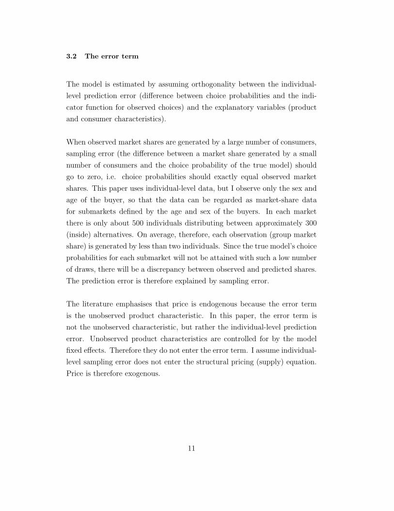
3.2 The error term

The model is estimated by assuming orthogonality between the individual-

level prediction error (difference between choice probabilities and the indi-

cator function for observed choices) and the explanatory variables (product

and consumer characteristics).

When observed market shares are generated by a large number of consumers,

sampling error (the difference between a market share generated by a small

number of consumers and the choice probability of the true model) should

go to zero, i.e. choice probabilities should exactly equal observed market

shares. This paper uses individual-level data, but I observe only the sex and

age of the buyer, so that the data can be regarded as market-share data

for submarkets defined by the age and sex of the buyers. In each market

there is only about 500 individuals distributing between approximately 300

(inside) alternatives. On average, therefore, each observation (group market

share) is generated by less than two individuals. Since the true model’s choice

probabilities for each submarket will not be attained with such a low number

of draws, there will be a discrepancy between observed and predicted shares.

The prediction error is therefore explained by sampling error.

The literature emphasises that price is endogenous because the error term

is the unobserved product characteristic. In this paper, the error term is

not the unobserved characteristic, but rather the individual-level prediction

error. Unobserved product characteristics are controlled for by the model

fixed effects. Therefore they do not enter the error term. I assume individual-

level sampling error does not enter the structural pricing (supply) equation.

Price is therefore exogenous.

11

4 Data

The first subsection describes the data. The assumption that there are no

unobservable differences between variants is central to the paper’s identifi-

cation strategy. Subsection 4.2 discusses how care has been taken to ensure

that trim levels do not cause unobservable differences between engine vari-

ants. Subsection 4.3 discusses further issues concerning trim levels. The

reader who does not care about this issue may skip subsections 4.2 and 4.3.

4.1 Data

The data set is constructed by combining two data sources: new vehicle regis-

trations and price lists from Norway 2000-2007.11 The registration data give

the number of units sold by the sex and age of the buyer.12 I define models

as products of the same brand (e.g. Toyota) and of the same nameplate (e.g.

Corolla). Variants are defined by the engine, as specified by horsepower and

whether it is diesel or not. The sales of a variant is the sum of sales over all

products of a model which are the same in terms of horsepower and fuel type.

(In the literature, for instance in BLP, sales are the sums over products with

the same nameplate.) Prices are list prices, not transaction prices. However,

car importers in Norway have a stated policy of resale price maintenance at

fixed prices.13

11Both were provided by Opplysningsradet for Vegtrafikken AS (the information councilfor road traffic).

12In the sales data, products are defined by the following characteristics: brand, model(nameplate), body type, cylinder volume, horsepower, fuel type, number of seats and drive-wheels (two-wheel drive vs. four-wheel drive). Price lists include the further productcharacteristics length, weight, fuel consumption at mixed driving, airconditioning, numberof collision bags, number of gears, automatic vs. manual gears, whether frontwheel or rear-wheel drive if 2WD, number of doors, and styling package: a set of features (predominantlyaesthetic) summed up by a tag, like ‘sportline’ or ‘comfort’.

13So-called “net prices” or “already-bargained prices” have been standard prac-tice in the industry since around 1998-99, as referred in the country’s largest news-paper Verdens Gang in several articles, “More difficult to bargain”, 30.08.1998,http://www.vg.no/bil-og-motor/artikkel.php?artid=27325 and “Price drop on new cars”

12

Table 1: Descriptive statistics

Means by sex and ageMen Women

year variable meana s.d. 18-35 36-51 52- 18-35 36-51 52-2000 variants 241

models 82priceb 327 157 292 306 276 242 243 225

tax 97 60 88 91 79 68 67 61unit sales 56300 7961 15433 15483 4156 8008 5259

2007 variants 375models 94price 351 194 318 335 310 273 279 245tax 154 127 123 133 119 100 103 86

unit sales 78139 10907 21499 23064 4444 10245 7980

aNot sales-weightedbPrice and tax in 1000s of 2004 kroner, adjusted by CPI.

Table 1 shows summary statistics for the first and last of the eight years in the

data. The data have the sales of 491,853 units, spread over 2397 products,

661 models (giving an average of 3.6 variants per model), 48 age groups and

two sex groups. There is considerable variation along dimensions useful for

identifying the parameters: the number of products across years, average car

tax in different years, and in the purchases of different consumer groups.14

To allow consumers the choice of not purchasing a new car I need an estimate

of the total market size. Since my data are by individual rather than by

household, I could use the total population in each demographic (sex-age)

group to estimate market size. However, on average 98.5% of people do not

buy a new car in a given period. Since the goal is to analyse substitution

patterns for cars, it seems reasonable to focus on the preferences of a more

17.02.1999 http://www.vg.no/bil-og-motor/artikkel.php?artid=45954 .14Differences in average characteristics purchased between groups for a given choice set

reveal the role of demographic variables. Correlations in sales across time within groupswhen the choice set changes (number of products, price, characteristics) reveal the effectof unobserved heterogeneity. Differences in (groupwise) sales within a model reveal themean effects of price and engine characteristics.

13

closely defined group.15 I let the market size of a consumer group be twice

the maximum (across periods in the data) number of people in that group

who bought a new car.

The income distributions conditional on demographic group are from the

population as a whole, not from the potential car buyers as I have defined

them, but this is the best approximation available. I use data from Statistics

Norway on the number of people in twelve sex-age groups belonging to each

of nine income brackets to estimate a kernel-smoothed income probability

density function for each population group.

4.2 Trim level: characteristics that vary within product units

In general, tractability concerns dictate that not all product characteristics

can be included in the econometric model. Typically, for a given product unit

as defined in the econometric model (e.g. nameplate/engine) the consumer

faces a choice of other characteristics (e.g. transmission, leather interior),

which affect the price of the product.

Denote the bundle of characteristics not included the ‘trim level’.16 To assign

one price to each variant it is necessary to choose a trim level for each product.

Denote this the ‘baseline’ trim level. A central identifying assumption in this

paper is that there are no unobserved differences between variants. In the

following I discuss trim levels in some detail in order to show that this issue

does not cause any violation of the restriction on unobservables.

15Also, for a given number of simulation draws, the larger the share of the outside good,the fewer simulation draws will result in a choice of one of the inside alternatives, makingthe simulation of the inside market shares less accurate. The problem could be reducedby oversampling draws that land on inside goods, like BLP do, but it requires an initialestimation with standard simulation techniques, which is difficult to do with any accuracygiven the large computational burden of the model.

16Depending on specific modelling assumptions, my definition of the expression ‘trim’may be wider than common usage.

14

Trim levels do not cause any unobserved difference between variants as long

as three conditions are satisfied: the same set of trim upgrades over the

baseline is available for all variants of a model; the price of upgrades is the

same for all variants; and variants within a model are assigned the same

baseline trim level.17 Together with additively separable utility, this ensures

that consumers choose trim upgrade independently of variant.18 The next

three paragraphs look at how each condition is satisfied.

In some cases not all variant/trim-combinations show up in the price lists.

But examination of car brands’ national web pages show that every engine

variant is available with the full choice of trim levels in almost all cases. The

few exceptions are mostly variants with engine sizes that are outliers relative

to the model range, whose market shares are extremely small, which are not

offered with the cheapest trim levels.

The price lists show that a given trim upgrade almost always costs the same

regardless of engine size. That is, if you have to pay $321 to upgrade from

“basic” to “super” in the 2.0litre variant, you also pay $321 for the same

upgrade with the 2.4litre variant. I use this regularity to infer prices for

variant/trim-combinations that are missing in the data. For the variants

that still do not have a price at the baseline trim after imputing prices in

this way, I reassign sales to nearest neighbour (according to horsepower, and

if tied, fuel type).

The final condition, that all variants of a model are assigned the same baseline

17In fact a weaker condition on availability is sufficient: let Jm

i⊂ Jm be the subset

of variants in model m such that consumer i prefers any variant in Jmi

to any variantin Jm − Jm

iregardless of trim level (even if the variants in the first set have the worst

possible trim and those in the second the best possible). Then it is sufficient that the trimlevel that i prefers is available for all variants in Jm

i, since the availability of trim will not

change the choice of variant. It follows that for instance unavailability of low-end trimwith top-end engine variants is unlikely to contaminate the estimated tastes for enginesize.

18Because of heterogeneity in price sensitivity, this framework is consistent with moreexpensive variants being sold with more expensive trim: people who do not mind payingextra for more horsepower may not mind paying extra for leather seats.

15

trim is up to the researcher as long as the corresponding prices are available.

Since I do not have prices for every variant-trim combination, I chose as

baseline the package for which I have prices for the variants corresponding

to the highest sales (if tied, the cheapest package).19

This discussion shows that the issue of baseline trim does not cause any un-

observed differences between variants. Still the choice of baseline may be

of some consequence. But as I discuss in the next subsection, these conse-

quences are likely to be negligible - especially by comparison to the literature,

where baseline trim also includes engine characteristics.

4.3 Trim level here and in the literature

A consumer’s valuation of the baseline trim level will enter the unobserved

characteristic. Choosing “super” instead of “basic” as baseline for model

m will increase the prices of all variants in m by an equal amount. To

ensure that m keeps its market share δm will adjust upwards. For any given

consumer the effect is exactly the same on all variants, and therefore does not

create unobserved differences between variants. But the choice of baseline

may still have an effect: consumers with a low price sensitivity will substitute

into model m (which has become more attractive since they exchange money

against δ at a higher rate than the average consumer; and an equal amount

with high price sensitivity will substitute out of the model). This may in

principle affect the estimated distribution of price sensitivity. But the effect

of these trim differences is likely to be negligible compared to the effects of

engine characteristics, and model characteristics such as segment and size.

19The raw data have total sales of 523,702 over eight years. For 499,167 of these matchesare found between price lists and sales data. Failures may be due to privately importedobsolete products. Observations that cannot be matched are discarded. The number ofsales for which there is a match between the two data sources, and for which I can find aprice (at a baseline trim level) is is 440,821. Remaining sales are reattributed to nearestneighbours. Finally I discard models with sales in a given year of less than 100 units. Thisreduces the number of products from 3,588 to 2,397 and total sales to 491,853.

16

The choice of baseline is of less consequence in this paper than in the model-

level literature. There are three reasons for this: first, in model-level studies,

trim includes engine upgrades over the baseline engine. Since this makes trim

account for a larger share of utility, the magnitude of the problem is greater.

Secondly, I do not estimate tastes for components of trim, while model-level

studies do, since engine characteristics are in trim. Increasing baseline engine

size therefore changes components of x. This makes consumers with low

tastes for engine size substitute out of the model, which may affect estimates

further. Thirdly, engine upgrades may be correlated (in the population of car

models) with baseline engine sizes (in ways that may depend on the choice of

baseline). Since the engine upgrades enter the unobserved characteristic, ξ,

they may be an additional source of dependence between ξ and x, violating

the orthogonality assumption used in the literature.

5 Estimation

5.1 The objective function

Parameters are estimated by GMM, with moments

gij(θ) = Zij[dij − Pr(j|i, θ, δ(θ))], (10)

where Z is a vector of functions of the explanatory variables.20 dij is one if

consumer i chooses alternative j, zero otherwise. Pr(j|i, θ, δ(θ)) is consumer

i’s choice probability for product j as defined in the model section (equations

(7-9). The model-market fixed effects, δ, are a function of the parameters,

found by setting the aggregate (across consumers) model choice probabilities

equal to model market shares: sm = P (m|θ, δ).

2020 parameters to estimate, 22 instruments: price, price2, kw, kw2, kw ·age, kw · age2, kw · wom, fuelcost, fuelcost2, fuelcost · age, fuelcost ·age2, fuelcost · wom, diesel, diesel · age, diesel · age2, diesel ·wom, length, length2, age, age2, wom, constant.

17

The objective function is

[

n∑

i=1

∑

j∈J t(i)

gij(θ)]′W

[

n∑

i=1

∑

j∈J t(i)

gij(θ)]

, where (11)

W =[

(n)−1

n∑

i=1

∑

j∈J t(i)

Z ′ijZij

]−1,

where J t(i) is the choice set of consumer i, depending on the time period

where i is observed, and n is the number of individuals observed (sum of

market sizes over groups and years). Efficiency could be improved by ap-

proximating the ideal instruments using initial estimates. But because of

the large computational burden, and because the size of the data set makes

efficiency relatively less of a worry I choose to use estimates from (11) as

final.

The vector δ that sets predicted and observed model market shares equal is

found by the BLP contraction mapping.21 Conditional on the parameters,

the model choice probabilities are an average over logit choice probabilities,

like in BLP.

5.2 Simulation and asymptotic properties

The integral with respect to the density of ν and y in the choice probabilities

is computed by a frequency simulator.22 The simulator is not smooth in

the parameters. I analytically integrate over the distribution of the logit

term, but the choice probabilities still contain discontinuous functions of

the parameters: the indicator function 1[j|m], and a max function for every

21δt+1m

= δtm+ log sm − logP (m|θ, δt)

22Using 30 quasi-random draws (scrambled Halton, generated by Matlab’s haltonset) foreach of the 96 consumer groups in each of the 8 years. See Train (2003) for a discussionof Halton draws.

18

model.23 Indicator functions or max functions may change in jumps or not

at all for a given change in their argument, making the same true for the

objective function that depends on them. McFadden (1989) (Theorem 1, p.

1014) shows consistency and asymptotic normality for an estimator like (11)

where g is simulated by a function allowed to have jumps.24 A consistent

estimator for the asymptotic covariance matrix is

ˆAvar(θ) = (G′WG)−1G′W ΛWG(G′WG)−1/n where (12)

G = n−1n

∑

i=1

∑

j∈J t(i)

∇θgij(θ) (13)

Λ = n−1n

∑

i=1

∑

j∈J t(i)

∑

j′≥j

gij(θ)gij′(θ)′. (14)

Berry, Linton, and Pakes (2004) show that under assumptions typical in the

IO demand literature, consistency requires that the number of simulation

draws must grow as the square of the number of products. There are two

reasons that the result does not apply to the model in this paper (so that I

can rely on the results of McFadden (1989)). First, they analyse a situation of

dependence between observations in market-level data, because one market

share depends on the shares of other products. In this paper observations

are individual purchases which do not depend on each other. Secondly, they

23I did not want to use a smoothed simulator (such as a logit-smoothed accept-reject)as discussed in McFadden (1989), because it would effectively remove the feature of mymodel that variants differ only with respect to observed characteristics. In principle onecould create a smooth simulator by decomposing the unconditional probability into a sumof probabilities conditional on which variant is chosen in each model, times the probabilityof the conditioned-on event. If there are M models and each model has V variants, thesum will have MV terms, i.e. approximately 6613.6 = 1.4E+10 in this paper. The com-putational burden is roughly proportional to the number of separate choice probabilitieswhich need to be computed, which is proportional to the number of draws and to thenumber of terms in the sum above. Therefore the computational burden goes down withthe smooth simulator relative to the one I use only if we can reduce the number of drawsby a factor of MV to obtain an equally good simulator. A second alternative would be touse a

24See his assumption A12 p. 1018 for a regularity condition on the behaviour of thesimulator.

19

look at a model where the error term (the unobservable characteristic) is a

nonlinear transformation of the predicted market shares, so that simulation

errors in the choice probabilities will cause a bias. In this paper the error

term is a linear function of the choice probabilities, so that simulation error

cancels across observations and disappears as the number of observations

goes to infinity with the number of simulation draws held fixed.

Because of the irregularity of the objective function I need an optimisation

algorithm that does not require continuity and is robust to local optima. I

use the differential evolution genetic algorithm.25

6 Results

6.1 Parameter estimates

Table 2 shows the estimates from the full model, and table 3 gives variable

definitions and units. The mean taste coefficients, obtained by interacting

with the mean values of the demographic variables, are: horsepower -7.7, fuel

cost 18.7, diesel 0.6, and price -16.6. (For length and the constant for the

outside good the means are contained in δ and therefore unknown.)

The first two do not have the expected signs. Clearly the analysis does not

succeed in disentangling these highly correlated effects. However, since the

variables represent aspects of the same underlying feature, engine size, this

does not necessarily compromise the model’s ability to predict substitution

patterns. A consumer usually cannot change one of these characteristics

without changing the other, and so the effect of having a different engine in

practice works through both characteristics. Gramlich (2009) discusses this

25Developed by Kenneth Price and Rainer Storn, implemented for Matlab in the devec3code, modified to compute population members in parallel. The code can be found onwww.icsi.berkeley.edu/∼storn/code.html.

20

Table 2: Parameter estimates from the full model. 491,853 observations.

product interacted est. s.e.characteristic withhorsepower 4.767 0.007

fuel cost (kroner/km) 4.932 0.007diesel -0.011 0.001

horsepower age -12.303 0.024age sq. -24.685 0.033woman 1.425 0.010

fuel cost (kroner/km) age 12.172 0.021age sq. 30.062 0.042woman -1.604 0.013

diesel age 0.044 0.003age sq. 2.158 0.004woman 0.117 0.008

horsepower std.norm. 0.435 0.005fuel cost (kroner/km) std.norm. -0.167 0.004

diesel std.norm. 1.229 0.015length std.norm. -0.102 0.007

inside good (const.) std.norm. 7.719 0.010pricea α1 2.935 0.014

α2 47.082 0.074α3 3.614 0.007

aThe price coefficient is −[α1 + α2 exp(−α3 · incomei)].

Table 3: Variables and units

Variable Unit mean st.dev. min maxpricea kroner*1E-6 0.34 0.18 0.12 1.87

horsepower kW*1E-2 0.98 0.39 0.37 3.75fuel cost (kr/litre)*(litres/km) 0.77 0.19 0.38 1.86

diesel 1 if diesel, 0 if petrol 0.34 0.47 0 1length metres 4.40 0.32 3.41 5.08ageb age*1E-2 0.50 0.23 0.70

age sq. age squared *1E-4 0.27 0.05 0.49woman 1 if woman, 0 if man 0.29 0 1income kroner*1E-6 0.34 1E-3 3.28

aprice, fuel cost and income in 2004 kroner, adjusted by CPI. 100kroner, abbr. ‘kr’, is about 12 euros or 17 US dollars.

bPersons of age<23 are assigned age 23 and with age>70 assignedage 70.

21

technological frontier in detail.

I regress horsepower on fuel cost over all products to obtain a rough measure

of the technological connection between the two. The slope coefficient is

1.45. So if, starting from the average car, we move to a car with fuel cost

0.1 (kr/km) higher this car would typically have horsepower 0.145 (14.5 kW)

higher. The average consumer would be willing to pay (−7.7 · 0.145 + 18.7 ·

0.1)/16.6 = 0.0454, i.e. 45,540 kroner for this change. To see that this is

roughly in line with market conditions, a regression of price on horsepower

and fuel cost yields coefficients 0.43 and -0.13, respectively. Plugging in the

changes in the two variables, we can expect price to go up by 0.43 · 0.145−

0.13 · 0.1 = 0.0493, i.e. 49,300 kroner.26

6.2 Price elasticities

I compute price elasticities for models by taking derivatives with respect

to a change in the prices of all variants in a model as a percentage of the

sales-weighted mean price. Own-price elasticities range from -3 to -7, and

absolute value tends to increase with price. For semi-elasticities this pattern

is reversed.

Table 4 shows own- and cross-price elasticities (multiplied by 100 for read-

ability) for a sample of models in the 2007 market (found by ordering models

by price and picking every fifth product). Products are ordered by price with

highest price top right. As usual the table shows the elasticity of demand of

the row entry with respect to the price of the column entry. There is a clear

26Slope is 1.69 if I include length and diesel in the horsepower regression. Any charac-teristic in the regression is conditioned on, so in this case the slope is the technologicaltrade-off between fuel cost and horsepower keeping length and fuel type constant. Will-ingness to pay is 34,300 if length and fuel type are kept constant. Including length anddiesel in the price regression gives coefficients of 0.35 and 0.19, resulting in an expectedprice change of 0.35 · .169 + 0.19 · 0.1 = 0.0781, 78,100 kroner. All regression coefficientsare significant to 95% except that (-0.13) on fuel cost in the first price regression.

22

pattern of higher cross-elasticities close to the diagonal (from top-right to

bottom-left), and lower as we move away from the diagonal: cross-elasticities

are higher among products in the same price category.

Variant own-price elasticities are larger in magnitude than those for models,

since they include substitution within the model. Unlike model elasticities,

variant-own price elasticities (and semi-elasticities) decrease in absolute value

with price, presumably because intra-model substitution is larger in cheaper

models.

Table 5 shows variant elasticities for several variants of the same models with

the purpose of highlighting intra-model substitution patterns. The products

were picked by taking a few arbitrary blocks of products adjacent in the

data. Elasticities between variants of the same model can be high, but not

all are, and some are zero. Restricting the idiosyncratic shock to be the same

for all variants of a model permits, but does not impose, high intra-model

elasticities. Substitution is spread less evenly across all products compared

to demand models with idiosyncratic tastes for all products.

23

Table 4: Model elasticities (x100) - w.r.t. price change for all variants of a model

ModelMercedes-Benz E -452 1.4 18.3 0.9 0.6 0.5 2.5 5.3 3.3 0.4 9.5 0.4 3.2 0.9 2.2 0.2

Saab 9-5 3.5 -510 20.3 1.0 0.7 0.5 3.1 6.5 4.0 0.6 12.3 0.6 4.6 1.3 3.4 0.4Toyota RAV4 3.1 1.3 -455 1.2 0.9 0.6 3.9 8.3 5.0 0.7 16.3 0.8 6.6 1.9 5.2 0.6

Jeep PATRIOT 3.0 1.3 24.1 -481 0.9 0.6 4.0 8.5 5.1 0.8 16.7 0.8 6.8 2.0 5.4 0.6Hyundai TUCSON 2.9 1.3 24.4 1.2 -487 0.7 4.3 9.0 5.4 0.8 18.1 0.9 7.6 2.2 6.1 0.7

Kia SPORTAGE 2.5 1.1 19.8 1.0 0.8 -490 5.0 8.5 5.9 1.0 19.5 1.0 9.2 2.6 6.8 1.0Mazda 6 2.0 1.0 18.3 0.9 0.7 0.7 -483 9.2 6.7 1.2 23.4 1.2 12.1 3.4 9.2 1.4

VW TOURAN 2.3 1.1 21.0 1.1 0.8 0.7 5.0 -479 6.2 1.0 22.3 1.1 10.3 3.1 8.9 1.1Volvo V50 2.1 1.0 18.6 0.9 0.7 0.7 5.3 9.1 -488 1.1 22.8 1.2 11.4 3.3 9.2 1.4

Dodge CALIBER 1.7 0.9 18.0 0.9 0.7 0.7 6.0 9.6 7.1 -474 25.3 1.3 13.5 3.9 10.6 1.6VW GOLF’ 1.8 0.9 18.4 0.9 0.7 0.7 5.7 10.0 7.0 1.2 -453 1.3 13.2 4.0 11.4 1.6Hyundai I30 1.6 0.9 18.0 0.9 0.7 0.7 5.9 10.0 7.2 1.2 26.7 -452 13.9 4.2 11.9 1.8

Toyota COROLLA 1.4 0.8 16.5 0.8 0.7 0.7 6.5 10.2 7.7 1.4 29.3 1.5 -441 4.8 13.7 2.1Kia CEE”D 1.3 0.7 16.5 0.8 0.7 0.7 6.3 10.5 7.7 1.4 30.0 1.6 16.4 -432 14.5 2.2

Toyota YARIS 1.2 0.7 16.6 0.9 0.7 0.7 6.3 11.2 7.9 1.4 32.1 1.7 17.4 5.4 -407 2.4Honda JAZZ 0.9 0.6 13.0 0.7 0.6 0.7 6.8 9.7 8.2 1.5 32.6 1.7 19.2 5.8 17.0 -406

Mazda 2 0.8 0.5 12.1 0.6 0.5 0.6 6.9 9.8 8.3 1.6 34.5 1.8 20.6 6.4 18.9 3.5Kia PICANTO 0.8 0.6 15.9 0.8 0.7 0.6 6.3 14.0 8.2 1.4 39.5 2.0 21.8 7.1 24.4 3.1

24

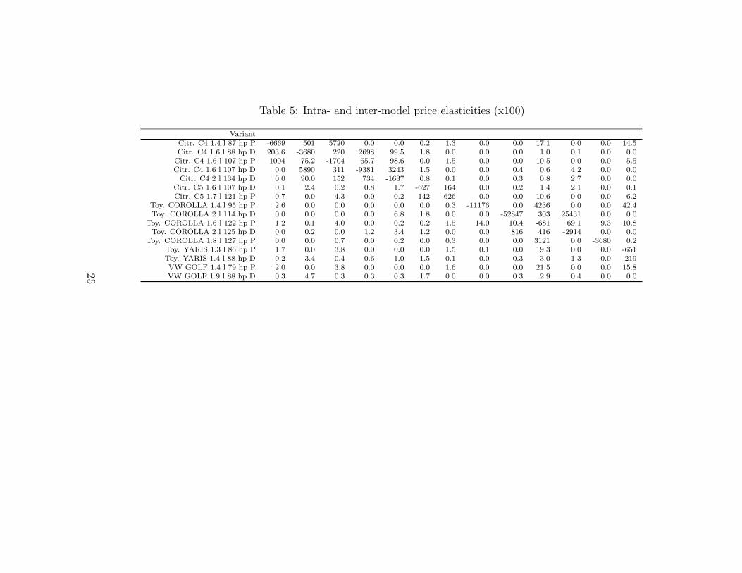
Table 5: Intra- and inter-model price elasticities (x100)

VariantCitr. C4 1.4 l 87 hp P -6669 501 5720 0.0 0.0 0.2 1.3 0.0 0.0 17.1 0.0 0.0 14.5Citr. C4 1.6 l 88 hp D 203.6 -3680 220 2698 99.5 1.8 0.0 0.0 0.0 1.0 0.1 0.0 0.0Citr. C4 1.6 l 107 hp P 1004 75.2 -1704 65.7 98.6 0.0 1.5 0.0 0.0 10.5 0.0 0.0 5.5Citr. C4 1.6 l 107 hp D 0.0 5890 311 -9381 3243 1.5 0.0 0.0 0.4 0.6 4.2 0.0 0.0Citr. C4 2 l 134 hp D 0.0 90.0 152 734 -1637 0.8 0.1 0.0 0.3 0.8 2.7 0.0 0.0

Citr. C5 1.6 l 107 hp D 0.1 2.4 0.2 0.8 1.7 -627 164 0.0 0.2 1.4 2.1 0.0 0.1Citr. C5 1.7 l 121 hp P 0.7 0.0 4.3 0.0 0.2 142 -626 0.0 0.0 10.6 0.0 0.0 6.2

Toy. COROLLA 1.4 l 95 hp P 2.6 0.0 0.0 0.0 0.0 0.0 0.3 -11176 0.0 4236 0.0 0.0 42.4Toy. COROLLA 2 l 114 hp D 0.0 0.0 0.0 0.0 6.8 1.8 0.0 0.0 -52847 303 25431 0.0 0.0

Toy. COROLLA 1.6 l 122 hp P 1.2 0.1 4.0 0.0 0.2 0.2 1.5 14.0 10.4 -681 69.1 9.3 10.8Toy. COROLLA 2 l 125 hp D 0.0 0.2 0.0 1.2 3.4 1.2 0.0 0.0 816 416 -2914 0.0 0.0

Toy. COROLLA 1.8 l 127 hp P 0.0 0.0 0.7 0.0 0.2 0.0 0.3 0.0 0.0 3121 0.0 -3680 0.2Toy. YARIS 1.3 l 86 hp P 1.7 0.0 3.8 0.0 0.0 0.0 1.5 0.1 0.0 19.3 0.0 0.0 -651Toy. YARIS 1.4 l 88 hp D 0.2 3.4 0.4 0.6 1.0 1.5 0.1 0.0 0.3 3.0 1.3 0.0 219VW GOLF 1.4 l 79 hp P 2.0 0.0 3.8 0.0 0.0 0.0 1.6 0.0 0.0 21.5 0.0 0.0 15.8VW GOLF 1.9 l 88 hp D 0.3 4.7 0.3 0.3 0.3 1.7 0.0 0.0 0.3 2.9 0.4 0.0 0.0

25

7 The welfare effects of engine options

This section presents outcomes and welfare effects of a counterfactual exper-

iment where firms are constraint to offer only one engine for each model.27

7.1 The supply-side model

Since I have no data on transactions between car manufacturers, import

companies and dealerships, I follow the literature and treat the supply side as

consisting of vertically integrated car companies selling directly to consumers.

The sales price can be decomposed as

pj = (markupj +MCj)(1 + vat) + taxj (15)

where MC is marginal cost (the incremental cost of producing one more unit

of product j). I assume constant marginal costs within the relevant output

ranges (no economies of scale). tax is the engine tax (an increasing convex

function of horsepower, weight and co2 emissions; in 2007 the tax on average

accounts for 40% of price, ranging from 20 to 70%). markup + MC is the

amount the car company is left with after paying the engine tax and the

value-added tax, vat, of 25%.

I follow the literature and assume that observed prices are a Nash equilibrium

in a game where firms simultaneously choose prices to maximise profits

Πf =∑

j∈Ff

[pj − taxj

1 + vat−MCj ]Msj(p)− Cf , (16)

where Ff is the set of products owned by firm f and M is the size of the

market (summed over all consumer groups). In equilibrium the first-order

27The analysis in this section uses the demand system estimated on the full data set,but markups and the counterfactual are computed only for the 2007 market.

26

conditions for profit maximisation of each product must hold:

0 =sj(p)

1 + vat+

∑

j′∈F (j)

[pj′ − taxj′

1 + vat−MCj′]

∂sj′(p)

∂pj, j = 1, . . . , J (17)

where F (j) denotes the set of products owned by the company which owns

product j. The only unknowns are the marginal costs, which I find by solving

this system of J linear equations in the J unknowns. Once the system of

equations is solved, we know markups and marginal costs.

7.2 Counterfactual

This subsection compares the actual market with equilibrium in a counter-

factual market where each model is offered with only one engine size. I make

two simplifying assumptions: first, that there are no fixed cost investments

involved in expanding the range of engine sizes offered within a model (no

economies of scope).28 Secondly, when companies offer only one engine vari-

ant of each model, they choose the one that generates the highest profits in

the current market.29

Table 6 compares outcomes for the counterfactual single-variant equilibrium

with the outcomes in the actual multi-variant equilibrium.30 Profit increases,

but only by a small amount, 2.4 per cent. In fact markups (average profit

per unit) are marginally reduced, and profit goes up only because the in-

28Often a new variant is created by taking the baseline engine of one of the brand’shigher segment models and putting it in the a lower segment model. Also, developing amore powerful version is less costly than developing an entirely new engine.

29Endogenising the choice of baseline variant would be ideal, but is computationallytoo demanding. It would require the computation of price equilibria for every possibleconfiguration of engine sizes, which is not feasible. Allowing two choices for each firm wouldrequire the computation of 294 equilibria. Relaxing the assumption of perfect informationabout the choices of other firms could simplify the computation of equilibria, but creatinga model of such a game is outside the scope of the paper.

30The numbers for the actual market are based on the model’s predictions of sales. Whilethese predictions are exactly correct for the sales of each model, and therefore aggregatesales, the model does not guarantee a perfect fit at the individual and variant level.

27

Table 6: Market outcomes with single-variant and multi-variant models

i. single-variant ii. multi-variant change % changemodels models

(counterfactual) (actual market)Profitsa 4356 4460 104 2.4Tax revenue 8341 9086 744 8.9from Engine tax 5644 6290 646 5.3from v.a.t. 2698 2796 98 3.6Consumer surplus 63820 66597 2777 4.4Unit sales 75618 77916 2298 3.0Mean priceb 288.7 296.6 7.9 2.7Mean markup 57.6 57.3 -0.3 -0.5Mean horsepower (kW) 87.3 91.6 4.4 5.0

aProfits, tax and consumer surplus in million kroner.bPrice, markup and horsepower are sales weighted.

creased product variety recruits some (3.0%) new consumers who otherwise

would choose the outside good. Making the characteristics of the remaining

engine variants endogenous may change the results, which should therefore

be regarded with some caution. However, choosing the highest-profit vari-

ant of each model, as I currently do, means that chosen variants tend to be

similar for models in the same segments. Models therefore compete head on

in the current counterfactual. Allowing firms to choose characteristics would

open up for more specialisation, and thereby increase markups even more,

reinforcing my conclusion.

Consumers pay more, but are better off, implying that the non-price part

of utility increases more than the disutility of price.31 It has been pointed

out that logit models tend to overestimate the benefit to consumers of prod-

uct variety (see Petrin (2002)), because each new product introduces a new

dimension of differentiation for which some consumers have a very high id-

31In my utility specification income enters the price coefficient linearly, but disposableincome enters only linearly. Total consumer surplus is computed over all consumers,including those choosing the outside good in either case, but these do not experience anychange in consumer surplus since their choice or its attributes do not change. See appendixfor the calculation of consumer surplus.

28

iosyncratic taste. This is not the case here: no new dimension of product

differentiation accompanies the introduction of new engine variants, because

for each consumer, new variants have the same idiosyncratic shock as the

baseline variant of the model. The crowding of characteristics space that

results from multi-variant models is therefore taken into account.

8 Conclusion

I develop a new discrete-choice demand model suitable for a common class

of products which do not fit in existing demand frameworks. I estimate the

model on individual level data, but it could also be used for market level

data, as long as a nonzero prediction error could be justified as sampling

error or in another way.

The model is used to analyse welfare effects of the large number of engine

options offered with car models. The question of what engine variants to

offer if restricting the quality range is related to the recent product-choice

literature, e.g. Mazzeo (2002) and Gramlich (2009). I simplify this ques-

tion by assuming that firms would choose their current highest-profit engine

variant.

References

Ackerberg, D., C. L. Benkard, S. Berry, and A. Pakes (2007):

“Econometric Tools for Analyzing Market Outcomes,” in Handbook of

Econometrics, ed. by J. Heckman, vol. 6. North-Holland.

Ackerberg, D. A., and G. S. Crawford (2006): “Estimating Price

Elasticities in Differentiated Product Demand Models with Endogenous

29

Characteristics,” .

Armstrong, M., and J. Vickers (2001): “Competitive price discrimina-

tion,” RAND Journal of Economics, 32, 579–605.

Bajari, P., and C. L. Benkard (2005): “Demand Estimation With Het-

erogenous Consumers and Unobserved Product Characteristics: A Hedonic

Approach,” Journal of Political Economy.

Berry, S. (1994): “Estimating Discrete-Choice Models of Product Differ-

entiation,” RAND Journal of Economics, 25, 242–262.

Berry, S., J. Levinsohn, and A. Pakes (1995): “Automobile Prices in

Market Equilibrium,” Econometrica, 63, 841–890.

(2004): “Differentiated Products Demand Systems from a combina-

tion of Micro and Macro Data: The New Car Market,” Journal of Political

Economy, 112(1).

Berry, S., O. B. Linton, and A. Pakes (2004): “Limit Theorems for

Estimating the Parameters of Differentiated Products Demand Systems,”

Review of Economic Studies, 71(3), 613–654.

Berry, S., and A. Pakes (2007): “The Pure Characteristics Discrete

Choice Model of Demand,” International Review of Economics.

Dixit, A., and J. Stiglitz (1977): “Monopolistic Competition and Opti-

mum Product Diversity,” American Economic Review, pp. 297–308.

Ellison, G. (2005): “A Model of Add-on Pricing,” Quarterly Journal of

Economics, 120(2), 585–637.

Gilbert, R., and C. Matutes (1993): “Product-line rivalry with brand

30

differentiation,” Journal of Industrial Economics, 41, 223–240.

Goldberg, P. (1995): “Product Differentiation and Oligopoly in Interna-

tional Markets: The Case of the U.S. Automobile Industry,” Econometrica,

63, 891–951.

Gramlich, J. (2009): “Gas Prices, Fuel Effciency, and Endogenous Product

Choice in the U.S. Automobile Industry,” .

Mazzeo, M. (2002): “Product choice and oligopoly market structure,”

RAND Journal of Economics, 33, 1–22.

McFadden, D. (1989): “A Method of Simulated Moments for Estimation of

Discrete Response Models Without Numerical Integration,” Econometrica,

57(5), 995–1026.

Mussa, M., and S. Rosen (1978): “Monopoly and Product Quality,” Jour-

nal of Economic Theory, 18, 301–307.

Petrin, A. (2002): “Quantifying the Benefits of New Products: The Case

of the Minivan,” Journal of Political Economy, 110(4), 705–729.

Rochet, J.-C., and L. Stole (2002): “Nonlinear Pricing with Random

Participation,” Review of Economic Studies, 69(1), 277–311.

Small, K., and H. Rosen (1981): “Applied welfare economics of discrete

choice models,” Econometrica, (49), 105–130.

Train, K. E. (2003): Discrete Choice Methods with Simulation. Cambridge

University Press.

Verboven, F. (1999): “Product line rivalry and market segmentation -

With an application to automobile optional engine pricing,” Journal of

31

Industrial Economics, 47(4), 399–425.

Appendix

A. Hedonic regression

The assumption that there are no unobservable differences between models

is central to the identification strategy of this paper. Results from a hedonic

regression indicate that the assumption holds. Since any unobservable dif-

ference that affects the average consumer’s valuation of a good should show

up in price, I look at how much of price variation can be explained by ob-

served characteristics and model effects. Regressing prices (for all products)

on model(-year) dummies (2397 products, 660 dummies), horsepower, fuel

cost and diesel, cylinder volume and squares of horsepower, fuel cost and

cylinder volume, and a constant gives an R-squared of 0.9913, leaving little

scope for variant-specific unobservables to explain price variation.32 Results

are given in table 7.

32Including further engine-related characteristics (weight, co2 emissions), interactionsand third- and fourth-order terms increases R-squared to as much as 0.9972, but this isopen to charges of overfitting.

32

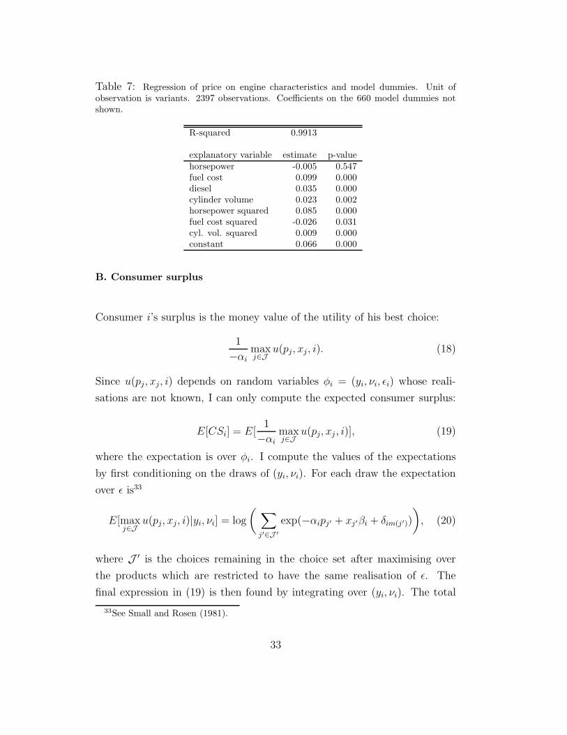
Table 7: Regression of price on engine characteristics and model dummies. Unit ofobservation is variants. 2397 observations. Coefficients on the 660 model dummies notshown.

R-squared 0.9913

explanatory variable estimate p-valuehorsepower -0.005 0.547fuel cost 0.099 0.000diesel 0.035 0.000cylinder volume 0.023 0.002horsepower squared 0.085 0.000fuel cost squared -0.026 0.031cyl. vol. squared 0.009 0.000constant 0.066 0.000

B. Consumer surplus

Consumer i’s surplus is the money value of the utility of his best choice:

1

−αi

maxj∈J

u(pj, xj , i). (18)

Since u(pj, xj, i) depends on random variables φi = (yi, νi, ǫi) whose reali-

sations are not known, I can only compute the expected consumer surplus:

E[CSi] = E[1

−αi

maxj∈J

u(pj, xj , i)], (19)

where the expectation is over φi. I compute the values of the expectations

by first conditioning on the draws of (yi, νi). For each draw the expectation

over ǫ is33

E[maxj∈J

u(pj, xj, i)|yi, νi] = log

(

∑

j′∈J ′

exp(−αipj′ + xj′βi + δim(j′))

)

, (20)

where J ′ is the choices remaining in the choice set after maximising over

the products which are restricted to have the same realisation of ǫ. The

final expression in (19) is then found by integrating over (yi, νi). The total

33See Small and Rosen (1981).

33

(expected) consumer surplus CS in the market is found by summing over

the consumers with characteristics zi for all i:

CS =∑

i

NiE[CSi], (21)

where Ni is the number of people in the market with characteristics zi.

C. Is there price discrimination over engine variants?

This subsection looks at a slightly different, but related issue to that discussed

in section 7.

In competitive markets second-degree price discrimination over quality may

not be possible. Verboven (1999), Armstrong and Vickers (2001), Rochet and

Stole (2002) find that depending on the intensity of competition, markups

may be fixed across quality variants for each firm. Since the theory results

depend on specific assumptions about differentiation and symmetry, I let the

data determine these specifics. The theory models are special cases of the

demand model used in this paper.34

Taking the average of the smallest engine variant over all models (with at

least two variants) gives a markup of 52,800 kroner, while the average of

the biggest variant over all models gives a markup of 83,800 kroner. For

comparison, overall sales-weighted mean markup is 57,300 kroner. Average

percentage markups are 18.36 for smallest variants and 19.75 for biggest

variants. Figure 1 plots markups against horsepower for 9 of the 10 models

in 2007 that have seven or more engine variants, with a line fitted by OLS.

Models are arranged in order of increasing mean price, from left to right,

34My model has many products, each firm offers several models with quality variants,there are several dimensions of taste heterogeneity, and there is an outside good. In thetheory literature there are two firms that each offer one model with quality variants, andthere is one vertical (taste for quality) and one horizontal (taste for models) dimension oftaste heterogeneity. Some theory models do not have an outside good.

34

then top to bottom. Markups clearly increase in horsepower for all models,

with overall markups higher for the more expensive products.

0.5 1 1.5 2

0.05

0.1

0.15

Volkswagen GOLF0.5 1 1.5 2

0.05

0.1

0.15

Opel ASTRA0.5 1 1.5 2

0.05

0.1

0.15

Audi A3

0.5 1 1.5 2

0.05

0.1

0.15

Ford MONDEO0.5 1 1.5 2

0.05

0.1

0.15

Volvo V500.5 1 1.5 2

0.05

0.1

0.15

Mercedes−Benz C

0.5 1 1.5 2

0.05

0.1

0.15

Audi A40.5 1 1.5 2

0.05

0.1

0.15

Bmw 30.5 1 1.5 2

0.05

0.1

0.15

Bmw 5

Figure 1: Markups (in 1e-6 kroner, vertical axis) plotted against horsepower (kw*1e-2,horizontal axis) for models that have seven or more engine variants. Line fitted by OLS.Models arranged in order of increasing price. For the last two products some large enginevariants do not show.

To find the average (over models) effect of engine size on markups within a

model, I regress markups (and percentage markups) on horsepower, horse-

power squared and cubed, a constant, and model dummies. The model

dummies isolate the effect of horsepower, so that higher markups for mod-

els with overall higher horsepower does not contaminate the results. Table 8

shows the results. All higher order terms in horsepower are highly significant.

Figure 2 plots the polynomial functions of markups and percentage markups

obtained from the regression. Markups clearly increase in horsepower within

35

a model, while percentage markups are approximately constant.

Table 8: Results from regression of markups and percentage markups (markup/price)on horsepower, higher order terms of horsepower and model dummies in year 2007. 375observations, 94 model dummies. Coefficients on model dummies not shown.

Explanatory variableshp hp2 hp3 constant

Dependent variablemarkup -0.029 0.056 -0.007 0.038(p-value) 0.205 0.001 0.047 0.000

markup/price -0.214 0.129 -0.024 0.295(p-value) 0.000 0.000 0.000 0.000

0 0.5 1 1.5 2 2.5 30

0.05

0.1

0.15

0.2

0.25

markup/price

markup

Mon

ey (

kron

er*1

E−

6); S

hare

Horsepower (kW*1E−2)

Figure 2: Within-model differences in markups and percentage markups as a functionof engine size. Horsepower in the market ranges from 0.44 to 3.09, sales-weighted mean0.92kW. 10th to 90th percentile (not sales-weighted) is (0.64,1.65)

Consumers who buy larger engine variants of a car model pay a higher pre-

mium over marginal cost than consumers who buy smaller engine variants

of the same model. In this sense there is second-degree price discrimination.

Percentage markups are approximately constant across engine variants.

Several theory papers find that pricing will be cost-plus-fixed-fee, i.e. no price

discrimination. Since my empirical result is different, it is of interest to see

36

what assumptions in the theory literature generates the cost-plus-fixed-fee

results. I simulate some simple duopoly models that relax the assumptions

of the models of Verboven (1999) and Ellison (2005) (by including an out-

side good, making qualities and marginal costs asymmetric, and introducing

heterogeneity in one or both the price and quality parameters).35 I find that

constant absolute markups are the exception rather than the rule.36

35I compute two-firm two-quality Nash equilibria in price in models where the taste forfirms is logit; the price coefficient is either 0.5, U(0,1) or N(0.5,0.5); quality coefficienteither 1 or U(0.5,1.5); marginal costs are (3,4) for both firms, or (1,2)/(3,4); qualities are(7,9) for both, (6,8)/(7,9), or (3,5)/(7,9). If an outside good is included, it has utility -1.5plus logit term. Equilibria are computed by iterating on the best-response functions. Bestresponses are computed using a genetic optimisation algorithm, constraining each firm’shigh quality price to be weakly higher than its low quality price.

36Increasing markups is the most common result, while large asymmetries between firmsmay give decreasing absolute markups for one of the firms. For instance, pricing is nolonger cost-plus-fee in Verboven’s model if we include an outside good. Presumably, theparticipation constraint puts a downward pressure on prices, and more on the low qualityproduct which is the closest substitute to the outside option.

37