Embed Size (px)
Citation preview

1 June 2018 | ESMA50-162-214
Product Intervention Analysis Measure on Binary Options

ESMA • CS 60747 – 103 rue de Grenelle • 75345 Paris Cedex 07 • France • Tel. +33 (0) 1 58 36 43 21 • www.esma.europa.eu
2

3
Table of contents
1 Executive summary ........................................................................................................ 5
2 Analysis of likely impact of different options .................................................................... 6
2.1 Product description and overview of the retail market .............................................. 6
2.1.1 Key product features ........................................................................................ 6
2.1.2 Common characteristics of the market for products offered to retail clients ...... 7
2.2 Summary of problem to be addressed by intervention measures ............................ 7
2.2.1 Geographical scope of problem ........................................................................ 8
2.2.2 Market failure analysis ...................................................................................... 8
2.3 Summary of intervention measures ......................................................................... 8
2.4 Systemic context and market efficiency ................................................................... 8
2.5 Direct impact on firms and investors ........................................................................ 9
2.5.1 Baseline scenario ............................................................................................. 9
2.5.2 Evidence base .................................................................................................. 9
2.5.3 Analysis of intervention options ........................................................................ 9
3 Quantitative analysis .....................................................................................................13
3.1 Summary of main features of the return distribution ...............................................13
3.2 Main results ............................................................................................................15
3.2.1 Notation ...........................................................................................................15
3.2.2 Assumptions ...................................................................................................16
3.2.3 General theoretical results...............................................................................16
3.2.4 Numerical analysis ..........................................................................................17
3.3 General applicability ...............................................................................................21
3.3.1 Different trigger events ....................................................................................21
3.3.2 Continual two-way pricing ...............................................................................23
3.4 Empirical evidence .................................................................................................24
3.4.1 Firm-level data on aggregate client outcomes .................................................25
3.4.2 Evidence on repeated trades ...........................................................................26
4 Annexes ........................................................................................................................27
4.1 Annex I – Proof of general results ..........................................................................27
4.2 Annex II – Application of BSM pricing to up-down options ......................................28

4
5
1 Executive summary
This document summarises and analyses relevant evidence in relation to the provision of
binary options to retail clients. This document complements the European Securities and
Markets Authority Decision of 22 May 2018 to temporarily prohibit the marketing, distribution
or sale of binary options to retail clients in the Union in accordance with Article 40 of
Regulation (EU) No 600/2014 of the European Parliament and of the Council (the Decision),
providing additional detail. This document sets out:
(i) analysis of the impact that different intervention options in relation to binary
options would be expected to have on investors and on firms; and
(ii) a study of the properties of the distribution of returns from investing in binary
options.
In designing the product intervention measures through extended information-gathering and
discussion with National Competent Authorities (NCAs), ESMA considered different
alternatives. Section 2 of this document describes the different options considered and
examines the expected impact of each option. Some impacts are described solely in
qualitative terms, while in other cases quantitative information is available.
On 18 January 2018, ESMA issued a call for evidence on possible intervention measures,
to gather additional information. While most respondents to the call for evidence focused on
issues related to contracts for differences, a minority made reference to binary options.
Section 2 of this document takes these views into account.
Two fundamental features of the return distribution of binary options are especially relevant
from the perspective of possible intervention measures. These are (i) the high levels of risk
involved in binary options, and (ii) the negative expected return of the product. Section 3
examines these features in some detail. A key consequence of the second feature is that
the more often an individual invests in binary options, the more likely he or she is to suffer a
loss on a cumulative basis, and the more likely he or she is to exhaust a given amount of
money available for investing.
Binary options can be structured or provided in different ways. For example, some providers
quote continual two-way pricing, allowing an investor to sell back an option before expiry.
Section 3 sets out simulations based on some more standard products, using examples of
specific numerical payoffs. Importantly, however, the analytical results apply in all cases, as
demonstrated on theoretical grounds. Data presented in section 3 further corroborate the
broad applicability of the analysis. Other data indicate the pertinence of the results relating
to repeated trades.

6
2 Analysis of likely impact of different options
1. This section of the document:
describes what binary options are and describes the retail market for binary options;
explains the key features of the problem that has led ESMA to take action;
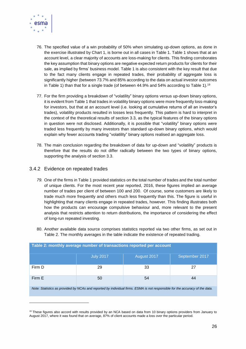
summarises the intervention measures that ESMA is introducing;
examines any potential impact the different intervention options could have on market
efficiency and the wider financial system; and
analyses the expected direct impact of the different intervention options on investors and
on firms.
2. More precise detail on what binary options are, the intervention measure and the problem
addressed are in the Decision alongside which this document is published. 1
2.1 Product description and overview of the retail market
2.1.1 Key product features
3. A binary option is a cash-settled derivative that expires at a pre-specified time. It generally has
two possible outcomes at expiry: either it pays out a fixed monetary amount (the “fixed payoff”),
specified in advance, or it is worth zero (i.e. the investor loses the entire investment). The option
pays out at expiry if a specified event relating to the price of the underlying has occurred. If, at
expiry, the specified event has occurred, the option is said to “finish in-the-money”.
4. Commonly, the specified event that determines whether a binary option pays out is whether the
price of the underlying at expiry exceeds the price of the underlying when the option was issued.
A binary option based on a specified event of this sort is sometimes called an “up-down” binary
option. Box 1 gives an example of an up-down binary option.
1 European Securities and Markets Authority Decision of 22 May 2018 to temporarily prohibit the marketing, distribution or sale of binary options to retail clients in the Union in accordance with Article 40 of Regulation (EU) No 600/2014 of the European Parliament and of the Council.

7
Box 1: example of an up-down binary option
As an example, consider a binary option that has as underlying the level of a large stock index.
The binary option is issued at 9.30am on a particular day. If the level of the index at 4pm that
day is higher than it was at 9.30am, the option pays out, i.e. it finishes in-the-money. In situations
of this kind, the probability of finishing in-the-money is typically around 50%, because a stock
index usually has an approximately even chance of rising over the course of a trading session.
Suppose that the option costs €100 to purchase at 9.30am, and that it pays out €180 if it finishes
in-the-money and zero otherwise. In this case, if the option finishes in-the-money, the investor
makes a net profit of €80. If the option does not finish in-the-money, the investor’s net return is
a loss of €100, i.e. the entire value of the initial investment.
Assuming the probability of finishing in-the-money is 50%, the mathematically expected value of
the option is half of €180, i.e. €90, which is less than the purchase price.
2.1.2 Common characteristics of the market for products offered to retail clients
5. Binary options are often provided OTC to retail clients, and the investor generally has the
provider as counterparty. Counterparty risk is not modelled here.
6. Binary options sold to retail clients usually have very short time horizons, in some cases as
short as a few minutes.
7. Some providers offer continual two-way pricing. This means that retail clients can choose to sell
back binary options they have purchased, before expiry. The amount the investor receives in
return will be somewhere between zero and the fixed payoff. Alternatively, the investor can buy
more of the same binary option. The provider is free to determine the buy price and sell price at
any time, which are not specified in advance.
8. Continual two-way pricing is a feature of the way binary options are provided, as opposed to the
binary options themselves. In other words, the binary option remains the same, contractually,
whether or not two-way pricing is offered.
9. Because binary options offer ‘all or nothing’ payoffs, their return profile is not well-suited to be
used for the purpose of hedging.
2.2 Summary of problem to be addressed by intervention measures
10. Retail clients have received poor outcomes from investing in binary options. Binary options
provide investors with a negative expected return, with no appreciable offsetting benefits other
than facilitating speculation. As a result, a large majority of retail client accounts lose money in
aggregate (even though some investors may make profits, especially in the short term).

8
2.2.1 Geographical scope of problem
11. The issue has an EU-wide impact on retail client protection, as evidenced by investor outcomes
in several Member States. In many cases, retail customers trade binary options with providers
that operate cross-border.
2.2.2 Market failure analysis
12. The problem is due in part to informational asymmetries. A clear majority of retail clients lose
money, indicating that retail clients as a group overestimate the net returns they are likely to
receive and do not understand the intrinsic features of these products.
2.3 Summary of intervention measures
13. As set out in the Decision, ESMA is imposing a temporary (three-month) prohibition on the
marketing distribution or sale of binary options to retail clients.
2.4 Systemic context and market efficiency
14. There is no evidence of systemic risk from prohibiting the provision of binary options to retail
clients in the EU. The intervention is expected to have no discernible impact on prices or liquidity
of underlying assets or of other derivative contracts. Many firms providing binary options to retail
clients are believed not to generally hedge their exposure using options in institutional markets,
and so there is no evident channel through which any material financial shock could be
propagated to financial markets more broadly. Additionally, while ESMA does not have a
conclusive estimate of the size of the retail market for binary options in the EU, data on the
numbers of clients in different jurisdictions and average client losses suggest that the order of
magnitude of volumes of retail binary options is small compared with institutional options
markets. Data reported by NCAs referred to in the Decision suggest an approximate upper
bound on numbers of accounts in the EU to be around 500,000. Assuming an average client
loss of EUR 500 annually – which is of the order of average estimated losses estimated by
NCAs – yields an approximate upper bound on industry net revenues to be EUR 250 million. If
average net revenue for binary options providers is 2% of contract size (a conservative estimate,
in the context of estimating an upper bound on total volumes) then total annual volumes in binary
options held by retail clients in the EU are unlikely to exceed EUR 12.5 billion. This figure is a
very small fraction of total amounts outstanding in institutional options markets, which exceed
EUR 10 trillion according to data from the Bank of International Settlements.2 Moreover, the
total annual volumes of binary options traded by retail clients are likely to be far higher than the
amount outstanding at any point in time, as the typical term of binary options is very short.
2 Source: Bank of International Settlements, data update 2 November 2017. Latest data update is available at https://www.bis.org/statistics/d5_1.pdf

9
2.5 Direct impact on firms and investors
15. The following part of section 2 deals with the costs and benefits that the relevant intervention
options considered by ESMA in developing the temporary prohibition would be likely to have on
investors and on firms. 3 The analysis includes both quantitative and qualitative evidence.
2.5.1 Baseline scenario
16. The baseline scenario against which the impacts of the intervention options are assessed is the
regulatory regime to which the market is subject is in place prior to the commencement of the
intervention measures in question. In particular, firms are assumed in the baseline scenario to
be subject to the requirements of MiFID II / MiFIR, all other applicable EU Directives and
Regulations and all national rules in force. For example, the baseline scenario includes the bans
on commercialisation or advertising of complex products (including binary options) in place in
Belgium and in France, as these policies are in place when the ESMA intervention comes into
force.
2.5.2 Evidence base
17. In respect of the costs and benefits of the intervention measure to retail clients, the evidence
base includes detailed quantitative analysis, whereas in respect of the costs and benefits to
firms, the evidence is mostly qualitative.
18. Figures on client returns provided by NCAs are based on samples of client accounts as reported
by firms. Pricing information used to simulate examples of expected returns for investors taken
from firms’ public websites and the exact numerical estimates (as opposed to the quantitative
analysis of the structural properties of the return distribution) should be regarded as illustrative
only.
2.5.3 Analysis of intervention options
19. In all cases, the options described below assume that binary options traded on a trading venue
are in scope for the measures. Some respondents to the call for evidence argued that binary
options traded on a trading venue, whether or not securitised, should be excluded from the
scope of the measures. However, the features and characteristics of binary options, which are
the fundamental source of the identified detriment to retail clients (and the subsequent
significant investor protection concerns), remain the same whether or not these products are
traded on a trading venue. In other words, binary options on a trading venue would still present
a negative expected return to investors, while offering a payoff structure that is poorly suited to
3 Impacts on investors should be interpreted while bearing in mind the objective to limit the significant investor protection concern arising from the sale, distribution or marketing of binary options. In particular, it is important to note that aggregate monetary total costs and benefits, where obtainable, do not necessarily equate to aggregate detriment, e.g. in the following respects. (i) Some consumers may not expect certain costs, or understand the risk that the costs will materialise. If the costs do then materialise, the resulting detriment may be greater than if the consumers had anticipated the risk. (ii) The wealth and liquidity of consumers bearing costs also have a bearing on detriment. For example, a consumer whose losses exceed his or her cash balances with a firm and is unable to settle his or her account is likely to suffer considerably more detriment than an investor suffering a loss of the same size but which is covered by his or her cash balances. (iii) The distribution of costs on consumers is relevant to detriment. Other things equal, if a given aggregate loss falls on a smaller number of investors, this may cause more overall detriment than the same aggregate loss spread over a larger number of investors.

10
the purpose of hedging or other economic functions that could form a compensating benefit.
Notably, these properties hold true at any time prior to the expiry of the option. The existence of
any secondary market in binary options, therefore, does not change the fundamental
characteristics that cause detriment to retail clients.
Intervention
objective
Address the significant investor protection concerns arising from the sale,
distribution or marketing of binary options.
Option A Prohibit the marketing, distribution or sale of binary options to retail clients.
Option B Restrict the provision of binary options to retail clients, e.g. impose limits on
the amount of money that a client can invest per trade or per client, or impose
a minimum term.
Option C Prohibit the marketing, distribution or sale of binary options to all clients.
Preferred Option Option A. As detailed below, there are common intrinsic features of binary
options which are the fundamental source of detriment to retail clients.
Therefore, limiting the range of binary options to which measures would apply
(option B) is not warranted. On the other hand, the analysis conducted by
NCAs and ESMA has focused on the significant investor protection concern
arising from the detriment to retail clients and therefore option C is not selected
at this stage.
Option A Prohibit the marketing, distribution or sale of binary options to retail clients
Benefits Retail clients would no longer suffer any monetary losses or other detriment in
connection with binary options. They would be comprehensively protected
from the high levels of risk arising from a structurally negative expected return
product, a type of product which, in addition, is poorly suited to hedging and
investment purposes.
Costs to regulators The measure would need to be enforced and monitored. Monitoring costs
would be lower than option B, however, since NCAs would not need to assess
the features of binary options sold, distributed or marketed to retail clients.
Compliance costs
Firms would forego all future revenues arising from the provision of binary
options to retail clients. Firms whose sole business is providing binary options
could exit the market or would have to turn to other products (or to focus their
offer to non-retail clients only). Firms who provide other products in addition to
binary options would need to cease providing binary options, and as a result
some such firms may exit the market.

11
Some costs would be involved in updating IT systems. CMC Markets, in its
response to the call for evidence, estimated the costs incurred by the firm in
this respect to be around GBP 16,000.
The cessation of losses by investors would approximately balance, in
aggregate monetary terms, the lost revenue by firms.
Other costs A minority of retail clients make positive net returns in the baseline scenario.
Such positive net returns would not accrue to investors under options A or C.
Some respondents to the call for evidence indicated that binary options on a
trading venue should be excluded from the scope of the measures. However,
the features and characteristics of binary options, which are the fundamental
source of the identified detriment to retail clients, remain the same whether or
not these products are traded on a trading venue, and any time prior to the
expiry of the option. The existence of a secondary market, therefore, does not
change the fundamental characteristics that cause detriment to retail clients,
just as the possibility of two-way pricing offered by OTC providers does not
alter such characteristics.
Option B Restrict the provision of binary options to retail clients, e.g. impose limits on
the amount of money that a client can invest per trade or per client, or impose
a minimum term.
Benefits Restrictions designed to limit the frequency (via a minimum term) or amount
of investment by a client would aim at reducing the risk of substantial
detriment. However, the analysis of the return distribution detailed in section 3
applies regardless of the initial investment. In particular, investors would still
face a negative expected return, which would come in the absence of providing
any compensatory benefits such as hedging. This would limit the benefit of the
intervention option.
Costs to regulators The measure would need to be enforced. Either a per-trade or per-account
monetary limit or a minimum term requirement would require national
authorities to monitor the detail of binary options offerings, which would incur
higher costs for regulators than options A or C.
Compliance costs Firms would incur one-off costs in changing their platform software and their
terms and conditions and on-going costs to ensure ongoing compliance
Some costs would be involved in updating IT systems, as for options A or C.
Other costs A minority of retail clients make positive net returns in the baseline scenario.
These investors would be constrained, but would still be able to trade binary
options under option B, unlike under options A or C.

12
Option C Prohibit the marketing, distribution or sale of binary options to all clients
Benefits All clients would no longer suffer any monetary losses or other detriment in
connection with binary options. They would be comprehensively protected
from the high levels of risk arising from a structurally negative expected return
product, a type of product which, in addition, is poorly suited to hedging or
investment purposes.
Extending the prohibition of marketing, distribution or sale of binary options to
all investors would be warranted by the described features of the products and
would consequently also benefit non-retail clients (professional clients and
eligible counterparties). On the other hand, ESMA has no evidence that such
clients actually use binary options. Additionally, non-retail clients would be less
likely to invest in binary options without understanding the return profile and
the pricing structure of these complex products, in contrast to retail clients,
limiting the amount of any potential protection that a prohibition would provide
such clients.
Costs to regulators The measure would need to be enforced and monitored. Monitoring costs
would be lower than under options A or B due to the complete ban of binary
options for all categories of clients.
Compliance costs
Firms would forego all future revenue arising from the provision of binary
options. Firms whose sole business is providing binary options would exit the
market or would need to turn to other products. Firms who provide other
products in addition to binary options would need to cease providing binary
options, and as a result some such firms may exit the market.
Some costs would be involved in updating IT systems, as for options A or B.
The cessation of losses by investors would approximately balance, in
aggregate monetary terms, the lost revenue by firms.
Other costs A minority of retail clients make positive net returns in the baseline scenario.
Such positive net returns would not accrue to investors under options A or C.

13
3 Quantitative analysis
20. This section of the document:
provides an overview of the features of the return distribution for retail clients in binary
options;
states the main results mathematically; and
presents graphical simulation results and discusses relevant empirical data.
21. Section 3.1 discusses the main features of the return distribution. Section 3.2 then formally
presents the main results. For clarity, graphs of simulation results accompany some of these
results. The simulations use specific examples of payoff structures.
22. Section 3.3 demonstrates the general applicability of the results. In particular, it shows that the
results are robust across different types of payoff structure – including where the strike price
differs from the initial price of the underling – and that they hold whether or not the provider
offers continual two-way pricing.
23. Section 3.4 provides relevant data and information from firms, and concludes that the available
empirical evidence supports the (largely theoretical) modelling exercise.
24. A further, minor, robustness check is provided in Annex II, in relation to the assumed 50% win
likelihood assumed when modelling up-down options. The robustness check is performed by
using the Black-Scholes-Merton (BSM) pricing model. The reason that the check is of minor
importance is that, as established in section 3.3, the 50% likelihood is not critical to the results.
However, the check provides evidence that the specific modelling of up-down options reflects
the actual return distribution for those options.4
3.1 Summary of main features of the return distribution
25. The theoretical distribution of returns from binary options has the two following fundamental
properties.
i. The high level of risk involved.
ii. The negative expected return of the product.
26. The first feature is the high level of risk that the investor takes on in purchasing a binary option.
A general feature of all binary options is that an investor risks losing his or her entire investment.5
4 This, in turn, corroborates the estimate for the negative expected return of around −10% for the up-down binary option modelled in section 3.2.2, which is based on a market provider’s quote In other words, there is evidence that some binary options are sold at a large expected mark-up compared to fair value. However, the size of the mark-up as a potential source of investor detriment is not central to the case made for the intervention measure.
5 The main quantitative analysis assumes that if option finishes out of the money it pays out zero. There is a small technical caveat to this assumption, which has no impact on the results. For more details, see the discussion in section 3.2.1.

14
As mentioned above, for a standard up-down binary option the probability of this happening is
around 50%.
27. Even a single trade therefore involves a high level of risk. Risk alone is not necessarily a source
of investor detriment, if an investor takes on risk because he or she reasonably expects higher
returns, for example. However, binary options do not compensate investors for the risk they
take on by offering commensurate expected rewards. For this reason, the level of risk
represents a source of investor detriment (and therefore a significant investor protection
concern).
28. The second feature, the negative expected return of a binary option for the investor, refers to
the mathematical expectation of the return on the investment. It means that if the option’s fixed
payoff is multiplied by the probability of finishing in the money, the result is less than the initial
amount invested. Taking the example in Box 1 in section 2.1.1, the product has a 50% chance
of finishing in-the-money, and if it does so, the investor receives €180. The expected net value
of the binary option is therefore half of €180, i.e. €90. The initial investment of €100 is greater
than the expected net value of the option, which means that the investor’s expected return is
negative.
29. The negative expected return does not necessarily require that the investor is more likely to lose
than to win. In many cases, such as for up-down binary options, the probability of winning is
around 50%. But in other cases, the probability may be different. Nonetheless, the expected
return will be negative. Investors must face negative expected returns, or providers’ business
model would not be profitable
30. In the context of binary options, the negative expected return is another important source of
detriment and applies to all binary options. While the existence of a negative expected return
on an asset or financial instrument is not in itself grounds for concern (for example, an insurance
contract is valuable to a risk-averse investor despite having a negative expected return), binary
options do not provide any compensating benefit in terms of economic functions such as
insurance, hedging or investment. Unlike financial investments, the contracts are typically very
short term and do not offer participation in the growth in value of the underlying. Unlike vanilla
options, which are often used for hedging purposes, binary options provide a fixed payoff if a
specified event occurs. In contrast, the payoff of a typical option is contingent on the change in
the price of the underlying once the option is in the money (i.e. the payoff is variable). This
inherent feature of the products limits the value of the product as a hedging tool, whereas other
kinds of option have been used to smooth out or limit the price of an asset to which a firm or an
investor has direct exposure.
31. An important consequence of the fact the investor faces a negative expected return is that the
more often he or she invests, i.e. the more binary options he or she bets on, the greater the
probability of suffering a loss on a cumulative basis. This fact ties in to a simple interpretation of
the expected value of a gamble as being the long-run average outcome of many repeated trials.
32. Relatedly, repeated investment (i.e. placing a series of bets) also increases the probability that
an investor entirely depletes a given amount of money available for investing.

15
3.2 Main results
3.2.1 Notation
33. In stating the payoffs of an option, it is simplest to normalise by assuming an investment of 100
units of currency. Let the payoff vector (𝑎, 𝑏) denote the payoffs for an investor, where:
the first entry, 𝑎, denotes the gross payoff if the option does not finish in-the-money;
and
the second entry, 𝑏, denotes the gross payoff if the option finishes in-the-money
34. For example, the payoffs of the binary option in Box 1, which pays out €180 (gross) on a €100
investment, and zero otherwise, are denoted (0 , +180).
35. This notation denotes only the payoffs, and not the probability distribution over the payoffs. This
means that simply comparing two binary options’ respective payoff vectors does not reveal
which has the higher expected value, unless the probability of finishing in-the-money is also
known. For example, if two options have identical payoff vectors, but one is 55% likely to finish
in-the-money while the other only has 45% likelihood, the former has a higher expected value.
36. For generality, the notation allows for the possibility that 𝑎 ≠ 0. Some providers offer options
that pay a small amount if the option does not finish in-the-money. This offering is equivalent to
the investor making a small payment to the provider that is due to be returned unconditionally,
alongside purchasing an option that pays zero if it does not finish in-the-money.6 While it is
convenient to assume that 𝑎 = 0 for the theoretical results in this analysis, the results in fact
hold more generally.
37. Other notation used is as follows. Define 𝑝 to be the probability of finishing in the money, so that
the expected value of payoff vector (𝑎, 𝑏) is given by (1 − 𝑝)𝑎 + 𝑝𝑏 = 𝑝𝑏 (recalling that 𝑎 = 0).
The expected return 𝑟(𝑎, 𝑏, 𝑝) – expressed as a proportion of the initial investment of 100 – is
then as follows: 7
𝑟(𝑎, 𝑏, 𝑝) =(1 − 𝑝)𝑎 + 𝑝𝑏 − 100
100=
𝑝𝑏
100− 1
38. For clarity, the notation hereafter omits the arguments when denoting the expected return, i.e.
simply writes it as 𝑟.
6 Abstracting away from counterparty risk, this can be seen mathematically as follows. Consider a binary option with payoff vector (+5, +175). The payoff vector can be written (+5 , +175) = (0 , +170) + (+5 , +5), i.e. a binary option with a gross payout of 170 and zero otherwise, plus a certain return of 5.
7 The normalisation of assuming an investment of 100 makes no difference to the results. One way to see this is that the definition of 𝑟 can simply be made scale-invariant by allowing for the initial investment to be a variable 𝑦. In this case, if (𝑎, 𝑏) is the payoff
vector for an investment of 100, then (𝑦
100𝑎 ,
𝑦
100𝑏) =
𝑦
100(𝑎 , 𝑏) is the payoff vector from investing 𝑦. The return is then given by
𝑟 =𝑦
100[(1−𝑝)𝑎+𝑝𝑏]−𝑦
𝑦= (1−𝑝)𝑎+𝑝𝑏−100
100, as before.

16
3.2.2 Assumptions
39. The results that follow are based on the following key assumptions:
Assumption 1: 𝑟 < 0. This assumption is justified by the simple fact that offering binary
options must yield expected profit for the provider, or the business model used by providers
would not be sustainable.
Assumption 2: in any series of investments in binary options, the outcome of each
investment (i.e. whether it finishes in-the-money) is realised independently of the outcomes
of the other investments.
3.2.3 General theoretical results
40. The long-run effects of repeated investments in any binary option (for which 𝑟 < 0 ) are
summarised in the following theoretical results.
a) If an investor makes a large number of investments, then the investor is unlikely to make a
positive overall return. Formally, the probability that the sum of the investor’s returns is
positive will tend to zero as 𝑛 tends to infinity.
b) If an investor has a limited amount of cash available to invest in binary options, and makes a
large number of investments, then the investor is likely to lose all the cash. Formally, this
result is implied by the fact that the probability that the sum of the returns is less than any
given finite number will tend to one as 𝑛 tends to infinity.8
41. These results are proved in Annex I. Chart 1 illustrates the properties graphically, for the
example payoff vector (0 , +180). The horizontal axis denotes the number of trades and the
horizontal axis represents the probability mass density of the distribution. It can be seen from
the chart that the expected return (mean) of the distribution linearly decreases in the number of
trades, as – 𝑛𝑟. The proportion of each curve lying below a given constant – for example, zero
on the horizontal axis – is also seen to decrease as the number of investments 𝑛 increases.
8 The reason the formal statement is in fact a sufficient (but not a necessary) condition for the first sentence in result (b) is as follows. An available cash sum is represented as some finite number. The formal statement says that a large series of returns will converge in probability to less than that number, i.e. the cash will be depleted in the long run. However, it is also possible that a short series of returns may, through chance, deplete the entire cash sum. As the cash sum is a liquidity constraint, trading would then cease with the cash sum exhausted.

17
Chart 1: distribution of aggregate return from selected numbers of repeated investments of 100 in binary
options with payoff vector (0 , +180) when 𝑝 = 0.5 and investment outcomes are realised independently
3.2.4 Numerical analysis
42. The theoretical results are very general, applying to all binary options (assuming negative
expected returns). However, by the same token, they are also abstract. For concreteness a
specific worked example is first presented, before turning to graphical illustrations for different
numerical payoff vectors and win probabilities.
3.2.4.1 Worked example
43. Consider the payoff vector of Box 1, (0 , +180). As the present focus is an up-down option, set
𝑝 = 0.5. As noted in Box 1, 𝑟 <90−100
100= −10% < 0.
44. The expected return after making 𝑛 ≥ 0 such investments is simply 𝑟 × 𝑛 = −0.1𝑛 < 0.
45. The distribution of returns after making 𝑛 ≥ 0 such investments is given by the binomial
distribution. Specifically, the probability that the investor wins exactly 𝑘 times from 𝑛
investments is given by
𝑃𝑟(𝑘; 𝑛, 𝑝) = (𝑛𝑘
) 𝑝𝑘(1 − 𝑝)𝑛−𝑘
where (𝑛𝑘
) ≡𝑛!
(𝑛−𝑘)!𝑘! .
0%
2%
4%
6%
8%
10%
12%
14%
16%
18%
20%
-8,000 -6,000 -4,000 -2,000 0 2,000
20 investments 50 investments 100 investments 250 investments
Note: Probability mass density, according to binomial distribution, of aggregate net return for sel ected total numbers of i nvestments made, whereeach invetment is of size 100 and the payoff vector is (0 , +180). Each investm ent is assumed to finish in-the-money with a probability of 50%and all outcomes are assumed to be realised i ndependently. Plotted distributions are truncated for clarity (i) for horizontal axis val ues below -
8000 and above +3000, and (ii) for vertical axis values below 0.001%.Sources: AFM, ESMA.

18
46. As 𝑝 = 0.5 in this case, the expression simplifies to
𝑃𝑟(𝑘; 𝑛, 0.5) = (𝑛𝑘
) 0.5𝑛
47. Let the function 𝑞(𝑛) > 0 denote the minimum number of wins an investor needs from 𝑛 > 0
investments such that the aggregate return is positive. In other words, for given 𝑛, 𝑞(𝑛) is the
smallest integer such that the following inequality holds.
𝑞(𝑛)𝑏 > 100𝑛
48. Suppose a customer makes 20 investments, so that 𝑛 = 20. The overall number of wins is
randomly determined, and must lie between 0 and 20. To work out the investor’s probability of
winning overall, the first step is to work out the minimum number of wins out of 20 investments
consistent with an overall win, when the amounts won and lost are added up. In other words, it
will be necessary to determine 𝑞(20).
49. It turns out that 𝑞(20) = 12. This can be seen by first considering what happens when the overall
number of wins happens to be 11, which yields a net cumulative return of 9 × (𝑎−100
100) + 11 ×
(𝑏−100
100) = 9 × (−1) + 11 × 0.8 = −0.2 < 0.
50. In other words, if an investor make 20 investments, each of €100, in the binary option in
question, then if there are 11 wins and 9 losses, the investor loses 20% of the initial stake, or
€20.
51. If the overall number of wins happens to be 12, the net cumulative return is €160. This is
because the net cumulative return, as a proportion of a €100 investment, is 8 × (−1) + 12 ×
0.8 = +1.6 > 0.
52. The binomial distribution then implies that the probability of winning on a cumulative basis after
20 investments is given by
𝑃𝑟𝑜𝑏(𝑜𝑣𝑒𝑟𝑎𝑙𝑙 𝑤𝑖𝑛) = ∑ (20𝑘
) 0.520
20
𝑘=12
which is around 25%. This implies that the probability of losing overall is around 75%.
53. A similar procedure yields a lower bound for the probability of depleting a given amount of cash
available for investment.9 For instance, suppose the investor places 20 trades each of €100. If
the number of wins happens to be 6, then the investor loses €920, as
14 × (−1) + 6 × 0.8 = −9.2
9 The reason that the procedure determine a lower bound for the probability of depleting available cash, rather than the actual probability, is that it assumes the investor will make all 20 investments. It excludes, for instance, sequences in which that the investor’s first 10 investments all lose, but the total number of subsequent wins is greater than 5. As by hypothesis €1000 is the total available budget for investment, such sequences represent cases where the investor’s entire budget would be depleted. For present purposes, however, the lower bound is instructive, as the aim is simply to illustrate general properties through specific numerical examples.

19
54. If the number of wins happens to be 5, then the overall return is a loss of €1100, as
15 × (−1) + 5 × 0.8 = −11
Hence the probability of entirely depleting a €1000 budget for investment satisfies the following
inequality.
𝑃𝑟𝑜𝑏(𝑒𝑥ℎ𝑎𝑢𝑠𝑡 €1000 𝑏𝑢𝑑𝑔𝑒𝑡 ) > ∑ (20𝑘
) 0.520
5
𝑘=1
i.e. the probability of exhausting the budget is greater than 2%.
3.2.4.2 Graphical simulation results
55. Using the procedure outlined in the worked example above, it is possible to simulate overall loss
probabilities for any given payoff vector, for different numbers of trades. Chart 2 presents overall
loss probabilities for sequences of €100 investments in binary options with payoff vector
(0 , +180) and win probability 𝑝 = 0.5, where investment outcomes are realised independently.
The length of the sequence 𝑛 varies on the horizontal axis. The loss probabilities plotted are
specifically (i) the probability of overall loss, after 𝑛 investments; and (ii) the probability of losing
at least €1000, €2000 and €3000 respectively.10
10 As each investment is of size 100, a sequence length of 𝑛 = 50, for instance, represents a total gross investment of 5000.

20
Chart 2: simulated probabilities of cumulative loss exceeding given amounts for repeated investments
of 100 in binary options with payoff vector (0 , +180) when 𝑝 = 0.5 and investment outcomes are
realised independently
56. While the actual probabilities plotted in Chart 2 are only for integer values of trade numbers, the
results are plotted with lines in between these points for visual clarity. To interpret the graphical
results, note first that for a single trade, an overall loss requires that the investor lose that single
trade; the overall loss probability therefore starts equal to 𝑝 for 𝑛 = 1. For an up-down option, a
negative expected return implies that one win and one loss from two investments results in an
overall loss, and so the only way to win overall for 𝑛 = 2 is for both investments to pay out. This
is why the overall loss probability jumps to 75% for 𝑛 = 2. For the first few odd values of 𝑛, there
needs to be one more loss than wins for an overall loss, whereas for even values of 𝑛, there
need to be two more, which explains the “zig-zag” pattern. Periodically, the proportion of losses
needed for an overall loss reduces by one for both odd-length and even-length sequences,
which explains the less frequent, larger step increases in loss probability as 𝑛 increases. Finally,
note that all the plots form a family of “S”-shaped curves (most clearly seen in the case of
probability of overall loss of at least 1000, given the scale on the horizontal axis), whose values
will converge on 100% for large 𝑛.
0%
10%
20%
30%
40%
50%
60%
70%
80%
90%
100%
0 10 20 30 40 50 60 70 80 90 100 110 120 130 140 150 160 170 180 190 200 210 220 230 240 250
Number of times option is traded
Probability of overall loss Probability of overall loss of at least 1000
Probability of overall loss of at least 2000 Probability of overall loss of at least 3000
Note: Loss probabilities are those of an investor with unconstrained liquidity. For a liquidity-constrained investor, simulated values are lower bounds. Binaryoption simulated has gross payoffs of 180 when finishing in-the-money and zero otherwise, on an investment of 100. Each trade is assumed to finish in-the-money with probability of 50%, with all outcomes realised independently. Probabilities are plotted for integer values on horizonal axis, with lines joining thesepoints for clarity.Sources: AFM, ESMA

21
3.3 General applicability
57. The analysis of section 3.2 focused on standard up-down options. For up-down binary options,
the specified event on which payoffs are conditioned (the “trigger event”) is that the price of the
underlying at expiry exceeds the price when the binary option was issued.11 This section shows
that the properties of the return distribution identified in section 3.2 hold for all binary options.
3.3.1 Different trigger events
58. Some providers offer binary options with different kinds of trigger event. The use of terminology
in this context can vary between firms. Beyond the standard up-down binary option, other types
of trigger event include, but are not limited to, the following.12
The option finishes in the money if the price of the underlying at expiry exceeds the
strike price, where the strike price differs from the initial price. Some providers call this
a “ladder” option.
The option finishes in-the-money if the price of the underlying exceeds the strike price
at any time before expiry.13 Some providers call this a “touch” option.
The option finishes in-the-money if the price of the underlying is within a certain range
at expiry. The payoff of a target option is therefore mathematically equivalent to that of
two up-down binary options, a short option with a strike price equal to the higher end of
the range and a long option with a strike price equal to the lower end of the range.14
Some providers call this a “range” option.
59. Section 3.2 focused on modelling up-down binary options, as these are routinely offered by
many binary options providers and provide a clear reference point. Larger providers tend to offer
other types of binary option alongside up-down binary options.
60. Because the underlying event can vary, the value of the other types of binary options may be
especially hard for retail clients to understand. For instance, a “touch” option is more likely to
finish in-the-money than an up-down option with the same underlying, strike price and expiry
time. The reason is intuitive: for the touch option to pay out, the price of the underlying simply
needs at some point during the term to “touch” (or cross) the relevant threshold, rather than to
be at or above the threshold at expiry. However, estimating exactly how much more likely the
11 This description assumes a long option. If the option is short rather than long, the option is in-the-money if the price of the underlying is less than the initial price.
12 Some offerings may involve a series of trigger events, with more than one fixed payoff depending on which events in the series occur. Such offerings are in effect a sequence of dual-payoff binary options.
13 Unlike the other types of product listed, such an option would therefore probably be priced as an American option, rather than as a European option.
14 For example, suppose such an option has a gross payoff of +50 if and only if the underlying price ends between €35 and €36, and 0 otherwise. This has the same payoff as the following pair of options: (i) a long binary option that has a gross payoff of +25 if the underlying price ends above €35 and -25 otherwise; (ii) a short binary option with a gross payoff of +25 if the underlying ends below €36 and -25 otherwise. Taking the payoffs of the pair together, the investor receives +25-25=0 if the price of the underlying ends below €35, 25+25=50 between €35 and €36, and -25+25=0 if the price of the underlying ends above €36.

22
touch option is to pay out than its up-down equivalent is complicated, because it depends not
just on where the price ends up but what path it takes before expiry.
61. For the purposes of this analysis, attention is focused on the fundamental properties of the
return distribution of any given binary option – namely the high level of risk and the negative
expected return – and the effects of repeated trades. Importantly, these implications hold
generally. The reason is that in all cases, a binary option pays out a fixed monetary amount with
some given ex-ante probability.
62. To illustrate the fact the results extend beyond up-down options to all binary options regardless
of the type of trigger event, Chart 3 models a binary option with a payoff vector of (0 , +111.7)
and a win probability of 𝑝 = 87.85%.15 These parameters are taken from an example of provider
pricing information, where the win probability is inferred as the mid-point of a buy and sell price,
leading to an assumed value of 𝑝 quoted with high precision.
Chart 3: simulated probabilities of cumulative loss exceeding given amounts for repeated investments
of 100 in binary options with payoff vector (0 , +111.7) when 𝑝 = 87.85% and investment outcomes are
realised independently
15 In Chart 3, attention is restricted to the probability of overall loss and the probability the investor loses at least 1000, in contrast
to Chart 2, where probabilities of losing at least 2000 and at least 3000 respectively are also presented. The reason is that while
the latter two probabilities also increase over time for the choice of parameters in Chart 3, they do not increase substantially over
the number of trials modelled (from 𝑛 = 1 to 𝑛 = 250), so are omitted for clarity of illustration.
0%
10%
20%
30%
40%
50%
60%
70%
80%
90%
100%
0 10 20 30 40 50 60 70 80 90 100 110 120 130 140 150 160 170 180 190 200 210 220 230 240 250
Number of times option is traded
Probability of overall loss Probability of overall loss of at least 1000
Note: Loss probabilities are those of an investor with unconstrained liquidity. For a liquidity-constrained investor, simulated values are lower bounds. Binaryoption simulated has gross payoffs of 111.7 when finishing in-the-money and zero otherwise, on an investment of 100. Each trade is assumed to finish in-the-money with probability of 87.85%, with all outcomes realised independently. Probabilities are plotted for integer values on horizonal axis, with lines joining thesepoints for clarity.Sources: AFM, ESMA

23
63. The binary option modelled in Chart 3 assumes a high win probability; in around 7 out of 8
trades, the option pays out. In addition, the assumed payoff structure and win probability are
based on information from a large firm able to offer relatively competitive pricing, and so the
expected return, while negative, is higher than that of the binary option of Chart 2. This explains
why the results in Chart 3 show lower cumulative loss probabilities in general than in Chart 2.
However, as Chart 3 shows, even in the case of a payoff structure of this kind, binary options
present an inherent risk of substantial investor detriment, especially from repeated trading,
which the available data (discussed in section 3.4) suggest is common practice among many
retail clients.
3.3.2 Continual two-way pricing
64. In addition to the possibility of different types of trigger event, binary options may be provided
in different ways. Specifically, as noted in section 2, regardless of the trigger event there may
be a facility for the investor to “cash in” the option, i.e. sell it back to the provider having
previously bought it (or buy it back from the provider having previously sold it). As the example
of continual two-way pricing of an up-down binary option in Box 2 makes clear, two-way pricing
involves a spread. This spread is in fact a spread in expected value of the option itself rather
than a spread in underlying price. As such, it is probabilistic in nature: just as with the initial
purchase of any binary option, in mathematical expectation the investor suffers a loss due to
the spread. This is because the investor can sell an option to the provider for less than its
expected value, or buy one for more than the expected value.
Box 2: example of two-way pricing of an up-down binary option
An up-down binary option which costs €100 to purchase has a payoff vector of (𝟎 , 𝟏𝟗𝟎), and the
time to expiry when it is issued is 3 hours. 1 hour after purchase, the price of the underlying has
fallen, so the probability of finishing in-the money is lower. Suppose that at this time, 𝒑 = 𝟐𝟓%.
In this case, the expected value of the option is 𝟐𝟓% × €𝟏𝟗𝟎 = €𝟒𝟕. 𝟓𝟎.
The provider continually quotes a price to the holder of the binary option to “cash out” the position.
1 hour after purchase, the firm quotes a price of €45 for the investor to sell the option back to the
firm. The firm also quotes a price of €50 for the investor to buy another unit of the binary option.
65. The rest of section 3.3.2 examines the possible effects of the existence of two-way pricing on
the ex-ante return distribution of a binary option
66. Two binary options are defined in this context to be equivalent if they have the same time to
expiry, strike price, initial price and payoff vector. If early buy-backs are assumed to be at fair
value (with zero fees), a binary option without two-way pricing and its equivalent with two-way
pricing have same expected return.16 This is because at any time 𝑡 in between the start and the
expiry of a binary option, the expected price 𝑝(𝑡) should be equal to the expected price (taken
16 More precisely, the same time-discounted expected return. Binary options are typically issued with a short time-to-expiry and time discounting is therefore negligible.
24
at 𝑡) that the option will have at any 𝑡’ > 𝑡, neglecting discounting, as stated in the following
equation.17
𝑝𝑟𝑖𝑐𝑒(𝑡) = 𝑒𝑟(𝑡−𝑡′)𝐸𝑡[𝑝𝑟𝑖𝑐𝑒(𝑡′)]
67. In reality, the provider will make expected profit from early buy-back, for instance pricing using
a spread of the kind illustrated in Box 2. In this case, a binary option clearly has no greater ex
ante expected return if it is provided with continual two-way pricing than if it is not.
68. Further comparison of the risk involved in a binary option without two-way pricing versus its
equivalent with two-way pricing is hindered by the fact that a determinate risk profile for the
latter requires assuming a decision rule for the investor as to when to cash out. This assumption
in turn would be stylised at best, taking into account the body of evidence in behavioural
economics on, for instance, loss aversion. Rather than impose such an assumption, it is
instructive to infer the following.
If an investor cashes out a binary option before expiry with non-zero probability, then the
availability of two-way pricing reduces the investor’s chance of losing the entire investment.
(It also reduces the chance of receiving the maximum possible return.)
69. This result follows simply from observing that if an investor cashes out a binary option with non-
zero probability before expiry, this must yield a return greater than zero and less than the in-
the-money payoff at expiry. Had the investor not cashed out in such a situation, he or she would
receive either zero or the maximum payoff at expiry. Consequently, the ex-ante probability of
receiving zero or the maximum payoff from a binary option provided with continual two-way
pricing is lower than if the investor can never cash out early.
70. Beyond this observation with regard to maximum and minimum possible returns, it is not
possible to establish that a binary option is more or less risky due to continual two-way pricing,
without imposing assumptions on investor behaviour – i.e. under precisely what conditions
investors will and will not cash out a binary option.18 As regards expected return, however, when
investors cash out they cross a spread or incur a fee to do so, and so the expected return is
reduced in practice by the availability of two-way pricing.
3.4 Empirical evidence
71. This section sets out statistics based on firm-level data on aggregate client outcomes to
complement the theoretical analysis undertaken. In general, where the results can be ‘sense
checked’ against the data, the data accord closely with the results.
17 The equation can intuitively be established by an arbitrage argument: if the buyer (assumed to be risk-neutral in the BSM model) knew that an asset were expected to appreciate in value above the risk-free rate of return, then he or she would be strictly better off waiting to buy the asset.
18 An analytical tool used in the theoretical economics literature to compare the riskiness of distributions is second-order stochastic dominance. One gamble second-order stochastically dominates another if and only if all risk-averse expected-utility maximisers prefer the first to the second. Equivalently, this means the second gamble is a mean-preserving spread of the first. The ex-ante return distribution of an option provided with two-way pricing will depend on exactly under what conditions the investor cashes out. The precise assumption of investor behaviour therefore determines whether an option with two-way pricing second order stochastically dominates the same option without such pricing, or vice versa,

25
72. Statistics are as provided by NCAs and reported by individual firms. ESMA is not responsible
for the accuracy of the data.
3.4.1 Firm-level data on aggregate client outcomes
73. Although ESMA does not have a detailed breakdown of data of the underlying assets, terms
and the strike prices used by firms, aggregate data is available indicating outcomes for retail
clients during 2015 and 2016 for 3 firms. (At least two of the firms, A and B, are known to be
large providers.) In interpreting the summary of these results in Table 1, it is important to note
that the data are self-certified by the firms and are not subject to independent scrutiny. Only firm
B gave a breakdown in terms of up-down vs “volatility” binary options. Notably, “volatility” binary
options in this context may include products other than those with up-down payoffs (cf. the
product descriptions involving trigger events, in section 3.3.1), and/or products offered with
continual two-way pricing.
74. Firm A referred to the use of a spread in written documentation accompanying its data
submission, implying that the average expected value of an option when issued was 83% of the
amount invested. It noted further that this figure might be lowered in future, as since launching
the product the firm had been aiming to win market share.
75. As noted above, the analysis herein neglects explicit transaction fees, but the results naturally
extend to business models that depend on transaction fees either instead of, or in addition to, a
spread. Of the three firms, firm C appears to use transaction fees, whereas firms A and B rely
on a spread. In all cases, as set out in Table 1 and as assumed in the analysis with respect to
expected returns, clients on average lost money (see final column of Table 1).
Table 1: win and loss frequencies for retail investors per trade and per account
Proportion of
trades in which
investor won
Proportion of
trades in which
investor lost
Proportion of
accounts with
positive
cumulative return
Proportion of
accounts with
negative
cumulative return
Firm A (all products) 54% 46% 17% 83%
Firm B (up-down binary
options)
50.7% 49.3% 16.7% 83.3%
Firm B (“volatility” binary
options)
44.9% 55.1% 26.3% 73.7%
Firm C (all products) 49% (excluding
fees)
51% (excluding
fees)
15% 85%
Note: Statistics as provided by NCAs and reported by individual firms. ESMA is not responsible for the accuracy of the data.
Statistics on accounts exclude zero-return accounts. Figures are inclusive of any fees unless otherwise stated. Firm A reported that
statistics were for all binary options, based on trades from July 2015 to December 2016. For Firm B, the period was 2016 and
statistics were split by up-down versus “volatility” binary options. For Firm C, all binary options are in scope of the statistics and the
period was June 2015 to March 2017.
26
76. The specified value of a win probability of 50% when simulating up-down options, as done in
the exercise illustrated by Chart 1, is borne out in all cases in Table 1. Table 1 shows that at an
account level, a clear majority of accounts are loss-making for clients. This finding corroborates
the key assumption that binary options are negative expected return products for clients for their
sale, as implied by firms’ business model. Table 1 is also consistent with the key result that due
to the fact many clients engage in repeated trades, their probability of aggregate loss is
significantly higher (between 73.7% and 85% according to the data on actual investor outcomes
in Table 1) than that for a single trade (of between 44.9% and 54% according to Table 1).19
77. For the firm providing a breakdown of “volatility” binary options versus up-down binary options,
it is evident from Table 1 that trades in volatility binary options were more frequently loss-making
for investors, but that at an account level (i.e. looking at cumulative returns of all an investor’s
trades), volatility products resulted in losses less frequently. This pattern is hard to interpret in
the context of the theoretical results of section 3.3, as the typical features of the binary options
in question were not disclosed. Additionally, it is possible that “volatility” binary options were
traded less frequently by many investors than standard up-down binary options, which would
explain why fewer accounts trading “volatility” binary options realised an aggregate loss.
78. The main conclusion regarding the breakdown of data for up-down and “volatility” products is
therefore that the results do not differ radically between the two types of binary options,
supporting the analysis of section 3.3.
3.4.2 Evidence on repeated trades
79. One of the firms in Table 1 provided statistics on the total number of trades and the total number
of unique clients. For the most recent year reported, 2016, these figures implied an average
number of trades per client of between 100 and 200. Of course, some customers are likely to
trade much more frequently and others much less frequently than this. The figure is useful in
highlighting that many clients engage in repeated trades, however. This finding illustrates both
how the products can encourage compulsive behaviour and, more relevant to the present
analysis that restricts attention to return distributions, the importance of considering the effect
of long-run repeated investing.
80. Another available data source comprises statistics reported via two other firms, as set out in
Table 2. The monthly averages in the table indicate the existence of repeated trading.
Table 2: monthly average number of transactions reported per account
July 2017 August 2017 September 2017
Firm D 29 33 27
Firm E 50 54 44
Note: Statistics as provided by NCAs and reported by individual firms. ESMA is not responsible for the accuracy of the data.
19 These figures also accord with results provided by an NCA based on data from 10 binary options providers from January to August 2017, where it was found that on average, 87% of client accounts made a loss over the particular period.

27
4 Annexes
4.1 Annex I – Proof of general results
81. There are two general theoretical results:
(a) The probability that the sum of the investor’s returns is positive will tend to zero as 𝑛 tends to
infinity.
(b) The probability that the sum of the investor’s returns is less than any fixed number will tend
to one as 𝑛 tends to infinity. (This is a sufficient condition for the investor’s cash balance being
depleted in the long run.)
82. Both these results are established by considering the sample average
𝑆𝑛 ≔1
𝑛(𝑋1, … , 𝑋𝑁)
83. where 𝑋𝑖 is the 𝑖 th observation of an investment return. 𝑆𝑛 is thus a random variable that
represents the investor’s average return after a sequence of 𝑛 ≥ 1 investments, while 𝑛𝑆𝑛 is the
investor’s aggregate return.
84. As 𝑛 → ∞ , the weak law of large numbers implies that 𝑆𝑛 converges in probability to the
population mean, i.e. to the expected return of an investment 𝑟 < 0. Convergence in probability
means that for any 𝜀 > 0, 𝑃𝑟𝑜𝑏(|𝑆𝑛 − 𝑟| > 𝜀) tends to zero as 𝑛 → ∞.
85. Result (b) says that for any constant 𝑐 , 𝑃𝑟𝑜𝑏(𝑛𝑆𝑛 > 𝑐) tends to zero as 𝑛 → ∞ , i.e. that
𝑃𝑟𝑜𝑏(𝑆𝑛 >𝑐
𝑛) tends to zero as 𝑛 → ∞. As this includes the case c = 0, (b) implies (a), so it is
sufficient to prove (b).
86. Setting 𝜀 = −𝑟
2> 0 shows that 𝑃𝑟𝑜𝑏(|𝑆𝑛 − 𝑟| > −
𝑟
2) tends to zero as 𝑛 → ∞, which implies
𝑃𝑟𝑜𝑏(𝑆𝑛 >𝑟
2) tends to zero as 𝑛 → ∞. Consider sufficiently large 𝑛′ such that
𝑐
𝑛′>
𝑟
2. Then for
all 𝑛 ≥ 𝑛′, 𝑃𝑟𝑜𝑏 (𝑆𝑛 >𝑟
2) > 𝑃𝑟𝑜𝑏(𝑆𝑛 >
𝑐
𝑛) . Hence as 𝑛 → ∞, 𝑃𝑟𝑜𝑏(𝑆𝑛 >
𝑐
𝑛) tends to zero, as
required.

28
4.2 Annex II – Application of BSM pricing to up-down options
87. This Annex shows that for a range of plausible parameter values for up-down binary options,
the win probability according to the BSM pricing model is well-approximated by setting 𝑝 = 50%.
88. BSM options pricing is based on a theoretical assumption that the price of the underlying asset
follows geometric Brownian motion with constant drift 𝜇 and standard deviation 𝜎.
89. Let 𝑆0 denote the initial price of the underlying, let 𝐾 denote the strike price and let the random
variable 𝑆𝑇 denote the price on the expiry date 𝑇.20
90. A binary call option with a strike price K and expiry date 𝑇 pays out an amount 𝑎 ≥ 0 if 𝑆𝑇 ≤ 𝐾
and pays out 𝑏 > 𝑎 otherwise.21 If 𝑆𝑇 > 𝐾 then the option is said to be ‘in the money’. Formally,
the payoff at expiry is:
𝑝𝑎𝑦𝑜𝑓𝑓 = {𝑎, 𝑆𝑇 ≤ 𝐾𝑏, 𝑆𝑇 > 𝐾
91. According to the BSM theory, ln 𝑆𝑇 is normally distributed with
E[ln 𝑆𝑇] = ln 𝑆0 +( 𝜇 − 1
2𝜎2) 𝑇
and
Var[ln 𝑆𝑇] = 𝜎2𝑇
Thus
ln 𝑆𝑇 − ln 𝑆0 − ( 𝜇 − 12
𝜎2) 𝑇
σ√𝑇
is a standard normal variable with expected value of zero and standard deviation of one. This
fact will help in calculating the probability that the binary option finishes in the money.
92. The binary option finishes in the money if 𝑆𝑇 > 𝐾 or equivalently if ln 𝑆𝑇 > ln 𝐾. The probability
of this happening is given by 1 − 𝑁(𝑥∗) where
𝑥∗ = ln 𝐾 − ln 𝑆0 − ( 𝜇 −
12
𝜎2) 𝑇
σ√𝑇
and 𝑁(. ) is the cumulative standard normal distribution function.
20 More generally, 𝑇 denotes the term of the product. As the term is to be measured in trading days in much of the analysis, ‘expiry date’ describes 𝑇, though more generally it is a time variable.
21 This is the same payoff notation used in section 3.

29
93. Options can be valued in the BSM framework using risk-neutral pricing, i.e. assuming that all
assets earn the same rate of return, �̃�, as the riskless asset. Thus µ can be replaced by �̃� in the
above equation to get
𝑥 = 𝑙𝑛 𝐾 − 𝑙𝑛 𝑆0 − ( �̃� −
12
𝜎2) 𝑇
𝜎√𝑇
94. Note that the term is to be measured in trading days, and so 𝑟 is the daily risk free rate and 𝜎
the daily price volatility. In practice, the volatility affects the results much more than the risk free
rate.
95. The probability the binary option finishes in the money is then estimated by 1 − 𝑁(𝑥) = 𝑁(−𝑥).
The option pays out only after 𝑇 periods. Thus the expected discounted value of the binary
option is
𝑝𝑟𝑖𝑐𝑒 = 𝑒− �̃�𝑇(𝑎𝑁(𝑥) + 𝑏𝑁(−𝑥))
96. The remainder of the analysis imposes parameter values designed to simulate approximate
upper and lower bounds on the probability of finishing in-the-money implied by a binary option’s
BSM price, assuming the initial price equals the strike price, i.e. 𝐾 = 𝑆0. For the payoffs of the
binary option it is simply assumed, without loss of generality, that 𝑏 > 𝑎 > 0. The strategy
adopted here for simulating approximate upper bounds is to use values that are “extreme” in
the context of the range of products offered to retail customers and to exploit the known
properties of the BSM formula.
97. It can be verified by taking partial derivatives of the relevant algebraic expressions that the
probability of finishing “in the money”, 𝑝 = 1 − 𝑁(𝑥), is:
increasing in both the time period of the contract 𝑇 and the volatility 𝜎 if (�̃� −1
2𝜎2) > 0,
decreasing if (�̃� −1
2𝜎2) < 0 and independent of time period otherwise; and
increasing in the rate of return �̃� whatever the values of the other parameters.
98. Correspondingly, the variable 𝑥 is decreasing in 𝑇 and increasing in 𝜎 if 𝑥 < 0 and increasing in
𝑇 and decreasing in 𝜎 if 𝑥 > 0. Also, it is always decreasing in �̃�. This implies the following.
If there exist parameter values that imply 𝑥 < 0 , then 𝑥 is minimised by selecting the
maximum values of 𝑇 and �̃� and the minimum value of 𝜎.
If there exist parameter values that imply 𝑥 > 0 , then 𝑥 is maximised by selecting the
maximum value of 𝑇 and the minimum values of �̃� and 𝜎.
99. Typical values for the annual risk-free rate of return �̃� are currently near-zero, but greater than
-0.5%, which serves as the lower bound for the present exercise. Over the last 30 years the
risk-free rate has ranged up to around 10% per annum. Annualised volatilities on (unleveraged)
financial assets such as equities, bonds, commodities and indices typically range from the order
of 10% to 30%. Finally, based on known typical terms for binary options given public information
from providers, a range of possible terms from 5 minutes to 30 days is considered.

30
100. Converting from an annual to a daily basis for the variables �̃� and 𝜎, and expressing
time in days, yields the following ranges for the BSM parameters for the purpose of this
robustness test.
𝑇 ∈ [0.00139 , 30]
�̃� ∈ [−0.0000198 , +0.0003968]
𝜎 ∈ [0.006299 , 0.03149]
It follows that
�̃� −1
2𝜎2 ∈ [−0.000516 , +0.000377]
which establishes that there exist both positive and negative values of 𝑥 for the region of
parameters studied. Consequently, 𝑥 is minimised by the maximum values of 𝑇 and �̃� and the
minimum value of 𝜎, while it is .maximised by the maximum value of 𝑇 and the minimum values
of �̃� and 𝜎
101. The following estimated bounds can be obtained for the variable 𝑥, where the estimated
minimum is denoted 𝑥𝑚𝑎𝑥 and the estimated minimum is denoted 𝑥𝑚𝑖𝑛.
𝑥𝑚𝑎𝑥 = 0.0000198 + 0.5 × 0.006299 2 √30
0.006299 = +0.0431
𝑥𝑚𝑖𝑛 = −0.0000198 + 0.5 × 0.006299 2 √30
0.006299 = −0.3278
102. These values imply that for a comprehensive range of relevant parameter values, the
estimated range of probabilities of finishing in the money for an up-down option is
[𝑁(−𝑥𝑚𝑎𝑥 ), 𝑁(−𝑥𝑚𝑖𝑛 )] = [48.6% , 62.8%]