Embed Size (px)
Citation preview

Product-Level Trade Elasticities: Worth Weighting For∗
Lionel Fontagne (Paris School of Economics – Universite Paris I and CEPII)†
Houssein Guimbard (CEPII)‡
Gianluca Orefice (University Paris-Dauphine, PSL and CESifo)§
Draft: October 1, 2020
Abstract
Trade elasticity is a crucial parameter in evaluating the welfare impacts of changes in trade frictions. Its
value varies widely across products, however, which is especially important for developing countries’ evalu-
ation of such welfare impacts. We estimate, and make publicly-available, trade elasticities at the product
level by exploiting the variation in bilateral tariffs for each product category for the universe of country pairs
over the 2001 to 2016 period. Homogenous elasticities lead to the underestimation of the welfare impact of
trade, in particular for developing economies, and all the more so for those with high import penetration in
less-elastic sectors.
Key Words: Trade Elasticity, International Trade, Tariffs, Welfare Gains.
JEL Codes: F14, F17.
∗We are grateful to Antoine Bouet, Carsten Eckel, Ben Faber, Robert Feenstra, Lisandra Flach, Christophe Gouel, Mario Larch,Thierry Mayer, Monika Mrazova, Alessandro Nicita, Marcelo Olarreaga, Frederic Robert-Nicoud, Andres Rodriguez-Clare, JohnRomalis, Joao Santos-Silva, Ina Simonovska, Alan Taylor and Yoto Yotov for helpful comments. We also thank seminar participantsat Berkeley, CEPII (Paris), UC-Davis, Groningen, GTDW (Geneva), LMU (Munich), PSE (Paris) and the World Bank. LionelFontagne thanks the support of the EUR grant ANR-17-EURE-0001. Gianluca Santoni dispensed particularly shrewd adviceregarding the TiVA data. An earlier version of this paper circulated under the title “Product-Level Trade Elasticities”.†Centre d’Economie de la Sorbonne, 106-112 Bd de l’Hopital, F-75647 Paris Cedex 13. E-mail: [email protected].‡CEPII, 20 avenue de Segur 75007 Paris. E-mail: [email protected].§University Paris-Dauphine PSL, Place du Marechal de Lattre de Tassigny 75007 Paris.E-mail: [email protected].
1
Introduction
The global economy is currently confronted with an unprecedented resurgence of trade frictions due to the
trade war initiated in 2018 and the Covid-19 outbreak crisis of 2020. The quantification of the welfare impacts
of these higher trade costs for economies at different levels of economic development, and characterized by
different sectoral specialization and degree of openness, requires the sound parametrization of the trade model
that is used. Trade elasticity is one of these key parameters, especially when it comes to providing an order of
magnitude of the welfare impacts of a change in trade costs: changes in welfare are a function of the change
in the share of domestic expenditure and the trade elasticity to variable trade costs (Arkolakis, Costinot &
Rodriguez-Clare 2012). As a tariff is a variable trade cost imposed by the importer country, the elasticity of
trade values to changes in tariffs becomes the key parameter for many researchers and practitioners interested
in evaluating the welfare effects of trade policies – see the approach coined as “trade theory with numbers”
popularized by Costinot & Rodriguez-Clare (2014).1 A relatively closed economy (typically a large country),
or a country in which imports have close domestic substitutes, will suffer little pain from moving to autarky, as
the subsequent trade-induced welfare losses are small (Costinot & Rodriguez-Clare 2018).
But while the first statistic – how much does a country trade with itself as a proportion of its total expen-
ditures – is directly observable, the current estimates of trade elasticities diverge widely.2 In their survey of
open questions related to the analysis of commercial policies, Goldberg & Pavcnik (2016) stress that ”perhaps
surprisingly, estimates of the trade elasticity based on actual trade policy changes are scarce [...] it is surprising
that trade policy has not been exploited to a larger extent to identify this crucial parameter”.3 This paper aims
to at least partially fill this gap. By systematically scanning (preferential or MFN) applied tariffs and import
flows at the bilateral and product level for 152 importing countries and 189 exporting countries over the 2001-16
period, we provide a set of estimations of theory-consistent trade elasticities at the product level and identify the
determinants of heterogeneous product-level trade elasticities.4 Our estimation sample also includes countries
at lower levels of development, with only partially-liberalized trade. This is an important contribution with
respect to the previous literature, as the trade-elasticity estimates that come from advanced countries, due to
1We consider in what follows that the current tariffs are applied at the date of the trade flow. They may differ from future tariffsto the extent that tariffs are bound above the level that is actually applied on an MFN basis or even not bound at all. Tariffs inadvanced countries are fully bound, however.
2For example, the trade elasticities estimated by Eaton & Kortum (2002) range from 3.6 to 12.8, while Caliendo & Parro (2015)find trade elasticities ranging from 0.49 in the ”Auto” sector to 69 in the ”Petroleum” sector.
3See Goldberg & Pavcnik (2016), pp. 24-25. Recent exceptions are Amiti, Redding & Weinstein (2019), Fajgelbaum, Goldberg,Kennedy & Khandelwal (2020) and De Bromhead, Fernihough, Lampe & O’Rourke (2019). Amiti et al. (2019) and Fajgelbaumet al. (2020) take advantage of the large swings in US tariffs and rely on US imports from January 2017 to December 2018 at theorigin-month-HS10 level. Amiti et al. (2019) estimate an elasticity of substitution between varieties of 6 (see column 3 of theirTable 1). The preferred value for US import-demand elasticity in Fajgelbaum et al. (2020) is 2.47. De Bromhead et al. (2019) takeadvantage of the swing in British protection during the 1930s to estimate trade elasticities for 9 categories of goods assuming acommon elasticity for all goods in a category. Estimated elasticities range from 1.47 to 23.47.
4With these data at hand, one may also be tempted to estimate (and make publicly-available) product-specific export-supplyelasticities by applying the method proposed in Romalis (2007) and Fajgelbaum et al. (2020). However, a lack of completeinformation on import quantities at the HS 6-digit product level (a large number of missings) would imply very imprecise proxiesfor before-duty export prices (i.e. import TUV), and considerable measurement-error bias when applying the method in Romalis(2007) and Fajgelbaum et al. (2020). We therefore refrain from the analysis of product-level export-supply elasticities in this paper.
2
the lack of data on developing countries, may not be relevant for the evaluation of welfare changes in developing
countries (Simonovska & Waugh 2014a).
Trade elasticities can be estimated at different levels of disaggregation, ranging from the sector to the
product or even the variety. In the latter case, it has to be estimated at the level of individual exporters using
transaction-level customs data,5 with the challenge that export prices and export quantities are endogenous
at the firm level.6 To overcome this difficulty, and as firm-level export information over multiple countries is
rare,7 we here rely on the finest grain: the HS 6-digit product level. By doing so, we implicitly aggregate firms
(with different levels of productivity) within a given exporting country-product cell; in this case the shape of the
distribution of productivity within the cell will affect the observed elasticity (Chaney 2008).8 However, we will
control for this distribution in our estimations.9 Another common concern is that sector-level trade elasticities
are (downward-) biased if the elasticity varies sharply across products and/or due to the covariance between
the dispersion of tariffs across countries and the sectoral trade elasticities (Imbs & Mejean 2015): this concern
is mitigated here, as we rely on a very disaggregated product classification.
The trade (or Armington) elasticity can be interpreted differently according to the underlying theoretical
framework.10 Feenstra, Luck, Obstfeld & Russ (2018) underline the conceptual distinction between the “macro”
elasticity between domestic and imported goods, and the “micro” elasticity of substitution between different
import suppliers at the core of the current paper (i.e. how bilateral tariffs affect bilateral import flows). While
there is no such distinction in the new generation of computable trade models a la Dekle, Eaton & Kortum
(2008), the two elasticities are usually nested in Computable General Equilibrium models with a Constant
Elasticity of Substitution (CES) demand system.11 Using US data, Feenstra et al. (2018) show that the macro
elasticity is significantly lower than the micro elasticity for one quarter of goods.
The trade elasticity can be estimated via a demand system (Feenstra 1994, Broda & Weinstein 2006, Ossa
2015, Soderbery 2018), using the non-arbitrage condition and product-level price data (Simonovska & Waugh
2014a, Giri, Yi & Yilmazkuday 2020), considering imports as inputs into the GDP function (Kee, Nicita &
Olarreaga 2008) or in a gravity framework (Caliendo & Parro 2015).12 While Caliendo & Parro (2015) rely on
5A variety is then defined as the firm-product combination.6Fontagne, Martin & Orefice (2018) use a firm-level time-varying instrumental variable for export prices, and estimate the
firm-level elasticity to tariffs controlling for how exporters absorb tariff shocks in their export prices.7Bas, Mayer & Thoenig (2017) is an exception, as they are able to combine French and Chinese firm-level exports to estimate
trade elasticities.8Using firm-level export data for the universe of French manufacturing firms, Fontagne & Orefice (2018) estimate trade elasticities
at the sector level and - in line with the theory in Chaney (2008) - show that the effect of stringent Non-Tariff Measures in reducingexport flows is magnified in sectors with a more-homogeneous distribution of firm productivity (i.e. where a non-negligible shareof exports is concentrated among less-productive firms).
9In the present paper, the estimations are carried out at the product level with exporter-time fixed effects that control for thedistribution of firm productivity in each product-exporter cell.
10In a seminal paper, Armington (1969) introduced a preference model in which goods were differentiated by their origin.11See Costinot & Rodriguez-Clare (2014) for a detailed comparison of the two approaches.12Costinot, Donaldson & Komunjer (2012), in a Ricardian theoretical framework, derive and estimate the elasticity parameter
using trade data and productivity measures for 13 ISIC rev 3.1 sectors in 21 developed countries in 1997. They find an averageelasticity of 6.53.
3
the multiplicative properties of the gravity equation in order to cancel out unobserved trade costs, in line with
the “ratio approach” introduced by Head & Ries (2001) and systematized as “Tetrads” by Martin, Mayer &
Thoenig (2008) and Head, Mayer & Ries (2010),13 we here take a gravity approach using a strategy of fixed
effects, as suggested by Head & Mayer (2014).
The requirement in terms of observed trade costs therefore depends on the choice of identification strategy.
Estimating a demand system implies volume and prices at the finest classification level of traded products
(Feenstra 1994) with no explicit consideration of trade policies. The latter are assumed to be fully passed onto
the prices at the border. Similarly, in Simonovska & Waugh (2014a) and Giri et al. (2020), the maximum cross-
sectional price difference between countries for detailed price-level data is a proxy for trade frictions.14 Unit
values are used as a proxy for prices in Kee, Nicita & Olarreaga (2009), when estimating the import-demand
elasticity as the percentage change in the imported quantity, holding the prices of other goods, productivity
and the endowment of the importer constant. In contrast, Caliendo & Parro (2015) rely on the cross-sectional
variations in trade shares and applied tariffs in 20 sectors and 30 countries to estimate sectoral trade elasticities.
In this paper we aim to cover the largest number of importing countries and the finest degree of product
disaggregation in our panel estimations, and so rely on actual trade policies. To proceed, we use the most-
disaggregated level of information on trade policies and bilateral imports available for the universe of products
and importing countries,15 which is the 6-digit Harmonized System (HS6 thereafter) that covers over 5,000
different product categories for a sample of 152 importing countries. A typical product category here will be
“Trousers, bib and brace overalls, breeches and shorts; men’s or boys’, of textile materials (other than wool or fine
animal hair, cotton or synthetic fibres), knitted or crocheted”. As we use bilateral trade data at the product-
category level, we do not observe the differentiation of products among firms in a given exporting country.
However, given the very-disaggregated product categories, this concern is attenuated here. We calculate the
tariff elasticities (and so recover the trade elasticities) comparing the sales of e.g. Indian and Chinese trousers
and shorts in importing markets, controlling for any systematic difference in elasticities between importers via
destination fixed effects. For each HS6 product category we observe the universe of bilateral trade flows between
countries, in value, in a given year, and the tariff (preferential or not) applied to each exporter by each importer
of this product. This information is available for 2001, 2004, 2007, 2010, 2013 and 2016. Even though a great
deal of the variation in tariffs is cross-sectional, we are able to exploit the panel nature of this dataset, and
13The triple-difference approach proposed by Caliendo & Parro (2015) differs, however, from the odds ratio and the ”tetrad”approach, as it does not require domestic-sales data (the combination of gross production and trade flows) or a reference countryto identify the parameters. The triple-difference approach relies on the assumption that tariffs are the only non-symmetric tradecost (all others are assumed to be symmetric, and so cancel out in the triple difference).
14Simonovska & Waugh (2014a) use disaggregated prices from the International Comparison Programme for 62 product categoriesin 2004, matched to trade data in a cross-section of 123 countries. Giri et al. (2020) adopt the same strategy for 12 EU countriesand 1,410 goods (in 19 traded sectors) in 1990.
15Imports can be observed at the tariff line for single countries. This is why US imports have repeatedly been used to estimatetrade elasticities. An influential set of elasticities at the tariff-line level for the US (13,972 product categories) and the 1990-2001period is found in Broda & Weinstein (2006).
4
explain - for a given importer - the cross-country variation in imports via the cross-country variation in tariffs.16
We benefit from the fine grain of our data, and estimate not only product-level (HS6) trade elasticities but also
sector-level (HS4) trade elasticities by pooling the product-level observations within each sector.17
We show that, when estimated at the HS6 product-category level for the universe of products and country-
pairs, and when we replace statistically-insignificant estimates by zero, the distribution of the statistically
significant at the 1% level trade elasticities is centered around −5, with an average figure of −5.5 and a median
of −4.18 These values are however driven towards zero by our replacement of statistically-insignificant estimates
by zeros: when instead these zeros are dropped, the average and median figures in the trade-elasticity distribution
become respectively −9.8 and −7.3.19 There is considerable variation around these values, and our results will
be useful for a wide set of exercises exploiting the product- (or sector-) level dimension of this elasticity.20 These
figures are comparable to those found in the trade literature: Romalis (2007) obtains elasticities of substitution
of between 6.2 and 10.9 at the HS6 level, while Broda & Weinstein (2006) find an average value of 6.6 for US
imports with 2,715 SITC 5-digit categories, and 12.6 at the tariff-line (13,972 categories) level over the 1990-2001
period.21 Using HS6-import data and unit values for 117 importers over the 1988-2001 period, Kee et al. (2009)
obtain a simple average import-demand elasticity of 3.12. The benchmark trade elasticity in Simonovska &
Waugh (2014a), using a simulated method of moments and international differences in individual-price data, is
4.12; Giri et al. (2020) use the same method and find a median trade elasticity of 4.38 (minimum 2.97, maximum
8.94). At the industry level, Ossa (2014) estimates CES elasticities of substitution by pooling the main world
importers in cross-section, which produces a mean value of 3.42 (ranging from 1.91 for Other Animal Products
to 10.07 for Wheat). By combining GTAP 7 and NBER-UN data for 251 SITC-Rev3 3-digit industries, Ossa
(2015) obtains an average elasticity of 3.63 (ranging from 1.54 to 25.05). After controlling for exporter and
importer fixed effects in their triple-difference approach, the trade elasticities in Caliendo & Parro (2015) range
from 0.49 in the Auto sector to 69 in the Petroleum sector.22 However, other calibration exercises yield higher
figures: Hillberry, Anderson, Balistreri & Fox (2005) show that reproducing variations in bilateral trade shares
with a standard computable general equilibrium model imposes elasticities of substitution of over 15 in half of
16In Section 1.5 we show that the cross-country variation (the between component) in import tariffs is larger than the over-timevariation (the within component).
17See Section 2.3.2 for a detailed discussion on HS4-specific trade elasticities.18Under the usual CES demand system assumption, the trade elasticity ε is equal to one minus the elasticity of substitution σ;
σ in turn is equal to the negative of the tariff elasticity when using FOB trade flows (as in this paper). We discuss in Section 2.3.4whether our estimated elasticities suggest a demand system other than the CES, and in particular whether they are in line withan additive-separable sub-convex system of demand. See Mrazova, Neary & Carrere (2020) and Section 1.2 for further discussionof this point.
19The trade-weighted median figure is −7.5.20The estimated trade elasticities at different level of aggregation, as well as related additional material, are available on a
dedicated web page: https://sites.google.com/view/product-level-trade-elasticity/home and on the CEPII website: http:
//www.cepii.fr/CEPII/en/bdd_modele/presentation.asp?id=35.21Note that the corresponding median figures are much lower, at respectively 2.7 and 3.1. Soderbery (2018) obtains a mean
elasticity of 3.4 for 1,243 HS4 product categories over the 1991-2007 period.22See Table A2 in Caliendo & Parro (2015).
5
the sectors.23 Even restricting the comparison to the gravity estimates controlling for multilateral resistance
terms leads to a wide range of values, as shown by Head & Mayer (2014) in their review of 435 elasticities from
32 papers: they obtain a median figure of 5.03 with a standard deviation of 9.3.
There is significant trade-elasticity heterogeneity across products, both in the literature and in our work here.
Beyond estimating and making publicly-available these product-level trade elasticities, our second contribution
is to see what lies behind their magnitude. We find that product differentiation plays a large role, as predicted by
theory. We also underline the footprint of firm heterogeneity: the estimated product-level elasticity is sensitive
to distance, consistent with the selection of exporters into distant markets.
The third contribution of our work here is to assess the bias in estimating the gains from trade with a
homogeneous (instead of industry-specific) trade elasticity for countries at different levels of income per capita.
At first sight, heterogeneous elasticities across sectors (and even more so across products) should yield larger
gains simply because the average of inverse trade elasticities differs from the inverse of the average trade
elasticity (Ossa 2015). However, other dimensions of the problem should also be considered, such as the budget
share of the different industries and the openness of each sector (Giri et al. 2020). Even with elasticities that
are independent of income and trade values, budget shares and initial specialization may vary substantially
along the development ladder.24 We compare the welfare gains from trade using heterogeneous vs. average
(homogeneous) trade elasticities for countries at different level of development in a standard ACR multi-sector
framework (Arkolakis et al. 2012). We confirm that using a homogeneous (instead of heterogeneous) trade
elasticity across sectors biases the calculation of the welfare gains from trade. Importantly, this bias is larger
for developing countries, and all the more so for those with high import penetration in less-elastic sectors. This
is of key interest for both researchers and policy-makers who wish to evaluate the welfare impacts of trade
policies, and is one of the main contributions of this paper. While Giri et al. (2020) argue that the bias from
using homogeneous elasticities is only small (between 10 and 20%), we show that this average figure masks
considerable heterogeneity across countries at a given level of development, and that there is an inverse relation
between the size of the bias and importer development level. Our findings are related to the generalization of the
CES assumption by Adao, Costinot & Donaldson (2017), in which the demand elasticity varies systematically
by observable country characteristics, e.g. income per capita (the “mixed CES” demand system). Last, our
argument is related to Fally & Sayre (2018), who show that a low price elasticity of demand for commodities, if
not properly accounted for in calibrated models, leads to the underestimation of the aggregate gains from trade.
The remainder of the paper is structured as follows. We present our theoretical framework and identification
strategy in Section 1. Our trade elasticities estimated at the product level appear in Section 2, which also
23More precisely, in a calibration-as-estimation procedure applied to the GTAP model, this elasticity had to be set at a valueabove 15 in 21 out of 41 sectors in order to reproduce the actual variation in trade shares. No solution was found in five sectors.
24We will show that trade elasticities vary by importer development level.
6
contains a series of robustness checks and tests the accuracy of our estimated elasticities. Section 3 carries out
a standard calculation following Arkolakis et al. (2012), and compares the change in welfare from moving to
autarky using heterogeneous elasticities versus adopting the average (product-invariant) elasticity for countries
at different level of development. Last, Section 4 concludes.
1 The Identification Strategy
1.1 Set-up
We start from the prior that the coefficient associated with tariffs – a variable trade cost – corresponds to the
import-demand elasticity in a structural gravity equation for bilateral trade. Consider a World economy in
which every country i can produce the entire spectrum of products k ∈ K (with traded goods k corresponding
to the 6-digit products in the HS classification). The production of k is differentiated by country of origin i
according to the Armington hypothesis. Hence, the set of origins i ∈ I (for a given product k) defines the
set of varieties available for consumption in country j. Let us assume a one-tier CES demand system. This
implies the separability of the k specific consumption demand functions, which is at the core of our empirical
approach since we estimate a structural gravity model for each product k.25 Each country j is populated by a
representative agent whose consumption of product k maximizes the following CES utility function:
Ujk,t =
(∑i
α(1−σk)/σk
ik,t c(σk−1)/σk
ijk,t
)σk/(σk−1)
s.t. =∑i
pijk,tcijk,t = Ejk,t (1)
where cijk,t is the demand for good k originating from i at time t, σk (with σk > 1) the product-specific elasticity
of substitution across varieties originating from different origins i, Ejk,t the expenditure in country j on good
k at time t, pijk,t is the price of product k originating in i and αikt a positive distribution parameter. The set
of origins i also includes the domestic country j as the one-tier structure of demand subsumes an upper nest of
the demand system differentiating between domestic and foreign production.
The CIF price is inclusive of the transport cost tijk, whose functional form is (1 + tijk) = dijρk , where dij
is the bilateral distance between i and j and ρk the elasticity of the shipping cost of good k with respect to
distance (Hummels 2007). If the importer country j imposes an (applied) ad valorem tariff τijkt on the CIF
price of good k,26 and under the assumption of the full pass-through of this tariff to the consumer price pijkt,
25We choose a one-tier CES demand system for the sake of tractability. This implies considering the domestically-producedvariety as a consumption option among other foreign-produced varieties at the same level of the consumer’s utility function. Whilethis approach has been used repeatedly in the literature (Romalis 2007, Arkolakis et al. 2012), an alternative is to adopt a two- orthree-tier CES demand system where the upper nest differentiates between foreign and domestic products, and the lower nest(s)among foreign-produced varieties (Fajgelbaum et al. 2020, Feenstra et al. 2018).
26The tariff is charged on CIF values in most countries (the United States is an exception). In what follows we also assume thefull use of the preferential tariff rate. Any exporter-specific deviation from this practice is absorbed by exporter-year fixed effectsin the empirical specification. In the presence of exporter-importer specific deviations from the full use of the preferential rate, ourestimations produce lower-bound elasticities (i.e. an actual tariff cut that is smaller than that which we observe in the tariff data,
7
the price paid by the consumer at destination is:27
pijk,t = pik,t(1 + τijk,t)(1 + tijk) (2)
where pikt is the before-duty and transport-cost price at country i’s border. Import demand (in nominal terms)
can be therefore written as:
pijk,tcijk,t = α(1−σk)ik,t p
(1−σk)ik,t (1 + τijk,t)
(1−σk)(1 + tijk)(1−σk)P(σk−1)jk,t Ejk,t (3)
where Pjk,t =(∑
i (αik,tpijk,t)(1−σk)
)1/(1−σk)
is the price index in j of the varieties of product k at time t.
Our empirical strategy disregards unit values, subject to measurement errors and aggregation issues,28 which
prevents us from estimating Equation 3 in quantities cijkt. We instead use imports Free On Board (FOB), valued
at the before-duty and transport-cost export price pikt. Rewriting Equation 3 in FOB terms, and observing
that (1 + tijk) = dρkij , we obtain:
pik,tcijk,t = (αik,tpik,t)(1−σk) (1 + τijkt)
−σk(dij)−σkρkP
(σk−1)jk,t Ejk,t (4)
We note immediately that the tariff elasticity can be recovered from the coefficient −σk. We can also incidentally
recover the elasticity of shipping costs with respect to distance ρk by dividing the exponent of distance by the
estimated σk. This last structural interpretation of estimated parameters warns against the use of the elasticity
of exports to distance as a trade elasticity. The tariff elasticity is (minus) the elasticity of substitution σk across
products coming from different origins i. This is at the core of our empirical approach to estimate product-
specific elasticities of demand, εk = 1 − σk. This is the average demand elasticity for product k, common
across importers, over the time period considered. The log-linearized empirical counterpart of Equation 4 is
discussed below: exporter-time and importer-time fixed effects will fully capture the terms (αik,tpik,t)(1−σk) and
P(σk−1)jk,t Ejk,t respectively, while tariffs and distance will be used to recover respectively (minus) σk and ρk. The
elasticity σk does not change with import demand in the usual CES demand system. However, considering the
anomalous prediction of an equalized trade balance in CES-based demand systems, leading to the “mystery of
and the same observed change in bilateral imports). By the same token we also assume the full use of the preferential-tariff ratenotwithstanding the Rules of Origin.
27Recent empirical evidence suggests the full pass-through of US tariffs into the export prices of Chinese goods (Amiti et al.2019, Fajgelbaum et al. 2020, Cavallo, Gopinath, Neiman & Tang 2019). Any exporter-specific deviation from full-pass through isabsorbed by the exporter-year fixed effects in our estimations.
28Unit values are not proper price indices, and suffer from considerablre measurement error as import quantities are very-imprecisely measured (with many missing values) at the HS 6-digit level. Moreover, using unit values would imply the omission ofnew product varieties from the import-price index (Feenstra 1994). This variety effect acts as a demand shifter that is captured byαik,t in Equation 3 and by the exporter-time fixed effect in our empirical specification at the product level.
8
the excess trade balances” highlighted in Davis & Weinstein (2002), recent work has departed from the CES
and adopted non-CES demand systems (Mrazova et al. 2020, Allen, Arkolakis & Takahashi 2020). In Section
2.3.4 we therefore estimate import-demand elasticities that are consistent with non-CES demand systems, and
in particular with an additively-separable demand system.
1.2 Estimating import-demand elasticities
To estimate the tariff elasticity for each of the 5,050 HS6 product categories,29 we rely on the standard structural-
gravity framework with country-time fixed effects. Using the notation Xijk,t for the FOB value pik,tcijk,t of
the imports in destination j of product k originating in country i in year t, the following empirical model is
estimated to recover the tariff elasticity at the product level (and is hence estimated 5,050 times, once for each
product k = 1, ....K):30
Xijk,t = θik,t + θjk,t + βkln (1 + τijk,t) + γkln (dij) + ζkZij + εijk,t ∀k ∈ K (5)
Here the tariff elasticity is βk = −σk in the usual CES framework discussed above, with σk being the elasticity
of substitution between varieties of a given HS6 product exported by different countries. The elasticity of the
shipping cost with respect to distance for good k is simply ρk = γk/βk.31
Equation 5 always includes importer-year (θjk,t) and exporter-year (θik,t) fixed effects to fully control for
importer and exporter multilateral-resistance terms.32 By doing so, and estimating Equation (5) by product
category, we exploit the variation in tariffs imposed by different destinations on a given exporter at different
points in time.33 Beyond the log-linearization of Equation 4, and notwithstanding the fact that we already
control for distance, we also want to control for bilateral-specific geographic-related trade costs: we therefore
introduce the set of control variables Zij , which always includes dummies for (i) a common colony, (ii) a common
border, and (iii) a common language.34
29The 2007 revision of the HS classification consists of 5052 HS 6-digit products. We disregard positions 710820 (Monetary gold)and 711890 (Coins of legal tender) due to missing information on trade.
30Note that we will complement the product-level elasticities with sector-level elasticities by pooling HS6 products within HS4and other sectoral classifications (GTAP and TiVA sectors).
31It should be noted that the interpretation of the tariff elasticity as an elasticity of substitution applies only in models with aCES demand system and homogeneous firms. In other models of trade, in particular those with heterogeneous industries (Eaton& Kortum 2002) or heterogeneous firms (Chaney 2008), the trade elasticity (i.e the elasticity of trade to changes in variable tradecosts) represents the shape parameter of the productivity distribution. See Head & Mayer (2014) Section 2.3 for a detailed discussionof the economic meaning of trade elasticities across different classes of trade models. Importantly, in the presence of sub-convexityof demand (Mrazova & Neary 2017), our measured elasticity is the average of the elasticities at different levels of demand (levelsof trade volume) across country-pairs for a given HS6 product category. Mrazova et al. (2020) show that the elasticity of trade todistance (for overall trade between country-pairs) falls with the volume of bilateral trade, which is suggestive of sub-convexity ofdemand. The convexity of the CES is
(σ+1σ
). We will examine below whether import demand is sub-convex in our sample.
32In practice, each k-specific regression includes importer-year and exporter-year fixed effects. When applied to product-specificregressions, the country-year terms subsume the country-sector-year fixed effects.
33Remember the panel nature of our tariff data available in 2001, 2004, 2007, 2010, 2013 and 2016.34While technically possible, we do not include country-pair fixed effects in our baseline regressions for two reasons. First, because
we are also interested in the estimation of distance coefficients to recover the structural parameter ρk. Second, due to the shorttime horizon in our panel and the small within variation in tariffs (see Table 3). This is underlined by the huge number of zerotariff coefficients (3,548 out of 5,050 HS6 products) when country-pair fixed effects are included in Equation 5. See Section 2.3.3
9
We combine three main datasets over the 2001-2016 period: (i) bilateral FOB trade flows at the HS6 level
from the BACI (CEPII) dataset, (ii) applied bilateral tariffs from the MAcMap-HS6 dataset (CEPII-ITC),
and (iii) the geographical distance between country pairs and other gravity control variables from CEPII. After
merging the three sources, we obtain data for 189 exporters to 152 destinations in each year. The details regard-
ing the sources and construction of the estimation dataset appear in the Data section of the Online Appendix
B. To address heteroskedasticity in the error term (and the zero trade-flows problem - missing information), we
follow Santos-Silva & Tenreyro (2006) and adopt (non-linear) Poisson Pseudo Maximum Likelihood - PPML -
as the baseline (and preferred) estimator of Equation (5).35
In our baseline set of estimations, Equation (5) is estimated for each HS6 category of product k. It can
alternatively be estimated by pooling the products k in sector κ ∈ P (with P being a partition of K), thus
recovering average parameters for the covariates. We adopt this approach to obtain trade elasticities at the
HS4, GTAP and TiVA sector levels: see Sections 2.3.2 and 3. With the product-specific tariff elasticity at hand
we can recover the trade elasticity accordingly, i.e. εk = 1 + βk.36 The distribution of εk obtained using a
PPML estimator for each HS6 product appears in Figure 1 and discussed in the next section. The comparison
between the distribution of the estimated εk from PPML and OLS appears in Figure A5, and illustrates the
bias from disregarding the zero trade-flow problem and adopting a log-linear OLS estimator - see Section 2.1
for a detailed discussion of the baseline results.
An additional concern is the composite nature of trade costs: geography, tariffs and non-tariff barriers. Our
specification controls for the transport costs between the exporter and importer. Although the elasticity of
transport cost to distance tends to be sector-specific, our estimation is at the product level, implicitly assuming
the elasticity of ad valorem freight costs to distance to be product-specific. Alternatively, we carry out estimation
at the sector level, by pooling HS6 products within sectors and so estimating a sector-level elasticity of trade
to shipping costs using the TiVA, GTAP or HS 4-digit classifications of sectors.37
Beyond the usual third-country effects extensively addressed in the recent literature on structural gravity,
the identification of the bilateral tariff elasticity βk should control for the strategic reaction of third countries
n = 1...N (with n 6= j) to changes in the bilateral tariff τijk,t. If a third country n 6= j reacts to a change in
the τijk tariff (e.g. to avoid trade diversion), the change in bilateral trade ijk results from two channels: (i) the
direct effect of the variation in the bilateral tariff τijk,t and (ii) the indirect effect through the modified relative
for robustness checks that include country-pair fixed effects in Equation 5. The inclusion of control variables in Zij is key for thecorrect identification of the tariff elasticity, as it controls for all the other sources of trade costs affecting bilateral imports. Naivespecifications that do not control for Zij produce an average trade elasticity of −23.
35Note that relying on a strategy of country (or country-time) fixed effects estimated with a PPML is consistent as the sum offitted export values for each exporter (importer) is equal to its actual output (expenditure): see Fally (2015). This property ofthe PPML has been extensively exploited by Anderson, Larch & Yotov (2018) to simulate the impact of changes in the trade-costmatrix in full-endowment general equilibrium.
36The final database, available at https://sites.google.com/view/product-level-trade-elasticity/home and on the CEPIIwebsite, contains a variable indicating the trade elasticity for each HS6 position.
37In a robustness check we estimate trade elasticities at the HS6 level while constraining the elasticity of the other covariates tobe constant across products of a given HS 4-digit heading (see Figure A2).
10
market access with respect to the third country n. Our exporter-year fixed effects (in k-specific regressions)
θik,t also capture the average tariff imposed by third countries n 6= j to the exporter country i on product k
(i.e. the tariff faced by exporter country i, at time t, in exporting to third countries n).38
Two market-access related factors require discussion as potential omitted variables in Equation 5. First, non-
tariff measures are not explicitly introduced as control variables in our regressions, and may affect bilateral trade.
Although certain regulations convey information on the traded products, and thus facilitate trade, the mere
presence of a non-tariff measure may be an obstacle to increasing imports after a tariff cut. However, non-tariff
measures are non-discriminatory (see e.g. the WTO agreement on Sanitary and Phyto-Sanitary measures),
and their presence is fully captured by the importer-time fixed effects in the product-specific estimations of
Equation 5. Second, considering the increasing importance of preferential bilateral tariffs through Preferential
Trade Agreements (PTAs) highlighted in Table 2, a robustness check in Section 2.3.3 augments Equation 5 with
a dummy for the presence of an active PTA between the importing and exporting countries.
1.3 Identification Issues
There are three identification issues that need to be discussed before estimating trade elasticities using tariffs
in a gravity framework.
First, the omission of unobserved confounding factors correlated with both tariffs and import demand may
introduce bias into our baseline estimation (an omitted-variable bias). The inclusion of country-year fixed effects
(controlling for any unobserved country-product-year specific variables in product-specific regressions), along
with the geographic controls that capture the bilateral transport cost, sharply reduce omitted-variable concerns
in Equation 5. Only unobserved country-pair x product-specific shocks may continue to pose problems in this
respect. The use of the lagged tariff variable discussed in Section 2.3.1, the pre-trend test (discussed below),
and the Instrumental Variable (IV) strategy presented in the Online Appendix D further reduce any residual
concerns regarding omitted variables.
Second, were tariffs at the product and exporter level to be set in response to a positive import-demand
shock, the coefficient on tariffs in Equation 5 would be affected by reverse causality. In the vein of Shapiro
(2016), we first rely on the lagged tariff variable to reduce reverse-causality concerns in Equation 5. The use of
non-consecutive years (a panel of three-year windows) makes the lagged-tariff strategy reliable. To further reduce
concerns about reverse causality, we also follow Fajgelbaum et al. (2020) and provide a pre-trend test in Table
1. The aim here is to exclude the presence of a pre-existing trend in import demand that subsequently affects
tariffs. Table 1 correlates the dynamics of import demand prior to the change in the tariff set by country j on
38This strategy is equivalent to the inclusion of the average tariff imposed by third countries n 6= j on exporter i, Third CountryTariffij,t = 1
N−1
∑N−1n 6=j τin,t, where N is the total number of importing countries n 6= j. While this variable appears to be ij, t
specific, it is a simple combination of the average tariff imposed by third countries n and the bilateral tariff τij,t. As such, theinclusion of exporter-year fixed effects and the bilateral tariff subsumes the inclusion of the variable Third Country Tariffij,t.
11
product k exported by i in year t, with the subsequent change in τijk,t. In practice we simply calculate the cor-
relation between(
ln (Importijk,t)− ln (Importijk,t−1) | t < t)
and(
ln (1 + τijk,t)− ln (1 + τijk,t−1) | t > t).
The figures in Table 1 suggest little correlation – no matter which fixed effects are included – so that (on av-
erage) the varieties ik targeted by a trade policy in country j did not exhibit a different trajectory before the
actual tariff change. Given the non-consecutive year nature of our dataset, and considering the results of this
pre-existing trend test, we can safely argue that the contemporaneous level of imports is unlikely to affect the
tariffs imposed three years beforehand. We therefore do not believe that endogeneity concerns are of first order
in our empirical analyses. However, to further alleviate any residual concerns, Online Appendix D proposes
an Instrumental-Variable approach to assess the extent of any endogeneity bias by comparing OLS and 2SLS
elasticity estimates: these turn out to be almost identical.39
Third, the identification of the import-demand elasticity through the estimation of a tariff coefficient requires
that consumers in the importing country base their consumption decisions on the duty-inclusive price pijk,t =
pik,t(1 + τijk,t)(1 + tijk). We already noted the assumption of the full pass-through of the tariff in prices at
destination. If pass-through is incomplete but common across destinations for a given exporter in a given
year, this will be captured by the exporter-time fixed effect. Another potential issue is that in some particular
developing countries with pervasive corruption, where small bribes can significantly alleviate tariffs, import
demand may be insensitive to tariffs (Sequeira 2016). We consider this to be only a minor concern in our
empirical framework, where the level of corruption on the importer side is captured by the fixed effects.
1.4 Estimating Import Elasticities with Sub-Convex Demand
We motivated our equation to be estimated using a CES demand system. However, CES-based preferences
may lead to biased gravity estimations when we estimate gravity at a disaggregated level (Mrazova et al.
2020). The CES-based gravity model predicts a perfectly-equalized bilateral trade balance, which is likely to be
rejected once we move away from broadly-aggregated data (Davis & Weinstein 2002, Allen et al. 2020). Beyond
our baseline CES-based estimations, we would therefore want to relax the constant-elasticity assumption, and
follow Mrazova et al. (2020) in estimating trade elasticities that are consistent with more-general (but still
theoretically-tractable) additively-separable preferences. We do this here at the product-category level (HS4
for tractability), instead of on aggregate bilateral trade flows as in Mrazova et al. (2020). It is important to
note that, in this demand system (nesting the CES case) and sub- or super-convex preferences structures, the
trade-cost elasticity varies with the volume of trade. In the case of sub-convex demand, we expect the tariff
elasticity to fall (in absolute value) with the volume of bilateral trade for the product category considered. As
we rely on values rather than quantities, we adopt a quantile approach and estimate non-CES consistent trade
39In Online Appendix D we instrument the observed tariff τijk,t by the average tariff imposed by j on i on other products s 6= k(with s belonging to the same HS 4-digit heading as k). OLS is the right comparison for 2SLS as both are linear estimators.
12
elasticities by the quantiles of trade values. Section 2.3.4 provides a detailed discussion of the quantile approach
and the subsequent results.
1.5 The sources of variation in trade costs in our sample
At the HS6 level, the worldwide matrix of bilateral trade includes many zeros. However, not all of these zeros
convey useful information for our exercise. If country j does not import product k from exporter i, this might
just reflect that i never exports k. In this case, including all of the zeros originating from country i in product k
across all destinations j would inflate the dataset with useless information.40 We therefore fill in the World-trade
matrix only when country i exports product k to at least one destination over the period. We then match all of
these non-zero and zero trade flows to the tariffs τijk,t. After merging these two datasets, for each of the 5,050
HS6 product categories, we end up with a panel dataset of country pairs (for 2001, 2004, 2007, 2010, 2013 and
2016) that are available in the MAcMap-HS6 tariff data (see Online Appendix B). The non-consecutive nature
of our dataset allows our dependent variable to adjust in the presence of trade-policy changes, i.e. tariff changes
in our case (Anderson & Yotov 2016).
Table 2 columns 2 and 3-5 show respectively the share of non-missing importer-exporter-HS6 combinations
with zero applied versus non-zero tariffs. A first observation is that there has been a steady phasing out of
tariffs in the 2000s: the share of products (i.e. tariff lines) with zero tariffs almost doubled between 2001
and 2007 (from 18.7% to 35.6%), and further rose to reach 40% in 2016. This “zeroing” goes beyond the
commitments of the Uruguay Round, and mirrors either the phasing out of nuisance tariffs or the phasing-in
of PTAs.41 The entry into force of new PTAs over the last decades, discussed in detail in Freund & Ornelas
(2010), translates into a lower frequency of both non-zero MFN tariffs (from 13% in 2001 to 3.6% in 2016) and
non-zero preferential tariffs (from 67% in 2001 to 56% in 2016). Among the non-zero tariffs, preferential tariffs
remain extraordinarily present in World trade.42 The descriptive evidence in Table 2 calls for a deeper analysis
of (i) the coverage of MFN v.s preferential tariffs and (ii) the respective contributions of the within and between
changes in product bilateral tariffs. The characterization of the sources of tariff variation in our data is key in
guiding our empirical exercise. Product-level tariffs can vary both within each country pair over time (within
variation) and/or across trade partners within a given year (between variation).43 Table 3 lists for each HS
section the between and within country-pair variances of applied tariffs. Most of the variance for each product
40More specifically, our baseline PPML estimator would disregard this information, as the dependent variable would be perfectlypredicted by exporter-year fixed effects.
41Nuisance tariffs are duties close to zero percent that are not worth collecting at the border.42It should be noted that the vast majority of non-zero tariffs are ad valorem. Specific tariffs or compound tariffs (combining
ad valorem and specific elements on the same tariff line) sum up to around one percent of all non-missing importer-exporter-HS6observations. However, given the potentially high protection they provide, specific or compound tariffs should not be disregarded.We will include the ad valorem equivalent of these specific or compound tariffs in our calculations.
43The within variation therefore reflects the variability of tariffs over time, while the between variation reflects the heterogeneityin the tariffs imposed by different countries in a given year on a given product.
13
occurs between country pairs; we therefore exploit the between pairs variation in bilateral tariffs to estimate
tariff elasticities in the next section. The contribution of the within variance is non-negligible in Section XI
(corresponding to the phasing out of protection for Textiles and Textile articles). The largest between variation
is in Section IV (Prepared Foodstuffs, Beverages and Tobacco); this sector is also that with the highest average
protection among all country pairs (16.9 percent in 2016) as well as the largest variance (38.6), as shown in
Tables G1 and G2 in Online Appendix G.
2 Disaggregated Trade Elasticities
This section presents the estimated trade-elasticity parameters εk for the 5,050 product categories of the HS 6-
digit classification. Section 2.1 first presents our baseline results, focusing on the elasticities that are statistically
significant at the 1% level;44 this section also proposes trade-elasticity estimations by groups of importing
countries (developed vs. developing) to highlight the different distribution of import elasticities by country
development level. This evidence then motivates the welfare-evaluation bias exercise carried out in Section 3.
Section 2.2 provides evidence of the accuracy of our εk estimates by carrying out an ex-post evaluation of the
USA-Chile trade agreement signed in January 2004. The comparison to the elasticities that are found in other
papers in the literature appears in Online Appendix C. Section 2.3 then proposes a battery of robustness checks
addressing a number of empirical concerns regarding the estimation of Equation 5 (reverse causality, omitted
variables, selection into export markets, and aggregation bias). All of these robustness checks suggest that our
baseline estimates are valid.
2.1 Baseline results
The empirical distribution of negative and statistically-significant trade elasticities εk appears in Figure 1. We
characterize in the Online Appendix F the factors lying behind positive (2.5% of the estimated elasticities
are positive and significant at the 1% level) or insignificant (at the 1% level) trade elasticities using a probit
regression.
The left tail of the empirical distribution depicted here has been cut at −25 to make the figure more readable,
but we only obtain larger trade elasticities for a very-few HS6 products (3% of the total product lines).45 The
average trade elasticity after excluding products with a positive tariff elasticity, and setting insignificant βk’s to
zero, is −5.5.46 If we set the elasticities that are statistically insignificant to the minimum statistically-significant
44The statistical threshold used to define significant trade elasticities does not affect the overall shape of the elasticity distribution.In Figure A3 we compare the distribution of elasticities obtained by keeping coefficients that are significant at the 1% and 5% levels:the two are almost identical. Online Appendix Figures G1 and G2 plot the empirical distribution of trade elasticities based on 5%and 10% statistically-significant tariff elasticities, while Figure G3 shows the empirical distribution of trade elasticities independentof their underlying statistical significance.
45We examine the determinants of the occurrence of very-large estimated trade elasticities later in this section.46This average value may be recovered from the online available dataset by (1) dropping products with positive tariff elasticities
14
elasticity, the average trade elasticity becomes −6.0.47 If we consider trade elasticities that are significant at
the 5% level, the average figure is −6.2. Finally, abstracting from the statistical significance of the underlying
tariff elasticity (i.e. without replacing insignificant βk values by zero), the average trade elasticity is −7.6.
Figure A1 shows the distribution of the shipping cost elasticity to distance ρk obtained as a ratio between the
distance and tariff coefficients in Equation 5. This can be compared to the shipping-cost elasticity estimated by
Hummels (2007) on US imports at the SITC 5-digit level. The average ρ in our data is 0.145, to be compared to
the figures of 0.151 for the 1974-2004 period for maritime transportation, and 0.160 in 2004 for air transportation
in Hummels (2007).48
Overall, our estimations are successful: the median t-statistic is 3.2, and 78%, 72% and 61% of the estimated
βk’s are significant at the 10-, 5- and 1-percent significance levels respectively.49 In the remainder of the paper,
we will adopt the strictest statistical criterion and only comment on the values that are significant at the 1%
level. For some HS-6 digit positions, the bilateral variability in tariffs is insufficient to estimate the parameter βk
in Equation 5. Table 4 shows, for each HS section, the number of HS6 positions and the number of non-positive
estimated elasticities εk that are statistically significant at the 1% level. The (simple) average trade elasticity
(across HS positions in each HS section) ranges from 4.75 for Footwear to 23.44 for Mineral products.50 The
largest elasticity in each HS section is also indicated in Table 4, and high average figures can be driven by very
large elasticities for some homogeneous products at the HS6 level (such as for Mineral products). In most of the
sectors, our method successfully recovers trade elasticities for most of the products within an HS section. In five
of the HS sections, all of the βk tariff elasticities are estimated. For Pulp of wood or other cellulosic materials,
only two product-level elasticities are not identified out of 144 product categories; the same observation can
be made for Articles of stone, plaster, ceramic and glass (1 out of 143). Section VI (Products of chemical
industries) is a little more problematic, with 729 βk coefficients estimated out of 789 product categories. The
dispersion of estimated trade elasticities εk within a sector can be further illustrated by focusing on the sector
(Textiles) with the largest number of HS6 categories.51 The average dispersion across the 788 estimated trade
elasticities (out of 801 product categories) is −8.36. We show in Table A2 the average trade elasticities by HS2
within the Textile industry. The trade elasticity is very large for Man-made filaments and Man-made staple
(the “positive” dummy in the online dataset), (2) replacing trade elasticities as missing if the “missing” dummy is one in the onlinedataset (these are products for which the tariff variable has been dropped by STATA due to collinearity with the fixed effects), and(3) replacing the trade elasticity figure by one if the underlying tariff elasticity is zero (i.e. the “zero” dummy is one in the onlinedataset).
47In this case the median elasticity becomes −4.0 and the standard deviation 8.5.48Note also that our estimates of distance elasticities γk are distributed around -1, in line with Head & Mayer (2014).49We can benchmark these figures with Kee et al. (2009), who also use HS6 data, although their estimation method and the period
(1998-2001 instead of 2001-2016) differ. The corresponding figures are 71%, 66% and 57%. Their median t-statistic is identical.50This section contains our largest estimated elasticity, 123 for product code “270210” (Lignite; whether or not pulverised, but
not agglomerated, excluding jet). Very large elasticities have been also obtained in previous papers. See for example the averageelasticities in Broda, Greenfield & Weinstein (2006) for the HS 3-digit product headings “860” and “021”.
51For clarity of exposition, we keep textiles as an example. However product-specific trade elasticities are very heterogeneous inall of the product categories. The descriptive statistics on the trade elasticities for textile products exclude products with positiveelasticities.
15
fibres (respectively −10.69 and −10.55), and much lower for 1) Apparel and clothing accessories not knitted
or crocheted, 2) Textile, made up articles, sets, worn clothing and worn textile articles, and 3) Apparel and
clothing accessories knitted or crocheted (at respectively −5.02, −4.53 and −3.00).52
The average trade elasticities within the different HS sections in Table 4 take on reasonable values: for fairly-
standardized products like Plastic and Rubber the average trade elasticity is close to −9, while this is −4.7 in
highly-differentiated products like Footwear. Regarding the macro-sector heterogeneity, trade elasticities εk are
more dispersed in Manufacturing than in Agriculture, although centered around the same value (see Appendix
Figure A4).53 Another interesting characterization of trade elasticities by product type emerges from the Rauch
classification of differentiated vs. homogeneous products. As expected, Figure A6 shows larger and more
dispersed εk coefficients for homogeneous than for differentiated products. This pattern is more formally tested
in Table 5, where we explore some empirical regularities in the size of the absolute value of the estimated trade
elasticity |εk|.54 There are two clear results. First, as expected, the trade elasticity is smaller for differentiated
products. In line with columns 1-2, we confirm in columns 3-5 that the probability of obtaining very high trade
elasticities (respectively above the 1st, 5th and 10th percentile) is smaller for differentiated products. Second,
within HS 2-digit chapters products covering (on average) a larger distance in the bilateral-trade matrix have
smaller trade elasticities. This may reflect that products that are traded in spite of sizeable trade frictions
(as reflected by distance) are less elastic to tariffs, or that only the most-productive firms manage to export to
remote markets thanks to the inelastic demand for their products. This is in line with Spearot (2013), suggesting
that high-revenue varieties (those exported to distant markets), are less affected by trade liberalization as they
have lower demand elasticities. It also echoes the interpretation of the impact of composition effects on the
aggregate trade elasticity to distance by Redding & Weinstein (2019), along the lines of the “shipping the good
apples out” statistical regularity (Hummels & Skiba 2004).
One important question is the sensitivity of the estimated elasticities to the estimator used. Comparing
the trade-elasticity distribution between PPML and OLS, we see that the zero trade-flows problem (and het-
eroskedasticity) and the different weighting schemes in the two estimators produce a severe negative bias in the
estimated trade elasticity (comparing the continuous to the dashed line in Figure A5). To isolate the role of the
different weighting schemes,55 the dotted line in Figure A5 shows the trade-elasticity from PPML in a dataset
without zero-trade flows (log-linear OLS estimates do not include zero-trade flows). By comparing the latter
52Trade elasticities are heterogeneous and significantly-different among products of a given HS heading. In Online AppendixFigure G4 we show the trade-elasticity estimates along with their upper and lower bounds (plus/minus one standard error in thetariff coefficient). This figure shows the results for one heading (61) of the HS 2-digit classification, for clarity of exposition.
53Since specific tariffs (here transformed to their ad valorem equivalents) are often used for Agricultural products, in OnlineAppendix Figure G6 we plot the distribution of trade elasticities estimated by dropping the country pairs with a specific tariff forproduct k. The distribution remains qualitatively unchanged.
54We use the absolute value of trade elasticity to render the interpretation of the results easier, and only consider negative andstatistically-significant tariff elasticities. The results in Table 5 are correlations and cannot be interpreted as causal.
55Remember that the PPML estimator gives more weight to pairs with large trade flows. See Head & Mayer (2014) for a detaileddiscussion of this point.
16
and the OLS distribution of εk we can infer that, by giving more weight to country pairs with large trade flows,
the PPML estimator produces on average larger (in absolute values) trade elasticities than does OLS.56
One of the main contributions of our work here is its use of the largest sample of importing countries to
calculate product-level trade elasticities. It is therefore of interest to check whether countries at different levels
of development have different trade elasticities. Heterogeneity in trade elasticity by degree of importing-country
development is also of interest for researchers and policy makers who wish to evaluate the welfare impact of
trade liberalization in developing countries. To proceed, we calculate the distribution of trade elasticity by
importer income group (developed vs. developing). We slightly modify Equation 5 and interact the tariff
variable with respectively a developing and developed importing-country dummy.57 We then use the coefficient
on the interaction with the developing-country dummy to infer the trade elasticity for low-income countries,
and that on the interaction with developed countries for the high-income country trade elasticity. The results in
Figure 2 clearly show a smaller average elasticity (in absolute value) for developing than for developed countries.
The average trade elasticity (after excluding products with positive elasticities, and setting insignificant tariff
elasticities to zero) is −8.05 and −5.66 respectively for developed and developing importers.58 Using developed-
country trade elasticities produces negative bias in the calculation of the welfare gains from trade for developing
importers.
2.2 The accuracy of the estimated elasticities
We have calculated trade elasticities for thousands of HS6 product categories. Although the distribution of
these elasticities is centered around values that are in line with those in the literature, how can we ascertain
that these elasticities are correctly distributed? This section aims to answer this question by comparing the
variations in bilateral imports at the product level predicted by our product-specific elasticities to the actual
variation in imports in response to a change in bilateral tariffs (an ex-post evaluation test). Online Appendix C
also compares our set of elasticities to estimates in previous work, and shows that they are positively correlated
with those in the literature.
Our estimated elasticities can be used to calculate the predicted import growth following a reduction in
preferential applied tariffs due to the signature of a Preferential Trade Agreement (PTA). This exercise mirrors
exactly the spirit of our estimation strategy: the trade elasticities estimated here correspond to the substitution
of imports from different origins, and this is what is captured by our strategy implemented at the bilateral level.
56The average trade elasticity under OLS is −0.97.57We adopt the 2010 World Bank classification of country income groups, and consider as ”developed” high (OECD and non-
OECD) and middle-upper income countries, and as ”developing” low and middle-low income countries.58Interestingly, the average standard error of the tariff coefficient is smaller for developing than for developed countries (3.14 and
7.49 respectively). This reflects the greater estimation precision in developing countries due the greater variation in tariffs there,as well as the largest number of observations for developing countries in our panel (41,037 on average for each k, against 21,638 fordeveloped countries).
17
The comparison between predicted and effectively-observed post-PTA import growth will help establish the reli-
ability of our product-level elasticities. As a benchmark, we also compare the predicted import growth obtained
using product-specific heterogeneous elasticities to that from a homogeneous (average) trade elasticity.59
We consider the US-Chile Preferential Trade Agreement that entered into force on January 1st 2004 to carry
out this ex-post evaluation.60 Over the pre- and post- PTA period, the US represented on average almost one-
fifth of total Chilean imports. Following the PTA (i.e. over the 2001-2004 period) Chile reduced its (average)
preferential import tariff towards US products by 93% (from an average applied tariff of 6.9% to 0.5%), with a
peak of a 100% tariff cut (i.e. the complete removal of import tariffs) for many organic and inorganic chemical
products (HS chapters 28 and 29) as well as for many plastic and rubber products (HS chapter 40). We run this
ex-post evaluation focussing on products with (i) non-zero ad valorem tariffs in the pre-PTA period (year 2001),
(ii) the same HS 6-digit classification over time (i.e. no contrasting revisions codes), (iii) an actual tariff cut in
the 2001-2004 period and (iv) imports that rose over the post-PTA period. Sampling rules (i)-(iv) allow us to
focus on products for which the ex-post PTA evaluation is economically relevant, and for which heterogeneous
vs. homogeneous tariff elasticities matter for predicting import growth.61
Based on the observed tariff cut in percentage points, we calculate the predicted percentage change in
Chilean imports from the US using heterogeneous vs. homogeneous tariff elasticities and correlate them with
the post-PTA observed bilateral import growth (over the 2004-2007 period).62
The results appear in Table 6. The top part of the table shows the correlation between the observed post-
liberalization Chilean import growth from the US (2004-2007) and predicted import growth using heterogeneous
elasticities; the bottom part of the table carries out the same exercise using a homogeneous elasticity. We
condition these correlations respectively on HS 1-digit section fixed effects (column 1), HS 2-digit chapter fixed
effects (column 2) and HS 4-digit heading fixed effects to absorb any sector-specific factor that may have affected
Chilean import growth independently of tariff cuts (i.e. some import-demand shock that is uncorrelated with
tariff cuts).
The results show clear evidence of the accuracy of the product-specific tariff elasticities over the average
(homogeneous) tariff elasticity in predicting import growth. Independently of the type of fixed effects, the
59To aggregate from HS 6-digit specific to a product-invariant (homogeneous) elasticity we rely on a weighted average (withthe product export share over total 2001 exports as the weight). This is required when aggregating (by averaging) very differentproducts. The results remain qualitatively unchanged if we use a simple average to approximate the homogeneous trade elasticity.
60More details on the US-Chile agreement can be found on the dedicated page https://ustr.gov/trade-agreements/
free-trade-agreements/chile-fta.61For products with no tariff cut (i.e. those violating sampling rules i and iii), the predicted import growth with the heterogeneous
vs. homogeneous tariff elasticity would be the same (zero). Products violating condition (iv) likely experienced an unobservedshock (import demand) that reduced imports at the same time as tariffs fell.
62Tariff cut is from the tariff data discussed in Online Appendix B. Homogeneous elasticities are a weighted average of ourproduct-level elasticities. Predicted import growth is simply the product of the tariff elasticity βk in Equation 5 and the percentagetariff reduction implied by the PTA, here approximated by the change in tariffs between 2001 (pre-PTA) and 2004 (the year ofentry into force of the PTA). As this exercise aims to evaluate the accuracy of the elasticities proposed here for model calibration,the ex-post evaluation exercise uses the values of the elasticities made available online: these come from the estimation of Equation5 with positive and insignificant estimates replaced by the average HS-4 trade elasticities.
18
predicted import growth with heterogeneous tariff elasticities is positively and significantly correlated with
the observed import growth, as opposed to the import growth that is predicted with a homogeneous elasticity.
Figure 3 provides a graphical representation of the results, where we correlate post-PTA observed import growth
(horizontal axis) to predicted import growth using heterogeneous (panel a) and homogeneous (panel b) tariff
elasticities (vertical axis). Both observed and predicted import growth are conditioned on HS 1-digit section
fixed effects. There is a strong positive correlation with heterogeneous elasticities (panel a), but no correlation
with the homogeneous elasticity (panel b). Products with predicted large import growth but stable observed
imports may reflect some HS 6-digit specific factors acting as a brake on imports despite the lower tariffs. This
is, for example, the case of product HS “290516” (alcohols; saturated monohydric, octanol and isomers thereof),
on which Chile applies a non-tariff measure restricting or preventing the use of certain substances contained in
food and feed imports.
Overall, this exercise not only underlines the accuracy of our estimated tariff elasticities, it also highlights the
potential bias in predicting import growth based on homogeneous (rather than heterogeneous) tariff elasticities.
We will further discuss this last point in what follows.
2.3 Robustness checks
We now carry out a series of robustness checks to (i) address the endogeneity of tariffs to import flows; (ii)
check whether the estimated elasticities are sensitive to the product-classification aggregation level; (iii) establish
whether/how the inclusion of a PTA dummy affects our results; (iv) analyze a more-homogeneous set of exporting
countries to reduce concerns regarding selection into export markets; (v) include in turn country-pair fixed
effects and country-pair specific trends to control for unobservable time-invariant and trend-specific country-
pair characteristics; and last (vi) estimate import-demand elasticities that are consistent with a non-CES demand
system. In Online Appendix E we further test the robustness of our results by using cross-section rather than
panel data to estimate trade elasticities.
2.3.1 Endogeneity
Section 1 discussed the main empirical issues that might bias our baseline results, and why we do not believe that
these are first-order in our empirical setting. This sub-section first proposes a robustness check that addresses
any residual endogeneity concerns, and then an IV strategy.
First, as liberalization episodes generally start by lowering tariffs for industries that are only slightly affected
by foreign competition, or on a declining trend that induces rising import competition, tariff cuts may be only
spuriously correlated with imports (via omitted variables). The lack of any pre-existing trend in Table 1 and the
inclusion of country-year fixed effects (in product-specific regressions), controlling for any unobserved country-
19
product-year specific factors, reduce considerably this omitted-variable worry.
The second issue is that the imposition of high tariffs on certain exporting countries and products may aim
to extract rents from an exporter with considerable market power. The political economy of protection provides
a similar rationale for endogenous tariffs: domestic industries affected by increasing import competition will
lobby for protection. Accordingly, tariffs should vary with the inverse penetration ratio and the price elasticity
of imports (Gawande & Bandyopadhyay 2000). If an importing country sets tariff protection based on the level
of imports from a specific exporter, imports and tariffs may appear to be positively correlated, so that the tariff
coefficient βk is positively biased (via reverse causality).
At the level of detail considered here (HS6 products), the penetration ratio is not observable as we have no
expenditure information in the importing country. This precludes any instrumentation based on this common
theoretical argument, and we resort to lagged variables as in Shapiro (2016), who estimates trade elasticities
for 13 sectors using shipping costs (and not trade policy). Figure A7 compares our baseline PPML trade-
elasticity estimates to those using three-year lagged tariff information.63 The trade-elasticity distributions with
contemporaneous and lagged tariffs are not notably different, reinforcing our conclusion that endogeneity due
to potential reverse causality does not invalidate our results. As a further robustness check for reverse causality,
Online Appendix D proposes an IV strategy, where we instrument the bilateral product-level tariff τijkt with
the average tariff imposed on similar products s 6= k (with s and k belonging to the same HS 4-digit heading).
The average trade elasticity from these 2SLS regressions is qualitatively similar to that from OLS (as 2SLS is a
log-linear estimation, OLS is the right benchmark): on average reverse causality does not reduce the estimated
tariff elasticity βk. In other words, we find no evidence of reverse causality producing positively-biased OLS
estimates. The lack of reverse-causality problems in OLS supports the absence of endogeneity bias in PPML
estimations. Online Appendix D provides a detailed discussion of the exclusion-restriction assumption in our
2SLS estimations.
2.3.2 Aggregation bias
To what extent are these estimated elasticities sensitive to product aggregation? At a higher level of aggregation,
elasticities are often estimated after summing the levels rather than the log level of trade, so that the consequent
higher-level trade elasticity is affected by composition effects (Redding & Weinstein 2019). Our preferred
strategy to avoid these here is to use import and tariff data at the HS 6-digit level to produce trade elasticities:
we thus benefit from the largest variation in tariffs (and so in estimated trade elasticities).64 However, it is
important to check the implications of this choice. Figure A8 shows the distribution of trade elasticities when
63MAcMap-HS6 provides tariff data in 2001, 2004, 2007, 2010, 2013 and 2016.64The firm-composition effect may still play a role, and by the same token the shape of the distribution of firm productivity, but
we cannot control for these issues with our data.
20
estimated at the HS 4-digit rather than 6-digit aggregation level. Namely, we pool all the HS 6-digit products
within each HS 4-digit heading, and estimate the tariff and distance elasticities for each HS 4-digit heading:65
XHS4ij,HS6,t = θi,HS6,t + θj,HS6,t + βHS4k ln (1 + τij,HS6,t) + γHS4k ln (dij) + ζHS4k Zij + εij,HS6,t (6)
The trade elasticities at the HS 4-digit level in Figure A8 have qualitatively the same empirical distribution
as that of the baseline results in Figure 1.66 However, the overall empirical distribution may mask sector-
specific aggregation bias (with large discrepancies between the HS 6-digit and 4-digit elasticities in certain
HS4 sectors). Table A1 shows the ratio between the trade elasticities at the HS 6-digit and 4-digit levels
(averaged across products within each HS 1 chapter). For the majority of HS 1-digit chapters, these ratios
suggest a weak/zero aggregation bias, with the HS 6-digit elasticities being only slightly larger than their 4-digit
counterparts. However, for sectors like Live Animal and Animal Products (chapter I), Base metals and articles
of base metals (chapter XV) and Optical, photographic, precision and medical instruments (chapter XVIII), the
bias from using more aggregated trade elasticities is substantial, with the HS 6-digit specific elasticities being
(on average) almost twice as large as those at the HS 4-digit level. Overall, using detailed HS 6-digit bilateral
trade and tariff data is useful as (i) it maximizes the variation in tariffs and hence makes the estimation of
elasticities more precise, (ii) it maximizes the variance in elasticities across products, and (iii) it avoids the
aggregation bias resulting from the use of more aggregated data.
2.3.3 The role of PTA, selection and time-varying trade costs
Our evidence so far is based on Equation 5, which does not control for the presence of PTAs between trade
partners. In Table 2 we showed that up to one quarter of bilateral tariffs were different from the MFN. This
is an important source of variation in our independent variable. Consequently, any preferential market access
is then captured by the applied tariffs, and our tariff elasticity βk could simply reflect the impact of PTAs
that may go beyond a simple market-access effect. PTAs are signal of good political and business relationships
between the PTA partners, who are possibly engaged in the mutual recognition of standards and certification
procedures, for example. This may affect bilateral trade, and so introduce omitted-variable bias in Equation 5.
To address these potential concerns, Figure A9 compares the baseline distribution of εk (the unbroken line) to
the empirical distribution controlling for PTA presence (the dashed line) in Equation 5. The two distributions
are very similar, suggesting that there is no systematic bias from PTA omission.
65Country-product-year fixed effects fully absorb the multilateral resistance term. In an alternative robustness check we estimateHS 4-digit specific trade elasticities by using imports and tariff data at the HS 4-digit level. Namely, we aggregate imports summingacross HS6 within-HS4 positions for each country-pair, and use the simple average tariff at the HS4 level for each importer-exporterpair (we aggregate by simple average in order to reduce endogeneity concerns). The distribution obtained with this method,available upon request, is qualitatively similar to that from estimating Equation 6 and is depicted in Figure A8.
66The final dataset of trade elasticities at the HS 4-digit level is available here: https://sites.google.com/view/
product-level-trade-elasticity/home.
21
Another robustness test retains only exporting countries that exhibit enough variation in the tariffs faced
at destination. Online Appendix Figure G5 shows the empirical distribution of trade elasticities from the sub-
sample of exporting countries with over five trade partners (for a given product). By the same token, keeping
the sub-sample of more-productive exporters (those exporting toward more than five destinations), we reduce
selection bias in the tariff-elasticity estimates by relying on a more-homogeneous set of exporters. Figure G5
shows that the main results are robust.
Tariff-elasticity estimations may be also affected by the omission of unobserved time-varying trade costs (such
as changes in the cost of shipping goods between countries over time). To partially control for this omission,
we include country-pair specific time trends in the baseline estimation.67 The results in Figure A10 show that
controlling for these trends reduces the average trade elasticity a little. However, with country-pair trends
the tariff elasticity is imprecisely estimated (statistically insignificant) for 3,495 HS6 products. The dotted
line in Figure A10 shows the trade-elasticity distribution when we control for country-pair fixed effects (and
not pair-specific trends) in Equation 5; the previous conclusions continue to hold, but here again with 3,548
statistically-insignificant elasticities.68
2.3.4 Trade Elasticity with non-CES preferences: subconvex gravity
At a very-disaggregated level, the perfectly equalized bilateral trade balance predicted by CES demand systems
is rarely observed in the data (Davis & Weinstein 2002, Allen et al. 2020). We therefore in this section follow
Mrazova et al. (2020) and depart from the CES demand system to adopt a more general additively-separable
preferences framework to estimate trade elasticities.69 Under this assumption the elasticity to trade cost (tariffs
and/or distance) depends on the volume of trade, and under the subconvexity assumption in Mrazova et al.
(2020) we expect tariff elasticities to fall (in absolute value) with trade volume. Empirically, this translates into
the quantile estimation of Equation 5. Note that we are particularly interested here in the variation of the tariff
elasticity across quantiles, as variations in the distance between i and j affect the volume of trade through a
combination of the trade elasticity (ε) and the elasticity of the shipping cost to distance (ρ).
Each quantile q ∈ (0, 1) denotes the value70 of the dependent variable that partitions the distribution of
product-specific bilateral imports (Xjik,t) into a proportion q below and 1− q above. Our baseline equation can
therefore be estimated for each quantile q of imports. In doing so, we follow Machado & Santos Silva (2019) and
adopt the Method of Moments-Quantile Regression technique that allows the inclusion of the large sets of fixed
effects in Equation 5.71 Unfortunately, available econometric software routines do not allow the application of
67Alternatively, we can keep the same set of fixed effects as in Equation 5 and interact distance with year variables to control for(linearly) time-varying transportation costs. The average trade elasticity in that case is −8.2.
68Estimations with country-pair fixed effects and country-pair specific trends produce missing tariff elasticities for respectively19 and 113 HS 6-digit products.
69Note that additively-separable preferences nest the CES case.70As we have incomplete information on trade volumes (missing observations) we rely on trade values.71In STATA this is implemented by the xtqreg routine.
22
quantile approaches to non-linear models (such as the PPML used in our baseline), so we here use a log-linear
quantile estimator.72 As a compromise to minimize the bias from zero trade flows in the log-linear model, we
limit the amount of zeros by (i) pooling all of the HS 6-digit products k within a given HS 4-digit heading to
obtain quantile q different from zero73 and (ii) running log-linear models only for higher quantiles (q ≥ 25),
where the problem of zeros is reduced. For each quantile q ≥ 25 and HS 4-digit heading we then estimate the
following regression (with distance dij included in the set of controls Zij):
XHS4ijk,t,q = θit + θjt + βHS4q ln (1 + τijk,t) + ζZij + εijk,t,q (7)
Equation 7 produces for each quantile q a distribution of HS 4-digit specific trade elasticities. Figure 4 sum-
marizes the moments of these quantile-specific trade-elasticity distributions, which we find to be statistically
similar across quantiles.74 The median trade elasticity appears to only marginally increase in quantiles q ≥ 25
(in absolute value), and the confidence intervals (the box borders at the 25th and 75th percentile of each quan-
tile distribution) provide evidence in favor of a statistically-invariant trade-elasticity across quantiles. Table A4
shows the mean and standard deviation of the HS 4-digit specific trade elasticities for each quantile q. The con-
fidence intervals of one standard deviation above or below the mean include all the trade-elasticity distributions
across quantiles. Finding no statistically-significant difference in trade elasticities across quantiles suggests that
the baseline results based on the CES demand system can be considered valid and unbiased.
3 The gains from trade with heterogeneous elasticities
The considerable trade-elasticity heterogeneity that we have uncovered raises the question of how the use of
sector-specific trade elasticities affects the evaluation of the gains from trade. Whether heterogeneous trade
elasticities produce systematically higher gains from trade depends on the combination of these elasticities, the
sectoral consumption share and sectoral import penetration. Ossa (2015) compares the welfare change from the
simple ACR formula to that in a multi-sector economy with heterogenous sector-level elasticities. The punch-line
is that the average of the inverse trade-weighted elasticities differs from the inverse of trade-weighted average
elasticities when there are heterogeneous sector-level trade elasticities. Accounting for sectoral heterogeneity
produced much larger welfare changes (e.g. twice as large for the US). Giri et al. (2020) demonstrate that
other (possibly compensating) factors have to be considered, such as sectoral budget shares and the initial
specialization of importers, and compare the gains obtained with and without heterogenous elasticities in a
72The Method of Moments-Quantile Regression can be theoretically applied to a non-linear PPML model. See Machado &Santos Silva (2019) Section 3.2 for a discussion of the quantile approach in non-linear models with large sets of fixed effects.
73By applying the quantile approach to each specific HS 6-digit product, we would face a huge amount of zeros, implying manyquantiles (up to the 50th or 75th in some cases) being zero, rendering impossible any meaningful quantile estimation.
74The median trade elasticity for quantile q = 25 appears slightly lower than that for the other quantiles. However, the resultsfor this bottom-end quantile must be taken cum grano salis as the presence of many zeros may produce biased point estimates.
23
multi-sector economy.75
We then go one step further and ask whether the bias in welfare measurement from a homogeneous trade
elasticity differs by country development levels. All else equal in terms of import penetration, a higher consump-
tion share in sectors where the trade elasticity is lower than average magnifies the gains from trade. And for a
given consumption share, higher import penetration in low-elasticity sectors raises the gains from trade. These
simple mechanisms explain why the bias in welfare evaluation might differ across development levels. As the
level of applied tariffs is correlated with the country’s level of development, the introduction of heterogenous
trade elasticities in calibrated models becomes particularly relevant in evaluating the welfare impacts of trade
policies. Table 7 highlights the difference in the average applied tariffs between countries with different income
levels (high, upper-middle, lower-middle and low): we adopt the classification provided by the World Bank
in 2010. This confirms that low- and middle-income countries impose higher average import tariffs than do
developed (rich) countries.
In this section we tentatively sort out these questions and evaluate the gains from trade obtained using (i)
heterogeneous vs. homogeneous trade elasticities across sectors,76 and (ii) income-group specific vs. income-
group invariant trade elasticities.77 To shed light on the impact of heterogenous trade elasticities across sectors,
we first keep the same elasticity value for countries at all development levels and allow import-penetration and
consumption shares to vary across countries (and hence for countries at different development levels). We next
plug in different sectoral-trade elasticities for developing and developed economies.
To proceed, we closely follow Arkolakis et al. (2012) and calculate the gains from trade as the negative of
moving to autarky, with heterogeneous trade elasticities across sectors. The change in real income is related
to the total expenditure devoted to domestic production (the domestic market share) and the trade elasticity.
We use TiVA (OECD) data to compute both the share of country j’s total expenditure devoted to domestic
production (i.e. λjj in ACR) and country j’s consumption share in sector s (i.e. ηjs, the upper-tier in consumer
utility in ACR). These shares are calculated using trade in value-added.78 We then compare the ex-ante
evaluation of the welfare change with heterogeneous trade elasticities to that from a homogeneous elasticity
across sectors (the sectoral weighted average of εk).79
75The share of intermediate goods in production costs amplifies the gains from trade, while the share of non-traded servicesreduces them. Ossa (2015) shows that these two additional determinants are roughly offsetting when introduced in the calculationof the gains from trade. We here follow Costinot & Rodriguez-Clare (2018), and consider the input-output structure of countries’production by using trade in value-added data. We consider the Manufacturing sector only, as we do not estimate trade elasticitiesfor Services.
76As noted above, we do not observe the variety of a product exported by each country (firm-specific exports). The same limitationpertains to the distribution of productivity of individual exporting firms. Departing from the assumption of an untruncated Paretodistribution for productivity would imply a variable trade elasticity, as opposed to the CES model underlying the ACR approach(Melitz & Redding 2015).
77As an ex-ante step, we applied the ACR formula abstracting from sector differentiation (i.e. calculating the share of totalexpenditure devoted to domestic production for the Manufacturing sector as a whole) and using the average trade elasticity. Weobtain a 7.5% welfare gain from trade for the US.
78Costinot & Rodriguez-Clare (2018) stress the importance of using value-added trade flows in calculating the welfare gains fromtrade, as gross trade flows systematically underestimate countries’ import penetration.
79We use product export shares (over total World exports) as weights. In Online Appendix Figure G7, we alternatively use the
24
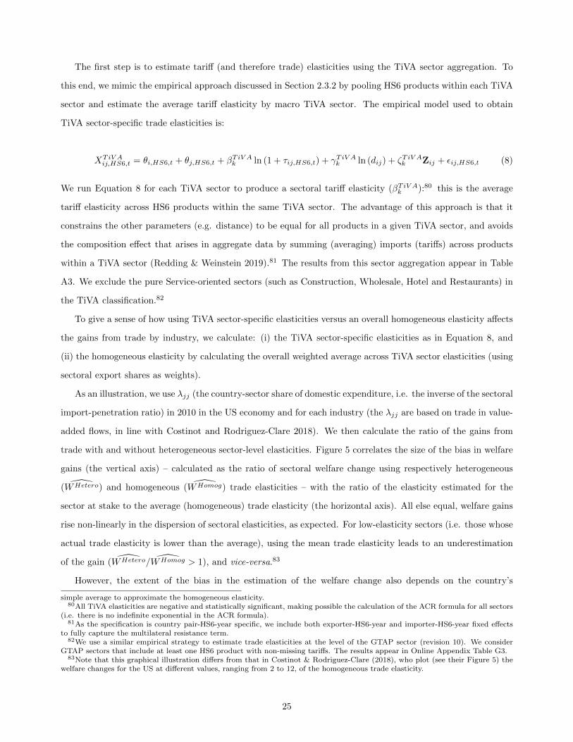
The first step is to estimate tariff (and therefore trade) elasticities using the TiVA sector aggregation. To
this end, we mimic the empirical approach discussed in Section 2.3.2 by pooling HS6 products within each TiVA
sector and estimate the average tariff elasticity by macro TiVA sector. The empirical model used to obtain
TiVA sector-specific trade elasticities is:
XTiV Aij,HS6,t = θi,HS6,t + θj,HS6,t + βTiV Ak ln (1 + τij,HS6,t) + γTiV Ak ln (dij) + ζTiV Ak Zij + εij,HS6,t (8)
We run Equation 8 for each TiVA sector to produce a sectoral tariff elasticity (βTiV Ak ):80 this is the average
tariff elasticity across HS6 products within the same TiVA sector. The advantage of this approach is that it
constrains the other parameters (e.g. distance) to be equal for all products in a given TiVA sector, and avoids
the composition effect that arises in aggregate data by summing (averaging) imports (tariffs) across products
within a TiVA sector (Redding & Weinstein 2019).81 The results from this sector aggregation appear in Table
A3. We exclude the pure Service-oriented sectors (such as Construction, Wholesale, Hotel and Restaurants) in
the TiVA classification.82
To give a sense of how using TiVA sector-specific elasticities versus an overall homogeneous elasticity affects
the gains from trade by industry, we calculate: (i) the TiVA sector-specific elasticities as in Equation 8, and
(ii) the homogeneous elasticity by calculating the overall weighted average across TiVA sector elasticities (using
sectoral export shares as weights).
As an illustration, we use λjj (the country-sector share of domestic expenditure, i.e. the inverse of the sectoral
import-penetration ratio) in 2010 in the US economy and for each industry (the λjj are based on trade in value-
added flows, in line with Costinot and Rodriguez-Clare 2018). We then calculate the ratio of the gains from
trade with and without heterogeneous sector-level elasticities. Figure 5 correlates the size of the bias in welfare
gains (the vertical axis) – calculated as the ratio of sectoral welfare change using respectively heterogeneous
(WHetero) and homogeneous (WHomog) trade elasticities – with the ratio of the elasticity estimated for the
sector at stake to the average (homogeneous) trade elasticity (the horizontal axis). All else equal, welfare gains
rise non-linearly in the dispersion of sectoral elasticities, as expected. For low-elasticity sectors (i.e. those whose
actual trade elasticity is lower than the average), using the mean trade elasticity leads to an underestimation
of the gain (WHetero/WHomog > 1), and vice-versa.83
However, the extent of the bias in the estimation of the welfare change also depends on the country’s
simple average to approximate the homogeneous elasticity.80All TiVA elasticities are negative and statistically significant, making possible the calculation of the ACR formula for all sectors
(i.e. there is no indefinite exponential in the ACR formula).81As the specification is country pair-HS6-year specific, we include both exporter-HS6-year and importer-HS6-year fixed effects
to fully capture the multilateral resistance term.82We use a similar empirical strategy to estimate trade elasticities at the level of the GTAP sector (revision 10). We consider
GTAP sectors that include at least one HS6 product with non-missing tariffs. The results appear in Online Appendix Table G3.83Note that this graphical illustration differs from that in Costinot & Rodriguez-Clare (2018), who plot (see their Figure 5) the
welfare changes for the US at different values, ranging from 2 to 12, of the homogeneous trade elasticity.
25
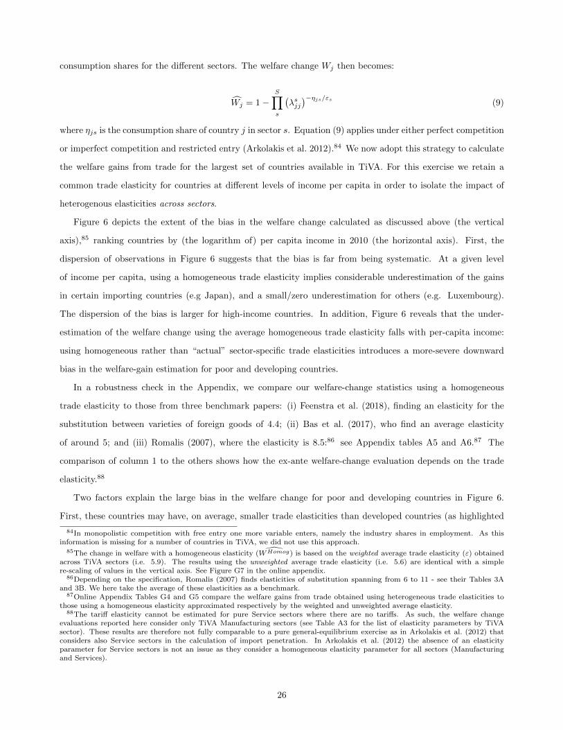
consumption shares for the different sectors. The welfare change Wj then becomes:
Wj = 1−S∏s
(λsjj)−ηjs/εs
(9)
where ηjs is the consumption share of country j in sector s. Equation (9) applies under either perfect competition
or imperfect competition and restricted entry (Arkolakis et al. 2012).84 We now adopt this strategy to calculate
the welfare gains from trade for the largest set of countries available in TiVA. For this exercise we retain a
common trade elasticity for countries at different levels of income per capita in order to isolate the impact of
heterogenous elasticities across sectors.
Figure 6 depicts the extent of the bias in the welfare change calculated as discussed above (the vertical
axis),85 ranking countries by (the logarithm of) per capita income in 2010 (the horizontal axis). First, the
dispersion of observations in Figure 6 suggests that the bias is far from being systematic. At a given level
of income per capita, using a homogeneous trade elasticity implies considerable underestimation of the gains
in certain importing countries (e.g Japan), and a small/zero underestimation for others (e.g. Luxembourg).
The dispersion of the bias is larger for high-income countries. In addition, Figure 6 reveals that the under-
estimation of the welfare change using the average homogeneous trade elasticity falls with per-capita income:
using homogeneous rather than “actual” sector-specific trade elasticities introduces a more-severe downward
bias in the welfare-gain estimation for poor and developing countries.
In a robustness check in the Appendix, we compare our welfare-change statistics using a homogeneous
trade elasticity to those from three benchmark papers: (i) Feenstra et al. (2018), finding an elasticity for the
substitution between varieties of foreign goods of 4.4; (ii) Bas et al. (2017), who find an average elasticity
of around 5; and (iii) Romalis (2007), where the elasticity is 8.5:86 see Appendix tables A5 and A6.87 The
comparison of column 1 to the others shows how the ex-ante welfare-change evaluation depends on the trade
elasticity.88
Two factors explain the large bias in the welfare change for poor and developing countries in Figure 6.
First, these countries may have, on average, smaller trade elasticities than developed countries (as highlighted
84In monopolistic competition with free entry one more variable enters, namely the industry shares in employment. As thisinformation is missing for a number of countries in TiVA, we did not use this approach.
85The change in welfare with a homogeneous elasticity ( WHomog) is based on the weighted average trade elasticity (ε) obtainedacross TiVA sectors (i.e. 5.9). The results using the unweighted average trade elasticity (i.e. 5.6) are identical with a simplere-scaling of values in the vertical axis. See Figure G7 in the online appendix.
86Depending on the specification, Romalis (2007) finds elasticities of substitution spanning from 6 to 11 - see their Tables 3Aand 3B. We here take the average of these elasticities as a benchmark.
87Online Appendix Tables G4 and G5 compare the welfare gains from trade obtained using heterogeneous trade elasticities tothose using a homogeneous elasticity approximated respectively by the weighted and unweighted average elasticity.
88The tariff elasticity cannot be estimated for pure Service sectors where there are no tariffs. As such, the welfare changeevaluations reported here consider only TiVA Manufacturing sectors (see Table A3 for the list of elasticity parameters by TiVAsector). These results are therefore not fully comparable to a pure general-equilibrium exercise as in Arkolakis et al. (2012) thatconsiders also Service sectors in the calculation of import penetration. In Arkolakis et al. (2012) the absence of an elasticityparameter for Service sectors is not an issue as they consider a homogeneous elasticity parameter for all sectors (Manufacturingand Services).
26
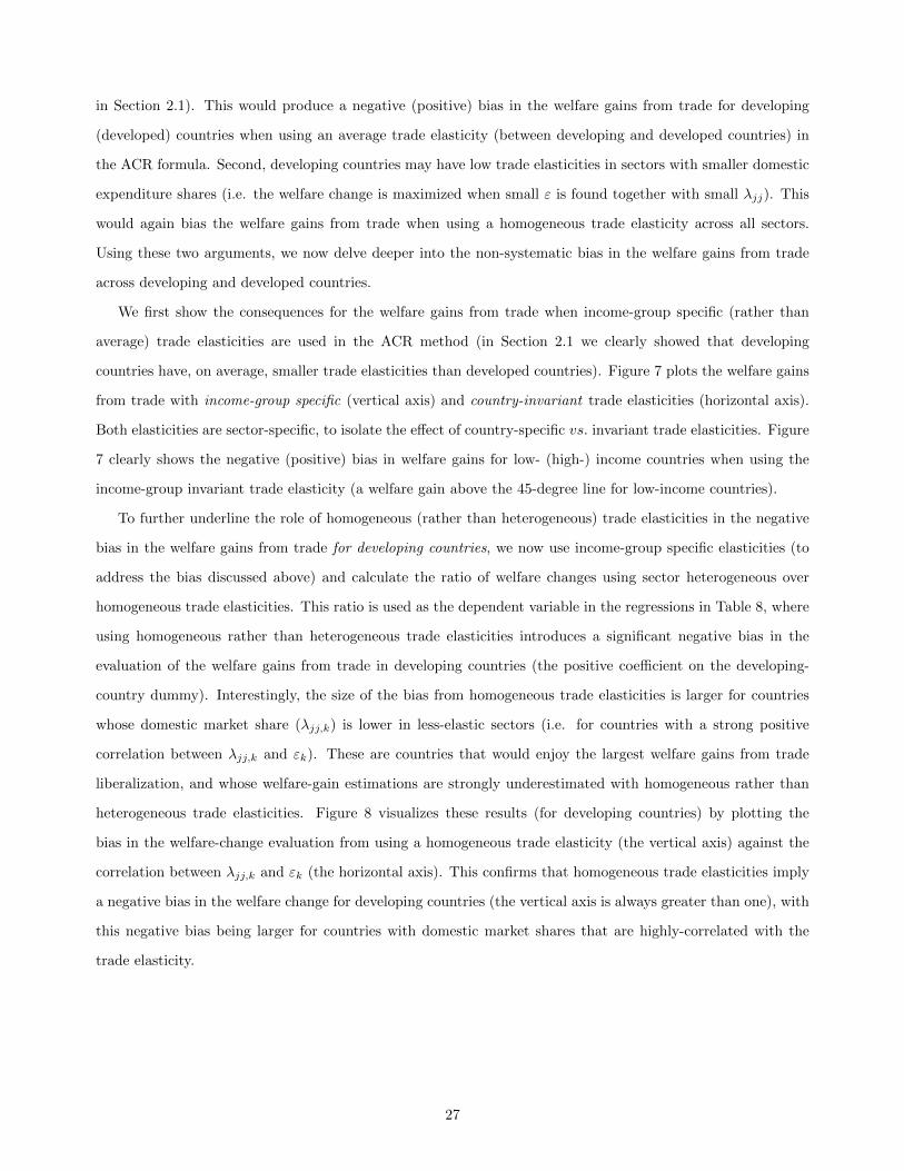
in Section 2.1). This would produce a negative (positive) bias in the welfare gains from trade for developing
(developed) countries when using an average trade elasticity (between developing and developed countries) in
the ACR formula. Second, developing countries may have low trade elasticities in sectors with smaller domestic
expenditure shares (i.e. the welfare change is maximized when small ε is found together with small λjj). This
would again bias the welfare gains from trade when using a homogeneous trade elasticity across all sectors.
Using these two arguments, we now delve deeper into the non-systematic bias in the welfare gains from trade
across developing and developed countries.
We first show the consequences for the welfare gains from trade when income-group specific (rather than
average) trade elasticities are used in the ACR method (in Section 2.1 we clearly showed that developing
countries have, on average, smaller trade elasticities than developed countries). Figure 7 plots the welfare gains
from trade with income-group specific (vertical axis) and country-invariant trade elasticities (horizontal axis).
Both elasticities are sector-specific, to isolate the effect of country-specific vs. invariant trade elasticities. Figure
7 clearly shows the negative (positive) bias in welfare gains for low- (high-) income countries when using the
income-group invariant trade elasticity (a welfare gain above the 45-degree line for low-income countries).
To further underline the role of homogeneous (rather than heterogeneous) trade elasticities in the negative
bias in the welfare gains from trade for developing countries, we now use income-group specific elasticities (to
address the bias discussed above) and calculate the ratio of welfare changes using sector heterogeneous over
homogeneous trade elasticities. This ratio is used as the dependent variable in the regressions in Table 8, where
using homogeneous rather than heterogeneous trade elasticities introduces a significant negative bias in the
evaluation of the welfare gains from trade in developing countries (the positive coefficient on the developing-
country dummy). Interestingly, the size of the bias from homogeneous trade elasticities is larger for countries
whose domestic market share (λjj,k) is lower in less-elastic sectors (i.e. for countries with a strong positive
correlation between λjj,k and εk). These are countries that would enjoy the largest welfare gains from trade
liberalization, and whose welfare-gain estimations are strongly underestimated with homogeneous rather than
heterogeneous trade elasticities. Figure 8 visualizes these results (for developing countries) by plotting the
bias in the welfare-change evaluation from using a homogeneous trade elasticity (the vertical axis) against the
correlation between λjj,k and εk (the horizontal axis). This confirms that homogeneous trade elasticities imply
a negative bias in the welfare change for developing countries (the vertical axis is always greater than one), with
this negative bias being larger for countries with domestic market shares that are highly-correlated with the
trade elasticity.
27
4 Conclusion
The first contribution of this paper is to provide estimates of trade elasticities at the product level, by exploiting
the variation over the 2001-2016 period in bilateral applied tariffs (a variable trade cost) for each product
category and the widest-possible set of importers, and so including countries at different level of development.
We combine two databases covering the universe of exporters, importers and products at the finest level of
disaggregation (the 6-digit level of the Harmonized System). Although we obtain an average trade elasticity
in line with that in the literature, we shed light on the wide range around the value that is generally used to
calibrate empirical exercises. This is the second contribution of our paper. We finally illustrate the impact of
heterogeneous trade elasticities on the estimation of the welfare gains from trade for countries at different levels
of development. This is carried out via a simple exercise in line with Arkolakis et al. (2012). We show that using
homogeneous trade elasticities produces a downward bias in the estimation of the welfare gains from trade for
developing countries, and in particular for those with considerable import penetration in less-elastic sectors.
28
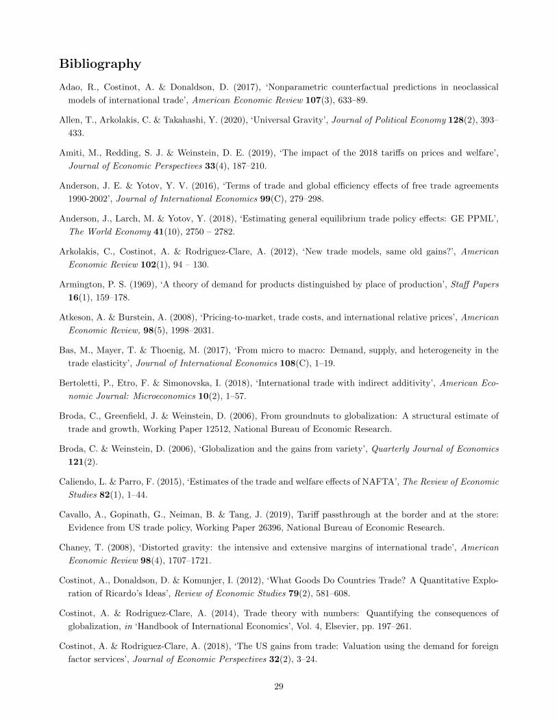
Bibliography
Adao, R., Costinot, A. & Donaldson, D. (2017), ‘Nonparametric counterfactual predictions in neoclassical
models of international trade’, American Economic Review 107(3), 633–89.
Allen, T., Arkolakis, C. & Takahashi, Y. (2020), ‘Universal Gravity’, Journal of Political Economy 128(2), 393–
433.
Amiti, M., Redding, S. J. & Weinstein, D. E. (2019), ‘The impact of the 2018 tariffs on prices and welfare’,
Journal of Economic Perspectives 33(4), 187–210.
Anderson, J. E. & Yotov, Y. V. (2016), ‘Terms of trade and global efficiency effects of free trade agreements
1990-2002’, Journal of International Economics 99(C), 279–298.
Anderson, J., Larch, M. & Yotov, Y. (2018), ‘Estimating general equilibrium trade policy effects: GE PPML’,
The World Economy 41(10), 2750 – 2782.
Arkolakis, C., Costinot, A. & Rodriguez-Clare, A. (2012), ‘New trade models, same old gains?’, American
Economic Review 102(1), 94 – 130.
Armington, P. S. (1969), ‘A theory of demand for products distinguished by place of production’, Staff Papers
16(1), 159–178.
Atkeson, A. & Burstein, A. (2008), ‘Pricing-to-market, trade costs, and international relative prices’, American
Economic Review, 98(5), 1998–2031.
Bas, M., Mayer, T. & Thoenig, M. (2017), ‘From micro to macro: Demand, supply, and heterogeneity in the
trade elasticity’, Journal of International Economics 108(C), 1–19.
Bertoletti, P., Etro, F. & Simonovska, I. (2018), ‘International trade with indirect additivity’, American Eco-
nomic Journal: Microeconomics 10(2), 1–57.
Broda, C., Greenfield, J. & Weinstein, D. (2006), From groundnuts to globalization: A structural estimate of
trade and growth, Working Paper 12512, National Bureau of Economic Research.
Broda, C. & Weinstein, D. (2006), ‘Globalization and the gains from variety’, Quarterly Journal of Economics
121(2).
Caliendo, L. & Parro, F. (2015), ‘Estimates of the trade and welfare effects of NAFTA’, The Review of Economic
Studies 82(1), 1–44.
Cavallo, A., Gopinath, G., Neiman, B. & Tang, J. (2019), Tariff passthrough at the border and at the store:
Evidence from US trade policy, Working Paper 26396, National Bureau of Economic Research.
Chaney, T. (2008), ‘Distorted gravity: the intensive and extensive margins of international trade’, American
Economic Review 98(4), 1707–1721.
Costinot, A., Donaldson, D. & Komunjer, I. (2012), ‘What Goods Do Countries Trade? A Quantitative Explo-
ration of Ricardo’s Ideas’, Review of Economic Studies 79(2), 581–608.
Costinot, A. & Rodriguez-Clare, A. (2014), Trade theory with numbers: Quantifying the consequences of
globalization, in ‘Handbook of International Economics’, Vol. 4, Elsevier, pp. 197–261.
Costinot, A. & Rodriguez-Clare, A. (2018), ‘The US gains from trade: Valuation using the demand for foreign
factor services’, Journal of Economic Perspectives 32(2), 3–24.
29
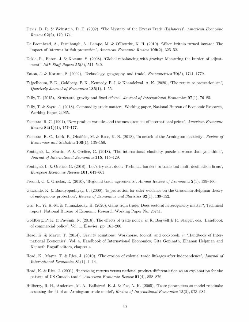
Davis, D. R. & Weinstein, D. E. (2002), ‘The Mystery of the Excess Trade (Balances)’, American Economic
Review 92(2), 170–174.
De Bromhead, A., Fernihough, A., Lampe, M. & O’Rourke, K. H. (2019), ‘When britain turned inward: The
impact of interwar british protection’, American Economic Review 109(2), 325–52.
Dekle, R., Eaton, J. & Kortum, S. (2008), ‘Global rebalancing with gravity: Measuring the burden of adjust-
ment’, IMF Staff Papers 55(3), 511–540.
Eaton, J. & Kortum, S. (2002), ‘Technology, geography, and trade’, Econometrica 70(5), 1741–1779.
Fajgelbaum, P. D., Goldberg, P. K., Kennedy, P. J. & Khandelwal, A. K. (2020), ‘The return to protectionism’,
Quarterly Journal of Economics 135(1), 1–55.
Fally, T. (2015), ‘Structural gravity and fixed effects’, Journal of International Economics 97(1), 76–85.
Fally, T. & Sayre, J. (2018), Commodity trade matters, Working paper, National Bureau of Economic Research,
Working Paper 24965.
Feenstra, R. C. (1994), ‘New product varieties and the measurement of international prices’, American Economic
Review 84(1)(1), 157–177.
Feenstra, R. C., Luck, P., Obstfeld, M. & Russ, K. N. (2018), ‘In search of the Armington elasticity’, Review of
Economics and Statistics 100(1), 135–150.
Fontagne, L., Martin, P. & Orefice, G. (2018), ‘The international elasticity puzzle is worse than you think’,
Journal of International Economics 115, 115–129.
Fontagne, L. & Orefice, G. (2018), ‘Let’s try next door: Technical barriers to trade and multi-destination firms’,
European Economic Review 101, 643–663.
Freund, C. & Ornelas, E. (2010), ‘Regional trade agreements’, Annual Review of Economics 2(1), 139–166.
Gawande, K. & Bandyopadhyay, U. (2000), ‘Is protection for sale? evidence on the Grossman-Helpman theory
of endogenous protection’, Review of Economics and Statistics 82(1), 139–152.
Giri, R., Yi, K.-M. & Yilmazkuday, H. (2020), Gains from trade: Does sectoral heterogeneity matter?, Technical
report, National Bureau of Economic Research Working Paper No. 26741.
Goldberg, P. K. & Pavcnik, N. (2016), The effects of trade policy, in K. Bagwell & R. Staiger, eds, ‘Handbook
of commercial policy’, Vol. 1, Elsevier, pp. 161–206.
Head, K. & Mayer, T. (2014), Gravity equations: Workhorse, toolkit, and cookbook, in ‘Handbook of Inter-
national Economics’, Vol. 4, Handbook of International Economics, Gita Gopinath, Elhanan Helpman and
Kenneth Rogoff editors, chapter 4.
Head, K., Mayer, T. & Ries, J. (2010), ‘The erosion of colonial trade linkages after independence’, Journal of
International Economics 81(1), 1–14.
Head, K. & Ries, J. (2001), ‘Increasing returns versus national product differentiation as an explanation for the
pattern of US-Canada trade’, American Economic Review 91(4), 858–876.
Hillberry, R. H., Anderson, M. A., Balistreri, E. J. & Fox, A. K. (2005), ‘Taste parameters as model residuals:
assessing the fit of an Armington trade model’, Review of International Economics 13(5), 973–984.
30
Hummels, D. (2007), ‘Transportation costs and international trade in the second era of globalization’, Journal
of Economic perspectives 21(3), 131–154.
Hummels, D. & Skiba, A. (2004), ‘Shipping the good apples out? An empirical confirmation of the Alchian-Allen
conjecture’, Journal of Political Economy 112(6), 1384–1402.
Imbs, J. & Mejean, I. (2015), ‘Elasticity Optimism’, American Economic Journal: Macroeconomics 3(7), 43–83.
Kee, H. L., Nicita, A. & Olarreaga, M. (2008), ‘Import demand elasticities and trade distortions’, Review of
Economics and Statistics 90(4), 666–682.
Kee, H. L., Nicita, A. & Olarreaga, M. (2009), ‘Estimating Trade Restrictiveness Indices’, Economic Journal
119(534), 172–199.
Machado, J. A. & Santos Silva, J. (2019), ‘Quantiles via moments’, Journal of Econometrics 213(1), 145–173.
Markusen, J. R. (2013), ‘Putting per-capita income back into trade theory’, Journal of International Economics
90(2), 255–265.
Martin, P., Mayer, T. & Thoenig, M. (2008), ‘Make trade not war?’, Review of Economic Studies 75(3), 865–900.
Melitz, M. J. & Redding, S. J. (2015), ‘New trade models, new welfare implications’, American Economic Review
105(3), 1105–46.
Mrazova, M. & Neary, P. (2017), ‘Not so demanding: Demand structure and firm behavior’, American Economic
Review 107(12), 3835–74.
Mrazova, M., Neary, P. & Carrere, C. (2020), ‘Gravity without apologies: the science of elasticities, distance,
and trade’, Economic Journal forthcoming.
Ossa, R. (2014), ‘Trade wars and trade talks with data’, American Economic Review 104(12), 4104–46.
Ossa, R. (2015), ‘Why trade matters after all’, Journal of International Economics 97(2), 266–277.
Redding, S. J. & Weinstein, D. E. (2019), Aggregation and the gravity equation, in ‘AEA Papers and Proceed-
ings’, Vol. 109, pp. 450–55.
Romalis, J. (2007), ‘NAFTA’s and CUSFTA’s impact on international trade’, Review of Economics and Statistics
89(3), 416–435.
Santos-Silva, J. M. C. & Tenreyro, S. (2006), ‘The Log of Gravity’, The Review of Economics and Statistics
88(4), 641–658.
Sequeira, S. (2016), ‘Corruption, Trade Costs, and Gains from Tariff Liberalization: Evidence from Southern
Africa’, American Economic Review 106(10), 3029–3063.
Shapiro, J. S. (2016), ‘Trade costs, CO2, and the environment’, American Economic Journal: Economic Policy
8(4), 220–54.
Simonovska, I. & Waugh, M. E. (2014a), ‘The elasticity of trade: Estimates and evidence’, Journal of Interna-
tional Economics 92(1), 34 – 50.
Soderbery, A. (2018), ‘Trade elasticities, heterogeneity, and optimal tariffs’, Journal of International Economics
114, 44–62.
Spearot, A. C. (2013), ‘Variable demand elasticities and tariff liberalization’, Journal of International Economics
89(1), 26–41.
31
Tables and Figures
Table 1: Tests for pre-existing trends.
Dep Var: Average import growth before the first change in tariffAvg tariff growth after first change in tariff 0.134 -0.031 0.073 0.079 0.431
(0.252) (0.265) (0.134) (0.137) (0.384)Exporter FE No No Yes No NoImporter FE No No Yes No NoProduct FE No Yes Yes Yes NoExporter x Importer FE No No No Yes NoExporter x Product FE No No No No YesImporter x Product FE No No No No YesObservations 1,130,580 1,130,569 1,130,564 1,129,206 1,005,049R-squared 0.000 0.013 0.043 0.067 0.338
Notes: This table shows the pre-trend test for import demand. The dependent variable is the average growth rate of imports(i.e. ln (Import)ijk,t - ln (Import)ijk,t−1) before the first change in the tariff imposed by importer i on variety jk. Theexplanatory variable is the average growth rate in tariffs after the first change in tariff (ln(1 + τijk,t) - ln(1 + τijk,t−1)).Source: Authors’ calculations.
Table 2: The share of non-missing importer-exporter-HS6 cells with zero vs. non-zero tariffs (divided into MFN,preferential and non-WTO).
Share of importer-exporter-product cells with:
Zero Applied Non-zero Applied TariffsTariffs Preferential MFN Non-WTO
2001 18.7 67.4 13.0 1.02004 31.0 65.6 3.3 0.12007 35.7 60.8 3.2 0.42010 37.8 58.1 3.6 0.52013 39.5 55.9 4.1 0.52016 40.1 56.3 3.6 0.1
Notes: Columns 2 and 3-5 list the share of non-missing importer-exporter-HS6 combinations with respectively zero and non-zero tariffs in force.Columns 3-5 show the share of preferential, MFN and non-WTO non-zerotariffs. Source: MAcMap-HS6, authors’ calculations.
32
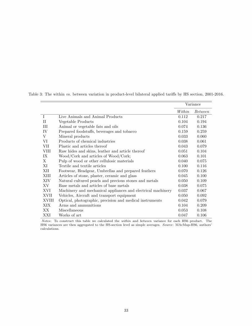
Table 3: The within vs. between variation in product-level bilateral applied tariffs by HS section, 2001-2016.
Variance
Within BetweenI Live Animals and Animal Products 0.112 0.217II Vegetable Products 0.104 0.194III Animal or vegetable fats and oils 0.074 0.136IV Prepared foodstuffs, beverages and tobacco 0.159 0.259V Mineral products 0.033 0.060VI Products of chemical industries 0.038 0.061VII Plastic and articles thereof 0.043 0.079VIII Raw hides and skins, leather and article thereof 0.051 0.104IX Wood/Cork and articles of Wood/Cork; 0.063 0.101X Pulp of wood or other cellulosic materials 0.040 0.075XI Textile and textile articles 0.100 0.116XII Footwear, Headgear, Umbrellas and prepared feathers 0.070 0.126XIII Articles of stone, plaster, ceramic and glass 0.045 0.100XIV Natural cultured pearls and precious stones and metals 0.050 0.109XV Base metals and articles of base metals 0.038 0.075XVI Machinery and mechanical appliances and electrical machinery 0.037 0.067XVII Vehicles, Aircraft and transport equipment 0.050 0.092XVIII Optical, photographic, precision and medical instruments 0.042 0.079XIX Arms and ammunitions 0.104 0.209XX Miscellaneous 0.053 0.108XXI Works of art 0.047 0.106
Notes: To construct this table we calculated the within and between variance for each HS6 product. TheHS6 variances are then aggregated to the HS-section level as simple averages. Source: MAcMap-HS6, authors’calculations.
33
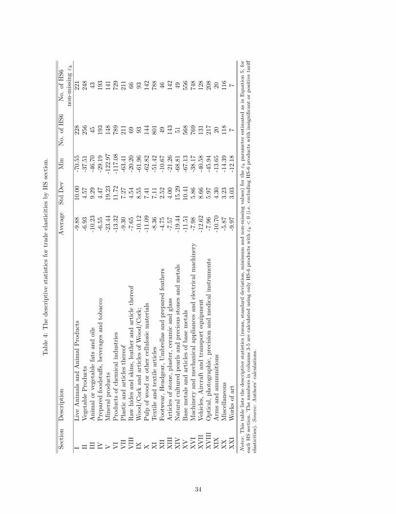
Tab
le4:
Th
ed
escr
ipti
vest
ati
stic
sfo
rtr
ad
eel
ast
icit
ies
by
HS
sect
ion
.
Sec
tion
Des
crip
tion
Aver
age
Std
Dev
Min
No.
of
HS
6N
o.
of
HS
6n
on
-mis
sin
gε k
IL
ive
An
imal
san
dA
nim
alP
rod
uct
s-9
.88
10.0
0-7
0.5
5228
221
IIV
eget
able
Pro
du
cts
-6.9
34.5
7-3
7.5
1256
248
III
An
imal
orve
geta
ble
fats
and
oils
-10.2
39.2
9-4
6.7
045
43
IVP
repar
edfo
od
stu
ffs,
bev
erag
esan
dto
bacc
o-6
.55
4.4
7-2
9.1
9193
193
VM
iner
alp
rod
uct
s-2
3.4
419.2
3-1
22.
97
148
141
VI
Pro
du
cts
ofch
emic
alin
du
stri
es-1
3.3
211.7
2-1
17.0
8789
729
VII
Pla
stic
and
arti
cles
ther
eof
-9.3
07.2
7-6
3.4
1211
211
VII
IR
awh
ides
and
skin
s,le
ath
eran
dart
icle
ther
eof
-7.6
54.5
4-2
0.2
069
66
IXW
ood
/Cor
kan
dar
ticl
esof
Wood
/C
ork
;-1
0.1
28.5
5-6
1.9
693
93
XP
ulp
ofw
ood
orot
her
cell
ulo
sic
mate
rials
-11.0
97.4
1-6
2.8
2144
142
XI
Tex
tile
and
texti
lear
ticl
es-8
.36
7.1
1-5
1.4
2801
788
XII
Foot
wea
r,H
ead
gear
,U
mb
rell
asan
dp
rep
are
dfe
ath
ers
-4.7
52.5
2-1
0.6
749
46
XII
IA
rtic
les
ofst
one,
pla
ster
,ce
ram
ican
dgla
ss-7
.57
4.0
0-2
1.2
6143
142
XIV
Nat
ura
lcu
ltu
red
pea
rls
and
pre
ciou
sst
on
esan
dm
etals
-19.4
415.2
9-6
8.8
151
49
XV
Bas
em
etal
san
dar
ticl
esof
bas
em
etals
-11.5
110.4
1-6
7.1
3568
556
XV
IM
ach
iner
yan
dm
ech
anic
alap
pli
an
ces
an
del
ectr
ical
mach
iner
y-7
.98
5.8
6-3
8.1
7769
748
XV
IIV
ehic
les,
Air
craf
tan
dtr
ansp
ort
equ
ipm
ent
-12.6
28.6
6-4
0.5
8131
128
XV
III
Op
tica
l,p
hot
ogra
ph
ic,
pre
cisi
onan
dm
edic
al
inst
rum
ents
-7.9
65.9
7-4
5.9
4217
208
XIX
Arm
san
dam
mu
nit
ion
s-1
0.7
04.3
0-1
3.6
520
20
XX
Mis
cell
aneo
us
-5.8
73.2
3-1
4.3
9118
116
XX
IW
orks
ofar
t-9
.97
3.0
3-1
2.1
87
7
Notes:
Th
ista
ble
list
sth
ed
escr
ipti
ve
stati
stic
s(m
ean
,st
an
dard
dev
iati
on
,m
inim
um
an
dn
on
-mis
sin
gvalu
es)
for
theε k
para
met
eres
tim
ate
das
inE
qu
ati
on
5,
for
each
HS
sect
ion
.T
he
nu
mb
ers
inco
lum
ns
3-5
are
calc
ula
ted
usi
ng
on
lyH
S-6
pro
du
cts
wit
hε k<
0(i
.e.
excl
ud
ing
HS
-6p
rod
uct
sw
ith
insi
gn
ifica
nt
or
posi
tive
tari
ffel
ast
icit
ies)
.Source:
Au
thors
’ca
lcu
lati
on
s.
34
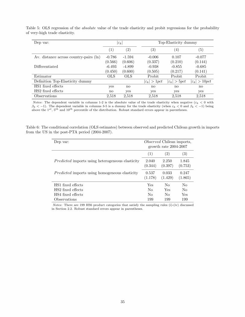
Table 5: OLS regression of the absolute value of the trade elasticity and probit regressions for the probabilityof very-high trade elasticity.
Dep var: |εk| Top-Elasticity dummy
(1) (2) (3) (4) (5)
Av. distance across country-pairs (ln) -0.786 -1.594 -0.006 0.107 -0.077(0.566) (0.606) (0.337) (0.210) (0.144)
Differentiated -6.493 -4.899 -0.938 -0.855 -0.685(0.450) (0.600) (0.505) (0.217) (0.141)
Estimator OLS OLS Probit Probit ProbitDefinition Top-Elasticity dummy |εk| > 1pct |εk| > 5pct |εk| > 10pctHS1 fixed effects yes no no no noHS2 fixed effects no yes yes yes yesObservations 2,518 2,518 2,518 2,518 2,518
Notes: The dependent variable in columns 1-2 is the absolute value of the trade elasticity when negative (εk < 0 withβk < −1). The dependent variable in columns 3-5 is a dummy for the trade elasticity (when εk < 0 and βk < −1) beingabove the 1st, 5th and 10th percentile of the distribution. Robust standard errors appear in parentheses.
Table 6: The conditional correlation (OLS estimates) between observed and predicted Chilean growth in importsfrom the US in the post-PTA period (2004-2007).
Dep var: Observed Chilean imports,growth rate 2004-2007
(1) (2) (3)
Predicted imports using heterogeneous elasticity 2.040 2.250 1.845(0.344) (0.397) (0.753)
Predicted imports using homogeneous elasticity 0.537 0.033 0.247(1.178) (1.429) (1.865)
HS1 fixed effects Yes No NoHS2 fixed effects No Yes NoHS4 fixed effects No No YesObservations 199 199 199
Notes: There are 199 HS6 product categories that satisfy the sampling rules (i)-(iv) discussedin Section 2.2. Robust standard errors appear in parentheses.
35
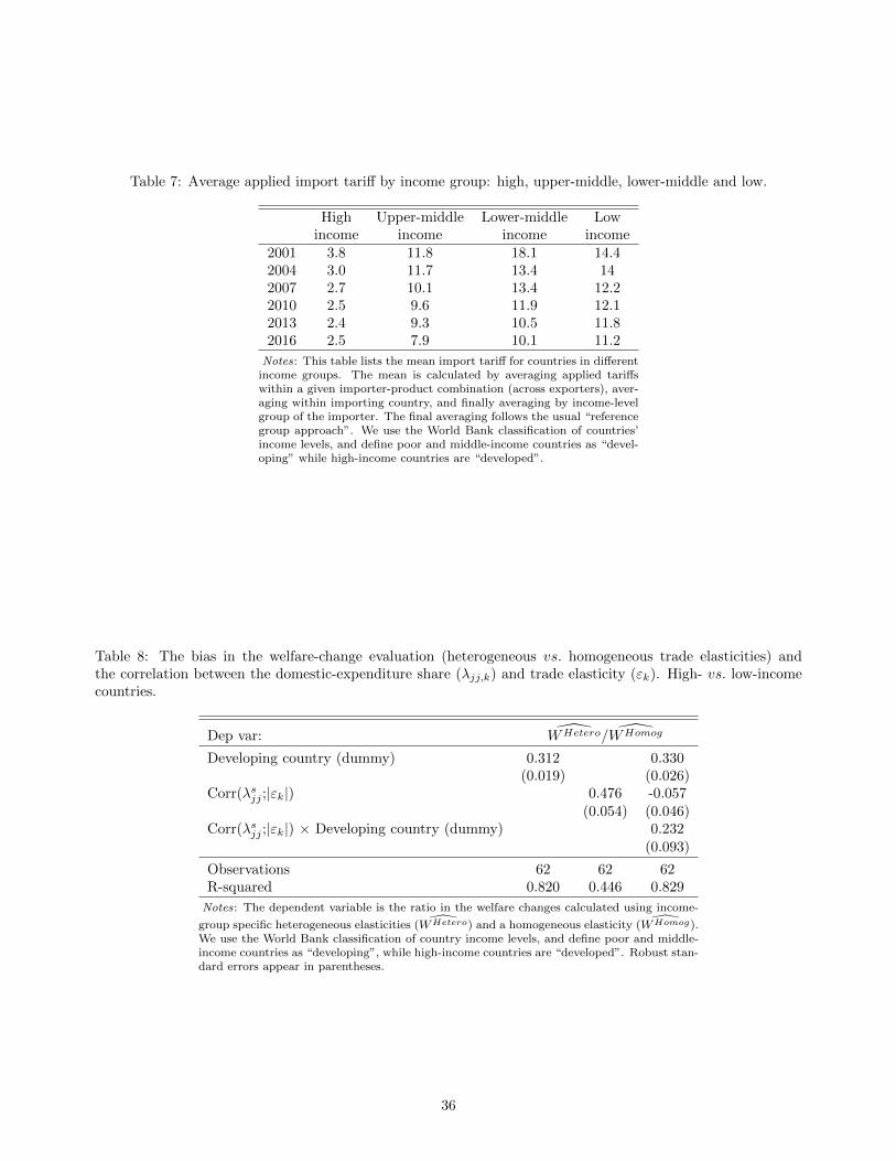
Table 7: Average applied import tariff by income group: high, upper-middle, lower-middle and low.
High Upper-middle Lower-middle Lowincome income income income
2001 3.8 11.8 18.1 14.42004 3.0 11.7 13.4 142007 2.7 10.1 13.4 12.22010 2.5 9.6 11.9 12.12013 2.4 9.3 10.5 11.82016 2.5 7.9 10.1 11.2
Notes: This table lists the mean import tariff for countries in differentincome groups. The mean is calculated by averaging applied tariffswithin a given importer-product combination (across exporters), aver-aging within importing country, and finally averaging by income-levelgroup of the importer. The final averaging follows the usual “referencegroup approach”. We use the World Bank classification of countries’income levels, and define poor and middle-income countries as “devel-oping” while high-income countries are “developed”.
Table 8: The bias in the welfare-change evaluation (heterogeneous vs. homogeneous trade elasticities) andthe correlation between the domestic-expenditure share (λjj,k) and trade elasticity (εk). High- vs. low-incomecountries.
Dep var: WHetero/WHomog
Developing country (dummy) 0.312 0.330(0.019) (0.026)
Corr(λsjj ;|εk|) 0.476 -0.057(0.054) (0.046)
Corr(λsjj ;|εk|) × Developing country (dummy) 0.232(0.093)
Observations 62 62 62R-squared 0.820 0.446 0.829
Notes: The dependent variable is the ratio in the welfare changes calculated using income-
group specific heterogeneous elasticities ( WHetero) and a homogeneous elasticity ( WHomog).We use the World Bank classification of country income levels, and define poor and middle-income countries as “developing”, while high-income countries are “developed”. Robust stan-dard errors appear in parentheses.
36
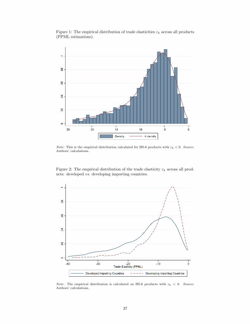
Figure 1: The empirical distribution of trade elasticities εk across all products(PPML estimations).
Note: This is the empirical distribution calculated for HS-6 products with εk < 0. Source:Authors’ calculations.
Figure 2: The empirical distribution of the trade elasticity εk across all prod-ucts: developed vs. developing importing countries.
Note: The empirical distribution is calculated on HS-6 products with εk < 0. Source:Authors’ calculations.
37
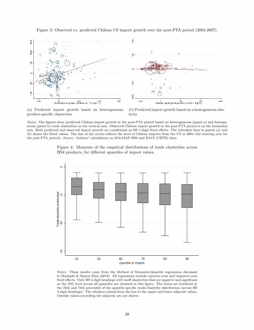
Figure 3: Observed vs. predicted Chilean US import growth over the post-PTA period (2004-2007).
(a) Predicted import growth based on heterogeneousproduct-specific elasticities
(b) Predicted import growth based on a homogeneous elas-ticity
Notes: The figures show predicted Chilean import growth in the post-PTA period based on heterogeneous (panel a) and homoge-neous (panel b) trade elasticities on the vertical axis. Observed Chilean import growth in the post-PTA period is on the horizontalaxis. Both predicted and observed import growth are conditional on HS 1-digit fixed effects. The unbroken lines in panels (a) and(b) shows the fitted values. The size of the circles reflects the level of Chilean imports from the US in 2004 (the starting year forthe post-PTA period). Source: Authors’ calculations on MAcMAP-HS6 and BACI (CEPII) data.
Figure 4: Moments of the empirical distributions of trade elasticities acrossHS4 products, for different quantiles of import values.
Notes: These results come from the Method of Moments-Quantile regressions discussedin Machado & Santos Silva (2019). All regressions include exporter-year and importer-yearfixed effects. Only HS 4-digit headings with tariff elasticities that are negative and significantat the 10% level across all quantiles are retained in this figure. The boxes are bordered atthe 25th and 75th percentile of the quantile-specific trade-elasticity distribution (across HS4-digit headings). The whiskers extend from the box to the upper and lower adjacent values.Outside values exceeding the adjacent are not shown.
38
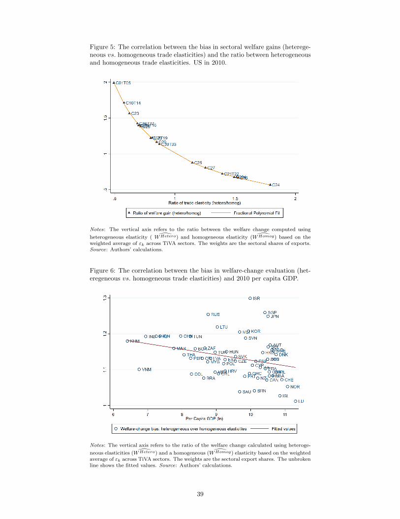
Figure 5: The correlation between the bias in sectoral welfare gains (heterege-neous vs. homogeneous trade elasticities) and the ratio between heterogeneousand homogeneous trade elasticities. US in 2010.
Notes: The vertical axis refers to the ratio between the welfare change computed using
heterogeneous elasticity ( WHetero) and homogeneous elasticity ( WHomog) based on theweighted average of εk across TiVA sectors. The weights are the sectoral shares of exports.Source: Authors’ calculations.
Figure 6: The correlation between the bias in welfare-change evaluation (het-eregeneous vs. homogeneous trade elasticities) and 2010 per capita GDP.
Notes: The vertical axis refers to the ratio of the welfare change calculated using heteroge-
neous elasticities ( WHetero) and a homogeneous ( WHomog) elasticity based on the weightedaverage of εk across TiVA sectors. The weights are the sectoral export shares. The unbrokenline shows the fitted values. Source: Authors’ calculations.
39
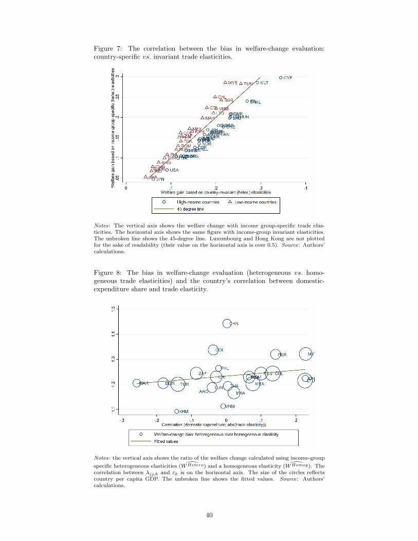
Figure 7: The correlation between the bias in welfare-change evaluation:country-specific vs. invariant trade elasticities.
Notes: The vertical axis shows the welfare change with income group-specific trade elas-ticities. The horizontal axis shows the same figure with income-group invariant elasticities.The unbroken line shows the 45-degree line. Luxembourg and Hong Kong are not plottedfor the sake of readability (their value on the horizontal axis is over 0.5). Source: Authors’calculations.
Figure 8: The bias in welfare-change evaluation (heterogeneous vs. homo-geneous trade elasticities) and the country’s correlation between domestic-expenditure share and trade elasticity.
Notes: the vertical axis shows the ratio of the welfare change calculated using income-group
specific heterogeneous elasticities ( WHetero) and a homogeneous elasticity ( WHomog). Thecorrelation between λjj,k and εk is on the horizontal axis. The size of the circles reflectscountry per capita GDP. The unbroken line shows the fitted values. Source: Authors’calculations.
40
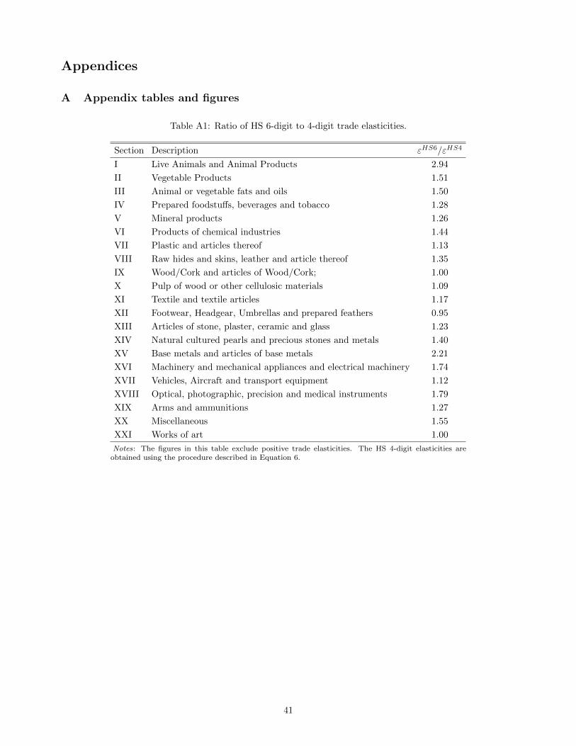
Appendices
A Appendix tables and figures
Table A1: Ratio of HS 6-digit to 4-digit trade elasticities.
Section Description εHS6/εHS4
I Live Animals and Animal Products 2.94
II Vegetable Products 1.51
III Animal or vegetable fats and oils 1.50
IV Prepared foodstuffs, beverages and tobacco 1.28
V Mineral products 1.26
VI Products of chemical industries 1.44
VII Plastic and articles thereof 1.13
VIII Raw hides and skins, leather and article thereof 1.35
IX Wood/Cork and articles of Wood/Cork; 1.00
X Pulp of wood or other cellulosic materials 1.09
XI Textile and textile articles 1.17
XII Footwear, Headgear, Umbrellas and prepared feathers 0.95
XIII Articles of stone, plaster, ceramic and glass 1.23
XIV Natural cultured pearls and precious stones and metals 1.40
XV Base metals and articles of base metals 2.21
XVI Machinery and mechanical appliances and electrical machinery 1.74
XVII Vehicles, Aircraft and transport equipment 1.12
XVIII Optical, photographic, precision and medical instruments 1.79
XIX Arms and ammunitions 1.27
XX Miscellaneous 1.55
XXI Works of art 1.00
Notes: The figures in this table exclude positive trade elasticities. The HS 4-digit elasticities areobtained using the procedure described in Equation 6.
41
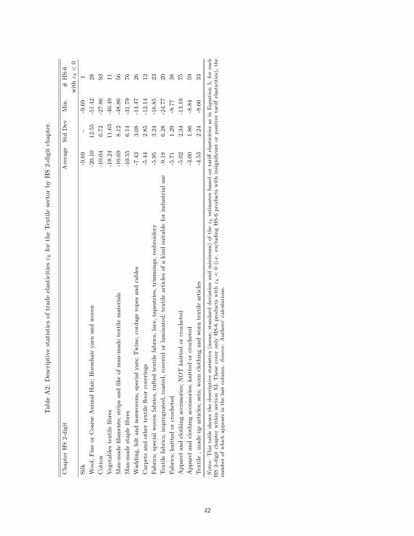
Tab
leA
2:D
escr
ipti
ve
stati
stic
sof
trad
eel
ast
icit
iesε k
for
the
Tex
tile
sect
or
by
HS
2-d
igit
chap
ter.
Chapte
rH
S2-d
igit
Aver
age
Std
Dev
Min
#H
S-6
wit
hε k
<0
Silk
-9.6
9-
-9.6
91
Wool,
Fin
eor
Coars
eA
nim
al
Hair
;H
ors
ehair
yarn
and
wov
en-2
0.1
012.5
5-5
1.4
228
Cott
on
-10.0
46.7
2-2
7.8
693
Veg
etable
ste
xti
lefibre
s-1
8.2
411.6
3-4
0.4
911
Man-m
ade
fila
men
ts;
stri
ps
and
like
of
man-m
ade
texti
lem
ate
rials
-10.6
98.1
2-4
8.8
656
Man-m
ade
staple
fibre
s-1
0.5
56.1
4-3
1.7
976
Waddin
g,
felt
and
nonw
oven
s,sp
ecia
lyars
;T
win
e,co
rdage
rop
esand
cable
s-7
.43
3.0
8-1
4.4
726
Carp
ets
and
oth
erte
xti
lefloor
cover
ings
-5.4
42.8
5-1
2.1
412
Fabri
cs;
spec
ial
wov
enfa
bri
cs,
tuft
edte
xti
lefa
bri
cs,
lace
,ta
pes
trie
s,tr
imm
ings,
embro
ider
y-5
.95
3.2
4-1
6.8
523
Tex
tile
fabri
cs;
impre
gnate
d,
coate
d,
cover
edor
lam
inate
d;
texti
leart
icle
sof
akin
dsu
itable
for
indust
rial
use
-9.1
86.2
8-2
4.7
720
Fabri
cs;
knit
ted
or
croch
eted
-5.7
11.2
9-8
.77
38
Appare
land
cloth
ing
acc
esso
ries
;N
OT
knit
ted
or
croch
eted
-5.0
22.3
4-1
3.1
875
Appare
land
cloth
ing
acc
esso
ries
;knit
ted
or
croch
eted
-3.0
01.8
6-8
.84
59
Tex
tile
,m
ade
up
art
icle
s;se
ts;
worn
cloth
ing
and
worn
texti
leart
icle
s-4
.53
2.2
4-8
.66
33
Notes:
Th
ista
ble
show
sth
ed
escr
ipti
ve
stati
stic
s(m
ean
,st
an
dard
dev
iati
on
an
dm
inim
um
)of
theε k
esti
mate
sb
ase
don
tari
ffel
ast
icit
ies
as
inE
qu
ati
on
5,
for
each
HS
2-d
igit
chap
ter
wit
hin
sect
ion
XI.
Th
ese
cover
on
lyH
S-6
pro
du
cts
wit
hε k
<0
(i.e
.ex
clu
din
gH
S-6
pro
du
cts
wit
hin
sign
ifica
nt
or
posi
tive
tari
ffel
ast
icit
ies)
,th
enu
mb
erof
wh
ich
ap
pea
rsin
the
last
colu
mn
.Source:
Au
thors
’ca
lcu
lati
on
s.
42
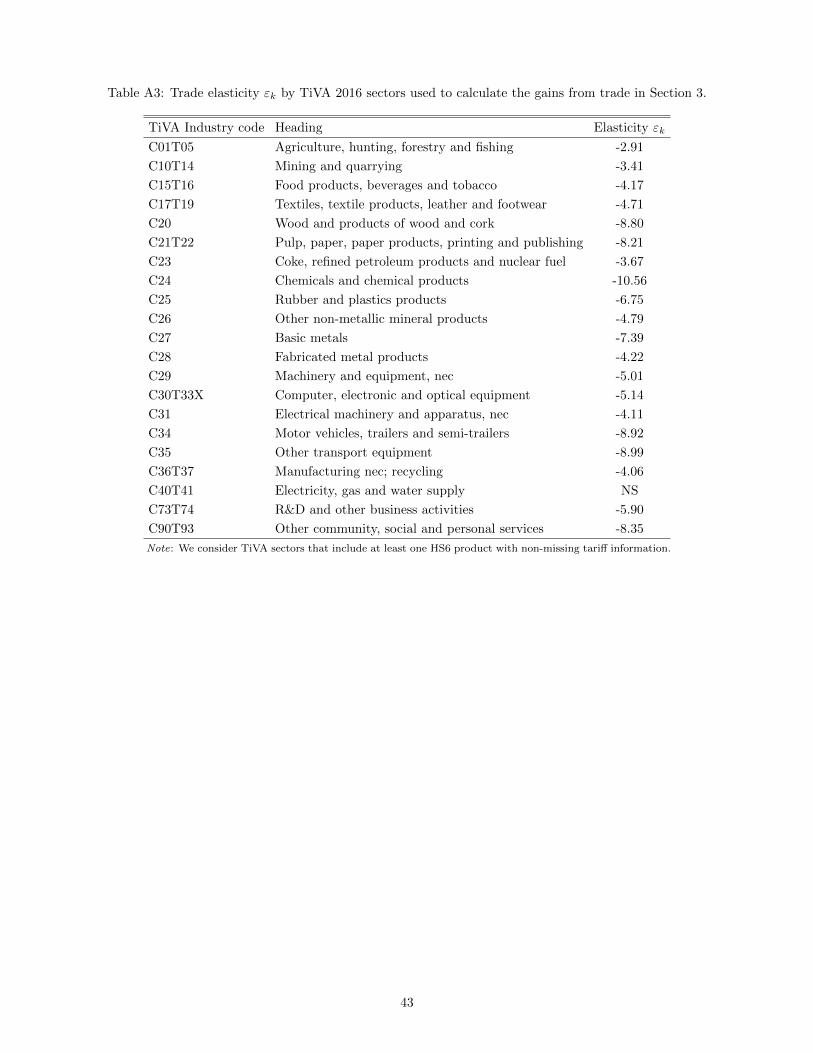
Table A3: Trade elasticity εk by TiVA 2016 sectors used to calculate the gains from trade in Section 3.
TiVA Industry code Heading Elasticity εk
C01T05 Agriculture, hunting, forestry and fishing -2.91
C10T14 Mining and quarrying -3.41
C15T16 Food products, beverages and tobacco -4.17
C17T19 Textiles, textile products, leather and footwear -4.71
C20 Wood and products of wood and cork -8.80
C21T22 Pulp, paper, paper products, printing and publishing -8.21
C23 Coke, refined petroleum products and nuclear fuel -3.67
C24 Chemicals and chemical products -10.56
C25 Rubber and plastics products -6.75
C26 Other non-metallic mineral products -4.79
C27 Basic metals -7.39
C28 Fabricated metal products -4.22
C29 Machinery and equipment, nec -5.01
C30T33X Computer, electronic and optical equipment -5.14
C31 Electrical machinery and apparatus, nec -4.11
C34 Motor vehicles, trailers and semi-trailers -8.92
C35 Other transport equipment -8.99
C36T37 Manufacturing nec; recycling -4.06
C40T41 Electricity, gas and water supply NS
C73T74 R&D and other business activities -5.90
C90T93 Other community, social and personal services -8.35
Note: We consider TiVA sectors that include at least one HS6 product with non-missing tariff information.
43
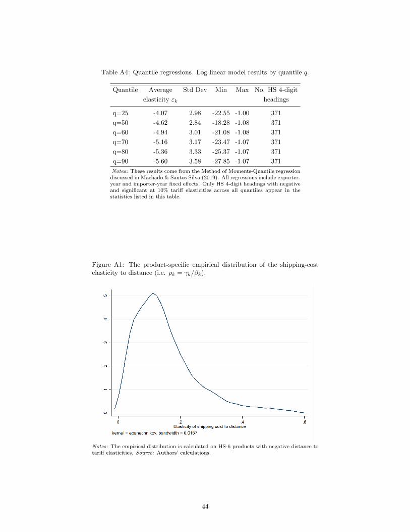
Table A4: Quantile regressions. Log-linear model results by quantile q.
Quantile Average Std Dev Min Max No. HS 4-digit
elasticity εk headings
q=25 -4.07 2.98 -22.55 -1.00 371
q=50 -4.62 2.84 -18.28 -1.08 371
q=60 -4.94 3.01 -21.08 -1.08 371
q=70 -5.16 3.17 -23.47 -1.07 371
q=80 -5.36 3.33 -25.37 -1.07 371
q=90 -5.60 3.58 -27.85 -1.07 371
Notes: These results come from the Method of Moments-Quantile regressiondiscussed in Machado & Santos Silva (2019). All regressions include exporter-year and importer-year fixed effects. Only HS 4-digit headings with negativeand significant at 10% tariff elasticities across all quantiles appear in thestatistics listed in this table.
Figure A1: The product-specific empirical distribution of the shipping-costelasticity to distance (i.e. ρk = γk/βk).
Notes: The empirical distribution is calculated on HS-6 products with negative distance totariff elasticities. Source: Authors’ calculations.
44
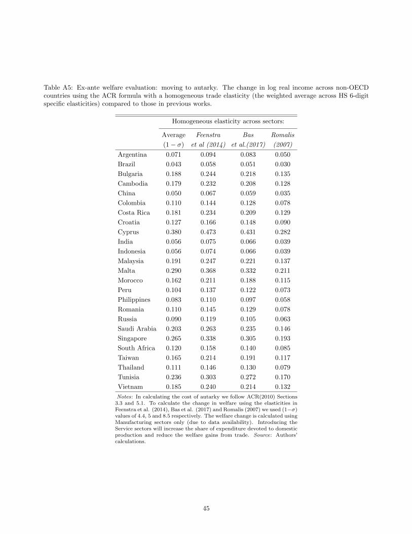
Table A5: Ex-ante welfare evaluation: moving to autarky. The change in log real income across non-OECDcountries using the ACR formula with a homogeneous trade elasticity (the weighted average across HS 6-digitspecific elasticities) compared to those in previous works.
Homogeneous elasticity across sectors:
Average Feenstra Bas Romalis
(1− σ) et al (2014) et al.(2017) (2007)
Argentina 0.071 0.094 0.083 0.050
Brazil 0.043 0.058 0.051 0.030
Bulgaria 0.188 0.244 0.218 0.135
Cambodia 0.179 0.232 0.208 0.128
China 0.050 0.067 0.059 0.035
Colombia 0.110 0.144 0.128 0.078
Costa Rica 0.181 0.234 0.209 0.129
Croatia 0.127 0.166 0.148 0.090
Cyprus 0.380 0.473 0.431 0.282
India 0.056 0.075 0.066 0.039
Indonesia 0.056 0.074 0.066 0.039
Malaysia 0.191 0.247 0.221 0.137
Malta 0.290 0.368 0.332 0.211
Morocco 0.162 0.211 0.188 0.115
Peru 0.104 0.137 0.122 0.073
Philippines 0.083 0.110 0.097 0.058
Romania 0.110 0.145 0.129 0.078
Russia 0.090 0.119 0.105 0.063
Saudi Arabia 0.203 0.263 0.235 0.146
Singapore 0.265 0.338 0.305 0.193
South Africa 0.120 0.158 0.140 0.085
Taiwan 0.165 0.214 0.191 0.117
Thailand 0.111 0.146 0.130 0.079
Tunisia 0.236 0.303 0.272 0.170
Vietnam 0.185 0.240 0.214 0.132
Notes: In calculating the cost of autarky we follow ACR(2010) Sections3.3 and 5.1. To calculate the change in welfare using the elasticities inFeenstra et al. (2014), Bas et al. (2017) and Romalis (2007) we used (1−σ)values of 4.4, 5 and 8.5 respectively. The welfare change is calculated usingManufacturing sectors only (due to data availability). Introducing theService sectors will increase the share of expenditure devoted to domesticproduction and reduce the welfare gains from trade. Source: Authors’calculations.
45
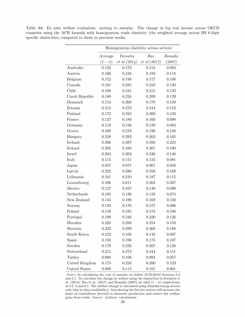
Table A6: Ex ante welfare evaluation: moving to autarky. The change in log real income across OECDcountries using the ACR formula with homogeneous trade elasticity (the weighted average across HS 6-digitspecific elasticities) compared to those in previous works.
Homogeneous elasticity across sectors:
Average Feenstra Bas Romalis
(1− σ) et al (2014) et al.(2017) (2007)
Australia 0.132 0.173 0.154 0.094
Austria 0.166 0.216 0.193 0.118
Belgium 0.152 0.198 0.177 0.108
Canada 0.181 0.235 0.210 0.130
Chile 0.186 0.241 0.215 0.133
Czech Republic 0.180 0.234 0.209 0.129
Denmark 0.154 0.200 0.179 0.109
Estonia 0.212 0.273 0.244 0.152
Finland 0.172 0.224 0.200 0.123
France 0.137 0.180 0.160 0.098
Germany 0.119 0.156 0.139 0.084
Greece 0.169 0.219 0.196 0.120
Hungary 0.228 0.293 0.263 0.165
Iceland 0.306 0.387 0.350 0.224
Ireland 0.262 0.334 0.301 0.190
Israel 0.204 0.263 0.236 0.146
Italy 0.115 0.151 0.134 0.081
Japan 0.057 0.075 0.067 0.040
Latvia 0.222 0.286 0.256 0.160
Lithuania 0.161 0.210 0.187 0.115
Luxembourg 0.506 0.611 0.564 0.387
Mexico 0.127 0.167 0.148 0.090
Netherlands 0.105 0.139 0.123 0.074
New Zealand 0.145 0.190 0.169 0.103
Norway 0.135 0.176 0.157 0.096
Poland 0.149 0.195 0.173 0.106
Portugal 0.190 0.246 0.220 0.136
Slovakia 0.220 0.283 0.254 0.158
Slovenia 0.232 0.299 0.268 0.168
South Korea 0.122 0.160 0.143 0.087
Spain 0.150 0.196 0.175 0.107
Sweden 0.179 0.232 0.207 0.128
Switzerland 0.211 0.272 0.244 0.151
Turkey 0.080 0.106 0.094 0.057
United Kingdom 0.173 0.224 0.200 0.123
United States 0.086 0.114 0.101 0.061
Notes: In calculating the cost of autarky we follow ACR(2010) Sections 3.3and 5.1. To calculate the change in welfare using the elasticities in Feenstra etal. (2014), Bas et al. (2017) and Romalis (2007) we used (1− σ) respectivelyof 4.4, 5 and 8.5. The welfare change is calculated using Manufacturing sectorsonly (due to data availability). Introducing the Service sectors will increase theshare of expenditure devoted to domestic production and reduce the welfaregains from trade. Source: Authors’ calculations.
46
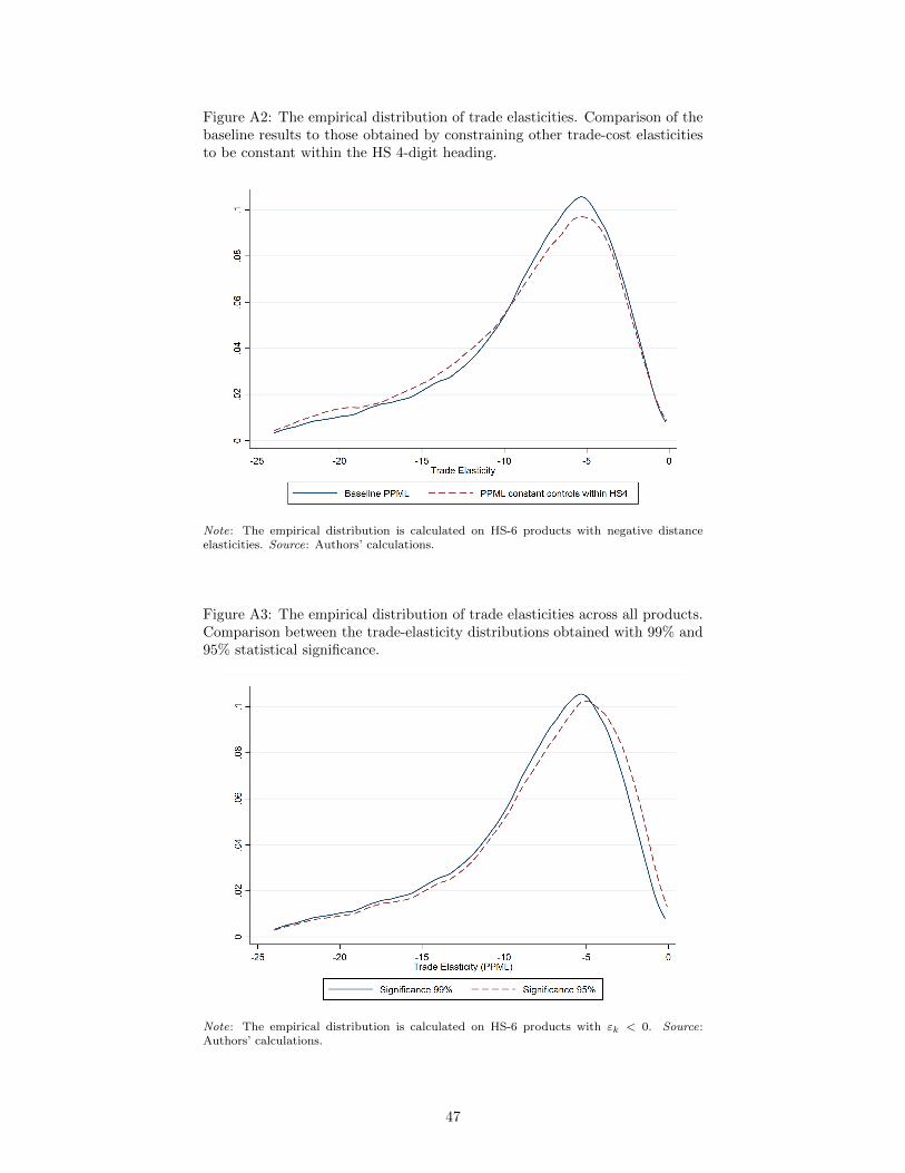
Figure A2: The empirical distribution of trade elasticities. Comparison of thebaseline results to those obtained by constraining other trade-cost elasticitiesto be constant within the HS 4-digit heading.
Note: The empirical distribution is calculated on HS-6 products with negative distanceelasticities. Source: Authors’ calculations.
Figure A3: The empirical distribution of trade elasticities across all products.Comparison between the trade-elasticity distributions obtained with 99% and95% statistical significance.
Note: The empirical distribution is calculated on HS-6 products with εk < 0. Source:Authors’ calculations.
47
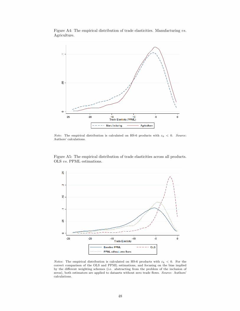
Figure A4: The empirical distribution of trade elasticities. Manufacturing vs.Agriculture.
Note: The empirical distribution is calculated on HS-6 products with εk < 0. Source:Authors’ calculations.
Figure A5: The empirical distribution of trade elasticities across all products.OLS vs. PPML estimations.
Notes: The empirical distribution is calculated on HS-6 products with εk < 0. For thecorrect comparison of the OLS and PPML estimations, and focusing on the bias impliedby the different weighting schemes (i.e. abstracting from the problem of the inclusion ofzeros), both estimators are applied to datasets without zero trade flows. Source: Authors’calculations.
48
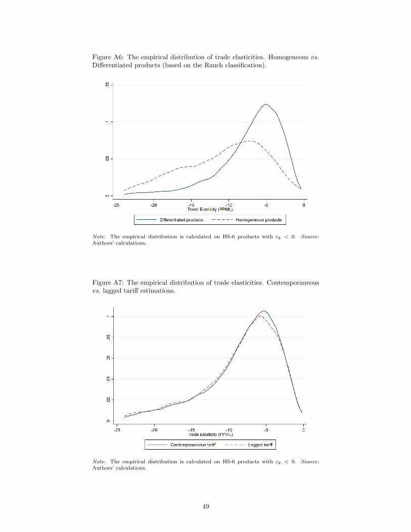
Figure A6: The empirical distribution of trade elasticities. Homogeneous vs.Differentiated products (based on the Rauch classification).
Note: The empirical distribution is calculated on HS-6 products with εk < 0. Source:Authors’ calculations.
Figure A7: The empirical distribution of trade elasticities. Contemporaneousvs. lagged tariff estimations.
Note: The empirical distribution is calculated on HS-6 products with εk < 0. Source:Authors’ calculations.
49
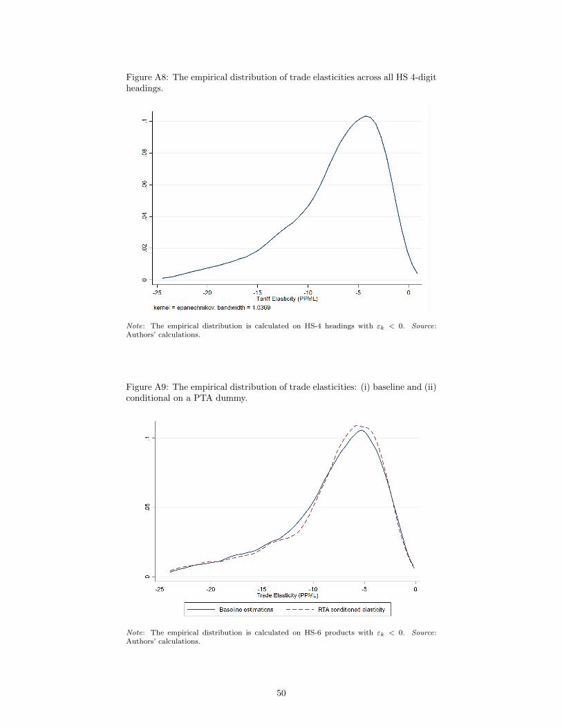
Figure A8: The empirical distribution of trade elasticities across all HS 4-digitheadings.
Note: The empirical distribution is calculated on HS-4 headings with εk < 0. Source:Authors’ calculations.
Figure A9: The empirical distribution of trade elasticities: (i) baseline and (ii)conditional on a PTA dummy.
Note: The empirical distribution is calculated on HS-6 products with εk < 0. Source:Authors’ calculations.
50
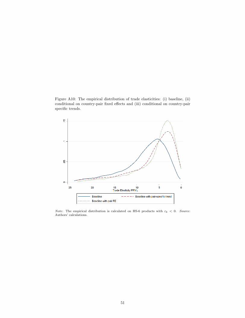
Figure A10: The empirical distribution of trade elasticities: (i) baseline, (ii)conditional on country-pair fixed effects and (iii) conditional on country-pairspecific trends.
Note: The empirical distribution is calculated on HS-6 products with εk < 0. Source:Authors’ calculations.
51
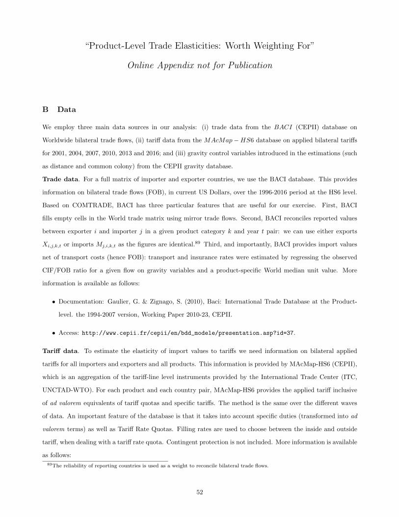
“Product-Level Trade Elasticities: Worth Weighting For”
Online Appendix not for Publication
B Data
We employ three main data sources in our analysis: (i) trade data from the BACI (CEPII) database on
Worldwide bilateral trade flows, (ii) tariff data from the MAcMap−HS6 database on applied bilateral tariffs
for 2001, 2004, 2007, 2010, 2013 and 2016; and (iii) gravity control variables introduced in the estimations (such
as distance and common colony) from the CEPII gravity database.
Trade data. For a full matrix of importer and exporter countries, we use the BACI database. This provides
information on bilateral trade flows (FOB), in current US Dollars, over the 1996-2016 period at the HS6 level.
Based on COMTRADE, BACI has three particular features that are useful for our exercise. First, BACI
fills empty cells in the World trade matrix using mirror trade flows. Second, BACI reconciles reported values
between exporter i and importer j in a given product category k and year t pair: we can use either exports
Xi,j,k,t or imports Mj,i,k,t as the figures are identical.89 Third, and importantly, BACI provides import values
net of transport costs (hence FOB): transport and insurance rates were estimated by regressing the observed
CIF/FOB ratio for a given flow on gravity variables and a product-specific World median unit value. More
information is available as follows:
• Documentation: Gaulier, G. & Zignago, S. (2010), Baci: International Trade Database at the Product-
level. the 1994-2007 version, Working Paper 2010-23, CEPII.
• Access: http://www.cepii.fr/cepii/en/bdd_modele/presentation.asp?id=37.
Tariff data. To estimate the elasticity of import values to tariffs we need information on bilateral applied
tariffs for all importers and exporters and all products. This information is provided by MAcMap-HS6 (CEPII),
which is an aggregation of the tariff-line level instruments provided by the International Trade Center (ITC,
UNCTAD-WTO). For each product and each country pair, MAcMap-HS6 provides the applied tariff inclusive
of ad valorem equivalents of tariff quotas and specific tariffs. The method is the same over the different waves
of data. An important feature of the database is that it takes into account specific duties (transformed into ad
valorem terms) as well as Tariff Rate Quotas. Filling rates are used to choose between the inside and outside
tariff, when dealing with a tariff rate quota. Contingent protection is not included. More information is available
as follows:
89The reliability of reporting countries is used as a weight to reconcile bilateral trade flows.
52
• Documentation: Guimbard, H., Jean, S., Mimouni, M. & Pichot, X. (2012), MAcMap-HS6 2007, an
Exhaustive and Consistent Measure of Applied Protection in 2007, International Economics (130): 99-
122.
• Access: http://www.cepii.fr/cepii/en/bdd_modele/presentation.asp?id=12.
Gravity variables. The common gravity variables such as bilateral distance, common language, border and
colony dummies are taken from the Gravity CEPII database available on line.
• Documentation: Head, K., Mayer, T. & Ries, J. (2010), The Erosion of Colonial Trade Linkages after
Independence, Journal of International Economics, 81(1):1-14
• Access: http://www.cepii.fr/cepii/en/bdd_modele/presentation.asp?id=8.
Construction of the estimation sample. MAcMap-HS6 covers 159 importers for 2001. Subsequent releases
have increased coverage, with the exception of 2010 for which we have only 152 importers. We therefore retain
the sample of the 152 importers that are present in all of the releases of MAcMap-HS6 (the list of importing
countries appears in the Online Appendix Table B1). On the exporting side the constraint is less binding,
and we keep exporters that have been present in BACI since 2001. Ultimately, we have 189 exporters to 152
destinations in each year, and therefore potentially a fully-balanced dataset. However, at the HS6 level the
Worldwide fully-balanced matrix of bilateral trade comprises many zeros, many of which are not relevant for
the identification of the tariff coefficient. In particular, if a given exporting country i never exports a specific
product k, this would be perfectly predicted by the exporter-year fixed effects that always appear in Equation
5. We therefore carry out a fill-in of the World trade matrix with zeros only when country i exports product k
to at least one destination over the period.
53
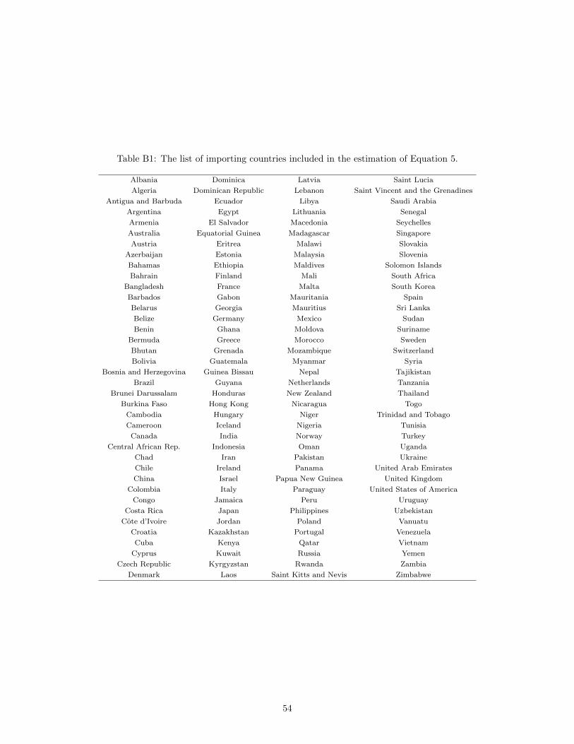
Table B1: The list of importing countries included in the estimation of Equation 5.
Albania Dominica Latvia Saint Lucia
Algeria Dominican Republic Lebanon Saint Vincent and the Grenadines
Antigua and Barbuda Ecuador Libya Saudi Arabia
Argentina Egypt Lithuania Senegal
Armenia El Salvador Macedonia Seychelles
Australia Equatorial Guinea Madagascar Singapore
Austria Eritrea Malawi Slovakia
Azerbaijan Estonia Malaysia Slovenia
Bahamas Ethiopia Maldives Solomon Islands
Bahrain Finland Mali South Africa
Bangladesh France Malta South Korea
Barbados Gabon Mauritania Spain
Belarus Georgia Mauritius Sri Lanka
Belize Germany Mexico Sudan
Benin Ghana Moldova Suriname
Bermuda Greece Morocco Sweden
Bhutan Grenada Mozambique Switzerland
Bolivia Guatemala Myanmar Syria
Bosnia and Herzegovina Guinea Bissau Nepal Tajikistan
Brazil Guyana Netherlands Tanzania
Brunei Darussalam Honduras New Zealand Thailand
Burkina Faso Hong Kong Nicaragua Togo
Cambodia Hungary Niger Trinidad and Tobago
Cameroon Iceland Nigeria Tunisia
Canada India Norway Turkey
Central African Rep. Indonesia Oman Uganda
Chad Iran Pakistan Ukraine
Chile Ireland Panama United Arab Emirates
China Israel Papua New Guinea United Kingdom
Colombia Italy Paraguay United States of America
Congo Jamaica Peru Uruguay
Costa Rica Japan Philippines Uzbekistan
Cote d’Ivoire Jordan Poland Vanuatu
Croatia Kazakhstan Portugal Venezuela
Cuba Kenya Qatar Vietnam
Cyprus Kuwait Russia Yemen
Czech Republic Kyrgyzstan Rwanda Zambia
Denmark Laos Saint Kitts and Nevis Zimbabwe
54
C The comparison to previous estimates of trade elasticities.
As discussed in the introduction, this is not the first paper to provide trade elasticities (although we are the first
to rely on the systematic coverage of exporters and importers at such a detailed level of product disaggregation).
While the distribution of the product-level elasticities obtained here is centered around values that are in line
with those in the literature, the comparison shows more differences when aggregating these elasticities up to
the classifications used in other papers. We now compare our trade-elasticity estimates to those in (i) Caliendo
& Parro (2015),90 (ii) Ossa (2015),91 (iii) Broda et al. (2006)92 and (iv) Kee et al. (2009). We aggregate our
trade elasticities at the HS 3-digit level to compare with those in Broda et al. (2006) and Kee et al. (2009),
at the SITC rev. 3 sector level to compare with Ossa (2015), and at the ISIC 2-digit level to compare with
Caliendo & Parro (2015). We calculate a weighted average of HS6 trade elasticities, using product-export shares
(over World exports) in 2001 as the weights. For the correct comparison with other existing sets of elasticities,
insignificant and missing elasticities have been replaced by the average HS 4-digit specific elasticity. The same
strategy is adopted for the dataset of HS6 elasticities from this paper that has been made available online.
Online Appendix Table C1 shows the simple correlation indices and rank correlations between our estimated
elasticities and those from the four benchmark papers above. Our elasticities are positively (although weakly)
correlated with those in Broda et al. (2006), Caliendo & Parro (2015) and Kee et al. (2009), and essentially
uncorrelated with those in Ossa (2015). Our empirical method differs considerably from that in Broda et al.
(2006), Kee et al. (2009) and Ossa (2015), but more importantly averaging product-level elasticities to produce
sector-level elasticities is very sensitive to the weighting scheme: a simple average would produce a correlation of
0.8 with Caliendo & Parro (2015). This is why we rely in the text on a more accurate strategy: TiVA (and other
sector aggregations) elasticities are computed by pooling HS6 products within the TiVA sectors and estimating
our equation sector by sector.
90See Table 1 in Caliendo & Parro (2015).91https://docs.google.com/viewer?a=v&pid=sites&srcid=ZGVmYXVsdGRvbWFpbnxwcm9mb3NzYXV6aHxneDpiYTU3NmMxZTVlMmE5MGQ.92http://www.columbia.edu/~dew35/TradeElasticities/TradeElasticities.html.
55
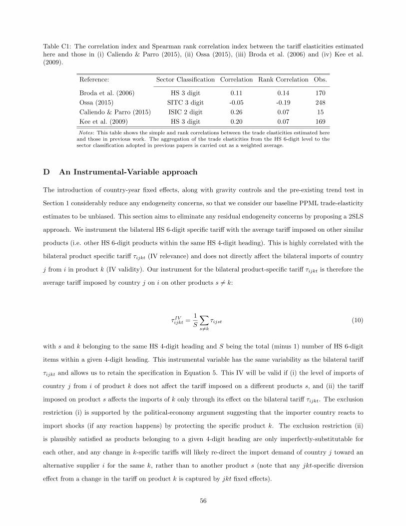
Table C1: The correlation index and Spearman rank correlation index between the tariff elasticities estimatedhere and those in (i) Caliendo & Parro (2015), (ii) Ossa (2015), (iii) Broda et al. (2006) and (iv) Kee et al.(2009).
Reference: Sector Classification Correlation Rank Correlation Obs.
Broda et al. (2006) HS 3 digit 0.11 0.14 170
Ossa (2015) SITC 3 digit -0.05 -0.19 248
Caliendo & Parro (2015) ISIC 2 digit 0.26 0.07 15
Kee et al. (2009) HS 3 digit 0.20 0.07 169
Notes: This table shows the simple and rank correlations between the trade elasticities estimated hereand those in previous work. The aggregation of the trade elasticities from the HS 6-digit level to thesector classification adopted in previous papers is carried out as a weighted average.
D An Instrumental-Variable approach
The introduction of country-year fixed effects, along with gravity controls and the pre-existing trend test in
Section 1 considerably reduce any endogeneity concerns, so that we consider our baseline PPML trade-elasticity
estimates to be unbiased. This section aims to eliminate any residual endogeneity concerns by proposing a 2SLS
approach. We instrument the bilateral HS 6-digit specific tariff with the average tariff imposed on other similar
products (i.e. other HS 6-digit products within the same HS 4-digit heading). This is highly correlated with the
bilateral product specific tariff τijkt (IV relevance) and does not directly affect the bilateral imports of country
j from i in product k (IV validity). Our instrument for the bilateral product-specific tariff τijkt is therefore the
average tariff imposed by country j on i on other products s 6= k:
τ IVijkt =1
S
∑s6=k
τijst (10)
with s and k belonging to the same HS 4-digit heading and S being the total (minus 1) number of HS 6-digit
items within a given 4-digit heading. This instrumental variable has the same variability as the bilateral tariff
τijkt and allows us to retain the specification in Equation 5. This IV will be valid if (i) the level of imports of
country j from i of product k does not affect the tariff imposed on a different products s, and (ii) the tariff
imposed on product s affects the imports of k only through its effect on the bilateral tariff τijkt. The exclusion
restriction (i) is supported by the political-economy argument suggesting that the importer country reacts to
import shocks (if any reaction happens) by protecting the specific product k. The exclusion restriction (ii)
is plausibly satisfied as products belonging to a given 4-digit heading are only imperfectly-substitutable for
each other, and any change in k-specific tariffs will likely re-direct the import demand of country j toward an
alternative supplier i for the same k, rather than to another product s (note that any jkt-specific diversion
effect from a change in the tariff on product k is captured by jkt fixed effects).
56
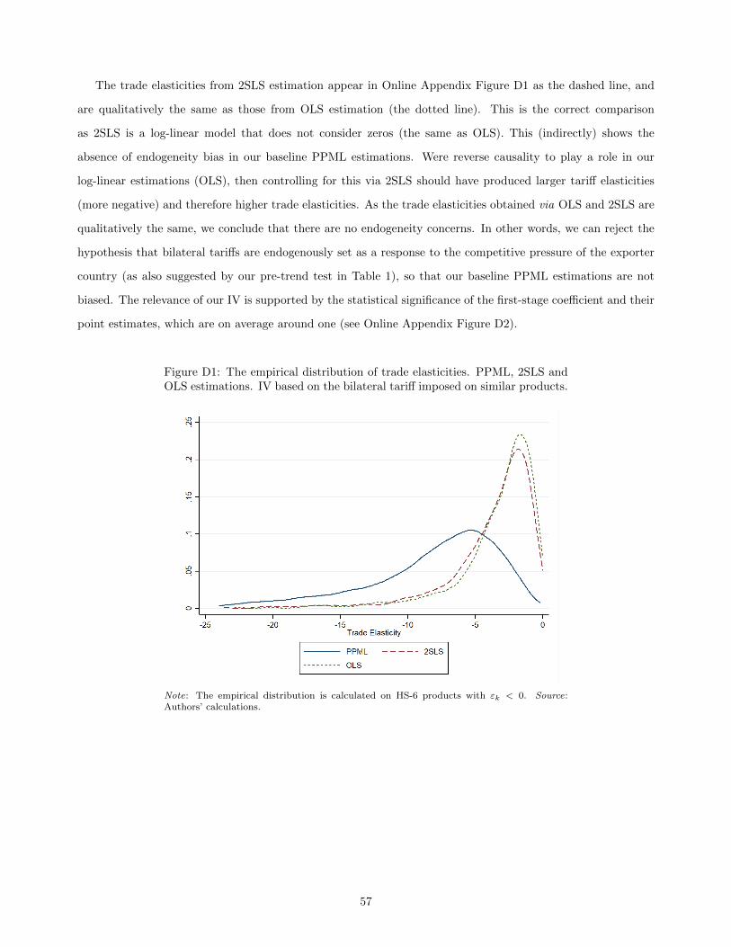
The trade elasticities from 2SLS estimation appear in Online Appendix Figure D1 as the dashed line, and
are qualitatively the same as those from OLS estimation (the dotted line). This is the correct comparison
as 2SLS is a log-linear model that does not consider zeros (the same as OLS). This (indirectly) shows the
absence of endogeneity bias in our baseline PPML estimations. Were reverse causality to play a role in our
log-linear estimations (OLS), then controlling for this via 2SLS should have produced larger tariff elasticities
(more negative) and therefore higher trade elasticities. As the trade elasticities obtained via OLS and 2SLS are
qualitatively the same, we conclude that there are no endogeneity concerns. In other words, we can reject the
hypothesis that bilateral tariffs are endogenously set as a response to the competitive pressure of the exporter
country (as also suggested by our pre-trend test in Table 1), so that our baseline PPML estimations are not
biased. The relevance of our IV is supported by the statistical significance of the first-stage coefficient and their
point estimates, which are on average around one (see Online Appendix Figure D2).
Figure D1: The empirical distribution of trade elasticities. PPML, 2SLS andOLS estimations. IV based on the bilateral tariff imposed on similar products.
Note: The empirical distribution is calculated on HS-6 products with εk < 0. Source:Authors’ calculations.
57
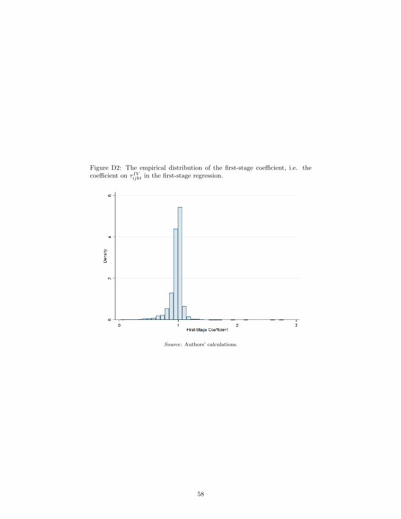
Figure D2: The empirical distribution of the first-stage coefficient, i.e. thecoefficient on τ IVijkt in the first-stage regression.
Source: Authors’ calculations.
58
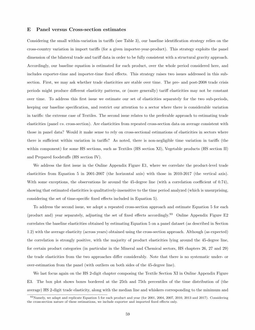
E Panel versus Cross-section estimates
Considering the small within-variation in tariffs (see Table 3), our baseline identification strategy relies on the
cross-country variation in import tariffs (for a given importer-year-product). This strategy exploits the panel
dimension of the bilateral trade and tariff data in order to be fully consistent with a structural gravity approach.
Accordingly, our baseline equation is estimated for each product, over the whole period considered here, and
includes exporter-time and importer-time fixed effects. This strategy raises two issues addressed in this sub-
section. First, we may ask whether trade elasticities are stable over time. The pre- and post-2008 trade crisis
periods might produce different elasticity patterns, or (more generally) tariff elasticities may not be constant
over time. To address this first issue we estimate our set of elasticities separately for the two sub-periods,
keeping our baseline specification, and restrict our attention to a sector where there is considerable variation
in tariffs: the extreme case of Textiles. The second issue relates to the preferable approach to estimating trade
elasticities (panel vs. cross-section). Are elasticities from repeated cross-section data on average consistent with
those in panel data? Would it make sense to rely on cross-sectional estimations of elasticities in sectors where
there is sufficient within variation in tariffs? As noted, there is non-negligible time variation in tariffs (the
within component) for some HS sections, such as Textiles (HS section XI), Vegetable products (HS section II)
and Prepared foodstuffs (HS section IV).
We address the first issue in the Online Appendix Figure E1, where we correlate the product-level trade
elasticities from Equation 5 in 2001-2007 (the horizontal axis) with those in 2010-2017 (the vertical axis).
With some exceptions, the observations lie around the 45-degree line (with a correlation coefficient of 0.74),
showing that estimated elasticities is qualitatively-insensitive to the time period analyzed (which is unsurprising,
considering the set of time-specific fixed effects included in Equation 5).
To address the second issue, we adopt a repeated cross-section approach and estimate Equation 5 for each
(product and) year separately, adjusting the set of fixed effects accordingly.93 Online Appendix Figure E2
correlates the baseline elasticities obtained by estimating Equation 5 on a panel dataset (as described in Section
1.2) with the average elasticity (across years) obtained using the cross-section approach. Although (as expected)
the correlation is strongly positive, with the majority of product elasticities lying around the 45-degree line,
for certain product categories (in particular in the Mineral and Chemical sectors, HS chapters 26, 27 and 29)
the trade elasticities from the two approaches differ considerably. Note that there is no systematic under- or
over-estimation from the panel (with outliers on both sides of the 45-degree line).
We last focus again on the HS 2-digit chapter composing the Textile Section XI in Online Appendix Figure
E3. The box plot shows boxes bordered at the 25th and 75th percentiles of the time distribution of (the
average) HS 2-digit trade elasticity, along with the median line and whiskers corresponding to the minimum and
93Namely, we adapt and replicate Equation 5 for each product and year (for 2001, 2004, 2007, 2010, 2013 and 2017). Consideringthe cross-section nature of these estimations, we include exporter and imported fixed effects only.
59
maximum elasticities. From Online Appendix Figure E3 there is a clear large gap in trade elasticities estimated
by cross-section at different points in time for certain product categories (see for example the Wool, Vegetable
and Textile sectors).
The evidence in Online Appendix Figures E2 and E3 suggests that, although the two empirical approaches
produce on average qualitatively-similar results, there are notable exceptions. This reflects that the Cov(Xjit−
X.jt, Yjit − Y.jt) underlying the panel estimate with fixed effects in Equation 5 is different from the average
Cov(Xji − X.j , Yji − Y.j) used in the cross-section estimate. From a structural interpretation point of view,
these exceptions stress that the cross-section approach, by abstracting from the time dimension, does not prop-
erly capture any exporter (or importer) specific time-varying shocks. For this reason the baseline panel approach
is preferred in the paper.
Figure E1: The correlation between the baseline HS6 trade elasticities esti-mated in the 2001-2007 and 2010-2017 sub-periods (Textile sector, HS sectionXI).
Notes: The empirical distribution is calculated on HS-6 products with εk < 0. Tradeelasticities under -50 are not shown for readability. Source: Authors’ calculations.
60
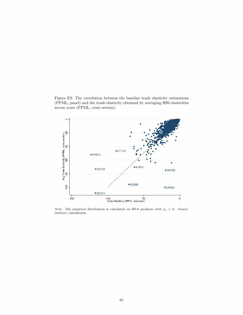
Figure E2: The correlation between the baseline trade elasticity estimations(PPML, panel) and the trade elasticity obtained by averaging HS6 elasticitiesacross years (PPML, cross section).
Note: The empirical distribution is calculated on HS-6 products with εk < 0. Source:Authors’ calculations.
61
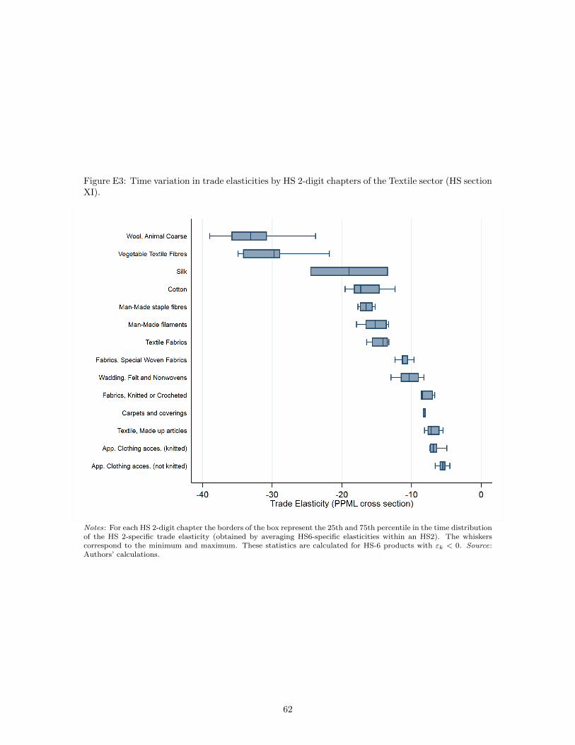
Figure E3: Time variation in trade elasticities by HS 2-digit chapters of the Textile sector (HS sectionXI).
Notes: For each HS 2-digit chapter the borders of the box represent the 25th and 75th percentile in the time distributionof the HS 2-specific trade elasticity (obtained by averaging HS6-specific elasticities within an HS2). The whiskerscorrespond to the minimum and maximum. These statistics are calculated for HS-6 products with εk < 0. Source:Authors’ calculations.
62
F Interpreting positive and insignificant trade elasticities
This section tentatively explains why certain elasticities were not precisely estimated. When estimating Equation
5 for each of the 5,050 HS-6 product lines using the PPML estimator, we obtain a small number of positive and
some insignificant elasticities. These might appear puzzling at first glance, and we here propose some potential
explanations.
Interpreting positive trade elasticities. We obtain positive βk parameters for certain products, implying
positive trade elasticities εk.94 Online Appendix Table F1 shows the descriptive statistics of the share of positive
estimated εk parameters that are statistically significant at the 1% level. This applies to 2.5% of the estimated
εk,95 and these are concentrated in a few very-particular HS 2-digit chapters. Online Appendix Table F1 lists
the HS 2-digit chapters in which the frequency of positive εk coefficients is above the mean. Organic chemicals,
Inorganic chemicals, and Nuclear reactors represent almost half of the total number of positive εk elasticities in
this Table.96 While in certain sectors, such as Nuclear reactors, we may not expect the usual market forces to
apply, in others, like Chemicals, these positive trade elasticities deserve further scrutiny. When prices do not
determine quantities, we should consider departures from monopolistically-competitive equilibrium. But here
a lack of competition does not suffice to explain the reversal of the sign of the trade elasticity. We therefore
consider an alternative explanation based on a general-equilibrium argument.
Let us first focus on market structures as an explanation for positive elasticities. Although these only
represent 2.5% of the total sample of significant elasticities, we would like to characterize the product categories
concerned. We thus adopt a purely heuristic approach and run a probit regression for having a positive trade
elasticity (when the underlying tariff coefficient is positive) - P[εk > 0|βk>0] - using market-structure proxies:
P[εk > 0|βk>0] = δ1Xk + δ2Mk + δ3XMk + δ4Kk + εk (11)
In Equation 11 the probability of a positive and significant (at the 1% level) trade elasticity for a given product
k from Equation 5 depends on four sets of covariates: (i) exporters’ characteristics in the international trade
of product k (Xk); (ii) importers’ characteristics (Mk); (iii) country-pair characteristics in the international
trade of product k (XMk); and (iv) product-specific characteristics (Kk). The set of covariates Xk includes
94A positive trade elasticity may also come about with small tariff elasticities, i.e. −1 < βk < 0. However, this is only the casefor one HS6 product.
95This figure rises to 4.3% and 6% respectively at the 5% and 10% significance levels. In the analysis that follows, and in thedataset we provide, we keep 1% significant εk only. The trade elasticities with insignificant tariff coefficients are set to zero (asthey are statistically not different from zero). In the published version of the database, each positive HS6 εk coefficient is replacedby the average εk of its HS-4 heading (the average across negative HS-6 specific εk within the HS4). The products concerned areflagged. The database therefore contains five variables: (i) the HS6 product category, (ii) the value of the trade elasticity εk, (iii)a dummy for the εk coefficient from the original estimation actually being one (i.e. an insignificant tariff elasticity), (iv) a dummyfor the εk from the original estimation being positive or (v) missing.
96The presence of numerous anti-dumping duties for Organic and Inorganic chemicals may help explain this outcome: in thepresence of a binding overhang, imposing countries may increase their applied tariff up to the bound tariff in order to compensatefor the phasing out of the anti-dumping duty, hence generating simultaneous rises in tariff and imports.
63
the number of exporting countries in a specific k, their concentration (measured by a Herfindahl-Hirschmann
index), and the average per capita GDP (weighted by total exports) of the exporter - here intended as a proxy
for the technical level/quality of the exported products. Symmetrically, the set of covariates Mk includes the
same variables but from the perspective of the importing countries. The vector XMk includes the number of
exporter-importer pairs with zero-trade flows for a given k, and the average exporter-importer distance covered
by a product in its international trade matrix (tentatively accounting for sorting effects in relation to trade
costs).97 Last, the set of product-specific covariates Kk includes a dummy for differentiated vs. homogeneous
products and, importantly, the average HS 4-digit applied worldwide bilateral tariff.98
The results in Online Appendix Table F2 show the empirical regularities behind the observed deviations
from the monopolistically-competitive equilibrium for certain product categories. First, products k with a
highly-concentrated set of exporters and/or importers (as revealed by the HH index) are more likely to have
positive tariff elasticities, and therefore trade elasticities εk > 0. With substantial market concentration, higher
tariffs at destination may lead to unexpected results: the deterioration of market access at destination may
push incumbent exporters to exert even greater effort to secure their presence at destination. In a model of
imperfect competition and variable markups, firms reduce their markups and thus export prices when they
lose market share (Atkeson & Burstein 2008). This yields a negative relationship between tariffs and export
prices (see Fontagne et al. 2018), which may partially offset the direct negative tariff effect on exports. A
second regularity in Online Appendix Table F2 is the positive correlation between the average income of ex-
porters and importers and the probability of obtaining positive trade (and tariff) elasticities. On the exporter
side this mirrors the technological level of goods, while on the importing side this is in line with the recent
literature on non-homothetic preferences (Markusen 2013), in which markups rise with destination per capita
income (Bertoletti, Etro & Simonovska 2018). But again, this would not explain the positive impact of tariffs
on demand for a given quality of the imported good. Some unobserved general-equilibrium effect is likely at
play. In order to address this general-equilibrium issue, we observe the impact of tariffs on other goods within
the same broad category. We obtain a positive (although weakly-significant) coefficient on average HS 4-digit
tariffs: as the tariff on another similar product s 6= k increases (here captured by the average tariff in the HS4
chapter), imports of j may rise even though j’s import tariff is higher as a result of the substitution of j with s.99
97We consider here the average distance across country-pairs in a given product k, weighted by trade flows. As the estimatedelasticity ε does not vary over time, all of the explanatory variables have been expressed as averages over the time period.
98Given the large chunk of positive trade elasticities in the Nuclear-reactors sector (HS 84), we re-estimated Equation 11 excludingHS chapter 84: the results do not change.
99This argument should not be confused with the IV exclusion-restriction assumption discussed in Online Appendix Section D.For the validity of our IV we (plausibly) assume the absence of substitution effect across HS6 products (of a given HS4 heading)within the ij trade relationship: when country j raises its tariff on product k exported by i, the demand for k will then likelybe diverted towards a new supplier n 6= i of that product (rather than towards some imperfect substitute for k produced by i).Here, as a potential explanation for the lack of reaction of the demand for product k to a change in tariffs, we assume that there issubstitutability between the HS6 products in a given HS4 heading. As such, when the average tariff on some HS6 product over allij country pairs rises, the demand for this product switches to another product within the same HS4 heading.
64
Interpreting insignificant trade elasticities. The same proxies for market structure used to estimate
Equation 11 may also explain our insignificant tariff coefficients. Columns 3-4 of Online Appendix Table F2
show the results from Equation 11, where the dependent variable is the probability of an insignificant underlying
tariff elasticity, i.e. P[βk = 0].
Columns (3)-(4) of Online Appendix Table F2 reveal a positive correlation between insignificant tariff elas-
ticities and the average income of exporting and importing countries. Similarly, there is a positive correlation
between the average distance covered by a product and the probability of an insignificant tariff elasticity. Al-
though these results are consistent with high-quality products often being characterized by low elasticities of
substitution (Hummels & Skiba 2004) they might also reflect a statistical problem: developed countries have
low tariffs on average and little variation in these tariffs, making it difficult to estimate the tariff coefficient.
Also, in line with intuition, columns (3)-(4) reveal that the demand for differentiated products is relatively
insensitive to tariffs, as shown here by the positive and significant impact of differentiation on the probability
of an insignificant βk estimate on the tariff variable in our baseline equation.
Last, columns (3) and (4) of Online Appendix Table F2 illustrate the intrinsic difficulties of trade-elasticity
estimation based on tariff changes. First, we observe that the presence of zero trade flows for a given product
(and so limited variation in the dependent variable) increases the probability of an insignificant βk estimate.
Second, this probability falls with the number of exporting countries of a given product. This is consistent, as
we exploit the variation in the bilateral tariff imposed by importers on the different exporters of the product: all
else equal, the variation in the tariff is expected to rise in the number of exporters, making it easier to estimate
precisely the parameter of interest. Despite these intrinsic obstacles, our estimations perform fairly well, as
testified by the only small number of positive or insignificant βk estimates.
65
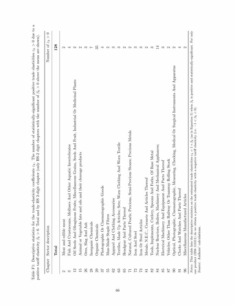
Tab
leF
1:D
escr
ipti
vest
atis
tics
for
the
trad
e-el
asti
city
coeffi
cien
tsε k
.T
he
nu
mb
erof
stati
stic
all
y-s
ign
ifica
nt
posi
tive
trad
eel
ast
icit
iesε k>
0d
ue
toa
pos
itiv
eta
riff
elas
tici
tyβk>
0.T
otal
and
by
HS
2-d
igit
chap
ter
(on
lyH
S-2
dig
itch
ap
ters
wit
hth
enum
ber
ofβk>
0ab
ove
the
mea
nare
show
n).
Ch
apte
rS
ecto
rd
escr
ipti
onN
um
ber
ofε k>
0
Tota
l128
2M
eat
and
edib
lem
eat
2
3F
ish
An
dC
rust
acea
ns,
Mol
lusc
sA
nd
Oth
erA
qu
ati
cIn
vert
ebra
tes
4
12O
ilS
eed
sA
nd
Ole
agin
ous
Fru
its;
Mis
cell
an
eou
sG
rain
s,S
eed
sA
nd
Fru
it,
Ind
ust
rial
Or
Med
icin
al
Pla
nts
2
15A
nim
alor
Veg
etab
lefa
tsan
doi
lsan
dth
eir
clea
vage
pro
du
cts
2
26O
res,
Sla
gA
nd
Ash
3
28In
orga
nic
Ch
emic
als
7
29O
rgan
icC
hem
ical
s35
37P
hot
ogra
ph
icO
rC
inem
atog
rap
hic
Good
s4
55M
an-M
ade
Sta
ple
Fib
res
2
62A
pp
arel
An
dC
loth
ing
Acc
esso
ries
3
63T
exti
les,
Mad
eU
pA
rtic
les;
Set
s;W
orn
Clo
thin
gA
nd
Worn
Tex
tile
3
65H
ead
gear
An
dP
arts
Th
ereo
f2
71N
atu
ral,
Cu
ltu
red
Pea
rls;
Pre
ciou
s,S
emi-
Pre
ciou
sS
ton
es;
Pre
ciou
sM
etals
2
72Ir
onA
nd
Ste
el3
73Ir
onO
rS
teel
Art
icle
s3
81M
etal
s;N
.E.C
.,C
erm
ets
An
dA
rtic
les
Th
ereo
f2
82T
ool
s,Im
ple
men
ts,
Cu
tler
y,S
poon
sA
nd
Fork
s,O
fB
ase
Met
al
3
84N
ucl
ear
Rea
ctor
s,B
oile
rs,
Mac
hin
ery
An
dM
echan
ical
Ap
pli
an
ces;
14
85E
lect
rica
lM
ach
iner
yA
nd
Equ
ipm
ent
An
dP
art
sT
her
eof
3
87V
ehic
les;
Oth
erT
han
Rai
lway
Or
Tra
mw
ayR
oll
ing
Sto
ck2
90O
pti
cal,
Ph
otog
raph
ic,
Cin
emat
ogra
ph
ic,
Mea
suri
ng,
Ch
eckin
g,
Med
ical
Or
Su
rgic
al
Inst
rum
ents
An
dA
pp
ara
tus
2
91C
lock
sA
nd
Wat
ches
An
dP
arts
Th
ereo
f4
96M
isce
llan
eou
sM
anu
fact
ure
dA
rtic
les
2
Notes:
Th
ista
ble
list
sth
ed
escr
ipti
ve
stati
stic
son
the
esti
mate
dtr
ad
eel
ast
icit
iesε k
=1
+βk
(as
inE
qu
ati
on
5)
wh
enβk
isp
osi
tive
an
dst
ati
stic
ally-s
ign
ifica
nt.
For
on
lyon
ep
rod
uct
(HS
6151011)
do
we
ob
tain
ap
osi
tive
trad
eel
ast
icit
yw
ith
an
egati
ve
tari
ffel
ast
icit
y(i
.e.−
1<βk<
0).
Source:
Auth
ors
’ca
lcula
tions.
66
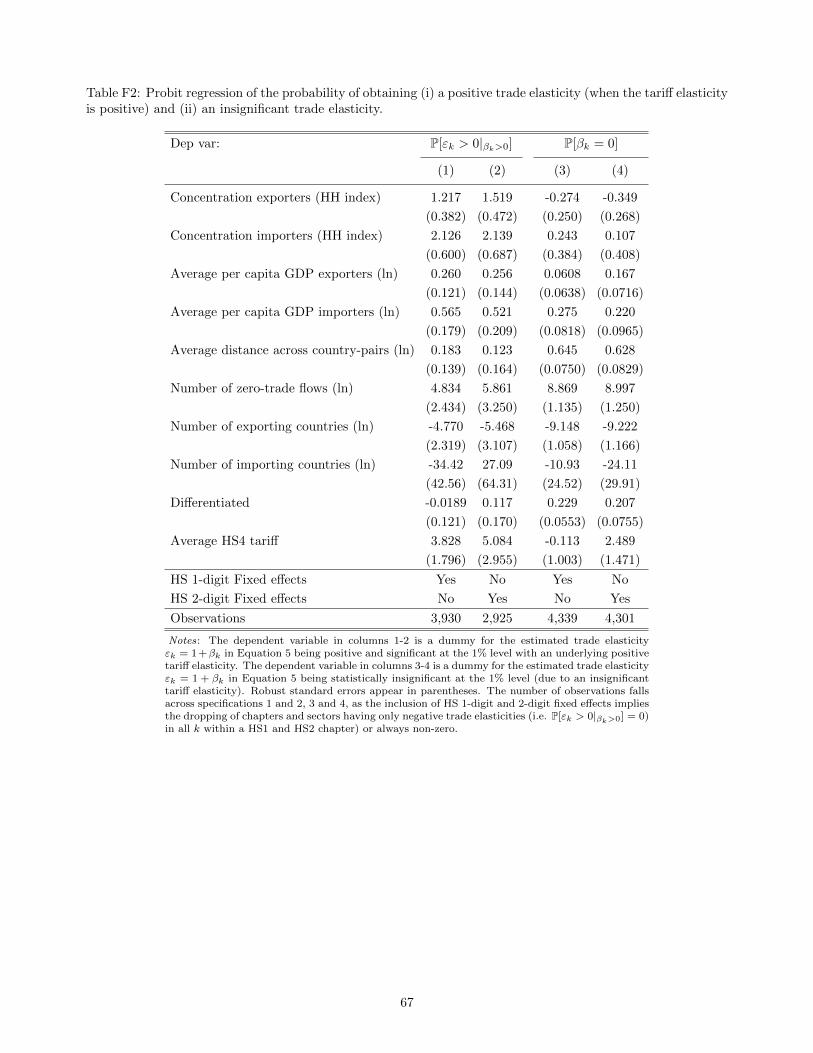
Table F2: Probit regression of the probability of obtaining (i) a positive trade elasticity (when the tariff elasticityis positive) and (ii) an insignificant trade elasticity.
Dep var: P[εk > 0|βk>0] P[βk = 0]
(1) (2) (3) (4)
Concentration exporters (HH index) 1.217 1.519 -0.274 -0.349
(0.382) (0.472) (0.250) (0.268)
Concentration importers (HH index) 2.126 2.139 0.243 0.107
(0.600) (0.687) (0.384) (0.408)
Average per capita GDP exporters (ln) 0.260 0.256 0.0608 0.167
(0.121) (0.144) (0.0638) (0.0716)
Average per capita GDP importers (ln) 0.565 0.521 0.275 0.220
(0.179) (0.209) (0.0818) (0.0965)
Average distance across country-pairs (ln) 0.183 0.123 0.645 0.628
(0.139) (0.164) (0.0750) (0.0829)
Number of zero-trade flows (ln) 4.834 5.861 8.869 8.997
(2.434) (3.250) (1.135) (1.250)
Number of exporting countries (ln) -4.770 -5.468 -9.148 -9.222
(2.319) (3.107) (1.058) (1.166)
Number of importing countries (ln) -34.42 27.09 -10.93 -24.11
(42.56) (64.31) (24.52) (29.91)
Differentiated -0.0189 0.117 0.229 0.207
(0.121) (0.170) (0.0553) (0.0755)
Average HS4 tariff 3.828 5.084 -0.113 2.489
(1.796) (2.955) (1.003) (1.471)
HS 1-digit Fixed effects Yes No Yes No
HS 2-digit Fixed effects No Yes No Yes
Observations 3,930 2,925 4,339 4,301
Notes: The dependent variable in columns 1-2 is a dummy for the estimated trade elasticityεk = 1+βk in Equation 5 being positive and significant at the 1% level with an underlying positivetariff elasticity. The dependent variable in columns 3-4 is a dummy for the estimated trade elasticityεk = 1 + βk in Equation 5 being statistically insignificant at the 1% level (due to an insignificanttariff elasticity). Robust standard errors appear in parentheses. The number of observations fallsacross specifications 1 and 2, 3 and 4, as the inclusion of HS 1-digit and 2-digit fixed effects impliesthe dropping of chapters and sectors having only negative trade elasticities (i.e. P[εk > 0|βk>0] = 0)in all k within a HS1 and HS2 chapter) or always non-zero.
67
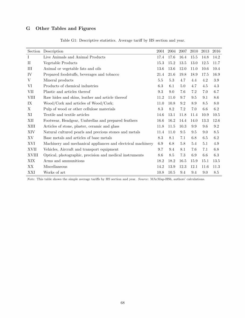
G Other Tables and Figures
Table G1: Descriptive statistics. Average tariff by HS section and year.
Section Description 2001 2004 2007 2010 2013 2016
I Live Animals and Animal Products 17.4 17.6 16.4 15.5 14.8 14.2
II Vegetable Products 15.3 15.2 13.5 13.0 12.5 11.7
III Animal or vegetable fats and oils 13.6 13.6 12.0 11.0 10.6 10.4
IV Prepared foodstuffs, beverages and tobacco 21.4 21.6 19.8 18.9 17.5 16.9
V Mineral products 5.5 5.3 4.7 4.4 4.2 3.9
VI Products of chemical industries 6.3 6.1 5.0 4.7 4.5 4.3
VII Plastic and articles thereof 9.3 9.0 7.6 7.2 7.0 6.7
VIII Raw hides and skins, leather and article thereof 11.2 11.0 9.7 9.5 9.1 8.6
IX Wood/Cork and articles of Wood/Cork; 11.0 10.8 9.2 8.9 8.5 8.0
X Pulp of wood or other cellulose materials 8.3 8.2 7.2 7.0 6.6 6.2
XI Textile and textile articles 14.6 13.1 11.8 11.4 10.9 10.5
XII Footwear, Headgear, Umbrellas and prepared feathers 16.6 16.2 14.4 14.0 13.3 12.6
XIII Articles of stone, plaster, ceramic and glass 11.8 11.5 10.3 9.9 9.6 9.2
XIV Natural cultured pearls and precious stones and metals 11.4 11.0 9.5 9.5 9.0 8.5
XV Base metals and articles of base metals 8.3 8.1 7.1 6.8 6.5 6.2
XVI Machinery and mechanical appliances and electrical machinery 6.9 6.8 5.8 5.4 5.1 4.9
XVII Vehicles, Aircraft and transport equipment 9.7 9.4 8.1 7.6 7.1 6.8
XVIII Optical, photographic, precision and medical instruments 8.6 8.5 7.3 6.9 6.6 6.3
XIX Arms and ammunitions 18.2 18.2 16.5 15.9 15.1 13.5
XX Miscellaneous 14.2 13.9 12.3 12.1 11.6 11.3
XXI Works of art 10.8 10.5 9.4 9.4 9.0 8.5
Note: This table shows the simple average tariffs by HS section and year. Source: MAcMap-HS6, authors’ calculations.
68
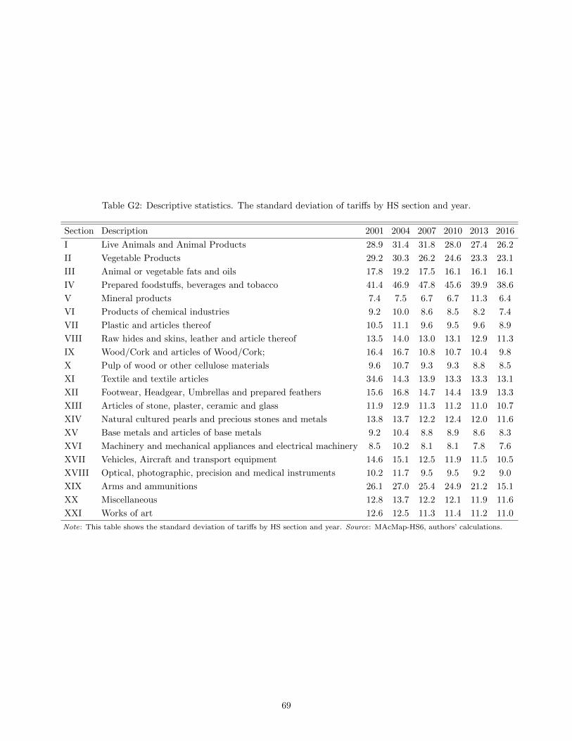
Table G2: Descriptive statistics. The standard deviation of tariffs by HS section and year.
Section Description 2001 2004 2007 2010 2013 2016
I Live Animals and Animal Products 28.9 31.4 31.8 28.0 27.4 26.2
II Vegetable Products 29.2 30.3 26.2 24.6 23.3 23.1
III Animal or vegetable fats and oils 17.8 19.2 17.5 16.1 16.1 16.1
IV Prepared foodstuffs, beverages and tobacco 41.4 46.9 47.8 45.6 39.9 38.6
V Mineral products 7.4 7.5 6.7 6.7 11.3 6.4
VI Products of chemical industries 9.2 10.0 8.6 8.5 8.2 7.4
VII Plastic and articles thereof 10.5 11.1 9.6 9.5 9.6 8.9
VIII Raw hides and skins, leather and article thereof 13.5 14.0 13.0 13.1 12.9 11.3
IX Wood/Cork and articles of Wood/Cork; 16.4 16.7 10.8 10.7 10.4 9.8
X Pulp of wood or other cellulose materials 9.6 10.7 9.3 9.3 8.8 8.5
XI Textile and textile articles 34.6 14.3 13.9 13.3 13.3 13.1
XII Footwear, Headgear, Umbrellas and prepared feathers 15.6 16.8 14.7 14.4 13.9 13.3
XIII Articles of stone, plaster, ceramic and glass 11.9 12.9 11.3 11.2 11.0 10.7
XIV Natural cultured pearls and precious stones and metals 13.8 13.7 12.2 12.4 12.0 11.6
XV Base metals and articles of base metals 9.2 10.4 8.8 8.9 8.6 8.3
XVI Machinery and mechanical appliances and electrical machinery 8.5 10.2 8.1 8.1 7.8 7.6
XVII Vehicles, Aircraft and transport equipment 14.6 15.1 12.5 11.9 11.5 10.5
XVIII Optical, photographic, precision and medical instruments 10.2 11.7 9.5 9.5 9.2 9.0
XIX Arms and ammunitions 26.1 27.0 25.4 24.9 21.2 15.1
XX Miscellaneous 12.8 13.7 12.2 12.1 11.9 11.6
XXI Works of art 12.6 12.5 11.3 11.4 11.2 11.0
Note: This table shows the standard deviation of tariffs by HS section and year. Source: MAcMap-HS6, authors’ calculations.
69
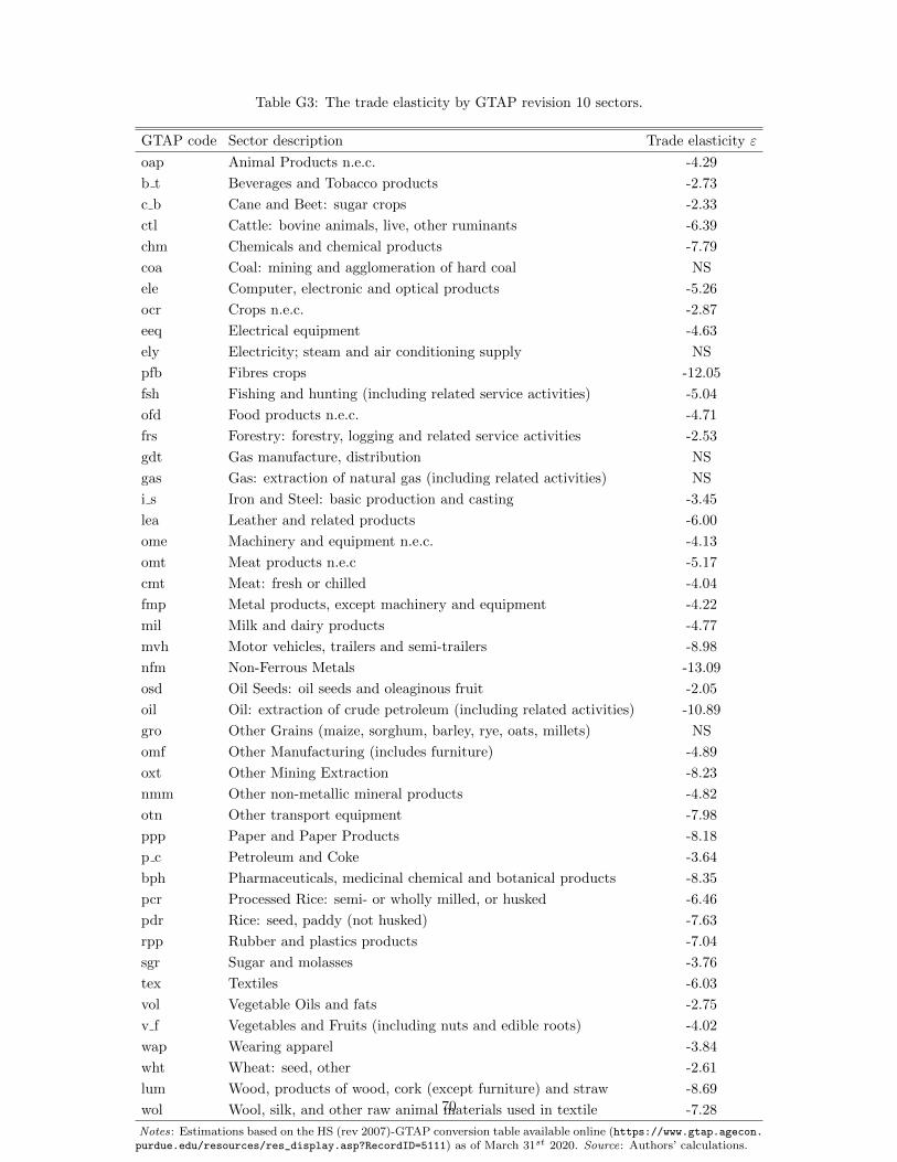
Table G3: The trade elasticity by GTAP revision 10 sectors.
GTAP code Sector description Trade elasticity ε
oap Animal Products n.e.c. -4.29
b t Beverages and Tobacco products -2.73
c b Cane and Beet: sugar crops -2.33
ctl Cattle: bovine animals, live, other ruminants -6.39
chm Chemicals and chemical products -7.79
coa Coal: mining and agglomeration of hard coal NS
ele Computer, electronic and optical products -5.26
ocr Crops n.e.c. -2.87
eeq Electrical equipment -4.63
ely Electricity; steam and air conditioning supply NS
pfb Fibres crops -12.05
fsh Fishing and hunting (including related service activities) -5.04
ofd Food products n.e.c. -4.71
frs Forestry: forestry, logging and related service activities -2.53
gdt Gas manufacture, distribution NS
gas Gas: extraction of natural gas (including related activities) NS
i s Iron and Steel: basic production and casting -3.45
lea Leather and related products -6.00
ome Machinery and equipment n.e.c. -4.13
omt Meat products n.e.c -5.17
cmt Meat: fresh or chilled -4.04
fmp Metal products, except machinery and equipment -4.22
mil Milk and dairy products -4.77
mvh Motor vehicles, trailers and semi-trailers -8.98
nfm Non-Ferrous Metals -13.09
osd Oil Seeds: oil seeds and oleaginous fruit -2.05
oil Oil: extraction of crude petroleum (including related activities) -10.89
gro Other Grains (maize, sorghum, barley, rye, oats, millets) NS
omf Other Manufacturing (includes furniture) -4.89
oxt Other Mining Extraction -8.23
nmm Other non-metallic mineral products -4.82
otn Other transport equipment -7.98
ppp Paper and Paper Products -8.18
p c Petroleum and Coke -3.64
bph Pharmaceuticals, medicinal chemical and botanical products -8.35
pcr Processed Rice: semi- or wholly milled, or husked -6.46
pdr Rice: seed, paddy (not husked) -7.63
rpp Rubber and plastics products -7.04
sgr Sugar and molasses -3.76
tex Textiles -6.03
vol Vegetable Oils and fats -2.75
v f Vegetables and Fruits (including nuts and edible roots) -4.02
wap Wearing apparel -3.84
wht Wheat: seed, other -2.61
lum Wood, products of wood, cork (except furniture) and straw -8.69
wol Wool, silk, and other raw animal materials used in textile -7.28
Notes: Estimations based on the HS (rev 2007)-GTAP conversion table available online (https://www.gtap.agecon.purdue.edu/resources/res_display.asp?RecordID=5111) as of March 31st 2020. Source: Authors’ calculations.
70
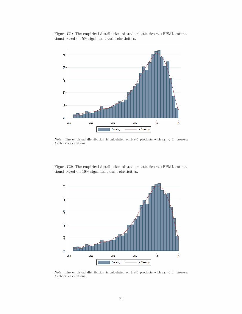
Figure G1: The empirical distribution of trade elasticities εk (PPML estima-tions) based on 5% significant tariff elasticities.
Note: The empirical distribution is calculated on HS-6 products with εk < 0. Source:Authors’ calculations.
Figure G2: The empirical distribution of trade elasticities εk (PPML estima-tions) based on 10% significant tariff elasticities.
Note: The empirical distribution is calculated on HS-6 products with εk < 0. Source:Authors’ calculations.
71
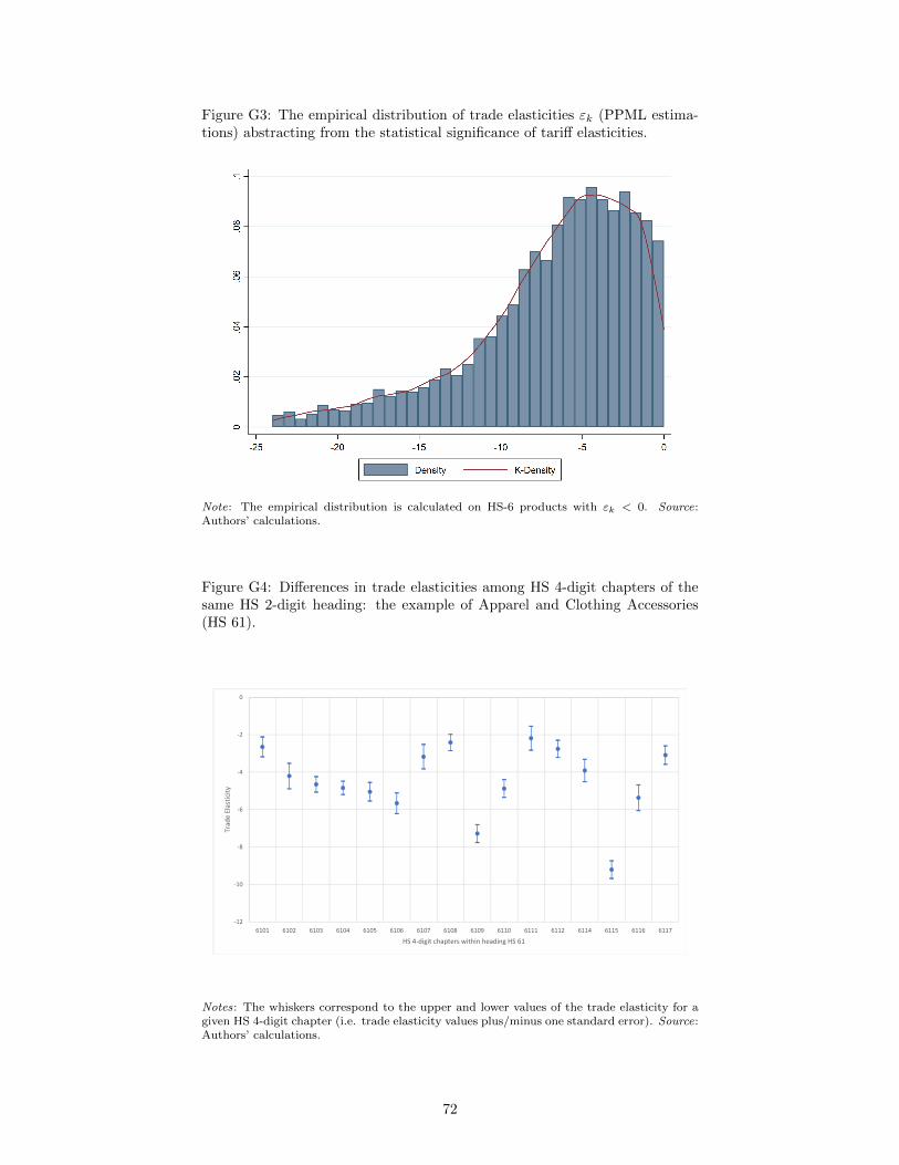
Figure G3: The empirical distribution of trade elasticities εk (PPML estima-tions) abstracting from the statistical significance of tariff elasticities.
Note: The empirical distribution is calculated on HS-6 products with εk < 0. Source:Authors’ calculations.
Figure G4: Differences in trade elasticities among HS 4-digit chapters of thesame HS 2-digit heading: the example of Apparel and Clothing Accessories(HS 61).
-12
-10
-8
-6
-4
-2
0
6101 6102 6103 6104 6105 6106 6107 6108 6109 6110 6111 6112 6114 6115 6116 6117
Tra
de
Ela
stic
ity
HS 4-digit chapters within heading HS 61
Notes: The whiskers correspond to the upper and lower values of the trade elasticity for agiven HS 4-digit chapter (i.e. trade elasticity values plus/minus one standard error). Source:Authors’ calculations.
72
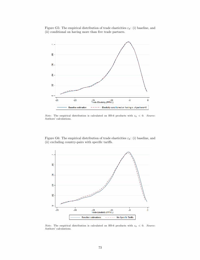
Figure G5: The empirical distribution of trade elasticities εk: (i) baseline, and(ii) conditional on having more than five trade partners.
Note: The empirical distribution is calculated on HS-6 products with εk < 0. Source:Authors’ calculations.
Figure G6: The empirical distribution of trade elasticities εk: (i) baseline, and(ii) excluding country-pairs with specific tariffs.
Note: The empirical distribution is calculated on HS-6 products with εk < 0. Source:Authors’ calculations.
73
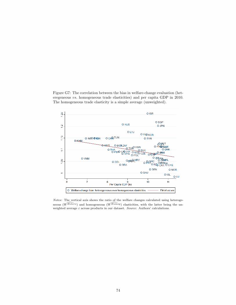
Figure G7: The correlation between the bias in welfare-change evaluation (het-eregeneous vs. homogeneous trade elasticities) and per capita GDP in 2010.The homogeneous trade elasticity is a simple average (unweighted).
Notes: The vertical axis shows the ratio of the welfare changes calculated using heteroge-
neous ( WHetero) and homogeneous ( WHomog) elasticities, with the latter being the un-weighted average ε across products in our dataset. Source: Authors’ calculations.
74
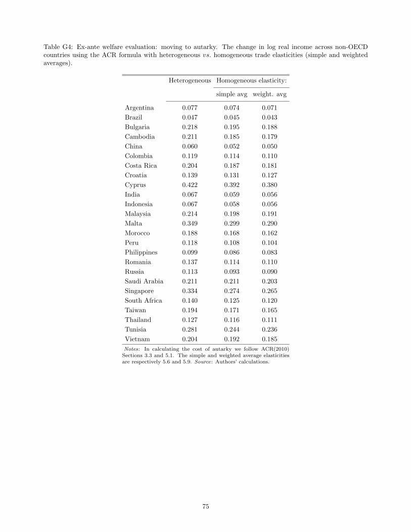
Table G4: Ex-ante welfare evaluation: moving to autarky. The change in log real income across non-OECDcountries using the ACR formula with heterogeneous vs. homogeneous trade elasticities (simple and weightedaverages).
Heterogeneous Homogeneous elasticity:
simple avg weight. avg
Argentina 0.077 0.074 0.071
Brazil 0.047 0.045 0.043
Bulgaria 0.218 0.195 0.188
Cambodia 0.211 0.185 0.179
China 0.060 0.052 0.050
Colombia 0.119 0.114 0.110
Costa Rica 0.204 0.187 0.181
Croatia 0.139 0.131 0.127
Cyprus 0.422 0.392 0.380
India 0.067 0.059 0.056
Indonesia 0.067 0.058 0.056
Malaysia 0.214 0.198 0.191
Malta 0.349 0.299 0.290
Morocco 0.188 0.168 0.162
Peru 0.118 0.108 0.104
Philippines 0.099 0.086 0.083
Romania 0.137 0.114 0.110
Russia 0.113 0.093 0.090
Saudi Arabia 0.211 0.211 0.203
Singapore 0.334 0.274 0.265
South Africa 0.140 0.125 0.120
Taiwan 0.194 0.171 0.165
Thailand 0.127 0.116 0.111
Tunisia 0.281 0.244 0.236
Vietnam 0.204 0.192 0.185
Notes: In calculating the cost of autarky we follow ACR(2010)Sections 3.3 and 5.1. The simple and weighted average elasticitiesare respectively 5.6 and 5.9. Source: Authors’ calculations.
75
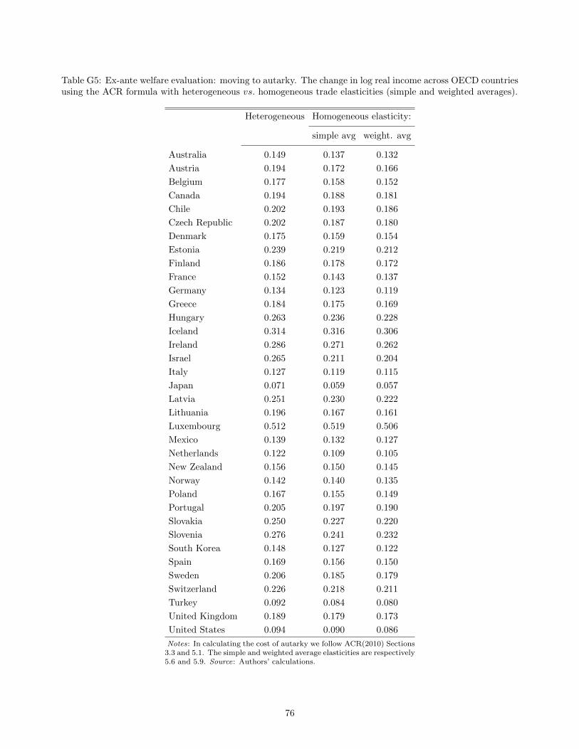
Table G5: Ex-ante welfare evaluation: moving to autarky. The change in log real income across OECD countriesusing the ACR formula with heterogeneous vs. homogeneous trade elasticities (simple and weighted averages).
Heterogeneous Homogeneous elasticity:
simple avg weight. avg
Australia 0.149 0.137 0.132
Austria 0.194 0.172 0.166
Belgium 0.177 0.158 0.152
Canada 0.194 0.188 0.181
Chile 0.202 0.193 0.186
Czech Republic 0.202 0.187 0.180
Denmark 0.175 0.159 0.154
Estonia 0.239 0.219 0.212
Finland 0.186 0.178 0.172
France 0.152 0.143 0.137
Germany 0.134 0.123 0.119
Greece 0.184 0.175 0.169
Hungary 0.263 0.236 0.228
Iceland 0.314 0.316 0.306
Ireland 0.286 0.271 0.262
Israel 0.265 0.211 0.204
Italy 0.127 0.119 0.115
Japan 0.071 0.059 0.057
Latvia 0.251 0.230 0.222
Lithuania 0.196 0.167 0.161
Luxembourg 0.512 0.519 0.506
Mexico 0.139 0.132 0.127
Netherlands 0.122 0.109 0.105
New Zealand 0.156 0.150 0.145
Norway 0.142 0.140 0.135
Poland 0.167 0.155 0.149
Portugal 0.205 0.197 0.190
Slovakia 0.250 0.227 0.220
Slovenia 0.276 0.241 0.232
South Korea 0.148 0.127 0.122
Spain 0.169 0.156 0.150
Sweden 0.206 0.185 0.179
Switzerland 0.226 0.218 0.211
Turkey 0.092 0.084 0.080
United Kingdom 0.189 0.179 0.173
United States 0.094 0.090 0.086
Notes: In calculating the cost of autarky we follow ACR(2010) Sections3.3 and 5.1. The simple and weighted average elasticities are respectively5.6 and 5.9. Source: Authors’ calculations.
76