Product Line Rivalry: How Box Office Revenue Cycles Influence Movie Exhibition Variety**

Darlene C. Chisholm, Department of Economics,

Suffolk University, Boston, MA 02108

George Norman, Department of Economics,

Tufts University, Medford, MA 02155

September 2007

Abstract

We analyze how product line rivalry by multi-product oligopolists is affected by market size and product substitutability. We show that the width and degree of overlap in competing product lines is determined by the tension between two effects: the drive to “be where the demand is” and the desire to weaken competition and intra-firm product cannibalization. Product lines are shown to be wider and more overlapped in large markets and when product substitutability is weak. We provide econometric support for our main hypotheses using data on weekly film programming choices by first-run movie theatres in a large US metropolitan market. Keywords: Product line rivalry; market size; product substitutability; movie exhibition JEL Codes: D21, D43; L13; L82

**We are grateful to the DeSantis Center for Motion Picture Industry Studies of Florida Atlantic University College of Business and Economics for providing a grant to fund this research and to Synergy Retail for compiling data used in this paper. For valuable comments and suggestions, we thank participants at the International Industrial Organization Conference and the DeSantis Center Summit Workshop at Florida Atlantic University. We are grateful to Vicky Huang, Anna Kumysh, and Vidisha Vachharajani for their careful research assistance and to Sorin Codreanu for his data-management programming assistance.

2

1. Introduction

We analyze the impact of consumer attitudes, market size and strategic interaction on

firms’ choices of product lines. The seminal analysis by Hotelling (1929) and its subsequent

critique by d’Aspremont et al. (1979) have sparked considerable debate on the extent to which

we should expect firms to differentiate themselves from their rivals. The competing forces at

work have been aptly characterized by Tirole (1988, p. 286). On the one hand, firms seek to

imitate each other to “be where the demand is”; on the other hand, they seek to differentiate

themselves in order to soften competition. The implication is that we are more likely to see

Hotelling’s (1929) “excessive sameness” in markets where price competition is muted.1

When we extend the analysis to multi-product firms additional forces affect the product

line/output choices. On the one hand, extending a firm’s product line potentially constrains

product line choices by the firm’s rivals. On the other hand, extending a firm’s product line

potentially cannibalizes sales from the firm’s own products2 and, if rivals are not constrained in

their product line choices, leads to a tougher competitive environment.

Our analysis addresses two further issues that are largely ignored in the literature. We

should expect the choice of product line and the degree of product line overlap to be affected by

whether the products on offer are viewed as being close substitutes or not.3 We should also

expect to find that these choices are affected by the size of the market, with firms choosing

broader product lines and more product line overlap in larger as opposed to smaller markets

because there is greater benefit from “being where the demand is” in larger markets.

1 A classic example is the Anderson/ Neven (1991) result that single-product Cournot competitors supplying a line market will perfectly agglomerate. 2 This underpins the argument by Spence (1976) that close substitutes will be produced by different firms. 3 Brander and Eaton (1984) consider a case with four products, with products 1 and 2 (3 and 4) being closer substitutes for each other than for products 3 and 4 (1 and 2). Our analysis assumes that products are symmetrically differentiated and explicitly considers the impact on product line choice of variation in the degree of substitutability.

3

Casual empiricism supports our suggestion that the choice between broad and narrow

product lines is affected by market size and consumer attitudes. In large markets with diverse

consumer tastes we find broad product lines, with firms offering multiple products that are

largely indistinguishable from each other: mass automobile production (Ford, GM, Toyota); low-

end cameras (Nikon, Minolta, Pentax); low-end computers (Dell, HP, Compaq) are obvious

examples.4 In smaller markets and/or markets in which consumer tastes are rather less diverse,

by contrast, we find narrower product lines with firms seeking to supply particular niches: in

automobile production BMW and Jaguar or Mercedes-Benz and Lexus are obvious examples.

We test these hypotheses directly using data from the motion-pictures exhibition market

in a major metropolitan area. A first-run movie theatre can be thought of as a multi-product

firm, with the individual products being the films showing at the theatre on a particular week.

Comparing the weekly film programming choices of competing first-run theatres over a period

of a year allows us to investigate the impact on programming similarity (product line overlap) of

market size and of the degree of substitutability between theatres (proxied as the distance

between the competing theatres).

While there is now an extensive literature on spatial competition, the literature on product

line rivalry is not extensive: for a recent review, see Manez and Waterson (2001). Eaton and

Lipsey (1979) and Schmalensee (1978) were among the first to consider multi-product

production, but primarily as an entry-deterring device. Klemperer (1992) develops an address

model in which duopolists choose whether to interlace their products or engage in head-to-head

competition, on the assumption that consumers incur shopping costs and so cannot freely switch

from one seller to the other. Shaked and Sutton (1990), Dobson and Waterson (1996) and Lal

and Matutes (1989) develop non-address models of horizontal product differentiation with 4 Phlips (1983) provides an early description of this type of product proliferation.

4

endogenous product-range decisions, but in each case firms are confined to producing no more

than two products.5 Draganska and Jain (2005) provide an interesting recent analysis of how

firms might use product line length strategically. Their analysis focuses on “firms’ decisions

about how many products to offer but not which products to offer.” (p. 4) By contrast, we

consider both decisions. Anderson and De Palma (2006) provide one of the most general

treatments, in which they endogenize both the entry and product line choices, using a nested logit

demand formulation. Their focus is on comparing equilibrium with socially optimal outcomes.

In doing so, they confine attention to symmetric equilibria, not surprisingly given the technical

challenges posed by their approach. We show below that we cannot, in general, assume that

equilibria in product line choices will be symmetric.

Brander and Eaton (1984) provide a non-address analysis that is closest to ours. Their

formal analysis considers the case in which two firms each produce two products, with two of

the four products being closer substitutes than the other two. In their concluding remarks they

briefly consider the possibility that there might be equilibria in which both firms produce all four

products but this possibility is not explored. Moreover, while the role of market size in

determining the width of the product line is hinted at, it is not formally analyzed.

In summary, our theoretical analysis extends the existing literature in a number of

important directions. First, we endogenize the product line decision. Second, we investigate the

impact of market size and the degree of product substitutability on the product line choice.

Third, we show that all but one of the equilibria exhibit prisoner’s dilemma characteristics, with

firms choosing product lines that are “too broad”.

5 There are also analyses of product line competition with vertical product differentiation. See, for example, De Fraja (1996) and Manez and Waterson (2001)

5

The final point leads us to investigate another possibility. There is an extensive literature

on multimarket contact as a strategy to sustain tacitly collusive agreements between competing

firms, building on the seminal work of Bernheim and Whinston (1990): recent contributions

include Busse (2000), Gupta (2001), and Feinberg (2003). Our analysis implies an alternative,

rather different, strategy that can sustain tacit cooperation; what we term mutual forbearance.

Firms can increase their profits by agreeing not to invade each other’s markets: in our analysis by

reducing the degree of product line overlap. The strategy underpinning such an agreement is

simple enough to articulate. Each firm adopts a restricted product line with the trigger strategy

that if either firm switches to a more extended product line the non-deviating firm will revert to

the Nash equilibrium product line, leading to more product line rivalry and tougher competition.

Mutual forbearance offers several advantages compared to tacit coordination based on

multimarket contact. First, on a purely technical note, this strategy has bite even when the

markets are symmetric.6 Second, mutual forbearance is much easier to monitor than are

agreements on prices or outputs: I might not know precisely how much my rival is producing of

a particular product but I certainly know whether she is producing that product. Third, mutual

forbearance is difficult to detect by the antitrust authorities: the fact that firms are not competing

head-to-head may be obvious but the firms can argue that this is a simple commercial decision.

The remainder of the paper is organized as follows. We outline the basic model in

section 2. Sections 3 and 4 present and discuss the nature and welfare properties of the subgame

perfect equilibria of the model. In section 5 we investigate the conditions under which firms

might wish to adopt mutual forbearance in their choice of product lines. Section 6 tests our main

6 In the Bernheim and Whinston analysis, slack enforcement power in one market is used to sustain cooperation in another market where cooperation would not otherwise be sustainable. This is effective only if the two markets are asymmetric.

6

hypotheses using data on the weekly programming choices of first-run movie theatres in the

Greater Boston metropolitan area. Brief concluding remarks are given in section 7.

2. The Model

We use a variant of a consumer demand model first formulated by Shubik and Levitan

(1980). The market is supplied by Cournot duopolists A and B who choose their product lines

from M differentiated goods. The output by firm k of differentiated product m is qkm (m = 1,…,

M; k = A, B)). Denote by N ⊆ M the set of differentiated goods for which there is strictly positive

aggregate supply: N = {i ∈ M: qAi + qBi > 0}. Suppose that N contains n of the M differentiated

goods. Then individual consumer utility is assumed to be

(1) ( ) yqn

qnqVUNi

iNi

iNi

i +⎥⎥⎦

⎤

⎢⎢⎣

⎡⎟⎠

⎞⎜⎝

⎛γ+

γ+−= ∑∑∑

∈∈∈

22

12

In (1) y is an outside good produced competitively, qi > 0 is individual consumption of

the ith differentiated good in N supplied to the market, V is a positive parameter and γ ∈ [0, ∞] is

a direct measure of the degree of substitutability between the differentiated goods. Note that

since the utility function is quasi-linear, consumers’ decisions with respect to consumption of the

differentiated goods are independent of their consumption decisions with respect to the outside

good.

Maximizing (1) subject to the standard budget constraint gives the inverse demand

function for the ith good:

(2) ⎟⎟⎠

⎞⎜⎜⎝

⎛γ+

γ+−= ∑

∈Njiii qnqVp

11 (i ∈ N)

Inverting this system and aggregating over s consumers (where s is an index of market size)

gives the aggregate direct demand functions (Motta (2004)):

7

(3) ( ) ⎟⎟⎠

⎞⎜⎜⎝

⎛ γ+γ+−== ∑

∈Njjiii p

npV

nsqsQ 1. (i ∈ N)

This demand system has two particularly attractive features for our purposes. First,

aggregate demand “does not depend upon the degree of substitution” between products. Second,

“in the case of symmetry … aggregate demand does not change with the number of products n”

(Motta op. cit., p. 253). In other words, the utility function (1) does not exhibit a “love of

variety”, by contrast, for example, with the Dixit/Stiglitz (1977) utility function. This feature is

particularly important for our analysis. It implies that a decision by a firm to extend its product

line does not change aggregate demand but rather results in a finer segmentation of the existing

market. There is little reason to believe, for example, that adding (deleting) an additional variant

of the Ford Focus, or Head and Shoulders shampoo, or Dell Latitude laptop will increase

(decrease) aggregate demand for small cars, shampoo or laptops.7

We follow Eaton and Schmitt (1994) and assume that each firm incurs three sets of costs.

Suppose that firm k chooses to produce a subset Nk of the differentiated goods, with Nk

containing nk goods. Then firm k’s total costs are

(4) ( ) ∑∈

+−+=kNi

ikkk qvcnFC 1 (k = A, B)

In (4) F is a set-up cost, v is constant marginal cost, and c is a switching cost; the cost of re-

tooling as firm k switches production from one product to another. As can be seen, production

is assumed to exhibit both economies of scale and economies of scope.

Since we do not model the entry decision we can normalize F and v to zero without loss

of generality. It follows that the profit of firm k, given that it chooses product line Nk is:

7 These properties also characterize the Hotelling and logit (discrete choice) models that have become the standard workhorses in the analysis of product differentiation. Note further that while aggregate demand may be unaffected by the width of the product line, the individual firm’s market share will be affected by its choice of product line.

8

(5) ( )cnqp kNi

kiikk

1−−=Π ∑∈

(k = A, B)

where pi is given by (2), N = NA∪NB and n is the number of distinct products in N.8 The firms

compete in a two-stage game. In the first stage they choose their product lines Nk and in the

second stage they compete in quantities. The solution concept is, as usual, subgame perfection.

3. Analysis

In the interests of tractability, we follow Brander and Eaton and assume in the remainder

of the analysis that M = 4; that is, each firm can produce up to four products.9 This implies that

there are 225 potential strategy combinations in the second-stage quantity game. However,

many of these are strategically equivalent: for example, ({1, 2, 3}, {3, 4}) is strategically

equivalent to any strategy combination in which firm A (B) produces three (two) of the four

products, with the firms having one product in common, such as ({1, 2, 4}, {1, 3}). We adopt the

numbering convention that when the product lines are not perfectly overlapped firm A produces

the lower indexed products and firm B the higher indexed products.10

Solution of the two-stage game is considerably eased by the following important result

that characterizes the pay-off matrix for the first-stage product line game:11

Lemma 1: Suppose that inverse demand is given by (1) and that nk < 4 (k = A, B). Then a

strategy for firm k (k = A, B) that exhibits less product line overlap strictly dominates a

strategy with more product line overlap.

For example, suppose that firm A chooses {1, 2, 3}. Then for firm B {1, 2, 3} is strictly

dominated by any three-product strategy that includes product 4, {1, 2} is strictly dominated by

any two-product strategy that includes product 4 and {1}, {2} and {3} are strictly dominated by 8 Recall from our discussion of equation (1) that n does not necessarily equal nA + nB. 9 Note, however, that we assume these four products to be symmetrically differentiated. 10 This is analogous to the assumption in the spatial model that one firm always locates “to the left” of the other. 11 In the interest of brevity, the lengthy proof is omitted. Details can be obtained from the authors on request.

9

{4}. The intuition underlying Lemma 1 is simple enough. When given the choice, firms prefer

indirect competition – introducing a product that the rival is not offering – to direct competition –

introducing a product that goes head-to-head with a rival’s product.12 Our numbering

convention and Lemma 1 imply that we can restrict the product line strategy space to {{1, 2, 3,

4}, {1, 2, 3}, {1, 2}, {1}} for firm A and {{1, 2, 3, 4}, {2, 3, 4}, {3, 4}, {4}} for firm B. The

equilibrium quantities and prices for the second-stage quantity subgame are presented in Table 1.

(Table 1 near here)

With one exception, there is no problem with existence of equilibrium in this subgame.

The exception arises with any product line choices in which one firm produces all four products

and the other firm produces only one. Output by the four-product firm of the one product in

which there is head-to-head competition is positive only if the degree of substitutability, γ, is less

than 8. For any higher degree of substitutability, the four-product firm prefers not to offer the

overlapped product.13 This is an extreme version of a pattern that characterizes all of the

equilibria in Table 1. Suppose that firm B narrows its product line by dropping a product that is

in head-to-head competition with one of firm A’s products. This obviously benefits firm A,

leading firm A to increase its output of that product. But firm B also benefits from reduced intra-

firm product competition, allowing firm B to increase output of its remaining products. The

result is that firm A reduces the output of those products that are still in head-to-head competition

with firm B’s product line while firm B increases its output of these same products.

Equilibrium prices behave as we might have expected. Prices are lower when product

lines are more extensive and are lowest, at V/3, when products are in head-to-head competition.14

12 This result contrasts sharply with spatial Cournot models of single-product firms, where agglomeration is the typical equilibrium – Anderson and Neven (1991). 13 We take this into account in solving the product line first-stage game: it has no practical effect on the equilibria. 14 Given Lemma 1, this arises only in strategy combinations such that all four products are offered.

10

Now consider the first-stage product line game.15 Our model is characterized by four

parameters, s, V, c and γ. However, given the results of the second-stage quantity subgame in

Table 1, profit to firm k in any strategy combination in which k produces nk products is of the

form sV2f(γ) – (nk – 1)c. Define:

(6) csV 2=α

Then profit to firm k in any strategy combination is of the form sV2[f(γ) – (nk – 1)/α]. In other

words, equilibrium for the first-stage product line game is fully determined by the two

parameters α and γ. We then have the following:

Proposition 1: Equilibrium to the first-stage product line game is:

({1, 2, 3, 4}, {1, 2, 3, 4}) for α > α44(γ)

({1, 2, 3}, {2, 3, 4}) for α ∈ (α33l(γ),α33u(γ))

({1, 2}, {3, 4}) for α ∈ (α22l(γ),α22u(γ))

({1, 2}, {4}) for α ∈ (α11(γ),α22l(γ))

({1}, {4}) for α < α11(γ).

Where:

15 We do not explicitly report the pay-off matrix. This can be obtained from the authors on request.

11

(7)

( ) ( )

( ) ( )( )

( ) ( ) ( )( )( )

( ) ( ) ( )( )( )

( ) ( ) ( )( )( )

( ) ( ) ( )( )( )432

222

11

432

222

22

432

222

22

432

222

33

2

2

33

44

3935697710804321663418

21173477540216166349

93584133213445121114032349

53531106552601620481114032789

185432256783436

349

γ+γ+γ+γ+γ+γ+γ+γ+

≡γα

γ+γ+γ+γ+γ+γ+γ+γ+

≡γα

γ+γ+γ+γ+γ+γ+γ+γ+

≡γα

γ+γ+γ+γ+γ+γ+γ+γ+

≡γα

γ+γ+γ+γ+

≡γα

γ+≡γα

l

u

l

u

Each of these functions is increasing in γ. Proposition 1 is illustrated in Figure 1.

(Figure 1 near here)

The intuition underlying Proposition 1 is relatively straightforward. Consider the strategy

combination ({1}, {4}). The binding constraint for this to be an equilibrium configuration is that

α < α11(γ), in which case firm A (B) prefers to offer only one product given that firm B (A) is

also offering only one product. By contrast, for α ∈ (α11(γ),α22l(γ)), firm A (B) prefers to offer

two products given that firm B (A) is offering one, and the ({1}, {4}) strategy combination

breaks down. Similar properties apply to each of the other equilibria: the critical values α33u,

α22u and α11 of equation (7) are those above which a firm prefers to offer n + 1 products if its

rival is offering n products, with n = 3, 2 and 1 respectively.

Product lines are broader and product line overlap more extensive when α is high or γ is

low. The product line choice balances two forces: competition with the rival and

cannibalization of the firm’s own products. A low value of γ is equivalent to the degree of

substitutability between products being low, implying that cannibalization and competition

12

effects are both weak, encouraging broader product lines and more product line overlap. The

opposite is the case for high values of γ.

We know from equation (6) that a high value of α can result from any combination of

three factors: large market size (s), higher consumer reservation price (V) and/or low product

switching costs (c). For any given degree of substitutability there is a critical value of α (α44(γ))

above which both firms choose the broadest product line with perfect product line overlap and a

critical value of α (α11(γ)) below which the firms choose the narrowest product lines with no

overlap.16 These critical values are higher the greater is the degree of substitutability between

the products, reflecting a tension between, for example, large market size that encourages broad

product lines and high product substitutability that encourages narrow product lines. Given our

specific interest in the relationship between market size and product line rivalry we can state:

Corollary 1: No matter the degree of substitutability, as market size increases equilibrium

moves from narrow product lines with no product line overlap to broad product lines with

perfect product overlap.

4. Welfare Comparisons

In this type of differentiated product model total surplus is aggregate utility minus total

cost. A complicating factor in evaluating total surplus in the different strategy combinations,

however, is that these comparisons are not functions solely of α and γ. Define:

(8) ( ) ( )

( )

( ) ( )32

22

33

2

44

752993841602152329,

452789,

γ+γ+γ+γ+γ+

=γα

γ+γ+

=γα

ss

ss

ts

ts

Then we have:

16 They are, of course, still in competition with each other since the products are substitutes.

13

Lemma 2: (a) Total surplus is less with strategy combination ({1, 2, 3, 4}, {1, 2, 3, 4}) than ({1,

2, 3}, {2, 3, 4}) if α < αts44(s, γ);

(b) Total surplus is less with strategy combination ({1, 2, 3}, {2, 3, 4}) than ({1, 2}, {3,

4}) if α < αts33(s, γ)

(c) Total surplus is always less with strategy combination ({1, 2},{3, 4}) than ({1}, {4}).

Comparison with the critical values of α in equation (7) implies that, provided market size is not

“very large”, total surplus will typically be reduced by more extensive product lines. The

potentially ambiguous impact of broader product lines on total surplus derives from the very

different effects that broader product lines have on producers and consumers. If we confine our

attention solely to the equilibrium outcomes of Proposition 1, it is easy to show the following:

Lemma 3: Consumers gain and producers lose from broader product lines.

Broader product lines with more product line overlap lead to more intense inter- and

intra-firm competition, lowering prices and benefiting consumers. Since we assume that there is

no “love of variety” in our setting, there is no countervailing increase in aggregate demand.

Rather, more extensive product lines lead to a finer segmentation of the overall market. The

result is that profits fall and consumer surplus rises as product lines broaden.17

5. Mutual Forbearance

An immediate implication of Lemma 3 is that every symmetric subgame perfect product

line configuration other than ({1}, {4}) (and its equivalents) has prisoner’s dilemma

characteristics. Both firms would prefer narrower product lines and less product line overlap but

in a one-shot-game are unable to sustain a narrowing of their product lines. Suppose, however,

that the game is repeated indefinitely. This raises the possibility that the firms can tacitly agree 17 There is one partial exception. In comparing ({1, 2}, {4}) with ({1}, {4}), when the former is an equilibrium, firm A gains from the more extensive product line and firm B loses. However, aggregate profit in the configuration ({1, 2}, {4}) is less than aggregate profit with ({1}, {4}).

14

to adopt narrower product lines, with the agreement supported by a trigger strategy, even if they

continue to act non-cooperatively in the second-stage quantity subgame.

There is the further possibility, of course, that the firms might coordinate both stages of

the game – product lines and outputs. An obvious reason for concentrating solely on cooperation

in the first-stage product line game is that cooperation in the quantity-setting subgame will

typically be more difficult to monitor in any “real life” setting. By contrast, an agreement to

restrict product lines is relatively easy to police: I might not know precisely how much of a

product a rival is producing, but I certainly know whether she is producing that product.

In demonstrating the sustainability of a tacit agreement to restrict product lines, but not

outputs, we confine our attention to the case in which the subgame perfect equilibrium strategy

combination is ({1, 2, 3, 4}, {1, 2, 3, 4}). Now consider the familiar trigger strategy for firm k:

“I shall continue to restrict my product line in the current period so long as we have both

restricted our product lines in every previous period. Otherwise I shall extend my product line to

four products.” Standard analysis indicates that the agreement to restrict product lines to r

products is sustainable for any discount factor greater than dr, where

(9)

( ) ( )( )( )

( ) ( )( )( )

( ) ( )( )( )2

22

1

2

22

2

2

22

3

3415344108123304208

34534272338864

785783436185432256

γ+αγ+γ+−γ+γ+α

=

γ+αγ+γ+−γ+γ+α

=

γ+αγ+γ+−γ+γ+α

=

d

d

d

Figure 2 presents some contour plots of dr. In all three cases the critical discount factor is

increasing in α and decreasing in γ. In other words, a tacit agreement to restrict product lines is

more likely to be sustainable in small markets and/or when the degree of product substitutability

is high. No matter the market size or degree of substitutability, it further follows from (9) that an

15

agreement to restrict product lines to 2 or 3 products is sustainable for any discount factor greater

than 4/5 and to a single product for any discount factor greater than 13/15.18

(Figure 2 near here)

6. An Application to the Movie Exhibition Market

The weekly movie programming choices by first-run movie theatres in a well-defined

metropolitan area provides an interesting test of our theoretical analysis for several reasons.

First, if we take the screening of an individual movie as a single product, the individual movie

theatre is an obvious example of a multi-product firm. Second, given that competing first-run

movie theatres can, and do, show many of the same films, this is an obvious case of the type of

head-to-head competition that our theoretical analysis envisages. Third, given that we can

identify the movie theatre programming choices of competing first-run movie theatres, we can

generate a simple measure of similarity in programming choices.19 Fourth, there is considerable

seasonality in movie theatre attendance, with movie audiences building up as we approach major

holidays and declining thereafter.20 This provides us with a direct test of our first hypothesis,

that product line overlap as measured by movie programming similarity, is greater when the

market is larger. Finally, the first-run movie theatres in our sample are located at different

distances from each other. It seems reasonable to suggest that we can treat distance between

theatre pairs as a measure of substitutability – the more distant are two theatres from each other,

the lower the degree of substitutability they exhibit. Then we have a test of our second

hypothesis, that the degree of product line overlap (programming similarity) is inversely related

to substitutability.

18 These are equivalent respectively to per period discount rates less than 25 per cent and 15.4 per cent. 19 We exclude from our study art house and second-run theatres on the assumption that such theatres serve markets with consumer preferences for different attributes (i.e., film offerings and currency of film) from the first-run theatre market. 20 See Einav (2007) for a careful analysis of seasonality in movie theatre-going.

16

Our econometric analysis uses data drawn from the first-run motion-pictures exhibition

market within the I-95 loop of the Boston greater metropolitan area, which contains 13 first-run

theatres. For each theatre, for each week from June 30, 2000 through the week of June 22, 2001,

we have information from Nielsen EDI on which films were playing and on the revenues

generated at each theatre by each film for that week. We supplemented these data by recording

screening times on the Friday of each week, for each film, for each theatre in our data set.

Screening-time information was determined by reviewing Boston Globe movie advertisements

on microfilm.

Our measure of programming similarity uses an approach suggested by Jaffe (1986): see

also Chisholm, McMillan and Norman (2006) and Sweeting (2006). For each theatre pair ij we

construct a weekly angular similarity index aijt distributed on the interval [0, 90]. aijt = 0

indicates perfect overlap in programming choices between theatres i and j in week t and aijt = 90

reflects no overlap. In other words, aijt is an inverse measure of programming similarity – or a

direct measure of disimilarity. Details of how aijt is constructed are provided in the Appendix.

We then divided the total set of ij pairs into three subsets - theatre pairs within five miles of each

other, theatre pairs between five and ten miles apart and theatre pairs more than 25 miles apart –

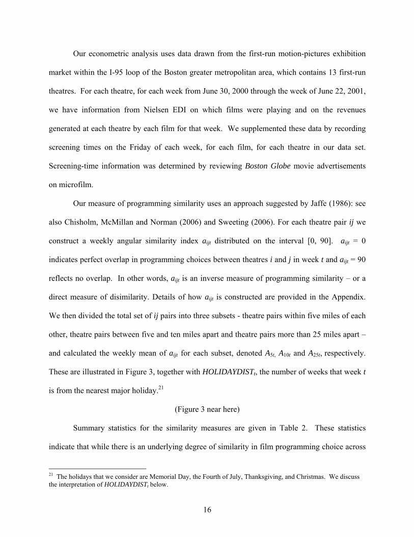
and calculated the weekly mean of aijt for each subset, denoted A5t, A10t and A25t, respectively.

These are illustrated in Figure 3, together with HOLIDAYDISTt, the number of weeks that week t

is from the nearest major holiday.21

(Figure 3 near here)

Summary statistics for the similarity measures are given in Table 2. These statistics

indicate that while there is an underlying degree of similarity in film programming choice across

21 The holidays that we consider are Memorial Day, the Fourth of July, Thanksgiving, and Christmas. We discuss the interpretation of HOLIDAYDISTt below.

17

the theatre pairs in our sample, there is also considerable variability in film programming choice.

The data are also supportive of our hypothesis that programming similarity will decrease (the

angular measure Adt should increase) as substitutability increases. Applying a t-test to compare

the time series for A5t, A10t and A25t, we cannot reject the hypothesis that A5t > A10t and A10t > A25t

at the .01 significance level.

In order to investigate the impact of market size on programming similarity, we construct

two measures of market size. HOLIDAYDISTt, as noted above, is the number of weeks that week

t is from the nearest major holiday. We use HOLIDAYDISTt as an inverse measure of market

size, reflecting the work of Einav (2007), who finds in his analysis of seasonality in movie

theatre revenues that movie audiences build up as we approach major holidays and decline

thereafter. Our second market size measure is AGGREVt, aggregate revenue (in millions of

dollars) in week t of the first-run theatres in our sample. While appealing on its face, there are at

least two reasons for our having reservations in taking AGGREVt as a measure of market size.

First, this is an ex post realization of revenues in week t whereas we would have preferred a

measure of expected revenues. Second, there is the possibility that aggregate revenue overstates

the true seasonality in movie theatre attendance (Einav op. cit.) since the expected boxoffice

appeal and revenue-generating potential of the movies being released is likely to be greater

nearer to major holidays.

We estimate the following reduced form:

(10) dt d d t dtA MARKETSIZEα β ε= + +

where d = 5, 10, 25 and MARKETSIZEt is one of the two proposed measures of market size in

week t (t = 1 …52).

18

Recall that Adt is an inverse measure of similarity, HOLIDAYDISTt is an inverse measure

of market size and AGGREVt is a direct measure of market size. We expect, therefore, that dβ

will be positive (negative) when market size is measured by HOLIDAYDISTt (AGGREVt).

Second, we expect that 5 10 25α α α> > . Returning to Figure 1, we can draw the further inference

that the degree of product line overlap, or programming similarity, is likely to be more sensitive

to market size the lower is the degree of substitutability. In other words, we should expect to

find 25 10 5β β β> > .

The results are summarized in Table 3. With HOLIDAYDISTt as our measure of market

size, the results are consistent with all three hypotheses. With AGGREVt as our measure of

market size, there is some support for the hypothesized relationship between programming

similarity and either market size or substitutability, but not for the hypothesis that programming

similarity is likely to be more sensitive to market size when substitutability is low. This is,

perhaps, a result of the reservations we noted above regarding the use of AGGREVt as a measure

of market size, but is something that should be investigated in more detail in subsequent work,

for example by using Einav’s approach to identify the “true” seasonality in aggregate revenues.

(Table 3 near here)

Some further points are perhaps necessary in support of our suggested interpretation of

these results. It might be suggested that the impact of distance reflects the operation of the

clearance system in film programming, which constrains theatres close to each other from

showing the same films. There are at least two reasons for rejecting this suggestion. First, as

can be seen from Figure 3, there is considerable underlying pair-wise similarity in programming

choice even for theatres that are very close together, which suggests that the clearance system is

not of particular importance. Second, if (di)similarity is driven by the clearance system we

19

would not find the systematic effect of distance on (di)similarity that we do find and that is

predicted by the model.

It might also be argued that the impact of HOLIDAYDISTt and AGGREVt on

programming similarity results from the wide release of major movies at holiday weekends, to

some extent forcing similarity in these weekends, rather than from the impact of market size.

There are at least three reasons for rejecting this interpretation. First, “forced” similarity in

having to carry “blockbusters” can be unwound by the theatre manager in his choice of the other

films to be shown in any given week.22 Second, if there is such a “blockbuster” effect, we would

not find a systematic impact of DISTANCE on similarity, since all theatres would be forced to

carry the same films, no matter their relative locations. Third, if programming similarity were

driven by a “blockbuster” effect rather than the market size effect that we suggest we would not

find the build-up in programming similarity as we approach the holiday weekend “from the

left”.23

7. Concluding Remarks

Will competing multi-product firms choose wide product lines with extensive product

line overlap or narrow product lines with little overlap? We have shown in this paper that the

answer to this question is critically dependent upon the interplay between market size and

product substitutability. This reflects the balance that firms must strike in their choice of product

lines. On the one hand, there are benefits from wider product lines to “be where the demand is”.

22 We are grateful to an industry expert on the movie exhibition market for this argument. 23 There is the further point that if the blockbuster interpretation is to be accepted HOLIDAYRIGHT (a measure of the number of weeks from the most recent past holiday) should dominate HOLIDAYDIST as an explanatory variable - it does not (details can be obtained from the authors on request.) Moreover, Einav’s analysis (op. cit.) identifies a steady build-up in movie-going as we approach major holidays and a decline thereafter, again consistent with our market size interpretation of HOLIDAYDIST and AGGREV.

20

On the other hand, there are costs of wider product lines in tougher competition as a result of

more extensive product line overlap and increased intra-firm product cannibalization.

We have shown that the benefits of broad product lines are more likely to outweigh the

costs in large markets, which favor being where the demand is, or when product substitutability

is low, since this weakens inter-firm competition and intra-firm product cannibalization. In other

words, our analysis yields three testable hypotheses. We should expect to find broader product

lines and more product line overlap in large markets or in markets where product substitutability

is low. We should further expect to find that product line choice is more sensitive to market size

in markets where product substitutability is low.

We have tested these hypotheses and give them broad support, using evidence from film

programming choice in the Boston first-run movie exhibition market.

Our analysis suggests several avenues for further research. The current model imposes

an exogenous maximum degree of product-line expansion on firms, allowing endogenous choice

of product line only within this limit. In addition, we have paid no attention to how a firm

introduces an additional product. This is not unreasonable in the first-run movie exhibition

market where the number of screens at a theatre, which is expensive to change, limits the number

of films that can be shown and where the films themselves are supplied to the theatres by movie

distributors rather than produced “in house”. In other contexts, however, fully endogenizing the

product line decision, and the innovation process by which additional products are brought to

market, would be useful extensions to the product-line rivalry literature.

Second, while our formal model is static, there clearly are interesting dynamic questions

regarding when new products should be introduced and existing products dropped. Some

progress has been made on these questions for the first-run movie exhibition market (Chisholm

21

and Norman, 2006) and for the computer mainframe market (Greenstein and Wade, 1998), but

more extensive analysis, both analytical and empirical, is needed.

22

Figure 1: Subgame Perfect Equilibrium

0 2 4 6 8 100

50

100

150

200

250

300α33u(γ)

α44(γ)

α33l(γ)

α22u(γ)

α22 l(γ)

α11(γ)

α

γ

Figure 2: Critical Discount Factors

0 1 2 3 4 525

50

75

100

125

150

175

α44(γ)

γ

α

d3 = 0d3 = 0.25d3 = 0.5 d2 = 0.25d2 = 0.5

23

Figure 3: Programming Similarity and Distance

0

2

4

6

8

10

12

1 4 7 10 13 16 19 22 25 28 31 34 37 40 43 46 49 52Week

Hol

iday

Dis

tanc

e

0

10

20

30

40

50

60

70

Ang

ular

Sim

ilarit

y

holidaydist A5t A10t A25t

24

Table 1: Equilibrium Quantities and Prices

Product Line Equilibrium Quantities Equilibrium Prices

({1,2,3,4},{1,2,3,4}) 12sVqki =

3Vpi =

({1,2,3,4},{2,3,4}) ( )( )

( )( )γ+

γ+=

γ+γ+

====

3431

342458;

8 4321

sVq

sVqqqsVq

Bi

AAAA

( )

3

;34

2

432

1

Vppp

Vp

===

γ+γ+

=

({1,2,3,4},{3,4}) ( )( )

( )( )λ+

γ+==

γ+γ+

====

261

2244;

8

43

4321

sVqq

sVqqsVqq

BB

AAAA

( )( )

3

233

43

21

Vpp

Vpp

==

γ+γ+

==

({1,2,3,4},{4}) ( )( )

( )( )λ+

γ+=

γ+γ−

====

431

4248;

8

4

4321

sVq

sVqsVqqq

B

AAAA

( )( )

3

436

4

321

Vp

Vppp

=

γ+γ+

===

({1,2,3},{2,3,4}) ( )

( )( )γ+

γ+====

γ+γ+

==

78312

;78

1

3232

41

sVqqqq

sVqq

BBAA

BA

( )( )

3

;783712

32

41

Vpp

Vpp

==

γ+γ+

==

({1,2,3},{3,4}) ( )( )( )

( )( )( )

( )( )( )

( )( )24

2323

221

114032212

1140323581;

1140323412

;1140322

381

γ+γ+γ+γ+

=

γ+γ+γ+γ+

=γ+γ+γ+γ+

=

γ+γ+γ+γ+

==

sVq

sVqsVq

sVqq

B

BA

AA

( )( )

( )( )2

2

4

3

2

2

21

1140323114448

;3

;1140323115048

γ+γ+γ+γ+

=

=

γ+γ+γ+γ+

==

Vp

Vp

Vpp

({1,2,3},{4}) ( )( )

( )( )24

2321

96464381

;96464

341

γ+γ+γ+γ+

=

γ+γ+γ+γ+

===

sVq

sVqqq

B

AAA

( )( )

( )( )24

2321

96464384

;96464348

γ+γ+γ+γ+

=

γ+γ+γ+γ+

===

Vp

Vppp

({1,2},{3,4}) ( )( )γ+

γ+=

3421sVqki ( )

γ+γ+

=34

2Vpi

({1,2},{4}) ( )( )( )

( )( )( )24

221

66331

;666

61

γ+γ+γ+γ+

=

γ+γ+γ+γ+

==

sVq

sVqq

B

AA

( )( )( )

( )( )2

2

4

221

6633

;666

236

γ+γ+γ+

=

γ+γ+γ+γ+

==

Vp

Vpp

({1},{4}) ( )γ+γ+

==34

141

sVqq BA ( )γ+γ+

==34

241

Vpp

25

Table 2: Summary Statistics for Average Angular Similarity Index by Distance

Similarity Measure

At A5t A10t A25t

Mean 39.74 50.06 44.94 33.23

Variance 21.64 19.56 18.39 31.00

Minimum 30.61 39.72 37.30 22.28

Maximum 50.72 60.85 56.45 43.71

Adt is the average weekly angular measure of similarity for theatre pairs by distance between theatres over 52 weeks: A5t for less than five miles; A10t between 5 and 10 miles; A25t over 25 miles; At across all theatre pairs.

Table 3: Estimation of Average Angular Similarity Index by Distance

Variable At A5t A10t A25t

HOLIDAYDISTt 1.005

(0.149)***

0.722

(0.180)***

0.864

(0.155)***

1.182

(0.163)***

CONSTANT 35.39

(0.808)***

46.94

(0.948)***

41.20

(0.677)***

28.12

(0.971)***

R2 0.454 0.259 0.394 0.438

F Value 45.21 16.14 31.16 52.43

Variable At A5t A10t A25t

AGGREVt -4.464

(1.308)***

-0.914

(1.433)

-5.539

(1.184)***

-4.782

(1.481)**

CONSTANT 45.44

(1.902)***

51.23

(2.161)***

52.02

(1.760)***

39.35

(2.120)***

R2 0.170 0.008 0.308 0.136

F Value 11.64 0.526 21.89 10.42 Estimation by OLS with robust standard errors. Dependent variable is Adt is the average weekly angular measure of similarity for theatre pairs by distance between theatres: A5t for less than five miles; A10t between 5 and 10 miles; A25t over 25 miles; At across all theatre pairs. Sample size is 52. Significance levels *.10, **.05, ***.01; standard errors reported in parentheses.

26

References Anderson, Simon P. and Neven, Damien. 1991. “Cournot Competition Yields Spatial

Agglomeration,” International Economic Review, Volume 32, pp. 767-782 Anderson, Simon P. and De Palma, André. 2006. “Market Performance with Multiproduct

Firms,” Journal of Industrial Economics, Volume LIV, pp. 95-124. Bernheim, B. Douglas and Whinston, Michael D. 1990. “Multimarket Contact and Collusive

Behavior,” RAND Journal of Economics, Volume 21, pp. 1-21. Brander, James A. and Eaton, Jonathan. 1984. “Product Line Rivalry,” American Economic

Review, Volume 74, pp. 323-334. Busse, Meghan R. 2000. “Multimarket Contact and Price Coordination in the Cellular Telephone

Industry,” Journal of Economics and Management Strategy, Volume 9, pp. 287-320. Chisholm, Darlene C. and Norman, George. 2006. “When to Exit a Product: Evidence from the

U.S. Motion Picture Exhibition Market,” American Economic Review, Papers and Proceedings, Volume 96, no. 2, pp. 57-61.

Chisholm, Darlene C., McMillan, Margaret S. And Norman, George. 2006. “Product

Differentiation and Film Programming Choice: Do First-Run Movie Theatres Show the Same Films?” N.B.E.R. Working Paper No. 12646, Cambridge, Mass.

d’Aspremont, Claude, Gabszewicz, Jean J. and Thisse, Jacques-Francois. 1979. “On Hotelling’s

‘Stability in Competition,’” Econometrica, Volume 47, pp. 1145-50. De Fraja, Giovanni. 1996. “Product Line Competition in Vertically Differentiated Markets,”

International Journal of Industrial Organization, Volume 14, pp. 389-414. Dixit, Avinash and Stiglitz, Joseph E. 1977. “Monopolistic Competition and Optimal Product

Diversity,” American Economic Review, Volume 69, pp. 297-308. Dobson, Paul and Waterson, Michael. 1996. “Product Range and Interfirm Competition,”

Journal of Economics and Management Strategy, Volume 35, pp. 317-341. Draganska, Michaela and Jain, Dipak C. 2005. “Product Line Length and a Competitive Tool,”

Journal of Economics and Management Strategy, Volume 14, pp. 1-29. Eaton, B. Curtis and Lipsey, Richard G. 1979. “The Theory of Market Pre-Emption: the

persistence of excess capacity and monopoly in growing spatial markets,” Economica, Volume 46, pp. 149-158.

Eaton, B. Curtis and Schmitt, Nicolas. 1994. “Flexible Manufacturing and Market Structure,”

American Economic Review, Volume 84, pp. 875-888.

27

Einav, Liran. 2007. “Seasonality in the U.S. Motion Picture Industry,” RAND Journal of

Economics, forthcoming. Feinberg, Robert M. 2003. “The Determinants of Bank Rates in Local Consumer Lending

Markets: Comparing Market and Institution-Level Results,” Southern Economic Journal, Volume 70, pp. 144-156.

Greenstein, Shane M. and Wade, James B. “The Product Life Cycle in the Commercial

Mainframe Computer Market, 1968-1982,” RAND Journal of Economics, Winter 1998, 29(4), pp. 772-89.

Gupta, Srabana. 2001. “The Effect of Bid Rigging on Prices: A Study of the Highway

Construction Industry,” Review of Industrial Organization, Volume 19, pp. 453-467. Hotelling, Harold. 1929. “Stability in Competition,” Economic Journal, Volume 39, pp. 41-57. Jaffe, Adam B. 1986. “Technological Opportunity and Spillovers of R&D: Evidence from

Firms’ Patents, Profits, and Market Value,” American Economic Review, Volume 76, pp. 984-1001.

Klemperer, Paul. 1992. “Equilibrium Product Lines: competing head-to-head may be less

competitive,” American Economic Review, Volume 82, pp. 741-755. Lal, Rajiv and Matutes, Carmen. 1989. “Price Competition in Multiproduct Duopolies,” RAND

Journal of Economics, Volume 20, pp. 516-537. Manez, Juan A. and Waterson, Michael. 2001. “Multiproduct Firms and Product Differentiation:

a survey,” Warwick Economic Research Papers No. 594, University of Warwick. Motta, Massimo. 2004. Competition Policy: Theory and Practice, Cambridge, Cambridge

University Press. Phlips, Louis. 1983. The Economics of Price Discrimination, Cambridge, Cambridge University

Press. Schmalensee, Richard. 1978. “Entry Deterrence in the Ready-To-Eat Breakfast Cereal Industry,”

Bell Journal of Economics, Volume 9, pp. 305-327. Shaked, Avner and Sutton, John. 1990. “Multiproduct Firms and Market Structure,” RAND

Journal of Economics, Volume 21, pp. 45-62. Shubik, Martin and Levitan, Richard. 1980. Market Structure and Behavior, Cambridge Mass.,

Harvard University Press.

28

Spence, Michael. 1976. “Product Selection, Fixed Costs and Monopolistic Competition,” Review of Economic Studies, Volume 43, pp. 217-235.

Sweeting, Andrew. 2006. “Too Much Rock and Roll? Station Ownership, Programming and

Listenership in the Music Radio Industry,” Northwestern University Working Paper. Tirole, Jean. 1988. The Theory of Industrial Organization, The MIT Press, Cambridge,

Massachusetts.

29

Appendix: Angular Similarity Index

Following Jaffe (1986), Chisholm, Norman and McMillan (2006), and Sweeting (2006),

suppose that there are Mt different movies being shown in week t in our population of first-run

movie theatres. Order these movies alphabetically and define mt as the mth movie being shown

(in at least one of the theatres) in week t. Then we can create the Mt x 1 vector

( )iMimiiit ttttppppp ,..,,..,, 21= for theatre i, where imt

p is the percentage of show-times at theatre

i devoted to film mt in week t.24

Given the vectors pit and pjt for theatres i and j we define the angular similarity index aijt for

this theatre pair as the angle between these two vectors:

⎟⎟

⎠

⎞

⎜⎜

⎝

⎛ ⋅=

jtit

jtitijt pp

ppa arccos .

An important characteristic of this angular similarity index is that the “measure of proximity

is purely directional i.e. it is not directly affected by the length of the (p) vectors.” (Jaffe, 1986,

p. 986, fn 5)

24 In the empirical application we measure show-times on the Friday of each week.