Aalto UniversitySchool of ScienceDegree programme in Engineering Physics and Mathematics

Production Planning of a Pumped-storage

Hydropower Plant

MS-E2108 Independent research projects in systems analysis8.9.2015

Eero Lehtonen

Advisor: Dr. Anssi Käki, UPMSupervisor: Prof. Ahti Salo

The document can be stored and made available to the public on the openinternet pages of Aalto University.All other rights are reserved.

Contents

1 Introduction 1

2 Background 1

2.1 Hydropower . . . . . . . . . . . . . . . . . . . . . . . . . . . . 22.2 Electricity Markets . . . . . . . . . . . . . . . . . . . . . . . . 32.3 Pricing of Water . . . . . . . . . . . . . . . . . . . . . . . . . 32.4 Pumped-storage Hydropower . . . . . . . . . . . . . . . . . . . 42.5 Planning Hydroelectric Production . . . . . . . . . . . . . . . 5

3 Production Planning Model 7

3.1 Notation . . . . . . . . . . . . . . . . . . . . . . . . . . . . . . 83.2 Objective Function . . . . . . . . . . . . . . . . . . . . . . . . 93.3 Hydrobalance . . . . . . . . . . . . . . . . . . . . . . . . . . . 93.4 Environmental Limits . . . . . . . . . . . . . . . . . . . . . . . 103.5 Q-E Pro�les and Operating Modes . . . . . . . . . . . . . . . 103.6 Mode Switching Costs and Delays . . . . . . . . . . . . . . . . 123.7 Frequency Controlled Reserves . . . . . . . . . . . . . . . . . . 133.8 Traditional Turbine Operation . . . . . . . . . . . . . . . . . . 153.9 Summarized MILP problem . . . . . . . . . . . . . . . . . . . 153.10 Rolling Optimization . . . . . . . . . . . . . . . . . . . . . . . 15

4 Results and Discussion 16

1 Introduction

This study describes the production planning of a hydropower plant operat-ing in the deregulated Nordic electricity market. The project was initiated bya Finnish energy company to evaluate possible bene�ts of a pumped-storagehydro plant over a conventional hydropower plant. Planning was performedfor both a conventional hydropower plant and a pumped-storage hydropowerplant under the same market and environmental circumstances in order toevaluate the economical feasibility of pumped-storage under such conditions.

The problem was modeled as an iterative mixed integer programming (MILP)problem that aims to maximize total revenue gained over a given times-pan. Hydropower production planning has been studied before: Conejo et al.[2002] describe a similar multi-plant production planning problem in a pool-based electricity market. Pursimo et al. [1998] also describe an optimal con-trol approach to planning the production of a chain of hydro plants in theriver Kemijoki. Wallace and Fleten [2003] also discuss a hydro unit com-mitment problem under uncertainty from a cost-minimization perspective.The model presented in this study considers a single plant in a deterministicsetting. More importantly, in order to re�ect the operation of a pumped-storage plant, the model extends conventional hydropower modeling to allowthe plant to pump water into its upper reservoir. The model also accountsfor start-up and switching costs.

The model was implemented using AMPL and the CPLEX solver. The modelwas used to compute revenue-maximizing hourly production amounts for apumping plant and a conventional hydroplant the years 2013 and 2014. Thecase company provided input data that was used in the production planningprocess.

The rest of this study is structured as follows: the relevant principles ofhydropower and deregulated energy markets are discussed in Section 2. Theproduction planning model formulation is presented in Section 3. Finallyresults from the production planning process are summarized in Section 4.

2 Background

In this section, the fundamentals of hydropower production planning are dis-cussed. First the central principles of hydroelectric power generation arediscussed in Section 2.1. Then, both the international Nord Pool Spot and

2

domestic balancing power markets are brie�y introduced in Section 2.2. Ap-proaches to pricing reservoir water are discussed in Section 2.3 and additionalconsiderations related to pumped-storage hydropower are reviewed in Sec-tion 2.4. Finally issues in production planning of hydroelectric production isdiscussed in Section 2.5.

2.1 Hydropower

Hydropower is generated from the potential energy of falling water. A hy-dropower plant generates electrical power from falling water using a turbineand a generator. Water rotates the turbine through which it �ows and thegenerator produces electrical energy using the rotational motion of the tur-bine.

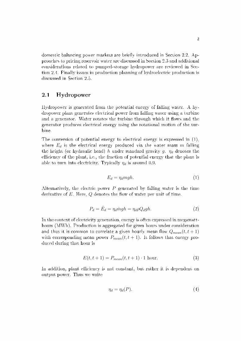
The conversion of potential energy to electrical energy is expressed in (1),where Ed is the electrical energy produced via the water mass m fallingthe height (or hydraulic head) h under standard gravity g. ηd denotes thee�ciency of the plant, i.e., the fraction of potential energy that the plant isable to turn into electricity. Typically ηd is around 0.9.

Ed = ηdmgh. (1)

Alternatively, the electric power P generated by falling water is the timederivative of E. Here, Q denotes the �ow of water per unit of time.

Pd = Ed = ηdmgh = ηdρQdgh. (2)

In the context of electricity generation, energy is often expressed in megawatt-hours (MWh). Production is aggregated for given hours under considerationand thus it is common to correlate a given hourly mean �ow Qmean(t, t+ 1)with corresponding mean power Pmean(t, t + 1). It follows that energy pro-duced during that hour is

E(t, t+ 1) = Pmean(t, t+ 1) · 1 hour. (3)

In addition, plant e�ciency is not constant, but rather it is dependent onoutput power. Thus we write

ηd = ηd(P ). (4)

3

For convenience, a mean �ow to energy curve (from here on referred to asthe Q-P or Q-E curve) is estimated. For a single generator plant this curveis assumed to be concave, i.e., the e�ciency curve reaches a global maximumat some optimal P and decreases when deviating further from optimal oper-ation. Hence P (Q) and E(Q) are concave, which simpli�es their inclusion inthe optimization model.

2.2 Electricity Markets

Most of electricity produced in the Nordic countries is sold to the day-aheadmarket of Nord Pool Spot [2014]. A market clearing spot price for each houris computed from production and consumption bids submitted by partici-pants. The market is divided into areas, in which prices may deviate froma market-wide system price due to limited inter-area transfer capacity. Formore information, see Nord Pool Spot [2015].

In addition to the Nord Pool Spot markets, the Finnish transmission systemoperator (TSO) Fingrid conducts balance management between productionand consumption via intra-day balancing power markets. Power balance ismanaged via two markets: the balancing power market, where producingand consuming participants are o�ered respectively a premium or discountto the corresponding spot price for adjusting their original contribution, andthe frequency-controlled reserves (FCR) market, where participants sell re-serve capacity that can be automatically adjusted when frequency in the griddeviates from a speci�ed range.

In this assignment only the Elspot and FCR markets were considered, be-cause they are the only relevant sources of revenue for the plant in question.Also, accounting for other markets, such as the balancing power market,would require modeling of uncertainties related to the balancing demandand price.

2.3 Pricing of Water

In thermal energy production, the produced energy is priced according tomarginal cost, i.e., the cost of producing an additional unit of energy. As-suming perfectly competitive markets and a strictly increasing marginal costcurve, such pricing maximizes pro�ts, because marginal cost below sale pricewould indicate the existence of untapped pro�ts and marginal cost above

4

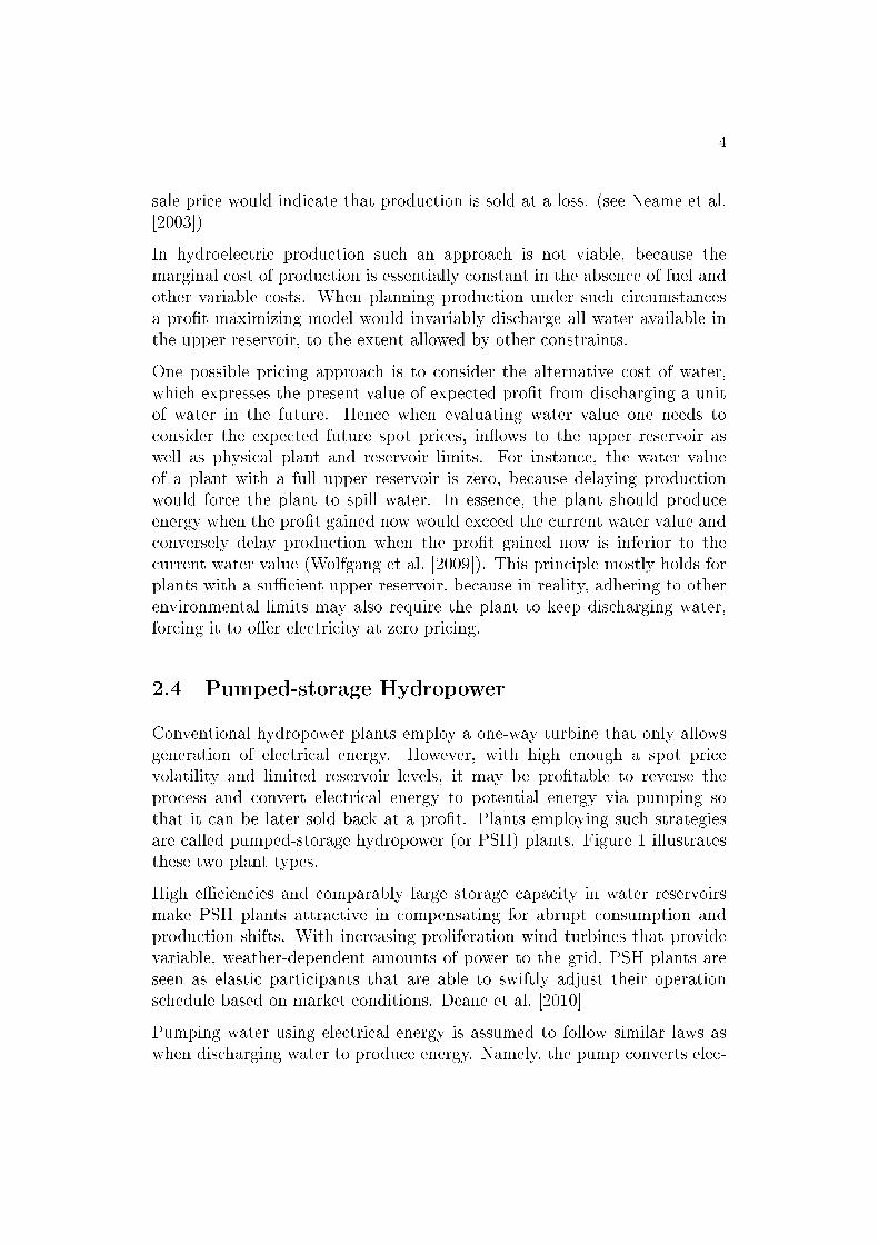
sale price would indicate that production is sold at a loss. (see Neame et al.[2003])

In hydroelectric production such an approach is not viable, because themarginal cost of production is essentially constant in the absence of fuel andother variable costs. When planning production under such circumstancesa pro�t maximizing model would invariably discharge all water available inthe upper reservoir, to the extent allowed by other constraints.

One possible pricing approach is to consider the alternative cost of water,which expresses the present value of expected pro�t from discharging a unitof water in the future. Hence when evaluating water value one needs toconsider the expected future spot prices, in�ows to the upper reservoir aswell as physical plant and reservoir limits. For instance, the water valueof a plant with a full upper reservoir is zero, because delaying productionwould force the plant to spill water. In essence, the plant should produceenergy when the pro�t gained now would exceed the current water value andconversely delay production when the pro�t gained now is inferior to thecurrent water value (Wolfgang et al. [2009]). This principle mostly holds forplants with a su�cient upper reservoir, because in reality, adhering to otherenvironmental limits may also require the plant to keep discharging water,forcing it to o�er electricity at zero pricing.

2.4 Pumped-storage Hydropower

Conventional hydropower plants employ a one-way turbine that only allowsgeneration of electrical energy. However, with high enough a spot pricevolatility and limited reservoir levels, it may be pro�table to reverse theprocess and convert electrical energy to potential energy via pumping sothat it can be later sold back at a pro�t. Plants employing such strategiesare called pumped-storage hydropower (or PSH) plants. Figure 1 illustratesthese two plant types.

High e�ciencies and comparably large storage capacity in water reservoirsmake PSH plants attractive in compensating for abrupt consumption andproduction shifts. With increasing proliferation wind turbines that providevariable, weather-dependent amounts of power to the grid, PSH plants areseen as elastic participants that are able to swiftly adjust their operationschedule based on market conditions. Deane et al. [2010]

Pumping water using electrical energy is assumed to follow similar laws aswhen discharging water to produce energy. Namely, the pump converts elec-

5

Figure 1: A diagram of a PSH plant. The turbine is used to both generateelectricity via discharging water from the reservoir and to pump water to thereservoir by consuming electricity.

trical energy into potential energy with e�ciency ηp ∈ ]0, 1[:

mgh = ηpEp.

As with ηd, ηp is also assumed to be power-dependent with similar properties.The round-trip e�ciency is an e�ciency measure for a PSH plant de�nedas the fraction of energy produced via discharge of a water unit and thecorresponding electrical energy consumed to pump a unit of water into thereservoir:

ηroundtrip =EdEp

= ηdηp

In addition, it should be noted that also the production e�ciency nd is smallerfor a pumping turbine when compared to conventional hydropower turbines.In essence, the pumping turbine, if used only for production, would operateat an economical loss compared to a conventional turbine.

2.5 Planning Hydroelectric Production

In this assignment a simple hydroelectric plant with a small, regulated upperreservoir and an e�ectively unlimited lower reservoir is considered. The �owsinto the upper reservoir are given. A simple �ow diagram of the reservoir and�ows is shown in Figure 2. At a given hour t, V t denotes the upper reservoirvolume, Qt

in denotes �ows beside those from the plant into the reservoir, Qtd

6

denotes discharges through the plant, Qtp denotes pumping �ows into the

reservoir and W t denotes �ows from spilling.

Qtin

Qtd Qt

p W t

V t

Figure 2: Flow Diagram

The plant is scheduled so as to maximize revenue under physical operationallimits of the plant as well as limits posed by the upper reservoir.

A substantial issue in planning hydroelectric production is to evaluate resid-ual value of water in the end of the planning period so as to prevent themodel from discharging all available water by the end of the planning pe-riod. Ideally one would add the water value of the water remaining in thereservoir after the planning period to the objective function. However, com-puting water value even for a simple system of a single plant and reservoir isdi�cult, and several proxies and alternative approaches can be used to limitdischarge when planning hydroelectric production. Førsund [2007] amongothers discuss such methods including the ones discussed below.

Rudimentary water value estimation One can estimate water value bymultiplying the terminal reservoir level with a coe�cient ρ < 1. Thiscoe�cient should re�ect the possibility of the reservoir �lling up andthus reducing the unit value of water as well as other limits forcing theplant to run ine�ciently.

Fixed terminal reservoir The plan may be constrained to reach a �xedterminal reservoir level Vf . The terminal reservoir level should againre�ect the alternative cost of water.

Increased optimization period The model may be optimized far in to thefuture so that only a small period in the beginning of the optimizationperiod is used as a production plan. With a long enough optimizationhorizon, the terminal discharge e�ect should be mitigated within thebeginning of the period.

7

In this project, a combination of the second and third methods was used. Theplanning interval was split into successive, partially overlapping subintervalsand the plan was optimized for each subinterval so that the initial conditionswere taken from the previous subinterval and the terminal reservoir level wasconstrained to a sensible level. Consequently, the aggregate plan was allowedto deviate from the constrained reservoir levels within each subinterval tothe extent that the reservoir could be steered to the required terminal levelduring that interval. The rolling optimization method is further explainedin Section 3.10.

3 Production Planning Model

The production planning problem is modeled as a mixed integer linear pro-gramming (MILP) problem that maximizes forecasted pro�ts from the spotand frequency markets. Constraints are introduced in order to respect phys-ical limitations, �ow-power relationships, as well as switching between pro-duction, pumping and o�-line modes. The constraints are grouped as follows:

Hydrobalance Reservoir level is determined by in�ows and discharges.

Environmental regulations The plant needs to respect reservoir level reg-ulations.

Plant operating ranges The plant variables need to remain within speci-�ed domains.

Flow-power mapping Piecewise-linear discharge-to-power and power-to-in�ow mappings are modeled as constraints.

Mode switching Operating mode switching is tracked via binary constraintson operating modes.

Frequency Reserves The plant can reserve capacity to the frequency re-serve markets during running hours.

Due to the hourly resolution of physical electricity markets, it is reasonableto model the production planning problem in an hourly resolution as well. Inthe following de�nitions, all references to time refer to hours and all quantitiesare treated as hourly means.

8

3.1 Notation

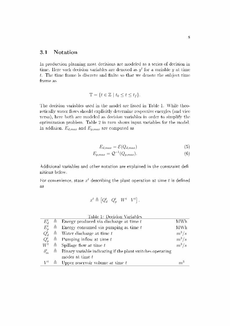
In production planning most decisions are modeled as a series of decision intime. Here such decision variables are denoted as yt for a variable y at timet. The time frame is discrete and �nite so that we denote the subject timeframe as

T = {t ∈ Z | t0 ≤ t ≤ tf}.

The decision variables used in the model are listed in Table 1. While theo-retically water �ows should explicitly determine respective energies (and viceversa), here both are modeled as decision variables in order to simplify theoptimization problem. Table 2 in turn shows input variables for the model.In addition, Ed,max and Ep,max are computed as

Ed,max = E(Qd,max) (5)

Ep,max = Q−1(Qp,max). (6)

Additional variables and other notation are explained in the constraint de�-nitions below.

For convenience, state xt describing the plant operation at time t is de�nedas

xt ,[Qtd Qt

p W t V t].

Table 1: Decision VariablesEtd , Energy produced via discharge at time t MWh

Etp , Energy consumed via pumping at time t MWh

Qtd , Water discharge at time t m3/s

Qtp , Pumping in�ow at time t m3/s

W t , Spillage �ow at time t m3/s

δtm , Binary variable indicating if the plant switches operatingmodes at time t

V t , Upper reservoir volume at time t m3

9

Table 2: Input Variablesptf , Forecasted spot price at time t. ept , Realized spot price at time t. ePm , A �xed cost associated with switching operating modes. e

PFCR−D , Yearly market price of frequency controlled disturbancereserves

e

PFCR−N , Yearly market price of frequency controlled normal op-eration reserves

e

V tl , Minimum upper reservoir volume at time t m3

V tu , Maximum upper reservoir volume at time t m3

Qtin , Upper reservoir in�ow at time t m3/s

Qd,max , The maximum discharge �ow m3/s

Qp,max , The maximum pump �ow m3/s

3.2 Objective Function

The objective function to be maximized is the total revenue gained from boththe spot and the frequency controlled reserves market less the cost incurredfrom switching operating modes.

∑t∈T

ptf · (Etd − Et

p)− δtmPm +∑t∈T

[CtFCR−DPFCR−D + Ct

FCR−NPFCR−N ] (7)

3.3 Hydrobalance

In hydroplanning, all water �ows should be accounted for and water shouldnot vanish nor appear into the reservoir outside the accounted in�ows anddischarges. This requirement is modeled as the following constraint:

V t = V t−1 + 3600 · (Qt−1in −Qt−1

d +Qt−1p −W t−1) ∀t ∈ (t0 + 1) . . . tf , (8)

where the coe�cient 3600 is used to convert �ows in m3/s to volumes in anhour m3.

The initial and �nal reservoir levels are given as inputs to the model as V0and Vf respectively,

10

V t0 = V0 (9)

V tf = Vf . (10)

3.4 Environmental Limits

Regulated reservoirs have time dependent upper and lower limits for waterlevel changes due to spring �oods and preservation of biodiversity in the vicin-ity of the reservoir. Here these limits are accounted for with correspondingreservoir volumes.

V tl ≤ V t ≤ V t

u ∀t ∈ T. (11)

The plant also has hard limits on its spillage capacity.

Wl ≤ W t ≤ Wu ∀t ∈ T. (12)

3.5 Q-E Pro�les and Operating Modes

The discharge-to-output-power mapping is modeled as a concave, piecewise-linear function here denoted as E(Q). Such a �t for measured discharge andoutput power values is shown in Figure 3. Figure 4 shows the correspondinge�ciency curve. As required, the Q-E-curve is concave and the e�ciencycurve has a unique maximum, decreasing steeply to its left and more gradu-ally to its right. It is also assumed that the pump has a similar operationale�ciency pro�le and hence the input-power-to-�ow pro�le Q(E) is modeledas a similar concave, piecewise-linear function. Binary indicators "is dis-charging" and "is pumping" are introduced in order to indicate if the plantis discharging or pumping water at any given hour. M denotes a large posi-tive constant. The constraint (17) forces the model to discharge water, pumpwater or to stay idle. These indicators are later related to mode switchingcosts and delays as well as FCR bidding opportunities.

Etd ≤ E(Qt

d) +M · (1− δtd) ∀t ∈ T (13)

Etd ≤M · δtd ∀t ∈ T (14)

11

Figure 3: Piecewise-linear Q-E-curve �tted against measured discharge andpower output.

Qtp ≤ Q(Et

p) +M · (1− δtp) ∀t ∈ T (15)

Qtp ≤M · δtp ∀t ∈ T (16)

δtd + δtp ≤ 1 ∀t ∈ T (17)

In addition, hard �ow limits and mode indicators are combined into con-straints forcing both discharge and pump �ows to within hard limits duringoperation and to zero during o�-line hours.

δtd ·Ql ≤ Qtd ≤ δtd ·Qu ∀t ∈ T (18)

δtp ·Ql ≤ Qtp ≤ δtp ·Qu ∀t ∈ T (19)

12

Figure 4: Theoretical e�ciency curve corresponding to the piecewise-linearQ-E-curve in Figure 3

3.6 Mode Switching Costs and Delays

A �xed cost Pm is associated with starting either the pump or the turbine.The binary decision variables δtm in the objective function account for eachmode change and the following constraints are introduced to force the vari-able to one each time the plant switches modes. The binary variables δtd,↑and δtp,↑ are used to indicate if either the turbine or pump is started at hourt.

δtd,↑ ≥ δtd − δt−1d ∀t ∈ T (20)

δtp,↑ ≥ δtp − δt−1p ∀t ∈ T (21)

δtm ≥ δtd,↑ ∀t ∈ T (22)

δtm ≥ δtp,↑ ∀t ∈ T (23)

In addition to mode switching costs, the model also accounts for ramp-upand ramp-down delays as reduced maximum discharge and pump �ows for

13

hours when either mode is switched on or o�. It is assumed that the plantcould linearly ramp up to or down from the maximum capacity Qu in tswitchminutes. The modeled mode switch delay is de�ned in (24). The de�nitionviolates linearity due to multiplication of decision variables and is thereforenot suitable as a constraint in the MILP model. The constraints in (25) - (27)force the corresponding decision variables to take values according to (24).Equivalent non-linear equality constraints and substituted linear inequalityconstraints are introduced for discharge stops as well as pump starts andstops,

Qtstart,d = δtd,↑ ·Qt

d · tswitch/60/2 ∀t ∈ T. (24)

Qtstart,d ≤M · δtd,↑ ∀t ∈ T (25)

Qtstart,d ≤ Qt

d · tswitch/60/2 ∀t ∈ T (26)

Qtstart,d ≥ Qt

d · tswitch/60/2−M · δtd,↑ ∀t ∈ T (27)

Using the mode switch delays de�ned above e�ective upper limits for Qtd and

Qtp are de�ned as the hard upper limit Qu less delay losses due to either

starting or stopping.

Qtd ≤ Qu −Qt

start,d −Qtstop,d ∀t ∈ T (28)

Qtp ≤ Qu −Qt

start,p −Qtstop,p ∀t ∈ T (29)

3.7 Frequency Controlled Reserves

The plant may also participate in the frequency controlled reserves market.Reserve capacity may be sold to the frequency controlled disturbance reserves(FCR-D) and to the frequency controlled normal operation reserves (FCR-N).Selling to these reserves does not incur �ows but large production amountslimit the amount of headroom, i.e., the unused capacity available for usein the FCR, that can be sold to either reserve. According to Fin [2015,Appendix 2], the capacity sold to normal operation reserves needs to beadjustable in both directions, i.e., during discharge hours the plant needs tobe able to both increase and decrease production, and during pumping hoursthe plant needs to be able to both increase and decrease consumption by the

14

sold reserve capacity. Selling capacity to the disturbance reserves in turnonly obliges the plant to be able to increase its production or decrease itsconsumption by the set amount.

Due to rapid shifts required from FCR capacity it is also assumed that theplant needs to be on-line for all hours sold to the FCR market as well as thatthe plant may not switch modes to accommodate frequency correction.

To determine available capacities for a given hour t four auxiliary variablesare introduced. Ct

d,↑ and Ctd,↓ indicate the headroom available in either di-

rection during discharge hours. Ctp,↑ and Ct

p,↓ indicate the same quantitiesfor pumping hours, i.e.,

Ctd,↑ ≤ δtd ·M ∀t ∈ T (30)

Ctd,↑ ≤ Ed,max − Et

d ∀t ∈ T (31)

Ctd,↓ ≤ δtd ·M ∀t ∈ T (32)

Ctd,↓ ≤ Et

d ∀t ∈ T (33)

Ctp,↑ ≤ δtp ·M ∀t ∈ T (34)

Ctp,↑ ≤ Ep,max − Et

p ∀t ∈ T (35)

Ctp,↓ ≤ δtp ·M ∀t ∈ T (36)

Ctp,↓ ≤ Et

p ∀t ∈ T. (37)

Here Ed,max = E(Qu) and Ep,max = Q−1(Qu) withQ−1 denoting the inverse ofQ. In essence, the quantities indicate the maximum energy output producedvia discharge and maximum energy input consumed by pumping respectively.

With these auxiliary headroom variables de�ned, the FCR capacity con-straints are de�ned as follows. It is assumed that the plant has a limitedcapacity that can be sold to the FCR markets at any given time.

CtFCR−N ≤ CFCR−N,max (38)

CtFCR−D ≤ CFCR−D,max. (39)

The headroom variables are then used to limit the hourly FCR capacity salesaccording to limits described above. The Big M Method is used here to targeteither discharge or pump capacity accordingly.

15

CtFCR−D ≤ Ct

d,↑ +M · δtp ∀t ∈ T (40)

CtFCR−D ≤ Ct

d,↓ +M · δtp ∀t ∈ T (41)

CtFCR−D ≤ Ct

p,↑ +M · δtd ∀t ∈ T (42)

CtFCR−D ≤ Ct

p,↓ +M · δtd ∀t ∈ T (43)

CtFCR−N ≤ Ct

d,↑ − CtFCR−D +M · δtp ∀t ∈ T (44)

CtFCR−N ≤ Ct

p,↓ − CtFCR−D +M · δtd ∀t ∈ T (45)

3.8 Traditional Turbine Operation

For comparison purposes the same model can be used to �nd optimal produc-tion plans for a plant without a pump. To facilitate this a simple additionalconstraint is added to disallow pumping,

δtp = 0 ∀t ∈ T. (46)

Additionally, as mentioned in 2.4, it is typical that the Q-E curve E needs tobe re-evaluated for the traditional turbine, too.

3.9 Summarized MILP problem

With objective function and constraints de�ned above, the MILP problemcan be now expressed in a summarized form:

maximizeQd,Qp,W

(7)

subject to (8)− (45)(47)

3.10 Rolling Optimization

In order to force the model to maintain sensible water levels in the longterm, the production planning problem is split into partially overlapping

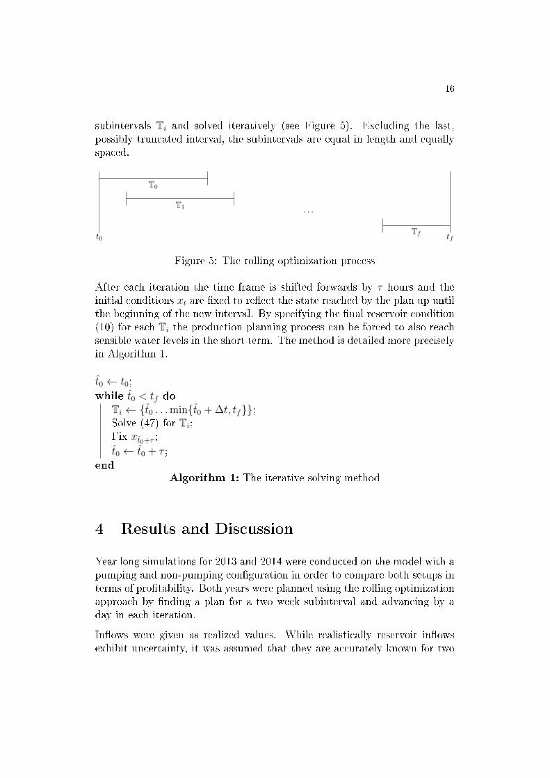
16

subintervals Ti and solved iteratively (see Figure 5). Excluding the last,possibly truncated interval, the subintervals are equal in length and equallyspaced.

t0 tf

. . .

T0

T1

Tf

Figure 5: The rolling optimization process

After each iteration the time frame is shifted forwards by τ hours and theinitial conditions xt are �xed to re�ect the state reached by the plan up untilthe beginning of the new interval. By specifying the �nal reservoir condition(10) for each Ti the production planning process can be forced to also reachsensible water levels in the short term. The method is detailed more preciselyin Algorithm 1.

t0 ← t0;

while t0 < tf doTi ← {t0 . . .min{t0 + ∆t, tf}};Solve (47) for Ti;Fix xt0+τ ;

t0 ← t0 + τ ;

endAlgorithm 1: The iterative solving method

4 Results and Discussion

Year long simulations for 2013 and 2014 were conducted on the model with apumping and non-pumping con�guration in order to compare both setups interms of pro�tability. Both years were planned using the rolling optimizationapproach by �nding a plan for a two week subinterval and advancing by aday in each iteration.

In�ows were given as realized values. While realistically reservoir in�owsexhibit uncertainty, it was assumed that they are accurately known for two

17

Figure 6: A model generated schedule for 6.5.2013 - 12.5.2013. The planttargets high spot prices for production hours and low prices for consumptionhours.

weeks in advance. Revenue was maximized against forecasted spot prices but�nally also compared to realized spot prices.

Years with di�erent fundamental properties were selected in order to com-pare the PSH plant's relative performance under di�erent circumstances.The selected years exhibit di�erences in spot prices as well as in�ow levels.In 2013, there was approximately 21% less natural in�ow and approximately14% higher spot prices in comparison to 2014. It was hypothesized that thePSH plant might perform relatively better during dry years when dischargecapacity is not saturated for long periods of time. This hypothesis was val-idated by the production planning process: in 2013 the PSH plan pumped12.8% more water in comparison to the plan computed for 2014. However,the qualitative results for both years were altogether similar, and hence the�gures and discussion below focus on the year 2013.

Figure 6 shows a week long example of the model-generated PSH plan againstrealized spot prices. The plan targets high-priced hours for production andlow-priced hours for consumption. FCR capacity is traded for expandedproduction or consumption only during the most expensive or cheap hoursrespectively. This is expected, because the additional pro�t or reduction in

18

Figure 7: Mean discharge �ows for the conventional and PSH plants in 2013.Pumping and corresponding additional discharge by the PSH plant are sched-uled from April to July and September to December.

cost obtained during full operation needs to outweigh the alternative costof shifting that production to hours with more headroom and a lower price.In the week long period the plant consistently runs when the spot price ishigher than approximately 40 e/MWh and pumps when the price is lowerthan approximately 30 e/MWh.

In addition, a notable aspect in the production planning example is thecomparison between Monday the 6th and Saturday the 11th. The spot pricepro�les for both days are very similar with Monday's prices being only slightlyhigher. Nevertheless, due to starting costs the plant is planned to run all dayMonday and to idle on Saturday.

Figure 7 shows the monthly mean discharge �ows in 2013 for both con�gu-rations. With equal terminal reserve constraints it is clear that both setupsshould have equal net �ows in total. Interestingly, the PSH plant sched-uled signi�cant pumping �ows only for the periods from April to July andSeptember to December. Spring �oods are the dominant reason for inexistentpumping during the �rst quarter of the year; very large in�ows and limitedmaximum reserve capacity forced full discharge plans for that period. Thisunderlines the need to examine such plans in the long term.

Figure 8 shows the mean hourly production of the pumping and non-pumpingplants. The PSH plant tends to consume energy during the night and produce

19

Figure 8: Mean hourly production for the turbine and pump turbine con�g-urations in 2013. The PSH plant is able to generate more energy during thetest period due to night-time pumping.

energy via additional discharge during the day. Optimally the PSH plantshould target the highest paying hours for added discharge, but due to limiteddischarge and pumping capacity the plant needs to discharge additional waterduring non-optimal hours.

The pro�tability of a pumping plant versus a conventional hydropower plantis not self-evident. On one hand, the pumping plant might be able to al-locate additional peak-hour production using water pumped during cheaphours, while on the other hand, the pumping turbine is less e�cient, caus-ing an e�ciency loss in comparison to a conventional turbine. Revenues fromthe FCR market constitute another di�erentiating factor in revenues betweenthe two turbine types: a PSH plant remained in operation (discharging orpumping) for more than 50% of the planning period, while the conventionalplant was scheduled to operate signi�cantly less than half the time. This al-lowed the PSH plant to sell signi�cantly more capacity into the FCR market.Clearly the economics of a PSH operation are dependent on both the spotmarket volatility as well as the prices in the FCR market; the PSH operationbene�ts from both high spot volatility and high FCR prices.

20

The model presented in this study provides detailed decision support for aninvestment decision between the two turbine alternatives. While being usefulas such, the model could be expanded in various ways. The technical accuracycould be improved by modeling the turbine e�ciency curves quadraticallyinstead of using a piecewise-linear approximation. In general, while nonlinearoptimization problems in general are harder to solve, e�cient approachesto quadratic problems are available. The model is also deterministic in itsapproach, and thus does not capture the stochastic nature of its key inputs,i.e., water in�ows and spot prices. To further improve the results gained fromthe model, scenario based or robust optimization could be utilized. Finally,running the model for other kinds of hydropower plants, one could possiblymake generalizations of the technical characteristics that a�ect pro�tabilityof pumping hydropower and market conditions that would favor PSH plantsover conventional hydropower.

21

References

A. Conejo, J. Arroyo, J. Contreras, and F. Villamor. Self-scheduling of ahydro producer in a pool-based electricity market. IEEE Transactions on

Power Systems, 17(4):1265�1272, 2002.

J. Deane, B. Gallachóir, and E. McKeogh. Techno-economic review of exist-ing and new pumped hydro energy storage plant. Renewable and Sustain-

able Energy Reviews, 14(4):1293�1302, 2010.

Application Instruction for the Maintenance of Frequency Controlled Re-

serves as of 1 January 2015. Fingrid, 2015.

F. R. Førsund. Hydropower Economics, volume 112. Springer Science &Business Media, Blindern, 2007.

P. J. Neame, A. B. Philpott, and G. Pritchard. O�er stack optimization inelectricity pool markets. Operations Research, 51(3):397�408, 2003.

Nord Pool Spot. A powerful partner, annual report 2014, 2014. URLhttp://www.nordpoolspot.com/About-us/Annual-report/. Accessed:26.8.2015.

Nord Pool Spot. Power market description, 2015. URL http://www.

nordpoolspot.com/How-does-it-work/. Accessed: 26.8.2015.

J. Pursimo, H. Antila, M. Vilkko, and P. Lautala. A short-term schedulingfor a hydropower plant chain. International Journal of Electrical Power &Energy Systems, 20(8):525�532, 1998.

S. W. Wallace and S.-E. Fleten. Stochastic programming models in energy.Handbooks in Operations Research and Management Science, 10:637�677,2003.

O. Wolfgang, A. Haugstad, B. Mo, A. Gjelsvik, I. Wangensteen, and G. Door-man. Hydro reservoir handling in Norway before and after deregulation.Energy, 34(10):1642�1651, 2009.