at SciVerse ScienceDirect

Renewable Energy 48 (2012) 220e230

Contents lists available

Renewable Energy

journal homepage: www.elsevier .com/locate/renene

Productivity and economic assessment of wave energy projects throughoperational simulations

Boris Teillant a,*, Ronan Costello a, Jochem Weber b, John Ringwood a

aCenter for Ocean Energy Research, National University of Ireland Maynooth, Maynooth, Co. Kildare, IrelandbWavebob Ltd. H3, Maynooth Business Campus, Maynooth, Co. Kildare, Ireland

a r t i c l e i n f o

Article history:Received 30 November 2011Accepted 4 May 2012Available online xxx

Keywords:Wave energyOperational simulationsProductivityCostsEconomic value

* Corresponding author. Tel.: þ353 876111007; fax:E-mail address: boris.teillant@eeng.nuim.ie (B. Tei

0960-1481/$ e see front matter � 2012 Elsevier Ltd.doi:10.1016/j.renene.2012.05.001

a b s t r a c t

In this work, we present a methodology for the assessment of the economic value of ocean wave energyschemes. Such an assessment is a necessary tool for supporting investment decisions in the developmentof wave farms and in the development of wave energy converter (WEC) technology. To overcome the lackof operational experience, the methodology presented includes detailed operational simulations whichrelate the operational costs and the availability of the plant for power production to the characteristics ofthe device, the location, and the maintenance strategy chosen. The methodology consists of firstly,a productivity and costs assessment which embodies the operational simulations and secondly,a financial calculator which employs discounted cash-flow techniques to produce selected economicindicators. A case study, consisting of one hundred WECs units deployed off the West Coast of Ireland, ispresented to exemplify the use of the methodology. The paper also explores how the key inputs to theassessment affect the economic performance of the case study project via a sensitivity analysis.

� 2012 Elsevier Ltd. All rights reserved.

1. Introduction

The ocean wave energy sector, given sufficient investment, hasthe potential to make a significant contribution to global electricitygeneration [1]. The realisation of this potential, in addition tofacilitating efforts to de-carbonise and to diversify energy supply,represents a significant commercial opportunity. To date, however,no wave energy converter technology has been shown to supportcost effective electricity generation; further research and devel-opment is required.

A method for assessment of the economic performance of waveenergy projects is an indispensable tool; to wave farm projectdevelopers, in supporting investment decisions and in discrimi-nating between alternative technologies; to prospective investorsin technology companies in assessing the value of any particularWEC technology and, to technology developers, as a component ofa techno-economic analysis, in directing the technology develop-ment decisions to best improve performance.

To date, most of the economic studies of WECs employ meth-odologies based on the cost of energy (CoE) approach. In the early90’s, Atkins Ltd. [2] and Thorpe [3] pioneered the investigation ofCoE delivered by different WECs. The CoE approach consists of

þ353 17086027.llant).

All rights reserved.

determining the unit electricity production cost, for example inEuro per kWh. Firstly, the capital and the operational costs of oneparticular technology are assessed. In calculating costs, severalestimates based on expert quotations, generally supplied by a firmof engineering consultants, are considered. Secondly, the produc-tivity is quantified. The ratio between the costs associated with onedesign and its predicted energy performance gives the CoE. Morerecently the CoE approach has been refined by several researchers,for instance, by applying discounting techniques to the future costsand energy production in order to obtain the levelised cost ofenergy (LCoE) [4e9].

Alternatively, Stallard et al. [10] developed a tool that facilitatesdirect economic comparison between various concepts, wheredrivers for the operation and maintenance schedule influence boththe device availability and the operational costs. Equimar [11] andCarbon Trust [6] also recommend the use of well-establishedmethods such as the present value approach, for assessing theeconomic performance of wave energy conversion projects.

In some western European countries, the provision of a pricesupport which guarantees projects a higher than market price forrenewable energy produced (e.g. in the UK, the RenewablesObligations Certificate, ROC) have resulted in substantial invest-ment in recent years, primarily in wind and solar energy [12].Higher levels of supports for wave energy than for wind energy,with a view to attracting the private investment necessary toinitiate large scale wave farm deployment, have been proposed in

B. Teillant et al. / Renewable Energy 48 (2012) 220e230 221

Ireland, Scotland and Portugal. In such a political and financialcontext, it seems that the analysis of the economic viability ofwave energy is better made, on the basis of the profitability ofwave farm projects rather than, for example, on the basis of theperformance of a single device or on the basis of an analysis of anycountry’s national capacity, since it is on the basis of the profit-ability of wave farm projects that the crucial investment decisionswill be made.

A particular difficulty in attempting to quantify the profitabilityof a wave energy project is the almost complete lack of operationalexperience in the sector; this results in estimates of operationalcosts and device availability which, at best, are associated witha high level of uncertainty and, at worst, are arbitrary. To addressthis difficulty, operational simulations which draw on the experi-ence of industries that carry out similar activities, such as offshorewind and oil and gas exploration, can be used to assess the costsand effectiveness associated with a particular wave farm operationand maintenance strategy.

In this paper, a novel productivity and economic assessment ofa wave energy project is presented. The assessment is focused onwave farm profitability and makes use of detailed operationalsimulations. The operational simulations have been developedexpressly to generate estimates of operational costs and deviceavailability which reflect device characteristics and any chosenoperation and maintenance strategy. In contrast to the majorityof the published economic investigations of wave energy, ourmodel seeks to include a quantification of the costs associated withall the phases of a wave energy project from manufacture todecommissioning.

A top level schematic of our assessment is given in Fig. 1. Theassessment comprises, firstly, a combined productivity and costsassessment which performs quantification of the capital expendi-ture (CapEx), operational expenditure (OpEx) and the energyproductivity over the project lifetime and, secondly, a financialcalculator which returns selected financial indicators. The requiredinputs to the combined productivity and costs assessment are:

1. The cost drivers, for example, the structural specification andthe selection of power transmission equipment,

2. information on reliability,3. information on the power generation performance of the

system,4. and, wave data measurements.

The financial calculator uses a discounted cash flow analysis andthe indicators which it is capable of producing include: net presentvalue (NPV), discounted pay-back period (DPBP), internal rate ofreturn (IRR), and levelised cost of energy (LCoE).

The paper proceeds as follows. Initially, Section 2 articulates theframework and describes the main features offered by our model.Subsequently, Section 3 illustrates the capabilities of our model viaa case study with computational benchmarks exemplifying the useof ourmodel. Finally, we explore how key input factors are affectingthe outcome of our model via a sensitivity analysis.

Fig. 1. Top level schematic of the productivity and economic assessment.

2. Model

As suggested by Weber et al. [13], an application scenario forWEC system technology, satisfying conceptual, technical andeconomical requirements, should address the entire lifecyclerepresentation of the system.

Inputs for our model rely on the WEC design specifications,wave resource and market data. The design specification is gener-ated by an engineering analysis which computes:

1. From dynamic simulations of the device, the power productiondata for relevant sea states, defined by the couple significantwave height Hs and peak spectral period Tp (or wave energyperiod Te), in the form of a power matrix.

2. The relevant CapEx drivers from a structural analysis and froman analysis of the power transmission chain and otherequipment.

3. A failure modes and effects analysis (FMEA), which describespossible failure events.

Within the productivity and cost assessment, the totalmanufacturing and installation costs are assessed and respectivelytermed the dry CapEx andwet CapEx. In addition, the calculation ofthe time slots where marine operations are permitted leads to theformulation of weather windows. Finally, the total CapEx and OpExand the energy productivity are input to a financial algorithm foreconomic performance assessment. Fig. 2 shows how the core sub-models of our model are connected. The model is designed for thesimulation of a commercial full scale deployment of a wave farm(typically rated at 10’s of MW).

2.1. Inputs to the productivity and costs assessment

2.1.1. Sea characteristicsThe sea characteristics follow an initial resource assessment of

the site chosen which allows an hourly description of the sea stateover the project duration by reflecting the seasonal variation. Inputfor themodel can be in the form of raw surface elevation time seriesor statistical summary wave data. Additionally, other site charac-teristics required include the distance between the site and the portas well as the water depth at the site.

2.1.2. Vessel characteristicsOur model makes use of published data from offshore ship and

service industries, to capture information relevant to the day price ofvessel hire and the purchase cost of support vessels. Furthermore,the specification of the vessels, such as their speeds under varioussea and weight conditions, and their safety requirements, are alsoinput to the model. When assessing the costs of installation, main-tenance and removal activities for aWEC, the type of vessel requiredand the duration of the operations are the main drivers [14].

2.1.3. Device characteristicsThe device engineering analysis includes information pertaining

to the specification, reliability and performance of the device.Firstly, the design specification provides explicit information aboutthe characteristics of theWEC such as its geometric dimensions andits mechanical and electrical characteristics and constraints.Secondly, the technical production performance of the device issummarized in the power matrix. The power matrix lists theenergy production rates of the WEC for different relevant sea stateparameters in the form of a table. Lastly, the reliability of each sub-component of theWEC is specified under an FMEA table which liststhe likelihood of failure of each component involved in the projectalong with the requirements for the repair.

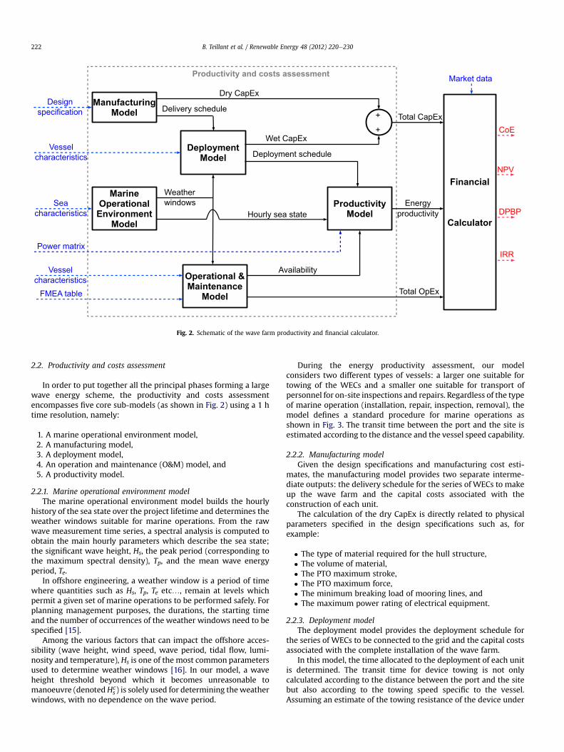
Fig. 2. Schematic of the wave farm productivity and financial calculator.

B. Teillant et al. / Renewable Energy 48 (2012) 220e230222

2.2. Productivity and costs assessment

In order to put together all the principal phases forming a largewave energy scheme, the productivity and costs assessmentencompasses five core sub-models (as shown in Fig. 2) using a 1 htime resolution, namely:

1. A marine operational environment model,2. A manufacturing model,3. A deployment model,4. An operation and maintenance (O&M) model, and5. A productivity model.

2.2.1. Marine operational environment modelThe marine operational environment model builds the hourly

history of the sea state over the project lifetime and determines theweather windows suitable for marine operations. From the rawwave measurement time series, a spectral analysis is computed toobtain the main hourly parameters which describe the sea state;the significant wave height, Hs, the peak period (corresponding tothe maximum spectral density), Tp, and the mean wave energyperiod, Te.

In offshore engineering, a weather window is a period of timewhere quantities such as Hs, Tp, Te etc., remain at levels whichpermit a given set of marine operations to be performed safely. Forplanning management purposes, the durations, the starting timeand the number of occurrences of the weather windows need to bespecified [15].

Among the various factors that can impact the offshore acces-sibility (wave height, wind speed, wave period, tidal flow, lumi-nosity and temperature), Hs is one of the most common parametersused to determine weather windows [16]. In our model, a waveheight threshold beyond which it becomes unreasonable tomanoeuvre (denotedHc

s ) is solely used for determining theweatherwindows, with no dependence on the wave period.

During the energy productivity assessment, our modelconsiders two different types of vessels: a larger one suitable fortowing of the WECs and a smaller one suitable for transport ofpersonnel for on-site inspections and repairs. Regardless of the typeof marine operation (installation, repair, inspection, removal), themodel defines a standard procedure for marine operations asshown in Fig. 3. The transit time between the port and the site isestimated according to the distance and the vessel speed capability.

2.2.2. Manufacturing modelGiven the design specifications and manufacturing cost esti-

mates, the manufacturing model provides two separate interme-diate outputs: the delivery schedule for the series of WECs to makeup the wave farm and the capital costs associated with theconstruction of each unit.

The calculation of the dry CapEx is directly related to physicalparameters specified in the design specifications such as, forexample:

� The type of material required for the hull structure,� The volume of material,� The PTO maximum stroke,� The PTO maximum force,� The minimum breaking load of mooring lines, and� The maximum power rating of electrical equipment.

2.2.3. Deployment modelThe deployment model provides the deployment schedule for

the series of WECs to be connected to the grid and the capital costsassociated with the complete installation of the wave farm.

In this model, the time allocated to the deployment of each unitis determined. The transit time for device towing is not onlycalculated according to the distance between the port and the sitebut also according to the towing speed specific to the vessel.Assuming an estimate of the towing resistance of the device under

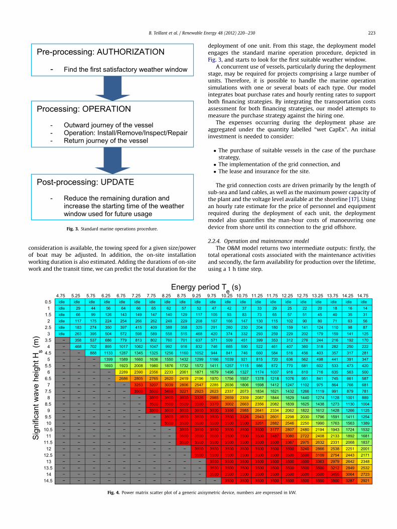
Pre-processing: AUTHORIZATION

- Find the first satisfactory weather window

Processing: OPERATION

- Outward journey of the vessel- Operation: Install/Remove/Inspect/Repair- Return journey of the vessel

Post-processing: UPDATE

- Reduce the remaining duration and increase the starting time of the weather window used for future usage

Fig. 3. Standard marine operations procedure.

B. Teillant et al. / Renewable Energy 48 (2012) 220e230 223

consideration is available, the towing speed for a given size/powerof boat may be adjusted. In addition, the on-site installationworking duration is also estimated. Adding the durations of on-sitework and the transit time, we can predict the total duration for the

4.75 5.25 5.75 6.25 6.75 7.25 7.75 8.25 8.75 9.25 0.5 1 1.5 2 2.5 3 3.5 4 4.5 5 5.5 6 6.5 7 7.5 8 8.5 9 9.5 1010.5 1111.5 1212.5 1313.5 1414.5

idleidleidleidleidleidleidleidleidleidleidleidleidleidleidleidleidleidleidleidleidleidleidleidleidleidleidleidleidle

idle 29 66 117 183 263 358 468 592 731 885105312361433164618722114237026402925322535003500350035003500350035003500

idle 44 99 175 274 395 537 702 88810961326157818532148246628063168350035003500350035003500350035003500350035003500

idle 56 126 224 350 504 686 895113313991693201523652742314835003500350035003500350035003500350035003500350035003500

idle 64 143 254 397 572 7791017128715891923228926863115350035003500350035003500350035003500350035003500350035003500

idle 66 149 266 415 598 8131062134516602008239028053253350035003500350035003500350035003500350035003500350035003500

idle 65 147 262 409 589 8021047132516361980235627653207350035003500350035003500350035003500350035003500350035003500

idle 62 140 248 388 558 760 992125615501876223326203039348835003500350035003500350035003500350035003500350035003500

idle 57 129 229 358 515 701 916116014321732206124192806322135003500350035003500350035003500350035003500350035003500

idle 52 117 208 325 468 637 832105212991572187121962547292333263500350035003500350035003500350035003500350035003500

−−−−−−−−−−−−−−−−−−−−−−−

−−−−−−−−−−−−−−−−−−−−−

−−−−−−−−−−−−−−−−−−−−

−−−−−−−−−−−−−−−−−−

−−−−−−−−−−−−−−−−

−−−−−−−−−−−−−−

−−−−−−−−−−−

−−−−−−−−−

−−−−−−

−−−−

Energy pe

Sign

ifica

nt w

ave

heig

ht H

s (m)

Fig. 4. Power matrix scatter plot of a generic axisy

deployment of one unit. From this stage, the deployment modelengages the standard marine operation procedure, depicted inFig. 3, and starts to look for the first suitable weather window.

A concurrent use of vessels, particularly during the deploymentstage, may be required for projects comprising a large number ofunits. Therefore, it is possible to handle the marine operationsimulations with one or several boats of each type. Our modelintegrates boat purchase rates and hourly renting rates to supportboth financing strategies. By integrating the transportation costsassessment for both financing strategies, our model attempts tomeasure the purchase strategy against the hiring one.

The expenses occurring during the deployment phase areaggregated under the quantity labelled “wet CapEx”. An initialinvestment is needed to consider:

� The purchase of suitable vessels in the case of the purchasestrategy,

� The implementation of the grid connection, and� The lease and insurance for the site.

The grid connection costs are driven primarily by the length ofsub-sea and land cables, as well as the maximum power capacity ofthe plant and the voltage level available at the shoreline [17]. Usingan hourly rate estimate for the price of personnel and equipmentrequired during the deployment of each unit, the deploymentmodel also quantifies the man-hour costs of manoeuvring onedevice from shore until its connection to the grid offshore.

2.2.4. Operation and maintenance modelThe O&M model returns two intermediate outputs: firstly, the

total operational costs associated with the maintenance activitiesand secondly, the farm availability for production over the lifetime,using a 1 h time step.

9.75 10.25 10.75 11.25 11.75 12.25 12.75 13.25 13.75 14.25 14.75idle 47 105 187 291 420 571 746 94411661411167919702285262329853370350035003500350035003500350035003500350035003500

idle 42 93 166 260 374 509 665 84110391257149617562036233726593002336635003500350035003500350035003500350035003500

idle 37 83 147 230 332 451 590 746 9211115132715571806207323592663298533263500350035003500350035003500350035003500

idle 33 73 130 204 293 399 522 660 815 986117413781598183420872356264129433261350035003500350035003500350035003500

idle 29 65 115 180 259 353 461 584 720 872103712181412162118442082233426012882317734873500350035003500350035003500

idle 25 57 102 159 229 312 407 516 636 770 91610761247143216291839206222982546280730803367350035003500350035003500

idle 22 51 90 141 202 276 360 456 562 681 810 9511102126614401625182220302250248027222975324035003500350035003500

idle 20 45 80 124 179 244 318 403 498 602 716 841 975111912741438161217961990219424082632286631093363350035003500

idle 18 40 71 110 159 216 282 357 441 533 635 745 864 99111281273142815911763194321332331253827542979321234553500

idle 16 35 63 98 141 192 250 317 391 473 563 661 766 87910011130126614111563172418922068225124432642284930643287

idle 14 31 56 87 125 170 222 281 347 420 500 587 681 781 8891004112512541389153216811837200121712348253227232921−

riod Te (s)

metric device, numbers are expressed in kW.

B. Teillant et al. / Renewable Energy 48 (2012) 220e230224

Currently, the O&Mmodel includes two scheduled maintenanceoperations, namely the on-site service and the mid-life refit.Assuming servicing a WEC on-site is possible for repair and/orinspection, the routine on-site visits are performed at a chosenfrequency (typically annual or bi-annual), the overhaul activityoccurs only once after the operational life of the device reaches halfof the WEC lifetime assumed. The mid-life refit involves the towingof each unit for onshore maintenance and therefore allows majorcomponent replacement.

Unscheduled maintenance is also simulated, based ona stochastic approach. Breakdown events are assumed to occurrandomly according to the likely frequency rates of failure given theFMEA table. Depending on the nature of the failure and the avail-ability of both the repair equipment and teams, the type of oper-ation and the recovery time is adjusted.

The expenses associated with every maintenance operation areassessed through the estimation of hourly rates, the cost of partsand the cost of vessel hire. In the end, the O&M model gives thehistory of the maintenance activities for each unit along with theimpact on both the availability for production and the O&M costs.

2.2.5. Productivity modelThe productivity model generates the hourly wave farm power

production over the lifetime, by combining the power matrix, theavailability and the wave measurements. For each hour, the energyproduction is given by the cell corresponding to the couple (Hs, Te)defining the sea state in the power matrix. In [18], a methodologyfor quantifying the effects of the farm lay-out on the productionand cost assessment is proposed. However, for the moment, ourmodel neglects constructive and destructive interferences thatoccur between devices in an array lay-out.

2.3. Financial calculator

Combining the outputs provided by the productivity and costassessment, the financial calculator gives an economic valuemeasure of a wave energy scheme. While the productivity and costassessment requires a 1 h time step, the financial calculator isexecuted on a yearly basis.

2.3.1. Market dataThe financial calculations of a project are subject to the estab-

lished financial and political policies governing the local marketwhere the project is undertaken. As an emerging industry, thewaveenergy sector is prone to evolving financial rules and policies. In theUK, the ROC is issued for eligible operators supplying electricity tothe national territory with green power for each MWh theyproduce. The nature and different aspects of the ROC are regularlybeing reviewed reflecting the evolving character of the renewableindustry [9].

In Ireland, a similar renewable energy feed-in-tariff (REFIT)programme is also currently under revision [19]. The financialcalculator can also be adapted to other price support mechanismse.g. renewable energy production tax credit, in the USA. For eachkWh of energy produced, the revenue obtained (denoted Rev in Eq.(1)) is given by the tariff secured by a REFIT-type program. At theend of each year, the total revenue generated is directly formulated.Since the period of time where the support price mechanismapplies may differ from the total duration of a project, the financialcalculator considers an average retail price of energy beyond thetariff duration of the price support mechanism until the end of lastyear of the project lifetime.

More traditional financial assumptions such as the tax rates areused in alignment with financial practice in related industries(offshore, renewable energy). For instance, the model has the

capability to simulate corporate taxes (including feed-in-tariffreductions) and the annual income tax deductions due to thedepreciation of the infrastructure.

2.3.2. Discounted cash-flow algorithmThe discounted cash-flow (DCF) technique tries to work out the

value of a project today, based on projections of how much moneyit is going to make in the future. Hence, the DCF analysis projectsthe amount of money that would circulate within the company orthe project with respect to the CapEx, the OpEx, the revenue anda discount rate.

Koller et al. [20] examine, with meticulous care, differentexisting approaches for the DCF method within various marketenvironmental conditions. To arrive at the yearly DCF, the standardprocedure is to calculate, firstly, the annual revenue and secondly,the annual taxes according to the financial environment (respec-tively denoted Rev(y) and Taxes(y) in Eq. (1)). Analytically, the DCFat each year y, as implemented in our model, is given by thefollowing expression:

DCFðyÞ ¼ FCFðyÞ�1þ Rd

100

�y

¼ RevðyÞ � OpExðyÞ � CapExðyÞ � TaxesðyÞ�1þ Rd

100

�y (1)

where Rd is the discount rate.

2.3.3. Financial indicatorsFor a given project lifetime, Y, our model uses the present value

(PV) approach to calculate the LCoE:

LCoE ¼ PVðCapExÞ þ PVðOpExÞPVðEPÞ (2)

where EP is the energy production in kWh and the PV of a cash-flow CF is defined as:

PVðCFÞ ¼XYy¼ y0

CFðyÞ�1þ Rd

100

�y (3)

and y0 is the first non-zero value year of the cash-flow CF.The NPV is obtained by adding all the discounted cash-flows

over the lifetime as demonstrated in Eq. (4). For a project to beprofitable, a strictly positive NPV at the end of the project isa necessary condition.

NPV ¼XYy¼0

FCFðyÞ�1þ Rd

100

�y ¼XYy¼0

DCFðyÞ (4)

In addition, the IRR is commonly used, along with the NPV, toassess the desirability of a project. The higher the IRR is above thediscount rate a project is expected to have, the more desirable it isto undertake the project. By definition, the IRR is the percentagewhich corresponds to the discount rate used in capital budgetingthat makes the NPV of all cash flows from a particular project equalto zero and can be conveniently defined as the solution of thefollowing equation.

XYy¼0

FCFðyÞ�1þ IRR

100

�y ¼ 0 (5)

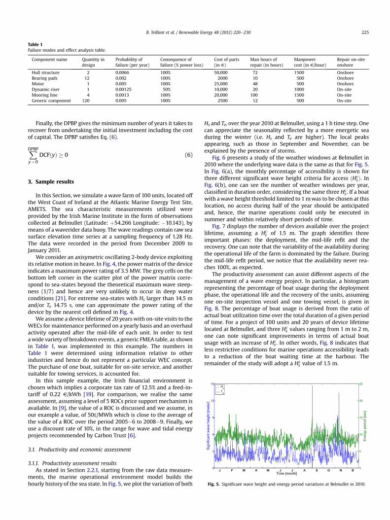
Table 1Failure modes and effect analysis table.

Component name Quantity indesign

Probability offailure (per year)

Consequence offailure (% power loss)

Cost of parts(in V)

Man hours ofrepair (in hours)

Manpowercost (in V/hour)

Repair on-siteonshore

Hull structure 2 0.0066 100% 50,000 72 1500 OnshoreBearing pads 12 0.002 100% 2000 10 500 OnshoreMotor 1 0.005 100% 25,000 48 500 OnshoreDynamic riser 1 0.00125 50% 10,000 20 1000 On-siteMooring line 4 0.0013 100% 20,000 100 1500 On-siteGeneric component 120 0.005 100% 2500 12 500 On-site

Fig. 5. Significant wave height and energy period variations at Belmullet in 2010.

B. Teillant et al. / Renewable Energy 48 (2012) 220e230 225

Finally, the DPBP gives the minimum number of years it takes torecover from undertaking the initial investment including the costof capital. The DPBP satisfies Eq. (6).

XDPBPy¼0

DCFðyÞ � 0 (6)

3. Sample results

In this Section, we simulate a wave farm of 100 units, located offthe West Coast of Ireland at the Atlantic Marine Energy Test Site,AMETS. The sea characteristic measurements utilized wereprovided by the Irish Marine Institute in the form of observationscollected at Belmullet (Latitude: þ54.266 Longitude: �10.143), bymeans of awaverider data buoy. Thewave readings contain raw seasurface elevation time series at a sampling frequency of 1.28 Hz.The data were recorded in the period from December 2009 toJanuary 2011.

We consider an axisymetric oscillating 2-body device exploitingits relative motion in heave. In Fig. 4, the powermatrix of the deviceindicates a maximum power rating of 3.5 MW. The grey cells on thebottom left corner in the scatter plot of the power matrix corre-spond to sea-states beyond the theoretical maximum wave steep-ness (1/7) and hence are very unlikely to occur in deep waterconditions [21]. For extreme sea-states with Hs larger than 14.5 mand/or Te 14.75 s, one can approximate the power rating of thedevice by the nearest cell defined in Fig. 4.

We assume a device lifetime of 20 years with on-site visits to theWECs for maintenance performed on a yearly basis and an overhaulactivity operated after the mid-life of each unit. In order to testawide variety of breakdown events, a generic FMEA table, as shownin Table 1, was implemented in this example. The numbers inTable 1 were determined using information relative to otherindustries and hence do not represent a particular WEC concept.The purchase of one boat, suitable for on-site service, and anothersuitable for towing services, is accounted for.

In this sample example, the Irish financial environment ischosen which implies a corporate tax rate of 12.5% and a feed-in-tariff of 0.22 V/kWh [19]. For comparison, we realise the sameassessment, assuming a level of 5 ROCs price support mechanism isavailable. In [9], the value of a ROC is discussed and we assume, inour example a value, of 50£/MWh which is close to the average ofthe value of a ROC over the period 2005e6 to 2008e9. Finally, weuse a discount rate of 10%, in the range for wave and tidal energyprojects recommended by Carbon Trust [6].

3.1. Productivity and economic assessment

3.1.1. Productivity assessment resultsAs stated in Section 2.2.1, starting from the raw data measure-

ments, the marine operational environment model builds thehourly history of the sea state. In Fig. 5, we plot the variation of both

Hs and Te, over the year 2010 at Belmullet, using a 1 h time step. Onecan appreciate the seasonality reflected by a more energetic seaduring the winter (i.e. Hs and Te are higher). The local peaksappearing, such as those in September and November, can beexplained by the presence of storms.

Fig. 6 presents a study of the weather windows at Belmullet in2010 where the underlying wave data is the same as that for Fig. 5.In Fig. 6(a), the monthly percentage of accessibility is shown forthree different significant wave height criteria for access ðHc

s Þ. InFig. 6(b), one can see the number of weather windows per year,classified in duration order, considering the same three Hc

s . If a boatwith awave height threshold limited to 1mwas to be chosen at thislocation, no access during half of the year should be anticipatedand, hence, the marine operations could only be executed insummer and within relatively short periods of time.

Fig. 7 displays the number of devices available over the projectlifetime, assuming a Hc

s of 1.5 m. The graph identifies threeimportant phases: the deployment, the mid-life refit and therecovery. One can note that the variability of the availability duringthe operational life of the farm is dominated by the failure. Duringthe mid-life refit period, we notice that the availability never rea-ches 100%, as expected.

The productivity assessment can assist different aspects of themanagement of a wave energy project. In particular, a histogramrepresenting the percentage of boat usage during the deploymentphase, the operational life and the recovery of the units, assumingone on-site inspection vessel and one towing vessel, is given inFig. 8. The percentage of boat usage is derived from the ratio ofactual boat utilization time over the total duration of a given periodof time. For a project of 100 units and 20 years of device lifetimelocated at Belmullet, and three Hc

s values ranging from 1 m to 2 m,one can note significant improvements in terms of actual boatusage with an increase of Hc

s . In other words, Fig. 8 indicates thatless restrictive conditions for marine operations accessibility leadsto a reduction of the boat waiting time at the harbour. Theremainder of the study will adopt a Hc

s value of 1.5 m.

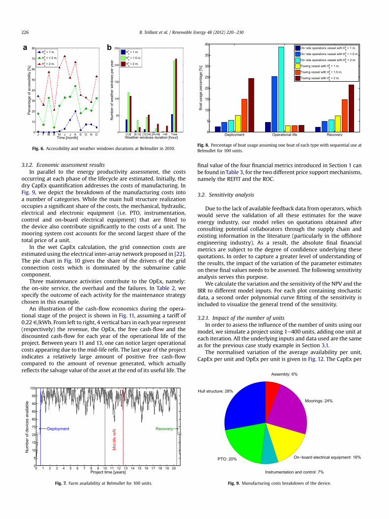
ba

Fig. 6. Accessibility and weather windows durations at Belmullet in 2010.Fig. 8. Percentage of boat usage assuming one boat of each type with sequential use atBelmullet for 100 units.

Assembly: 6%

B. Teillant et al. / Renewable Energy 48 (2012) 220e230226

3.1.2. Economic assessment resultsIn parallel to the energy productivity assessment, the costs

occurring at each phase of the lifecycle are estimated. Initially, thedry CapEx quantification addresses the costs of manufacturing. InFig. 9, we depict the breakdown of the manufacturing costs intoa number of categories. While the main hull structure realizationoccupies a significant share of the costs, the mechanical, hydraulic,electrical and electronic equipment (i.e. PTO, instrumentation,control and on-board electrical equipment) that are fitted tothe device also contribute significantly to the costs of a unit. Themooring system cost accounts for the second largest share of thetotal price of a unit.

In the wet CapEx calculation, the grid connection costs areestimated using the electrical inter-array network proposed in [22].The pie chart in Fig. 10 gives the share of the drivers of the gridconnection costs which is dominated by the submarine cablecomponent.

Three maintenance activities contribute to the OpEx, namely:the on-site service, the overhaul and the failures. In Table 2, wespecify the outcome of each activity for the maintenance strategychosen in this example.

An illustration of the cash-flow economics during the opera-tional stage of the project is shown in Fig. 11, assuming a tariff of0.22V/kWh. From left to right, 4 vertical bars in each year represent(respectively) the revenue, the OpEx, the free cash-flow and thediscounted cash-flow for each year of the operational life of theproject. Between years 11 and 13, one can notice larger operationalcosts appearing due to the mid-life refit. The last year of the projectindicates a relatively large amount of positive free cash-flowcompared to the amount of revenue generated, which actuallyreflects the salvage value of the asset at the end of its useful life. The

0 1 2 3 4 5 6 7 8 9 10 11 12 13 14 15 16 17 18 19 20 0

5

10

15

20

75

80

85

90

95

100

Mid

-life

refit

Project time [years]

Num

ber o

f dev

ices

ava

ilabl

e

Deployment Recovery

Fig. 7. Farm availability at Belmullet for 100 units.

final value of the four financial metrics introduced in Section 1 canbe found in Table 3, for the two different price supportmechanisms,namely the REFIT and the ROC.

3.2. Sensitivity analysis

Due to the lack of available feedback data from operators, whichwould serve the validation of all these estimates for the waveenergy industry, our model relies on quotations obtained afterconsulting potential collaborators through the supply chain andexisting information in the literature (particularly in the offshoreengineering industry). As a result, the absolute final financialmetrics are subject to the degree of confidence underlying thesequotations. In order to capture a greater level of understanding ofthe results, the impact of the variation of the parameter estimateson these final values needs to be assessed. The following sensitivityanalysis serves this purpose.

We calculate the variation and the sensitivity of the NPV and theIRR to different model inputs. For each plot containing stochasticdata, a second order polynomial curve fitting of the sensitivity isincluded to visualize the general trend of the sensitivity.

3.2.1. Impact of the number of unitsIn order to assess the influence of the number of units using our

model, we simulate a project using 1e400 units, adding one unit ateach iteration. All the underlying inputs and data used are the sameas for the previous case study example in Section 3.1.

The normalised variation of the average availability per unit,CapEx per unit and OpEx per unit is given in Fig. 12. The CapEx per

Hull structure: 28%

PTO: 20%

Instrumentation and control: 7%

On−board electrical equipment: 16%

Moorings: 24%

Fig. 9. Manufacturing costs breakdown of the device.

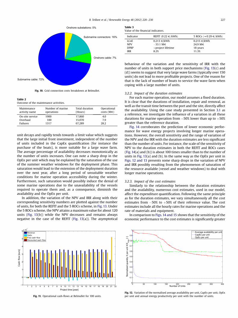
Table 2Outcome of the maintenance activities.

Maintenanceactivity name

Number of marineoperations

Total duration(Hours)

Operationalcosts (MV)

On-site service 1900 17,860 4.0Overhaul 100 15,070 7.9Failures 1317 67,289 28.2

Table 3Value of the financial indicators.

Indicator REFIT ð0:22 V=kWhÞ 5 ROCs ðz0:29 V=kWhÞLCoE 0.213 V/kWh 0.215 V/kWhNPV �33:1 MV 24.9 MV

DPBP >project lifetime 18 yearsIRR 8.2% 11.3%

Submarine cable: 72%

Onshore cable: 7%

Submarine connectors: 16%

Onshore substations: 5%

Fig. 10. Grid connection costs breakdown at Belmullet.

B. Teillant et al. / Renewable Energy 48 (2012) 220e230 227

unit decays and rapidly tends towards a limit value which suggeststhat the large initial front investment, independent of the numberof units included in the CapEx quantification (for instance thepurchase of the boats), is more suitable for a large wave farm.The average percentage of availability decreases monotonically asthe number of units increases. One can note a sharp drop in theOpEx per unit which may be explained by the saturation of the useof the summer weather windows for the deployment phase. Thissaturation would lead to the extension of the deployment durationover the next year, after a long period of unsuitable weatherconditions for marine operation accessibility during the winter.Furthermore, such saturation would possibly induce the denial ofsome marine operations due to the unavailability of the vesselsrequired to operate them and, as a consequence, diminish theavailability and the OpEx per unit.

In addition, the variation of the NPV and IRR along with theircorresponding sensitivity numbers are plotted against the numberof units, for both the REFIT and the 5 ROCs scheme, in Fig. 13. Underthe 5 ROCs scheme, the NPV attains amaximumvalue for about 120units (Fig. 13(b)) while the NPV decreases and remains alwaysnegative in the case of the REFIT (Fig. 13(a)). The asymptotical

Fig. 11. Operational cash-flows at Belmullet for 100 units.

behaviour of the variation and the sensitivity of IRR with thenumber of units in both support price mechanisms (Fig. 13(c) and(d)) seems to suggest that very large wave farms (typically over 150units) do not lead to more profitable projects. One of the reason forthat is the lack of number of boats to service the wave farm whencoping with a large number of units.

3.2.2. Impact of the duration estimatesFor each marine operation, our model assumes a fixed duration.

It is clear that the durations of installation, repair and removal, aswell as the transit time between the port and the site, directly affectthe availability. Using the case study presented in Section 3.1 asa reference, we investigate the influence of a variation in all thesedurations for marine operation from �50% lower than up to þ50%greater than the reference duration.

Fig. 14 corroborates the prediction of lower economic perfor-mance for wave energy projects involving longer marine opera-tions. However, the overall sensitivity and the range of variation ofthe NPV and the IRR with the duration estimates are less significantthan the number of units. For instance, the scale of the sensitivity ofNPV to the duration estimates in both the REFIT and ROCs cases(Fig. 14(a) and (b)) is about 100 times smaller than to the number ofunits in Fig. 13(a) and (b). In the same way as the OpEx per unit inFigs. 12 and 13 presents some sharp drops in the variation of NPVand IRR possibly resulting from the phenomenon of saturation ofthe resource available (vessel and weather windows) to deal withlonger marine operations.

3.2.3. Impact of the cost estimatesSimilarly to the relationship between the duration estimates

and the availability, numerous cost estimates, used in our model,affect the expenditure quantification. Following the same principleas for the duration estimates, we vary simultaneously all the costestimates from �50% to þ50% of their reference value. The costestimates include all the hourly rates for marine operations and therate of materials and equipment.

In comparison to Figs. 14 and 15 shows that the sensitivity of theeconomic performance to the cost estimates is significantly greater

Fig. 12. Variation of the normalised average availability per unit, CapEx per unit, OpExper unit and annual energy productivity per unit with the number of units.

a

c

b

d

Fig. 13. Variation and sensitivity of the NPV and the IRR with the number of units for the REFIT and 5 ROCs.

B. Teillant et al. / Renewable Energy 48 (2012) 220e230228

than to the duration estimates. In particular, one can note that ifa project developer achieves a reduction of 50% in all the cost esti-mates, the NPVwould be improved by about 100MVand the IRR byabout 7%. Subsequently, from a business perspective, it would bepreferable to allocate more resources in achieving reductions of thecost estimates over reductions of the duration estimates.

a

c

b

d

Fig. 14. Variation and sensitivity of the NPV and the IRR w

3.2.4. Impact of the tariffThe evolving character of the tariff, which each kW h produced

by a WEC attracts, motivates a further sensitivity study. As a result,Fig. 16 presents the variation and sensitivity of both the NPV andthe IRR with the tariff. The level of tariff offered by the REFIT andthe 5 ROCs are annotated with vertical lines.

ith the duration estimates for the REFIT and 5 ROCs.

a

c

b

d

Fig. 15. Variation and sensitivity of the NPV and the IRR with the cost estimates for the REFIT and 5 ROCs.

Fig. 16. Variation and sensitivity of the NPV and the IRR with the tariff.

B. Teillant et al. / Renewable Energy 48 (2012) 220e230 229

The tariff has as significant impact on the overall economicperformance as the costs estimates. For example, a tariff 50%greater than 0.22 V/kWh (the REFIT level of support assumed inthis paper) would potentially give an IRR of 13.2% compared to 8.2%for the reference case, which is significant, from an investorperspective.

4. Conclusion

In this paper, a tool for productivity and economic assessment ispresented and illustrated with a sample case study involving thedeployment of 100WEC units off theWest Coast of Ireland. The useof operational simulations for the assessment of the energyproductivity are tested for a variety of maintenance activities using

a standard methodology for every type of marine operationinvolved. The hourly quantification of the device availability andoperational costs is depicted and can offer guidelines for themanagement of a full scale wave energy plant. Four financialmetrics, including the NPV, IRR, LCoE and DPBP are also calculated,which demonstrate the capability of combining operational simu-lations and financial calculations to provide a wide range ofeconomic performance indicators, necessary to the evaluation ofthe profitability of a wave farm.

By performing a sensitivity analysis of different inputs of theassessment on the economic value, we show that it is possible toidentify the areas of aWEC technology that are of most influence onthe economic performance. As a result, a developer could optimisethe orientation of the allocation of development resources for

B. Teillant et al. / Renewable Energy 48 (2012) 220e230230

a particular WEC technology, based on an economic argument.Each of these, in turn, serves the purpose of achieving commercialwave energy application by accelerating the definition of anattractive and competitive project plan for prospective investors.

In time, as the wave energy industry matures, a dynamic usageof such a tool for economic performance assessment is indispens-able to adjust the quantification of the costs and the market envi-ronmental assumptions. Indeed, the model developed in this papermust be constantly updated as operational experience is gained inorder to refine and validate its estimates. Considering the low levelof maturity of the wave energy industry, it is difficult to obtainestimates for the design costs of a WEC technology and, therefore,the assessment presented here ignores them. The time and themanpower costs during the manufacturing phase are also ignoreddue to the almost complete lack of information relevant to therequirements for manufacturing a WEC. In the future, the designcosts as well as manpower manufacturing costs will need to beadded to the other costs featured in the assessment presented here.

In this paper, the power matrix has been used to evaluate thepower output of the WECs for varying sea conditions, based onspecification of the significant wave height, Hs and the wave energyperiod Te. However, we note that this type of power calculation canbe a little misleading for resonant WECs, since they are sensitive tothe particular sea power spectrum and various spectral shapes canhave identical Hs and Te values [23]. In particular, some seas mayhave little spectral power at the resonant frequency of theconverter. Nevertheless, the use of a power matrix providesa computationally simple method for power output evaluationcompared to a full time-domain simulation, with an error notexceeding that for the financial side calculations.

Acknowledgements

The financial support of Enterprise Ireland and Wavebob Ltd,under project IP/2009/0024 is gratefully acknowledged. In addition,the authors wish to express their acknowledgements to the IrishMarine Institute for providing real sea observations.

References

[1] Clement A, McCullen P, Falcao A, Fiorentino A, Gardner F, Hammarlund K, et al.Wave energy in Europe: current status and perspectives. Renewable andSustainable Energy Reviews 2002;6:405e31.

[2] Atkins Oil & Gas Engineering Ltd. A parametric costing model for wave energytechnology, tech. rep. ETSU report number wv-1685. The UK Department ofTrade and Industry and the Energy Technology Support Unit (ETSU); 1992.

[3] Thorpe TW. A review of wave energy, tech. rep. ETSU report number R-72. TheUK Department of Trade and Industry and the Energy Technology SupportUnit (ETSU); December 1992.

[4] Thorpe TW. A brief review of wave energy, tech. rep. ETSU report numberR-120. The UK Department of Trade and Industry and the Energy TechnologySupport Unit (ETSU); May 1999.

[5] Previsic M, Siddiqui O, Bedard R. Economic assessment methodology foroffshore wave power plant, tech. rep. EPRI; 2004.

[6] Callaghan J. Future marine energy, tech. rep. Carbon Trust; 2006.[7] Dalton G, Alcorn R, Lewis T. Case study feasibility analysis of the Pelamis wave

energy converter in Ireland, Portugal and North America. Renewable Energy2009;35:443e55.

[8] Raventos A, Sarmento A, Neumann F, Matos N. Projected deployment andcosts of wave energy in Europe. In. 3rd International conference on oceanenergy; 2010.

[9] Allan G, Gilmartin M, Mc Gregor P, Swales K. Levelised costs of wave and tidalenergy in the UK: cost competitiveness and the importance of bandedrenewables obligation certificates. Energy Policy 2011;39:23e39.

[10] Stallard T, Rothschild R, Aggidis G. A comparative approach to the economicmodelling of a large-scale wave power scheme. European Journal of Opera-tional Research 2007;185:884e98.

[11] Ricci P, Lopez J, Villate JL, Stallard T. Summary of attributes of cost modelsused by different stakeholders, tech. rep. D 7.1. EquiMar; February 2009.

[12] Menanteau P, Finon D, Lamy M. Prices versus quantities: choosing policies forpromoting the development of renewable energy. Energy Policy 2003;31:799e812.

[13] Weber J, Teillant B, Costello R, Ringwood J, Soulard T. Integrated WEC systemoptimisation e achieving balanced technology development and economicallifecycle performance. In. 9th European wave and tidal energy conference.Southampton, United Kingdom; 2011.

[14] Stallard T, Johanning L, Smith G, Ricci P, Villate JL, Dhedin JF. Guidelinesregarding the variation of infrastructure requirements with scale of deploy-ment, tech. rep. D 7.3.3. Equimar; February 2010.

[15] Graham C. The parameterisation and prediction of wave height and windspeed persistence statistics for oil industry operational planning purposes.Coastal Engineering 1982;6:303e29.

[16] Det Norske Veritas. Modelling and analysis of marine operations, tech. rep.DNV-RP-H103. Det Norske Veritas; 2011.

[17] O’Sullivan D, Dalton G. Challenges in the grid connection of wave energydevices. In. 8th European wave and tidal energy conference. Uppsala, Sweden;2009.

[18] Beels C, Troch P, Kofoed J, Frigaard P, Kringelum J, Kromann P, et al.A methodology for production and cost assessment of a farm of wave energyconverters. Renewable Energy 2011;36:3402e16.

[19] The Department of Communication. Energy and natural resources of theRepublic of Ireland, renewable energy feed-in-tariff, Minister Ryan launchesmajor new ocean energy initiatives; 2009.

[20] Koller T, Goedhart M, Wessels D. Measuring and managing the value ofcompanies. John Willey & Sons, Inc.; 2005.

[21] U.S. Army Corps of Engineers. Coastal engineering manual (CEM) e part 2:coastal hydrodynamics e chapter II-1: water wave mechanics, tech. rep. EM1110-2-1100. U.S. Army Corps of Engineers; 2002.

[22] Sharkey F, Bannon E, Colon M, Gaughan K. Dynamic electrical rating and theeconomics of capacity factor for wave energy converters arrays. In. 9thEuropean wave and tidal energy conference, Southampton, United Kingdom;2011.

[23] Nolan N, Ringwood J, Holmes B. Short term wave energy variability off thewest coast of Ireland. In. 7th European wave and tidal energy conference.Porto, Portugal; 2007.