Products of Polynomials in Many Variables

IOURNAL OF NUMBER THEORY 36, 219-245 (1990)

Products of Polynomials in Many Variables

BERNARD BEAUZAMY

Ins&w de Calcul MathPmatique, UniversitP de Paris 7. Paris, France*

ENRICO BOMBIERI

Institute for Advanced Study, Princeton, New Jersey 08540’

PER ENFLO

Kent State University, Kent, Ohio 44242’

HUGH L. MONTGOMERY

University of Michigan, Ann Arbor, Michigan 48109’

Communicated by H. Zassenhaus

Received July 12, 1989

We study the product of two polynomials in many variables, in several norms, and show that under suitable assumptions this product can be bounded from below independently of the number of variables. 0 1990 Academx Press. Inc.

INTRODUCTION

In this paper, we let

P(x,, . ..) XN) = c a,x;‘. . . xol,“, Q(x,, . ..) XN) = c bpxf’ . . . x9, a B

* Supported in part by Contract 89/1377, Ministry of Defense, DGA/DRET, France. ’ Supported in part by a grant from the National Science Foundation, U.S.A.

219 0022-314X/90 $3.00

Copyright #; 19W by Academic Press, lnc All rights of reproduction in any form reserved.

220 BEAUZAMY ET AL.

with ~1= (a,, . . . . a,), /I= (PI, . . . . BN), be polynomials in N variables, Xl, *.-, XN, and with complex coefficients. We are interested in estimates from below for the product PQ, that is in estimates of the form

IlPQll 5 ,J IIPII . 111211 2

for some norm )I . )) on the space of polynomials.

The norms we use are first related to the coefficients of P,

IPlp=(C lbAP)“‘, Ix

for 1 <‘p< cc, and

(1)

JP(, =max (u,I. a

Other norms, also related to the coefficients of P, are

IPlp=(C(~)” k4yp, bl

where m is the total degree of P, and cr! = a, ! . . . tlN ! . Comparison between these norms is given by the following inequalities:

1 ( )

1 - UP

z IPI, d CPI, G IPIp. (2)

We can also consider P as a function on the polycircle, and introduce the Lp norms

J(P(I, = ( jIz . . . J-; Ip(eiy . ..) e’fyIP 2.. .tg!$

for 1 <p<cc, and

JJPI( m = max JP(eiel, . . . . eiBN)J . 81 I . . . . ON

We observe the following relations between the norms already intro- duced:

IPls,~ll~ll,~ll~l12=l~12~ll~ll~~I~I~~

Of course, for 1 G p si q < co,

lIPlIp G IIPIIq.

PRODUCTSOFPOLYNOMIALS 221

Moreover, as we see in Section 1, there is a constant Cm,p.y > 0 such that if P is a polynomial with (total) degree at most m,

IlPII,B cm,p,q IlPIl,. For the I.\,,-norms, we have, for l<p<q<a;,

but there is no constant depending only on the degree (and independent of the number of variables) such that the converse inequality holds: this is clear from the consideration of the example P = (xl + . .. + xN)/N.

In the case of polynomials in one variable, estimates of the type (1) were obtained, under specific assumptions, by B. Beauzamy and P. Enflo [l]. They of course extend to polynomials in several variables, but lead to estimates which depend on the number of variables.

We are interested here in estimates independent of the number of variables. The first result of this nature was obtained by P. Enflo [2], in the frame of concentration at low degrees. To define it, let (c(/ = IX, + . . . + LX,,,. Then we say that P has concentration d (0 < d Q 1) at degree k if

c I4 2 dC la,l.

Then the theorem in [2] is:

THEOREM. There is a constant A(d, d’; k, k’) > 0 such that for any polynomials P and Q, with concentration d at degree k, concentration d’ at degree k’, respectively, one has

IPQIIZ~. lPl,.lQl,.

The important point is that the constant 1 does not depend on the degrees of the polynomials, nor on the number of variables.

We study here similar problems, in various norms, as was done in [ 11; moreover the proof given here in the case of the 1. / i-norm is simpler than the original proof of [a]. For all these reasons, the present paper may be regarded as a continuation of [ 1,2].

It is convenient for us to start with homogeneous polynomials.

1. HOMOGENEOUS POLYNOMIALS

In this section, P and Q are homogeneous polynomials of degrees m and n, respectively:

p(X~,-.,X,v)= c a,x;‘...x”,N, Q(x ,,..., x,)= C hsxfl...XS,N. (1) 1x1 =m IPI =n

222 BEAUZAMYETAL.

Then we have:

THEOREM 1.1. There exists a constant C,(m, n) > 0 such that, for any polynomials P and Q, homogeneous of degrees m and n, respectively, one has, for anyp, lQpdco,

C,(m,n)lPI,~lQ[,~~PQ~,~2~m+")"-"~)lPlp~lQl,.

No information is given about the value of C,(m, n) in general. But in the case p = 2, precise bounds are obtained for the norm [ .]* :

THEOREM 1.2. Let P, Q be homogeneous polynomials of degrees m, n, respectively. Then

and this estimate is best possible.

For the )I . lip-norms, we obtain:

THEOREM 1.3. There exist constants C2(p, m, n) > 0 and C;(p, m, n) > 0 such that, for any polynomials P and Q, homogeneous of degrees m and n, respectively, one has, for any p, 16 p < co,

CAP, m, n) llPllP~ IlQll, < IlPQll,~ C;(P, m, n) Ilf’ll, . IIQllp,

and in the case p = 03,

with

G(a, m, n) IPII, IIQII, i IIPQII, 6 IPII, IlQlL,

inf(m, n)

CJcqm,n)= l-j tan* (2k- 1)~

k=l 4(m+n) ’

In order to prove Theorem 1.1, we start with some basic inequalities for the I, norms. The first one gives the upper estimate in Theorem 1.1.

A. Relations between Norms

LEMMA 1.A.l. For 1 <pi co,

lPQlp<22(m+n)(1-1’p) (P(;JQJ,.

Proof of Lemma 1.A.l. We write

PQ = c c,,x;’ . . . xyNN.

PRODUCTSOF POLYNOMIALS

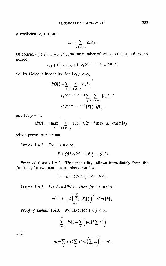
A coeffkient cl, is a sum

223

c,= 2 a,bp. x+p=;

Of course, a, < y 1, . . . . tlN < y,,,, so the number of terms in this sum does not exceed

So, by HGlder’s inequality, for 1 < p < 00,

iPei:=Zl c u,bpi’ y a+/?=s

<2(m+n’(pp1)x 1 la,bglP .; z+p=y

<2’m+n)(p-1) Ipl”p IQ\;,

and forp=co,

l~Ql,=m~~~~~sa,bp~h2m+“maxia,l~m~xIh,l,

which proves our lemma.

LEMMA l.A.2. For 1 <p< co,

l~+Ql~~~P-l~l~l~+lQI~~~

Proof of Lemma l.A.2. This inequality follows immediately from the fact that, for two complex numbers a and b,

(a+blP~2P-1()a1p+lblP).

LEMMA l.A.3. Let P,=aP/ax,. Then, for 1 <p< 00,

Proof of Lemma l.A.3. We have, for 1 < p < 00,

and

I 1 L >

P

m=Cai<CaP< Cai =mp,

224 BEAUZAMYETAL.

from which the lemma follows. Modifications in the case p = co are obvious.

We now turn to the proof of Theorem 1.1. Let k, m, n E N, and let C,(m, n) = C,(p, m, n) be the largest real number such that the inequality

holds for all homogeneous polynomials P, Q of degrees m, n, respectively. Clearly, 0 < C,Jm, n) < 1. Our object is to show that Ck(m, n) > 0 for

every k, m, II E N: taking k = 1, we get the theorem. This is accomplished by an inductive argument, the basic steps of which are fulfilled in the following two lemmas:

LEMMA l.A.4. For 1 <p < co,

Ck+ ,(m, 0) 2 ml’P-lC,(m - 1, mk) . C,(m, 0).

Proof of Lemma l.A.4. We assume p < co, the case p = 0~) being left to the reader. For any homogeneous polynomial P of degree m, with the notation of Lemma l.A.3, we have, for every i,

I(Pk+l)&= (k+ 1) lPiPklp

Z (k+ 1) C,(m - 1, mk) lpilp IPklp

2 (k + 1) C,(m - 1, mk) Cdm, 0) If’ilp IPIp”

which implies

By Lemma l.A.3,

which gives the desired result.

LEMMA l.A.5. For 1 <p < co,

Ck(my n) 2 Ck + 1 (m,n-1)n’/P[(km+n)P+(km)P]-1/~2-(1--/P)(km+m+n).

Proof of Lemma l.A.5. Again, we treat only the case p < 00. We have, for every i,

PRODUCTS OF POLYNOMIALS 225

Ck+,(m,n-l)PIPI~+l)PIQil~,IP’+‘Qil~

= IP(PkQi+kPk-‘Pie)-kPkPiQl;

<2P-1((P(PkQi+kPk-1PiQ)l;

+kP lPkPiQl z)v by Lemma l.A.2

<2(J’-1’(km+m+n)(lpl; IpkQ,+kpk-‘p,Q(;

+ kP lPkQl; IPi1 ;,> by Lemma 1.A.l.

But PkQi+kPk--‘PiQ=(PkQ),.. W e sum both sides over i and apply Lemma l.A.3. We find

nCk+l @~,n-l)~IPj~+~)~lQl;

~2(P~1)(km+m+n)((km+n)P IPI; lPkQIP,+kPmp IPj”p IP”Ql”,),

which implies

)PkQ(p~Ck+l(m,n-l)n”P[(km+n)P+(km)P]~l’P

X2-11-l/~)(km+m+n) IPI; lQlp,

and shows the result.

We now complete the proof of Theorem 1.1. By induction on m, we show that, for every n > 0,

C,(m, n) > 0. (1)

Clearly, Cr(0, n) = 1. Assume we know that

C,(m - 1, n) > 0, for all n > 0. (2)

First, we show that, for every k > 1,

Ck(m, 0) > 0, for all m > 0. (3)

This is done by an induction on k: C,(m, 0) = 1, and the inductive step on k is made by Lemma l.A.4, using (2). So (3) is proved.

Next, we show that

Ckh n, > 0, for all k, m, n > 0. (4)

This will be done by an induction on n. For n = 0, this is (3). Assume that C,(m, n - 1) > 0 for all k, m. Using Lemma l.A.5, we find that C,(m, n) > 0 for all k, m. This proves (4), which implies (1).

The constants occurring in all lemmas are uniformly bounded in p, 1 d p Q co, so in the final result we may give a constant independent of p.

226 BEAUZAMYETAL.

Remark 1. Similar results can be obtained in the case 0 < p < 1 (where ( .IP is only a quasi-norm); the constants then depend on p and become worse and worse when p + 0.

Remark 2. If we consider the case p = 1, m = n = k = 1, Lemma l.A.4 gives C,(l, 0)= 1, and Lemma l.A.5 gives Ci(1, l)>$. Thus

for homogeneous polynomials P, Q of degree 1. But (at least for real coefficients), a better estimate can be found:

LEMMA l.A.6. Let P, Q be homogeneous polynomials of degree 1, with real coefficients. Then

lPQl~~#'l, IQI,,

and this estimate is best possible.

ProoJ We write P= CT aixi, Q = CF bixi, with C Iail = C /bi( = 1. We can assume that all the hi’s are >O, and that for some n (1 <n -C N), a, > 0 if i < n, and ai 6 0 if i > n. We set tl= CT ai, p = C; bi, and

&c, y)=ax-(1 -a)y,

&<X> y)=Px+(l-P)Y.

Then one checks easily that

lPQl&I~~l,~~~

and this value is attained when IX= I= 1.

The above remark and this result show that the method of proof of Theorem 1.1 does not produce constants which are best possible.

We now turn to, the proof of Theorem 1.2.

B. The Norms Deduced from Taylor’s Formula

We have defined the [ .I,-norms in the Introduction. In the case of homogeneous polynomials, they are related to Taylor’s formula as follows.

For a polynomial P(x,, . . . . x,), homogeneous of degree m, we can write

N

ml 9 -.*, x,,=' c av

m! i, __, im= 1 ax,, . * . axim xi, "'Xi,.

9 . If P is written as before,

P(x 1, ‘.., x,)= C a,x;l . ..x*N”. Ial =m

PRODUCTS OF POLYNOMIALS

the norm [PI, defined as

227

[P],=( c ($)p-l ,aqp, lal=m . with a! = CI~ ! . . . c(~ ! , satisfies clearly

We define k,(m, n) as the largest constant A B 0 such that the inequality

l321, B 431, CPI,

holds for all IV, all polynomials P, Q in N variables, homogeneous of degrees m, n, respectively.

Theorem 1.2 asserts that k,(m, n) = Jm! n!/(m + n)!. It is derived from a statement about functions, which we now describe.

Let 24= (u,, . . . . u,), u= (u,, . . . . II,), and let F(u), G(u) be functions on the unit cubes I”, I”, with complex values, and invariant under the symmetric groups YM, Z$, respectively. Let also w = ( wl, . . . . w, + .), and define a shzq’jk of type (m, n) to be

(4, f) = (4, . . . . i,; j,, . . . . j,),

where i,<i,< ... <im,jl<jZ< . . . <jn, and (,a,%) is a permutation of the set {1,2, . . . . m+n}.

The set of shuttles of type (m, n) is denoted by sh(m, n), and its cardinality is

We write x,/ for (xi,, . . . . xi,). We now define cp(m, n) as the largest constant p 2 0 for which the

inequality

II c f;(xs) G(Q) 2 P IIFll.p(,m) IIGIILp(~n)

c.l.,f,~sh(m,n) II qm+n)

holds for all symmetric functions FE &(I”), G E L,(I”). The two constants k,(m, n) and c,(m, n) are related by:

LEMMA 1.B.l. Forallp, l<p<oo,allm,n~N,

m! n! k,(m, n) = (m + n)! cph n).

64136:2-l

228 BEAUZAMY ET AL.

Proof of Lemma l.B.1. (a) We first show that

m! n! kp(m9 n) 2 (m + n)! c,(m, n).

Let F, G be continuous symmetric functions on I”, I”, respectively. We define (with variables in P as capital letters)

(2) ml 3 *--, X,) = N -@P . ..x.,

QWl, . . . . X,)=N-“‘P F (3) im+l,...,im+.=l

These polynomials are of degree m, n, respectively, with N variables. So

and

[PI,= N- (

This last quantity tends to )I PII Lpc,mj when N + co, by approximation of the integral by means of Riemann sums.

We also have

pQ=N-(m+n)/F $

il,...,im+.= 1

F($ ,..., $G(% ,..., +“)Xi ,... X,+“,

[pQl,=:-L+;‘;( 5 1 c m . jl,....jmtn= 1 ii1 . . . . . im+#}= {jI ,.... jmcn} F($...,$)

L+l (‘ bl+ll P UP

XG -, . ..) - N )I) N

m! n! +(m II

c F(x~) G(x/) 9 (I,j)csh(m,n) II Lpp+n)

and this proves our first claim, first for continuous functions, then for all functions in Lp, p < cc, and finally for p = co.


(b) We now show the converse inequality. If P, Q are homogeneous polynomials as before, we define

F(.r 1, ...g x,)=1 i7”P

m! ax,, . . . ax,“,

where i, = [Ns,] + 1, . . . . i,,= [Nx,,,] + I. So F is constant in each cube, and therefore

G being defined the same way from Q, we get

IlGll &(P)= N --“TQlp

and

Fb,) W,) (f,,f)esh(m.n) ;I I +(lm+“)

amp anQ (3, f ) E shim. n)

ax,,...ax, ax,, --ax,

EN-('"+")'P(m+n)! yplln) V'QL I .

and the lemma is proved. It will allow us to compute precisely k,(m, n). First we show:

THEOREM l.B.2. For all F, G which are yt’,, Y* invariant,

Proof. We have

230

But

BEAUZAMYETAL.

5 F(x,) c(x,.) F(x,.) G(x,) dx, dx,

2

= 0 yn.mW(z,Xbn/Wz dx,,,,dx,,+O,

and this proves Theorem l.B.2. Theorem 1.2 now follows from Theorem l.B.2 and Lemma 1.B.l.

The estimate (m + n)!/m! n! in Theorem l.B.2 (and therefore the estimate of Theorem 1.2) is best possible. Indeed, take

F(x x,) = 1, G(x 1, . ..) X”) = e Zin(.q + ‘, + x.) 1, .‘.,

Ii Ii

2

c F(x,) G(x,) (m+n)!

= -

(~,f)~sh(m.n) L2(lm+n) m! n! ’

Remark. From Theorem 1.1 and the comparison estimates

1- IlP

IPIp < CPI,~ If?p, (4)

it follows that k,(m, n) > 0 for all p, 1 <p < co, and therefore that c,(m, n) >O. But for p # 2, we do not know the precise value of these constants.

These theorems have some consequences: First, we observe that Lemma l.A.6 and Lemma l.B.1 show that iff; g

are real-valued functions,

Jb’ f’ If(x) g(y) +f(y) g(x)1 dx 42 j’ I.0 )I d (0 x x>(o

j’ lg(y)l dy

We also deduce from (4):

PROPOSITION l.B.3. If P, Q are homogeneous polynomials of degrees m, n,

lPQ12ad& IPI,. 1912.


As we already said, this estimate is independent of the number of variables, and we do not know how precise it is. However, in the case of two variables, it can be greatly improved:

PROPOSITION l.B.4. Let P, Q be homogeneous polynomials of degrees m, n, with two variables. Then

lf’Ql,a(mm+n)-1’2 ( Em;z,)-1’2 ( I,:z,)l’z lplz 11212.

Proof of Proposition l.B.4. From Theorem l.B.1, we get

[PQ12~(mm+n)-1’2 CPl2 [Ql,.

But [ .I2 < 1. J2. Moreover, in the case of two variables, we have:

LEMMA l.B.5. Let P be a homogeneous polynomial of degree m, with two variables. Then

[PI2 2 [my2l - “2 PI,. ( >

Proof of Lemma l.B.5. One uses the fact that, if a1 + u2 = m,

aI. 1 a,! > [m/2]! (m - [m/2])!,

Proposition LB.3 follows immediately from the lemma.

Remark. A previously known bound, in the case of two-variable polynomials, was

lPQ12~(‘m”)~1’z(2,n)~1’2 IPI IQ12

& IPI2 lQl2. 2

Indeed, set f(z) = P(z, 1). The above formula is easily deduced from the comparison between Mahler’s measure,

M(f) = exp jin log If (@)I 2,

and the L,-norm off, Ilf IILz= (PI 2: see Mahler [4]. The bound given in Proposition l.B.4 is slightly better.

We now turn to the estimates related to the L,-norms.

232 BEAUZAMYETAL.

C. Estimates in L,-Norms

We now prove Theorem 1.3, first in the case p < 00. Since llPllz = IPlz, the result is known in the case p = 2. It follows for other values of p by comparison arguments between the various norms. The constants involved, of course, have to be independent of the number of variables.

LEMMA 1.C.l. Let P be a homogeneous polynomial of degree m. Then

I/P112< llPllpd2([‘082P’+‘)ffl’2 /[PI/*, if 2<p<co,

2-” lIPlIz d llPll,G IlPll2~ if lGpd2.

Proof of Lemma 1.C.l. By Parseval’s identity,

llpll:= IIp’II;= PI:.

By Lemma l.A.1, with P = Q,

IP21:<22m IPI&

and thus

IIPII‘I G F2 lIPlIz. (1)

Let now 12 1. We have

IIPII *,+, = IIpqy

Q (2 2’-‘m/2 I(pP’~~*)l/P’, by (1)

<2”/2 llp2’-‘/1;/2’-’

= 24 I/ PIJ 21,

and therefore, for 12 1,

Now, for p > 2, one chooses I = [log, p] + 1 and obtains the estimate. We now consider the case p < 2. The inequality )I PIJ, < 1) PII 2 is obvious.

The other inequality needs to be proved only in the case p = 1. But then we have

IIPII, G IIPII :Y3 . lW3

< 2”‘3 11 PJI :‘3 . 1) PJI :‘3, by (1).

so

llPl11>2-m IIPll*,


and our lemma is proved. Theorem 1.3, in the case p < co, follows immediately.

We now consider the case p = co. Then Lemma l.c.1 is not true anymore, as the example of P = x1 + . . . + xN shows. The right hand side inequality is obvious. We now prove the other one.

Let t = (tl, . . . . tNh r = (rl,, . . . . qN) be points on the polycircle Ixi( = 1 such that

IP(t)I = max IP(x,, . . . . x,~)I, 1;,1 = 1

IQ(s)1 = ,y”=“1 lQ(x,, . ..I .x,v)/. r,

We now consider, for 0 < t < 1,

.f(t)=P(tt+(1-t)rl), g(t) = Q(t5 + (I- 1) ~1.

Since max,,, = 1 (P(x,, . . . . xN) Q(x,, . . . . xN)l is attained on the Shilov boundary lxil = 1, we see that

IIPQII m 2 oy:, If(t) s(t)l. . .

Our result now follows immediately from the following theorem of Kneser c31:

THEOREM (H. Kneser). Letf(z), g(z) be polynomials of degrees m, n and let E be a bounded continuum in @. Then

my If(z) &)I 3 @, n) yx If( my I&)l 3

where

c(m, n) = fi tan’ (2k- 1)rc

k=l 4(m+n) ’

Equality is attained if, setting z = cos 4, f(z) g(z) = cos(m + n) 4, and

f(z)= fi (z-cos($-;;;). k=l

To finish this section, we observe the estimate

inf(m, n)

C,(co,m,n)= n tan’ (2k-l)rr 1

k=l 4(m+n) ‘4”‘”

We now turn to polynomials which are not necessarily homogeneous.

234 BEAUZAMYETAL.

2. POLYNOMIALS WITH CONCENTRATION AT Low DEGREES

Let, as before,

w, f . . . . XN)=Cuaxc;‘-.x$+ 01

be a polynomial in many variables. We set a = (u.,, . . . . a,,,), (a( = a1 + ... -t~1~, and, for kE N, we put

PI% c a,xc;‘...xF. la1 Gk

Let 0 < d< 1. We say that P has concentration d at (total) degree k, in a norm 11 . (1, if

IIPlkll 2 d IIPII .

This applies for instance to any of the norms I -IP, )I 1 lip defined in the previous paragraph.

We extend to this new frame the results previously obtained for homogeneous polynomials. First, we extend them to polynomials of fixed degrees, with bounds dependent on the degree.

THEOREM 2.1. For any p, 1 < p < CO, any polynomials P, Q of degrees m, n, respectively,

C,(m, n) IPIp lQl,< IPQlp<2(m+n)c1-1’p) IPI, lQlp,

where C,(m, n) is the constant defined in Theorem 1.1.

THEOREM 2.2. For any p, 1 < p < oc), any polynomials P, Q of degrees m, n, respectively,

CAP, my n) lIPlIp IIQII, G IIf’Qll, < C;(P, m n) llpll, IIQllp,

and in the case p = co,

G(~, m, n) llpll, IIQII, G IIPQII, G llpll, IIQII,~

where C,(p, m, n), C;(p, m, n) are the constants defined in Theorem 1.2.

These theorems are immediately deduced from Theorems 1.1 and 1.2. Indeed, if P(x,, . . . . xN) is any polynomial of degree m, we put

P*(xo, X1) . ..) x,) = x;;P (2, . . . . Z)>

PRODUCTSOF POLYNOMIALS 235

and P* is homogeneous of degree m. Moreover, (PQ)* = P*Q*, (PI,= lP*lp, ((P(J,= l(P*jI,. The theorems follow.

We now turn to polynomials with concentration at low degrees. Let

Q(x,, . . . . xN)=c l+xf'--xF P

satisfy

IWlp34Plp (1)

lQl"lpad' IQlp. (2)

THEOREM 2.3, Let 1~ p < co. For m, n E N, 0 -C d, d’ < 1, there is a constant A(p; d, d’; m, n) > 0 such that, for any polynomials P, Q satisfying (11, (2)1

IU’QY+“l,z~ IPI, IQI,.

Proof of Theorem2.3. We may assume IPIp= lQlp= 1. For ic N, we write Pi for the homogeneous part of P of degree i, that is,

Pi= C aSxT1...xaNy. (a( = I

We give the proof for p < 00 and leave it to the reader for p = 00. Condition (1) implies

Therefore, for some il < m,

lpi,Ip 2 (m ,“1 )rip’

The same way, for some j, <n,

IQjllp 2 (n +d;)llp-

By Theorem 1.1, with A, = A,(p; m, n; d, d’),

IPi,Q,,Ip~L

(3)

(4)

(5)

236 BEAUZAMY ET AL.

Set R = PQ. Then

Ril+ji= C PiQj, (6) i+j=il+jl

In this sum, either i < i, or j < j,, and il + j, <m + n. So the sum has at most (m + n)2 terms. We have two cases:

- Case 0:

IRil+j,lp>$Alv

and the conclusion is reached, or

- Case 1:

In this case, by (6),

c (i,j)#(il,jl),i+i=ii +A

IPiQ~l~~~J~,.

So we can find iz, j2, with either i, < il or j, < jl, such that

IPi2Qjzlp 2 A23 (7)

with 3 d,=iLL

2 (m+n)*’

By Lemma l.A.3, since i2 < m + n, j, < m + n,

lPi2Qjzlp G C(P, m, 4 IPizIp lQj*lp, (8)

with C(p, m, n) = 22(” +n)(l - I’*), and, with 1; = 1,/C(p, m, n),

lpi*Ip 2 ni9 IQjzlp 2 A;* (9)

Assume first i, < i,. We look at the product Pi,Qj, 3 and we have, by Theorem 1.1,

IPizQjllp 2 A33

and we have two cases:

- Case 1.0:


and

- Case 1.1:

If i, > i,, then j, < j,, and we do the same with P,, Q,, instead.

We repeat this process. If we fall into a Case 0, the conclusion is reached. Otherwise, we find indexes ik, j,, such that for every k either ik < i, _, or j, < j, _ 1. Therefore, the number of steps is at most m + n: then we reach polynomials of degree 0, for which the conclusion is clear.

We now look at the L, norm. There is a substantial difference from the 1, norm, which has to be mentioned first. Obviously, one has

IPly? 6 IPI,.

A similar estimate,

with an absolute constant C, cannot hold in the L, norm. Indeed, the exponential system is not a l-unconditional basis in L,, so there is a polynomial fin one variable such that

and one considers P(x,, . . ..x.)=f(xl)...f(xN). On the other hand, we have:

LEMMA 2.4. For every p, 1 < p < 00, every polynomial P with N variables,

IlfYllpf(2m+1+1) lIPlIp.

Proof of Lemma 2.4. We assume 11 PII, = 1. We first consider the case p >, 2. By the Marcinkiewicz interpolation theorem, to prove our formula for p < co it is enough to prove it for p = 2,4, . . . . Then, letting p + CO, we also get it for p = 00.

So we take p = 2k, k 2 1. We have the obvious formula:

lIpIl,, = Ilpkll:‘*. (10)

Let, as before, P, be the homogeneous part of P of degree m. Let

R,=P,+P,+,+ ...

238 BEAUZAMYETAL.

In RL, the only terms of degree km are P”,. Since the L, norm is unconditional, we get

and by (10)

IIPi,ll :‘k G ll%ll :‘k,

IIPmII, 6 IlRnllp.

Since R,, , = R, - P,,,; we deduce

llR,+ lllp d 2 IIRnllp,

and inductively

II&II, G 2” IlRollp = 2”.

Since PI m = P - R, + , , we obtain

IIPlrnll,~ 1 +2”+‘,

which is our claim. So the lemma is proved for p > 2. The case 1~ p < 2 follows if we consider the operator P + PI m, from L, into itself: its trans- pose is the same operator, from L, into itself (l/p + l/q = 1).

We may now state our result for the L, norms:

THEOREM 2.5. Let 1~ p < 00. For m, n E N, 0 < d, d’ < 1, there is a constant A’(p; d, d’; m, n) > 0 such that, for any polynomials P, Q satisfying

IIPlmll,~ d lIPlIp,

IIQl”llp 2 d’ IIQllp,

one has

IIV’QI m+nllp 2 1’ IIPII, llQll,~

The proof is identical to the one of Theorem 2.3, except that, in order to get (9) in this proof, one uses Lemma 2.4.

We now turn to the following question: when does the product PQ have a large coeffkient?

3. LARGE COEFFICIENTS

Let again P and Q be polynomials in many variables. Assume that P has a large coefficient and that Q has a large coeffkient at low degrees. Then


we prove that the product PQ has a large coefficient, with estimates independent of the number of the variables. We obtain precisely:

THEOREM 3.1. Let 0 < d, d’ d 1, and k E N. There is a number A(d, d’; k) such that for any polynomials P and Q with

the product satisfies

IPImadIPI,, (1)

lQlkl.x;~d’ IPlz> (2)

lPQl,2~ IPl,.lQl,.

In the case of one-variable polynomials, a statement of the same nature was obtained by Beauzamy and Enflo [l]. There is, however, a difference between the present assumptions and the ones in [l], where we required only I QI kl 2 > IQ1 2. In the present case, dealing with many variables, we have to require also that Q have a large coefficient, and not only some concentration at low degrees, otherwise Q = (x1 + . . . + x,)/N, together with P = 1, would provide a counter-example to our statement.

The proof uses most of the ideas of [ 11, but some refinements are needed to go from the one-variable case to the many-variable case.

We denote by m the normalized Haar measure on ZZN.

LEMMA 3.2. Let P be a polynomial satisfying

llPIl,2d IIPIL,.

Let

E= {(e,, . . . . ON); IP(eie’, . . . . eieN)l >,d l\P112}.

Then m(E) > d2/2.

Proof: We may of course assume that (IPI\, = 1, and therefore IlPll ccI < l/d. So we have

and the result follows.

The next lemma provides an extension of Jensen’s inequality, for polynomials with concentration at low degrees, in the case of a fixed number of variables. The proof is quite similar to that of Lemma 3 in [ 11.

240 BEAUZAMY ET AL.

LEMMA 3.3. Let kE N, d’, with 0 <d’< 1. There exists a constant C(d’, k) such that any polynomial Q in k variables with

lQlklm ad’, IlQllz 6 1 (3)

satisfies

s de1 log (Q(eiO’, . . . . eiek)l z.. ’ 2ff , %A > C(d’, k). (4)

Proof. For any /I = (B,, . . . . Pk) and 0 < rl, . . . . rk 6 1, we have

bp=J’ e-i(filel+ ... +b%ek)

rB ,... rSk Q(r,eiel ,..., rkeiek)z...z, (5) 1 k

and therefore, for some points zl, . . . . zk, with lzll =rl, . . . . (zkl =rk,

d’G(,hk Iba12)“zb(,~kr;2B1.-.r~2~k)1’2 IQ@,, . . ..zk)l. (6)

But repeated applications of the classical Jensen’s inequality give

2 1% lQ(zl, . . . . zk)l.

Making k changes of variables, we can write

= s

log JQ(eiel, . . . . eiek)l ,l ?l,,,.- ,1 ?~ek12$...~ 1 k

= f log IQ1 ~0 +s h IQI 2 0

1 -rl 1 -rk <-...- 1 +r, 1 +rk 5 loglQl<O

log lQ(eiel, . . . . eiek)l 2 . . ~~

1 +r, 1 +rk

+1---- 1 -rk I loglQI>O log lQ(e”I, . . . . e”“)l $$ . . .$.


But 1 ,,,,,,.,loglQl~~.Takingr,= . ..=rk=f.weobtain

log IQ@, > . . . . zk)l G; j log IQ1 +2k-1 log IQ1 ~0

<$ jlog IQ1 +2k-1,

and the result follows. We observe that here the constant C(d’, k) might be computed explicitly.

LEMMA 3.4. Let Q be a polynomial in any number of variables, satisfying (3). Then

s log lQ(e”‘, . . . . eieN )I p$C(d’,k),

where C(d’, k) is the constant given by the previous lemma.

ProoJ By assumption, we know that in Q there is a coefficient b,, with I/J\ < k and (b,l > d’. Therefore, the term b,,$ . . . ~8,” contains at most k variables, and we can of course assume that only x1, . . . . xk appear.

Let Q be the part of Q containing only these variables. Then Q satisfies

I~lkl,W, II&II* d 1.

So by the previous lemma

5 Q log ( (eiel, . . . . eie”)j 2 -22 C(d’, k).

Let us denote by &+ r the part of Q which contains only the variables x1, . ..> xk f , . Then ok+, can be written as

6?k+I=~+Xk+1RI+X:+,&+ ‘..,

where R, , R,, . . . are polynomials in x1, . . . . xk only. Therefore, by the classical Jensen’s inequality,

s Q log) df9

k+l(eiel, . . . . eiek”)l z-..*>jlOg \Q(eiel, . . . . eiek)( z...$.

(7)

We now introduce & + 2, part of Q containing only the k + 2 first variables,. and repeat (7), and so on: the estimates remain the same at each stage.

242 BEAUZAMYETAL.

LEMMA 3.5. Let O<a < 1, kE N, 0 cd’< 1. There is a constant I,(a, d’, k) > 0 such that, for any polynomial Q satisfying (3), any subset E of nN with m(E)>a,

m(En {IQI 24})>@.

ProoJ Let A be any measurable subset of 17N. We have

(8)

and from Lemma 3.4,

J 1% IQ1 2 C(d’, k) - l/2. A’

Let now E > 0, and take A = { IQ1 2 a}. Then

(log E) m(A’) > C(d’, k) - 1.

so

m(A) > l- C(d’, k) - ;

log& .

If now E is taken sufhciently small (depending only on a, d’, k) to ensure that

C(d’, k) - 4 log E

G a/2,

the result follows. We now make the convenient definitions and normalizations for the

proof of the theorem. We write P under the form

P(x, 7 .*., xN) = C aorxC;’ ...xz, acHN

with a,,,,,, = 1. So by (1)

We put PO = a,...,0.

We know also that in Q written as before there is a coeflicient b, of a term containing only xi, . . . . xk (at most), with I/?[ Gk. We can assume that this b, = 1, and we get

llQll2 s l/d’. (10)

We also denote by Q, the above term bBxp . . . xp.


We say that P’ is a part of P if it can be written as Core,, a,.~;’ . . . xz, for some subset A of ZN. Similarly, we define a part of Q. We say that a part P’ of P is disjoint from P, if A does not contain (0, . . . . 0), and that Q’ is disjoint from Q, if A does not contain the above index /3.

With these definitions, we can now state:

LEMMA 3.6. There is a constant A(d, d’, k) > 0 such that for any polynomials P, Q as above, any parts P’ and Q’ disjoint from P, and Q,, respectively, one has

ll(Po+P’,~Qo+Q’,ll,~~.

Proof: We observe that

and therefore P, + P’ satisfies the assumptions of Lemma 3.2. Let E be the subset of 17N where (P, + P’( > d. It follows from Lemma 3.2 that m(E) 2 d2/2.

We can apply Lemma 3.5 to Q. + Q’, since it also satisfies (3), and to the subset E previously found. We deduce from Lemma 3.5 that there is a subset E, of E, with m(E,)>dd2/4, on which we have simultaneously

lP,+ P’I >d, lQ,+Q’I >i,.

The lemma follows obviously. We now turn to the proof of the theorem, which follows the lines of [l].

If A is a subset of ZN or N N, we denote by 7cA the restriction projection

xA( P) = 1 a,xT’ . . .x$. A

The support A of a polynomial P is the set A = (a; a, # 0}, and card(A) is the number of its elements.

Let E0 be the support of PoQO: it has only 1 element. Let n,, instead of nE,, be the projection on it. By our normalizations,

Il~o(poQo)l12 = 12 j”.

Several cases can occur:

- If llq,( PQ)ll 2 > A/2, then ] PQl m > A/2, and the theorem is obtained. We call this Case 0.

- Or \lno(PQ)llz < d/2. Then we decompose P and Q into disjoint pieces:

P=P,+P’; Q=Q,+Q’.

641,‘36,?-8

244 BEAUZAMY ET AL.

Then we have:

-either Iln0(P’Q0)l12 > J/4 (Case l),

- or Ilx0(PQ’)l12 2 A/4 (Case 2).

We first look at Case 1. We set .si = A//8. We decompose P’ into two disjoint pieces, P, + P”, where in P, all coefficients satisfy (arr( 3 si, and in P” all Ia,] <E,. Then

II~ro(P”Qo)ll2 G MP”QJ m G 61 lQol1 G J/k and therefore

IIMP, Qdll2 2 W

The part P,, since IPJ1 i l/d, has at most K, = l/c,d terms. Moreover

We denote by E, the support of (P, + PI) Qo. It has at most 1+ K, elements. By Lemma 3.6, we have II(Po + P,) Q,J2 > 1, and we look at Il~1(PQ)ll2, with rri written instead of 7tE,.

We now turn to Case 2. We put E{ = Ad/g, we decompose Q’ into Ql + Q” as in Case 1, and we get in the same way

II~,(PQ,)ll2 a W.

There are in Q, at most K’, = l/(&d’)’ terms, and

II Q, II 2 3 W.

The support E, of Po(Qo + Qi) has at most 1 + K; terms, and we look at Il~1(PQ)ll2~

Assume now that we have repeated this process n times, and that we have obtained a sequence, denoted by u,, of Case l’s or 2’s, in some order, with for instance a Case l’s and b Case 2’s (a + b = n).

Each Case 1 produces in P disjoint parts P,, . . . . P,, with /Pill > M/B. Each term in Pi is greater than E,, and there are at most K, such terms.

Each Case 2 produces in Q disjoint parts Q, , . . . . Qb, with llQil12 > /zd/8. Each term in Q, is greater than EJ and there are at most K; such terms.

Let E,, be the support of (P, + .. . + P,)( Q, + . . . + Qb). This set has a. cardinal a,<(l+K,+ *.. +K,)(l+K;+ ... +KL). We look at IMPQ)ll2~

- If IMPQ)ll2 / > ;1/2, we have I PQ] o. > 112 A: this is Case u,, 0.

- If not, we apply Lemma 3.6, and we write

P=P,+ ... +P,+P’, Q=Qo+ ... + Qb + Q’,


we obtain two cases:

- either 1(7r,(P’(Q,,+ ... +Q,,))112aA/4, Caseu,, 1,

- or llqJPQ’)l12 > n/4, Case u,, 2.

In Case u,, 1, we set E,+~ = Ad’/8 A. We decompose P’ into P U+ i + P”, where all terms in P,, , are 3 E,, + , , and all terms in P” are <E u + , . We obtain

/b,(Pa+~(Qo+ ... +QJ,ll,2@.

The part P,, i has at most K, + 1 f l/d&,+, terms, and

IPa+,l,bid’/8.

In Case u,, 2, we set EL+, = id/8 fi. We decompose Q’ into Qh+,+Q”r as above. We obtain

lMPQb+ 1 )ll z 3 3.4.

The part Qb + i has at most Kb, , < l/d’*&?+ i terms, and llQb + 1 11 z b Ad/s. Since IPI i Q l/d, the total number of Case l’s is at most s/Add’. Since

IlQll 2 < l/d’, the total number of Case 2’s is at most (8/Add’)2. Therefore, for n d s/Add’ + (8/Ldd’)*, a Case 0 occurs and the result is proved.

REFERENCES

1. B. BEAUZAMY AND P. ENFLO, Estimations de prod&s de polynGmes, J. Number Theory 21 (1985), 390-413.

2. P. ENFLO, On the invariant subspace problem fof Banach spaces, Acta Math. 158 (1987), 213-313.

3. H. KNESER, Das Maximum des Produkts zweier Polynome, Sitzungsber. Preuss. Akad. Win. Phys.-Math. KI. (1934), 42&431.

4. K. MAHLER, An application of Jensen’s formula to polynomials, Marhematika 7 (1960). 98-100.

Documents

Products of Polynomials in Many Variables