Robotics 2

Prof. Alessandro De Luca

Dynamic model of robots: Lagrangian approach

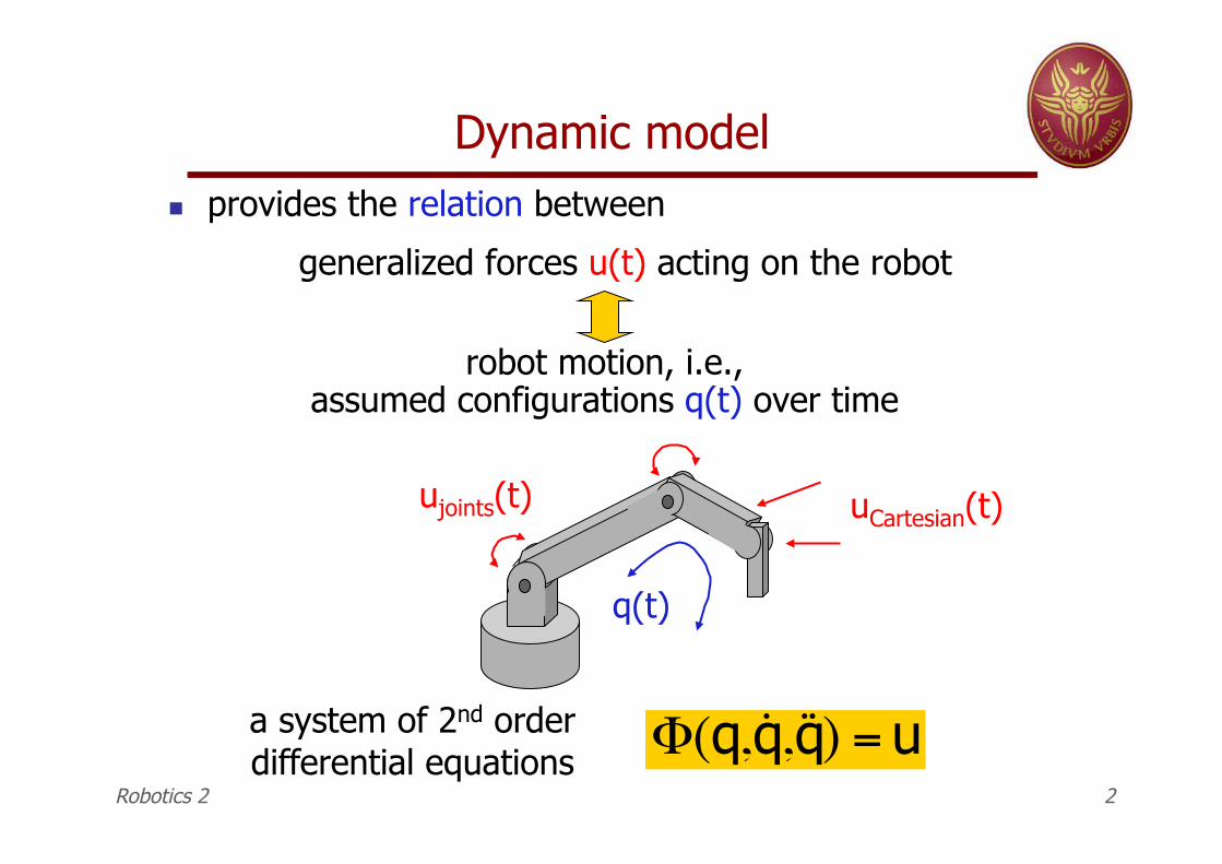
Dynamic model !  provides the relation between

generalized forces u(t) acting on the robot

robot motion, i.e., assumed configurations q(t) over time

!

"(q, ˙ q ,˙ ̇ q ) = u

ujoints(t) uCartesian(t)

q(t)

a system of 2nd order differential equations

Robotics 2 2

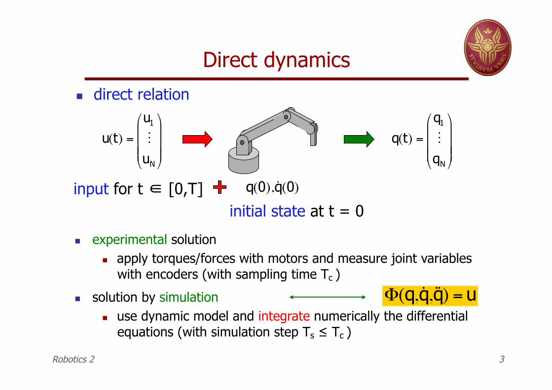
Direct dynamics

!  direct relation

!

u(t) =

u1

!uN

"

#

$ $ $

%

&

' ' '

!

q(t) =

q1

!qN

"

#

$ $ $

%

&

' ' '

!

q(0), ˙ q (0)input for t ∈ [0,T] initial state at t = 0

!  experimental solution !  apply torques/forces with motors and measure joint variables

with encoders (with sampling time Tc )

!  solution by simulation !  use dynamic model and integrate numerically the differential

equations (with simulation step Ts ! Tc )

!

"(q, ˙ q ,˙ ̇ q ) = u

Robotics 2 3

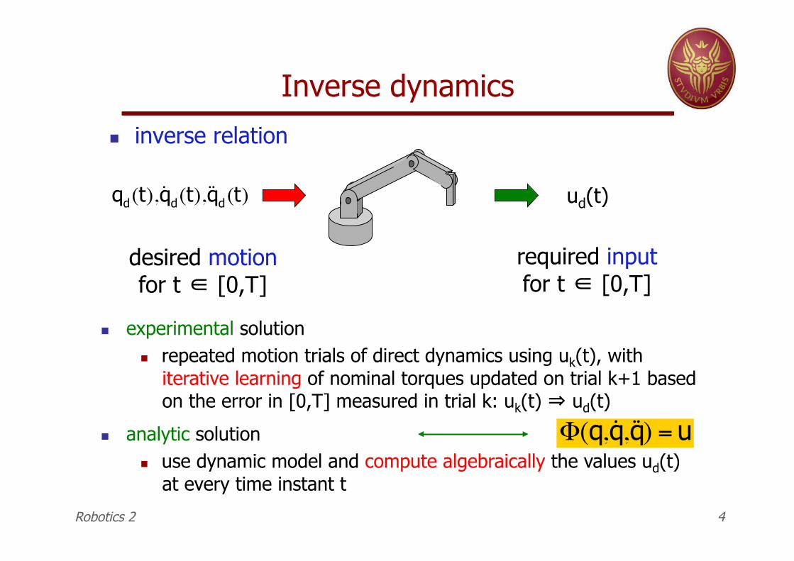
Inverse dynamics

!  inverse relation

desired motion for t ∈ [0,T]

!  experimental solution !  repeated motion trials of direct dynamics using uk(t), with

iterative learning of nominal torques updated on trial k+1 based on the error in [0,T] measured in trial k: uk(t) ⇒ ud(t)

!  analytic solution !  use dynamic model and compute algebraically the values ud(t)

at every time instant t

!

qd(t), ˙ q d(t),˙ ̇ q d(t) ud(t)

required input for t ∈ [0,T]

!

"(q, ˙ q ,˙ ̇ q ) = u

Robotics 2 4

Approaches to dynamic modeling

Euler-Lagrange method (energy-based approach)

!  dynamic equations in symbolic/closed form

!  best for study of dynamic properties and analysis of control schemes

Newton-Euler method (balance of forces/torques)

!  dynamic equations in numeric/recursive form

!  best for implementation of control schemes (inverse dynamics in real time)

"  many formal methods based on basic principles in mechanics are available for the derivation of the robot dynamic model:

"  principle of d’Alembert, of Hamilton, of virtual works, …

Robotics 2 5

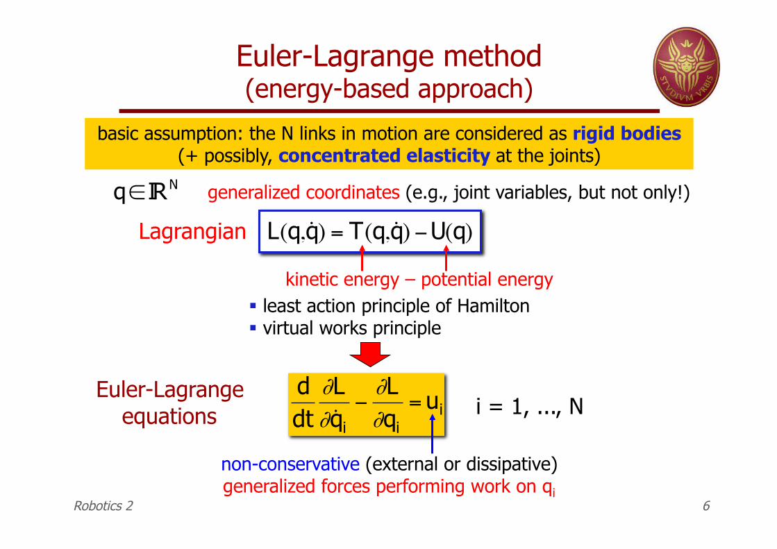
Euler-Lagrange method (energy-based approach)

!

q" IRN

!

ddt

"L" ˙ q i

#"L"qi

= ui

basic assumption: the N links in motion are considered as rigid bodies (+ possibly, concentrated elasticity at the joints)

"  least action principle of Hamilton "  virtual works principle

i = 1, ..., N

non-conservative (external or dissipative) generalized forces performing work on qi

generalized coordinates (e.g., joint variables, but not only!)

Lagrangian

!

L(q, ˙ q ) = T(q, ˙ q ) "U(q)

kinetic energy – potential energy

Euler-Lagrange equations

Robotics 2 6

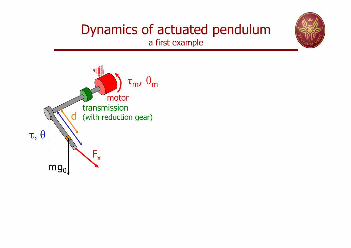
Dynamics of actuated pendulum a first example

!m, "m

!, "

m g0

d

motor transmission (with reduction gear)

Fx

viscous friction bm

b!

!

!

!

T =12

I ! + md2 + n2Im( ) ˙ " 2 =12

I ˙ " 2kinetic energy

!

˙ " m = n ˙ "

!

"m = n"+ "m0= 0

!

q = "

!

T = Tm + T!

!

Tm =12

Im˙ " m

2

!

T! =12

I ! + md2( ) ˙ " 2

link inertia (around the z-axis

through its center of mass)

motor inertia (around its

spinning axis)

(or )

!

q = "m

!

" = n"mn " 1

Robotics 2 7

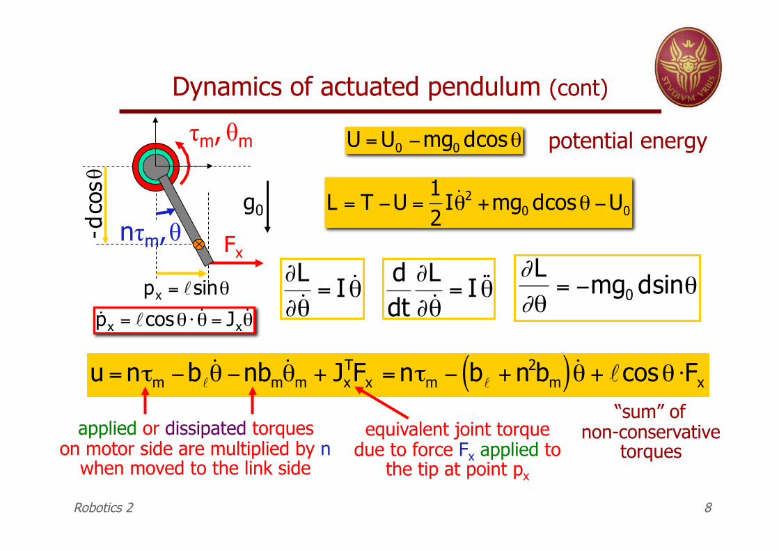
Dynamics of actuated pendulum (cont)

!

U = U0 "mg0 dcos#

n!m, " Fx

- d co

s "

!

L = T "U =12

I ˙ # 2 +mg0 dcos# "U0

!

"L" ˙ #

= I ˙ #

!

ddt"L" ˙ #

= I ˙ ̇ #

!

"L"#

= $mg0 dsin#

!

u = n"m #b! ˙ $ #nbm˙ $ m + Jx

TFx = n"m # b! + n2bm( ) ˙ $ + !cos$ %Fx

!m, "m

!

px = !sin"

!

˙ p x = !cos" # ˙ " = Jx˙ "

potential energy

“sum” of non-conservative

torques applied or dissipated torques

on motor side are multiplied by n when moved to the link side

equivalent joint torque due to force Fx applied to

the tip at point px

Robotics 2 8

g0

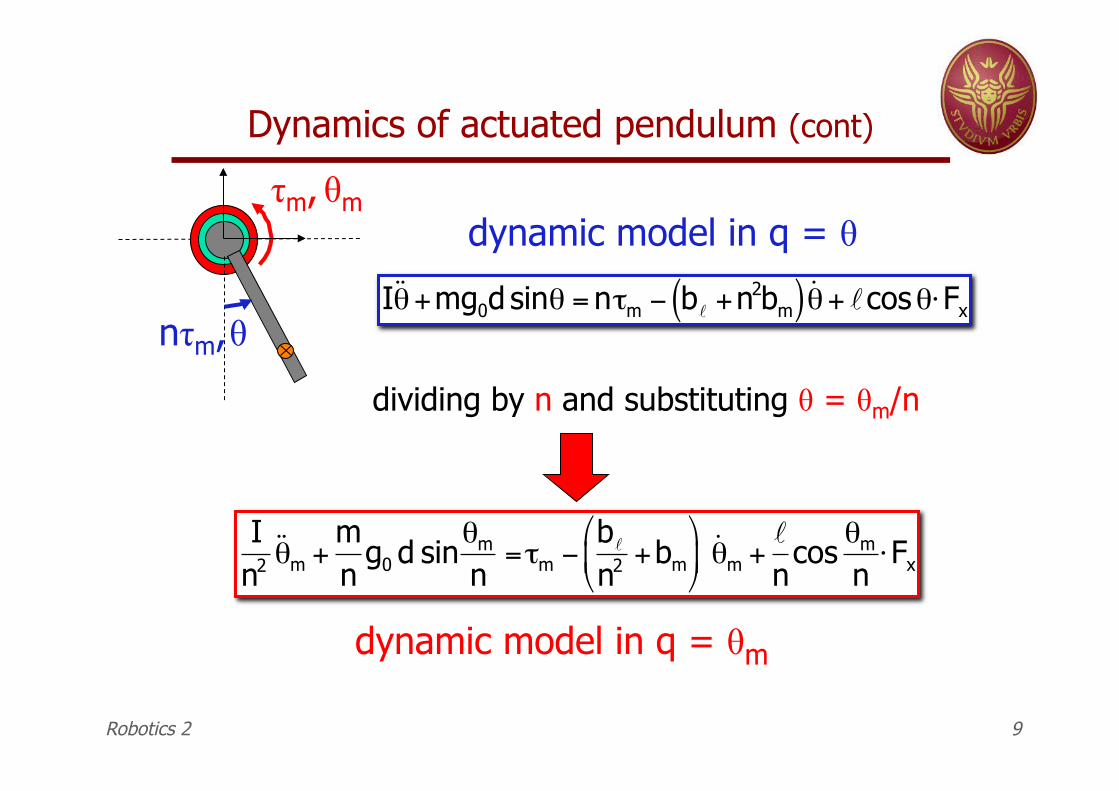
Dynamics of actuated pendulum (cont)

!

In2

˙ ̇ " m +mn

g0 d sin"m

n=#m $

b!n2 +bm

%

& '

(

) * ˙ " m +

!n

cos"m

n+Fx

n!m, "

!m, "m

!

I˙ ̇ " +mg0d sin" = n#m $ b! +n2bm( ) ˙ " + !cos"%Fx

dividing by n and substituting " = "m/n

dynamic model in q = "m

dynamic model in q = "

Robotics 2 9

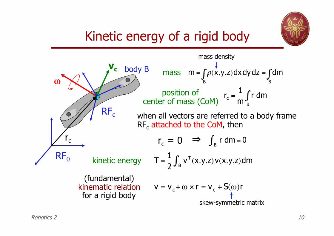
Kinetic energy of a rigid body

RFc

vc

RF0

body B mass

!

m = "(x,y,z)dxdydzB# = dm

B#

mass density

rc

position of center of mass (CoM)

!

rc =1m

r dmB"

when all vectors are referred to a body frame RFc attached to the CoM, then

rc = 0

!

r dmB" = 0⇒

kinetic energy

!

T =12

v T (x,y,z)v(x,y,z)dmB"

(fundamental) kinematic relation for a rigid body

!

v = vc+" # r = vc + S(")r

skew-symmetric matrix

"

Robotics 2 10

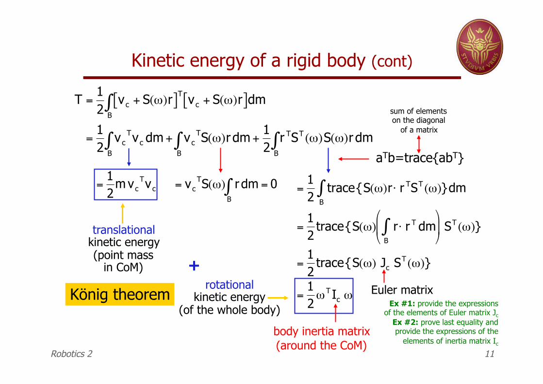
Kinetic energy of a rigid body (cont)

König theorem

!

T =12

vc + S(")r[ ]T vc + S(")r[ ]dmB#

=12

vcTvc dm

B# + vc

TS(")r dmB# +

12

r TST (")S(")r dmB#

!

= vcTS(") r dm

B# = 0

!

=12

m vcTvc

!

=12

trace{S(")r# r TST (")}dmB$

=12

trace{S(") r# r T dmB$

%

& '

(

) * ST (")}

=12

trace{S(") Jc ST (")}

=12" T Ic "

aTb=trace{abT}

sum of elements on the diagonal

of a matrix

Euler matrix

translational kinetic energy (point mass

in CoM) rotational

kinetic energy (of the whole body)

body inertia matrix (around the CoM)

+

Robotics 2 11

Ex #1: provide the expressions of the elements of Euler matrix Jc

Ex #2: prove last equality and provide the expressions of the

elements of inertia matrix Ic

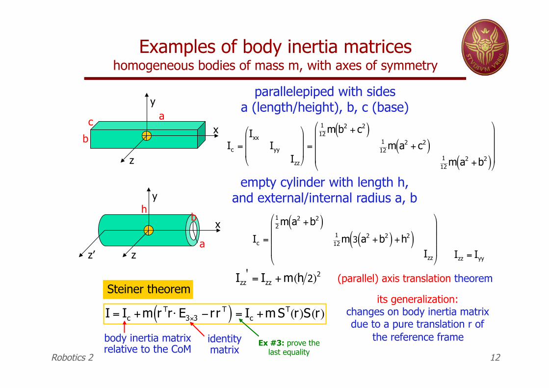
Examples of body inertia matrices homogeneous bodies of mass m, with axes of symmetry

parallelepiped with sides a (length/height), b, c (base)

!

Ic =Ixx

Iyy

Izz

"

#

$ $

%

&

' ' =

112 m b2 + c2( )

112 m a2 + c2( )

112 m a2 +b2( )

"

#

$ $ $

%

&

' ' '

x

y

z

b

c a

!

Ic =

12 m a2 +b2( )

112 m 3 a2 +b2( ) +h2( )

Izz

"

#

$ $ $

%

&

' ' '

empty cylinder with length h, and external/internal radius a, b

x

y

z a

h b

z’

!

Izz = Iyy

!

Izz' = Izz + m(h 2)2 (parallel) axis translation theorem

!

I = Ic +m r Tr" E3#3 $ rr T( ) = Ic +m ST(r)S(r)its generalization:

changes on body inertia matrix due to a pure translation r of

the reference frame body inertia matrix relative to the CoM

identity matrix

Steiner theorem

Robotics 2 12

Ex #3: prove the last equality

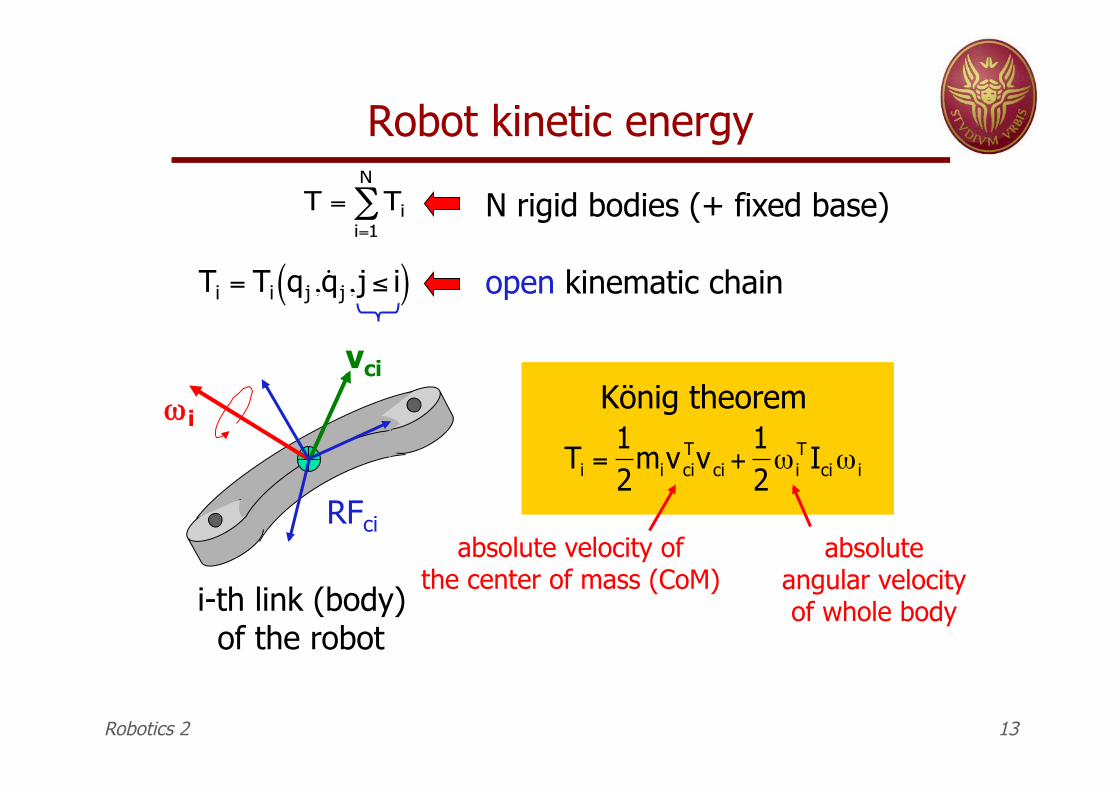
Robot kinetic energy

!

T = Tii=1

N

"

!

Ti = Ti qj , ˙ q j , j " i( )

!

Ti =12

mivciTvci +

12" i

T Ici" i

N rigid bodies (+ fixed base)

open kinematic chain

König theorem

absolute velocity of the center of mass (CoM)

absolute angular velocity of whole body

RFci

vci

i-th link (body) of the robot

i "

Robotics 2 13

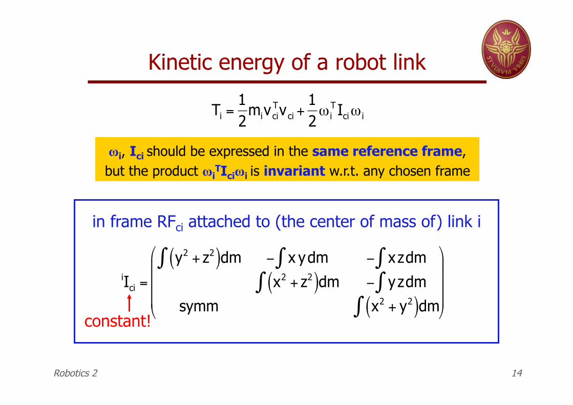
Kinetic energy of a robot link

!

iIci =

y2 + z2( )dm" # x ydm" # xzdm"x2 + z2( )dm" # yzdm"

symm x2 + y2( )dm"

$

%

& & &

'

(

) ) )

!i, Ici should be expressed in the same reference frame, but the product !i

TIci!i is invariant w.r.t. any chosen frame

in frame RFci attached to (the center of mass of) link i

constant!

Robotics 2 14

!

Ti =12

mivciTvci +

12" i

T Ici" i

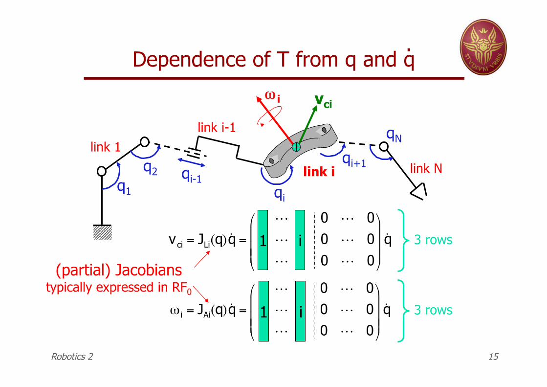
Dependence of T from q and q

q1

link 1

qi-1 qi

qN link i-1

link N link i q2

vci

qi+1

!

vci = JLi(q) ˙ q =! 0 ! 0! 0 ! 0! 0 ! 0

"

#

$ $ $

%

&

' ' '

˙ q i 1

!

" i = JAi(q) ˙ q =! 0 ! 0! 0 ! 0! 0 ! 0

#

$

% % %

&

'

( ( (

˙ q i 1

3 rows

3 rows

.

(partial) Jacobians typically expressed in RF0

" i

Robotics 2 15

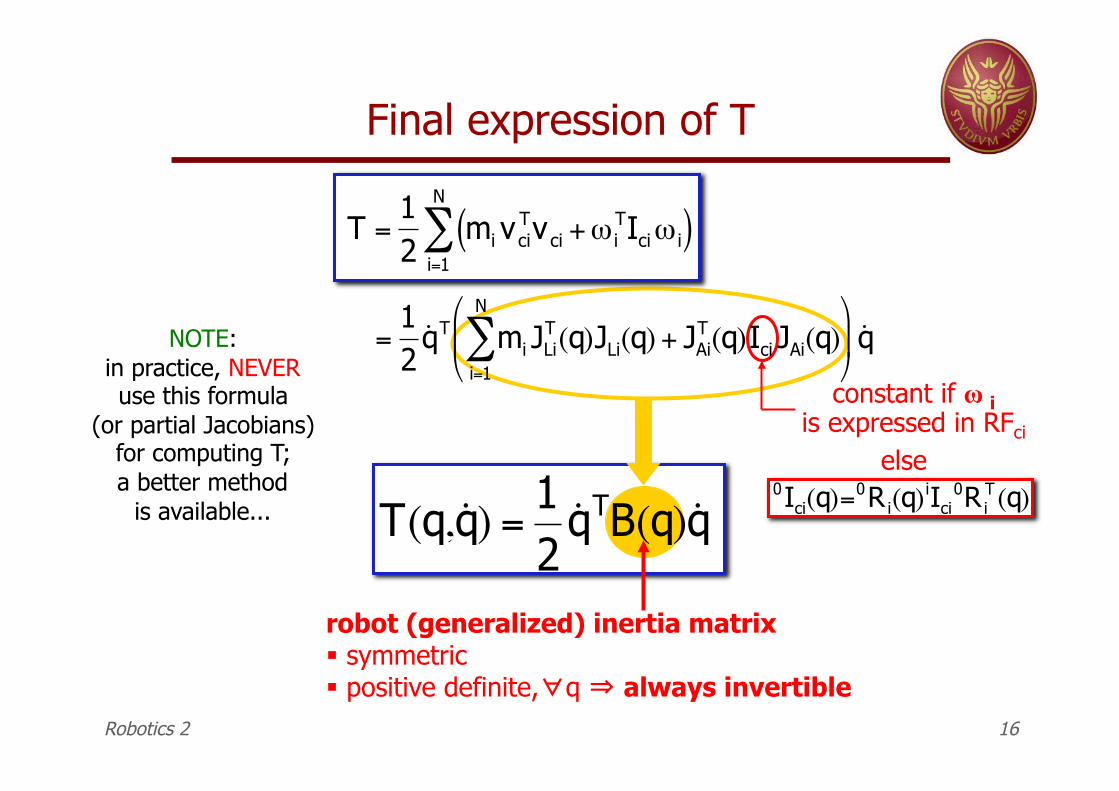
Final expression of T

!

T =12

mi vciTvci +" i

TIci" i( )i=1

N

#

!

=12

˙ q T mi JLiT (q)JLi(q) + JAi

T (q)Ici JAi(q)i=1

N

"#

$ %

&

' ( ˙ q

robot (generalized) inertia matrix "  symmetric "  positive definite,∀q ⇒ always invertible

constant if ! i is expressed in RFci

!

T(q, ˙ q ) =12

˙ q TB(q) ˙ q else

!

0Ici(q)=0Ri(q)

iIci0R i

T (q)

NOTE: in practice, NEVER use this formula

(or partial Jacobians) for computing T; a better method

is available...

Robotics 2 16

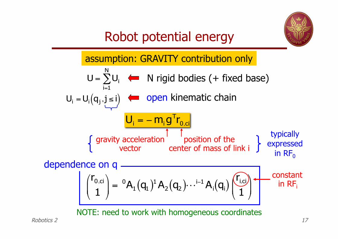
Robot potential energy

!

U = Uii=1

N

"

!

Ui = Ui qj , j " i( )

assumption: GRAVITY contribution only

!

Ui = "migTr0,ci

gravity acceleration vector

position of the center of mass of link i

typically expressed

in RF0

!

r0,ci

1"

# $

%

& ' =

0A1 q1( )1 A2 q2( )!i(1 Ai qi( )ri,ci

1"

# $

%

& '

dependence on q constant

in RFi

NOTE: need to work with homogeneous coordinates

N rigid bodies (+ fixed base)

open kinematic chain

Robotics 2 17

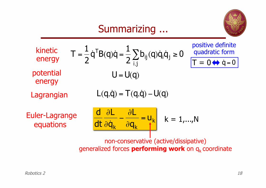
Summarizing ...

!

T =12

˙ q TB(q) ˙ q = 12

bij (q) ˙ q i ˙ q ji,j" # 0

!

L(q, ˙ q ) = T(q, ˙ q ) "U(q)

!

U = U(q)

!

ddt

"L" ˙ q k

#"L"qk

= uk k = 1,...,N

T = 0

!

˙ q = 0

positive definite quadratic form kinetic

energy

potential energy

Lagrangian

Euler-Lagrange equations

non-conservative (active/dissipative) generalized forces performing work on qk coordinate

Robotics 2 18

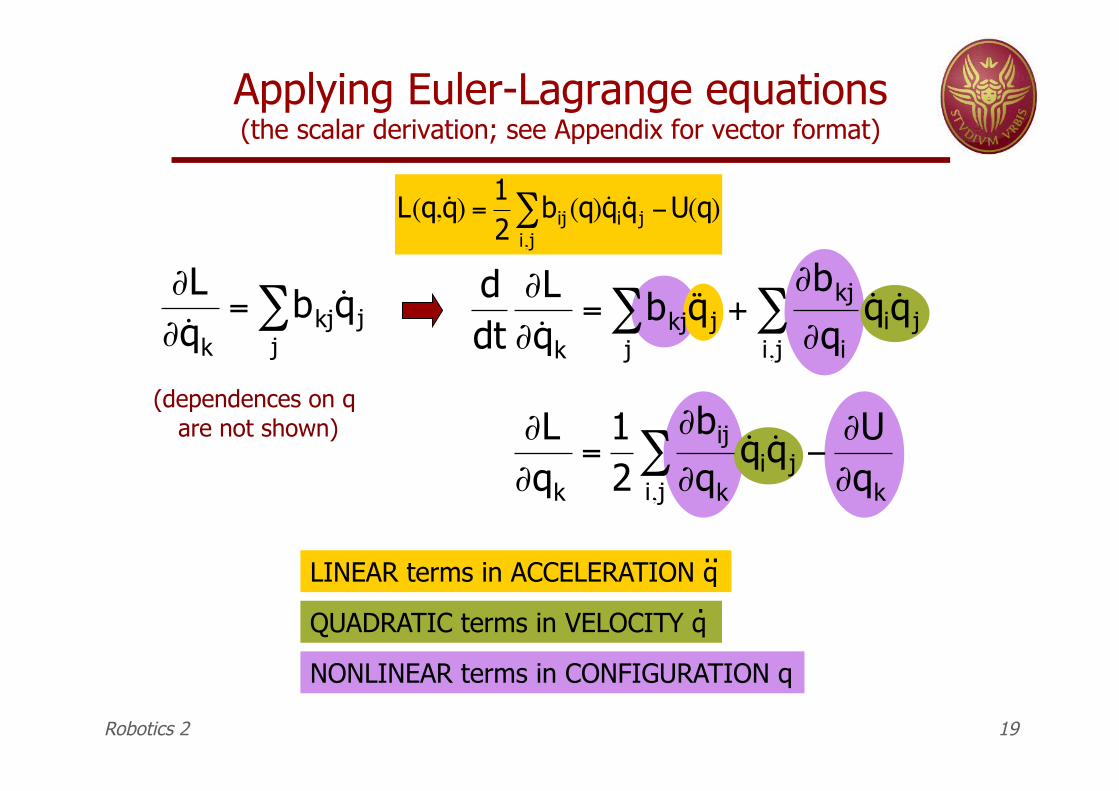
Applying Euler-Lagrange equations (the scalar derivation; see Appendix for vector format)

!

"L" ˙ q k

= bkj ˙ q jj#

!

ddt

"L" ˙ q k

= bkj˙ ̇ q jj# +

"bkj

"qi

˙ q i ˙ q ji,j#

!

"L"qk

=12

"bij

"qk

˙ q i ˙ q ji,j# $

"U"qk

NONLINEAR terms in CONFIGURATION q

LINEAR terms in ACCELERATION q ..

QUADRATIC terms in VELOCITY q .

(dependences on q are not shown)

!

L(q, ˙ q ) =12

bij (q) ˙ q i ˙ q ji,j" #U(q)

Robotics 2 19

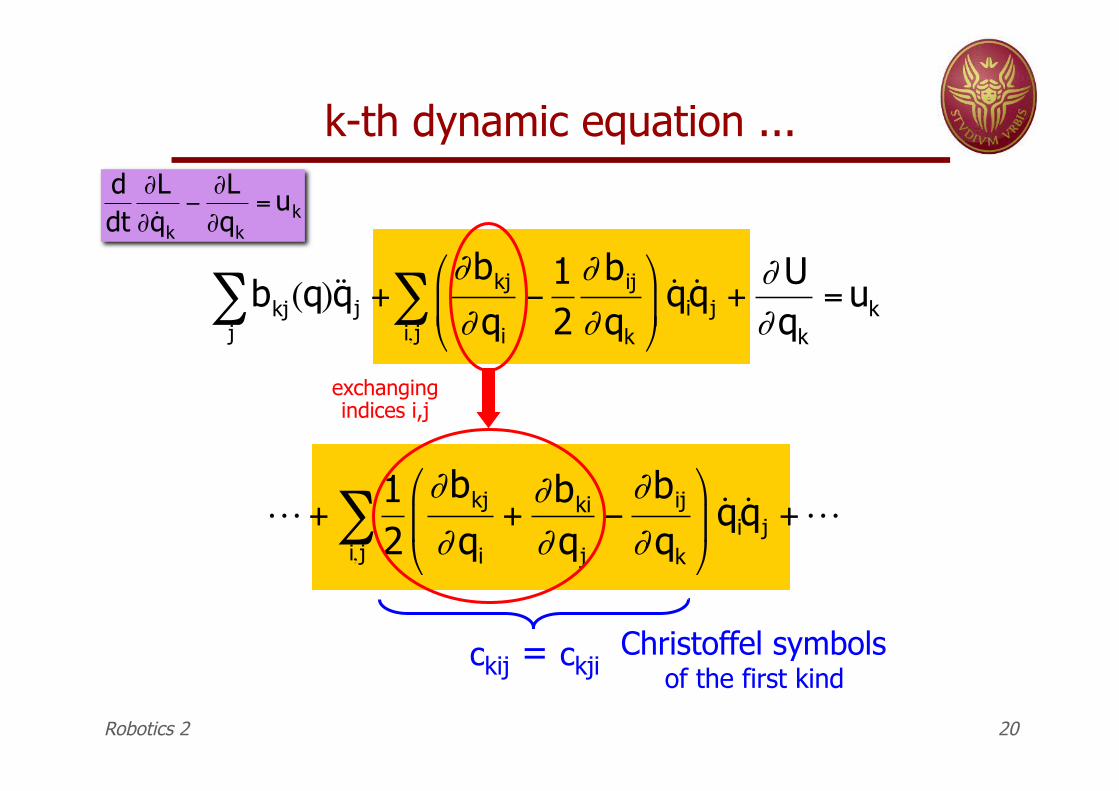
k-th dynamic equation ...

!

bkj(q)˙ ̇ q j +j"

#bkj

#qi

$12# bij

#qk

%

& '

(

) * ˙ q i˙ q j

i, j" +

#U#qk

= uk

!

! +12"bkj

"qi

+"bki

"qj

#"bij

"qk

$

% &

'

( ) ˙ q i˙ q j

i, j* +!

ckij = ckji Christoffel symbols

of the first kind

!

ddt

"L" ˙ q k

#"L"qk

= uk

exchanging indices i,j

Robotics 2 20

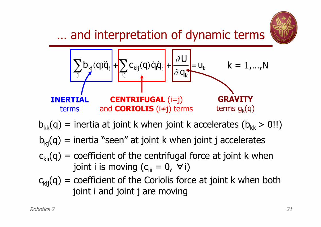
… and interpretation of dynamic terms

!

bkj(q)˙ ̇ q j +j" ckij(q) ˙ q i˙ q j

i, j" +

#U# qk

= uk

INERTIAL terms

CENTRIFUGAL (i=j) and CORIOLIS (i#j) terms

GRAVITY terms gk(q)

k = 1,…,N

bkj(q) = inertia “seen” at joint k when joint j accelerates

ckij(q) = coefficient of the Coriolis force at joint k when both joint i and joint j are moving

bkk(q) = inertia at joint k when joint k accelerates (bkk > 0!!)

ckii(q) = coefficient of the centrifugal force at joint k when joint i is moving (ciii = 0, ∀i)

Robotics 2 21

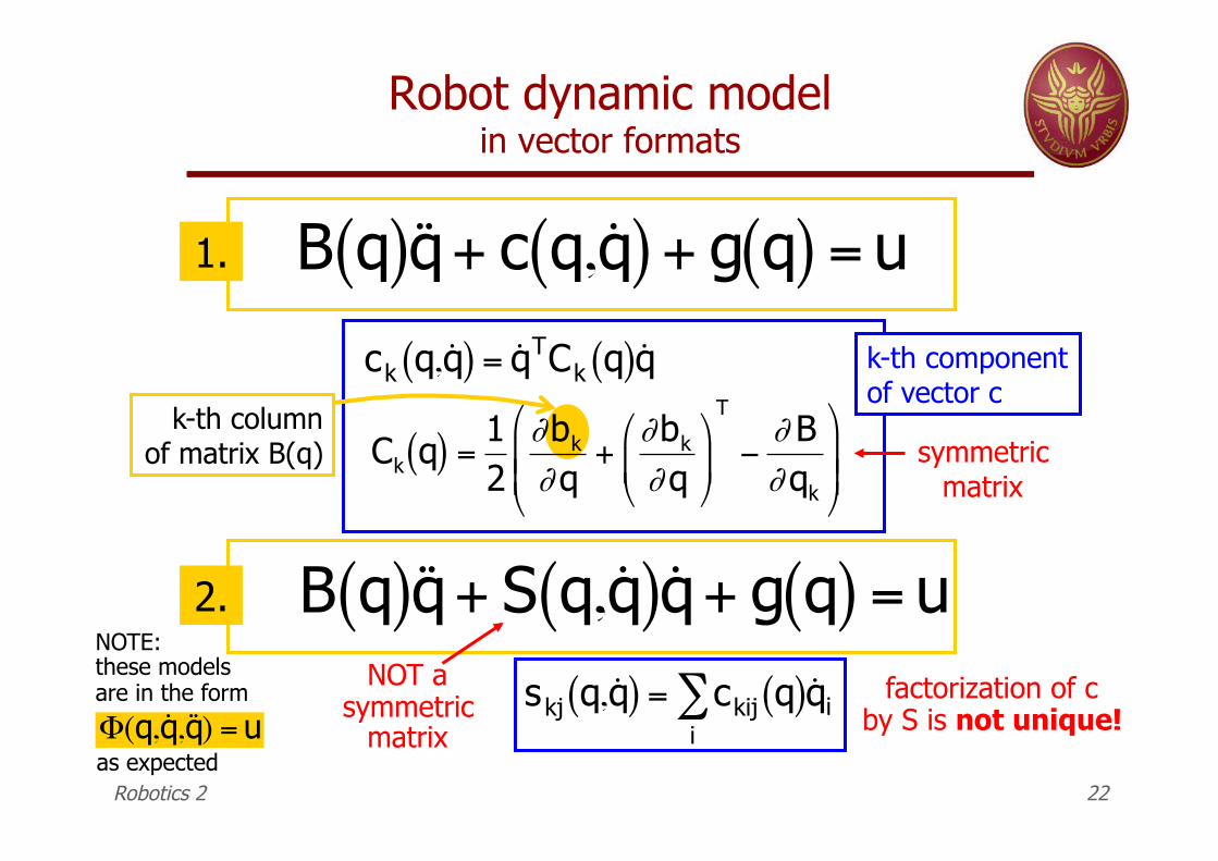
Robot dynamic model in vector formats

!

B q( )˙ ̇ q + c q, ˙ q ( ) + g q( ) = u

!

ck q, ˙ q ( ) = ˙ q TCk q( ) ˙ q

!

Ck q( ) =12

"bk

"q+

"bk

"q#

$ %

&

' (

T

)"B"qk

#

$ % %

&

' ( (

!

B q( )˙ ̇ q + S q, ˙ q ( )˙ q + g q( ) = u

!

skj q, ˙ q ( ) = ckij q( )˙ q ii"

k-th component of vector c

k-th column of matrix B(q) symmetric

matrix

NOT a symmetric

matrix

1.

2.

factorization of c by S is not unique!

!

"(q, ˙ q ,˙ ̇ q ) = u

NOTE: these models are in the form

as expected Robotics 2 22

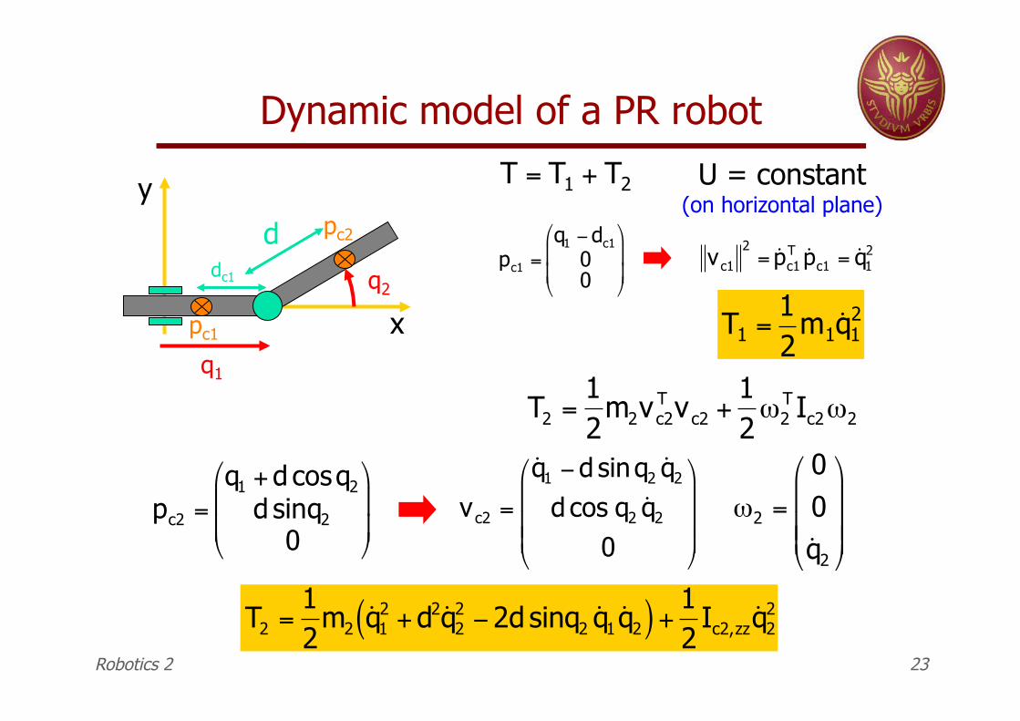
Dynamic model of a PR robot

q1

q2

x

y

!

T1 =12

m1 ˙ q 12

!

T2 =12

m2vc2T vc2 +

12"2

T Ic2"2

pc2

!

pc2 =q1 + d cosq2

d sinq20

"

#

$ $

%

&

' '

!

vc2 =

˙ q 1 "d sinq2˙ q 2

d cos q2˙ q 2

0

#

$

% % %

&

'

( ( (

!

"2 =

00˙ q 2

#

$

% % %

&

'

( ( (

!

T2 =12

m2˙ q 1

2 + d2˙ q 22 "2d sinq2

˙ q 1 ˙ q 2( ) +12

Ic2,zz˙ q 2

2

!

T = T1 + T2 U = constant (on horizontal plane)

Robotics 2 23

d dc1

!

pc1 =q1 "dc1

00

#

$

% %

&

'

( (

!

vc12

= ˙ p c1T ˙ p c1 = ˙ q 1

2

pc1

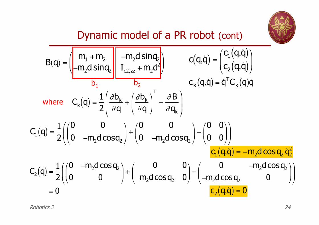
Dynamic model of a PR robot (cont)

!

B(q) =m1 +m2 "m2d sinq2

"m2d sinq2 Ic2,zz +m2d2

#

$ %

&

' (

b1 b2

!

ck q, ˙ q ( ) = ˙ q TCk q( ) ˙ q

!

c q, ˙ q ( ) =c1 q, ˙ q ( )c2 q, ˙ q ( )"

# $

%

& '

where

!

C1 q( ) =12

0 00 "m2d cosq2

#

$ %

&

' ( +

0 00 "m2d cosq2

#

$ %

&

' ( "

0 00 0#

$ %

&

' (

#

$ %

&

' (

!

c1 q, ˙ q ( ) = "m2d cosq2˙ q 2

2

!

Ck q( ) =12

"bk

"q+

"bk

"q#

$ %

&

' (

T

)"B"qk

#

$ % %

&

' ( (

!

C2 q( ) =12

0 "m2d cosq2

0 0#

$ %

&

' ( +

0 0"m2d cosq2 0#

$ %

&

' ( "

0 "m2d cosq2

"m2d cosq2 0#

$ %

&

' (

#

$ %

&

' (

= 0

!

c2 q, ˙ q ( ) = 0

Robotics 2 24

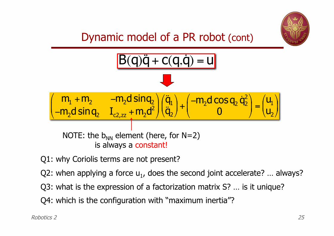
Dynamic model of a PR robot (cont)

!

m1 +m2 "m2d sinq2

"m2d sinq2 Ic2,zz +m2d2

#

$ %

&

' (

˙ ̇ q 1˙ ̇ q 2# $ %

& ' ( + "m2d cosq2

˙ q 22

0#

$ %

&

' ( =

u1u2

# $ %

& ' (

!

B(q)˙ ̇ q + c(q, ˙ q ) = u

NOTE: the bNN element (here, for N=2) is always a constant!

Q4: which is the configuration with “maximum inertia”?

Q1: why Coriolis terms are not present?

Q2: when applying a force u1, does the second joint accelerate? … always?

Q3: what is the expression of a factorization matrix S? … is it unique?

Robotics 2 25

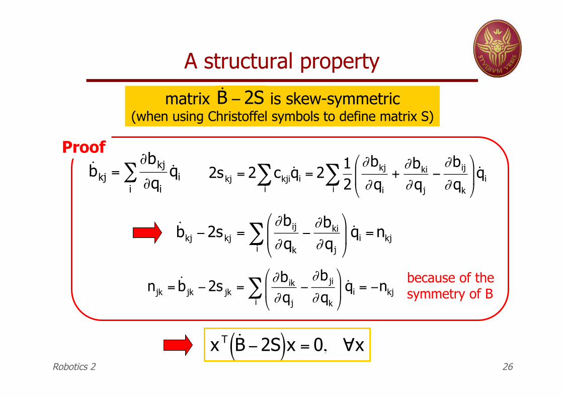
A structural property

matrix is skew-symmetric (when using Christoffel symbols to define matrix S)

!

˙ B " 2S

!

˙ b kj ="bkj

"qi

˙ q ii#

!

2skj = 2 ckji˙ q i

i" = 2

12#bkj

#qi

+#bki

#qj

$#bij

#qk

%

& '

(

) * ̇ q i

i"

!

˙ b kj "2skj =#bij

#qk

"#bki

#qj

$

% &

'

( ) ˙ q i = nkj

i*

!

njk = ˙ b jk "2s jk =#bik

#qj

"#bji

#qk

$

% &

'

( ) ˙ q i = "nkj

i*

Proof

because of the symmetry of B

!

x T ˙ B "2S( )x = 0, #xRobotics 2 26

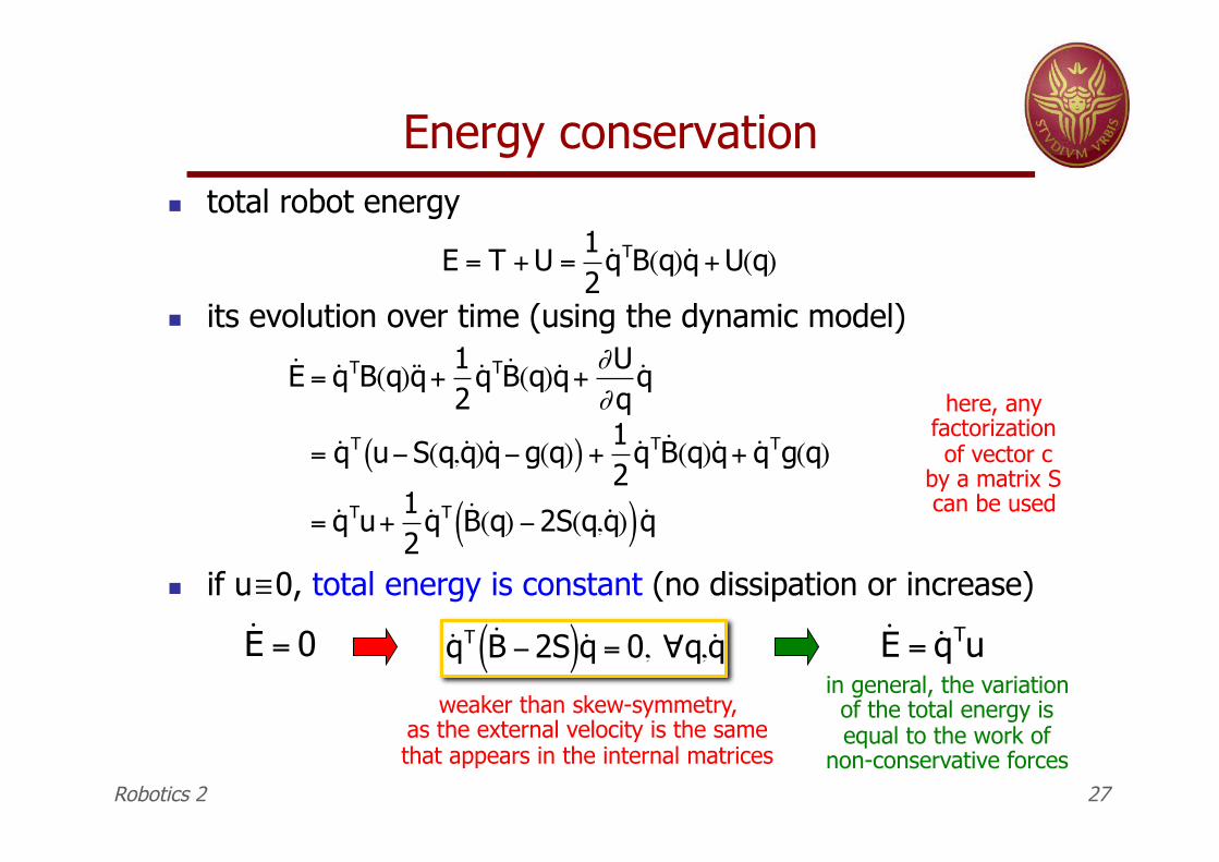
!  total robot energy

!  its evolution over time (using the dynamic model)

!  if u≡0, total energy is constant (no dissipation or increase)

Energy conservation

!

E = T + U =12

˙ q TB(q)˙ q + U(q)

!

˙ q T ˙ B "2S( )˙ q = 0, #q, ˙ q

here, any factorization of vector c

by a matrix S can be used

!

˙ E = ˙ q TB(q)˙ ̇ q + 12

˙ q T ˙ B (q)˙ q + "U"q

˙ q

= ˙ q T u#S(q, ˙ q )˙ q #g(q)( ) +12

˙ q T ˙ B (q)˙ q + ˙ q Tg(q)

= ˙ q Tu+12

˙ q T ˙ B (q) #2S(q, ˙ q )( ) ˙ q

!

˙ E = ˙ q Tu

!

˙ E = 0

weaker than skew-symmetry, as the external velocity is the same that appears in the internal matrices

in general, the variation of the total energy is equal to the work of

non-conservative forces Robotics 2 27

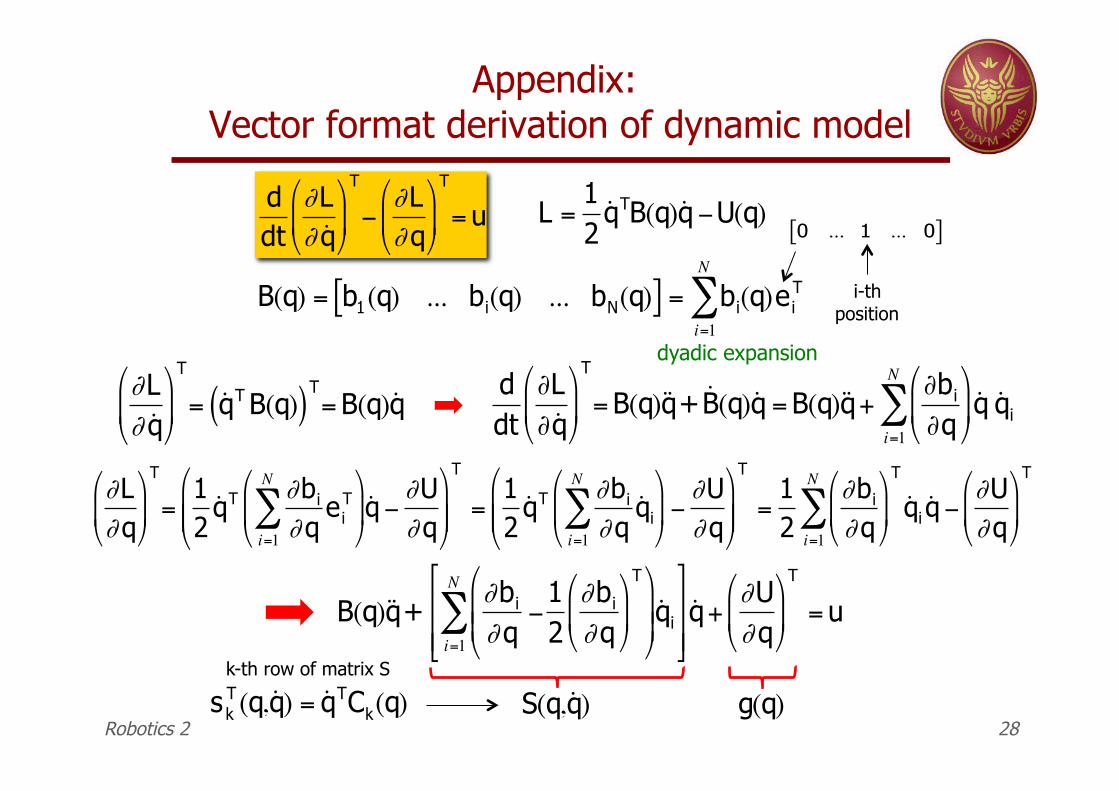
Appendix: Vector format derivation of dynamic model

Robotics 2 28

!

L =12

˙ q TB(q)˙ q "U(q)

!

ddt

"L" ˙ q

#

$ %

&

' (

T

)"L"q

#

$ %

&

' (

T

= u

!

B(q) = b1(q) ... bi(q) ... bN(q)[ ] = bi(q)eiT

i=1

N

"

!

0 ... 1 ... 0[ ]

i-th position

dyadic expansion

!

"L" ˙ q

#

$ %

&

' (

T

= ˙ q T B(q)( )T= B(q)˙ q

!

"L"q

#

$ %

&

' (

T

=12

˙ q T"bi

"qei

T

i=1

N

)#

$ %

&

' ( ̇ q *

"U"q

#

$ % %

&

' ( (

T

=12

˙ q T"bi

"q˙ q i

i=1

N

)#

$ %

&

' ( *

"U"q

#

$ % %

&

' ( (

T

=12

"bi

"q

#

$ %

&

' (

T

˙ q ii=1

N

) ˙ q *"U"q

#

$ %

&

' (

T

!

ddt

"L" ˙ q

#

$ %

&

' (

T

= B(q)˙ ̇ q + ˙ B (q)˙ q = B(q)˙ ̇ q +"bi

"q

#

$ %

&

' ( ̇ q

i=1

N

) ˙ q i

!

B(q)˙ ̇ q +"bi

"q#

12"bi

"q

$

% &

'

( )

T$

% & &

'

( ) ) ̇ q i

i=1

N

*+

, - -

.

/ 0 0

˙ q +"U"q

$

% &

'

( )

T

= u

!

skT (q, ˙ q ) = ˙ q TCk(q)k-th row of matrix S

!

g(q)

!

S(q, ˙ q )