Prof Bill Hillier - Royal Institute of Technology/Menu/general/column... · Prof Bill Hillier University of London, UK May 20, 2010 Seminar: Security Matters! ... Logistic Model Coefficients

Crime and urban design

Prof Bill Hillier University of London, UKUniversity of London, UK

May 20, 2010

Seminar: Security Matters! Stockholm, May 20-21

SafeScape

Defensible Space

Public vs. Private

Maximize commons to promote interaction and a sense of community

Maximize private areas to create defensibl e space; create a sense of community throu gh smaller developments with fewer strangers

Uses

Mix uses to p rovi de activi ty and increase eyes on the street

Mixed use reduces residential control and therefore increases crime

Streets and Footpaths

Encourage walki ng and cycling, increase surveill ance through a grid street pat tern

Limit access and escape opp ortun it ies to provi de more privacy and increase residential control

All eys Face buildi ngs toward al leys to provi de El iminate or gate al leys as they increase

• .

All eys

Face buildi ngs toward al leys to provi de eyes on the alley

El iminate or gate al leys as they increase burglary and are dangerous for pedes trian s

Autos

Build homes close to t he street , forcing parking to be on the street or in rear courtyards

Autos are safest in garages or visible in front of the house; rear courtyards facili tate burglary

Density High density to promote act ivi ty,

sustain publi c trans it, and reduce sprawl

Dens ity creates vulnerabil ity when it increases common areas or unsafe parking

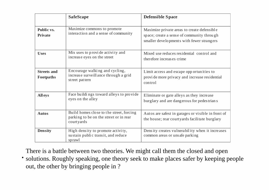
There is a battle between two theories. We might call them the closed and open solutions. Roughly speaking, one theory seek to make places safer by keeping people out, the other by bringing people in ?

The key design-crime questions for residential burglary

• - Are some kinds of dwellings safer than others ?

• - Is density good or bad ?

• - Is movement in your street good or bad ?

• - Does it matter how we group dwellings ?

• - Are cul de sacs safe or unsafe ?

• - Is mixed use beneficial or not ?

• - Should residential areas be permeable or impermeable ?

• - Do social factors make a difference ?

https://www.ipam.ucla.edu/publications/chs2007/chs2007_6801.ppt

• The study reported here is of 5 years of all the police crime data in a London borough made up of:

– A population of 263000

– 101849 dwellings in 65459 residential buildings

– 536 kilometres of road, made up of 7102 street segments

– Many centres and sub-centres at different scales

– Over 13000 burglaries

– Over 6000 street robberies

• We are focusing our study on residential burglary and street robbery as these are the two crimes that people most fear today.

• Residential burglary and street robbery data tables have been created at several levels:

– the 21 Wards (around 12000 people) that make up the borough for average residential burglary and street robbery rates. At this level, spatial data is numerically accurate, but reflects only broad spatial characteristics of areas. Social data from the 2001 Census is available, including ‘deprivation index’, but at this level patterns are broad and scene-setting at best.

– the 800 Output Areas (around 125 dwellings) from the 2001 Census, so social data is rich and includes full demographic, occupation, social deprivation, unemployment, population and housing densities, and ethnic deprivation, unemployment, population and housing densities, and ethnic mix, as well as houses types and forms of tenure. Unfortunately spatial data is fairly meaningless at this level due to the arbitrary shape of Output Areas.

– the 7102 street segments (between intersections) that make up the borough. Here we have optimal spatial data, good physical data and ‘council tax band’ data indicating property values which can act as a surrogate for social data

– Finally, the 65459 individual residential buildings, comprising 101849 dwellings. Here spatial values are taken from the associated segment, and again we have good physical data with Council Tax band as social surrogate. Street robbery cannot of course be assigned here.

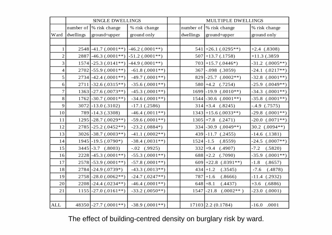
number of % risk change % risk change number of % risk change % risk change

Ward dwellings ground+upper ground only dwellings ground+upper ground only

1 2548 -41.7 (.0001**) -46.2 (.0001**) 541 +26.1 (.0295**) +2.4 (.8308)

2 2887 -46.3 (.0001**) -51.2 (.0001**) 507 +13.7 (.1758) +11.3 (.3859

3 1574 -25.3 (.0141**) -44.9 (.0001**) 703 +15.7 (.0446*) -31.2 (.0005**)

4 2702 -55.9 (.0001**) -61.8 (.0001**) 367 -.098 (.3059) -24.1 (.0217**)

5 2734 -42.4 (.0001**) -49.7 (.0001**) 829 -25.7 (.0002**) -32.8 (.0001**)

6 2711 -32.6 (.0315**) -35.6 (.0001**) 580 +4.2 (.7254) -25.9 (.0049**)

7 1363 -27.6 (.0073**) -45.3 (.0001**) 1699 -19.9 (.0010**) -34.3 (.0001**)

8 1762 -30.7 (.0001**) -34.6 (.0001**) 1544 -30.6 (.0001**) -35.8 (.0001**)

9 3072 -13.0 (.3102) -17.1 (.2586) 314 +3.4 (.8245) -.4.9 (.7575)

10 789 -14.3 (.3308) -46.4 (.0011**) 1343 +15.6 (.0033**) -29.8 (.0001**)

11 1295 -28.7 (.0029**) -59.6 (.0001**) 1305 +7.8 (.2471) -20.0 (.0071**)

SINGLE DWELLINGS MULTIPLE DWELLINGS

11 1295 -28.7 (.0029**) -59.6 (.0001**) 1305 +7.8 (.2471) -20.0 (.0071**)

12 2785 -25.2 (.0452**) -23.2 (.0884*) 334 -30.9 (.0049**) 30.2 (.0094**)

13 3026 -38.7 (.0003**) -41.1 (.0002**) 439 -11.7 (.2455) -14.6 (.1381)

14 1945 -19.5 (.0790*) -38.4 (.0031**) 1524 -1.5 (.8559) -24.5 (.0007**)

15 3445 -3.7 (.8003) -.02 (.9925) 332 +9.4 (.4907) -7.2 (.5820)

16 2228 -45.3 (.0001**) -55.3 (.0001**) 688 +2.2 (.7090) -35.9 (.0001**)

17 2578 -53.9 (.0001**) -57.8 (.0001**) 609 +22.8 (.0391**) -1.8 (.8657)

18 2784 -24.9 (.0739*) -43.3 (.0013**) 434 +1.2 (.3545) -7.6 (.4878)

19 2758 -28.0 (.0062**) -24.7 (.0247**) 787 +1.6 (.8666) -11.4 (.2932)

20 2208 -24.4 (.0234**) -46.4 (.0001**) 648 +8.1 (.4437) +3.6 (.6886)

21 1155 -27.0 (.0161**) -33.2 (.0050**) 1547 -21.8 (.0002** ) -23.0 (.0001)

ALL 48350 -27.7 (.0001**) -38.9 (.0001**) 17103 2.2 (0.1784) -16.0 .0001

The effect of building-centred density on burglary risk by ward.

-1.140 .175 -6.522 42.539 <.0001 .320 .227 .450

.171 .020 8.402 70.596 <.0001 1.187 1.140 1.235

.097 .013 7.237 52.379 <.0001 1.102 1.073 1.131

.003 .001 2.716 7.376 .0066 1.003 1.001 1.005

-.166 .045 -3.681 13.552 .0002 .847 .775 .925

Coef Std. Error Coef/SE Chi-Square P-Value Exp(Coef) 95% Low er 95% Upper

1: constant

TOmovCITYscale

THRUmovCITYscale

Tomov300m

THRUmov300m

Logistic Model Coefficients Table for Burgled_LSplit By: LUandRU=1then1else0Cell: 1.000

-1.139 .233 -4.898 23.990 <.0001 .320 .203 .505

.061 .028 2.192 4.805 .0284 1.063 1.006 1.122

.039 .018 2.222 4.937 .0263 1.040 1.005 1.076

.010 .001 8.276 68.486 <.0001 1.010 1.007 1.012

-.129 .055 -2.347 5.510 .0189 .879 .790 .979


1: constant

TOmovCITYscale

THRUmovCITYscale

Tomov300m

THRUmov300m

Logistic Model Coefficients Table for Burgled_LSplit By: LUandRU=1then1else0Cell: 0.000

-.392 .144 -2.722 7.410 .0065 .676 .509 .896

.225 .016 13.980 195.442 <.0001 1.253 1.214 1.293


1: constant

TOmovCITYscale

Logistic Model Coefficients Table for Burgled_L

.009 .001 10.556 111.427 <.0001 1.009 1.007 1.010

.062 .011 5.824 33.913 <.0001 1.064 1.042 1.087

-.149 .036 -4.157 17.278 <.0001 .862 .804 .925

-.037 .014 -2.607 6.797 .0091 .963 .937 .991

Tomov300m

THRUmovCITYscale

THRUmov300m

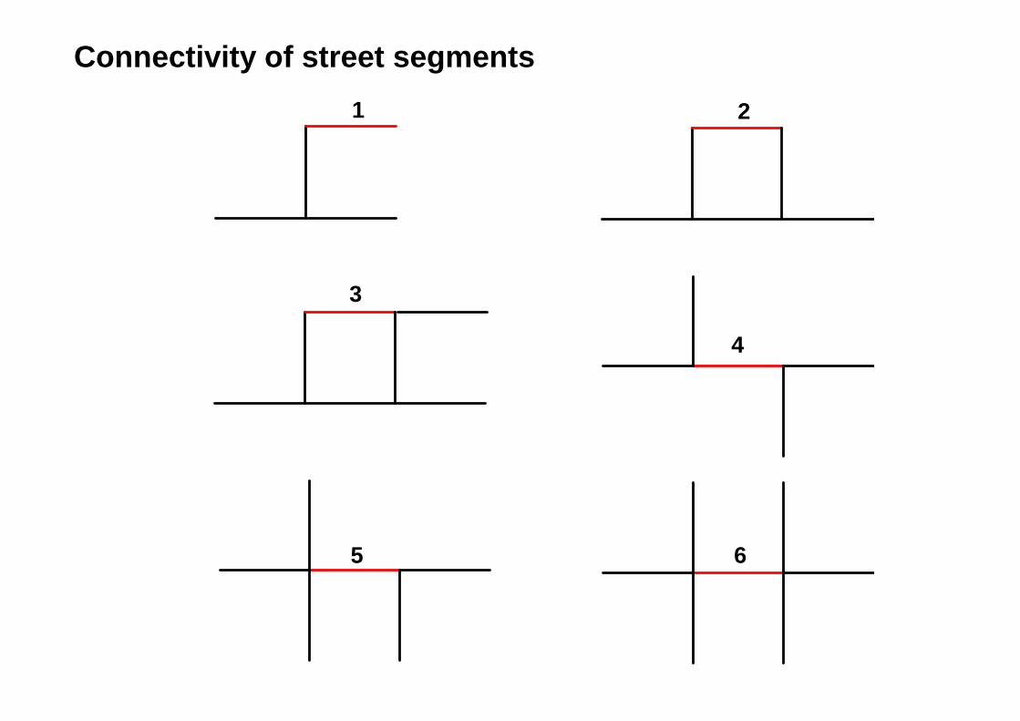
SEGMENTlinks

4

1 2

3

Connectivity of street segments

65

.3

.4

.5

.6

.7

Var

iabl

es

E-band

D-band

C-band

B-band

Univariate Line Chart

segment links from 1-2 to 6

-.1

0

.1

.2

.3

Var

iabl

es

H-band

G-band

F-band

E-band

.25

.28

.3

.32

.35

.38

MA

5BU

RG

/HO

US

EH

OLD

S

MA5BURG/HOUSEHOLDS


number of dwellings per segment

.13

.15

.17

.2

.22

.25

MA

5BU

RG

/HO

US

EH

OLD

S

.25

.3

.35

.4

.45

coun

tBU

RG

/allR

ES

MA

3

Regression Plot

.1

.15

.2

.25

coun

tBU

RG

/allR

ES

MA

3

2.43 2.44 2.45 2.46 2.47 2.48 2.49 2.5 2.51 2.52 2.53INTEGRATIONr14MA3

Y = -1.219 + .565 * X; R^2 = .04

.3

.35

.4

.45co

untB

UR

G/a

llRE

SM

A3

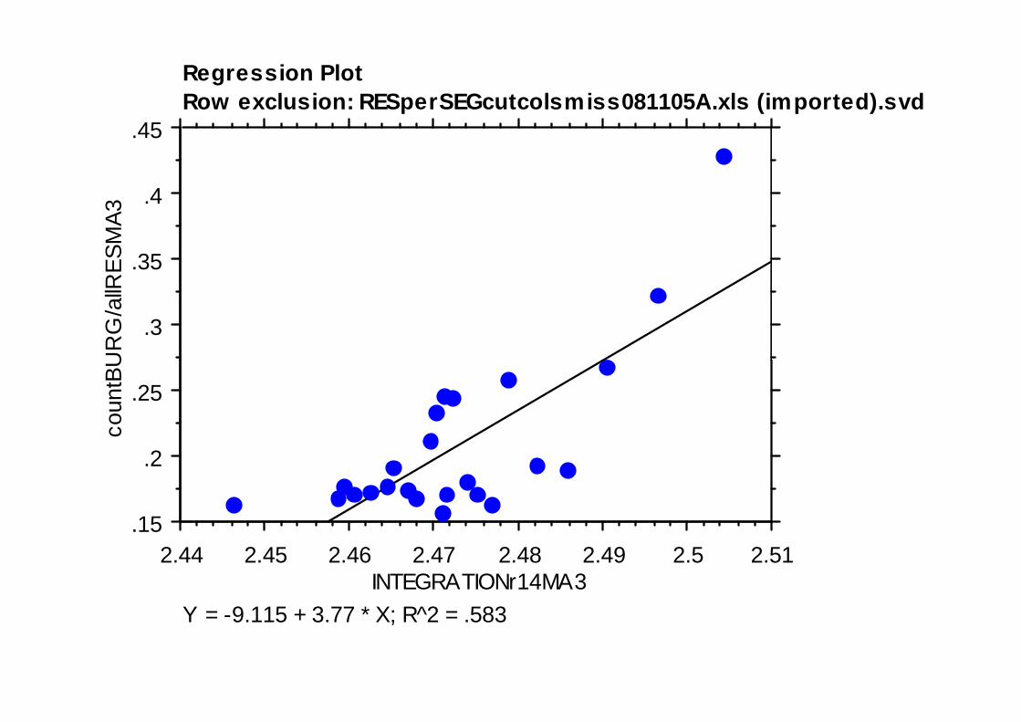
Regression PlotRow exclusion: RESperSEGcutcolsmiss081105A.xls (imported).svd

.15

.2

.25

coun

tBU

RG

/allR

ES

MA

3

2.44 2.45 2.46 2.47 2.48 2.49 2.5 2.51INTEGRATIONr14MA3

Y = -9.115 + 3.77 * X; R^2 = .583

.15

.155

.16

.165

.17

.175

.18co

untB

UR

G/a

llRE

SM

A3

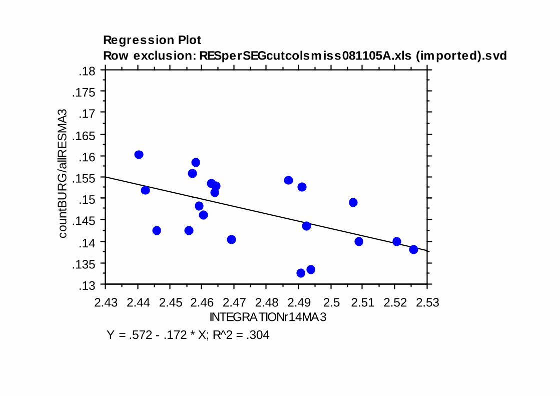
Regression PlotRow exclusion: RESperSEGcutcolsmiss081105A.xls (imported).svd

.13

.135

.14

.145

.15

coun

tBU

RG

/allR

ES

MA

3

2.43 2.44 2.45 2.46 2.47 2.48 2.49 2.5 2.51 2.52 2.53INTEGRATIONr14MA3

Y = .572 - .172 * X; R^2 = .304

.013

.014

.015

.016

.017

totR

OB

/tots

egLE

NG

TH

MA

3

totROB/totsegLENGTHMA3


number of dw ellings per segment

.008

.009

.01

.011

.012

totR

OB

/tots

egLE

NG

TH

MA

3

-2.6

-2.4

-2.2

-2

-1.8

-1.6

log(

RO

B/L

EN

GT

H)/

(RE

S/N

ON

RE

SM

A3)

log(ROB/LENGTH)/(RES/NONRESMA3)


number of dw ellings per segment

-3.6

-3.4

-3.2

-3

-2.8

-2.6

log(

RO

B/L

EN

GT

H)/

(RE

S/N

ON

RE

SM

A3)

1

1.2

1.4

1.6

1.8

2

Var

iabl

es

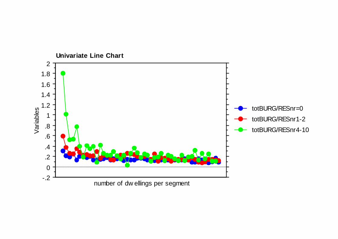
totBURG/RESnr1-2

totBURG/RESnr=0


number of dw ellings per segment-.2

0

.2

.4

.6

.8

Var

iabl

es

totBURG/RESnr4-10

totBURG/RESnr1-2

4.2

4.25

4.3

4.35

4.4

4.45

4.5

SE

GM

EN

Tlin

ks(M

A2)

SEGMENTlinks(MA2)


+1 SD

increasing robberyper unit of street length

3.95

4

4.05

4.1

4.15

4.2

SE

GM

EN

Tlin

ks(M

A2)

SEGMENTlinks(MA2)

Mean

-1 SD

19

20

21

22

23

24

25

avB

UIL

ING

dist

ance

(MA

2)

avBUILINGdistance(MA2)


Mean

+1 SD


14

15

16

17

18

19

avB

UIL

ING

dist

ance

(MA

2)

avBUILINGdistance(MA2)-1 SD

-1.4

-1.2

-1

-.8

-.6

-.4

logN

ON

RE

S/R

ES

MA

2

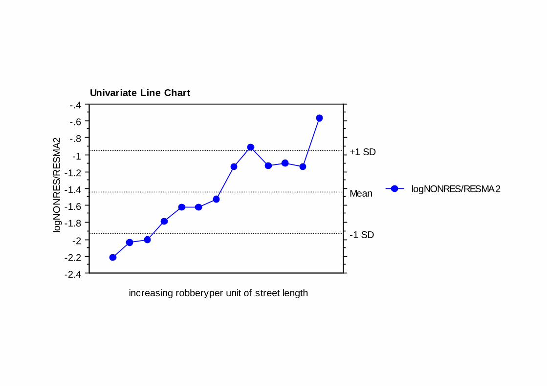
logNONRES/RESMA2


Mean

+1 SD


-2.4

-2.2

-2

-1.8

-1.6

-1.4

logN

ON

RE

S/R

ES

MA

2

logNONRES/RESMA2Mean

-1 SD

6.2

6.4

6.6

6.8

7

7.2

7.4

axC

ON

NM

A2

axCONNMA2


+1 SD


5.2

5.4

5.6

5.8

6

6.2

axC

ON

NM

A2

axCONNMA2

Mean

-1 SD

140

160

180

200

220

SE

Gle

ngth

MA

2

SEGlengthMA2


Mean

+1 SD


60

80

100

120

140

SE

Gle

ngth

MA

2

SEGlengthMA2

-1 SD

800

1000

1200

1400co

untR

OB


0

200

400

600coun

tRO

B

06-09 09-12 12-15 15-18 18-21 21-00 00-03 03-06 time periods

7.42

7.44

7.46

7.48

7.5lo

cal i

nteg

ratio

n


06-09 09-12 12-15 15-18 18-21 21-00 00-03 0306 time periods

7.34

7.36

7.38

7.4

7.42

loca

l int

egra

tion

Are some kinds of dwellings safer than others ?

The safety of dwellings is affected by two simple interacting factors:- the number of sides on which the dwelling is exposed to the public

realm - so flats have least risk and detached houses most- the social class of the inhabitants

All classes tend to be safer in flats, but with increasing wealth the All classes tend to be safer in flats, but with increasing wealth the advantage of living in a flat rather than a house increase, as does the disadvantage of living in a house - in spite of the extra investment that better off people make in security alarms.

Purpose built flats are much safer than converted flats. The overall advantage of flats is in spite of the high vulnerability of converted flats

Is density good or bad ?

Higher local ground level densities of both dwellings and people reducerisk, off the ground density less so, but overall density is beneficial.

Does it matter how we group dwellings ?

• The larger the numbers of dwellings on the street segment (the section of a street between intersections, and so one face of an urban block) the lower the risk of crime.

• This applies to cul de sacs and to through streets, and has a greater effect than either being in a cul de sac or being on a through street. The more immediate neighbours you have the safer you are.immediate neighbours you have the safer you are.

Are cul de sacs safe or unsafe ?

Simple linear cul de sacs with good numbers of dwellings set into a network of through streets tend to be safe, but this does not extend either to small cul de sacs, or complex hierarchies of cul de sacs.

This interacts with social class. Small numbers of well-off dwellings in cul de sacs are more at high risk than a similar group of poor dwellings, while the sacs are more at high risk than a similar group of poor dwellings, while the opposite is the case in grid like layouts where better off dwellings are less at risk than less advantaged dwellings.

Is movement in your street good or bad ?

• Local movement is beneficial, larger scale movement not so - BUT

• For large scale movement, spatially integrated street segments (more movement potential) are advantageous with a high number of dwellings per segment, but disadvantageous with a low number - one of many flipover effects. effects.

Is mixed use beneficial or not ?

There is greater crime risk on mixed use street segments where residence levels are low, but this extra risk is neutralised with increased residential population.

So small numbers of residents in mixed use areas are at risk, but larger number of residents virtually eliminate this.number of residents virtually eliminate this.

Should residential areas be permeable or impermeable ?

• Permeable enough to allow movement in all directions but no more. Poorly used permeability is a crime hazard.

The importance of residential numbers

• All these results point to the link between the strength of residential numbers and low crime. In the past we though this could only be achieved through cul de sacs and ‘defensible space’ which sought security by keeping strangers out.

• Now it is clear that good residential numbers – a residential culture - play a • Now it is clear that good residential numbers – a residential culture - play a key role in security in all parts of the city, in mixed use areas as much as in residential areas.

Documents

Prof Bill Hillier - Royal Institute of Technology/Menu/general/column... · Prof Bill Hillier University of London, UK May 20, 2010 Seminar: Security Matters! ... Logistic Model Coefficients