1

Profit Efficiency and Productivity of Vietnamese Banks: A New  

Index Approach 

 

 

 

 

Daehoon Nahm and Ha Thu Vu* 

 

August 2008 

 

 

 

Abstract 

 

In this paper, we analyse the profit efficiency and productivity of the Vietnamese banking sector. The data envelopment analysis (DEA) method is employed to estimate directional distance as a measure of technical inefficiency for each bank’s operation. Then, we introduce a novel approach to efficiency measurement and define technical efficiency, allocative efficiency, and profit efficiency scores in a ratio form. It contrasts with the available Nerlovian approach that measures inefficiency indicators as normalised loss in potential profit. The new approach avoids the problem of negative profits, which is inherent in the widely used approach of normalising with a profit level, and it also provides measures that are bounded between 0 and 1 in line with the traditional concept of efficiency indices.  We also develop a profit‐oriented Malmquist productivity index that is based on directional distances and decompose it into pure technical‐efficiency index, scale‐efficiency index, and technology‐change index. Our analysis reveals that there is little difference in technical efficiency across different types of banks but there exists a huge gap in allocative efficiency between large state‐owned commercial banks and other banks. The paper also analyses the effects of the regulation on the equity capital to risk‐weighted asset ratio and the effects of the regulation on foreign banks’ deposit taking from Vietnamese nationals.    Keywords: Efficiency, Productivity, Directional Distance, DEA, Banking JEL Codes: C43, G21  __________________________ 

* Department of Economics, Macquarie University, NSW 2109    Corresponding author: Daehoon Nahm, Tel) +612 9850 9615, Fax) +612 9850 6069,     Email) dnahm@efs.mq.edu.au 

2

I.  INTRODUCTION  

Since the introduction of the idea and its generalisation by Luenberger (1992) and Chambers 

et al. (1998) respectively, the directional (technology) distance function has now become a 

standard tool to measure profit efficiency and profit‐oriented productivity; see, for example, 

Färe et al. (2004), Peypoch and Solonandrasana (2008), Glass et al. (2006), Blancard et al. 

(2006), and Park and Weber (2006).  It has also become a useful tool to measure efficiency 

or productivity when the production process produces undesirable by‐products, like 

pollution (Chen et al. [2007], Kumar [2006], Jeon and Sickles [2004], Domazlicky and Weber 

[2004], and Chung et al. [1997]). The directional distance function measures the distance 

from a vector of inputs and outputs within a feasible technology set to the technology 

frontier along a chosen directional vector. In contrast to the radial input or output distance 

function, in which efficiency can only be improved by changing all factors in the same 

direction, the directional distance function allows the factors to change in the opposite 

directions, hence enabling us to measure distances to the frontier by simultaneously 

expanding outputs and contracting inputs. Due to that feature of the function, the 

directional distance of an input‐output vector naturally represents its technical inefficiency 

in achieving maximal profit. 

 

Initially, Nerlove (1965) defines profit inefficiency as the difference between the maximum 

profit and actual profit. However, Nerlove’s definition suffers from a fatal flaw as a measure 

of inefficiency: it is sensitive to proportional price changes. Based on the duality between 

the directional distance function and the profit function, Chambers et al. (1998) not only 

introduce a normalisation that overcomes the flaw but they decompose the normalised 

profit inefficiency into the directional distance, as a measure of technical inefficiency, and 

allocative inefficiency, which is residually determined. They show that the normalisation 

factor that naturally emerges from the profit‐maximisation problem as the Lagrange 

multiplier is the “value of the directional vector”. The difference between maximal profit 

and actual profit that is normalised by the value of the directional vector is referred to as 

the Nerlovian profit inefficiency measure. 

 

3

Although the Nerlovian profit inefficiency measure has a strong theoretical underpinning, it 

is at odds with the traditional index approach that measures efficiency/inefficiency as a 

proportion of full efficiency. In the index approach, for instance, if a production unit’s 

efficiency index is say 0.8 it implies that there is room to improve efficiency by 25% 

(=100x[1‐0.8]/0.8). The Nerlovian indicator measures inefficiency as a multiple of the value 

of the directional vector, but what is the value of the directional vector? When the 

directional vector is defined as the actual input‐output vector, it equals the sum of revenue 

and the cost of inputs. Färe et al. (2004) interpret it as a proxy for ‘size’ of the production 

unit. A complication that still remains, however, is that the indicator treats a change in 

revenue and a change in cost asymmetrically even though the resultant change in profit is 

the same. As an illustration, consider two production units, A and B, whose total costs of 

inputs are initially the same at $100m and initial revenues are also the same at $150m. 

Further, maximal profit they can achieve under the given technology and input and output 

prices is assumed to be $100m. Now, assume that A’s revenue drops to $140m while the 

other figures are unchanged. The Nerlovian inefficiency indicator of A (0.25) relative to that 

of B (0.2) is 1.25. However, an increase in cost for A by the same amount leading to the 

same reduction in profit results in the ratio between the Nerlovian profit inefficiency 

indicators of the two firms being 1.15 (=0.23/0.20). The reason for this asymmetry is that a 

change in revenue affects the numerator and the denominator of the Nerlovian indicator in 

the opposite directions, hence amplifying the effect. 

 

The present paper attempts to bring profit‐efficiency measures into line with the traditional 

index approach by introducing a method to incorporate directional distances into profit 

efficiency and productivity indices, that is, measures as a proportion of full efficiency. It 

develops the new method utilising the Euclidean distances in the input‐output space. In 

particular, it firstly shows that the Euclidean distances are proportional to profit differences 

and constructs index number formulas measuring technical efficiency, allocative efficiency 

and profit efficiency. Unlike the Nerlovian approach, the allocative efficiency index is 

explicitly derived rather than implicitly determined. The paper also introduces a profit‐

oriented productivity index, in a ratio form, that is consistent with the new efficiency indices. 

It contrasts with the available Luenberger productivity indicator which is consistent with the 

4

Nerlovian efficiency measures. The productivity index is then decomposed into pure 

technical efficiency index, scale efficiency index and technology‐change index. 

   

We apply the new method to the analysis of the profit efficiency of the Vietnamese banking 

sector. Importance of an efficiently operating banking sector to the health of the whole 

economy could never be over‐emphasised for any country, but the Vietnamese banking 

sector is especially of interest since it has been undergoing a rapid reform process for the 

last two decades following the introduction of the reform package known as Doi Moi 

(renovation). It has been changing from virtual nonexistence where all financial matters 

were tightly controlled and operated by a single central bank (State Bank of Vietnam, SBV) 

to a two‐tier system where commercial banking functions were transferred to a few state‐

owned commercial banks in the late 1980s, and then to a more liberalised and privatised 

banking sector since the early 1990s where tens of joint‐stock commercial banks, that are 

jointly owned by the state and private owners, and foreign bank branches are operating. 

The Asian financial crisis has provoked the introduction of further measures in the late 

1990s and early 2000s, speeding up the reform process. So, it is about the right time to 

examine the effectiveness of the reform policies on the efficiency and productivity of banks 

and to review the policies with a view to possible adjustments. Given its importance, it is 

surprising to find that there exists only one study on the efficiency of the Vietnamese 

banking sector. Nguyen (2007) uses an input‐oriented DEA model to analyse the cost 

efficiency of 13 banks over three‐year period between 2001 and 2003. He finds that the 

main source of cost inefficiency (0.394 on average) is allocative inefficiency (0.385 on 

average) rather than technical inefficiency (0.082 on average). The present paper is different 

from Nguyen (2007) in two important aspects: one is that it analyses a more comprehensive 

data set covering a group of 56 banks over the seven‐year period 2000‐2006, and the other 

is that it uses a more advanced methodology to analyse profit efficiency using the 

directional distance function. 

 

The paper is organised as follows. Next section introduces the new efficiency and 

productivity indices. It also explicitly specifies the DEA problems involved. Section III 

5

describes the data while Section IV reports the empirical results. The final section provides 

conclusions.    

 

II.  EFFICIENCY AND PRODUCTIVITY INDICES 

 

 

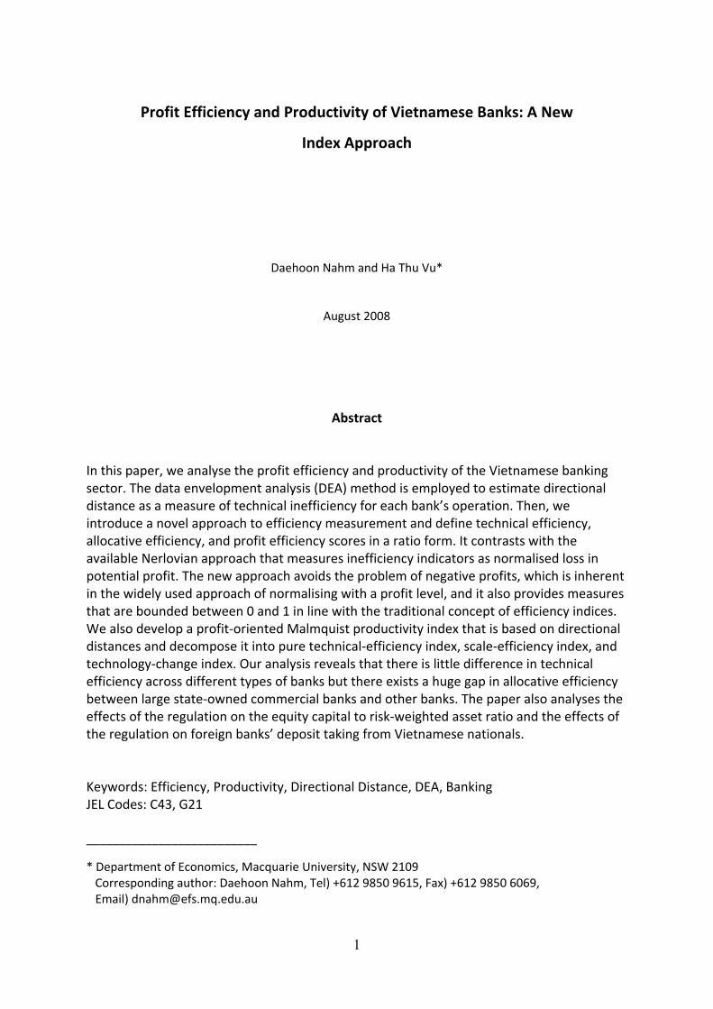
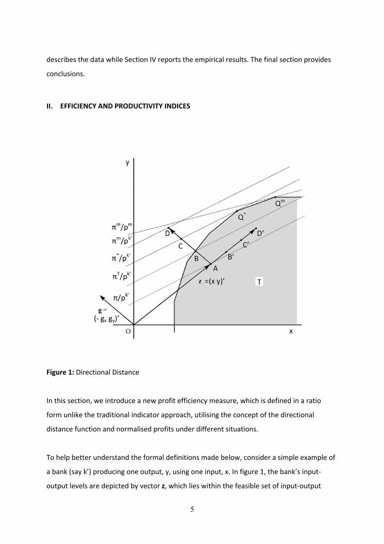
Figure 1: Directional Distance 

 

In this section, we introduce a new profit efficiency measure, which is defined in a ratio 

form unlike the traditional indicator approach, utilising the concept of the directional 

distance function and normalised profits under different situations.  

 

To help better understand the formal definitions made below, consider a simple example of 

a bank (say k’) producing one output, y, using one input, x. In figure 1, the bank’s input‐

output levels are depicted by vector z, which lies within the feasible set of input‐output 

6

combinations under the available technology (shaded area). The figure shows that the 

bank’s current operation is technically inefficient as z is off the frontier that defines the 

feasible technology set. If we decide to measure how much the bank can increase its profit 

by simultaneously reducing input and increasing output along the directional vector given 

by g = (‐gx gy)’, the changes that are required for the bank to be technically efficient will be 

represented in the figure by the movement from the current point, A, to point B where 

vector AD that is parallel to g passes through the frontier. So, a natural measure of technical 

inefficiency would be a ratio of the distance between A and B, |AB|, to the total distance 

from O to A and then B, namely |OA|+|AB|. When point B’ is located along the extension of 

z so that |AB|=|AB’|, the technical inefficiency score can be defined as |AB’|/|OB’|, and 

hence the technical efficiency score as |OA|/|OB’|. 

 

The parallel lines passing through points A, B, C and D on vector AD are the price line the 

bank is facing, whose slope equals the input price, denoted wk’, divided by the output price, 

denoted pk’. When the bank is allowed to change the input‐output mix in any direction, the 

maximum profit can then be achieved at a point where the price line is tangent to the 

feasible set, namely at point Q*. Let C be the point where the price line that is tangent to 

the frontier crosses vector AD, and let π, πT, and π* denote the actual profit at point A, the 

profit at the technically efficient point B and the optimal profit achievable under the given 

price vector (wk’ pk’)’ at point Q* respectively. Then, the ratio between the differences in the 

profits given by (πT−π)/(π*−π), equals |AB|/|AC| since the heights of the parallel price lines 

along the vertical axis represent profit levels normalised by the same constant which is 

output price, pk’. It implies that what |AB| is to (πT−π) is what |AC| is to (π*−π). That is, 

when |AB| is proportional to the additional profit that the bank can achieve when it 

becomes technically efficient, |AC| is proportional by the same proportion to the additional 

profit the bank can achieve when it is allowed to change the input‐output mix and achieve 

the maximum profit under the given prices. Furthermore, as (π*−π) equals (πT−π)+(π*−πT) 

and |AC| equals |AB|+|BC|, |BC| is proportional by the same proportion to (π*−πT), which 

is the additional profit the bank can achieve over the profit it makes at the technically 

efficient point along the given directional vector, when it changes input‐output bundle and 

becomes allocatively efficient on top of being technically efficient. So, analogous to the 

7

definition of technical inefficiency, allocative inefficiency can be defined as 

|BC|/(|OA|+|AB|+|BC|), which is equal to |B’C’|/|OC’| when C’ is located along vector OD’ 

so that |AC|=|AC’|. The allocative efficiency index is then defined by |OB’|/|OC’|, and the 

profit efficiency index by |OA|/|OC’|.  

 

As should be the case, the profit efficiency is the product of technical efficiency and 

allocative efficiency. Note that profits may be negative but π* will be always at least as high 

as πT which is in turn at least as high as π and hence negative profits will not cause a trouble 

in the definitions of indices. When π equals π*, technical efficiency, allocative efficiency and 

profit efficiency will be all one. 

 

For the formal definitions of the efficiency scores, consider banking industry where banks 

produce M outputs using N inputs, that is, input vector x ∈   NR +  and output vector y ∈    MR + .  

Let z = (x’ y’)’ ∈   MNR ++  be the actual input output vector, g = (−gx’ gy’)’ ∈   MNR +

+  be the 

directional vector, and p = (−w’ p’)’ ∈   NR −−  × MR ++  be the vector of negative input prices and 

positive output prices.  

 

We define the feasible set T � NR + ×MR +  under the available technology as 

 

    T = {(x,y): x can produce y}.              (1) 

 

Then, the directional (technology) distance function is defined by (Luenberger[1992] and 

Chambers et al.[1998]): 

 

β* = D (z;g,T) = maxβ{β: (z + βg) ∈ T} (2)

where β* is the solution to the conditional maximisation problem. Since z ∈  T, β* is non‐

negative.1 If β* equals zero, it implies that it is technically impossible to simultaneously 

contract inputs and expand outputs from the current levels and hence z is technically 

                                                            1  See Lemma 2.1 of Chambers et al. (1998, p354). 

8

efficient. When β* is greater than zero, on the other hand, it is implied that there is room for 

an increase in the profit by producing more outputs using less inputs. The maximum 

simultaneous reductions in the inputs and increases in the outputs that the bank can make 

along the directional vector are by β*g, whose equivalence in Figure 1 is AB. In that case, the 

maximum profit achievable is given by  

 

    πT = p∙(z + β*g) = p∙z + β*p∙g = π + β*δ           (3) 

 

where π is the actual profit and δ = p∙g = w’gx + p’gy which is strictly positive given that g is 

not a null vector. Rearranging the equation for β* yields 

 

    β* = (πT − π)/δ.                 (4) 

 

Now, write the maximum profit the bank can achieve when changes in input‐output bundle 

are allowed for in a similar way: 

 

    π* = p∙(z + λ1g) = p∙z + λ1p∙g = π + λ1δ          (5) 

 

where λ1 is non‐negative scalar value that makes the first equation in (5) hold. The new 

input‐output vector, (z + λ1g), may not be feasible under T, but a λ1 should exist to make the 

equation algebraically true and that is all needed here.  Rearranging for λ1 gives  

 

    λ1 = (π* − π)/δ.                 (6) 

 

In Figure 1, |AB| which represents technical inefficiency equals β* times the length of the 

directional vector, i.e. β*|g|. This implies that |AC| equals λ1 times the length of the 

directional vector, i.e. λ1|g|, because |AB|/|AC| equals (πT−π)/(π*−π) = β*/λ1. So, |BC| 

which represents allocative inefficiency equals λ1|g|− β*|g|. Comparing equations (3) and 

(5) reveals that λ1 ≥ β* because π* ≥ πT and δ > 0. Thus, λ1|g|− β

*|g| ≥ 0.      

 

9

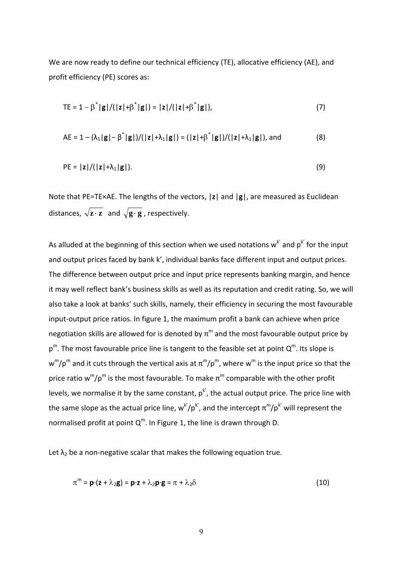
We are now ready to define our technical efficiency (TE), allocative efficiency (AE), and 

profit efficiency (PE) scores as: 

 

  TE = 1 − β*|g|/(|z|+β*|g|) = |z|/(|z|+β*|g|),          (7) 

 

  AE = 1 – (λ1|g|− β*|g|)/(|z|+λ1|g|) = (|z|+β*|g|)/(|z|+λ1|g|), and    (8) 

 

  PE = |z|/(|z|+λ1|g|).                (9) 

 

Note that PE=TE×AE. The lengths of the vectors, |z| and |g|, are measured as Euclidean 

distances,  zz ⋅   and  gg ⋅ , respectively. 

 

As alluded at the beginning of this section when we used notations wk’ and pk’ for the input 

and output prices faced by bank k’, individual banks face different input and output prices. 

The difference between output price and input price represents banking margin, and hence 

it may well reflect bank’s business skills as well as its reputation and credit rating. So, we will 

also take a look at banks’ such skills, namely, their efficiency in securing the most favourable 

input‐output price ratios. In figure 1, the maximum profit a bank can achieve when price 

negotiation skills are allowed for is denoted by πm and the most favourable output price by 

pm. The most favourable price line is tangent to the feasible set at point Qm. Its slope is 

wm/pm and it cuts through the vertical axis at πm/pm, where wm is the input price so that the 

price ratio wm/pm is the most favourable. To make πm comparable with the other profit 

levels, we normalise it by the same constant, pk’, the actual output price. The price line with 

the same slope as the actual price line, wk’/pk’, and the intercept πm/pk’ will represent the 

normalised profit at point Qm. In Figure 1, the line is drawn through D. 

 

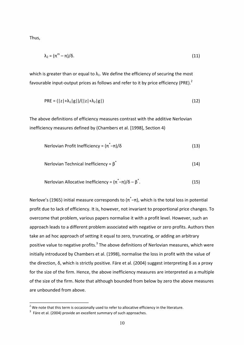
Let λ2 be a non‐negative scalar that makes the following equation true. 

 

    πm = p∙(z + λ2g) = p∙z + λ2p∙g = π + λ2δ          (10) 

 

10

Thus, 

 

    λ2 = (πm – π)/δ.                (11) 

     

which is greater than or equal to λ1. We define the efficiency of securing the most 

favourable input‐output prices as follows and refer to it by price efficiency (PRE).2 

 

    PRE = (|z|+λ1|g|)/(|z|+λ2|g|)            (12) 

 

The above definitions of efficiency measures contrast with the additive Nerlovian 

inefficiency measures defined by (Chambers et al. [1998], Section 4) 

 

    Nerlovian Profit Inefficiency = (π*−π)/δ            (13) 

 

    Nerlovian Technical Inefficiency = β*            (14) 

 

    Nerlovian Allocative Inefficiency = (π*−π)/δ – β*.        (15) 

 

Nerlove’s (1965) initial measure corresponds to (π*−π), which is the total loss in potential 

profit due to lack of efficiency. It is, however, not invariant to proportional price changes. To 

overcome that problem, various papers normalise it with a profit level. However, such an 

approach leads to a different problem associated with negative or zero profits. Authors then 

take an ad hoc approach of setting it equal to zero, truncating, or adding an arbitrary 

positive value to negative profits.3 The above definitions of Nerlovian measures, which were 

initially introduced by Chambers et al. (1998), normalise the loss in profit with the value of 

the direction, δ, which is strictly positive. Färe et al. (2004) suggest interpreting δ as a proxy 

for the size of the firm. Hence, the above inefficiency measures are interpreted as a multiple 

of the size of the firm. Note that although bounded from below by zero the above measures 

are unbounded from above. 

                                                            2 We note that this term is occasionally used to refer to allocative efficiency in the literature.  3  Färe et al. (2004) provide an excellent summary of such approaches. 

11

 

Unlike the Nerlovian measures, the measures introduced in the present paper are defined 

as a ratio between distances and they are bounded between 0 and 1, hence making the 

interpretation more in line with the traditional concept of efficiency indices. Furthermore, 

while the Nerlovian allocative inefficiency measure is defined as a residual, our allocative 

efficiency measure is explicitly defined; see (8). 

 

We also analyse the change in productivity over each pair of consecutive years using a 

modified version of the Malmquist productivity index. Our Malmquist productivity index 

builds on the Malmquist productivity index of Caves et al. (1982), which is based on radial 

input or output distances, and it measures profit‐oriented productivity based on directional 

distances. As we intend to decompose a change in productivity into pure technical efficiency 

change, scale efficiency change, and technology change, we measure distances of an input‐

output vector against both the constant returns to scale (CRS) and the variable returns to 

scale (VRS) frontiers. Then, the difference between the distance to the CRS frontier and the 

distance to the VRS frontier will represent scale inefficiency.  

 

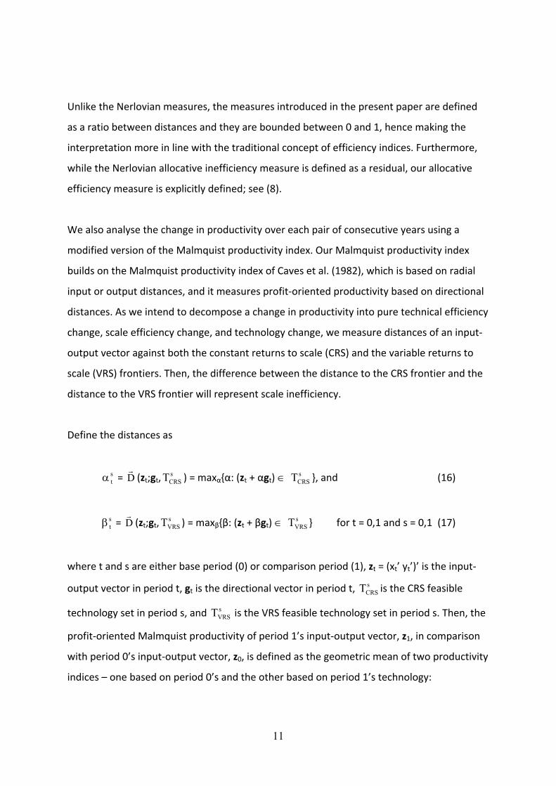
Define the distances as 

 

    stα  = D (zt;gt,

sCRST ) = maxα{α: (zt + αgt) ∈   s

CRST }, and      (16) 

 

    stβ  = D (zt;gt,

sVRST ) = maxβ{β: (zt + βgt) ∈   s

VRST }  for t = 0,1 and s = 0,1  (17) 

 

where t and s are either base period (0) or comparison period (1), zt = (xt’ yt’)’ is the input‐

output vector in period t, gt is the directional vector in period t,  sCRST is the CRS feasible 

technology set in period s, and  sVRST  is the VRS feasible technology set in period s. Then, the 

profit‐oriented Malmquist productivity of period 1’s input‐output vector, z1, in comparison 

with period 0’s input‐output vector, z0, is defined as the geometric mean of two productivity 

indices – one based on period 0’s and the other based on period 1’s technology: 

 

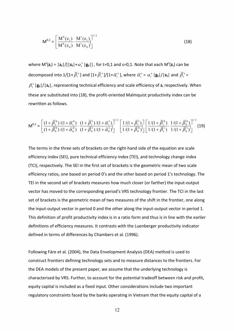
12

    M0,1 = 2/1

01

11

00

10

)z(M)z(M

)z(M)z(M

⎥⎦

⎤⎢⎣

⎡⋅               (18) 

 

where Ms(zt) = |zt|/[|zt|+stα |gt|] , for t=0,1 and s=0,1. Note that each M

s(zt) can be 

decomposed into 1/[1+ stβ ] and [1+ s

tβ ]/[1+ stα ], where  s

tα =  stα |gt|/|zt| and 

stβ = 

stβ |gt|/|zt|, representing technical efficiency and scale efficiency of zt respectively. When 

these are substituted into (18), the profit‐oriented Malmquist productivity index can be 

rewritten as follows. 

 

M0,1 = 2/1

10

10

11

11

00

00

01

01

)1/()1()1/()1(

)1/()1()1/()1(

⎥⎦

⎤⎢⎣

⎡++++

⋅++++

αβαβ

αβαβ

⎥⎦

⎤⎢⎣

⎡++

)1/(1)1/(1

00

11

ββ

2/1

10

00

11

01

)1/(1)1/(1

)1/(1)1/(1

⎥⎦

⎤⎢⎣

⎡++

⋅++

ββ

ββ

(19) 

 

The terms in the three sets of brackets on the right‐hand side of the equation are scale 

efficiency index (SEI), pure technical efficiency index (TEI), and technology change index 

(TCI), respectively. The SEI in the first set of brackets is the geometric mean of two scale 

efficiency ratios, one based on period 0’s and the other based on period 1’s technology. The 

TEI in the second set of brackets measures how much closer (or farther) the input‐output 

vector has moved to the corresponding period’s VRS technology frontier. The TCI in the last 

set of brackets is the geometric mean of two measures of the shift in the frontier, one along 

the input‐output vector in period 0 and the other along the input‐output vector in period 1. 

This definition of profit productivity index is in a ratio form and thus is in line with the earlier 

definitions of efficiency measures. It contrasts with the Luenberger productivity indicator 

defined in terms of differences by Chambers et al. (1996). 

 

Following Färe et al. (2004), the Data Envelopment Analysis (DEA) method is used to 

construct frontiers defining technology sets and to measure distances to the frontiers. For 

the DEA models of the present paper, we assume that the underlying technology is 

characterised by VRS. Further, to account for the potential tradeoff between risk and profit, 

equity capital is included as a fixed input. Other considerations include two important 

regulatory constraints faced by the banks operating in Vietnam that the equity capital of a 

13

domestic bank should be at least a certain proportion of its total risk‐weighted asset 

(capital‐adequacy constraint) and that the total amount of deposits by Vietnamese nationals 

with a foreign bank cannot exceed a set multiple of its equity capital (deposit constraint). 

We will estimate the models with and without the capital‐adequacy and deposit constraints 

to analyse the effects of those constraints.   

 

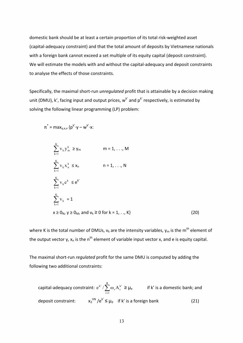
Specifically, the maximal short‐run unregulated profit that is attainable by a decision making 

unit (DMU), k’, facing input and output prices, wk’ and pk’ respectively, is estimated by 

solving the following linear programming (LP) problem: 

 

    π* = maxy,x,v {pk’∙y – wk’∙x:  

 

            ∑=

K

1k

kmk yv  ≥ ym    m = 1, . . ., M 

            ∑=

K

1k

knk xv  ≤ xn    n = 1, . . ., N 

            ∑=

K

1k

kkev  ≤ ek’   

            ∑=

K

1kkv  = 1   

            x ≥ 0N, y ≥ 0M, and vk ≥ 0 for k = 1, . ., K}          (20) 

 

where K is the total number of DMUs, vk are the intensity variables, ym is the mth element of 

the output vector y, xn is the nth element of variable input vector x, and e is equity capital.  

 

The maximal short‐run regulated profit for the same DMU is computed by adding the 

following two additional constraints: 

 

  capital‐adequacy constraint:  ∑=

ωR

1r

'krr

'k A/e  ≥ μe  if k’ is a domestic bank; and 

  deposit constraint:  x3VN /ek’ ≤ μd  if k’ is a foreign bank      (21) 

               

14

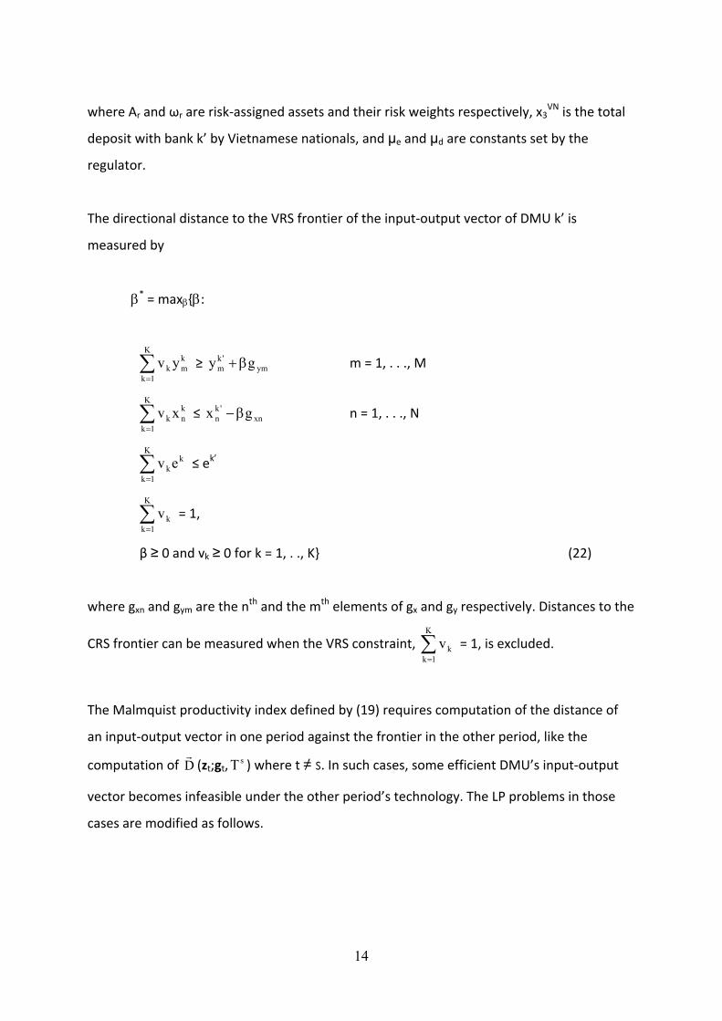
where Ar and ωr are risk‐assigned assets and their risk weights respectively, x3VN is the total 

deposit with bank k’ by Vietnamese nationals, and μe and μd are constants set by the 

regulator. 

 

The directional distance to the VRS frontier of the input‐output vector of DMU k’ is 

measured by 

 

    β* = maxβ{β: 

 

      ∑=

K

1k

kmk yv  ≥  ym

'km gy β+     m = 1, . . ., M 

      ∑=

K

1k

knk xv  ≤  xn

'kn gx β−     n = 1, . . ., N 

      ∑=

K

1k

kkev  ≤ ek’  

      ∑=

K

1kkv  = 1,    

          β ≥ 0 and vk ≥ 0 for k = 1, . ., K}            (22) 

     

where gxn and gym are the nth and the mth elements of gx and gy respectively. Distances to the 

CRS frontier can be measured when the VRS constraint, ∑=

K

1kkv  = 1, is excluded. 

 

The Malmquist productivity index defined by (19) requires computation of the distance of 

an input‐output vector in one period against the frontier in the other period, like the 

computation of D (zt;gt, sT ) where t ≠ s. In such cases, some efficient DMU’s input‐output 

vector becomes infeasible under the other period’s technology. The LP problems in those 

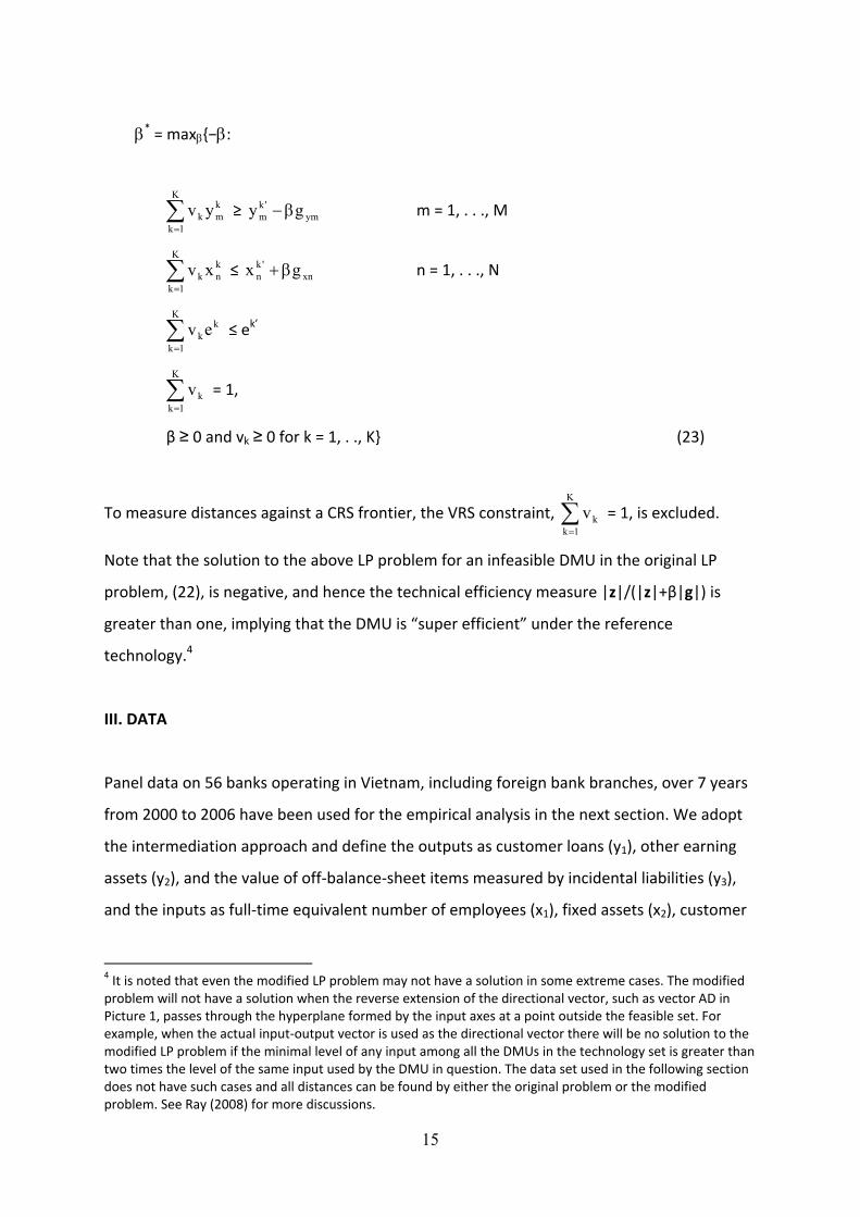
cases are modified as follows. 

 

15

  β* = maxβ{−β: 

 

      ∑=

K

1k

kmk yv  ≥  ym

'km gy β−     m = 1, . . ., M 

      ∑=

K

1k

knk xv  ≤  xn

'kn gx β+     n = 1, . . ., N 

      ∑=

K

1k

kkev  ≤ ek’  

      ∑=

K

1kkv  = 1,    

          β ≥ 0 and vk ≥ 0 for k = 1, . ., K}            (23) 

 

To measure distances against a CRS frontier, the VRS constraint, ∑=

K

1kkv  = 1, is excluded. 

Note that the solution to the above LP problem for an infeasible DMU in the original LP 

problem, (22), is negative, and hence the technical efficiency measure |z|/(|z|+β|g|) is 

greater than one, implying that the DMU is “super efficient” under the reference 

technology.4  

 

III. DATA 

 

Panel data on 56 banks operating in Vietnam, including foreign bank branches, over 7 years 

from 2000 to 2006 have been used for the empirical analysis in the next section. We adopt 

the intermediation approach and define the outputs as customer loans (y1), other earning 

assets (y2), and the value of off‐balance‐sheet items measured by incidental liabilities (y3), 

and the inputs as full‐time equivalent number of employees (x1), fixed assets (x2), customer 

                                                            4 It is noted that even the modified LP problem may not have a solution in some extreme cases. The modified problem will not have a solution when the reverse extension of the directional vector, such as vector AD in Picture 1, passes through the hyperplane formed by the input axes at a point outside the feasible set. For example, when the actual input‐output vector is used as the directional vector there will be no solution to the modified LP problem if the minimal level of any input among all the DMUs in the technology set is greater than two times the level of the same input used by the DMU in question. The data set used in the following section does not have such cases and all distances can be found by either the original problem or the modified problem. See Ray (2008) for more discussions. 

16

deposits and other borrowed funds (x3) plus equity capital (e) as a fixed input. All input and 

output values are deflated with the consumer price index. 

 

The price of y1, denoted p1, is derived as the amount of interest income from customer 

loans divided by the amount of customer loans. The price of y2, denoted p2, is derived 

similarly as the amount of other interest and investment income divided by the amount of 

other earning assets. Necessary information to derive the price for off‐balance‐sheet items 

(y3), denoted p3, is not available for all banks. Hence, we compute p3 as non‐interest non‐

investment income divided by the value of off‐balance‐sheet items for the banks where 

separate series are available. Then, the average of those p3 values in each year is used as the 

price of y3 for all banks in that year assuming that p3 is identical for all banks in each year.  

The price of x1, denoted w1, is derived similarly to p3 since the data for full‐time equivalent 

number of employees are not available for all banks. That is, w1 is derived by dividing 

personnel expenses by full‐time equivalent number of employees for those banks where the 

information is available, and then the average of those w1’s within each year is used as the 

price of x1 for all banks in that year. Then, the numbers of employees for the banks where 

the information is not available are derived by dividing personnel expenses by w1. Although 

this is not as good as direct observation, it may not be too unrealistic to assume that all 

banks face the same level of labour cost in each year. The price of x2, denoted w2, is derived 

as other non‐interest expenses divided by the total value of fixed assets, while the price of 

x3, denoted w3, is derived as interest expenses paid for deposits and other borrowed funds 

divided by the total amount of customer deposits and other borrowed funds. 

 

17

Table 1: Data Summary – Average per Bank over Whole Sample Period    All Banks  SOBsa  Urban  Rural  JVBsb  Foreign Number of Banks  56  5  20  10  4  17 Outputs y1: Customer Loansd 

 y2: Other Earning 

Assetsd 

y3: OBS Itemsd 

 

 5,382.2 

(16,701.6)c 

2,217.4 (6,561.9) 

767.1 (1,983.9) 

46,739.8(35,305.1)16,185.6

(15,960.3)5,087.2

(4,615.9) 

1,935.5(2,101.5)1,056.2

(1,804.5)502.9

(726.6) 

140.7(146.5)

68.2(211.6)

18.5(66.2) 

 924.6 

(787.8) 787.1 

(468.8) 233.8 

(142.8) 

1,405.1(1,179.9)1,075.9

(1,164.6)373.2

(314.2) Variable Inputs x1: Employeese 

 x2: Fixed Assets

d 

 x3: Deposits & 

Borrowed Fundsd 

 1,341.1 

(4,426.9) 119.7 

(351.1) 8,044.3 

(22,715.6) 

11,065.9(10,797.1)

980.8(738.4)

67,804.1(42,473.9) 

506.6(549.3)

68.0(79.9)

3,220.8(3,978.6) 

47.0(37.8)

5.9(10.4)171.3

(242.5) 

 387.3 

(153.1) 21.5 

(11.6) 1,539.7 (754.1) 

448.4(310.5)

17.3(12.6)

2,304.2(2,064.6) 

Output Prices p1: Price of y1

f 

 p2: Price of y2

f 

 p3: Price of y3

f 

 

 0.09 

(0.03) 0.07 

(0.08) 0.09 

(0.02) 

0.11(0.05)0.12

(0.09)0.09

(0.02) 

0.10(0.02)0.08

(0.09)0.09

(0.02) 

0.12(0.03)0.05

(0.05)0.09

(0.02) 

 0.07 

(0.02) 0.08 

(0.04) 0.09 

(0.02) 

0.07(0.03)0.05

(0.06)0.09

(0.02) Variable Input Prices w1: Price of x1

g 

 w2: Price of x2

f 

 w3: Price of x3

f 

 

 33.73 (6.05) 1.37 

(2.81) 0.05 

(0.03) 

33.73(6.13)0.59

(0.28)0.08

(0.03) 

33.73(6.06)0.66

(0.91)0.06

(0.02) 

33.73(6.09)0.65

(0.68)0.07

(0.02) 

 33.73 (6.15) 0.99 

(0.43) 0.04 

(0.02) 

33.73(6.07)2.95

(4.61)0.03

(0.01) Other Variables Equity Capital (fixed 

input)d 

Profitd 

 Profit/Equity Ratio  Risk‐weighted 

Assetsd 

Deposits by Vietnamesed 

 560.9 

(1,196.0) 154.1 

(557.0) 0.18 

(0.17) 5,040.8 

(14,542.4) n.a. 

 

3,695.0(2,190.7)1,285.7

(1,442.0)0.29

(0.20)42,709.8

(28,185.5)n.a.

 

291.6(303.1)

70.8(85.8)0.22

(0.20)2,036.6

(2,450.8)n.a.

 

63.0(137.5)

4.9(8.0)0.17

(0.15)118.9

(163.1)n.a. 

 308.3 (64.3) 35.1 

(22.5) 0.11 

(0.05) 921.6 

(491.6) n.a. 

308.2(102.0)

35.0(32.5)0.11

(0.09)1,360.6

(1,034.4)95.2 

(107.2) a. State‐owned banks b. Banks established as a joint‐venture with foreign entities c. Figures in parentheses are standard deviations. d. Billion Vietnamese Dong (Average DVN/US$ exchange rate during the sample period was around 15,000 DVNs per US$.) e. Full‐time equivalent employees f. Vietnamese Dong g. Million Vietnamese Dong   

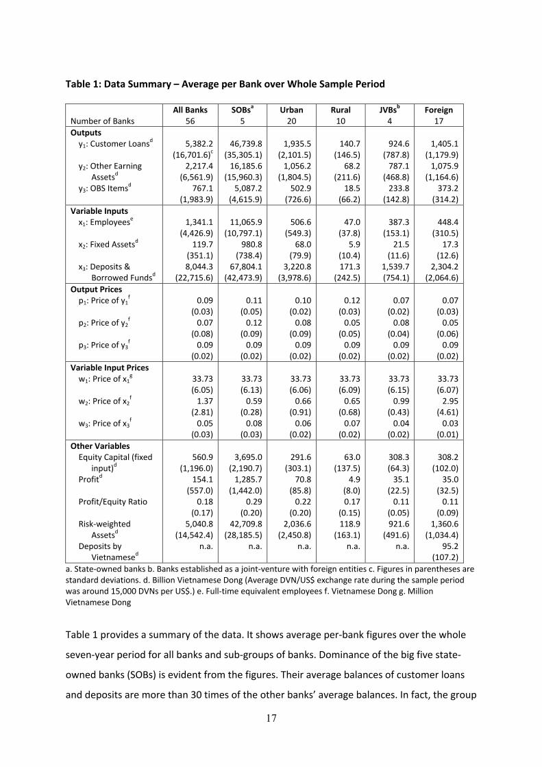
Table 1 provides a summary of the data. It shows average per‐bank figures over the whole 

seven‐year period for all banks and sub‐groups of banks. Dominance of the big five state‐

owned banks (SOBs) is evident from the figures. Their average balances of customer loans 

and deposits are more than 30 times of the other banks’ average balances. In fact, the group 

18

of big five SOBs hold 77% of all customer loans and 75% of all customer deposits and 

borrowed funds. Their average equity capital size is only 15 times the average equity capital 

of all the other banks, but their average profit is almost 30 times the average profit of the 

other banks, leading to their average profit‐equity capital ratio of 29% being significantly 

higher than the others’ 11% to 22%. Urban banks are much larger than rural banks but only 

marginally larger than joint‐venture banks or foreign banks. There appears to be little 

difference between joint‐venture banks and foreign banks in terms of business and profit 

sizes. The huge differences in the input and output variables across subgroups, especially 

between SOBs and rural banks, are reflected in the standard errors for the group of all banks 

that are roughly three times their corresponding means. 

 

The capital‐adequacy regulation is applied only to the domestic and joint‐venture banks and 

not applied to the 17 foreign banks, while the deposit regulation is applied only to the 

foreign banks. The capital‐adequacy regulation currently adopted by the Vietnamese 

regulator is the minimum ratio of equity capital to risk weighted assets. A bank is regarded 

as adequately capitalised if the ratio is at least 8%, which is equivalent to μe in (21). Total 

risk‐weighted assets in (21) is computed as  

 

    Risk‐weighted assets = ω1y1 + ω2y2 + ω3y3c + ω4x2 + ω5OA      (24) 

 

where ωi are risk weights, c is the conversion ratio for off‐balance‐sheet items, and OA is 

other assets which is explained below. Risk weights for the variables defined in the present 

paper are estimated as a weighted average of the risk weights for the sub‐assets included in 

each variable. The risk weight for Customer Loans (y1) is 55% reflecting various degrees of 

risk associated with loans with different types of securities, ranging from 0% for loans 

secured by deposits with the bank itself to 100% for loans secured by a third‐party property. 

Other Earning Assets (y2) carries a risk weight of 25% representing balances with other 

financial institutions and securities. Off‐balance‐sheet Items (y3) is converted to a value 

equivalent to balance‐sheet items by multiplying by the conversion ratio of 0.5 before the 

risk weight 50% is applied. Fixed Assets (x2) carries a risk weight of 100%. There are other 

assets (OA) that are not included in any of the output variables or Fixed Assets, while they 

19

should be included in the measure of risk‐weighted assets for capital‐adequacy. Those 

assets include balance with the central bank, cash and equivalent, and non‐performing loans. 

OA carries a risk weight of 60%.   

 

Note that the capital‐adequacy constraint is imposed in the profit‐maximisation problem, 

(20), as 

 

    ω1y1 + ω2y2 + ω3y3c + ω4x2 ≤ (ek’/μe) – ω5OA

k’        (25) 

     

while it is imposed for the directional distance function, (22), as 

 

    β(ω1gy1 + ω2gy2 + ω3gy3c − ω4gx2) ≤  

      (ek’/μe) – (ω1y1k’ + ω2y2

k’ + ω3y3k’c + ω4x2

k’ + ω5OAk’).     (26) 

 

Also note that when the bank in question, k’, violates the capital‐adequacy regulation the LP 

problem for the directional distance usually does not have a feasible set, but the LP problem 

for maximum profit may have one. The former is the case because the right‐hand side of 

(26) becomes negative while the term in parentheses on the left‐hand side is usually 

positive. On the other hand, the violation does not automatically make the profit‐

maximisation problem infeasible because an optimum input‐output vector can still be found 

such that the constraint (25) is satisfied. 

 

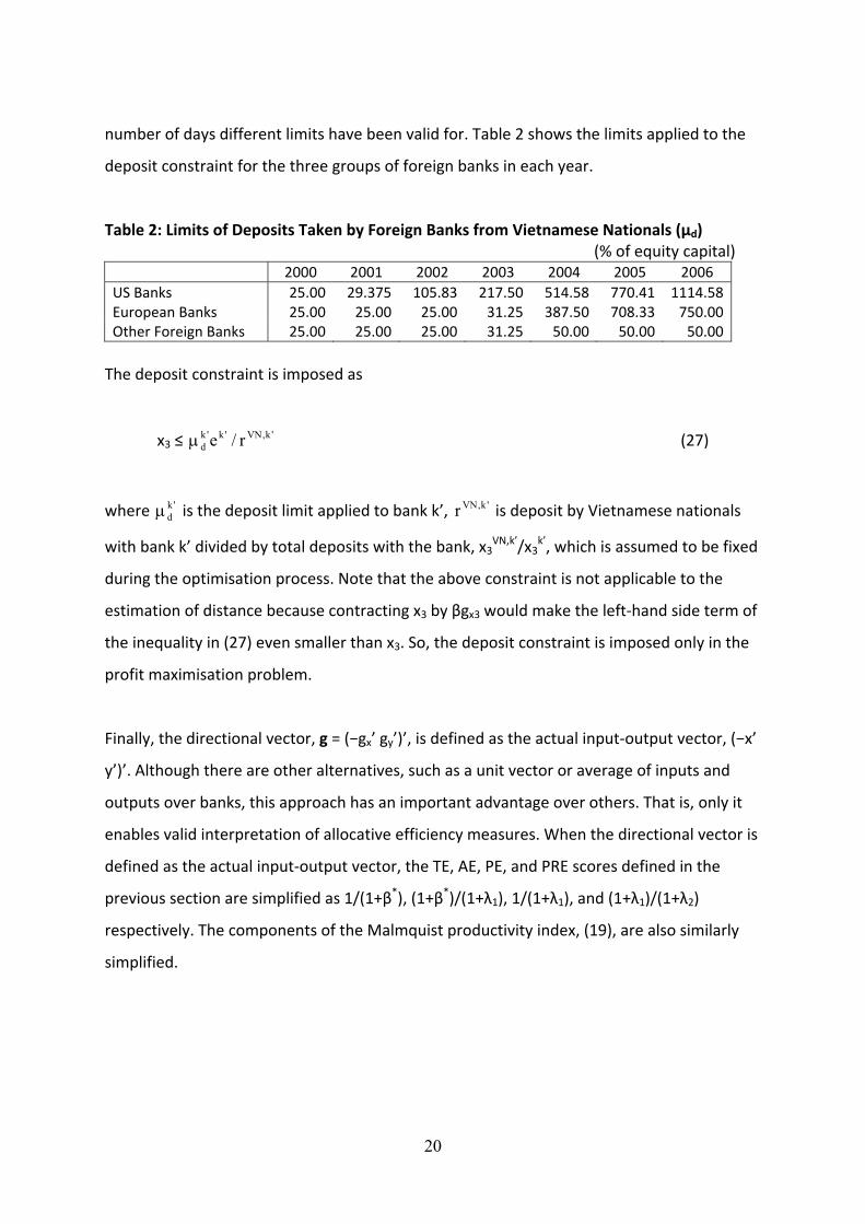
Up to December 2001, the maximum amount of deposits any foreign bank can take from 

Vietnamese nationals (natural or legal persons) had been 25% of equity capital. However, 

the bilateral trade agreements with U.S. and European countries have led to a gradual 

relaxation of this limit to 700% from legal persons plus 650% from natural persons for U.S. 

banks and 400% from legal persons plus 350% from natural persons for European banks by 

the end of 2006. Other foreign banks’ limit has also been relaxed to 50% from October 2003. 

For each year, the limits applied to different groups of foreign banks are computed as a 

weighted average of limits for legal and natural persons with the weights reflecting the 

20

number of days different limits have been valid for. Table 2 shows the limits applied to the 

deposit constraint for the three groups of foreign banks in each year. 

 

Table 2: Limits of Deposits Taken by Foreign Banks from Vietnamese Nationals (μd)                                                                                                                             (% of equity capital)   2000  2001  2002  2003  2004  2005  2006 US Banks  25.00  29.375 105.83 217.50 514.58 770.41  1114.58European Banks  25.00  25.00 25.00 31.25 387.50 708.33  750.00Other Foreign Banks  25.00  25.00 25.00 31.25 50.00 50.00  50.00 The deposit constraint is imposed as 

 

    x3 ≤ 'k,VN'k'k

d r/eμ                 (27) 

 

where  'kdμ  is the deposit limit applied to bank k’,  'k,VNr  is deposit by Vietnamese nationals  

with bank k’ divided by total deposits with the bank, x3VN,k’/x3

k’, which is assumed to be fixed 

during the optimisation process. Note that the above constraint is not applicable to the 

estimation of distance because contracting x3 by βgx3 would make the left‐hand side term of 

the inequality in (27) even smaller than x3. So, the deposit constraint is imposed only in the 

profit maximisation problem. 

 

Finally, the directional vector, g = (−gx’ gy’)’, is defined as the actual input‐output vector, (−x’ 

y’)’. Although there are other alternatives, such as a unit vector or average of inputs and 

outputs over banks, this approach has an important advantage over others. That is, only it 

enables valid interpretation of allocative efficiency measures. When the directional vector is 

defined as the actual input‐output vector, the TE, AE, PE, and PRE scores defined in the 

previous section are simplified as 1/(1+β*), (1+β*)/(1+λ1), 1/(1+λ1), and (1+λ1)/(1+λ2) 

respectively. The components of the Malmquist productivity index, (19), are also similarly 

simplified. 

 

21

IV. EMPIRICAL RESULTS 

 

Directional distance and maximum profit under a given price vector have been computed 

for each of the 56 banks in each year by solving the LP problems defined by (22) and (20) 

respectively, with and without the capital‐adequacy and the deposit constraints.5 In each 

year, the feasible technology set is defined as the polyhedron enveloping the input‐output 

vectors observed in the current and the years preceding it. Feasible technology sets based 

on this approach, which is not new in the literature,6 would more closely resemble the 

reality where a once‐used technology is generally available in the following years unless 

there exist restrictions preventing it.    

  

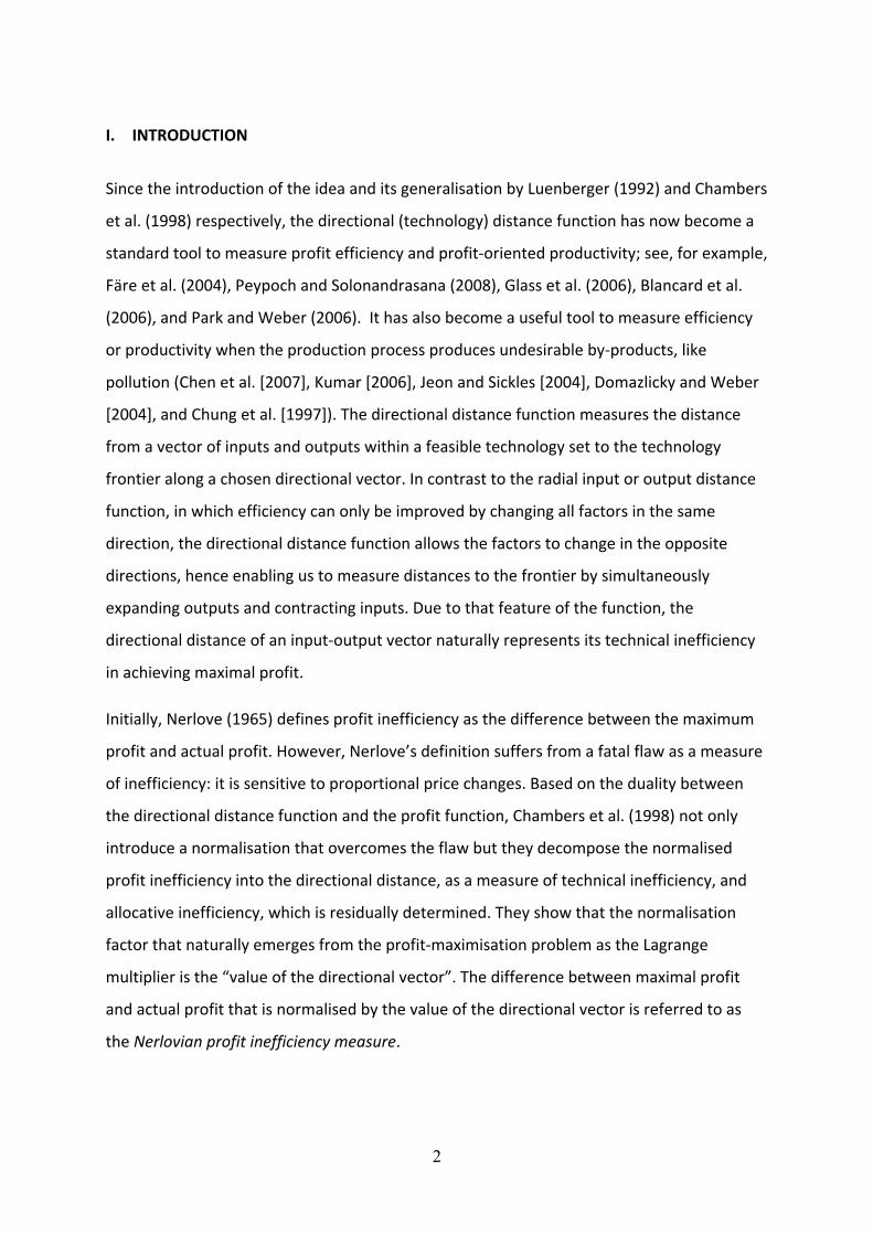
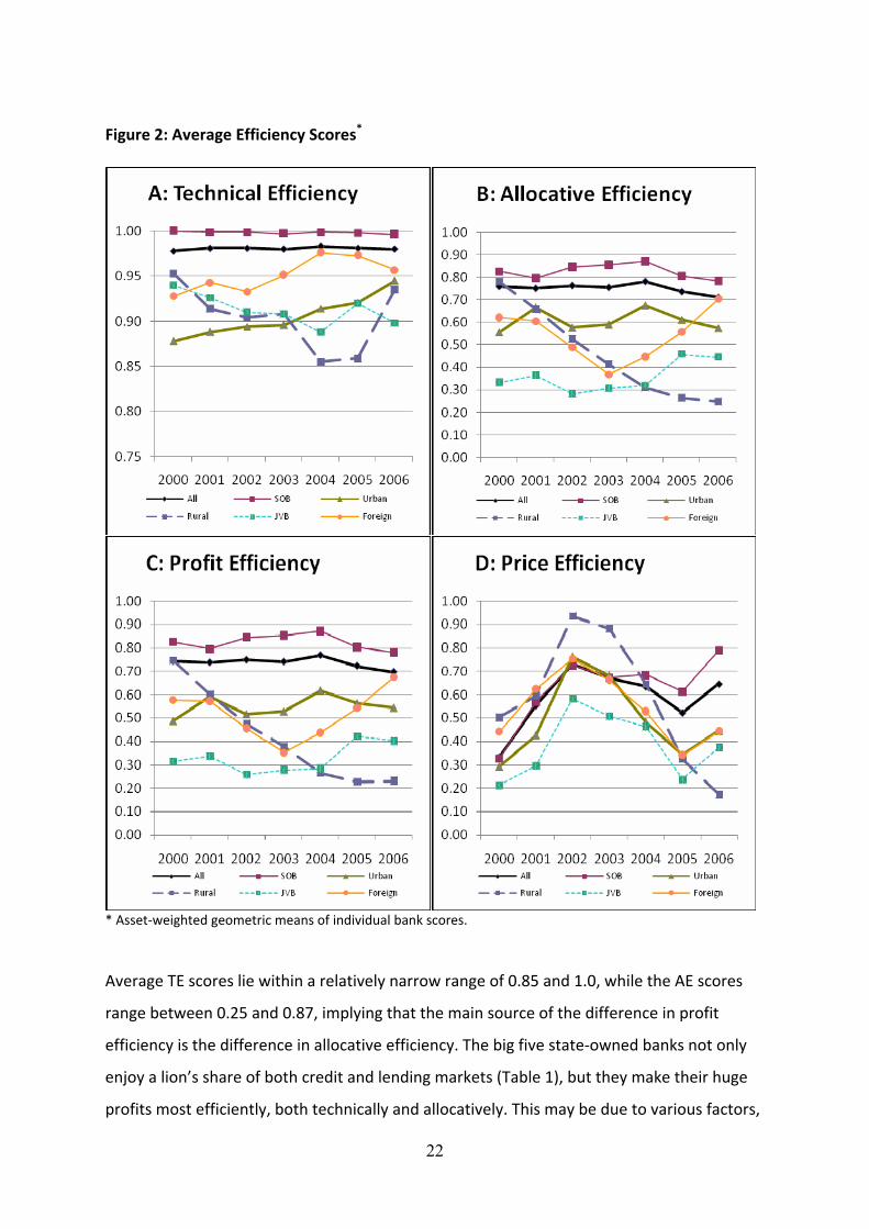
The graphs in Figure 2 show asset‐weighted geometric average technical efficiency (TE), 

allocative efficiency (AE), profit efficiency (PE), and price efficiency (PRE) scores for all and 

subgroups of banks in each year, with the capital‐adequacy constraint and the deposit 

constraint imposed on domestic banks and foreign banks respectively. There are 19 cases 

out of the 273 (39 domestic banks times 7 years) LP problems for directional distance where 

the bank in question violates the capital‐adequacy regulation with the ratio of equity capital 

to risk‐weighted assets falling below 8%. Of the 19 violations, 13 have been committed by 

SOBs, implying that the penalty fines imposed by the regulator have not been heavy enough 

to deter big banks from violating the regulation. Directional distances for those 19 cases 

have been set to zero, implying that the banks involved are technically efficient.7 Further, in 

4 cases out of those 19 cases, actual profit is higher than the maximum profit attainable 

under given prices. The banks in those cases are assumed to be allocatively efficient. 

 

                                                            5 The econometrics software program Shazam V10 (Whistler et al. 2004) has been used for the computation. A few instances of “computer cycling” were encountered during the computation, but they could be easily overcome by changing the units of measurement. See Gass and Vinjamuri (2004) for more details on computer cycling in LP problems. 

6 See, for example, Park and Weber (2006), and Tulkens and Vanden Eeckaut (1995). 7 In fact, the directional distances for those cases are zero except only for four cases when the capital‐adequacy constraint is excluded. Even for those four cases, the maximum value is only 0.06. 

22

Figure 2: Average Efficiency Scores*  

 * Asset‐weighted geometric means of individual bank scores. 

 

Average TE scores lie within a relatively narrow range of 0.85 and 1.0, while the AE scores 

range between 0.25 and 0.87, implying that the main source of the difference in profit 

efficiency is the difference in allocative efficiency. The big five state‐owned banks not only 

enjoy a lion’s share of both credit and lending markets (Table 1), but they make their huge 

profits most efficiently, both technically and allocatively. This may be due to various factors, 

23

including the advantages of being owned by the state and having a relatively long history 

and thus have a better market base. Joint‐venture banks and rural banks are performing 

poorly in both technical efficiency and allocative efficiency when compared with the other 

types of banks. Although joint‐venture banks and foreign banks are structurally similar, in 

terms of input‐out mix and profit‐equity capital ratio, foreign banks are making profits much 

more efficiently than joint‐venture banks. Foreign banks are also consistently more 

technically efficient than urban banks. They used to be less allocatively efficient than urban 

banks, but even allocatively have they become more efficient recently. The rapid 

deterioration in the profit efficiency of rural banks is conspicuous. Only recently have they 

improved technical efficiency but their allocative efficiency continued to deteriorate. This 

may be due to the fact that rural banks are basically carrying out traditional banking 

businesses and they are slow and have limited resources in adopting new technology and 

businesses. A statistic supporting that interpretation is the low share of revenue generated 

from off‐balance‐sheet items for rural banks (7% compared with 14%‐18% for other non‐

state‐owned banks).  

 

As mentioned in Section II, we also calculated price efficiency (PRE) scores to compare 

banks’ abilities to secure the most profitable price ratios. In each year, each bank’s profit‐

maximisation problem, (20), has been solved with each of the actual 56 price vectors faced 

by all banks in that year. Then, the maximum profit achievable among the 56 price vectors is 

regarded as πm, in (10)‐(11), for the bank in question in the corresponding year. Once λ2 is 

obtained, the price efficiency score is computed using (12). Panel D of Figure 2 shows PRE 

scores. While they change widely over the years, they are not much different across sub‐

groups. Joint‐venture banks are consistently less efficient than the other groups of banks, 

indicating that they have difficulty in securing profitable input and output prices. Rural 

banks surprisingly performed well in securing most profitable prices in the early years, but 

their performance has drastically deteriorated in more recent years.  

 

The efficiency scores estimated without imposing the capital‐adequacy and deposit 

constraints are not separately tabulated to save space. Imposing the capital‐adequacy 

constraint does not have effect on the technical efficiency of domestic banks in most cases, 

24

and even for the few cases where that has effect the largest difference is only 0.008. This 

implies that in most cases the directional vector faces a facet of the technical frontier other 

than the one that is formed by the capital‐adequacy constraint. Imposing the capital‐

adequacy constraint causes some changes in the allocative scores of domestic banks, with 

the mean absolute change being 0.025.8 

 

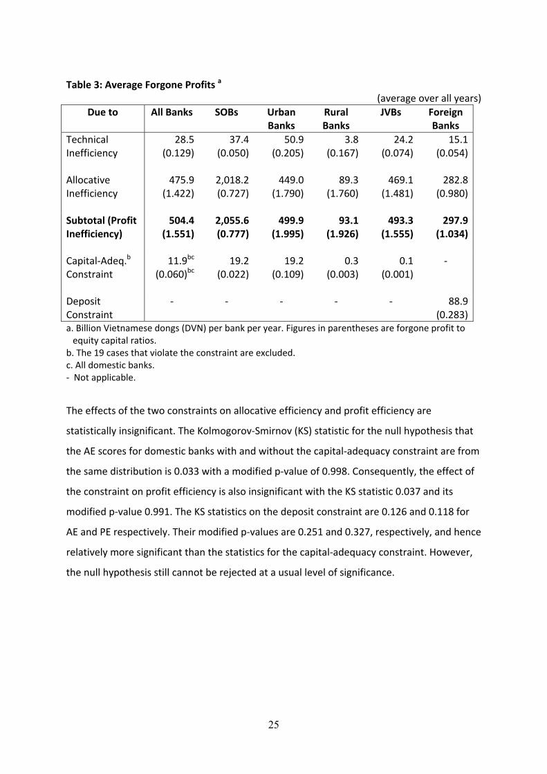
Table 3 reports average potential profits per bank per year that have been forgone due to 

inefficiencies and the regulations. The figures in parentheses are forgone profits as a 

multiple of equity capital. On average, potential profit forgone due to allocative inefficiency 

is almost seventeen times that lost due to technical inefficiency, which is an observation 

consistent with the high technical and the low allocative efficiency scores that have been 

noted above. As a group, all banks could have increased their aggregate yearly profit by 

DVN1,596b on average if all banks were technically efficient and by further DVN26,650b if 

they were allocatively efficient. If the capital‐adequacy constraint were removed, domestic 

banks’ maximum potential profit would increase by DVN11.9b per bank per year. This figure 

is much smaller than the potential increase in the maximum profit a foreign bank could 

achieve (DVN88.9b) if the deposit regulation were abolished. As a group, the 17 foreign 

banks’ aggregate maximum profit would have increased by DVN1,511b per year on average.  

A caveat for the foregoing interpretations is that the estimates have not taken into account 

possible constraints, such as limited resources or demand that could inhibit the banks from 

being technically and/or allocatively efficient.   

 

                                                            8 Note that imposing an additional constraint cannot decrease TE but it may decrease AE.  

25

Table 3: Average Forgone Profits a 

(average over all years) Due to  All Banks  SOBs  Urban 

Banks Rural Banks 

JVBs  Foreign Banks 

Technical Inefficiency  

28.5 (0.129) 

37.4(0.050)

50.9(0.205)

3.8(0.167)

24.2 (0.074) 

15.1(0.054)

Allocative Inefficiency  

475.9 (1.422) 

2,018.2(0.727)

449.0(1.790)

89.3(1.760)

469.1 (1.481) 

282.8(0.980)

Subtotal (Profit Inefficiency)  

504.4 (1.551) 

2,055.6(0.777)

499.9(1.995)

93.1(1.926)

493.3 (1.555) 

297.9(1.034)

Capital‐Adeq.b Constraint  

11.9bc 

(0.060)bc 19.2

(0.022)19.2

(0.109)0.3

(0.003)0.1 

(0.001) ‐ 

Deposit Constraint 

‐  ‐  ‐  ‐  ‐  88.9(0.283)

a. Billion Vietnamese dongs (DVN) per bank per year. Figures in parentheses are forgone profit to equity capital ratios. 

b. The 19 cases that violate the constraint are excluded. c. All domestic banks. ‐  Not applicable.  

The effects of the two constraints on allocative efficiency and profit efficiency are 

statistically insignificant. The Kolmogorov‐Smirnov (KS) statistic for the null hypothesis that 

the AE scores for domestic banks with and without the capital‐adequacy constraint are from 

the same distribution is 0.033 with a modified p‐value of 0.998. Consequently, the effect of 

the constraint on profit efficiency is also insignificant with the KS statistic 0.037 and its 

modified p‐value 0.991. The KS statistics on the deposit constraint are 0.126 and 0.118 for 

AE and PE respectively. Their modified p‐values are 0.251 and 0.327, respectively, and hence 

relatively more significant than the statistics for the capital‐adequacy constraint. However, 

the null hypothesis still cannot be rejected at a usual level of significance. 

 

26

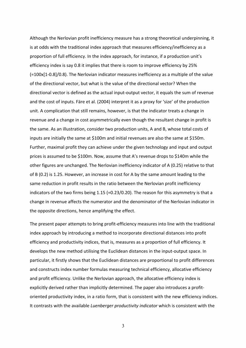
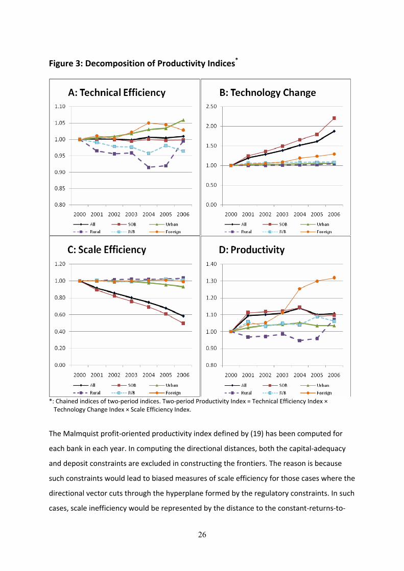
Figure 3: Decomposition of Productivity Indices* 

 

 *: Chained indices of two‐period indices. Two‐period Productivity Index = Technical Efficiency Index × Technology Change Index × Scale Efficiency Index. 

 

The Malmquist profit‐oriented productivity index defined by (19) has been computed for 

each bank in each year. In computing the directional distances, both the capital‐adequacy 

and deposit constraints are excluded in constructing the frontiers. The reason is because 

such constraints would lead to biased measures of scale efficiency for those cases where the 

directional vector cuts through the hyperplane formed by the regulatory constraints. In such 

cases, scale inefficiency would be represented by the distance to the constant‐returns‐to‐

27

scale (CRS) frontier from the frontier formed by the regulatory constraint instead of the 

variable‐returns‐to‐scale (VRS) frontier formed by the input‐output constraints.  The 

productivity indices are decomposed into technical efficiency index (TEI), technology change 

index (TCH), and scale efficiency index (SEI) as shown in (19). The graphs in Figure 3 show 

asset‐weighted geometric averages of those component indices as well as the productivity 

indices for different groups of banks. The time‐series of the indices over the sample period, 

with year 2000 as the base period, are constructed by chaining two‐period indices. The first 

three panels show that the group of SOBs had experienced the fastest improvement in the 

technology, the worst deterioration in scale efficiency, and little change in technical 

efficiency over the sample period among the groups of banks. Given their huge size and 

funds available for technology improvement, it is not surprising to observe the fastest 

growth in technology from the group of SOBs. There had been little change in their technical 

efficiency simply because all banks in that group operated at full (or near full) technical 

efficiency in most years. On the other hand, their scale efficiency had deteriorated by more 

than40% over the seven‐year period. As none of the SOBs are operating at an increasing 

returns to scale (Table 4), the ever decreasing SEI implies that the scales of SOBs are over 

the most optimal scale and had been growing further and further beyond that scale, 

becoming less and less scale efficient. The overall score card, in terms of productivity 

improvement, is the most outstanding for the group of foreign banks, which had improved 

productivity by more than 30% over the period. Their scale had been always close to the 

optimum, while technical efficiency and technology had improved significantly. Rural banks 

used to be the most technically inefficient among the groups. However, they ended the 

sample period with the third highest productivity index, after SOBs and foreign banks, 

thanks to the significant improvement in technical efficiency in the last period and steadily 

improving scale efficiency. 

 

28

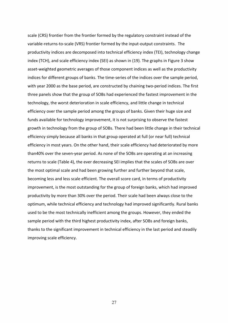
Table 4: Numbers and Proportions of IRS, DRS and MPSS Cases    SOB  Urban  Rural  JVB  Foreign  All Banks 

IRS  0 (0.0%) 

61 (43.6%) 

46 (65.7%) 

2 (7.1%) 

18 (15.1%) 

127 (32.4%) 

DRS  26 (74.3%) 

68 (48.6%) 

20 (28.6%) 

22 (78.6%) 

74 (62.2%) 

210 (53.6%) 

MPSS  9 (25.7%) 

11 (7.8%) 

4 (5.7%) 

4 (14.3%) 

27 (22.7%) 

55 (14.0%) 

All  35  140  70  28  119  392  

Table 4 reveals that in about two‐thirds of the cases the SOBs are operating in an area of 

decreasing returns to scale implying that their operating scales are bigger than an optimal 

level. A similar proportion (79%) of JVBs and 62% of foreign banks are also operating in an 

area of decreasing returns to scale. On the other hand, a majority (66%) of rural banks have 

a room to improve productivity by increasing their scales. Urban banks are almost evenly 

split between increasing returns to scale (44%) and decreasing returns to scale (49%). The 

groups of SOBs and foreign banks have the largest proportions (26% and 23% respectively) 

of cases that are operating at the most productive scale size (MPSS).   

 

V. CONCLUSIONS 

 

We have introduced a new approach to constructing technical efficiency, allocative 

efficiency, and profit efficiency indices using directional distances. Unlike the available 

indicator approaches that are based on differences, the new indices are based on ratios 

between distances, hence making interpretations more sensible. We have also decomposed 

the profit‐oriented Malmquist productivity index into scale‐efficiency index, pure technical‐

efficiency index and technology‐change index in a way that is fully consistent with the new 

ratio‐type efficiency indices. In doing so, we have explicitly shown how to handle infeasible 

linear‐programming problems when the directional distance of an input‐out vector is 

measured against the technology frontier in another period.  

 

Then, the new methods have been applied to an analysis of the Vietnamese banking sector. 

The analysis shows that the five largest state‐owned banks are most technically and 

29

allocatively efficient, but their scale efficiency is the lowest among the different groups and 

it consistently deteriorates over the sample period. The most successful group, in terms of 

productivity improvement, appears to be the group of foreign banks. Their technical 

efficiency and the growth rate of technology are better than any other groups except SOBs, 

resulting in the highest improvement in overall productivity, including SOBs, over the 

sample period. For all groups, the main source of profit inefficiency is allocative inefficiency. 

When measured in terms of forgone profits, the effect of allocative inefficiency is more than 

sixteen times the effect of technical inefficiency. The effects of the two regulatory 

constraints are found to be insignificant both in size and statistical sense.  

 

Policy implications of the findings are that i) Policies that would result in the expansion of 

the size of SOBs would lead to significant decrease in their productivity due to deteriorating 

scale efficiency; ii) To support the viability of rural banks, measures should be directed 

towards promoting expansions of their business areas and sizes, possibly through mergers, 

so that both allocative efficiency and scale efficiency can be improved; iii) Main reasons for 

the poor performance of joint‐venture banks, especially compared with foreign banks, 

should be carefully analysed and relevant measures should be taken to improve 

productivity; iv) The capital‐adequacy constraint does not impose significant restriction on 

productivity, and hence it should be more strictly applied to enhance the stability of the 

financial system.  

30

REFERENCES  Blancard, Stephane, Jean‐Philippe Boussemart, Walter Briec, and Kristiaan Kerstens (2006), “Short‐ and Long‐Run Credit Constraints in French Agriculture: A Directional Distance Function Framework Using Expenditure‐Constrained Profit Functions”, American Journal of Agricultural Economics 88(2), 351‐364  Caves, Douglas W., Laurits R. Christensen, and W. Erwin Diewert (1982), “The Economic Theory of Index Numbers and the Measurement of Input, Output, and Productivity”, Econometrica 50(6), 1393‐1414  Chambers, Robert G., Y. Chung, and R. Färe (1998), “Profit, Directional Distance Functions, and Nerlovian Efficiency”, Journal of Optimization Theory and Applications 98(2), 351‐364  Chambers, Robert G., Rolf Färe, and Shawna Grosskopf (1996), “Productivity Growth in APEC Countries”, Pacific Economic Review 1(3), 181‐190    Chen, Po‐Chi, Ming‐Miin Yu, Ching‐Cheng Chang, and Shih‐Hsun Hsu (2007), “Productivity Change in Taiwan’s Farmers’ Credit Unions: A Nonparametric Risk‐Adjusted Malmquist Approach”, Agricultural Economics 36(2), 221‐231  Chung, Y., R. Färe, and S. Grosskopf (1997), “Productivity and Undesirable Outputs: A Directional Distance Function Approach”, Journal of Environmental Management 51, 229‐240  Domazlicky, Bruce R. and William L. Weber (2004), “Does Environmental Protection Lead to Slower Productivity Growth in the Chemical Industry?”, Environmental and Resource Economics 28(3), 301‐324  Färe, Rolf, Shawna Grosskopf, and William L. Weber (2004), “The Effect of Risk‐Based Capital Requirements on Profit Efficiency in Banking”, Applied Economics 36, 1731‐1743   Gass, Saul I., and Sasirekha Vinjamuri (2004), “Cycling in Linear Programming Problems”, Computers & Operations Research 31, 303‐311   Glass, J.C., G. McCallion, D.G. McKillop, and K. Stringer (2006), “A ‘Technically Level Playing‐Field’ Profit Efficiency Analysis of Enforced Competition between Publicly Funded Institutions”, European Economic Review 50(6), 1601‐26  Jeon, Byung M. and Robin C. Sickles (2004), “The Role of Environmental Factors in Growth Accounting”, Journal of Applied Econometrics 19(5), 567‐591  Kumar, Surender (2006), “Environmentally Sensitive Productivity Growth: A Global Analysis Using Malmquist‐Luenberger Index”, Ecological Economics 56(2), 280‐293  

31

Luenberger, D.G. (1992), “New Optimality Principles for Economic Efficiency and Equilibrium”, Journal of Optimization Theory and Applications 75(2), 221‐264    Nerlove, M. (1965), Estimation and Identification of Cobb‐Douglas Production Functions, Rand McNally Co., Chicago  Nguyen, Viet Hung (2007), “Measuring Efficiency of Vietnamese Commercial Banks: An Application of Data Envelopment Analysis (DEA)”, in Khac Minh Nguyen and Thanh Long Giang (ed.), Technical Efficiency and Productivity Growth in Vietnam, Publishing House of Social Labour, Tokyo   Park, Kang H., and William L. Weber (2006), “A Note on Efficiency and Productivity Growth in the Korean Banking Industry, 1992‐2002”, Journal of Banking and Finance 30, 2371‐2386  Peypoch, Nicolas, and Bernardin Solonandrasana (2008), “Aggregate Efficiency and Productivity Analysis in the Tourism Industry”, Tourism Economics 14(1), 45‐56  Ray, S.C. (2008), “The Directional Distance Function and Measurement of Super‐Efficiency: An Application to Airline Data”, Journal of the Operational Research Society 59, 788‐797  Tulkens, Henry, and Philippe Vanden Eeckaut (1995), “Non‐parametric Efficiency, Progress and Regress Measures for Panel Data: Methodological Aspects”, European Journal of Operational Research 80(3), 474‐499   Whistler, Diana, Kenneth J. White, S. Donna Wong, and David Bates (2004), SHAZAM Econometrics Software Version 10 User’s Reference Manual, Northwest Econometrics Ltd., Vancouver