Profit Maximization Aircraft Design Project Final Report

University of Michigan

Department of Mechanical Engineering

Yu-Hung Ho Chun-Min Ho

Chun-Shiang Lin Shih-Kang Peng

Abstract

Passenger capacity and operational cost of the aircraft was considered for the overall profit model. The overall system was broken down into four disciplines, seat arrangement (SA), cold air unit (CAU), fuselage structure (FSU), and the turbofan engines (TFE). The subsystems were optimized individually as well as collectively. The optimal results showed differences because subsystems have conflict in desired optimizer, such as T04 in CAU and TFE subsystems, and the Lc and Wc in the SA, FSU, and CAU subsystems. TFE subsystem works to minimize the specific fuel consumption (SFC) and the value decreased from 55.3E-6 kg/N-s in the individual optimization to a value for 7.32E-6 kg/N-s in the combined system. Both the CAU and FSU subsystem works to minimize the weight and CAU increased from 1034 kg to 1300 kg, while FSU decreased from 1330 kg to 1266 kg. SA works to maximize the passenger capacity and it decreased from 216 to 137. From the results it was clear that in the conflict of the interest of each subsystem, TFE subsystem in the latter part of the objective function dominates the former in the individual optimizer SA capacity. We see the capacity was compromised for a better SFC value.

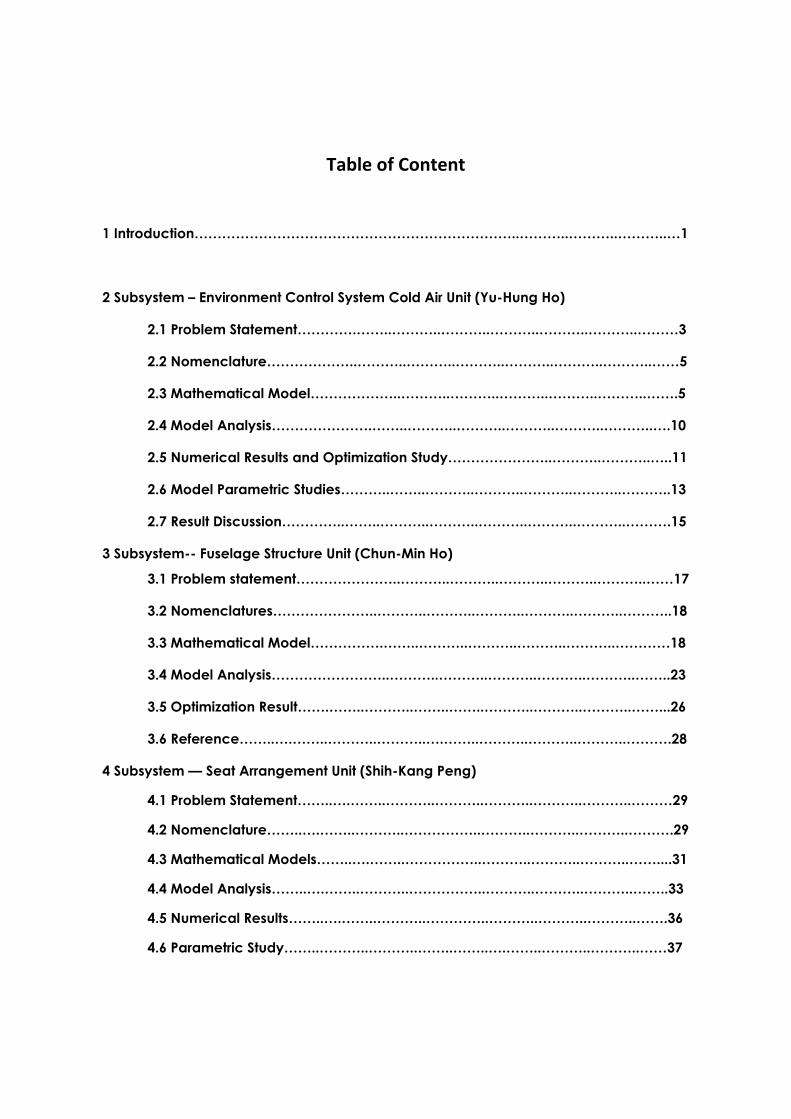
Table of Content

1 Introduction……………………………………………………………..………..………..………..…1

2 Subsystem – Environment Control System Cold Air Unit (Yu-Hung Ho)

2.1 Problem Statement………….……..………..………..………..………..………..………3

2.2 Nomenclature………………..………..………..………..………..………..………..……5

2.3 Mathematical Model………………..………..………..………..………..………..…….5

2.4 Model Analysis………………….……..………..………..………..………..………..….10

2.5 Numerical Results and Optimization Study…………………..………..………..…..11

2.6 Model Parametric Studies………..……..………..………..………..………..………..13

2.7 Result Discussion…………..……..………..………..………..………..………..……….15

3 Subsystem-- Fuselage Structure Unit (Chun-Min Ho)

3.1 Problem statement…………………..………..………..………..………..………..……17

3.2 Nomenclatures…………………..………..………..………..………..………..………..18

3.3 Mathematical Model…………….……..………..………..………..………..…………18

3.4 Model Analysis……………………..………..………..………..………..………..……..23

3.5 Optimization Result…….……..………..……..……..………..………..………..……...26

3.6 Reference……..….……..………..………..….……..………..………..………..……….28

4 Subsystem — Seat Arrangement Unit (Shih-Kang Peng)

4.1 Problem Statement……..….……..………..………..………..………..………..………29

4.2 Nomenclature……..….……..………..……………..………..………..………..……….29

4.3 Mathematical Models……..….……..……………..………..………..………..……....31

4.4 Model Analysis……..….……..………..……………..………..………..………..……..33

4.5 Numerical Results……..….……..………..…………..………..………..………..…….36

4.6 Parametric Study……..………..………..……..……..….……..………..………..……37

4.7 Discussion……..….……..………..………..…….……..………..………..………..…….38

4.8 Reference……..….……..………..………..……..……..………..………..………..……38

5 Subsystem – Turbofan Engine (Chun-Shiang Lin)

5.1 Problem Statement……..………..……….……..………..………..………..…….…….39

5.2 Nomenclature……..………..………..………..………..………..………..………..……39

5.3 Mathematical Model……..………..………..….……..………..………..………..……41

5.4 Model Analysis……..………..………..………………..………..………..………..……46

5.5 Numerical Results……..………..………..……...……..………..………..………..…...48

5.6 Result discussion…………..………..………...………..………..………..………..……50

5.7 Reference…………..………..………..………..………..………..………..………..……51

6 All-in-One System

6.1 Problem Statement……..………..………..…….……..………..………..………..…..52

6.2 Nomenclature…………..………..………..…..………..………..………..………..…..53

6.3 Mathematical Model…………..………..…...………..………..………..………..…..54

6.4 AIO Model Integration………..………….…..……..………..………..………..……..58

6.5 Result Analysis……..………..………..………….……..………..………..………..…..59

Appendix

Appendix A…………………………………..……..………..………..………..………..….60

1

1 Introduction Airliners are the fastest and yet most expensive mode of commercial

transportation. Every year, approximately 1.5 billion passengers board airliners.

Currently there are about 50 competitive airline companies around the world. In

this saturated market, the profitability in the industry varied from reasonable to

devastating, and thus maximizing the profit for each flight is critical. We broke

down the subsystems into four subsystems as the following.

1. Minimize fuel consumption from the cabin cold air unit

2. Minimize fuselage structure weight

3. Maximizing the number of passengers through seating arrangement

4. Minimize turbofan engine fuel consumption

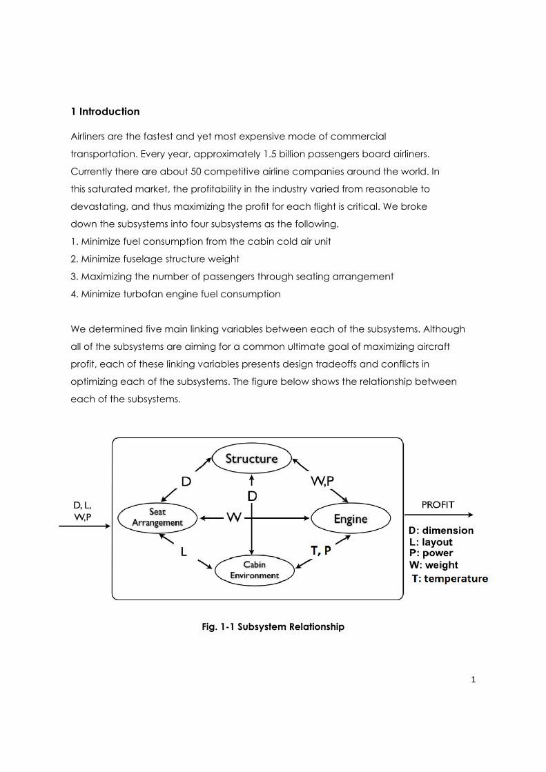
We determined five main linking variables between each of the subsystems. Although

all of the subsystems are aiming for a common ultimate goal of maximizing aircraft

profit, each of these linking variables presents design tradeoffs and conflicts in

optimizing each of the subsystems. The figure below shows the relationship between

each of the subsystems.

Fff

Fig. 1-1 Subsystem Relationship

2

A smaller fuselage diameter is desired for structural weight, as well as the

minimal CAU power consumption. These will result in increased aircraft profit.

However, for a small fuselage diameter, the number of passenger per flight will

be compromised, which would lead to decreased profit. An optimization

algorithm must be performed in order to achieve the optimal diameter of the

fuselage to maximize the profit. For increased turbofan engine fuel efficiency,

the desired post-compressor stage temperature is as high as possible, subject to

turbine blade thermal tolerance. The cold air unit however, desires a lower

temperature so the refrigeration cycle compressor work input can be minimized.

Therefore an optimal post-compressor stage temperature is needed to realize

maximum fuel efficiency. To supply fresh air for the cabin, a portion of engine

compressed air must be bled off, which would result in increased fuel

consumption.

The complexity of this profit optimization problem is revealed due to these linking

variable conflicts. The optimal variables for each of the subsystem will not

necessarily be the optimal values for the all-in-one system optimization. The

degrees of influence that each of the subsystems have on the overall aircraft

profit are also unknown, therefore it is worthwhile to explore this problem further.

A complicated optimization analysis is needed to achieve the maximized

aircraft profit.

3

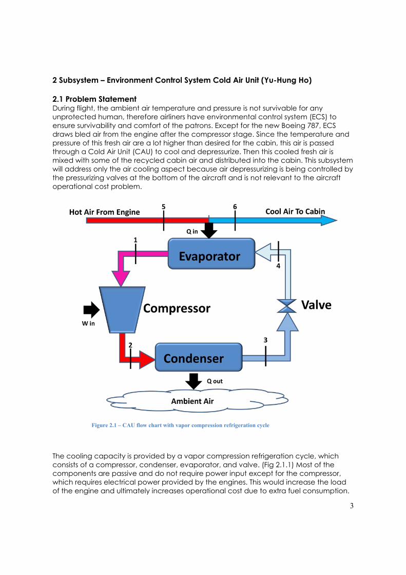
2 Subsystem – Environment Control System Cold Air Unit (Yu-Hung Ho) 2.1 Problem Statement During flight, the ambient air temperature and pressure is not survivable for any unprotected human, therefore airliners have environmental control system (ECS) to ensure survivability and comfort of the patrons. Except for the new Boeing 787, ECS draws bled air from the engine after the compressor stage. Since the temperature and pressure of this fresh air are a lot higher than desired for the cabin, this air is passed through a Cold Air Unit (CAU) to cool and depressurize. Then this cooled fresh air is mixed with some of the recycled cabin air and distributed into the cabin. This subsystem will address only the air cooling aspect because air depressurizing is being controlled by the pressurizing valves at the bottom of the aircraft and is not relevant to the aircraft operational cost problem. The cooling capacity is provided by a vapor compression refrigeration cycle, which consists of a compressor, condenser, evaporator, and valve. (Fig 2.1.1) Most of the components are passive and do not require power input except for the compressor, which requires electrical power provided by the engines. This would increase the load of the engine and ultimately increases operational cost due to extra fuel consumption.

Figure 2.1 – CAU flow chart with vapor compression refrigeration cycle

4

Cycle component sizes are also important for the fuel cost, and the tradeoff for more efficient components is weight. For aircraft, weight is very important due to the high cost jet fuels. To simplify this subsystem model and avoid expensive calculation, only compressor sizing will be considered. Evaporator and condenser sizing may be included in the future. The weight of the compressor also adds load to the engine, which increases the fuel consumption. A common refrigerant R-134a is picked for the working fluid because there are a wide variety of off-the-shelf compressors offered by the sellers that uses R-134a. The amount of R-134a would also be taken into account. The more refrigerant the aircraft has to carry would lead to an increase in fuel consumption. However, the less refrigerant CAU has the less fresh air the CAU is able to provide for the cabin. Regulation requires at least 50% of the cabin air must be fresh. Amount of air is related to amount of refrigerant in the CAU by first law of thermodynamics. Assuming no heat loss between the air line and the evaporator of the CAU, the heat loss in the air line is exactly the heat absorbed by the evaporator.

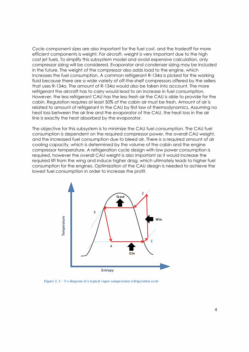
The objective for this subsystem is to minimize the CAU fuel consumption. The CAU fuel consumption is dependent on the required compressor power, the overall CAU weight, and the increased fuel consumption due to bleed air. There is a required amount of air cooling capacity, which is determined by the volume of the cabin and the engine compressor temperature. A refrigeration cycle design with low power consumption is required, however the overall CAU weight is also important as it would increase the required lift from the wing and induce higher drag, which ultimately leads to higher fuel consumption for the engines. Optimization of the CAU design is needed to achieve the lowest fuel consumption in order to increase the profit.

Figure 2. 2 – T-s diagram of a typical vapor compression refrigeration cycle

5

2.2 Nomenclature = mass of the air flow (kg)

= mass of the refrigerant flow (kg)

= mass of the compressor (kg)

= temperature of the bled air ( C)

= temperature of the cabin ( C)

= temperature at state i, for i = 1, 2, 3, 4 ( C)

= pressure at state i, for i = 1, 2, 3, 4 (kPa)

= specific enthalpy at state i, for i = 1, 2, 3, 4, 5, 6 (kJ/kg)

= specific entropy at state i, for i = 1, 2, 3, 4 (kJ/kg-­‐K)

= vapor quality at state i, for i = 1, 2, 3, 4 (kg/kg)

= compressor input work rate (kJ)

= Nominal Engine Energy Output (kJ)

= Maximum take-off weight (kg)

= Cabin volume (m3)

2.3 Mathematical Model 2.3.1 Refrigeration Cycle Thermodynamics Referring to figure 2.1.2, the refrigeration cycle can be broken down into 4 different states. Since R-134a behaves very differently from superheated vapor to saturated vapor, several assumptions will be made to simplify the model and reduce the computational cost. For optimal compressor rated performance, states 1 and 2 will be assumed to be in the superheated region. The compressor will also be assumed isentropic. Also for the best compressor performance, state 3 will be assumed to be at the saturated liquid state and state 4 will be inside the saturated region with 25% vapor quality. Evaporators and condensers are also assumed to be isobaric. 2. 3.2 Objective function

= + + × + ( ) × The objective function is the sum of the increased engine load due to the operation of the CAU. This includes, required compressor energy, which is taken from off-the-shelf compressor data. Although it is most adequate to treat such a problem with discrete optimization, but there are abundant of compressor models available, we will assume that the compressor specification that is obtained from this optimization analysis can be achieved by some compressor model. Using thermodynamic equations, the required input work for a compressor is given by the following equation:

6

= ( )

A neural network model based on specifications of a collection of compressor models is built with , , and as inputs and as outputs.

= ( , , )

Increased engine load also includes the required engine energy output due to the weight of CAU. With increased aircraft weight, higher lift is required. To keep wing area, aspect ratio, and cruise velocity, the coefficient of lift must increase by the same amount. With increased coefficient of lift, the coefficient of induced drag increases as well. The coefficient of induced drag increases as the square of coefficient of lift so we see that the increased engine load is proportional to the square of the percentage of CAU weight with respect to the MTOW. The increased weight function (IW) is given as the following, where g is the gravitational acceleration.

+ = (1 ++

)

The increased engine load that is due to air bleeding off of the engine compressor can be modeled by data given on a study done by Hunt et. al. Figure 2.1.3 shows the relationship between percent of bleed air, which is calculated by the percentage of fresh air with respect to the cabin air volume, and the percentage of increased fuel consumption.

Figure 2. 3 – Bleed air percentage vs increased fuel consumption percentage

7

The modern turbofan data with 5:1 bypass ratio most represents the A320 engines. The increased fuel consumption is proportional to the nominal engine energy output. The following functional relationship can be derived for increased fuel consumption, where

is the density of cabin air.

( ) = 0.5 1.56 + 0.8

The relationship between and is derived. Using energy conservation for heat transfer and ideal gas approximation for the air line, the relationship is shown below. is the air specific heat with constant pressure.

( ) = ( )

Metamodels will be created for the following thermodynamic properties and relations.

[ , ] = ( , )

= ( , ) = ( , )

2.3.3 Design Variables and Parameters

Design Variable Definition Typical Range Compressor

Inlet temperature ( C)

20 < <

Compressor

outlet temperature ( C)

< < 50

Compressor

Inlet pressure (kPa)

60 < < 2000

Mass of refrigerant (kg) 0 < < 2000

The state 1 and 2 temperature values are determined from the thermodynamic tables. No tabulated values are available outside of the typical range. R-134a property drastically changes outside of this range. State 1 pressure value range is also determined from the typical R-134a range. A very rough calculation was done for maximum value to determine the maximum value.

Table 2.1 – List of design variables with simple upper and lower bounds

8

Design Parameter Definition Typical Value Nominal engine energy

output (kJ) 120

Cabin volume (m3) 300

Maximum take-off weight (kg)

77111

Bled air temperature ( C) 680

The design parameters are taken from the A320 specification sheet. These parameters are also possible linking variables to other subsystems.

Design Constant Definition Typical Value Air specific heat (kJ/kg-­‐K) 1.012

Cabin air density (kg/m3) 1.2

Cabin air temperature ( C) 22

The cabin air temperature is set at a level that the CAU must achieve for human comfort. The cabin air density is evaluated at the cabin air temperature. Assuming constant specific heat for the air, the typical value is given above.

2.3.4 Constraints Model Validity Constrains:

The R-134a superheated tables show that as pressure increase the saturation temperature increases as well. There are upper and lower bounds for allowable superheated vapor temperature with the corresponding pressure. The upper and lower bound temperatures were taken with the respective pressures and a cubic polynomial fit was applied to it to create the temperature constrain with respect to the pressure. These constrains ensures R-134a remains in superheated vapor state, otherwise condensation and chemical disassociations might occur and the mathematical problem becomes invalid.

:   ( ) 0   :   ( ) 0 :   ( ) 0   :   ( ) 0

Where,

( ) = 88.3 + 0.898 3.58 9.55

Table 2.2 – List of parameters with simple upper and lower bounds

Table 2.3 – List of design constants with simple upper and lower bounds

9

( ) = 30.66 + 0.133 7.24 + 1.58

Since isentropic relations are needed to obtain the thermodynamic properties at state 2, similar relationships between pressure and entropy are also needed to ensure the feasibility of property existence.

:   ( ) 0   :   ( ) 0

Where,

( ) = 1.28 + 2.14 6.49 + 3.77 ( ) = 0.94 + 3.28 8.33 + 4.43

Physical Constrains:

By definition, compressor must increase the flow pressure. Also the flow temperature cannot decrease through a compressor.

:     0 :     0

To ensure the normal behaviors of R-134a, pressure bounds are set.

:    60 0 :     2000 0

Practical Constrains:

Due to passenger comfort level, the fresh air entering the cabin must take up at least 50% of the cabin volume. With the air and refrigerant mass relation described above, the following constrains the mass of refrigerant.

:    12

( )( ) 0

2.3.5 Model Summary This subsystem aims to minimize required power consumption on the engines through designing a vapor compression refrigeration cycle with variables 1, 2, 1, .

min 1, 2, 1, = + + × + ( ) ×

Where,

= ( )

10

= ( , , )

+ = (1 ++

)

( ) = 0.5 1.56 + 0.8

( ) = ( ) [ , ] = ( , )

= ( , ) = ( , )

Subject to,

:   ( ) 0   :   ( ) 0 :   ( ) 0   :   ( ) 0 :     0

:   ( ) 0   :   ( ) 0 :    60 0 :     2000 0 :     0

:    12

( )( ) 0

Where, ( ) = 88.3 + 0.898 3.58 9.55

( ) = 30.66 + 0.133 7.24 + 1.58 ( ) = 1.28 + 2.14 6.49 + 3.77 ( ) = 0.94 + 3.28 8.33 + 4.43

2.4 Model Analysis 2.4.1 Monotonicity Analysis and Well-Boundedness Some parts of the objective function and constraints have thermodynamic property relations embedded inside, modeled using neural network, so the simple monotonicity analysis can be very complicated. However monotonicity analysis could still reveal some mathematical characteristics and well-boundedness of this model on the other parts of the model that has more apparent monotonicity. The following is the monotonic table. The objective function has been broken down to the three main parts and the overall objective function is examined. Though P2 and s1 are not exactly variables, they are the indirect linking variables between some of the relations, so they will be included in this table.

11

  T1   T2   P1   P2   s1   mref  Win   -­‐   +         +  IW   U   U   U       +  IFC   +     -­‐       +  f   U   U   U       +                g1     +     +      g2     -­‐     +      g3   +     +        g4   -­‐     +        g5   +   -­‐          g6         -­‐   +    g7         +   -­‐    g8       -­‐        g9         +      g10       +   -­‐      g11   -­‐     +       -­‐  

As mentioned before, the behavior of temperature and pressure values are not obvious but it is clear that mref is monotonically increasing with the objective function. The only upper bound is g11, which we expect to be active.

Though the monotonicity of the other variables (T1, T2, P1, P2, s1) are not clear, we can see that each of the variables have an upper and lower bound, creating a bounded feasible domain. For the objective function variables, T1 is bounded below by g4 and g11, and above by g3 and g5. Therefore we expect that if T1 were to have monotonicity, one of the 4 would be active. T2 has lower bounds g2 and g5, and upper bound at g1. Similarly P1 has upper bounds at g3, g4, g10, and g11, with lower bound at g8. P2 and s1 are also bounded from above and below. This ensures a well-bounded feasible region.

2.5 Numerical Results and Optimization Study MATLAB function fmincon was used for optimization. Initial conditions were picked in the feasible domain. The optimal result is shown below.

x = -15.58 3.35 121.31 880.79

fval_a = 223.309

Table 2.4 – Objective function and constraint monotonicity table

12

The active constraints were identified to be g2, g4, and g11. The multipliers for each of the constraints were 2.34, 2.34, and 0.02 respectively. Fortunately we can immediate note that none of the multipliers are negative, this ensures the correct convergence and feasibility of the optimized solution.

Constraints g2 and g4 pertains to the temperature lower bound of the vapor compressor inlet and exit states. The model validity constraint specifies that the temperature of the superheated vapor cannot below a certain level for their respective pressure to ensure the superheated vapor behavior of the refrigerant. It seems like the optimized solution is staying at the floor of the temperature range for the given pressure. This phenomenon can be explained by the fact that as the operating temperature of a compressor increases, the cooling capacity tapers off so for the same temperature difference. From figure 2.1.2 we see that the isobaric lines have increasing slopes. Since the cooling capacity is given by the area under the isobaric curve (Tds), the area does not increase a whole lot with the increasing temperatures. Therefore the cooling capacity decreases with the same amount of pressure difference, with larger compressor required. This would lead to increased compressor weight. We see that the optimizer wants to stay at the lower side of the temperature bound. One might be tempted to have temperatures lower than the model validity constraint, however this would completely changed the refrigeration cycle physics, as the cycle being analyzed is vapor-compression refrigeration cycle, and thus requires the compression of refrigerant vapor. If the temperature were picked below the model validity constraint values, condensations might occur, and we would be dealing with multiphase refrigerant. Compressors typically do not operate efficiently with multiphase fluid. With g2 and g4 active, we see much similarity between the existing vapor-compression refrigeration cycle designs with compressor inlet very close to the vapor saturation point.

The multiplier for g11 is very close to 0, so it might seem debatable to say whether or not g11 is active due to numerical errors. However from monotonicity analysis, g11 is indeed active. g11 is the only constraint bounding the monotonic variable mref from below. This means that mref is at the lowest feasible point. We see that as mair decreases, the cooling capacity required decreases as well. This could be reflected either in decreased mref in the CAU or decreased compressor work, both of which result in decreased objective function value. To minimize fuel consumption due to operation of CAU, no cooling system necessary is ideal, however, because an aircraft must create a survivable and comfortable environment for the passengers, the ultimate minimum cannot be achieved. Regulation states that at least 50% of the cabin air must be fresh at any given time; the constraint g11 becomes an equality constraint.

Different sets of initial values were selected and the optimization analysis yields the same result. A number of initial value combinations were selected to test model robustness and see whether the optimizer is global or local. Extreme values were used in this case, a combination of lowest possible values and highest possible values were initialized. The table below shows a few of the starting points and the resulting objective function value.

13

x0 f

[-20, 50, 60, 1] 223.31

[-20, -10, 2000, 1] 223.31

[45, 50, 2000, 2000] 223.31

[-20, 50, 60, 2000] 223.31

[-20, -10, 2000, 1] 223.31

[25, 50, 60, 500] 223.31

There was one initial case noted where the optimum differs from the aforementioned result. When T1 and T2 values were initially equal to one another, the optimal result would yield the following:

x = 3.39 3.39 302.82 847.10

fval_a = 237.53

The result suggests constant temperature throughout the compressor. With the assumed isentropic modeling of this compressor, this would suggest constant enthalpy throughout the compressor as well. This suggests that no work input is required and renders the CAU useless. Perhaps constraint g5 should be set to be strictly less than 0 to avoid this bug.

2.6 Model Parametric Studies Two of the CAU subsystem parameters, namely Tbleed and Vcabin are possible linking variables to the other subsystems. Tbleed will depend on the post engine compressor stage air temperature, which depends on the engine design. Vcabin will depend on the structures subsystem. Parametric studies will be done on these two parameters to see potential effects of the optimized objective function value from the other subsystems.

The nominal value for Tbleed is 680 C, which is taken from the A320 engine specification sheet. Tbleed should not come close to Tcabin otherwise singularity will occur in the mair equation and g11. Plot below shows the optimized objective function value vs. Tbleed temperature.

Table 2.5 – List of random starting points and their respective converged objective function value

14

400 600 800 1000 1200 1400 1600 1800

223.3

223.35

223.4

223.45

obj f

unct

ion

Tbleed (c)

Tbleed Parametric study

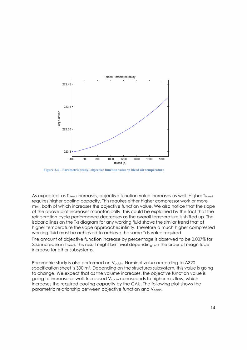
As expected, as Tbleed increases, objective function value increases as well. Higher Tbleed requires higher cooling capacity. This requires either higher compressor work or more mref, both of which increases the objective function value. We also notice that the slope of the above plot increases monotonically. This could be explained by the fact that the refrigeration cycle performance decreases as the overall temperature is shifted up. The isobaric lines on the T-s diagram for any working fluid shows the similar trend that at higher temperature the slope approaches infinity. Therefore a much higher compressed working fluid must be achieved to achieve the same Tds value required.

The amount of objective function increase by percentage is observed to be 0.007% for 25% increase in Tbleed. This result might be trivial depending on the order of magnitude increase for other subsystems.

Parametric study is also performed on Vcabin. Nominal value according to A320 specification sheet is 300 m3. Depending on the structures subsystem, this value is going to change. We expect that as the volume increases, the objective function value is going to increase as well. Increased Vcabin corresponds to higher mair flow, which increases the required cooling capacity by the CAU. The following plot shows the parametric relationship between objective function and Vcabin.

Figure 2.4 – Parametric study: objective function value vs bleed air temperature

15

200 250 300 350 400 450 500 550 600 650

223.24

223.26

223.28

223.3

223.32

223.34

223.36

223.38

223.4

223.42

223.44

Vcabin (m3)

obj f

unct

ion

Vcabin Parametric study

As expected, the objective function value does increase monotonically with Vcabin, with increased slope as well. This effect is not as apparent because Vcabin stays in the denominator in the objective function, so one should expect an inversely proportional relationship. But one should also realize that mref is ultimately governed by Vcabin, and mref is directly proportional. mref affects the objective function to the power of two, so Vcabin ultimately dominates the objective function effect by squared power, which is why we see a parabolic behavior in the parametric study. For the sake of comparison similarity, objective function increases by 0.004% with 25% increase in Vcabin. Compare this increase to Tbleed parametric study; we should expect that objective function is much more sensitive to Tbleed value changes compared to Vcabin.

2.7 Result Discussion The optimal solution says that the R-134A refrigerant will enter the compressor at -15.58 C and 121.31 kPa and exit at 3.35 C. The optimal solution matches the typical physical operating range for compressors with R-134A. Although not modeled in the mathematical model, the vapor compression cycle has a condenser that dumps heat into the ambient. At the typical cruising altitude the ambient air are typically at -20 C. Therefore it makes sense to use this design inlet temperature of -15.58 C for airliners, since the ambient temperature must be lower than the inlet temperature for the maximum effect on the condenser. Although not used in this optimization analysis, the compressor exit pressure P2 was calculated to be at 302.42 kPa. This yields a compression ratio of 2.49. It seems to be a little lower than the usual refrigerator compressor, which means that the required compressor size is small. Contrarily, we see that mref is 847.1 kg, which is quite high for the amount of refrigerant. With room temperature density, this is equivalent to 52000 gallons of R-134A. Such a large amount

Figure 2.5 – Parametric study: objective function value vs cabin volume

16

of refrigerant seems infeasible for an air plane because the volume required to carry these refrigerant at relatively low pressure, namely 300 kPa, could be very challenging.

After careful examination of the model, we see that the objective function aims to minimize overall weight of the CAU and the increased engine load due to the operation of CAU. The optimizer works the tradeoff between compressor required work to the weight of the refrigerant. Notice that such a complicated vapor compression refrigeration system is greatly simplified for the ease of computation. Therefore with the components of the model the optimization presents a refrigeration system with a lot of refrigerant and a low power consuming compressor. This is due to the fact that the objective function is much more sensitive to compressor work than the overall weight. Realistically, more refrigerant a cycle carries means a larger CAU which can be difficult to fit into limited space onboard. More refrigerant represents that most of the cooling capacity is provided by the refrigerants and the condenser instead of the actual compression of refrigerant. This means that a large condenser and evaporator are required to provide enough convective heat transfer area, which significantly increases the CAU size as well. It is more apparent now how essential model details are in obtaining an optimized solution that is useful in reality. If more details were included we would possibly see an optimal solution that requires much more compressor work and less refrigerant mass. Again, because the dimension of CAU is crucial for the application of an airliner, a detailed model that relates to the space management of the aircraft is required as well.

Overall with the given results under given assumptions the optimized refrigeration cycle makes sense. Implicitly this model neglects the dimensional constraint of the CAU and only considers the weight. Therefore without dimensional constraints, the condenser, evaporator, and refrigerant containers could be as large as it needs to be to minimize compressor work and overall CAU weight.

17

3 Subsystem-- Fuselage Structure Unit (Chun-Min Ho)

3.1 Problem statement

A fuselage is an aircraft’s main body section that holds crew and passengers.

The mechanical functions of it are to support wing, tail, cargo, passengers, crews, and

equipment; therefore, the structure of fuselage must be able to resist bending moments

(caused by the weight and lift from the tail), tensions (caused by rudder), and cabin

pressurization, buckling, and deflection.

The objective for this subsystem is to approach the minimum weight structure

design. The lighter aircraft structure is crucial for airline companies, since the lighter

structure will lead to less fuel consumption; thus, enormous budget will saved on cost.

However, it may not be as simple as just reducing the size of I beams or shrinking the

shell thickness at will, because the fuselage has to resist the above-mentioned complex

loading. An improper structure design may result in several hundreds of people dead,

which would place negative impacts on airline companies. As a result, we need the

state-of-the-art optimization algorithms to assist engineer to approach the best I beam

and shell design for the fuselage.

Typically, a fuselage structure consists of three main parts: shell, stringer and

frames, as Fig. 3-1-1 shown. However, during the literature survey [1][2], the fuselage

structure is modeled as only shell and stringer (I beam) and become a 2-D model. Since

the 2-D model would result in less expensive simulation, our model will simplify as the

stringer/shell 2-D model. On the other hand, due to the complex and different loading

conditions along the fuselage, we would take the maximum loading cross section as

the analyzed region.

Fig. 3-1 A Fuselage Cross Section from Boeing 787

18

3.2 Nomenclatures

fw = flange width (m)

ftt = top flange thickness (m)

ftb = bottom flange thickness (m)

wt = web thickness (m)

P = pitch between the beams (m)

st = shell thickness (m)

sw = shell width (m)

Pr = Pressure (Pa)

yield = yielding strength(Pa)

E = Linear Elasticity Modulus (Pa)

= Poission ratio

h = height of the structure (m)

do = outer radius of fuselage(m)

din = inner radius of fuselage(m)

Ns = Number of shell plate

Lc = Length of the cabin(m)

3.3 Mathematical Model

In this mathematical model, the objective function is to minimize the cross

section area subjected to the three physical constraints, stress, deflection and buckling

and several geometric constraints. Due to the simplification of fuselage design, the

following constraints are considered safety factor as 7, which typically is 5 for airplane

design, to compensate the loss of reality more or less.

Objective Function

The objective function for the fuselage design is to minimize the cross-section

area (structure weight), and is model as the following.

=  2 ( + ) + 2 ( ) +

Constraints

Physical Constraints

The commercial aircraft normally cruises at the altitude of 30000 to 38000 feet. In

such high altitude, the outside pressure is approximately 0.1 atmospheres (atm), while

the cabin pressure is maintained at 1 atm. Therefore the pressure difference, 0.9

19

atm(91.17kPa), would require to be absorbed by fuselage structure. However, the

applied vast pressure on the I-beam may exceed its yielding strength, buckling strength

and also cause the crack on the skin.

Stress Model

The maximum stress is computed by ANSYS software. The 1 atm pressure load is

applied on the top flange beam surface and the 0.1 atm from outside the airplane is

applied on the width of the shell plate. In addition, the two sides of shell plate are fixed

at x- and y-direction. The above-mentioned conditions are shown as Fig. 3-3-1.

In order to prevent the design failure, the maximum stress cannot exceed the

yielding stress; otherwise, the structure would experience plastic deformation. However,

due to performing analysis on ANSYS, the constraint would be a black box function

rather than an explicit one. The stress constraint can be expressed as the function

below.

1:  maximum   , , , , , , , , /7 0  

Deflection Model

The applied pressure would also cause deflection and result in crack on the skin.

The deflection analysis is performed by ANSYS. The boundary conditions are identical as

the stress model. Here, we assume the maximum deflection cannot exceed 3 mm.

Therefore the constraint can be formulated as the follow.

2:  maximum   , , , , , , , , 0.003 0  

Fig. 3-2 Boundary conditions for stress and deflection model

20

Buckling Model

The buckling analysis is conducted by ANSYS Eigen buckling method, and we

only consider the first mode critical load. The top flange of stringer (I beam) holds 1 atm

pressure and the bottom of the flange is fixed at the x- and y-direction. The ANSYS Eigen

buckling method would indicate the critical load that the beam can support. Therefore

any loading exceeding this critical load would lead to the occurrence of the buckling.

The constraint can be written as the follow and the simulation model is as the figure 3-3-

2.

3:     ( , , , , , )/7 0

Fig. 3-3 Boundary condition for the buckling model

Bending Model

In this model, an airplane is simplified as an annulus cross sectional cantilever

beam which is fixed by at the plane. The bending moment is caused by the take-off

weight times the length of the cabin. The stress resulted from the moment can be

transformed by the following equation. The maximum stress cannot exceed the yielding

strength.

 = /7

Y =

I = ( 4 4)

21

Fig. 3-4 Bending moment model

Geometric size Constraints

The Geometric size constraints are set to describe the model geometry limits and

the lower bound and upper bounds for the design variables.

Geometric limits for model formulation

The constraints below are set to prevent infeasible model formulation. As we can

see, if the flange exceeds the shell ( ) width would result in an invalid model for ANSYS.

Similarly, if the web thickness ( ) is higher than the flange width ( ), the structure is

unacceptable for formulation. In addition, due to the height of the model is equal to

0.1397 meters, the combination of shell thickness, bottom flange thickness, web height,

and top flange thickness need to be fixed.

4:   + 2 0

5:   0

:   + + + =

Upper bounds and lower bounds for design variables (Unit: meter)

6:   0.06 0

7:   + 0.005 0

8:   0.3 0

9:   + 0.05 0

10:   0.15 0

11:   + 0.065 0

12:   0.03 0

13:   + 0.005 0

22

14:   0.03 0

15:   + 0.005 0

16:   0.03 0

17:   + 0.005 0

18: 0.346 0

19: + 0.0835 0

Design Variables and Parameters

Fig. 3-5 Design Variables/Parameters in model

Design Variables Variables Definition Typical value Unit

wt Web thickness 0.005 Meter

p Pitch between beams 0.2 Meter

fw Flange width 0.068 Meter

ftt Flange thickness 0.005 Meter

ftb Flange thickness 0.005 Meter

st Shell thickness 0.019 Meter

wh Web height 0.0835 Meter

Table 3-1 Specification of Design Variables

23

Design Parameters

Parameters Definition Values Unit do Outer radius of fuselage(A320 model) 4.5 Meter

Lc Length of cabin (A320 model) 32.9445 Meter

Ns Number of shell plate formed the

fuselage

24

sw Shell width(m) = d /N 0.589 Meter

Aluminum 6061-T6 Yielding Stress 276*106 Pa

E Modulus of Elasticity 68.9*109 Pa

Table 3-2 Specification of Design Parameters

3.4 Model Analysis 3.4.1 Introduction This chapter includes the surrogate model establishment and monoticity analysis

(MA). For the surrogate model aspect, we will separate it into two parts: design of

experiment (DOE) and model fitting. In addition, we will also discuss the result of MA

table and identify the constraints activity if possible.

3.4.2 Surrogate Model Establishment The surrogate model establishment is crucial and necessary for the project, since the

expensive ANSYS simulation is not applicable for the optimization problem if time and

equipments are limited. On the other hand, the surrogate model would also help us to

understand the relation between variables and constraints, and further to construct an

MA table.

Full Factorial DOE The 3-level full factorial DOE is performed to obtain 36 = 729 samples for establishing a

surrogate model. The variables and their corresponding levels are shown as follows.

Variables Level 1 Level 2 Level 3 w 0.0050 0.0425 0.0800 P 0.05 0.175 0.3 f 0.0650 0.1075 0.1500 f 0.0050 0.0175 0.0300 f 0.0050 0.0175 0.0300 s 0.0050 0.0175 0.0300 wh 0.0835 0.2148 0.346

Table 3-3 3-level of full factorial DOE

24

The 2187 samples are performed automatically by integration between Matlab and

ANSYS. After waiting for several hours, we obtain a 2187 by 3 matrix representing three

values for stress, deflection, and buckling stress for the corresponding 2187 input data.

Surrogate Model Set up

Since the six input variables and the possible highly non-linear model exist, we decided

to implement neural network to construct the three surrogate models for our three

constraints. With the leave-one-out technique, we found the minimum error occurs

when the samples 36, 526 and 136 are removed.

In order to figure out what the possible relation between the models and the input

variables, we try to alter just one variable while fixing the rest as the lower bounds. The

possible relations are used to construct the following MA table.

25

Motonicity Analysis (MA) Based on the above results and the rest explicit constraints function and the objective

function, the MA table is listed as follows.

w P f f f s wh

f + + + + + + G1 - + - - - - - G2 - + - - - - - G3 - + + - - - + G4 + + G5 + - G6 + G7 - G8 + G9 -

G10 + G11 - G12 + G13 - G14 + G15 - G16 + G17 - G18 G19 G20 -

Table 3-4 Motonicity Analysis Discussion

Since the variables in objective function are all increasing variables, the upper

bounds of the variables will remain inactive.

For variable P, either G1 or G9 forms a lower bound and G2, G3, G4, or G8 forms

an upper bound based on the concept of MP2.

For variables (fw,wh), G1, G2 and their corresponding lower bounds would be

conditionally conditionally active.

For the rest variables (wt, ftt, ftb,st), G1, G2 or their corresponding lower bounds

would be conditionally active.

26

3.5 Optimization Result

Mathematical Problem Statement

=  2 ( + ) + 2 ( ) +

. . 1:   maximum   , , , , , , , , 7 0    

2:  maximum   , , , , , , , , 0.003 0  

3:     ( , , , , , )/7 0

  4:   + 2 0  

5:   0

6:   0.06 0

7:   + 0.005 0

8:   0.1 0

9:   + 0.01 0

10:   0.15 0

11:   + 0.065 0

12:   0.03 0

13:   + 0.005 0

14:   0.03 0    

15:   + 0.005 0

16:   0.03 0

17: + 0.005 0  

18: 0.346 0

19: + 0.0835 0

20: /7

27

Result

The optimization result computed by the fmincon is shown in the following table.

As we can see, the physical constraints G1 and G20 are active and the optima of s , P,

and w are not on the simple bound. Based on the Motonicity Analysis, we can

distinguish that G1 is active for the s  and G20 is active for w . For  s , the smaller shell

thickness would lead to lighter weight structure design; however, the plate would

become weak to resist stress. Therefore, s is bounded by the maximum stress constraint.

On the other hand, the higher w results in stronger resistance to the bending moment

due to its higher moment of inertia. However, this augment will also cause the value of

objective increase, which is not desirable. Therefore, w is not active on the simple

lower bound. For P, the MP2 indicate that P should be somewhere between the lower

and upper bound. Suppose P should hit the upper bound to generate less deflection;

however, while approaching to the both fixed ends closer, the stress would also be

higher. As a result, P falls into the region between upper and lower bounds. Finally, the

rest of the variables are active on their simple lower bounds due to approaching to the

minimum objective function.

Optimization Result by fmincon w

0.005 0.1166 0.065 0.005 0.005 0.0212 0.1195 Objective Value

1330Kg Multiplier for the Optimization

G1 G2 G3 G4 G5 G6 G7 G8 G9 G10 355 0 0 0 0 20872 0 0 0 1668 G11 G12 G13 G14 G15 G16 G17 G18 G19 G20

0 10273 0 10060 0 0 0 0 45 145 Table 3-5 Optimization Result

Fig. 3-6 Optimal Result for the fuselage structure

28

Parametric Study

In this Subsystem, cabin length ( ) is the parameter. However the cabin length

will have an influence on the capacity of passengers, the engine loads, and as well as

the profit of the airline companies. Therefore, before implementing the all-in-one

system, the parametric study for is significant to understand the system tradeoff.

As Lc becomes higher, the objective increases as expected. In addition, the cross

section area augments due to the higher moment of inertia to resist the bending

moment; however, the raise of the will deteriorate the number of passenger per row

in the cabin and further lower the profit of the overall system. Moreover, becomes

thicker in order to compensate the buckling effect from the longer . This

compensation again leads to the heavier structure design. Finally, as we can see, since

some of the variables remain identical during the parametric study, the model may

need to add some more physical or geometrical constraints or may need to reduce

some assumptions made above to prevent their activity on lower bounds.

(m) 31 33 35 37 39 41 43 45

0.005 0.005 0.005 0.005 0.005 0.005 0.005 0.005

0.1176 0.1166 0.1154 0.114 0.1123 0.1087 0.1045 0.0997

0.065 0.065 0.065 0.065 0.065 0.065 0.065 0.065

0.005 0.05 0.005 0.005 0.005 0.005 0.005 0.005

0.005 0.005 0.005 0.005 0.0056 0.0069 0.0083 0.098

0.0212 0.0212 0.0212 0.0212 0.0211 0.0211 0.0211 0.021

w 0.1093 0.1198 0.1306 0.1415 0.1521 0.1622 0.1726 0.1831

Objective (Kg)

1246 1335 1425 1517 1618 1730 1843 1963

Table 3-6 Results for Parametric Study

3.6 Reference

[1] M Kaufmann, D Zenkert and P Wennhage, 2009, “Integrated Cost/Weight Optimization of Aircraft Structure,” Struct. Mutltidiscip. Opt. 41(2) pp325-334. [2] R. Curran, A. Rothwell and S. Castagne, 2006, “Numerical Method for Cost-Weight Optimization Stringer-Skin Panels. “ J. Aircr. 43(1) pp264-274.

29

4 Subsystem — Seat Arrangement Unit (Shih-Kang Peng)

4.1 Problem Statement

The objective in this subsystem is to maximize the profit by optimizing the seat arrangement. The profit that each airplane makes is directly affected by the number of passenger on board, which can be improved by either maximizing the capacity of the plane or increasing the boarding rate. Under a limited range space, maximizing the number of seat can be done by shrinking the size of the seat. However, the size of the seat, which affects the fitness for each passenger, is one of the most important points for passengers to choose the airplane. Therefore, the confliction between these two ways occurs.

In this problem, I will only concern narrow-body plane, which has only one aisle, and take the economic class of Airbus A320 as my model for simplifying the problem as well as ensuring the feasibility. I will preserve the characters, such as its dimensions in a real plane, as parameters, and leave the size of a seat as design variables. The discrete variables such as number of exits and seats per row are considered as parameter at first and then change in parameters study. For the constraints, the related geometries of human body and of the plane are also considered as design constrains. Moreover, the Federal Aviation Administration (FAA) has made several regulations on aisle and emergency exits for the safety reason, and these regulations will also influence the number of seat for the plane to contain. In this problem, these constraints will be measured, too.

4.2 Nomenclature wc = cabin width (mm)

lc = cabin length (mm)

le = Space reserved for each exit (mm)

ts = Seat back thickness (mm)

wa_max = Min value of aisle width (mm)

re_min = Max number of passengers an exit serves(ea)

ne = number of emergency room on each side(ea)

ns = number of seat per row (ea)

ws = seat width (mm)

wb = Distance between seats, Arm room (mm)

ls = seat length (mm)

30

lg = lag room (mm)

ws = Aisle width (mm)

re = Number of passengers an exit serves(ea)

ca = Capacity (ea)

rf = Fitness ratio (%)

Lbp = Buttock-Political length (The horizontal distance from the back of the buttock to the back of the lower leg just below the knee, measured with the subject sitting)

Lbk = Buttock-knee length (The horizontal distance from the back of the buttock to the front of the knee, measured with the subject sitting)

Bh = Hip breadth (The maximum breadth across the hips, measured with the subject standing)

Bs = Shoulder breadth (The horizontal distance across the upper arms between the maximum bulges of the deltoid muscles; the arms are hanging relaxed)

Photos:

Figure 4.1 – A320 seat map

Figure 4.2 – Aircraft seat dimension Figure 4.3 – Human body dimension

31

4.3 Mathematical Models

Design parameters and variables a. parameters

Parameter Definition Value wc cabin width (mm) 3950 lc cabin length (mm) 37570 le Space reserved for each exit (mm) 508 ts Seat back thickness (mm) 150

wa_max Min value of aisle width (mm) 304.8 re_min Max number of passengers an exit serves(ea) 36

ne number of emergency room on each side(ea) 3 ns number of seat per row (ea) 6

b. design variables

Symbol Definition Typical value ws = seat width (mm) 431 wb = Distance between seats, Arm room (mm) N/A ls = seat length (mm) 762

(combined) lg = lag room (mm)

Objective function The object function for seat arrangement is to maximize the profit in the sense of

largest number of on board passengers. It can be related to two intermediate functions, the capacity of the plane ( ) and the fitness ratio ( ), which reflects the boarding rate. The objective function is as following:

For the part of capacity of the plane ( ), the total number of seat is the number of rows times the number of seat per row:

For the part of seat fitness, according to ANSUR database, the population distribution with relative parts of human body, such as Lbp, Lbk, Bh, and Bs can be found in the statistic data of 1774 samples.

Based on the statistic data above, 98% people belongs to these regions:

For each value on different part of human body, the percentile rate reveals how many percentages of people below this value. In addition, the percentage of passengers can sit on a seat with given size is found by checking the following requirements:

Table 4.1 – table of parameter

Table 4.2 – table of design variables

32

Lag room ( ) plus seat length ( )not less than Buttock-knee length ( ) for a person sit between seats

Seat length ( ) not less than 80% of Buttock-Political length ( )

Seat width ( ) not less than Hip breadth ( )

Arm room ( ) plus seat width ( ) not less than Shoulder breadth ( )

Therefore, for a specific size of seat, ( ), by comparing with the statistic data the percentile rates for each body part can be found as following plot.

And then the lowest percentile rate reveals the fitness for this specific seat size.

Note that the value increases with the seat size when the corresponding values belong to the regions mentioned above. If the values were all above the regions, equals and remains to 1.

Finally, the objective function connecting with all variables in negative null form is:

0

20

40

60

80

100

120

200 300 400 500 600 700 800 900

percen

tilerate

(%)

length (mm)

Percentile rate v.s. design variables

x2

x2+x4

x1

x1+x3

Figure 4.3 – Human population percentile rate vs. design variables

33

Constraints a) Narrow-body (A320) airplane geometry

To make sure the design is feasible without affect the other part of a plane, take the existing plane as basic requirement. In the subsystem analysis, the geometry values are regarded as parameters.

b) Regulations on aisle and emergency exit

According [3], the minimum main passenger aisle width is 12 inches, and passengers must be evacuated in 90 seconds with half of the emergency exits functioning. Followed by previous research about the ratio of exits to the number of passengers from [4], the door suitable for narrow-body plane, 20”*36”, can be served for 36 passengers ( ). The following constrains can be established.

c) Human body geometry

Based on the statistic data of human body mentioned above, the size four different parts in human body belong to some regions described above, too. For ensuring the fitting ratio ( ) is not zero, the corresponding design variables must above certain values.

4.4 Model Analysis

The problem is formulated as following:

Subject to:

34

Since might be too loose to be hit by , and might restrict above the proportional region, then those variables might become irrelevant when evaluating the function . Let consider the following two extreme cases:

1. Case 1:

Assume constrains do not restrict any the variables above the proportional areas in the function ., and then the monotonicity table is following:

Notes U U Active to

In this case, and are negative proportional to and bounded by . While the monotonicity of and are undefined, and may or may not be active.

2. Case 2

Assume constrains restrict all of the variables above the proportional and let rf.

remains one no matter how do the variables change. Then the monotonicity table is following:

Notes Active to

In this case, and become irrelevant and and are constrained by .

Table 4.3 – MA table in proportional area

Table 4.4 – MA table in non-proportional area

35

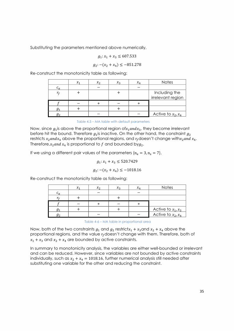
Substituting the parameters mentioned above numerically,

Re-construct the monotonicity table as following:

Notes Including the

irrelevant region + + Active to

Now, since is above the proportional region of , they become irrelevant before hit the bound. Therefore is inactive. On the other hand, the constraint restricts above the proportional regions, and doesn’t change with . Therefore, is proportional to and bounded by .

If we using a different pair values of the parameters ( ),

Re-construct the monotonicity table as following:

Notes + + Active to Active to

Now, both of the two constraints and restrict and above the proportional regions, and the value doesn’t change with them. Therefore, both of

and are bounded by active constraints.

In summary to monotonicity analysis, the variables are either well-bounded or irrelevant and can be reduced. However, since variables are not bounded by active constraints individually, such as , further numerical analysis still needed after substituting one variable for the other and reducing the constraint.

Table 4-6 – MA table in proportional area

Table 4.5 – MA table with default parameters

36

4.5 Numerical Results

The problem is formulated as following:

Subject to:

Using function ga in MATLAB with parameters in the values mentioned above, the result shows as following:

Design variables or dependent variables values ws (x1) 496.461 ls (x2) 561.6384

wb (x3) 105 lg (x4) 289.6384

wa 341.234 re 36 ca 216 rf 1 g1 601.461 (inactive) g2 851.278 (active) f* -216

The result consists with the monotonicity analysis. The constraint is inactive but is active. In addition, since are irrelevant and doesn’t change with , which are bounded by and beyond the proportional region, remains 1 and the objective, , only depends on , which is bounded by . Therefore, the optimum value is boundary optimum.

Table 4.7 – Numerical result with default parameters

37

4.6 parameter study

If changing the parameters, , with different values, the results are shown as below:

ne 3 3 4 4 5 5 ns 6 7 6 7 6 7

ws (x1) 496.461 415.7429 481.1057 415.7429 423.9654 386.4701 ls (x2) 561.6384 660.2777 470.0424 492.8849 560.8905 530.6563

wb (x3) 105 105 117.9823 105 182.5689 133.8977 lg (x4) 289.6384 357.8787 244.9097 220.8849 128 216.9052

wa 341.234 304.7997 355.472 304.7997 310.7942 307.4254 re 36 36 30.625 36 25 29.7 ca 216 216 245 288 250 297 rf 1 0.8658 0.9921 0.8658 0.9928 0.8658 g1 601.461 Active 599.088 Active 606.5343 Active g2 Active Active -714.952 -713.77 -688.891 -747.562 f* -216 -187 -244 -249 -248 -258

From the chart above,

A larger makes to be active, and then shrinks the value of . Therefore, no matter what the capacity ( ) is, there is a discount on it.

A smaller makes to be active, and then bounds the value of , which means that the number of exits restricts total capacity of the plane in small number. When the number becomes larger, it becomes less critical.

The optimum value occurs in the case of =5, and =7. The reason is that even thought there is a discount because of small seat, it has the largest capacity ( ) to maximize the number of passenger.

In summary, the problem is bounded and local minimum for each case exists. However, without changing parameters, the result of optimization is less obvious since the problem involves several discrete results and the objective function varies with design variables only in limited regions. If taking the parameters as discrete variables or adding more deign freedom, the optimization might be more significant.

Table 4.8 – Numerical result with parametric study

38

4.7 Discussion

In this subsystem study, we found the relations between passengers on broad and the dimensions of the plane and the seat. According to the result under current number of exists and seat per row, the total number of seats is restricted by the regulation on emergence exists. According to the present A320 data, the max capacity, for only one class operation, is 180 seats, which satisfies the constraint and is below the optimum value, 216 seats. Consequently, there are still some rooms for improvement under the current parameters.

Even more, the maximum capacity can also be induced by inducing more emergency exits and the seats in each row. As shown in the result of parameter study, the value of seats can be maximized up to 258. But if setting more seats with smaller size, the width will not be as suitable as the larger ones for passengers and shrinks the fitness rate. Therefore, airline companies should design as many as exists as possible, whereas the target passengers’ body size should be considered before increasing the number of seat on each row. The companies might adjust the design for different target customers in different operation areas.

Due to the difficulty of public survey on different chair configuration, this study didn’t consider passengers’ comfort, which will be a more reasonable factor reflecting the passengers’ willingness than fitness. For future study, with enough period time and tools, this factor should be taken into consideration. However, this study provides the linking from dimension of a plane to the maximum possible number of passengers. It ought to be a good tool to predict the efficiency in plane design.

4.8 Reference

[1] M Kaufmann, D Zenkert and P Wennhage, 2009, “Integrated cost/weight

optimization of aircraft structure,” Struct. Mutltidiscip. Opt. 41(2) pp325-334.

[2] G Nadadur and M Parkinson “Using Designing for Human Variability to Optimize Aircraft Seat”

[3] e-CFR (electronic Code of Federal Regulation) Data of Feb. 10, 2011, Title14: Aeronautics and Space

[4] NTSB (The Regulations on Flight Attendant Exit Assignment), tel. 202/314-6219 [5] Airbus group website

39

5 Subsystem – Turbofan Engine (Chun-Shiang Lin)

5.1 Problem Statement

The engine is the source for propulsion. Higher power output leads to faster travel

and higher allowable capacity, but fuel consumption is compromised. However, higher

power output usually leads to heavier and larger engine size, which also compromises fuel

consumption.

The design objective will be minimizing the specific fuel consumption under certain

settings and parameters. This work deals specifically with thermodynamic cycle design. The

process consists of calculations based on thermodynamic changes that the air and gases

pass through the engine components. Traditionally, the cycle design involves numerous

parametric variations, and it becomes more difficult when the design constraints are

introduced. The way simplify the problem is to select design ratio variable instead of

choosing certain single value variables. And finally make comparison to airliner A 320

Engine. The current engine efficiency is listed below:

Type Thrust

(kN)

Bypass

ratio

Compression

ratio

Fan

diameter

(m)

Total

length

(m)

Weight

(kg)

Production

start year

aircraft

type

V2500 111 5.4:1 35.8:1 1.587 3.2 2,387 1989 A320

Table 5.1 A320 engine design

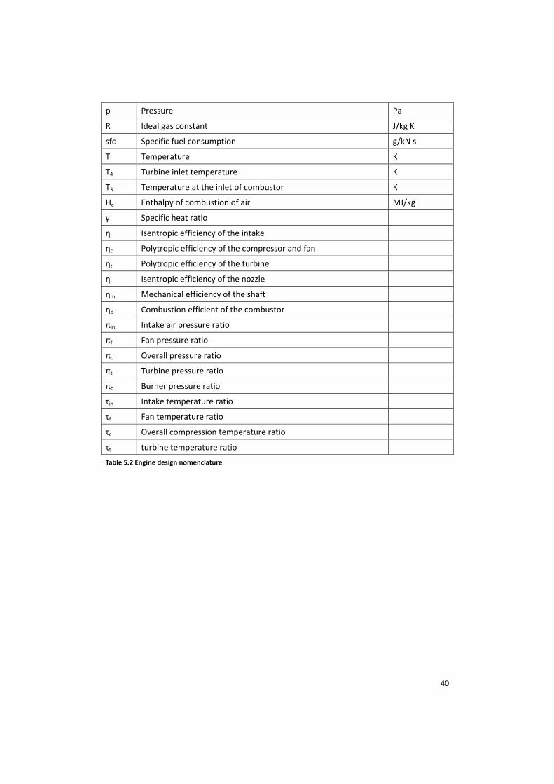
5.2 Nomenclature

symbol meaning unit

A Area m2

As Specific area (area/unit mass flow rate) m2 s/kg

B Bypass ratio =

Ca Velocity magnitude of air m/s

Cp Constant pressure specific heat J/kg.K.

D Diameter of fan m

F Thrust N

Fs Specific thrust (thurst/total air mass flow rate Ns//Kg

f Fuel air ratio of core flow (mass flow rate of fuel /mass flow rate

of core air flow)

mh Air mass flow rate at the core Kg/s

mc Air mass flow rate bypass the core Kg/s

ma Total air mass flow rate at the core Kg/s

40

p Pressure Pa

R Ideal gas constant J/kg K

sfc Specific fuel consumption g/kN s

T Temperature K

T4 Turbine inlet temperature K

T3 Temperature at the inlet of combustor K

Hc Enthalpy of combustion of air MJ/kg

Specific heat ratio

i Isentropic efficiency of the intake

c Polytropic efficiency of the compressor and fan

t Polytropic efficiency of the turbine

j Isentropic efficiency of the nozzle

m Mechanical efficiency of the shaft

b Combustion efficient of the combustor

in Intake air pressure ratio

f Fan pressure ratio

c Overall pressure ratio

t Turbine pressure ratio

b Burner pressure ratio

in Intake temperature ratio

f Fan temperature ratio

c Overall compression temperature ratio

t turbine temperature ratio

Table 5.2 Engine design nomenclature

41

5.3 Mathematical Model

5.3.1 Objective function

To find the effect of combination of four cycle design variables that minimizes the

specific fuel consumption. The thrust produced by the engine is the sum of momentum and

the pressure difference . The velocity in the formula could further be expressed in

temperature difference by using thermo energy equilibrium. A schematic diagram of

turbofan engine is shown in figure 1.

1 2 3 4 5 6 8 7

Figure 5.1 Engine schematic diagram

Objective function:

Specific fuel consumption (SFC) =

Where Fs= =

f :mH CPA(T3 298.15) +f mH b HC=( mH+f mA) CPG (T4 298.15)

now try to find the expression for C7 ,C8 , P7 ,P8 , , in terms of input variables.starting

with the core nozzle , the definition of stagnation temperature gives:

CPG T07= CPGT7+ C72 /2

C7=(2CPG(T07 T7))0.5=(2CPG(T06 T7))0.5

An expression for T06 is found by making energy balance over the gas generator on a unit

basis:

mc

mh

compressor TurbineCombustor

42

(1+f) CPG (T04 T06)= (T02 T01)+ (T03 T01) (1)

T04 T06= T01[B( 1) +( 1)

And making the following definitions:

in , in=

f , in=

c , c=

t , t=

f= f(n 1)/n ,

c= c(n 1)/n

in= 1+

j=

Combined all the definitions above and energy equation(1) we will get the expreseeion for

T7=T04 t{ 1 j[1 ( ) rg 1/rg ]}

Assuming nozzle is unchecked then we are able to yield :

C7={ 2 CPG T04 t j[ 1( ) rg 1/rg ]}0.5

The density of exaust gas is given by :

7=

then we can yield the specific area As7:

As7 = =

Similarly , for the bypass nozzle we can derive from the energy equation and yield similarly

expressions , the definition of stagnation temperature gives:

CPG T08= CPGT8+ C82 /2

C8=(2CPG(T08 T8))0.5=(2CPG(T02 T8))0.5

Also assume nozzle is unchoked in here:

T8=Ta in f{ 1 j[1 ( ) rg 1/rg ]}

43

C8={ 2 CPa Ta in f j[ 1( ( ) rg 1/rg ]}0.5

Now we have expressions for C7 ,C8 , P7 ,P8 , , and f in terms of four variables bypass

ratio B , fan pressure f , overall air pressure c and inlet turbine temperature T04.

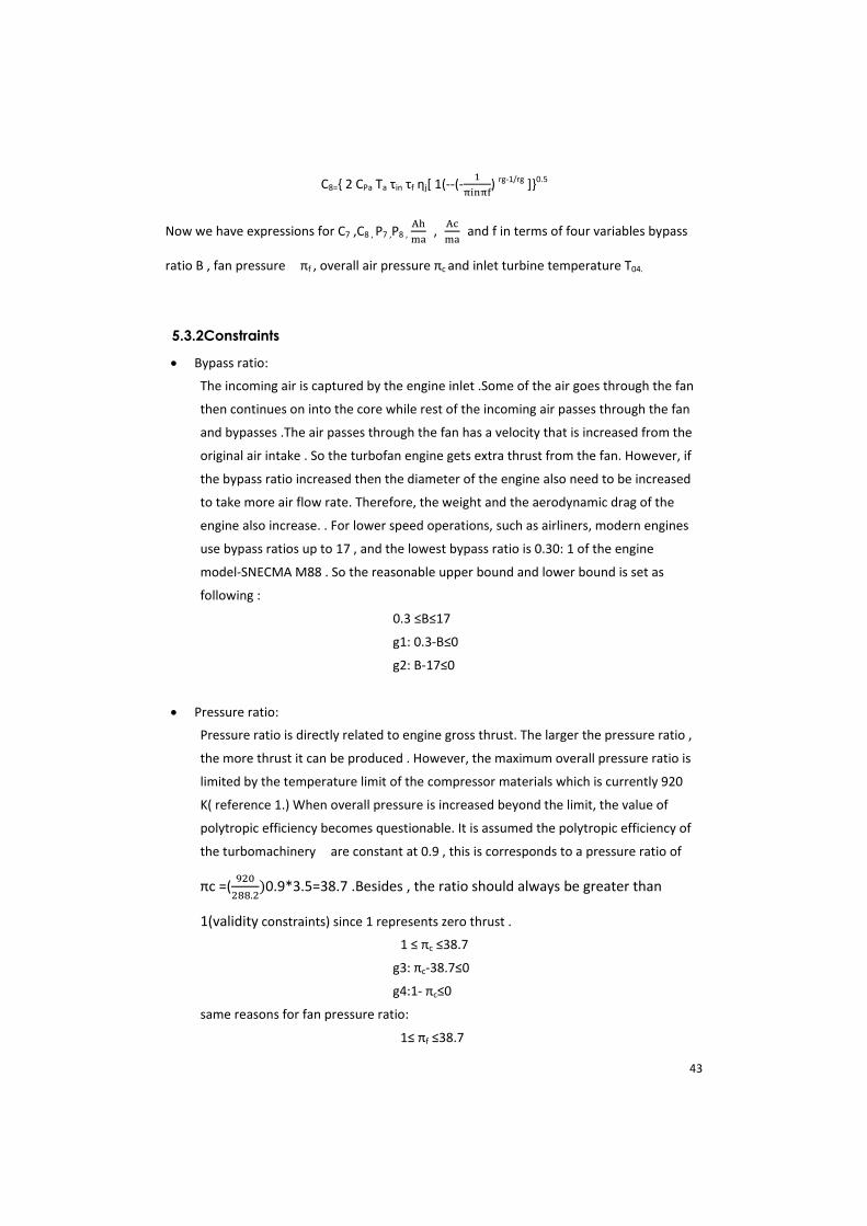
5.3.2Constraints

Bypass ratio:

The incoming air is captured by the engine inlet .Some of the air goes through the fan

then continues on into the core while rest of the incoming air passes through the fan

and bypasses .The air passes through the fan has a velocity that is increased from the

original air intake . So the turbofan engine gets extra thrust from the fan. However, if

the bypass ratio increased then the diameter of the engine also need to be increased

to take more air flow rate. Therefore, the weight and the aerodynamic drag of the

engine also increase. . For lower speed operations, such as airliners, modern engines

use bypass ratios up to 17 , and the lowest bypass ratio is 0.30: 1 of the engine

model SNECMA M88 . So the reasonable upper bound and lower bound is set as

following :

0.3 B 17

g1: 0.3 B 0

g2: B 17 0

Pressure ratio:

Pressure ratio is directly related to engine gross thrust. The larger the pressure ratio ,

the more thrust it can be produced . However, the maximum overall pressure ratio is

limited by the temperature limit of the compressor materials which is currently 920

K( reference 1.) When overall pressure is increased beyond the limit, the value of

polytropic efficiency becomes questionable. It is assumed the polytropic efficiency of

the turbomachinery are constant at 0.9 , this is corresponds to a pressure ratio of

c =( 0.9*3.5=38.7 .Besides , the ratio should always be greater than

1(validity constraints) since 1 represents zero thrust .1 c 38.7

g3: c 38.7 0

g4:1 c 0

same reasons for fan pressure ratio:

1 f 38.7

44

g5: f 38.7 0

g6:2 f 0

Also the overall pressure is larger than fan pressure ratio :

g7: f c 0

Thrust to weight ratio : As we choose the certain model of airliner , the thrust have to

be larger than the minimum thrust based on the thrust to weight ratio .For

propeller driven aircraft, the thrust to weight ratio can be calculated as follows

where is propulsive efficiency at true airspeed V P is engine power. In

order for the plane to take off the ground , the thrust �–to Weight ratio need to be

larger than 1(validity constraints). Take A 320 engine model for the case :

1 , F 2387 Kg*m/s2

g8: 2387 Fs*Ca* D2/2 0

Inlet turbine temperature: A smaller core airflow needs to be large enough to provide

sufficient power to drive the fan and compressor. The larger temperature difference

could convert more work output for shaft work. The tolerable temperature limit is set by

the turbine blades— usually the first stage. Modern turbine blades are single metal

crystals with hollow interiors. Cooler air from the compressor is blown through the hollow

interior of the blades. Normally the melting temperature of the blade material (around 1600

°C).

g9: T04 1600 °C

In order to produce enough thrust which is being positive value of the function , C7 ,C8 ,P7 ,P8 has to be larger than Ca , Pa first we take the condition under flying at 9000 feet

hight , mach number =0.8 , Ca=264.95 m/s , Pa=72.40 kpa

g10:264.95- C7 0g11:264.95- C8 0g12:72.40kpa P7 0g13: 72.40kpa �– P8 0

5.3.3 Design Variables and Parameters

Design variables: Typical range

1. Bypass ratio B 0.3 B 172 Fan pressure ratio f 1 F 38.73 Overall pressure ratio c 1 c 38.74 Turbine inlet temperature T04 T04 1600 °C

45

Table 5.3 Design variables and typical value

In here I take the kerosene as fuel for AE 320 engine model , all the properties of fluids ,

performance parameters and operating conditions are listed below:

Parameters: Default value

Altitude 9000feet

Mach number 0.8

Weight 2387 kg

Air temperature 272.516 K

P air pressure 72.40 kpa

CPa (constant specific heat for air) 1.0035 kJ/g *k

cpg (constant specific heat for gas) 2 kj/g*k

Hc 77.8 KJ/Kg

Ta 272.516 k

i 0.9

c 0.8

b 0.8

m 0.8

t 0.9

j 0.9

t 0.8

in 1

t 0.4579

in 1

Ra 0.287 KJ/kg K

Rg 0.189 KJ/kg K

A 1.2920 kg/m3

g 817.15 kg/m3

H 43.1 Mj/kg

D 1.587 m

Table 5.4 Parameter value

5.3.4 Summary Model

The model aims to minimize the function of SFC with four design variables

Min SFC =

Where ,

46

Fs= =

C7={ 2 CPG T04 t j[ 1( ) rg 1/rg ]}0.5

C8={ 2 CPa Ta in f j[ 1( ( ) rg 1/rg ]}0.5

= 7 RgT7= 7 Rg T04 t{ 1 j[1 ( ) rg 1/rg ]}

= 8 RaT8= 8 Rg Ta in f{ 1 j[1 ( ) rg 1/rg ]}

f :mH CPA(T3 298.15) +f mH b HC=( mH+f mA) CPG (T4 298.15)

subject to,g1: 0.3 B 0g2: B 17 0g3: c 38.7 0g4:1 c 0g5: f 38.7 0g6:1 f 0g7: f c 0

g8: 2387 Fs*Ca* D2/2 0g9: T04 1600 °C g10:264.95- C7 0g11:264.95- C8 0g12:72.40kpa P7 0g13: 72.40kpa �– P8 0

where,

C7={ 2 CPG T04 t j[ 1( ) rg 1/rg ]}0.5

C8={ 2 CPa Ta in f j[ 1( ( ) rg 1/rg ]}0.5

T7=T04 t{ 1 j[1 ( ) rg 1/rg ]}

T8=Ta in f{ 1 j[1 ( ) rg 1/rg ]}

5.4 Model Analysis

5.4.1 Monotonicity Analysis and Well-Boundedness

47

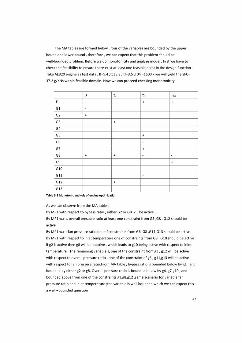
The MA tables are formed below , four of the variables are bounded by the upper

bound and lower bound , therefore , we can expect that this problem should be

well bounded problem. Before we do monotonicity and analyze model , first we have to

check the feasibility to ensure there exist at least one feasible point in the design function .

Take AE320 engine as test data , B=5.4 , c35.8 , f=3.5 ,T04 =1600 k we will yield the SFC=

37.2 g/KNs within feasible domain. Now we can proceed checking monotonicity.

B c f T04F + +

G1

G2 +

G3 +

G4

G5 +

G6

G7 +

G8 + +

G9 +

G10

G11

G12 +

G13

Table 5.5 Monotonic analysis of engine optimization

As we can observe from the MA table :

By MP1 with respect to bypass ratio , either G2 or G8 will be active ,

By MP1 w.r.t. overall pressure ratio at least one constraint from G3 ,G8 , G12 should be

active

By MP1 w.r.t fan pressure ratio one of constraints from G6 ,G8 ,G11,G13 should be active

By MP1 with respect to inlet temperature one of constraints from G8 , G10 should be active

if g2 is active then g8 will be inactive , which leads to g10 being active with respect to inlet

temperature . The remaining variable s, one of the constraint from g3 , g12 will be active

with respect to overall pressure ratio . one of the constraint of g6 , g11,g13 will be active

with respect to fan pressure ratio.From MA table , bypass ratio is bounded below by g1 , and

bounded by either g2 or g8. Overall pressure ratio is bounded below by g4, g7,g10 , and

bounded above from one of the constraints g3,g8,g12 .same scenario for variable fan

pressure ratio and inlet temperature ;the variable is well bounded which we can expect this

a well �–bounded question

48

5.5 Numerical Results

5.5.1 Model Robustness and Global Minimum

The function genetic algorithms (GA) and fmincon were used to minimize the following

objective function:

Min SFC =

The initials points were picked from the feasible region , below chart is the resultsfrom different starting point :

X0( B , f , c,, T04) SFC(GA) SFC(fmincon)

(10 , 5, 30 , 1000) 59.0206 g/kN s 55.3356 g/kN s( 5 ,5 , 20 , 1000) 59.0208 g/KN s 55.3355 g/kN s(10 , 10 ,30,500) 59.0205 g/KN s 55.3356 g/kN s( 2 , 5 , 20 , 1500) 59.0203 g/KN s 55.3354 g/kN s(5 , 15 , 10 , 1500) 59.0208 g/KN s 55.3355 g/kN s

Table 5.6 Numerical results from fmincon and GA

From the chart above , I chose the sfc output up to four significant digits .We can

observe the results are the same with different settings of initial points . All initial points

leads to the same Xopt =(1.5599 ,2.0015 , 34.8561 ,1.6323e+3) . Plus, based on report, g8 is

active which is consistent with the monotonicity analysis. Supposedly, substitute g8 into

objective function will eliminate one of the variable and the function becomes three degrees

of freedom problem. The results of this objective function should be the same since it is

interior optimal point. However, many parameters involve in objective function so that this

is hard to guarantee g8 will stay active all as I change my parameters value. Therefore, I

don�’t simplify my objective function by eliminating one of the variables when I do

parametric study. Moreover, the reasonable approach to evaluate the constraint activity is

by checking the value of lagrangian multipliers.

1 0 6 0 11 02 0 7 0 12 03 0 8 0.735 13 04 0 9 05 0 10 0

Table 5.7 Value of lagrangian multipliers for engine design constraints

All the multipliers are zero except G8. In other words, mutiplier 8 >0 that satisfiesthe KKT regular point condition and g8 is the only active constraint. When fmincon

was used to compare the results of GA algorithm, optimization of sfc values are slightly

49

different. This result is largely due to iteration limits of fmincon and generation numbers

&population size were not set large enough, if these two algorithm set the iteration large

enough then we will yield similar results. The results suggest that the bypass ratio shouldn�’t

be too large, and the larger overall pressure ratio the better, yet the fan pressure will be

best designed for slightly larger than twice the air compress ratio.

5.5.2 Model Parametric Studies

Ideally, the parameters treat as variable in other subsystems should bepriority choice to do parametric studies. As we are able to see in other systems,cabin size, length and width will have a significant effect on thrust to weightratio constraint. Therefore, changing the value of weight will be chosen as firstparametric study.

Case Weight(kg) B f c T04 SFC

1 900 16.9989 4.6783 28.8450 1.3292e+3 35.4783

2 1100 16.9890 4.3275 29.7049 1.3762e+3 43.928

3 1300 15.7934 3.9257 30.2594 1.4203e+3 46.3019

4 1500 13.5284 3.6920 31.4802 1.4895e+3 49.271

5 1700 9.2548 3.2192 31.6305 1.5334e+3 51.2470

6 1900 7.3702 2.7489 32.3403 1.5563e+3 52.3792

7 2100 3.4784 2.4784 32.7851 1.5644e+3 54.2389

8 2300 1.4782 2.1125 34.1003 1.6202e+3 58.0654

9 2500 1.4573 1.9647 34.7964 1648.2e+3 64.8034

10 2700 1.3790 1.4954 34.9009 1680.8e+3 66.7206

11 2900 1.2397 1.3428 35.1758 1689.5e+3 70.3892 Table 5.8 Parametric study under different weight

One outstanding feature we can observe from the chart is that bypass ratio

becomes limiting factor once weight load drops at certain value. This means that

at low weight to thrust ratio, the objective function becomes three dimensional

problem. Furthermore, we are able to see that sfc decreases when weight is

increased. We can expect the weight will have tremendous effect when we try to

put up all the subsystems. While weight play major role in constraint function,

50

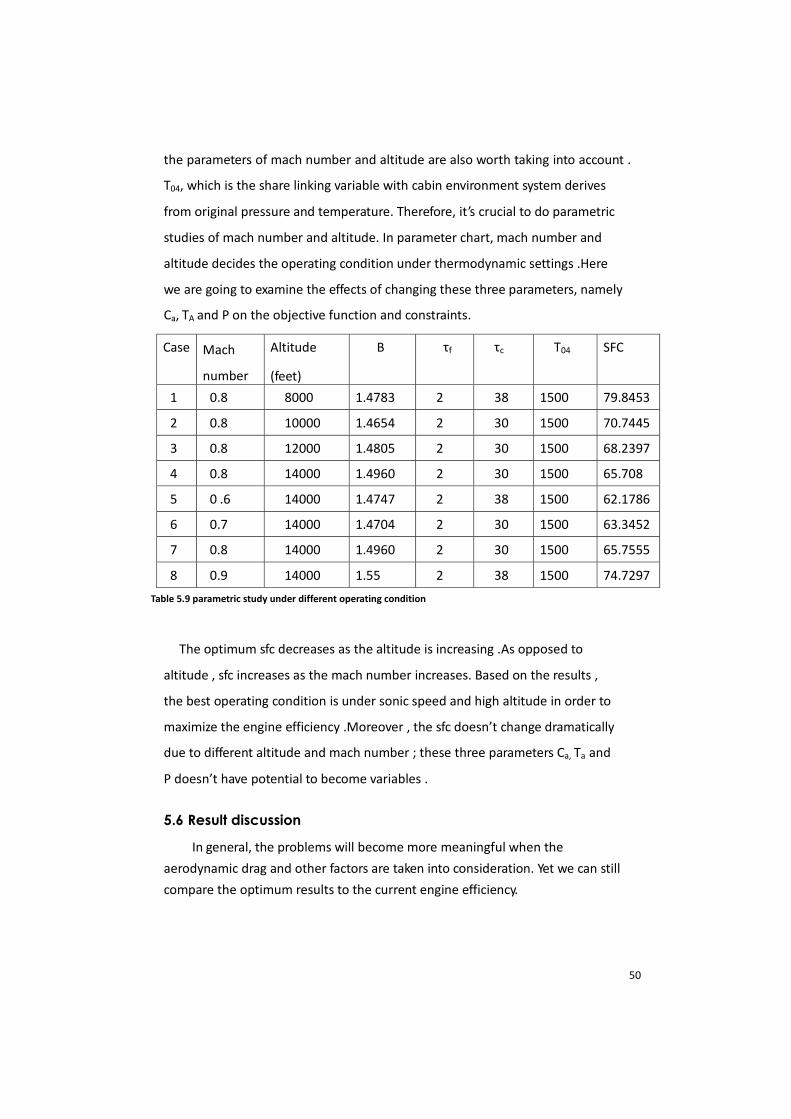
the parameters of mach number and altitude are also worth taking into account .

T04, which is the share linking variable with cabin environment system derives

from original pressure and temperature. Therefore, it�’s crucial to do parametric

studies of mach number and altitude. In parameter chart, mach number and

altitude decides the operating condition under thermodynamic settings .Here

we are going to examine the effects of changing these three parameters, namely

Ca, TA and P on the objective function and constraints.

Case Mach

number

Altitude

(feet)

B f c T04 SFC

1 0.8 8000 1.4783 2 38 1500 79.8453

2 0.8 10000 1.4654 2 30 1500 70.7445

3 0.8 12000 1.4805 2 30 1500 68.2397

4 0.8 14000 1.4960 2 30 1500 65.708

5 0 .6 14000 1.4747 2 38 1500 62.1786

6 0.7 14000 1.4704 2 30 1500 63.3452

7 0.8 14000 1.4960 2 30 1500 65.7555

8 0.9 14000 1.55 2 38 1500 74.7297 Table 5.9 parametric study under different operating condition

The optimum sfc decreases as the altitude is increasing .As opposed to

altitude , sfc increases as the mach number increases. Based on the results ,

the best operating condition is under sonic speed and high altitude in order to

maximize the engine efficiency .Moreover , the sfc doesn�’t change dramatically

due to different altitude and mach number ; these three parameters Ca, Ta and

P doesn�’t have potential to become variables .

5.6 Result discussion

In general, the problems will become more meaningful when theaerodynamic drag and other factors are taken into consideration. Yet we can stillcompare the optimum results to the current engine efficiency.

51

Type Thrust

(kN) Bypass

ratio

Compression

ratio

Fan

diameter

T04 Weight

(kg) aircraft

type

V2500 111 5.4:1 35.8:1 1.587 1205K 2,387 A320Optimum 343 1.5599:1 34.8561:1 1.587 1632K 2,387

Table 5.10 Engine results comparison

The overall compression ratio is about the same, but there�’s a significant

difference as opposed to bypass ratio. While it is true that the sfc calculated

from cycle analysis appears to improve continuously as bypass ratio is increased,

this doesn�’t hold true when installation effects are accounted for. In this case,

the current design requires larger engine size to overcome the drag, which is not

much fuel efficiency to be gained when bypass ratio is larger than certain value.

Better thermal withstand material results in higher inlet temperature in

optimal design. As it is mentioned at earlier section, higher inlet temperature will

lead to higher engine efficiency. However, the materials used for turbine blade

can�’t withstand this high temperature. If we are able to improve the material

property, we will yield higher engine efficiency.

5.7 Reference

[1] Effects of Fuel Consumption of Commercial Turbofans on Global Warming

Onder Turan and T. Hikmet Karakoc

[2] Kapadi, Yogesh; Pashilkar, Abhay

Aero thermodynamic model for digital simulation of turbofan engine

Yadav, R. (Department of Mechanical Engineering, Motilal Nehru National

institute of Technology, Allahabad 211004, India

52

6 All-in-One System

6.1 Problem Statement

In this chapter, we return to the problem of profit maximization and combine the four

above-mentioned subsystems into an overall system. The profit of an aircraft can be

calculated via its income and its expense. However, lots of factors would influence

these two, such as the concurrent fuel price, the number of passengers, and the

efficiency of jet engines, the reputation of an airline company, and etc. As we can see,

these complexity issues cannot be modeled completely. In this study, we ignore the

non-engineering related cost, such as administrative cost for pilots and stewards.

For different operational situations, the cost value would be different. For the

reasonable simplification in this AIO system, we only take the following two factors into

account, the income from the quantity of tickets sold and the cost from expenditure of

fuel. For the income part, the amount of tickets sold can be maximized by through the

process described in the seat arrangement subsystem. By picking a specific journey,

and using the current ticket price, we can calculate the income gained by using the

craft. For the cost part, the fuel consumed can be estimated by multiplying the specific

fuel consumption (SFC), which presents the mount of gasoline needed per thrust, with

extra engine load and the price of gasoline as well as duration of the flight. The price of

gasoline and the flight time can be set as a parameter here.

Therefore, by the relationship mentioned above, the connections between overall profit

results of each subsystem are established, and can be formulated as following.

= # $ $

For maximizing the profit, it’s obvious to maximize the number of passengers and to

minimize both of SFC and extra engine load.

53

6.2 Nomenclature

Design Variable Definition Unit

Environment Control System (CAU) Compressor Inlet

temperature ( C)

Compressor outlet temperature

( C)

Compressor Inlet pressure (kPa)

Mass of refrigerant (kg)

Fuselage Structure (FSU)

wt Web thickness Meter

p Pitch between beams Meter

fw Flange width Meter

ftt Flange thickness Meter

ftb Flange thickness Meter

st Shell thickness Meter

Seat Arrangement (SA)

Ws seat width (mm)

Wb Distance between seats, Arm room

(mm)

Ls seat length (mm)

Lg lag room (mm)

Turbofan Engine (TFE)

B Bypass ratio

Fan pressure ratio

Overall pressure ratio

T04 Turbine inlet temperature (K)

Linking Variables

Lc Cabin length (m)

Wc Cabin width (m)

T04 Turbine inlet temperature (K)

Table 6.1 – Nomenclature for the AIO system. Both linking and local variables are shown

54

For a complete list of AIO system parameter nomenclatures refer to Appx-A.

6.3 Mathematical Model

6.3.1 Objective Function

The profit functional relation to different subsystem outputs is shown in the equation

above. To summarize the optimization problem we have the following.

min       = (# $ $ )

Where,

= ( , )

The TFE function is the turbofan engine subsystem with the combined weight of all other

three subsystems and increased fuel consumption (IFC) as input. The combined weight

will serve as the constraint lower bound for the TFE function and the IFC will add the

extra required fuel in the TFE function. IFC is an output from the CAU subsystem as

described in the CAU section.

The Fload the extra required load by the engine to carry the extra weight. We first looked

up nominal thrust (120 kN) of the A320 aircraft and the nominal empty aircraft weight

(42600 kg). Then with the extra weight due to the three subsystems we can find the

extra lift required by the aircraft to fly at the same conditions, such as speed and climb

rate. Fixing the same wing geometry and varying slightly the flap configurations we can

increase the coefficient of lift. With increased coefficient of lift, there is also an

increased coefficient of induced drag. Coefficient of induced drag is proportional to

increased coefficient of lift squared. Then the required thrust must equate to the new

increased drag and we find the following function as the relationship for the Fload.

= 120000 × (1 + 42600 × )

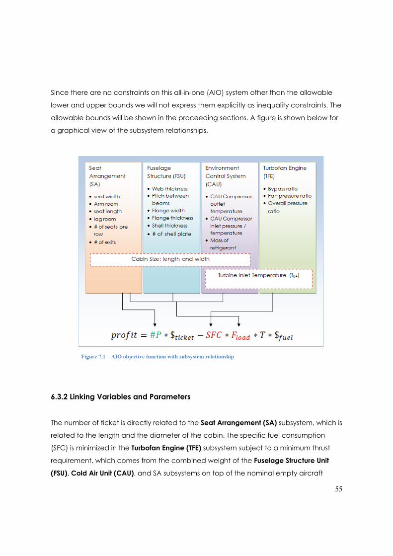
55

Since there are no constraints on this all-in-one (AIO) system other than the allowable

lower and upper bounds we will not express them explicitly as inequality constraints. The

allowable bounds will be shown in the proceeding sections. A figure is shown below for

a graphical view of the subsystem relationships.

6.3.2 Linking Variables and Parameters

The number of ticket is directly related to the Seat Arrangement (SA) subsystem, which is

related to the length and the diameter of the cabin. The specific fuel consumption

(SFC) is minimized in the Turbofan Engine (TFE) subsystem subject to a minimum thrust

requirement, which comes from the combined weight of the Fuselage Structure Unit

(FSU), Cold Air Unit (CAU), and SA subsystems on top of the nominal empty aircraft

Figure 7.1 – AIO objective function with subsystem relationship

56

weight. The engine turbine inlet temperature (T04) is related to the CAU subsystem. The

engine load is defined as the combined SA, CAU, and FSU weight on top of the nominal

empty aircraft weight. There are also increased fuel consumption due to the operation

of the CAU compressor and air bleeding in the turbofan compressor. The increased fuel

consumption is also linked to the SFC.

Higher T04 provides higher available thrust for the turbofan engine but also requires

higher cooling capacity from the CAU as the temperature difference with respect to

the room condition increases. These subsystems show a conflict of interest and optimal

target direction.

Larger cabin dimensions, namely the cabin length and the diameter affect the SA, FSU,

and CAU subsystem. With a larger value of length and diameter, more passenger

capacity is allowed but higher volume of air is needed to be cooled by the CAU. So this

increases the number of ticket sales but also increases the required CAU compressor

work and possibly the refrigerant mass. Larger cabin diameter and length also affect

the structural stiffness of the FSU subsystem. Longer cabin will require higher bending

stiffness which will require a larger bending inertial that may ultimately increase the

overall structural weight. Contrarily, a larger cabin diameter increases the bending

inertia pushing the overall structural mass to the circumference increasing the bending

stiffness and decreasing the weight, but buckling strength is compromised.

To summarize, the following shows the linking variables among the four subsystems and

their allowable bounds.

Linking Variable Definition Allowable Range

Lc Cabin Length (m) [30, 50]

Wc Cabin Width (m) [3.5, 4.2]

T04 Turbine Inlet Temperature (K) [700, 1873]

Table 6.2 – List AIO linking variables with allowable upper and lower bounds

57

As mentioned above, the AIO objective function includes four parameters. The

parameters and the chosen value are summarized below.

Parameter Definition Typical Value

Wavg_p Average Passenger Weight (kg) 80

$ticket Ticket Price (USD) 200

$fuel Fuel Price (USD/kg) 1

tflight Flight Time (s) 18000

The average weight for the world population was estimated to be about 80 kg. The

domestic ticket price was taken over the average price from a number of airline

websites for 5 hours domestic flights. The price was determined to be around $200. The

fuel price was taken from online sources with the current Jp-8 fuel price.

Table 6.3 – List AIO parameters with the selected values

58

6.4 AIO Model Integration

Since all of the optimization work for each of the subsystems were done with Matlab

function fmincon, it is most convenient to integrate the subsystems with Matlab and

fmincon. The following shows a map of the subsystem function integration loop.

An overall fmincon function is applied to the AIO objective function with the linking

variables. The AIO objective function then calls each of the individual subsystem

objective functions passing in the linking variables to each. Since most of the linking

variables were originally set as parameters in the subsystem studies, the new

Figure 6.2 – System integration flow chart

59

parameters will now be redefined every outer iteration step. The subsystem objective

functions are also modified to separate the output into the desired variables. The

weighs for subsystems CAU, FSU, and SA will be passed into the TFE subsystem for the

thrust constraint. Separately, the CAU will also pass IFC into the TFE subsystem for the

increased fuel consumption. The TFE subsystem will then combine the outputs from the

other three subsystems and output the final SFC into the AIO objective function loop.

The SA subsystem will also output the #passenger into the outer loop. The process then

reiterates until the optimum is reached.

6.5 Result Analysis

6.5.1 Numerical Results

Lc Wc T04 Revenue

31.11m 4.1m 1694 13848

CAU

(subsystem

weight)

FSU (subsystem

weight)

SA (subsystem

capacity)

TFE (SFC)

AIO 1300 kg 1266 kg 137 passengers 7.32E-6 kg/N-s

Individual 1034 kg 1330 kg 216 passengers 55.3E-6kg/N-s

6.5.2 Global Convergence Study

In all-in-one system, proving the system’s convergent status is fairly important.

Starting points are selected based on the variable’s upper bound and lower

bound. Here we choose zero represents lower bound while 1 represents upper

bound. Since we have three linking variables in overall system, eight sets of

starting points are chosen to test robustness of the system.

Table 6.4 – List AIO optimizers and objective function value

Table 6.5 – List subsystem output with AIO and individual optimization

60

Lc (m) Wc (m) T04 (K) Fval [0 1 0] 30 3.97 1873 -2.54*104

[1 0 0] 31.10 4.07 1693 -2.67*104 [0 0 1] 30 4.2 1873 -2.54*104 [0 0 0] 43.74 3.81 1693 -2.67*104 [1 1 0] 30 4.15 1694 -2.69*104 [1 1 1] 50 4.2 1873 -2.53*104 [1 0 0] 30 4.2 1414 -2.68*104 [1 0 1] 30 3.91 1873 -2.54*104

Table above shows the average of final value of -2.56*104 and the largest

margin is 5%. Therefore, no matter how we choose starting points in feasible

region, the results will converge within ±5% of average final value. Therefore in a

sense, we can call this a global minimum with an uncertainty of ±5%. Since we

employed a relatively crude profit model for the AIO system, our optimal

function value merely shows a relative profit figure instead of an absolute one. In

airline industry, the predictable revenue and performance of each airline is

crucial for complex economy management. Giving the flexibility of diameter,

length, and different operating condition to choose from in airline design, mass

customization will meet the customer’s need in this competitive market.

6.5.3 Parametric Study

By examining our proposed profit model, the parameters are price of ticket and fuel.

The variations from parameters represent how earning and cost influence on the profit

model. If the fuel price is much cheaper than the default value, it is reasonable for a

company to earn more money by carrying more passengers with slightly increasing in

the fuel cost, and vice versa. Therefore, the parametric study is required to understand

how the ticket and fuel price affect the objective model and the design variables.

Since the parameters in the objective model are linear to the design variables, they

Table 6.6 – List various starting points and the optimal AIO function value.

61

should not be simultaneously increased at the same rate; otherwise, the result is

expected as linear. Therefore, we only change the price of ticket from 20 to 1000 and

fix the price of oil at the mean while. The result is as the following table.

Ticket Price ( $USD) 20 100 500 1000 Cabin Length (m) 30 30 30 30 Cabin Width(m) 3.62 3.54 3.53 3.67

Inlet Temperature (K) 1693 1693 1693 1693 Revenue 2276.5 13128 67380 135200

The result indicates that our profit model is highly linear. However, the cabin length does

not elongate as expected as the increase of ticket price. By examining the subsystem,

we found that the structure model would prevent the increase of cabin length due to

the violation of bending moment constraint. In addition, the longer the cabin is the

more weight the system obtains. Moreover, in such condition, the cold air unit would

require more refrigerant to meet the design requirement and hence increase the

weight as well. The increase of weight would directly deteriorate the SFC factor and

raise the operation cost. Hence the ticket price does not affect the model as

expected.

6.5.4 Result Discussion and Interpretation

The result in the all-in-one problem differs from the outcome of each subsystem. Two of

the subsystems, namely, Seat Arrangement and Cold Air Unit performance are inferior

to the previous optimization. On the other hand, the Fuselage structure and Turbofan

Engine have better performance. Under the linking variables we chose for overall

system, fuselage structure and turbofan engine play more important role in maximizing

the profit. The result of linking variables can be interrelated as the following.

Based on the proposed profit model, the number of passengers is proportional to the

income. The larger the cabin size, the more people will be able to fit in an aircraft.

However with increased passenger capacity, the overall weight increases significantly

Table 6.7 – Parametric study results

62

as well. From the numerical results, we see the SA subsystem comprises of more than

76% of the total weight of the three subsystems. Therefore the SA subsystem objective

function plays an important role in both the earnings and the cost. Table(*) shows that

length of the cabin shortens to 31.11 meters compared with the original model A320,

which means the capacity for passengers is significantly reduced, which means that

the fuel cost effect dominates the earnings per passenger once the capacity reaches

137. There is a minimum point for the number of passengers. The cost is also decreased

due to light weight of fuselage structure and lower engine load. Comparing the trade-

off between these two further shows that lighter weight dominates passenger capacity.

From the other point of view, higher temperature leads to the better performance of

turbofan engine, yet the CAU operation cost is compromised. As mentioned in the CAU

section, the CAU subsystem ignored the component sizing of the evaporator and

condenser; therefore a system with more refrigerant and lower compressor input work is

desired. When incorporating this into the AIO system, we see that the effect is further

amplified. The overall refrigerant mass increased to nearly 2000 kg to provide the

needed cooling capacity for the high turbine inlet temperature for the turbofan engine.

However we still see that the SFC output from the TFE subsystem still dominates the rest

of the subsystems. An engine with much lower fuel consumption is more important

compared to an engine that can provide a much higher thrust. Although the CAU

results might not make physical sense, we get a clear view of the characteristics of our

AIO system with respect to the variable T04. High temperature is preferable in all-in-one

system. In other words, improving engine efficiency contributes better than reducing

refrigerant weight.

Relatively speaking, we see that with this crude profit model, each 5 hour flight we are

able to gain a profit of $25400. This number should not be taken as an absolute profit

figure since we ignored the administrative cost on operation of the aircraft as well as

the maintenance cost accrued overtime. We realize that this profit maximizing

optimization study is a multidisciplinary and very complex problem. With the amount of

time given for this project, we greatly simplified the model. As a result, our analysis was

only able to show a relative importance of SFC, subsystem weight, and cabin capacity

in terms of the overall profit. As expected, we see that SFC is the most important factor

63

of all since the AIO optimizer for each of the subsystem worsened the performance

except for the TFE subsystem with an increased SFC performance.

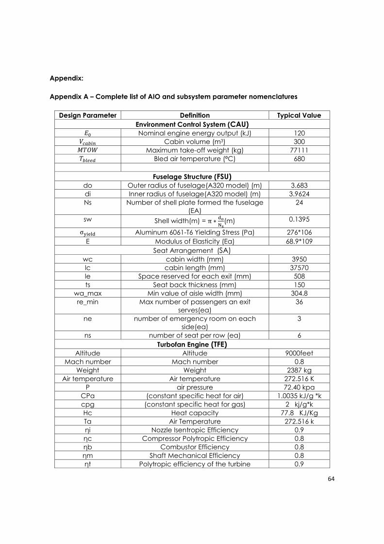
64

Appendix:

Appendix A – Complete list of AIO and subsystem parameter nomenclatures

Design Parameter Definition Typical Value Environment Control System (CAU)

Nominal engine energy output (kJ) 120 Cabin volume (m3) 300 Maximum take-off weight (kg) 77111

Bled air temperature ( C) 680

Fuselage Structure (FSU) do Outer radius of fuselage(A320 model) (m) 3.683 di Inner radius of fuselage(A320 model) (m) 3.9624 Ns Number of shell plate formed the fuselage

(EA) 24

sw Shell width(m) = (m) 0.1395

Aluminum 6061-T6 Yielding Stress (Pa) 276*106 E Modulus of Elasticity (Ea) 68.9*109

Seat Arrangement (SA) wc cabin width (mm) 3950 lc cabin length (mm) 37570 le Space reserved for each exit (mm) 508 ts Seat back thickness (mm) 150

wa_max Min value of aisle width (mm) 304.8 re_min Max number of passengers an exit

serves(ea) 36

ne number of emergency room on each side(ea)

3

ns number of seat per row (ea) 6 Turbofan Engine (TFE)

Altitude Altitude 9000feet Mach number Mach number 0.8

Weight Weight 2387 kg Air temperature Air temperature 272.516 K

P air pressure 72.40 kpa CPa (constant specific heat for air) 1.0035 kJ/g *k cpg (constant specific heat for gas) 2 kj/g*k Hc Heat capacity 77.8 KJ/Kg Ta Air Temperature 272.516 k

i Nozzle Isentropic Efficiency 0.9 c Compressor Polytropic Efficiency 0.8 b Combustor Efficiency 0.8 m Shaft Mechanical Efficiency 0.8 t Polytropic efficiency of the turbine 0.9

65

j Isentropic efficiency of the nozzle 0.9 t Turbine pressure ratio 0.8 in Intake air pressure ratio 1 t turbine temperature ratio 0.4579 in Intake temperature ratio 1

Ra Air Gas Constant 0.287 KJ/kg K Rg Fuel Gas Constant 0.189 KJ/kg K

A Air Density 1.2920 kg/m3 g Fuel Density 817.15 kg/m3

H Enthalpy of combustion of air 43.1 Mj/kg D Diameter of fan 1.587 m

AIO system parameters Wavg_p Average Passenger Weight 80 kg $ticket Ticket Price 200 USD $fuel Fuel Price 1 USD/kg tflight Flight Time 18000 s