Profiting from Mean-Reverting Yield Curve Trading Strategies

Choong Tze Chua Corresponding Author

Lee Kong Chian School of Business Singapore Management University

50 Stamford Road, Singapore 178899 Tel: +65.6828.0745

Email: ctchua@smu.edu.sg

Winston T.H. Koh School of Economics and Social Sciences

Singapore Management University 90 Stamford Road, Singapore 178903

Tel: +65.6828.0853 Email: winstonkoh@smu.edu.sg

Krishna Ramaswamy The Wharton School

University of Pennsylvania 3259 Steinberg-Dietrich Hall, Philadelphia, PA 19104

Tel: 215.898.6206 Email: krishna@wharton.upenn.edu

23 Jan 2006

JEL Classification number: C41, E43, G14

Keywords: yield curve, fixed income trading, market efficiency, Treasury bonds

Support from the Wharton-SMU Research Centre, Singapore Management University is

gratefully acknowledged. The authors would also like to thank Dean Foster, Mitchell Craig

Warachka, Jun Yu and seminar participants at Singapore Management University, the 2004

Econometric Society meeting in Melbourne and the 2005 Financial Management Association

meeting in Siena for their valuable comments.

Profiting from Mean-Reverting Yield Curve Trading

Strategies

ABSTRACT

This paper studies a set of yield curve trading strategies that are based on the view

that the yield curve mean-reverts to an unconditional curve. These mean-reverting

trading strategies exploit deviations in the level, slope and curvature of the yield

curve from historical norms. Some mean-reverting strategies were found to have

significant positive profits. Furthermore, the profitability of one of these strategies

significantly outperforms, on a risk-adjusted basis, alternative strategies of an

investment a bond or equity index.

1

Trading in fixed income assets is a profitable business in global investment

banks. Besides providing market liquidity through market-making activities, investment

banks also devote significant amounts of proprietary capital to trade a wide variety of

fixed income instruments, such as Treasury bills to 30-year government bonds,

corporate bonds and mortgage-backed securities, etc. Besides investment banks, hedge

funds and dedicated bond funds also actively pursue trading opportunities in fixed

income assets.

The strategies deployed range from simple arbitrage-trading, to complex trades

based on technical or market views on the term structures of interest rates and credit

risks. These yield curve trading strategies are essentially bets on changes in the term

structure. These trading strategies can be broadly classified as directional and relative-

value plays. Directional trading, as the name implies, are bets on changes in the interest

rates in specific directions. Relative-value trading, by contrast, focuses on the market

view that the unconditional yield curve is upward sloping, and that the current yield

curve would mean-revert to an unconditional yield curve. A wide variety of trading

techniques are used to construct relative-value trades based on this market view.

However, there have been few efforts to examine the performance of these trading

strategies or to compare them with equity investment strategies. Litterman and

Scheinkman [1991], Mann and Ramanlal [1997] and Drakos [2001] are recent studies

on the subject.

In this paper, we analyze the performance of a specific class of such relative-

value trading techniques that are directly implied by the notion that mean-reversion of

the yield curve occurs. We consciously avoid “data-snooping” by not searching through

a large number of possible strategies to find a few that are profitable. Instead, we start

2

from the market view that the yield curve mean-reverts and derive trading strategies

that follows most naturally from such a view—if the level, spread or curvature is higher

(lower) than the historical average, bet that the level, spread or curvature, respectively,

will decrease (increase) towards the historical average. We shall refer to this class of

technical trading strategies as “mean-reverting” trading strategies. Following Litterman

and Scheinkman [1991], we consider the three aspects of the yield curve – namely, the

interest rate level, the slope (i.e. yield spread) and the curvature – and construct a

portfolio of yield-curve trading strategies centering on each aspect. To facilitate a

consistent comparison of their performance, we impose cash neutrality and consider

one-month holding period for each category of strategies, and adjust the payoff for risk,

as measured by the standard deviation of the payoffs. Our study abstracts from credit

risk --in particular, default risk – and chooses as our dataset, the U.S. Treasury interest

rates, from the period 1964 to 2004 for our study. For each aspect of the yield curve, we

consider strategies that trade on the whole yield curve, as well as strategies that trade on

individual portions of the yield curve.

Our analysis shows that there exists a set of mean-reverting trades that appear to

offer, on average, superior payoffs, even after accounting for transaction costs, over the

period considered in our study. We compare these payoffs to two benchmarks. The first

benchmark is a cash-free investment in the Lehman Brothers Government Intermediate

Index. This involves essentially buying the index, which consists of a portfolio of

bonds with maturities ranging from 1 year to 10 years, and selling short 1-month U.S.

Treasury Bills, thereby earning the term premium (see Stigum and Fabozzi [1987], pp

271). The second benchmark involves a risk-adjusted strategy of investing in the S&P

index, and funding the trade also by shorting one-month U.S Treasury bills. In this

3

comparison, we found that some yield curve strategies outperform the S&P strategy by

up to 5.7 times, and the Lehman Brothers Bond index strategy by up to 4.8 times, based

on a comparison of the risk-adjusted average gross payoffs.

While factoring in trading costs may appear to diminish the profits from some

of the mean-reverting yield curve trades (one of the strategies still return profits that

were significantly higher than the benchmarks, even after accounting for transaction

costs), we must add that the implied transaction cost we calculated is based on the

assumption of actually trading the whole principal value of the Treasury securities. The

transaction costs can be significantly reduced by structuring derivative trades on a

notional basis, mirroring the economic cash flows of the underlying yield curve trades

but without actually funding and holding the bonds. These derivative trades are

commonly carried out in the fixed income market. Hence, the potential remains for

more mean-reverting yield curve strategies to yield significant positive returns.

MEAN-REVERTING YIELD CURVE STRATEGIES

There is a wide variety of yield curve trading strategies. The literature on yield

curve trading dates back to the late 1960s; a sample of the earlier literature includes De

Leonardis [1966], Freund [1970], Darst [1975], Weberman [1976], Dyl and Joehnk

[1981] and Stigum and Fabozzi [1987]. More recent analysis of the subject are found in

Jones [1991], Mann and Ramanlal [1997], Grieves and Marchus [1992], Willner [1996]

and Palaez [1997].

Our focus in this paper is on yield curve trading strategies that are based on the

conventional view that the yield curve mean-reverts to some historical norm. This

4

market view is consistent with historical experience. For instance, U.S. Treasury bill

rates, spreads and curvature all trade within tight, finite bounds. The interest rate term

structures in other countries also exhibit similar patterns. This suggests that some form

of mean-reversion mechanism is at work that prevents the yield curve from drifting to

extreme levels or shapes over time.

The market view of yield curve mean-reversion is also represented in theoretical

models of the interest rate term structure – as discussed in Vasicek [1977], Cox,

Ingersoll and Ross [1981, 1985], and Campbell and Shiller [1991], for example – which

incorporate some form of mean-reversion mechanisms and are based on some form of

the expectations hypothesis.1 In essence, the pure expectations hypothesis of the term

structure is the theory that the long-term interest rate is the average of the current and

expected short-term rates, so that the yield spread is mean-reverting.2 Interest rates

along the yield curve adjust to equalize the expected returns on short- and long-term

investment strategies.3 Furthermore, by incorporating rational expectations, the pure

expectations hypothesis implies that excess returns on long bonds over short bonds are

un-forecastable, with a zero mean in the case of the pure expectations hypothesis. Any

arbitrage opportunity should be captured and realized by investors immediately.

Therefore, by the pure expectations hypothesis, yield curve trading strategies

1 Shiller [1990], Campbell [1995] and Fisher [2001] provide surveys of the literature on interest rate term

structure.

2 This was first propounded by Fisher [1986] and refined by Lutz [1940] and Meiselman [1962].

3 A weaker version, referred to as the expectations hypothesis, states that the difference between the

expected returns on short- and long-term fixed income investment strategies is constant, although it need

not be zero as required under the pure expectations hypothesis.

5

attempting to exploit anomalies or mis-pricings in the term structure would not yield

consistently positive payoffs.

The expectations hypothesis of the term structure, therefore, stands in contrast

to the practitioner’s view that it is possible to construct mean-reverting yield curve

trading strategies to generate consistent positive payoffs. Broadly speaking, mean-

reverting yield curve strategies attempt to take advantage of deviations in the current

yield curve relative to an unconditional yield curve. Three commonly-used trades are:

(a) bullet strategy, which is constructed so that maturities of bonds are concentrated at a

particular part of the yield; (b) ladder strategy, which involve investments across a

range of maturities; and (c) barbell strategy, which are constructed, for example, by

investing in two ends of the yield curve, and shorting the middle portion, or vice versa

(see Fabozzi [1996]). It is easy to see that bullet strategies are essentially bets on the

level of the interest rates, while ladder strategies and barbell strategies are bets on the

yield spreads and curvatures, respectively.

There have not been systematic efforts to examine the performance of these

trading strategies, and relate them to the predictions of the expectations hypothesis. An

exception is Culbertson [1957] who computed and graphed holding period returns,

between one week and three weeks, for short and various long term Treasury securities.

He found that the holding period returns were very different from observed spot interest

rates, and concluded that the pure expectations hypothesis, as propounded by Lutz

[1940] did not hold.

The predictability of the spot yield curve and the forward interest rates, as

implied by the expectations hypothesis, has also not found unambiguous empirical

support (see Hamburger and Platt [1975]). Shiller, Campbell and Schoenholtz [1983]

6

showed that the term structure does not provide information on the future change in the

short-term rates. Moreover, as Cox, Ingersoll and Ross [1985] first showed, the

different versions of the expectations hypothesis are not theoretically consistent.

Mankiw and Miron [1986] also found that the predictability of the term structure

disappears after the founding of the Federal Reserve. Subsequent work by Rudebusch

[1995] and Balduzzi, Bertola and Foresi [1997] also found that changes in the interest

rate were due to unexpected changes in the Fed targeting.

Data

The dataset we use for our study is the Fama-Bliss dataset obtained from CRSP

(Centre for Research in Securities Prices, 2004). The data set contains monthly data on

zero coupon yields derived from a yield curve of U.S. government Treasury bills and

bonds from 30 June 1964 to 31 December 2004. We acknowledge that zero coupon

yield data derived from the US Treasury markets prior to the mid 1980’s might contain

some systematic biases.

We first note that many of the bonds in that period are callable bonds; thus, the

price of the bond includes the value of the call option. These bonds are also likely to

possess tax effects that are different from pure zero-coupon bonds (since STRIPS only

start to trade actively from the mid-1980’s onwards). The liquidity of these bonds was

also relatively low and could result in a liquidity premium being priced in. However, all

these factors contributed to systematic bias in the price and yields; therefore, they

should have only a tangential effect on our results. This is the case since the strategies

we considered are always long-short strategies: for every bond that we go long in, we

short another bond with the same value to maintain zero initial cash-flow. Moreover,

7

the decisions to long or short bonds at specific tenors are based on comparisons with

historical averages. If the historical averages are similarly biased, then the results

should be unaffected by the bias. Also, any bond of any tenor is, unconditionally,

equally likely to be shorted as it is to be longed at any point of time. Therefore,

systematic biases in the relative valuation between 2 bonds (for instance, if short

maturity bonds were to be consistently undervalued relative to longer maturity bonds)

should not bias the overall direction of the result when summed over the time series. In

aggregate, due to the large number of both long and short trades made across different

bonds and time, we have good reasons to believe that the data quality issue before the

mid 1980s would not present a bias in our results in any particular direction. In fact, the

noise created by this data quality issue may have caused the true level of significance to

be understated.

For the purpose of this study, we express all zero coupon yields in the form of

continuously compounded yields. These zero-coupon yields are of maturities that are

approximately 1-month, 2-month, … , 12-month, 24-month, 36-month, 48-month and

60-month. The observed maturities are approximate in the sense that some bonds may

be of 0.9 month, 3.3 month or 11.8 month in maturities. Moreover, the observation

interval for each yield curve is only approximately one-month apart (e.g. 28 days or 33

days). The total number of time-series yield curve observations in our dataset is 487.

For the purpose of our study, we regularize the dataset. This is carried out in

two steps. First, we perform a cross-sectional linear interpolation to each zero yield

curve in order to obtain the yields at exact monthly tenors from 1-month to 60-month.

For instance, if the observed yields are 9.8 months, 11.3 months and 12.3 months, we

interpolate linearly to obtain the yields for the 10-month, 11 month and 12-month

8

tenors. Also, we linearly interpolate to obtain yields for maturities of 13-months, ... ,

23-month, 25-month, ... , 35-months, 37-months, ... , 47-months and 49-months, ... , 59-

months based on observed yields for months 12, 24, 36, 48 and 60. For our analysis, we

shall refer to bonds with yields that are observed in the market as ‘primary’ bonds, and

bonds with maturities that are not observed in the market as ‘hypothetical’ bonds.

Hypothetical bonds therefore have maturities greater than 12 months, but are not

divisible by 12. The distinction is made to facilitate a comparison of alternative yield

curve strategies in our analysis.

The second step that we took to regularize the dataset is a temporal linear

interpolation procedure. The following example explains the procedure. Suppose the

interpolated 13-month yield are observed at three dates, 7% (date 0), 7.5% (28 days

later) and 6% (another 33 days later). Since we focus on a holding period of one month,

we require the yield curves to be at exactly one-month intervals, in order to calculate

the payoff at the end of each holding period. For our purpose, we define this to be

365.25 days divided by 12, i.e. 30.4375 days. Hence, the temporally interpolated 13-

month yield in this example are 7% (date 0), 7.3892% (30.4375 days) and 6.0057%

(another 30.4375 days later).

Since the holding period of each trade is one-month, the relevant forward yield

curve with which to compare against the unconditional yield curve is the one-month

forward yield curve. The one-month forward interest rate at a maturity of X months is

calculated as follows. Let denote the current interest rate while denote the one-

month forward interest rate. We have

,0Xr ,1Xr

,1 1,0 1,0

1 112 12 12x xx xr r r

e e e ++

⋅ = (1)

9

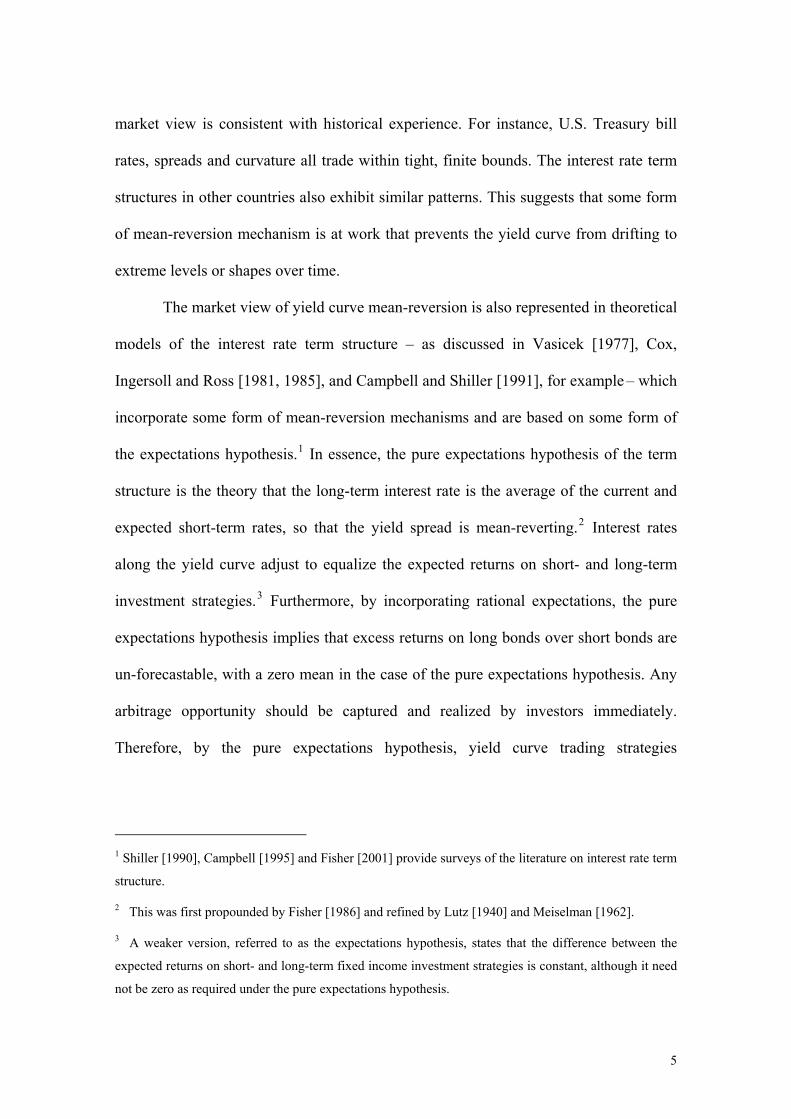
Finally, the unconditional yield at each maturity (for primary and hypothetical

bonds) at any date is calculated as the simple average of all the yields observed for that

maturity since June 1964 till the preceding month. We define the unconditional yield

curve at any date as the set of unconditional yields over all the maturities. Exhibit 1

below illustrates the unconditional yield curve for various dates.

---------------------------------------------------

INSERT EXHIBIT 1 HERE

--------------------------------------------------

Strategies

We consider three classes of mean-reverting yield curve strategies, focusing on

the three aspect of the yield curve: level, slope (i.e. yield spread) and curvature. For

each strategy, the holding period of a trade is fixed at one month, after which a new

trade is initiated. We impose cash neutrality, so that any excess cash is deposited at the

1-month tenor. Similarly, if additional funding is required, this is carried out at the 1-

month tenor. Since the holding period is 1 month, a bond of maturity X months has

duration (X− 1) months. Consequently, the deposits and borrowings at the one-month

tenor have no impact on the duration of each trade—interest rate movements have no

effect on deposits and borrowings at the one-month tenor. We recognize that borrowing

at Treasury bill rates is usually impossible; however the cash-neutrality design of our

study makes actual shorting of Treasury bills unnecessary. Whenever a Treasury bill

needs to be shorted, we will correspondingly need to go long on some other Treasury

security. The combined effect of these two transactions can be achieved via a derivative

10

such as Treasury forwards and futures. Stringing together a series of Eurodollar futures

can also produce a good approximation to the required cash-flows. For the S&P Index

strategy, a position in the S&P futures will generate the required cash-neutral

investment without actually shorting any Treasury Bills.

We allow for a 102-month training period in the construction of the

unconditional yield curve, so that our calculation of the average payoff of each yield-

curve strategy starts from January 1973 to December 2004. The reason for the selection

of this particular training period is the fact that the Lehman Brothers U.S. Government

Intermediate Bond Index, which is one of our benchmarks, starts in January 1973.

Class 1: Mean-reversion of yield levels

This class of yield-curve trading strategies is based on the view that the level of

the yield curve mean-reverts to the unconditional level. We consider two strategies.

Strategy 1-A: Mean-reversion of average yield to the unconditional average

This strategy takes the view that the average level of the yield curve mean-

reverts to that of the unconditional yield curve. In this trade, we compare the average of

all the one-month forward yields at a particular date against the corresponding average

for the unconditional yield curve. If the average interest rate level for the one-month

forward yield curve is higher (lower) than the average for the unconditional yield curve,

the expectation is that one-month forward yield curve would shift down (up). The

implied strategy is to go long (short) all the bonds with maturities longer than one

month. We consider two versions of the trade, one for maturities of only primary bonds,

and another for all maturities, including all the interpolated maturities of the

hypothetical bonds.

11

The trade is constructed as follows. If k/59 dollars are invested in the 60-month

bond, with a duration of 59 months over the one-month holding period, the amount of

cash invested in a bond of maturity of X months, with duration of (X− 1) months, will

be k/(X− 1) dollar. The funds required to invest in all the bonds are borrowed at the

month tenor. Similarly, if the trade is to go short all the bonds, then the cash is

deposited in the one-month tenor. Therefore, the strategy is a duration-weighted, cash

neutral trade. In this strategy, a parallel shift in the yield curve generates approximately

equal contribution to the payoff at each maturity.

Strategy 1-B: Mean-reversion of yield at each maturity to its unconditional level

This strategy is based on the view that the yield at each maturity mean-reverts to

its unconditional level. In this trade, if the one-month forward yield is higher (lower)

than the corresponding level on the unconditional yield curve, the expectation is that

one-month forward yield curve would fall (rise). Except for the one-month maturity,

the implied strategy is to go long (short) the bond. The trade is constructed so that a

parallel shift in the yield curve generates approximately equal contribution to the payoff

at each maturity. If we go long or short k/59 dollars in the 60-month bond, the amount

to long or short a bond of maturity of X months, with duration of (X− 1) months will be

k/(X− 1) dollar. Again, the one-month sector is where deposits and borrowings are

made to achieve cash neutrality. We consider two versions of the trade, one for

maturities of only primary bonds, and another for maturities, including all the

interpolated maturities of the hypothetical bonds.

Class 2: Mean-reversion of yield spreads

12

In this strategy, the focus is on the mean reversion of the slope of the yield

curve. Two versions of the trade are carried out.

Strategy 2-A: Mean-reversion of yield spread for the whole yield curve

The trade is constructed as follows. Consider the spread between the 59-month

and 1-month maturities on the one-month forward yield curve, and compare it with that

of the unconditional yield curve. If the one-month forward yield spread is larger

(smaller) than the historical average, the expectation is that the slope of the yield curve

would fall (rise). The implied strategy is to go long (short) the 60-month bond and go

short (long) the 2-month bond.

The trade is constructed as follows. Suppose k/59 dollars are invested in the 60-

month bond, we need to short the 2-month bond by k dollars, to achieve duration-

matching. The excess cash of 58k/59 dollars is deposited in the one-month tenor. This

strategy is a cash neutral trade and has a zero net duration. A parallel shift in the yield

curve has negligible impact on the payoff.

Strategy 2-B: Mean reversion of the yield spreads between 2 adjacent bonds.

This trade is based on the view that the yield spread between two adjacent bonds of

maturities (X−1) months and (Y−1) months, with Y > X, on the one-month forward

yield curve would mean-revert to the corresponding spread on the unconditional yield

curve. We compare the yield spread of adjacent pairs of bonds on the one-month

forward yield curve against the historical average on the unconditional yield curve. If

the one-month forward spread is larger (smaller) than that for the unconditional curve,

go long the bond, with maturity of Y months, and short the bond with maturity of X

months. We duration-weight each leg of the trade so that changes in the yield spread

13

with equal magnitude across different trades would generate approximately equal

payoff contribution to the portfolio. For any bond with maturity of Z months, the cash

to go long or short the bond is k/(Z−1) dollars. We again impose cash neutrality.

This trade essentially focuses on the slope of the yield curve for adjacent bonds

on the one-month forward yield curve. We consider two versions of the trade, for both

yield curves with only primary bonds and another set with maturities one month apart

from one month to 60 months.

Class 3: Mean reversion of curvature

We define curvature as follows. Take three zero coupon bonds, with maturities

of X, Y and Z months and corresponding one-month forward yields of , and Xr Yr Zr .

The curvature of the curve yield curve, as defined by the three bonds, is the measure:

( , , )c X Y Z ≡ Y X Z Yr r r rY X Z Y

− −−

− − (2)

If the curvature is smaller (larger) relative to the corresponding measure for the

unconditional yield curve over the same set of maturities, the expectation is that the

curvature of the one-month forward yield curve would increase (decrease). We consider

two strategies.

Strategy 3-A: Mean reversion of the curvature of the yield curve

This strategy focuses on the entire yield curve. Specifically, we consider the

maturities of 1-month, 29-month (a hypothetical bond, and the mid-point) and the 59-

month bond, on the one-month forward yield curve. If the curvature is expected to

increase (decrease), the implied trade is to go long (short) the 2-month and 60-month

bond and short (long) the 30-month bond, on the current yield curve. We match the

14

durations of the various portions of the trade as follows. For every k/59 dollars invested

in the 60-month bond (with a duration of 59 months), the amount invested in the 2-

month bond is k dollars. Next, for the 30-month bond (with a duration of 29 months),

the amount to short is 2k/29 dollars. The excess funding needs is met by borrowing k

(1/59 + 1 − 2/29) dollars at the one-month tenor. The trade is cash-neutral and has zero

duration, so that a parallel shift in the yield curve or a change in the slope of the yield

curve without a change in curvature has negligible impacts on the payoff. The curvature

trading strategy we just described is often referred to as a barbell strategy.

Strategy 3-B: Mean reversion of the curvature of 3 adjacent bonds to the unconditional

curvature

In this trade, we compare the curvature of any three adjacent bonds, say with

maturities of (X−1), (Y−1) and (Z−1) months on the 1-month forward yield curve, as

measured by described in (2), with the corresponding curvature by

the unconditional yield curve. If the curvature is smaller (larger) relative to that for the

unconditional yield curve, the expectation is that the curvature of the current yield

curve over the three maturities would increase (decrease). The implied trade is go long

(short) the X-month and Z-month bond and short (long) the Y-month bond.

( 1, 1, 1c X Y Z− − − )

Again, we match the durations of the various portions of the trade so that the

trade is immune to shifts in the yield curve. The amount of cash to be invested in the X-

month and Z-month bonds are, respectively, k/(X−1) dollars and k/(Z−1) dollars. As for

the bond with Y-month maturity, the cash amount is given by 2k/(Y−1) dollars. The

funding need or excess cash for this trade is k/(X−1) + k/(Z−1) – 2k/(Y−1) dollars. The

strategy is essentially a portfolio of curvature trades, using all the primary bonds.

15

Since the hypothetical bonds are linearly interpolated from the primary bonds,

the curvatures of the hypothetical bonds are zero. Hence, the trade does not work with

hypothetical bonds.

Benchmarks

In order to be able to compare the performance of the mean-reverting trades

described in the preceding subsection, we construct two benchmarks. The first is a

fixed income strategy benchmark while the second is an equity investment benchmark.

Benchmark 1 – Investment in the Lehman Brothers U.S. Government Intermediate

Bond Index 4

This benchmark is constructed by assuming that we go long on the Lehman

Brothers U.S. Government Intermediate Bond Index. The trade is funded by shorting 1-

month Treasury bills. This is a standard benchmark in the fixed income market,

essentially deriving its returns from the term premium of interest rates (see Stigum and

Fabozzi [1987]). This trade, like all the other strategies that we are testing, is cash

neutral. When used as a benchmark, we will match the volatility of this strategy to the

other strategies, and then compare the means.

4 There is a similar, though less common, benchmark that we can use. Profiting from the term premium

involves buying a long-dated bond, and holding it for a period of time. Therefore, a logical benchmark is

to simply buy a 60-month bond every month and holding it to maturity, all the while repeatedly funding

the long positions with corresponding short positions in the 1-month Treasury Bills. A new 60-month

bond is bought each month. Hence, at any one time, there is portfolio of bonds of maturities ranging

from one month to 60 months. The payoff of the portfolio is calculated as the marked-to-market profits

each month. As expected, this benchmark is almost identical to an investment in the Lehman Brothers

U.S. Government Intermediate Bond Index.

16

Benchmark 2 – Cash-neutral Investment in S&P Index

Finally, we construct an equity benchmark to compare the performance of

mean-reverting trades against an alternative investment strategy in equity assets. Most

studies on fixed income investment strategies do not compare the performance against

the alternative strategy of investing in equity instruments. Any attempt at doing so often

runs into problems of comparability, in terms of risk adjustments, holding period and

credit risks etc. The equity benchmark we construct addresses these issues.

We use the S&P index, starting from January 1973. Invest a dollar in the S&P

index, and borrow a dollar for one-month by shorting 1-month Treasury bills. The trade

is cash-neutral, with a one-month holding period. We found that the average profit is

$4.91 for every $1000 invested in the S&P, funded by 1-month borrowings – the

average monthly excess returns of the S&P index over our sample period is 0.491% per

month.

RESULTS AND ANALYSIS

By adjusting the cash amounts, we can derive comparable volatilities (standard

deviation) in payoffs for the S&P investment against a particular mean-reverting yield

curve strategy. Let the standard deviation of payoffs for the cash-neutral investment in

the S&P index from January 1973 to December 2004 be denoted by Eσ (the standard

deviation of the monthly excess returns of the S&P index). Similarly, let #σ denote the

standard deviation of payoffs from a $1 nominal position for a yield curve strategy

numbered #, from January 1973 to December 2004. Hence, to yield identical volatility

in payoffs, the cash amount of k dollars for a particular yield curve strategy is given by

17

#

Ek σ

σ= (3)

for each dollar invested in the S&P trade. Note that the matching of volatilities across

different strategies is done after all the payoffs are realized. This is to ensure that the

volatilities of the 2 competing strategies will be matched exactly. This procedure does

not, in any way, compromise the fact that all investment decisions are made “out-of-

sample”. It merely seeks to evaluate any two competing strategies on a fair and

comparable basis by scaling the size of the monthly payoffs to match the standard

deviations of the 2 strategies.

Exhibit 2 below presents performance of the various strategies and benchmarks

before accounting for trading costs (We defer the discussion of transaction costs to a

later section). From Exhibit 2, we note that, on a comparable risk-adjusted basis, only

strategies 2-B, 3-A and 3-B yield higher payoffs compared with the two benchmarks. In

particular, not all mean-reverting yield curve strategies beat the simple buy-and-hold

bonds strategy (Benchmark 1). In the following subsections, we analyze in detail the set

of profitable mean-reverting yield-curve strategies.

---------------------------------------------------

INSERT EXHIBIT 2 HERE

--------------------------------------------------

Performance against the Benchmarks

Against the two benchmarks, strategies 2-B and 3-B have performed

remarkably well. On a comparable basis, Exhibit 2 shows that the monthly payoff of

18

strategy 2-B is about 5.7 times that of the monthly payoff of the equity benchmark

(benchmark 2). This means that while investing $1000 in S&P (and funding the

investment by shorting 1-month Treasury Bills) generates an average profit of $4.91

per month, strategy 2-B generates $27.78 per month, after adjusting the volatility of

payoffs for strategy 2-B to exactly match the volatility of payoffs from the S&P

strategy. For strategy 3-B, the corresponding ratio is about 3.9 times against the equity

benchmark. Hence, yield-spread mean-reverting and curvature mean-reverting

strategies can outperform an equity investment strategy, on a risk-adjusted basis.

Moreover, Strategies 2-B and 3-B also outperformed the bond benchmark. In

the case of strategy 2-B, the average monthly payoff is about 4.8 times that of

Benchmark 1, while for strategy 3-B, the average monthly payoff is about 3.3 times

that of Benchmark 1.

The next subsection will test whether these superior performance of (gross)

payoffs relative to the benchmarks are statistically significant.

Test of Significance of Excess Payoffs against Benchmarks

To test whether strategies 2-B, 3-A and 3-B significantly outperform the

benchmarks, we conduct two statistical tests of significance; these are: the paired t-test

and the z-test using the Newey-West estimator (Hereafter, N-W test, Newey and West

[1987]. Also see Diebold and Mariano [1995] for another possible test of significance

for auto-correlated series).

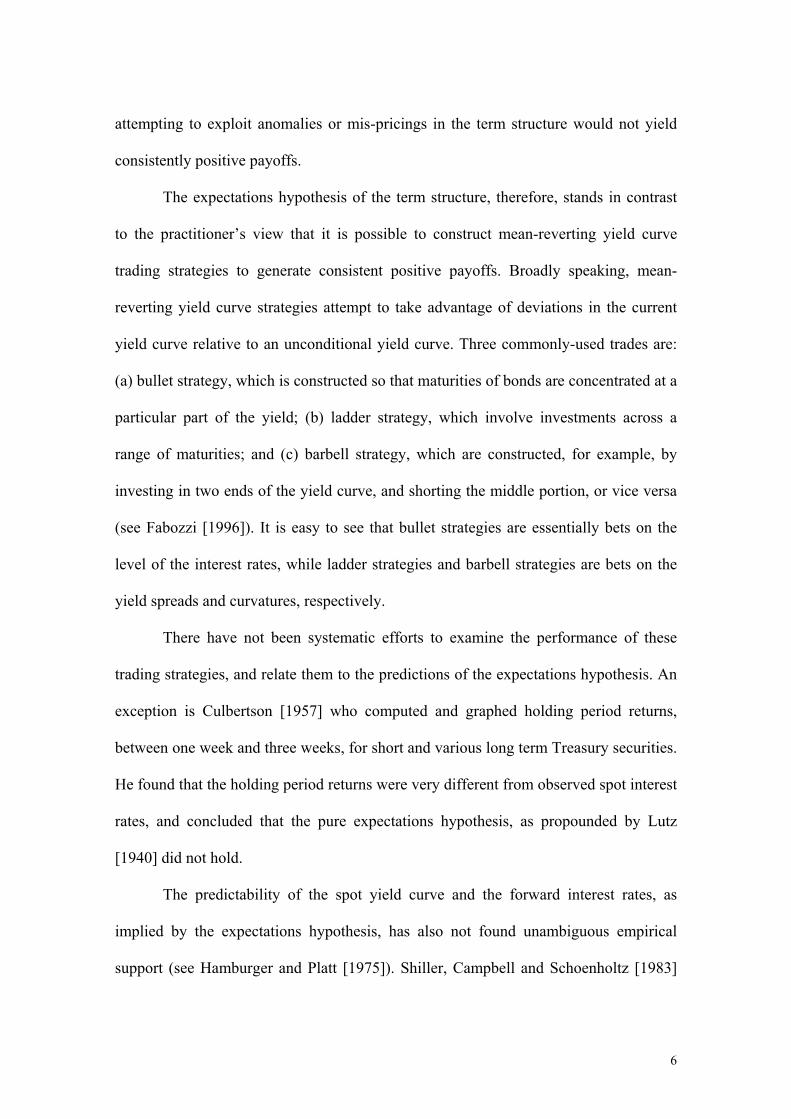
The paired t-test requires that the time-series of payoff differences be

uncorrelated. Positive auto-correlations will incorrectly overstate the power of the test.

Exhibits 3, 4 and 5 respectively plot the first 60 auto-correlation of the payoff

19

differences between the strategies and the benchmarks. The autocorrelations are small

in absolute values and are also distributed across positive and negative values. This

means that the paired t-test, while not perfect, is still reasonable for our purpose.

----------------------------------------------------

INSERT EXHIBITS 3, 4 AND 5 HERE

---------------------------------------------------

The Newey-West estimator can be used to ascertain whether the mean of an

autocorrelated and heteroskedastic series is significantly different from zero. It is less

powerful that the t-test, but it requires weaker assumptions by accounting for auto-

correlation. We also allow autocorrelations of up to 60 lags. The Newey-West

generates a variance estimate that can then be used to compute the z-score for a

particular series. Therefore, a statistic higher than 1.96 will imply that the difference

between the two means being tested is statistically significant.

---------------------------------------------------

INSERT EXHIBIT 6 HERE

--------------------------------------------------

Exhibit 6 shows that while strategy 3-A does not significantly outperform the

benchmarks, strategies 2-B and 3-B do. In particular, the p-value of the t-tests for

strategies 2-B and 3-B are negligible. For the Newey-West test, strategy 2-B managed a

p-value of 0.002 and 0.001 against benchmarks 1 and 2 respectively; while strategy 3-B

20

obtained a p-value of 0.013 and 0.008 against benchmarks 1 and 2 respectively. These

p-values of these tests for strategy 2B are so low that our results are still highly

significant even after making simple bonferroni adjustments to account for the fact that

we tested 6 strategies in this study.5

Having a profitability that is not significantly more than the benchmarks, but

that is significantly more than zero could still mean that the strategy is useful as a

positive-mean diversification tool if the correlations with the benchmarks are low. This

is indeed the case for the strategies in this study. For all 3 strategies, the profitability is

significantly more than zero for both the t-test as well as the N-W test. The correlations

between the profits of the strategies and both the benchmarks are also extremely low.

For strategy 2-B, the correlations of profits with benchmarks 1 and 2 are 0.0258 and

0.0567 respectively. For strategy 3-A, the correlations of profits with benchmarks 1 and

2 are -0.2188 and 0.0453 respectively. For strategy 3-B, the correlations of profits with

benchmarks 1 and 2 are 0.0670 and -0.0028 respectively.

Transaction Costs

Thus far, all our analyses are done in terms of the gross payoffs of the different

mean-reverting yield curve strategies. An obvious question to ask is whether the set of

profitable trades, specifically strategies 2-B and 3-B, would continue to outperform the

indices (or even yield positive returns) when the appropriate transaction costs are taken

into account. Transaction costs in bond trading are embedded in the form of the spread

5 The simple bonferroni correction adjusts the required p-value for rejection to account for multiple tests

by dividing the alpha-level by the number of tests conducted. Therefore, in the case of our study where 6

tests are conducted, the p-value required for a rejection at the 5% level is 0.008333. The p-value from

Strategy 2-B is still smaller than 0.00833.

21

between the ‘bid’ and ‘ask’ yields. The 5-year average spreads are approximately 1

basis point for Treasury bills that mature in 1 year or less, 0.8 basis points for 2-year

bonds and 0.35 basis points for 5-year bonds6. A reasonable assumption would be that

the effective transaction cost for each trade is half the quoted spread. For the purpose of

this paper, we assume a spread of 3 basis points for all the bonds traded from Jan 1973

to Dec 1980, 2 basis points for all bonds traded from Jan 1981 to Dec 1990 and 1 basis

point for all bonds traded from Jan 1991 to Dec 2004 (and therefore pay a transaction

cost of 1.5, 1 and 0.5 basis points respectively). Assuming a cost of 1 basis point, the

cost expressed in dollars is a function of the maturity of the bond and the value of the

bond, and can be approximated as follows7:

(Transaction Cost) ≈ 0.0001 * (Maturity in Years) * (Value of Bond) (4)

As an illustration, buying or selling $100,000,000 worth of 6-month Treasury

Bills will attract a transaction cost of 0.0001*0.5*$100,000,000 = $5,000.

---------------------------------------------------

INSERT EXHIBIT 7 HERE

----------------------------------------------------

The profitability of strategies 2-B, 3-A and 3-B after accounting for transaction

costs are reported in Exhibit 7. We assume that the benchmarks are traded without any

6 Source: Bloomberg, accessed on 5 November 2003. 7 Assume a yield of r for the bond with T years to maturity. If we were to buy the bond, based on a 1 basis point transaction cost, we obtain a yield of (r-0.0001). Thus, the transaction cost, in dollar terms would be: e-(r-0.0001)T – e-rT = e-rT (e0.0001T-1) ≈ e-rT (1 + 0.0001T-1) = 0.0001 * T * e-rT

22

transaction costs. Strategy 2-B is still significantly more profitable than both the

benchmarks under all measures (both the t-tests and the N-W tests). Both strategies 3-A

and 3-B no longer perform better than the benchmarks. However, the average profits

are still positive; and in the case of strategy 3-B, significantly so.

It is important to note that the transaction costs we calculated are based on the

assumption that the mean-reverting yield curve strategies are executed on a physical

basis, i.e. the actual bonds are bought and sold and funds are borrowed (if required) to

construct the trades on a monthly basis. The transaction costs can be diminished by

reducing the frequency of the entering and exiting trades. For instance, instead of

executing the trades on a monthly basis, the trades could be executed on a quarterly

basis, or when the relevant deviations on forward yield curves for spreads and

curvatures exceed certain thresholds.

More importantly, the transaction costs can be reduced substantially if the yield

curve strategies are structured as derivative trades (on a notional basis) to mirror the

economic cash flows of the underlying strategies, without actually funding and holding

the bonds. These derivative trades are commonly carried out in the fixed income

market.8 Therefore, while factoring in transaction costs may appear to diminish the

profits from some the mean-reverting yield curve trades, there are different ways to

lower the transaction costs. Nevertheless, Strategy 2-B still returns a significantly better

profit than all the benchmarks even after accounting for these costs.

8 Of course, the pricing of the derivative trades may involve other costs as well, as investment banks

take a cut from the potential profits. Fortunately, there are some standard derivatives that can be traded at

extremely low cost and can substitute for a pair of long-short trade in bonds. For instance, the highly

liquid Eurodollar futures gives identical payoff as shorting a bond of a certain maturity, and at the same

time going long a another bond of maturity 90 days longer than the shorted bond.

23

Value-Add of Mean-Reverting Strategy to Investment in the S&P Index

In the preceding sections, we have shown that a number of mean-reverting

yield-curve strategies can be highly profitable. Another way to demonstrate the

attractiveness of mean-reverting yield curve strategies is to consider the incremental

value-add of including such strategies to an existing investment strategy. In this regard,

Foster and Stine [2003] introduce a convenient test to ascertain whether a particular

strategy can add value to a buy-and-hold investment in the S&P index. The Foster-Stine

test is essentially a test on Jensen’s alpha (see Jensen [1968]), where the benchmark is

the S&P index-- it involves regressing the excess returns of the selected strategy against

the excess returns from the buy-and-hold investment in the S&P index. Based on this

regression, we can obtain the t-statistic as well as the p-value of the intercept that

allows us to test if adding a new strategy leads to a significant improvement in the

performance of the portfolio. Again, the critical p-value needs to be adjusted using the

bonferonni correction when multiple strategies are tested. If the regression intercept is

statistically significant, then we can infer that the particular strategy does in fact add

value to the original strategy of buy-and-hold the S&P index.

The basic premise behind this test is that a strategy that gives a positive mean

return and is not too highly correlated to the S&P index can be linearly combined with

the S&P index to obtain a better mean-variance return profile. In other words, a strategy

that serves as a good addition to diversify holdings in the S&P index can therefore add

value.

In the case of the mean-reverting yield-curve strategies we examined in this

paper, Strategies 2-B and 3-B are found to have significant value-add even after

accounting for transaction costs and the bonferonni correction. In particular, Strategies

24

2-B and 3-B have t-statistics of 6.816 and 2.685 respectively, with significant

corresponding p-values. The results of the Foster-Stine test are reported in Exhibit 8

below.

---------------------------------------------------

INSERT EXHIBIT 8 HERE

----------------------------------------------------

Breakdown of the Payoffs

Since strategy 2-B seems to be highly profitable, we find it necessary to

investigate the robustness of its profitability. As an initial check, we further analyzed

the breakdown of payoffs. Exhibit 9 shows the contribution of the payoffs from each

trade-segment in the portfolio for Strategies 2-B.

---------------------------------------------------

INSERT EXHIBIT 9 HERE

--------------------------------------------------

The results show that no single trade dominates the entire portfolio, and almost

all the trade segments generate positive payoffs. Interestingly, trading the yield spread

between 10-month and 11-month maturities on the one-month forward yield curve,

generate substantial positive profits while trading the yield spreads between 11- and 23-

months, as well as 23- and 35-months generate mild negative profits.

25

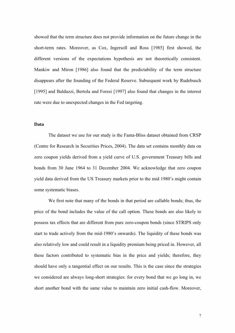
We also show the scatter-plot of the monthly payoffs against the absolute

deviations of the relevant parameter from the unconditional yield curve for trade-

segment 10—trading the 10-11 month spread. The scatter-plot is shown in Exhibit 10

below.

---------------------------------------------------

INSERT EXHIBIT 10 HERE

---------------------------------------------------

Exhibit 10 shows that, for this trade segment, the monthly payoffs have a high

positive correlation with the absolute deviations from the unconditional yield curve

(correlation = 0.819). In other words, the positive payoffs from this particular trade are

not random payoffs: the larger the deviation from the unconditional yield curve, the

larger the resulting profit from that particular trade. This result strongly supports the

view that the spread of these portions of the yield-curve do in fact mean-revert and the

reversion can be profitably exploited.

The presence of a very profitable trade segments in the 10-11 month portion of

the one-month forward yield curve followed by unprofitable trade segments from 11- to

35-months provides some support for the “market-segmentation” view of the interest

rate term structure in the fixed income market. This is the market view that many

participants in the fixed income market have preferred habitats that are dictated by the

nature of liabilities and investments, so that a major factor influencing the shape of the

yield curve is the asset-liability management constraints that are either regulatory or

self-imposed. Specifically, the yield curve is viewed as comprising a “short-end” – up

26

to the 12-month maturity – and a “long-end” – from 12-month onwards. Asset-liability

management constraints, when they exist, restrict lenders and borrowers to the short-

end or the long-end of the yield curve, or even certain specific maturity sectors, and, as

a result, investors and borrowers do not shift from one maturity sector to another to take

advantage of opportunities arising from differences between market expectations and

the forward interest rates. Arbitrage trades in the fixed income market are frequently

constructed in the transition between the short-end and the long-end of the yield curves.

Time Series Analysis

To investigate the profitability of strategy 2-B over time, we plot the 10-year

moving average of the payoffs of strategy 2-B as well as the two benchmarks. These

are shown in Exhibit 11 below.

---------------------------------------------------

INSERT EXHIBIT 11 HERE

---------------------------------------------------

From Exhibit 11, it can be seen that while the average monthly payoffs for

strategy 2-B stays significantly positive throughout the sample, the increasing

profitability of the benchmarks towards the end of the sample gradually eroded the out-

performance of the strategy over time. Nevertheless, the results remain significant, and

the absolute profitability (relative to zero) of the strategy does not seem to be sensitive

to the time period.

27

CONCLUSION

The objective of this paper is to examine the profitability of a range of yield-

curve trading strategies that are based on the view that the yield curve mean-reverts to

an unconditional yield curve. Our study has shown that a small number of these yield-

curve trading strategies can be highly profitable. In particular, trading strategies

focusing on the mean-reversion of the yield spreads significantly outperformed two

commonly-used benchmarks of investing in the Lehman Brothers U.S. Government

Intermediate Bond Index and investing in the S&P, on a risk-adjusted basis. Although

factoring in transaction costs lower the profitability of these trades against the

benchmarks, the significant result still remains for this strategy. Furthermore,

transaction costs can be reduced substantially, for instance, through structured

derivative trades that mirror the underlying cash flows or by reducing the frequency of

the trades.

We also investigate the profitability of these mean-reverting yield curve trades

over time. A time series analysis of the performance of the various yield-curve trading

strategies show that while the scope for excess returns over the benchmarks has

diminished over time, the absolute level of profitability has not suffered. Therefore,

profitable trading opportunities still exist (up to December 2004) in yield-spread mean-

reversion strategies. Moreover, these strategies as well as strategies that exploit the

mean-reversion of the curvature of the yield curve are found to have significant value-

add to a strategy of buy-and-hold the S&P index.

28

REFERENCES

Balduzzi, P., Bertola, G., and Foresi, S. “A model of target changes and the term

structure of interest rates.” Journal of Monetary Economics, 24 (1997), pp.371-399.

Campbell, J. “Some lessons from the yield curve.” Journal of Economic Perspectives,

9 (1995), pp.129-152.

Campbell, J., Shiller, R.J. “Yield spreads and interest rate movements: A bird’s eye

view.” Review of Economic Studies, 58 (1991), pp.495-514.

Culbertson, J.M. “The term structure of interest rates.” Quarterly Journal of Economics,

71 (1957), pp.485-517.

Cox, J.C., Ingersoll, J.E., Ross, S.A. “A reexamination of traditional hypotheses about

the term structure of interest rates.” Journal of Finance, 36 (1981), pp.769-799.

Cox, J.C., Ingersoll, J.E., Ross, S.A. “A theory of the term structure of interest rates.”

Econometrica, 53 (1985), pp.385-407.

Darst, D.M. The Complete Bond Book, (1975), McGraw Hill, New York.

De Leonardis, N.J. “Opportunities for increasing earnings on short-term investments,”

Financial Executive, 10 (1966), pp.48-53.

Diebold, F., Mariano, R.S. “Comparing predictive accuracy.” Journal of Business and

Economic Statistics, 13 (1995), pp.253-263,

Drakos, K. “Fixed income excess returns and time to maturity.” International Review of

Financial Analysis, 10 (2001), pp.431-442.

Dyl, E.A., Joehnk, M.D. “Riding the yield curve: does it work?” Journal of Portfolio

Management, 7 (1981), pp.13-17.

29

Fabozzi, F. J. Bond Markets, Analysis and Strategies, (1986), Upper Saddle River,

Prentice Hall, New Jersey.

Fisher, I. “Appreciation and Interest.” Publications of the American Economic

Association, 9 (1986), pp.331-442.

Fisher, M. “Forces that shape the yield curve: Parts 1 and 2.” Working paper, (2001)

Federal Reserve Bank of Atlanta, USA.

Foster, D.P., Stine, R.A. “Ponzironi Returns: How to distinguish a con from a good

investment using only statistics.” Working paper, (2003), The Wharton School,

University of Pennsylvania.

Freund, W.C. “Investment fundamentals.” The American Bankers Association, 9 (1970),

pp.331-442.

Grieves, R., Marchus, A.J. “Riding the yield curve reprise.” Journal of Portfolio

Management, 18 (1992), pp.67-76.

Hamburger, M.J., Platt, E.N. “The expectations hypothesis and the efficiency of the

Treasury bill market.” Review of Economics and Statistics, 57 (1975), pp.190-199.

Jensen, M.C. “The performance of mutual funds in the period 1945-1964.” Journal of

Finance, 23 (1968), pp.389-416.

Jones, F.J. “Yield curve strategies.” Journal of Fixed Income, 1 (1991), pp.43-51.

Litterman, R., Scheinkman, J. “Common factors affecting the bond returns.” Journal of

Fixed Income, 1 (1991), pp.54-61.

Lutz, F.A. “The Structure of Interest Rates.” Quarterly Journal of Economics, 40

(1940), pp.36-63.

30

Mankiw, G., Miron, J. “The changing behavior of the term structure of interest rates.”

Quarterly Journal of Economics, 101 (1986), pp.211-228.

Mann, S. V., Ramanlal, P. “The relative performance of yield curve strategies.” Journal

of Portfolio Management, 23 (1997), pp.64-70.

Meiselman, D. The Term Structure of Interest Rates, (1962), Englewood Cliffs,

Prentice Hall.

Newey, W., West, K. “A simple, positive-semi definite, heteroskedasticity and

autocorrelation consistent covariance matrix.” Econometrica,55 (1987), pp.703-708

Pelaez, R.F. “Riding the yield curve: Term premiums and excess returns.” Review of

Financial Economics, 6 (1997), pp.113-119.

Rudebusch, G. “Federal Reserve interest rate targeting, rational expectations, and the

term structure.” Journal of Monetary Economics, 35 (1995), pp.245-274.

Shiller, R.J. The term structure of interest rates, (1990), In Friedman, B., Hahn, F. (ed)

The Handbook of Monetary Economics, North Holland.

Shiller, R.J., Campbell, J., Schoenholtz, K. “Forward rates and future policy:

Interpreting the term structure of interest rates,” Brookings Papers on Economic

Activity, 1 (1983), pp.173-217.

Stigum, M., Fabozzi, F. The Dow Jones-Irwin Guide to Bond and Money Market

Investments, (1987), Homewood, IL: Dow Jones-Irwin.

Vasicek, O. “An equilibrium characterization of the Term Structure.” Journal of

Financial Economics, 5 (1977), pp.177-188.

Weberman, B. “Playing the yield curve.” Forbes, August 15 (1976), pp.90-101.

31

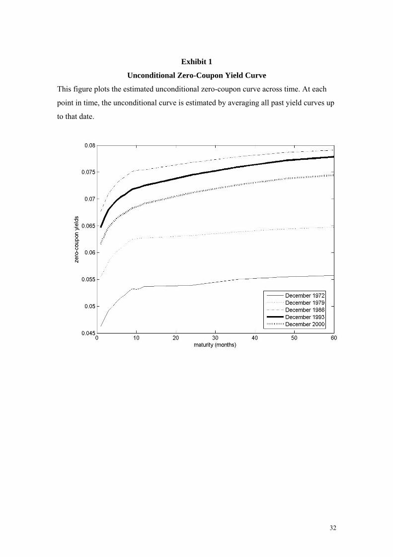
Exhibit 1

Unconditional Zero-Coupon Yield Curve

This figure plots the estimated unconditional zero-coupon curve across time. At each

point in time, the unconditional curve is estimated by averaging all past yield curves up

to that date.

32

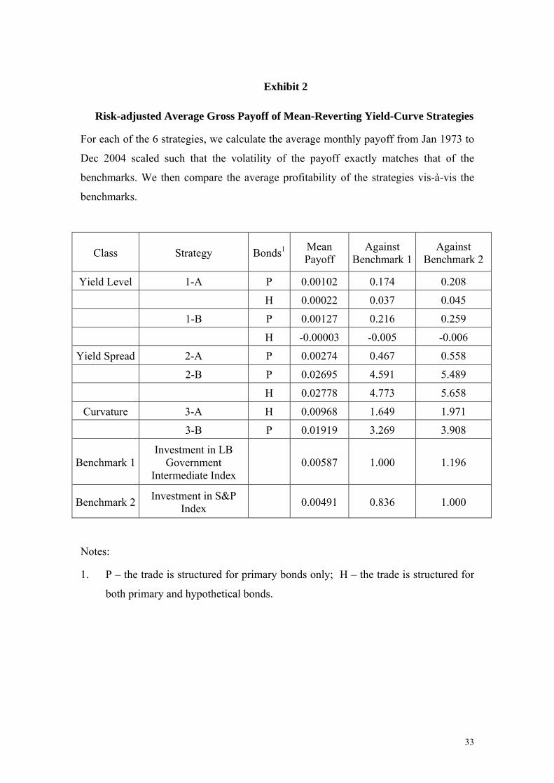
Exhibit 2

Risk-adjusted Average Gross Payoff of Mean-Reverting Yield-Curve Strategies

For each of the 6 strategies, we calculate the average monthly payoff from Jan 1973 to

Dec 2004 scaled such that the volatility of the payoff exactly matches that of the

benchmarks. We then compare the average profitability of the strategies vis-à-vis the

benchmarks.

Class Strategy Bonds1 Mean Payoff

Against Benchmark 1

Against Benchmark 2

Yield Level 1-A P 0.00102 0.174 0.208

H 0.00022 0.037 0.045

1-B P 0.00127 0.216 0.259

H -0.00003 -0.005 -0.006

Yield Spread 2-A P 0.00274 0.467 0.558

2-B P 0.02695 4.591 5.489

H 0.02778 4.773 5.658

Curvature 3-A H 0.00968 1.649 1.971

3-B P 0.01919 3.269 3.908

Benchmark 1 Investment in LB

Government Intermediate Index

0.00587 1.000 1.196

Benchmark 2 Investment in S&P Index 0.00491 0.836 1.000

Notes:

1. P – the trade is structured for primary bonds only; H – the trade is structured for

both primary and hypothetical bonds.

33

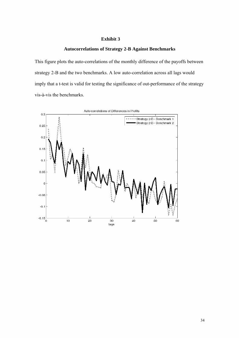
Exhibit 3

Autocorrelations of Strategy 2-B Against Benchmarks

This figure plots the auto-correlations of the monthly difference of the payoffs between

strategy 2-B and the two benchmarks. A low auto-correlation across all lags would

imply that a t-test is valid for testing the significance of out-performance of the strategy

vis-à-vis the benchmarks.

34

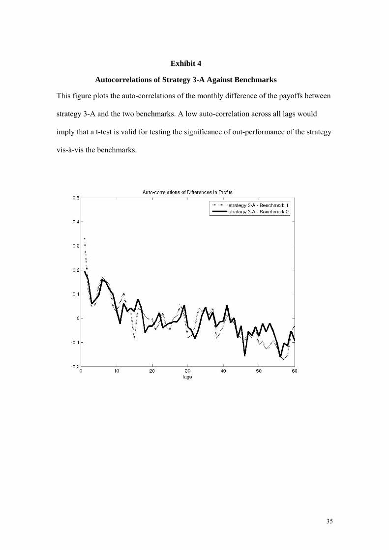
Exhibit 4

Autocorrelations of Strategy 3-A Against Benchmarks

This figure plots the auto-correlations of the monthly difference of the payoffs between

strategy 3-A and the two benchmarks. A low auto-correlation across all lags would

imply that a t-test is valid for testing the significance of out-performance of the strategy

vis-à-vis the benchmarks.

35

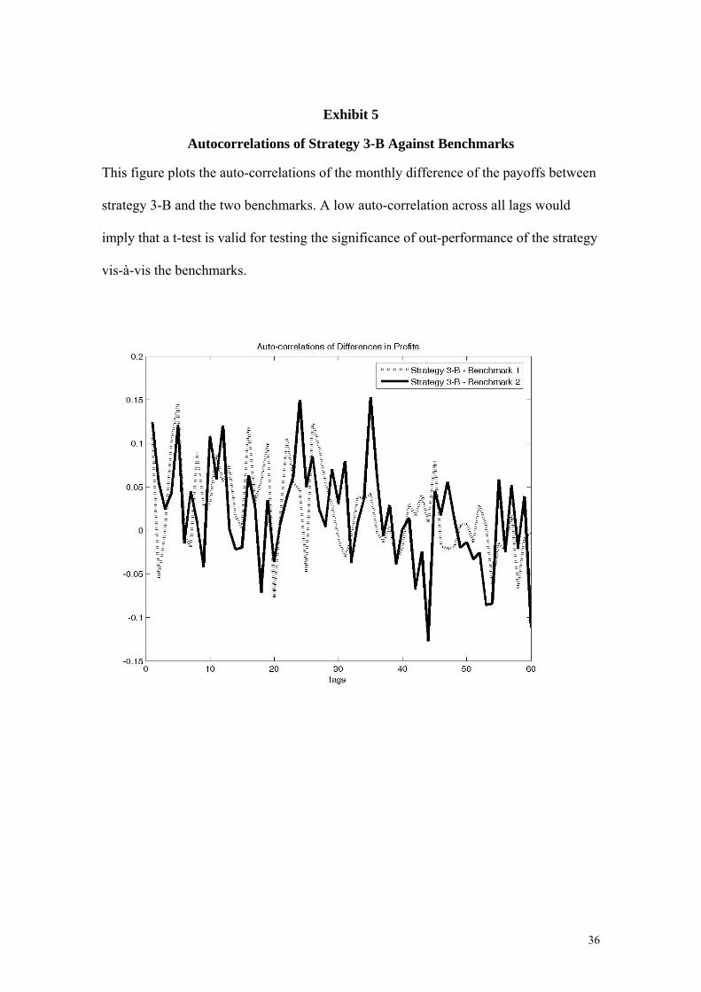
Exhibit 5

Autocorrelations of Strategy 3-B Against Benchmarks

This figure plots the auto-correlations of the monthly difference of the payoffs between

strategy 3-B and the two benchmarks. A low auto-correlation across all lags would

imply that a t-test is valid for testing the significance of out-performance of the strategy

vis-à-vis the benchmarks.

36

Exhibit 6

Significance Tests of Excess Payoffs of Strategies with respect to Benchmarks

For the 3 most profitable strategies (2-B, 3-A and 3-B), we perform significance test on

their profitability. We test whether the average profits are significantly more than zero,

as well as whether the profits are significantly more than the benchmarks. We use two

types of test—the more powerful (but potentially less valid) t-test, as well as the

Newey-West test.

Strategy

2-B1 3-A 3-B

Mean Payoff 0.02695 0.00968 0.01919

Statistic p-value Statistic p-value Statistic p-value

vs zero profits 11.885 0.000 4.270 0.000 8.464 0.000

vs Benchmark 1 6.659 0.000 1.076 0.282 4.300 0.000 t-test

vs Benchmark 2 7.076 0.000 1.523 0.129 4.447 0.000

vs zero profits 5.061 0.000 2.348 0.019 4.347 0.000

vs Benchmark 1 3.116 0.002 0.526 0.633 2.479 0.013 N-W

test vs Benchmark 2 3.432 0.001 0.357 0.920 2.654 0.008

Note:

1. We report the significance tests for the trade structured with primary bonds only.

The results of the significance tests for strategy 2-B using the trade structured for

both primary and hypothetical bonds are essentially identical.

2. We assume that the benchmarks are traded with zero transaction cost.

37

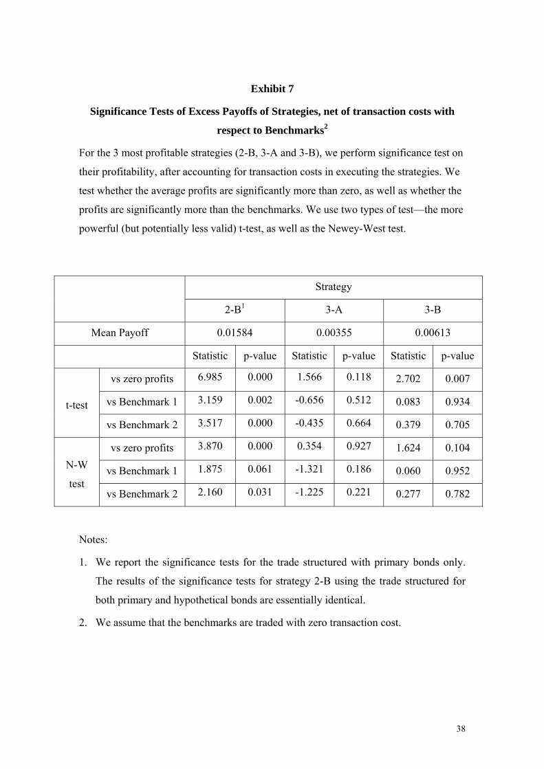
Exhibit 7

Significance Tests of Excess Payoffs of Strategies, net of transaction costs with

respect to Benchmarks2

For the 3 most profitable strategies (2-B, 3-A and 3-B), we perform significance test on

their profitability, after accounting for transaction costs in executing the strategies. We

test whether the average profits are significantly more than zero, as well as whether the

profits are significantly more than the benchmarks. We use two types of test—the more

powerful (but potentially less valid) t-test, as well as the Newey-West test.

Strategy

2-B1 3-A 3-B

Mean Payoff 0.01584 0.00355 0.00613

Statistic p-value Statistic p-value Statistic p-value

vs zero profits 6.985 0.000 1.566 0.118 2.702 0.007

vs Benchmark 1 3.159 0.002 -0.656 0.512 0.083 0.934 t-test

vs Benchmark 2 3.517 0.000 -0.435 0.664 0.379 0.705

vs zero profits 3.870 0.000 0.354 0.927 1.624 0.104

vs Benchmark 1 1.875 0.061 -1.321 0.186 0.060 0.952 N-W

test vs Benchmark 2 2.160 0.031 -1.225 0.221 0.277 0.782

Notes:

1. We report the significance tests for the trade structured with primary bonds only.

The results of the significance tests for strategy 2-B using the trade structured for

both primary and hypothetical bonds are essentially identical.

2. We assume that the benchmarks are traded with zero transaction cost.

38

Exhibit 8

Test of Value-Added of Mean-Reverting Strategies (net of transaction costs) to a

Buy-and-Hold Investment in the S&P Index (Jensen’s alpha)

This table lists the usefulness of each strategy when it is added to one that buys-

and-holds the S&P index (Foster and Stine [2003]). Excess returns of the strategy

(Y) are regressed on the excess return of the S&P index (X). If the t-stat of the

intercept is significantly positive, this will imply that the particular strategy can add

value to a simple buy-and-hold S&P strategy.

Strategy

2-B 3-A 3-B

t-stat p-value t-stat p-value t-stat p-value

alpha 6.816 0.000 1.449 0.148 2.685 0.008

39

Exhibit 9

Contribution of Different Trades to the Payoff of Strategy 2-B (Primary Bonds)

This figure plots the contribution of various trade segments of strategy 2-B to the overall

profitability of the strategy. The overall profitability of the strategy is not dominated by any

particular segment of the yield curve. Rather, almost all of the segments (with the exception of 2

segments) contribute substantially to the profitability.

-0.05

0

0.05

0.1

0.15

0.2

0.25

1 2 3 4 5 6 7 8 9 10 11 12 13 14

Trade Segment

Prop

ortio

n of

Tot

al P

rofit

Trade segments of strategy 2-B: Yield spread mean-reversion trade, on the 1-month forward curve

1. 1-2 month spread 2. 2-3 month spread 3. 3-4 month spread 4. 4-5 month spread 5. 5-6 month spread 6. 6-7 month spread 7. 7-8 month spread 8. 8-9 month spread 9. 9-10 month spread 10. 10-11 month spread 11. 11-23 month spread 12. 23-35 month spread 13. 35-47 month spread 14. 47-59 month spread

40

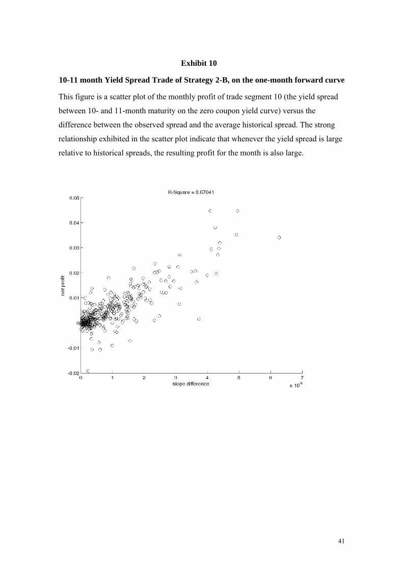
Exhibit 10

10-11 month Yield Spread Trade of Strategy 2-B, on the one-month forward curve

This figure is a scatter plot of the monthly profit of trade segment 10 (the yield spread

between 10- and 11-month maturity on the zero coupon yield curve) versus the

difference between the observed spread and the average historical spread. The strong

relationship exhibited in the scatter plot indicate that whenever the yield spread is large

relative to historical spreads, the resulting profit for the month is also large.

41

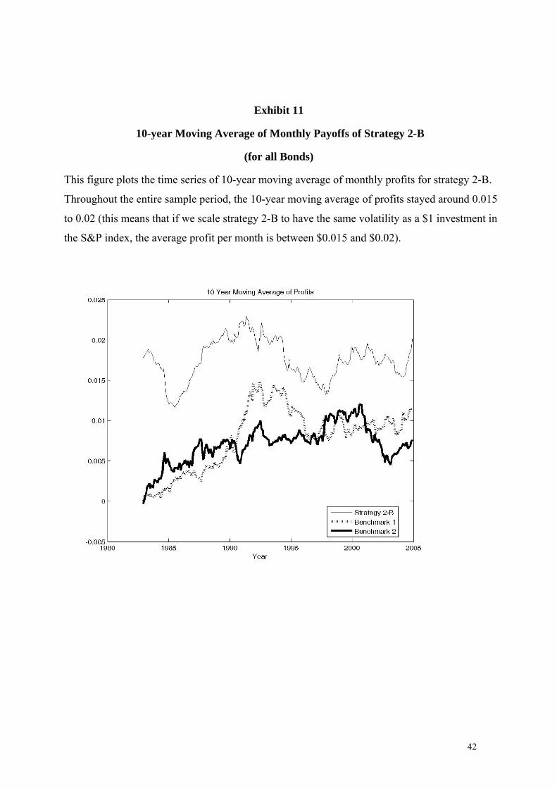
Exhibit 11

10-year Moving Average of Monthly Payoffs of Strategy 2-B

(for all Bonds)

This figure plots the time series of 10-year moving average of monthly profits for strategy 2-B.

Throughout the entire sample period, the 10-year moving average of profits stayed around 0.015

to 0.02 (this means that if we scale strategy 2-B to have the same volatility as a $1 investment in

the S&P index, the average profit per month is between $0.015 and $0.02).

42