Laurea Magistrale

in Ingegneria Matematica

Progetto per il corso di

Programmazione Avanzata per il Calcolo Scientico

Professor Luca Formaggia

Riduzione gerarchica di modelloper problemi ADR su domini a sezione circlare

Progetto di:

Guzzetti Soa

Matr. 782674

Lupo Pasini Massimiliano

Matr. 782283

Anno Accademico 20122013

Contents

1 Description of the method 3

2 Educated Basis 8

3 Implementation 11

3.1 BasisAbstract . . . . . . . . . . . . . . . . . . . . . . . . . . . . . . . . . . . . . . . . 11

4 ModalSpace 16

5 HiModAssembler 21

6 Numerical results 24

References33

1

Introduction

A lot of engineering topics are solved modeling them with partial dierential problems. Anyway itusually happens that the complexity of the phenomenon to be analyzed translates likewise into avery intricate mathematical modeling of the problem to be solved too. Thus it is strictly importantto develop proper algorithms that enable us to achieve a reliable solution with a managed expensein terms of computational cost and resources that have to be spent to get them. The complexity ofthe problem might be associated with the shape of the domain where the event is set rather thanthe considerably high number of coecients to be considered in the equations that characterizethe model. In the worst cases these two aspects raise at the same time. Today a lot of problemsconcerning scientic matters and engineering can't be solved due to the shortage of proper devicesto be able to sustain the amount of computation which is necessary. It is strictly associated with theevolution of numerical analysis which, in the recent years, had the goal to solve analytical problemsthat are characterized by a huge number of variables, pushing forward the frontiers created bycalculators' limited ability.

Indeed this work takes place in the eld of model reduction algorithms which nowadays are usedvery widely to solve high dimensional partial dierential problems in order to nd a good compro-mise between solution error and computational costs which are required by the implementation ofthe method itself.

Nowadays there are dierent methods which try to address the problem induced by curse ofdimensionality. One of them is the POD (Proper Orthogonal Decomposition) whose aim is torepresent high-dimensional problems in a reduced space so to express the solution of the problemas a linear combination of base functions that are properly selected by the algorithm.

Another way of proceeding to reduce the complexity of the problems consists in adopting dier-ent kind of discretization along dierent dimensions of the domain. That's the case of HierarchicalModel Reduction (Hi-Mod). As it is shown in [EPV08], [PEV], [PEV10] and [PZ13] the spirit ofthis method is to detect if there is one direction which is more important than others to describethe phenomenon. If so, then along this way a Finite Element discretization is applied, instead alongall the others the discretization is done by pseudo-spectral methods. The result is a linear systemwhose stiness matrix is much easier to treat from a numerical point of view rather than usingFinite Elements along all the dimensions of the domain.

The goal of our work is to use Hierarchical Model Reduction to solve 3D partial dierentialproblems that are dened on a domain whose geometry is not a parallelepiped, but for instancea cylinder with a circular base. Furthermore we will consider dierent boundary conditions to becoupled to the partial dierential equation to fully determine the problem to be solved.

2

1 Description of the method

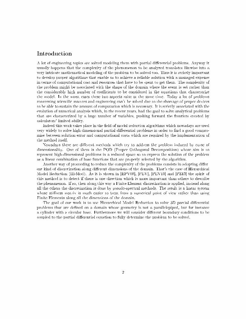
Let us consider for example an advection-diusion-reaction problem set on a cylindric domain:−µ∆u+ b · ∇u+ σu = f in Ω

u = uin on Γin∂u∂x = 0 on Γout

u = 0 on Γside

Ω = (x, ρ, θ) : 0 < x < a, 0 < ρ < R, 0 < ρ < 2π,Γin ∩ Γout ∩ Γside = ∅, Γin ∪ Γout ∪ Γside = ∂Ω.

(1)

Figure 1: Tubular domain

The coecients of (1) are set so that well-posedness of its variational form is guaranteed byLax-Milgram Theorem.

To develop the problem in the weak form it is necessary to introduce a proper funcional setting.For this we appeal to the Sobolev Space:

H10,Γ(Ω) = v ∈ H1(Ω) : v |Γ= 0

where ∂Ω is the boundary of the set Ω and H1(Ω) is dened as:

H1(Ω) = v ∈ L2(Ω) : ∇v ∈ [L2(Ω)]d.

∇(·) denotes the gradient operator and d is the number of dimensions of Rd so that Ω ⊂ Rd. Inour case d = 3.

Thanks to the properties of Banach space L2(Ω) which is also an Hilbert one, it descends thatH1(Ω) is an Hilbert space too, as all its subsets. Thus it is possible to introduce the dual toH1(Ω) whose symbol is [H1(Ω)]∗ and for sake of simplicity we will refer to it with the abbreviatedrepresentation H−1(Ω).

We use the following convention:

3

• ΓD=portion of frontier ∂Ω with Dirichlet boundary conditions (thus Γin ⊂ ΓD)

• ΓN=portion of frontier ∂Ω with Neumann boundary conditions

• ΓR=portion of frontier ∂Ω with Robin boundary conditions

The weak form of the problem descends as follows:nd u ∈ H1

0,ΓD(Ω) so that

∫Ω

(−µ∆u+ b · ∇u+ σu− f)vdω = 0 ∀v ∈ H10,ΓD

(Ω). (2)

Integrating by parts we obtain:∫Ω

[µ∇u · ∇v + (b · ∇u)v + σuv

]dω −

∫∂Ω\ΓD

µ∂u

∂nv =

∫Ω

fvdω ∀v ∈ H10,ΓD

(Ω). (3)

Introducing function g ∈ H1(Ω) dened as follows:

g |ΓD= u |ΓD

,

we can modify the previuos weak form so that: u = u+ g∫Ω

[µ∇u·∇v+(b·∇u)v+σuv

]dω−

∫∂Ω\ΓD

µ∂u

∂nv = −

∫Ω

[µ∇g·∇v+(b·∇g)v+σgv

]dω+

∫Ω

fvdω ∀v ∈ H10,ΓD

(Ω).

(4)The last form of the variational problem enables us to use Lax-Milgram theorem. In fact

introducing a bilinear form:a(·, ·) : H1

0,ΓD×H1

0,ΓD→ R

and a functional F ∈ [H10,ΓD

]∗:F : H1

0,ΓD→ R

we can dene them as follows:

a(u, v) =

∫Ω

[µ∇u · ∇v + (b · ∇u)v + σuv

]dω −

∫∂Ω\ΓD

µ∂u

∂nv

F (v) =

∫Ω

fvdω

Therefore the variational form of the problem turns into:

nd u ∈ H10,ΓD

so that a(u, v) = F (v) ∀v ∈ H10,ΓD

. (5)

Bilinear form a(·, ·) and and functional F (·) satises all the hypothesis that are required by Lax-Milgram theorem, so one and only one solution to (5) is guaranteed.

For our purposes domain Ω will be an open right circular cylinder with constants transversalsections which has the property to be dened as a tensor product:

Ω = [a, b]× ΣR,

4

[a, b] is the range for variable x along the horizontal direction and ΣR is a generic circular section.For sake of simplicity we will refer to the radius of circular section with R and to the length of thehorizontal dimension of the cylinder with L.

If R L, then phenomenon is characterized by a privileged direction (mainstream) which isdetected by variable x, instead what happens in the transversal section ΣR can be synthetized inproper coecients in view of a model reduction.

In fact the particular structure of the domain gives us the chance to solve the partial dierentialproblem using a simplied method that cut down the complexity of the algorithm to be adopted.

In order to do this we introduce an orthogonal base ϕii∈N for H1(Σ) that needs to be or-thonormal respect to L2(Σ) (weighted) scalar product. Thus solution to 5 can be expressed in thefollowing way:

u(x, ρ, θ) =

∞∑i=0

ui(x)ϕi(ρ, θ).

We can notice that the tensorial structure of the domain translates into a tensorial structure ofthe solution itself. This way of proceeding is at the basis of our discretization method. In detail wewill use dierent discretizing approaches along the mainstream and in the transversal section.

As concerns the vertical ber the approximation consists in truncating the number of Fouriercoecients that are used to build the value of the solution along the transversal section:

u(x, ρ, θ) ≈m∑i=0

ui(x)ϕi(ρ, θ), m ∈ N.

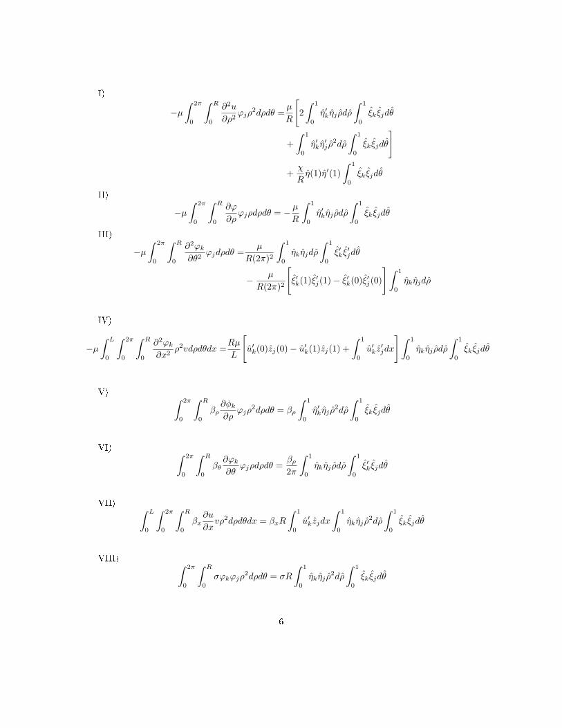
Setting 5 in this functional framework and integrating along the transversal section of the domainwe introduce a set of proper coecients for the unidimensional equation along the mainstream. Todo this we multiplied both the member of the equation with ρ in order to neglect the singularity ofthe elliptic operator in cylindric reference system for ρ = 0.

− µ∫ L

0

∫ 2π

0

∫ R

0

(∂2u

∂ρ2+

1

ρ

∂u

∂ρ+

1

ρ2

∂2u

∂θ2+∂2u

∂x2

)vρ2dρdθdx

+

∫ L

0

∫ 2π

0

∫ R

0

(βx∂u

∂x+ βρ

∂u

∂ρ+ βθ

1

ρ

∂u

∂θ

)vρ2dρdθdx

+

∫ L

0

∫ 2π

0

∫ R

0

σuvρ2dρdθdx =

∫ L

0

∫ 2π

0

∫ R

0

fvρ2dρdθdx

(6)

Applying variable separation we obtain:

u(x, ρ, θ) =

M∑k=1

uk(x)ϕk(ρ, θ) (7)

ϕk(ρ, θ) =1

R√

2πηk(ρ)ξ(θ) (8)

and dening zj as the j-th Finite Element basis function the integrals above can be written asthe following:

5

I)

−µ∫ 2π

0

∫ R

0

∂2u

∂ρ2ϕjρ

2dρdθ =µ

R

[2

∫ 1

0

η′kηj ρdρ

∫ 1

0

ξk ξjdθ

+

∫ 1

0

η′kη′j ρ

2dρ

∫ 1

0

ξk ξjdθ

]

+χ

Rη(1)η′(1)

∫ 1

0

ξk ξjdθ

II)

−µ∫ 2π

0

∫ R

0

∂ϕ

∂ρϕjρdρdθ = − µ

R

∫ 1

0

η′kηj ρdρ

∫ 1

0

ξk ξjdθ

III)

−µ∫ 2π

0

∫ R

0

∂2ϕk∂θ2

ϕjdρdθ =µ

R(2π)2

∫ 1

0

ηkηjdρ

∫ 1

0

ξ′k ξ′jdθ

− µ

R(2π)2

[ξ′k(1)ξ′j(1)− ξ′k(0)ξ′j(0)

]∫ 1

0

ηkηjdρ

IV)

−µ∫ L

0

∫ 2π

0

∫ R

0

∂2ϕk∂x2

ρ2vdρdθdx =Rµ

L

[u′k(0)zj(0)− u′k(1)zj(1) +

∫ 1

0

u′kz′jdx

]∫ 1

0

ηkηj ρdρ

∫ 1

0

ξk ξjdθ

V) ∫ 2π

0

∫ R

0

βρ∂φk∂ρ

ϕjρ2dρdθ = βρ

∫ 1

0

η′kηj ρ2dρ

∫ 1

0

ξk ξjdθ

VI) ∫ 2π

0

∫ R

0

βθ∂ϕk∂θ

ϕjρdρdθ =βρ2π

∫ 1

0

ηkηj ρdρ

∫ 1

0

ξ′k ξjdθ

VII) ∫ L

0

∫ 2π

0

∫ R

0

βx∂u

∂xvρ2dρdθdx = βxR

∫ 1

0

u′kzjdx

∫ 1

0

ηkηj ρ2dρ

∫ 1

0

ξk ξjdθ

VIII) ∫ 2π

0

∫ R

0

σϕkϕjρ2dρdθ = σR

∫ 1

0

ηkηj ρ2dρ

∫ 1

0

ξk ξjdθ

6

This enables us to read a set of one-dimensional ADR problems, one for each couple (j, k) ofmodal functions.

In the cases that we will consider, the coecients of the equation are constant and this makespossible to additionally apply separation of variables upon (ρ, θ).

7

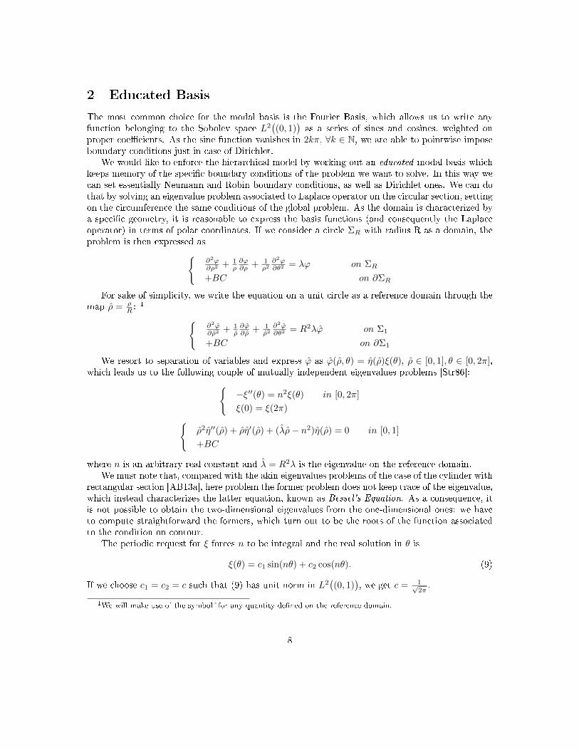
2 Educated Basis

The most common choice for the modal basis is the Fourier Basis, which allows us to write anyfunction belonging to the Sobolev space L2

((0, 1)

)as a series of sines and cosines, weighted on

proper coecients. As the sine function vanishes in 2kπ, ∀k ∈ N, we are able to pointwise imposeboundary conditions just in case of Dirichlet.

We would like to enforce the hierarchical model by working out an educated modal basis whichkeeps memory of the specic boundary conditions of the problem we want to solve. In this way wecan set essentially Neumann and Robin boundary conditions, as well as Dirichlet ones. We can dothat by solving an eigenvalue problem associated to Laplace operator on the circular section, settingon the circumference the same conditions of the global problem. As the domain is characterized bya specic geometry, it is reasonable to express the basis functions (and consequently the Laplaceoperator) in terms of polar coordinates. If we consider a circle ΣR with radius R as a domain, theproblem is then expressed as

∂2ϕ∂ρ2 + 1

ρ∂ϕ∂ρ + 1

ρ2∂2ϕ∂θ2 = λϕ on ΣR

+BC on ∂ΣR

For sake of simplicity, we write the equation on a unit circle as a reference domain through themap ρ = ρ

R :1

∂2ϕ∂ρ2 + 1

ρ∂ϕ∂ρ + 1

ρ2∂2ϕ∂θ2 = R2λϕ on Σ1

+BC on ∂Σ1

We resort to separation of variables and express ϕ as ϕ(ρ, θ) = η(ρ)ξ(θ), ρ ∈ [0, 1], θ ∈ [0, 2π],which leads us to the following couple of mutually independent eigenvalues problems [Str86]:

−ξ′′(θ) = n2ξ(θ) in [0, 2π]

ξ(0) = ξ(2π)ρ2η′′(ρ) + ρη′(ρ) + (λρ− n2)η(ρ) = 0 in [0, 1]

+BC

where n is an arbitrary real constant and λ = R2λ is the eigenvalue on the reference domain.We must note that, compared with the akin eigenvalues problems of the case of the cylinder with

rectangular section [AB13a], here problem the former problem does not keep trace of the eigenvalue,which instead characterizes the latter equation, known as Bessel's Equation. As a consequence, itis not possible to obtain the two-dimensional eigenvalues from the one-dimensional ones: we haveto compute straightforward the formers, which turn out to be the roots of the function associatedto the condition on contour.

The periodic request for ξ forces n to be integral and the real solution in θ is

ξ(θ) = c1 sin(nθ) + c2 cos(nθ). (9)

If we choose c1 = c2 = c such that (9) has unit norm in L2((0, 1)

), we get c = 1√

2π.

1We will make use of the symbolˆfor any quantity dened on the reference domain.

8

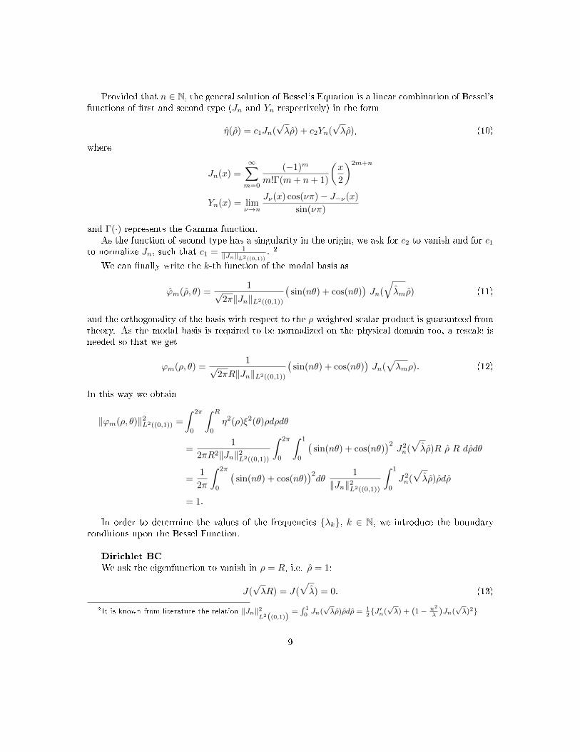
Provided that n ∈ N, the general solution of Bessel's Equation is a linear combination of Bessel'sfunctions of rst and second type (Jn and Yn respectively) in the form

η(ρ) = c1Jn(√λρ) + c2Yn(

√λρ), (10)

where

Jn(x) =

∞∑m=0

(−1)m

m!Γ(m+ n+ 1)

(x

2

)2m+n

Yn(x) = limν→n

Jν(x) cos(νπ)− J−ν(x)

sin(νπ)

and Γ(·) represents the Gamma function.As the function of second type has a singularity in the origin, we ask for c2 to vanish and for c1

to normalize Jn, such that c1 = 1‖Jn‖L2((0,1))

. 2

We can nally write the k-th function of the modal basis as

ϕm(ρ, θ) =1√

2π‖Jn‖L2((0,1))

(sin(nθ) + cos(nθ)

)Jn(

√λmρ) (11)

and the orthogonality of the basis with respect to the ρ-weighted scalar product is guaranteed fromtheory. As the modal basis is required to be normalized on the physical domain too, a rescale isneeded so that we get

ϕm(ρ, θ) =1√

2πR‖Jn‖L2((0,1))

(sin(nθ) + cos(nθ)

)Jn(√λmρ). (12)

In this way we obtain

‖ϕm(ρ, θ)‖2L2((0,1)) =

∫ 2π

0

∫ R

0

η2(ρ)ξ2(θ)ρdρdθ

=1

2πR2‖Jn‖2L2((0,1))

∫ 2π

0

∫ 1

0

(sin(nθ) + cos(nθ)

)2J2n(√λρ)R ρ R dρdθ

=1

2π

∫ 2π

0

(sin(nθ) + cos(nθ)

)2dθ

1

‖Jn‖2L2((0,1))

∫ 1

0

J2n(√λρ)ρdρ

= 1.

In order to determine the values of the frequencies λk, k ∈ N, we introduce the boundaryconditions upon the Bessel Function.

Dirichlet BC

We ask the eigenfunction to vanish in ρ = R, i.e. ρ = 1:

J(√λR) = J(

√λ) = 0. (13)

2It is known from literature the relation ‖Jn‖2L2((0,1)

) =∫ 10 Jn(

√λρ)ρdρ = 1

2J ′n(√λ) +

(1− n2

λ

)Jn(√λ)2

9

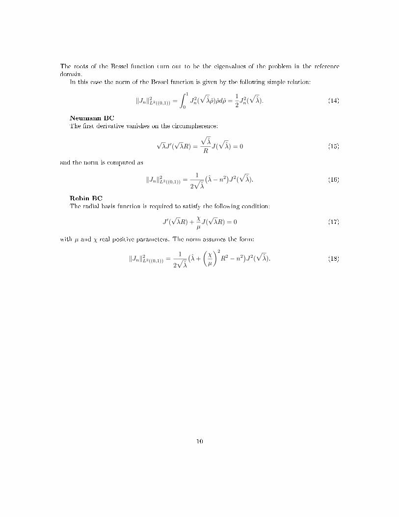
The roots of the Bessel function turn out to be the eigenvalues of the problem in the referencedomain.

In this case the norm of the Bessel function is given by the following simple relation:

‖Jn‖2L2((0,1)) =

∫ 1

0

J2n(√λρ)ρdρ =

1

2J2n(√λ). (14)

Neumann BC

The rst derivative vanishes on the circumpherence:

√λJ ′(√λR) =

√λ

RJ(√λ) = 0 (15)

and the norm is computed as

‖Jn‖2L2((0,1)) =1

2√λ

(λ− n2

)J2(√λ). (16)

Robin BC

The radial basis function is required to satisfy the following condition:

J ′(√λR) +

χ

µJ(√λR) = 0 (17)

with µ and χ real positive parameters. The norm assumes the form:

‖Jn‖2L2((0,1)) =1

2√λ

(λ+

(χ

µ

)2

R2 − n2)J2(√λ). (18)

10

3 Implementation

The code has been developed in LifeV and is located in branch 20131017_HiMod2. We made useof cmake for the compilation and git for managing the scripts. Vectors and matrices have beenhandled with specic tools in LifeV, which are based on Trilinos, while the assembling of thesub-problems has been achieved through Expression Templates (ETA). The code is serial, in fact aparallel execution would need proper structures able to deal with the pattern of the system matrix.

The evaluation of the Bessel functions is already implemented in the Navier_Stokes package,while the algorithm to nd the roots of the function itself and its derivatives has been developedon the base of a fortran code by Jin and Zhang [ZJ96].

The domain of the computation is a cylinder of length Lx with circular section of radius R.We want to solve a steady ADR problem with generic Dirichlet inow conditions and homogeneousNeumann conditions in outow. We assume homogeneous conditions on the lateral wall and thatthe coecients of the problem are constant. Moreover we suppose that it is possible to treat thetwo-dimensional problem on the section through the splitting of the radial and angular coordinates.

Our code is an extension of the branch named 20130507_HiMod, which solves the same problemon a cylinder with rectangular section. The geometric nature of the domain induces us to use acylindric reference system, which implies a radical change in the sturcture of the problem. As wehave seen before, in fact, the information about the two-dimensional problem is contained in onlyone 1D problem as a whole, while the other one determines the periodicity of the solution.

We tried to keep the pre-existent code untouched as much as possible and to keep a similarframework in the implementation of the new classes. For this purpose we made large use of templateclasses and inheritance.

The code is organized in three dierent levels which refer to the progressive dimension of theproblem we want to solve. BasisAbstract deals with the one-dimensional problem associated tothe search of the main frequences of the problem. The former Basis1DAbstract and the latestBasis2DAbstract inherit from it. They both handle boundary conditions.

ModalSpaceRectangular and ModalSpaceCircular, whose father-class is ModalSpaceAbstract, as-semble the two one-dimensional problems into the one dened on the section of the cylinder. Theybuild the real modal basis by choosing the proper frequences among those computed by a Basis1Dor a Basis2D, compute the Fourier coecients and the numeric integrals for the weak formulationof the problem.

The nal link which leads to the three-dimensional problem is performed by HiModAssembler,which is a template class such that the shape of the section is given as a parameter. It builds thematrix and the known term of the equation.

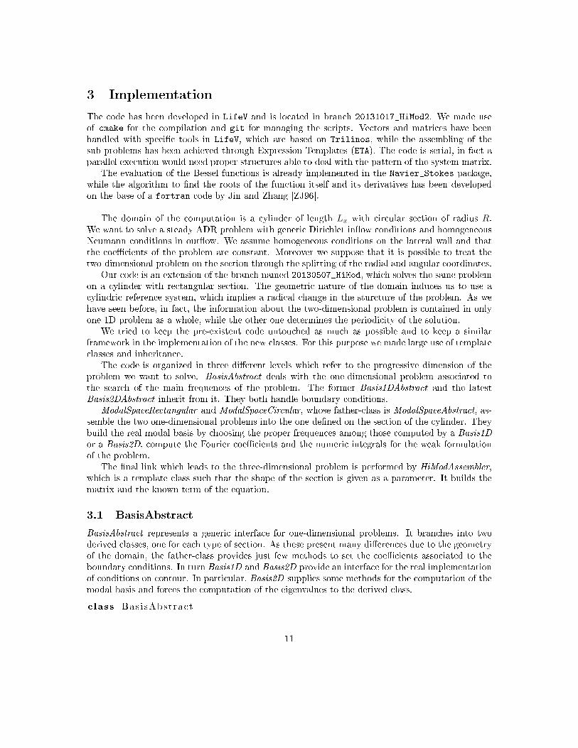
3.1 BasisAbstract

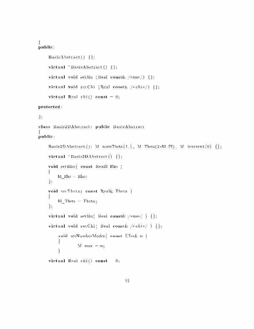
BasisAbstract represents a generic interface for one-dimensional problems. It branches into twoderived classes, one for each type of section. As these present many dierences due to the geometryof the domain, the father-class provides just few methods to set the coecients associated to theboundary conditions. In turn Basis1D and Basis2D provide an interface for the real implementationof conditions on contour. In particular, Basis2D supplies some methods for the computation of themodal basis and forces the computation of the eigenvalues to the derived class.

class Bas i sAbstract

11

public :

Bas i sAbstract ( ) ;

virtual ~Bas i sAbstract ( ) ;

virtual void setMu ( Real const& /∗mu∗/ ) ;

virtual void setChi ( Real const& /∗ ch i ∗/ ) ;

virtual Real ch i ( ) const = 0 ;

protected :

;

class Basis2DAbstract : public Bas i sAbstractpublic :

Basis2DAbstract ( ) : M_normTheta ( 1 . ) , M_Theta(2∗M_PI) , M_icurrent (0 ) ;

virtual ~Basis2DAbstract ( ) ;

void setRho ( const Real& Rho )

M_Rho = Rho ; ;

void setTheta ( const Real& Theta )

M_Theta = Theta ; ;

virtual void setMu ( Real const& /∗mu∗/ ) ;

virtual void setChi ( Real const& /∗ ch i ∗/ ) ;

void setNumberModes ( const UInt& m )

M_mtot = m;

virtual Real ch i ( ) const = 0 ;

12

virtual EigenContainer e igenValues ( ) const

return M_eigenvalues ;

;

virtual void computeEigenvalues ( ) = 0 ;

void

eva lua t eBas i s ( MBMatrix_type& phirho ,MBMatrix_type& dphirho ,MBMatrix_type& phitheta ,MBMatrix_type& dphitheta ,const EigenContainer& e igenva lue s ,const QuadratureRule∗ quadrulerho ,const QuadratureRule∗ quadru le theta ) const ;

Realeva lS ing l ePo in t ( const Real& eigen , const UInt index , const

MBVector_type& p ) const ;

protected :

Real M_Rho;Real M_Theta ;UInt M_icurrent ;UInt M_mtot ;EigenContainer M_eigenvalues ;Real M_normTheta ;MBVector_type M_normRJ;

;

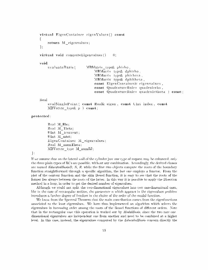
If we assume that on the lateral wall of the cylinder just one type of request may be enhanced, onlythe three plain types of BCs are possible, without any combination. Accordingly, the derived classesare named EducatedBasisD, N, R. while the rst two objects compute the roots of the boundaryfunction straightforward through a specic algorithm, the last one employs a functor. From theplot of the contour function and the akin Bessel function, it is easy to see that the roots of theformer lies always between the roots of the latter. In this way it is possible to apply the Bisectionmethod in a loop, in order to get the desired number of eigenvalues.

Although we could not split the two-dimensional eigenvalues into two one-dimensional ones,like in the case of rectangular section, the parameter n which appears in the eigenvalues problemintroduces a further degree of freedom in the choice of the order of the modal function.

We know from the Spectral Theorem that the main contribution comes from the eigenfunctionsassociated to the least eigenvalues. We have thus implemented an algorithm which selects theeigenvalues in increasing order among the roots of the Bessel functions of dierent orders. Notethat in the rectangular case this operation is worked out by ModalBasis, since the two rare one-dimensional eigenvalues are independent one from another and need to be combined at a higherlevel. In this case, instead, the eigenvalues computed by the EducatedBasis concern directly the

13

problem on the section, so it is reasonable to compute the entire basis here.The eigenvalues are computed by computeEigenvalues in the following way: the least one is

the rst root associated to the Bessel function of order zero. According to the nature of thesefunctions, at each stage of the search the next bigger eigenvalue may be the next root of thefunction of the same order, or the next root of the function of higher order. At each step we insertthese two candidates in a ordered set in such a way that the rst element of the set is the least ofall the candidates inserted so far. The abstract class then provides the methods evaluateBasisand evalSinglePoint to evaluate the modal basis on quadrature points and in any point for anyboundary condition, since the information is condensed into the eigenvalues.

14

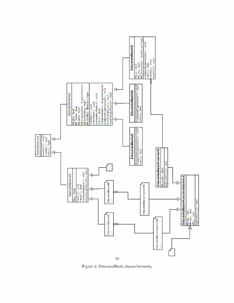
Figure 2: EducatedBasis classes hierarchy

15

4 ModalSpace

ModalSpaceAbstract provides the methods to compute the lumped coecients which take into ac-count all the information coming from the section when solving the one-dimensional problem. Itcomputes also Fourier coecients, useful in the assembling of the problem and in the postprocessingof the solution.

class ModalSpaceAbstract

public :ModalSpaceAbstract ( UInt m) : M_mtot(m) ;

virtual ~ModalSpaceAbstract ( ) ;

virtual void eva lua t eBas i s ()=0;

virtual std : : vector<Real> f o u r i e r C o e f f i c i e n t s ( const function_Type& g )const = 0 ;

virtual Real f our i e rCoe f fPo in tWise ( const Real& x , const function_Type&f , const UInt& k) const = 0 ;

virtual Real compute_R11 ( const UInt& j , const UInt& k ,const function_Type& mu, const Real& x) const = 0 ;

virtual Real compute_R10 ( const UInt& j , const UInt& k ,const function_Type& beta , const Real& x) const =

0 ;

virtual Real compute_R00 ( const UInt& j , const UInt& k ,const function_Type& mu, const function_Type&

beta , const function_Type& sigma , const Real& x) const = 0 ;

virtual void showMe ( ) const = 0 ;

UInt mtot ( ) const

protected :

virtual void e i g en sProv ide r ()=0;

UInt M_mtot ;

;

ModalSpaceRectangular andModalSpaceCircular derive from the abstract class. Dierently fromthe case of the rectangle, in case of the circle the two-dimensional eigenvalues are computed directly

16

by the proper EducatedBasis, so the method eigensProvider only recalls the eigenvalues from thebasis it points to and assign them to those of the modal basis. In the same way, evaluateBasisextracts the values of the modal functions previously computed by the proper educated basis,instantiated through the method addSliceBC.

The other members of the class are mainly functions which carry out the numeric computationof the integrals used do build the lumped parameters in polar coordinates. Note that the equationhas a singularity in ρ = 0, so we multiply both the members for ρ. In this way when we integratethe weight simplies the singularity. The integrals are computed as described here:

• compute1_PhiPhi∫ 2π

0

∫ R0ϕiϕkρdρdθ

• compute2_PhiPhi∫ 2π

0

∫ R0ϕiϕkρ

2dρdθ

• compute1_DrhoPhiPhi∫ 2π

0

∫ R0

∂ϕi

∂ρ ϕkρdρdθ

• compute2_DrhoPhiPhi∫ 2π

0

∫ R0

∂ϕi

∂ρ ϕkρ2dρdθ

• compute1_DrhoPhiDrhoPhi∫ 2π

0

∫ R0

∂ϕi

∂ρ∂ϕk

∂ρ ρdρdθ

• compute2_DrhoPhiDrhoPhi∫ 2π

0

∫ R0

∂ϕi

∂ρ∂ϕk

∂ρ ρ2dρdθ

• compute1_DthetaPhiPhi∫ 2π

0

∫ R0

∂ϕi

∂θ ϕkρdρdθ

• compute0_DthetaPhiDthetaPhi∫ 2π

0

∫ R0

∂ϕi

∂θ∂ϕk

∂θ dρdθ

• compute_Phi∫ 2π

0

∫ R0ϕkρ

2dρdθ

• compute_rho_PhiPhi∫ R0ϕiϕkdρ

• compute_theta_PhiPhi∫ 2π

0ϕiϕkdθ

The lumped coecients of the weak formulation are computed in functions compute_R11, compute_R00and compute_R10.

17

class ModalSpaceCircular : public ModalSpaceAbstract

public :

ModalSpaceCircular( const Real& Rho , const Real& Theta , const UInt& M, const QuadratureRule∗quadrho = &quadRuleLobSeg64pt , const QuadratureRule∗ quadtheta =&quadRuleLobSeg64pt ) :ModalSpaceAbstract (M) , M_quadruleRho ( quadrho ) , M_quadruleTheta ( quadtheta ) ,M_Rho (Rho) , M_Theta (Theta ) ;

virtual ~ModalSpaceCircular ( ) ;

void addSliceBC ( const std : : s t r i n g& BC, const Real& mu = 1 . , const Real&Chi = 1 . ) ;

void eva lua t eBas i s ( ) ;

virtual std : : vector<Real> f o u r i e r C o e f f i c i e n t s ( const function_Type& g )const ;

virtual Real f our i e rCoe f fPo in tWise ( const Real& x , const function_Type&f , const UInt& k) const ;

virtual Real compute1_PhiPhi ( const UInt& j , const UInt& k) const ;virtual Real compute2_PhiPhi ( const UInt& j , const UInt& k) const ;virtual Real compute1_DrhoPhiPhi ( const UInt& j , const UInt& k ) const ;virtual Real compute2_DrhoPhiPhi ( const UInt& j , const UInt& k ) const ;virtual Real compute1_DrhoPhiDrhoPhi ( const UInt& j , const UInt& k)

const ;virtual Real compute2_DrhoPhiDrhoPhi ( const UInt& j , const UInt& k)

const ;virtual Real compute1_DthetaPhiPhi ( const UInt& j , const UInt& k) const ;virtual Real compute0_DthetaPhiDthetaPhi ( const UInt& j , const UInt& k)

const ;virtual Real compute_Phi ( const UInt& k) const ;virtual Real compute_rho_PhiPhi ( const UInt& j , const UInt& k) const ;virtual Real compute_theta_PhiPhi ( const UInt& j , const UInt& k) const ;virtual Real compute_R11 ( const UInt& j , const UInt& k ,

const function_Type& mu, const Real& x) const ;virtual Real compute_R10 ( const UInt& j , const UInt& k ,

const function_Type& beta , const Real& x) const ;virtual Real compute_R00 ( const UInt& j , const UInt& k ,

const function_Type& mu, const function_Type&beta , const function_Type& sigma , const Real& x) const ;

18

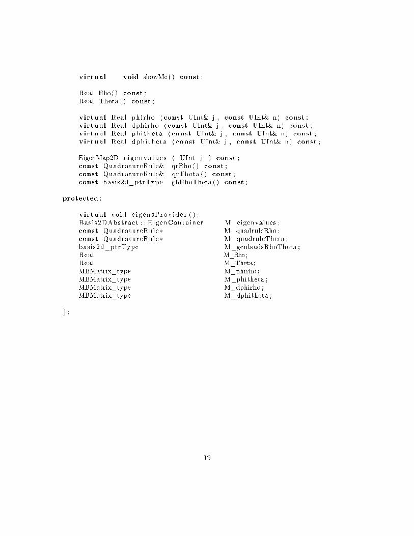
virtual void showMe ( ) const ;

Real Rho ( ) const ;Real Theta ( ) const ;

virtual Real phirho ( const UInt& j , const UInt& n) const ;virtual Real dphirho ( const UInt& j , const UInt& n) const ;virtual Real ph i theta ( const UInt& j , const UInt& n) const ;virtual Real dphitheta ( const UInt& j , const UInt& n) const ;

EigenMap2D e i g enva lu e s ( UInt j ) const ;const QuadratureRule& qrRho ( ) const ;const QuadratureRule& qrTheta ( ) const ;const basis2d_ptrType gbRhoTheta ( ) const ;

protected :

virtual void e i g en sProv ide r ( ) ;Basis2DAbstract : : EigenContainer M_eigenvalues ;const QuadratureRule∗ M_quadruleRho ;const QuadratureRule∗ M_quadruleTheta ;basis2d_ptrType M_genbasisRhoTheta ;Real M_Rho;Real M_Theta ;MBMatrix_type M_phirho ;MBMatrix_type M_phitheta ;MBMatrix_type M_dphirho ;MBMatrix_type M_dphitheta ;

;

19

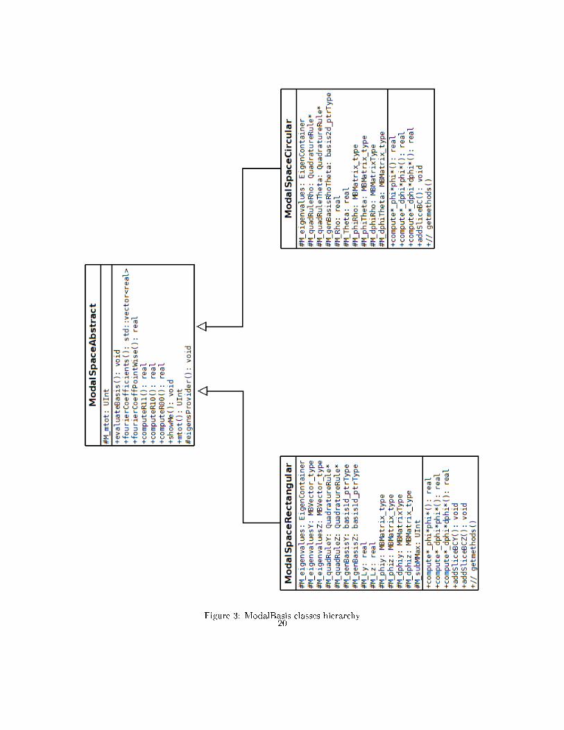
Figure 3: ModalBasis classes hierarchy20

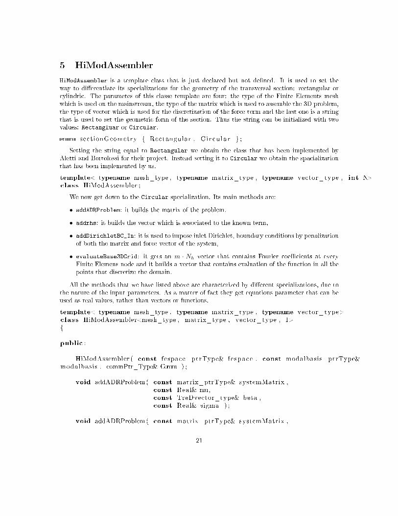
5 HiModAssembler

HiModAssembler is a template class that is just declared but not dened. It is used to set theway to dierentiate its specializations for the geometry of the transversal section: rectangular orcylindric. The parametes of this classe template are four: the type of the Finite Elements meshwhich is used on the mainstream, the type of the matrix which is used to assemble the 3D problem,the type of vector which is used for the discretization of the force term and the last one is a stringthat is used to set the geometric form of the section. Thus the string can be initialized with twovalues: Rectangluar or Circular.

enum sect ionGeometry Rectangular , C i r cu l a r ;

Setting the string equal to Rectangular we obtain the class that has been implemented byAletti and Bortolossi for their project. Instead setting it to Circular we obtain the spacializationthat has been implemented by us.

template< typename mesh_type , typename matrix_type , typename vector_type , int N>class HiModAssembler ;

We now get down to the Circular specialization. Its main methods are:

• addADRProblem: it builds the matrix of the problem,

• addrhs: it builds the vector which is associated to the known term,

• addDirichletBC_In: it is used to impose inlet Dirichlet, boundary conditions by penalizationof both the matrix and force vector of the system,

• evaluateBase3DGrid: it gets an m · Nh vector that contains Fourier coecients at everyFinite Elemens node and it builds a vector that contains evaluation of the function in all thepoints that discretize the domain.

All the methods that we have listed above are characterized by dierent specializations, due tothe nature of the input parameters. As a matter of fact they get equations parameter that can beused as real values, rather than vectors or functions.

template< typename mesh_type , typename matrix_type , typename vector_type>class HiModAssembler<mesh_type , matrix_type , vector_type , 1>

public :

HiModAssembler ( const fespace_ptrType& fespace , const modalbasis_ptrType&modalbasis , commPtr_Type& Comm ) ;

void addADRProblem( const matrix_ptrType& systemMatrix ,const Real& mu,const TreDvector_type& beta ,const Real& sigma ) ;

void addADRProblem( const matrix_ptrType& systemMatrix ,

21

const function_Type& mu,const function_Type& beta ,const function_Type& sigma ) ;

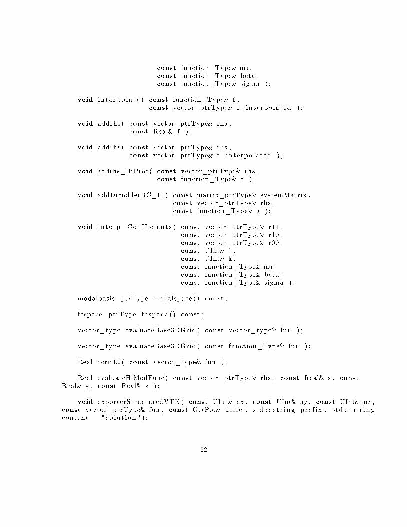
void i n t e r p o l a t e ( const function_Type& f ,const vector_ptrType& f_ in t e rpo l a t ed ) ;

void addrhs ( const vector_ptrType& rhs ,const Real& f ) ;

void addrhs ( const vector_ptrType& rhs ,const vector_ptrType& f_ in t e rpo l a t ed ) ;

void addrhs_HiPrec ( const vector_ptrType& rhs ,const function_Type& f ) ;

void addDirichletBC_In ( const matrix_ptrType& systemMatrix ,const vector_ptrType& rhs ,const function_Type& g ) ;

void i n t e r p_Coe f f i c i e n t s ( const vector_ptrType& r11 ,const vector_ptrType& r10 ,const vector_ptrType& r00 ,const UInt& j ,const UInt& k ,const function_Type& mu,const function_Type& beta ,const function_Type& sigma ) ;

modalbasis_ptrType modalspace ( ) const ;

fespace_ptrType f e spac e ( ) const ;

vector_type evaluateBase3DGrid ( const vector_type& fun ) ;

vector_type evaluateBase3DGrid ( const function_Type& fun ) ;

Real normL2( const vector_type& fun ) ;

Real evaluateHiModFunc ( const vector_ptrType& rhs , const Real& x , const

Real& y , const Real& z ) ;

void exporterStructuredVTK ( const UInt& nx , const UInt& ny , const UInt& nz ,const vector_ptrType& fun , const GetPot& d f i l e , s td : : s t r i n g p r e f i x , s td : : s t r i n gcontent = " s o l u t i o n " ) ;

22

void exporterFunctionVTK ( const UInt& nx , const UInt& ny , const UInt& nz ,const function_Type& f , const GetPot& d f i l e , s td : : s t r i n g p r e f i x , s td : : s t r i n gcontent = " func t i on " ) ;

private :

modalbasis_ptrType M_modalbasis ;et fespace_ptrType M_etfespace ;fespace_ptrType M_fespace ;

;

23

6 Numerical results

In this section we show you some numerical results we achieved and to visualize them we have usedParaView software. At rst we put the attention to a particular case for which solution is known apriori, so that we can compare the trend of numerical solution with the analytical one, varying thenumerical setting of the mesh and of the model reduction too. Then we considered more complexproblems for which analytical solution can't be expressed in closed form to get nearer to physicalphenomenons.

Problems of the rst type are enclosed in himod/tutorials and the are detached in dierentsubdirectories whose names have the structure kindofproblem_rect or kindofproblem_circ todistinguish the problems that are set on a cylinder with a rectangular section rather a circular one.Cases that have been studied by us are enclosed in the second type of subdirectories.

Problems of the second kind are enclosed in himod/testsuite and also in this case subdirecto-ries are dierentiated by the end of their name kindofproblem_rect or kindofproblem_circ todistinguish the problems that are set on a cylinder with a rectangular section rather a circular one.Cases that have been studied by us are enclosed in the second type of subdirectories.

Parameter setting is handled by user with parserGetPot so that no direct operations are neededon the code itself.

Theoretic support

As concerns the convergence error rate it is known an a priori error estimation that can be foundin [PZ13]

Theorem 1 Let us consider a domain Ω = Ω1 ⊗ Ω2.Provided a function u(x) ∈ V , x = (x1, x2) ∈ Ω ⊂ Rn,x1 ∈ Rn−1, x2 ∈ R so that V ⊂ H1(Ω)

and considering a set of basis functions ϕi(x2)∞i=1 ∈ H1(Ω2) so that:

uN (x) =

N∑i=0

ui(x1)ϕi(x2) ∀u ∈ V

it can be stated what follows:

‖u− uN‖L2(Ω) ≤ C(N + 1)−m‖Dmx2u‖L2(Ω),

‖u− uN‖H1(Ω) ≤ C(N + 1)1−m‖Dmx2u‖L2(Ω).

where m is a generic integer number, C ∈ R is a constant and N ∈ N is the index where the seriesexpansion is truncated.

Applying a Finite Element discretization on Ω1 this brings to a further theorem that can beapplied to our algorithm.

For this we introduce V 1h which is a nite-dimensional discretization ofH1(Ω1) by Finite Element

with h as a discretization step and r as the degree of the Lagrange polynomial functions. For sakeof simplicity we dene V 2

N as the subspace of H1(Ω2) which is detected by ϕiNi=1.

24

Theorem 2 Provided a function uhN (x) ∈ V 1h ⊗ V 2

N ,

uhN (x) =

N∑i=0

ui(x1)ϕi(x2)

it can be stated what follows:

‖u− uN‖L2(Ω) ≤ C[(N + 1)−m + h2r

][‖Dr

x1u‖L2(Ω) + ‖Dm

x2u‖L2(Ω)

].

Adopting this result to our case it means that the error in L2-normof the numerical solutioncomputed by Hi-Mod respect to the exact one is expected to scale as ( 1

m )2, while the error inH1-norm is expected to scale as ( 1

m ) because elliptic regularity results guarantee that a functionu ∈ H1(Ω), if Ω is convex, belongs to H2(Ω) too.

The Finite Element step has been set to be small enough so that we can neglect its contributionto the global error over the domain. Therefore the model error is the dominant one while mesherror is much smaller and doesn't aect the order of the global error.

For all the tests we did we set the mesh along the mainstream with 100 Finite Elements and onthe transversal section we used 50 modal functions.

Case test1

We have focused on a particular problems whose formulation is as follows:−µ∆u+ b · ∇u+ σu = f(x, ρ, θ) in Ω

u = 1− ρ2 on Γin

u′ = 0 onΓout

u = 0 ∂Ω \ (Γin ∪ Γout)

Ω = (x, ρ, θ) : 0 < x < 5, 0 < ρ < 1, 0 < θ < 2π,Γin = x = 0, 0 < ρ < 5, 0 < θ < 2π.

(19)

We set µ = 1, βx = 3, βρ = 1, βθ = 1. In order to have a solution that matches all the boundaryconditions we set the exact solution in this way:

ues(x, ρ, θ) = (1− ρ2)(5− x)2.

As a consequence the force term that we use to gure out numerical solution is:

f(x, ρ, θ) = µ(2ρ2 − 2 + 4(5− x)2)− 2bρρ(5− x)2 − bx(1− ρ2)(10− 2x)

Therefore to apply Hierarchical Model Reduction we used modal basis functions that are null onthe whole side of the cylinder. The trend of the solution is characterized by a parabolic prole atthe inlet section and the maximum value is reached along the axis of the cylinder. Moving towardsthe outlet section the parabolic prole on the transversal section is expected to decrease its peakprogressively due to the presence of the diusive term.

25

In the gures of the following page it is represented solution to (20) setting dierent number ofmodes along the transversal section. It can be noticed the fact that advection along the directionwhich is determined by the radius and the other one which is detected by the angle are deadenedby diusion. Instead something dierent from traditional Poisson problem is noticed for advectionalong the mainstream.

An improvement of the solution for an increase of the number of modes that are used along thetransversal section of the domain is noticeable both from solution's plot and from convergence ratetoo.

In our experiments we just computed L2-norm for the error and results are shown in the followingpages. You can notice that the empirical curve of the error is characterized by a linear order. It mayhave a sense because we are using bi-dimensional modal basis functions, while the theoretic resultsare presented using unidimensional Fourier series expansion. Anyway there are not well-knownresults about this probability yet. We make appeal to future works on this subject to explore thistopic.

In conclusion we present here a comparison between the errors that are related to 3D FiniteElements and Hierarchical Model Reduction setting the number of degrees of freedom the are usedon the transversal sections. It can be noticed that the curve which is associated with Hi-Modstays below the one that is related to Finite Elements and its slope is bigger too. This means thatHierarchical Model Reduction is a proper method to tackle the typical trade-o between expense ofcomputational cost (expressed by the number of degrees of freedom) and accuracy for the solutionthat is provided.

26

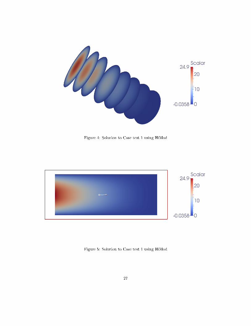
Figure 4: Solution to Case test 1 using HiMod

Figure 5: Solution to Case test 1 using HiMod

27

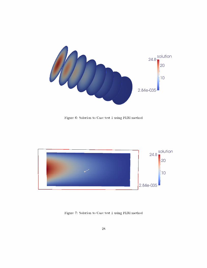
Figure 6: Solution to Case test 1 using FEM method

Figure 7: Solution to Case test 1 using FEM method

28

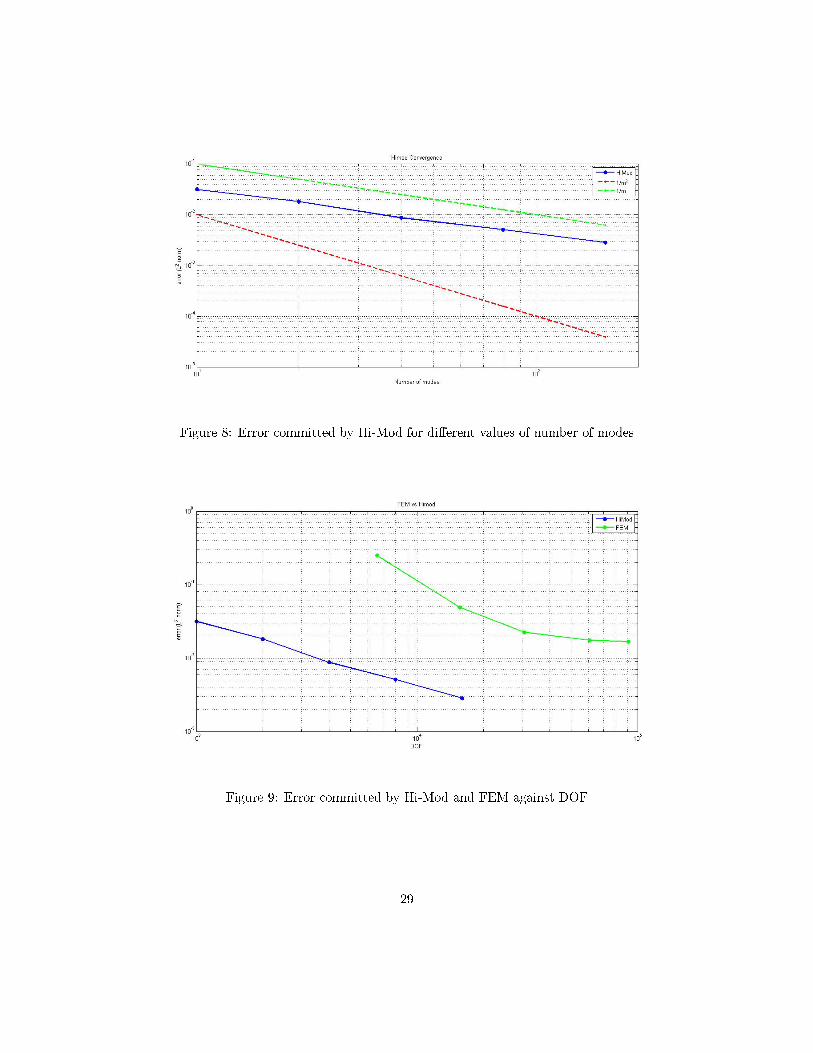
Figure 8: Error committed by Hi-Mod for dierent values of number of modes

Figure 9: Error committed by Hi-Mod and FEM against DOF

29

Case test 2

In this case test we aimed to analyze a problem which is nearer to real phenomenons. In detailwe wanted to model the advection of a medication by a blood in a vein due to the presence of astent on the wall. We modeled this object and the medication that it progressively releases using elocalized force term next to the wall of the domain.

Of course this complex and unsteady phenomenon is not exactly what we are going to reproduce,it is just an hint to what motivated us in setting the parameter of the equation in a certain wayrather than another.

Thus the formulation of the problem we have taken into account is the next one:−µ∆u+ b · ∇u+ σu = f in Ω

u = 1− ρ2 on Γin

u = 0 ∂Ω \ Γin

Ω = (x, ρ, θ) : 0 < x < 5, 0 < ρ < 1, 0 < θ < 2π,Γin = x = 0, 0 < ρ < 5, 0 < θ < 2π.

(20)

We set µ = 1, βx = 5, βρ = 0, βθ = 0. The force term is set to model the presence of an highconcentration of medication near the wall, this:

f(x, ρ, θ) =1[0.7,Lx3 ](x) ·1[0.7,1](ρ)

The solution which is provided by Hi-Mod is represented in the next page, near the full solutionto the same problem that was calculated using 3D Finite Element method. and it can be noticedthat the solutions coming from both the methods are very similar. To enforce this sentence weinserted a scheme where we plot the L2-norm distance between the full solution and the reducedone. It still happens that, increasing the number of modal basis functions to be used, the error israpidly cut down.

30

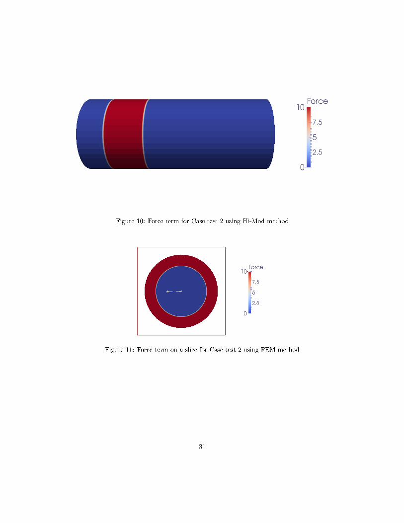
Figure 10: Force term for Case test 2 using Hi-Mod method

Figure 11: Force term on a slice for Case test 2 using FEM method

31

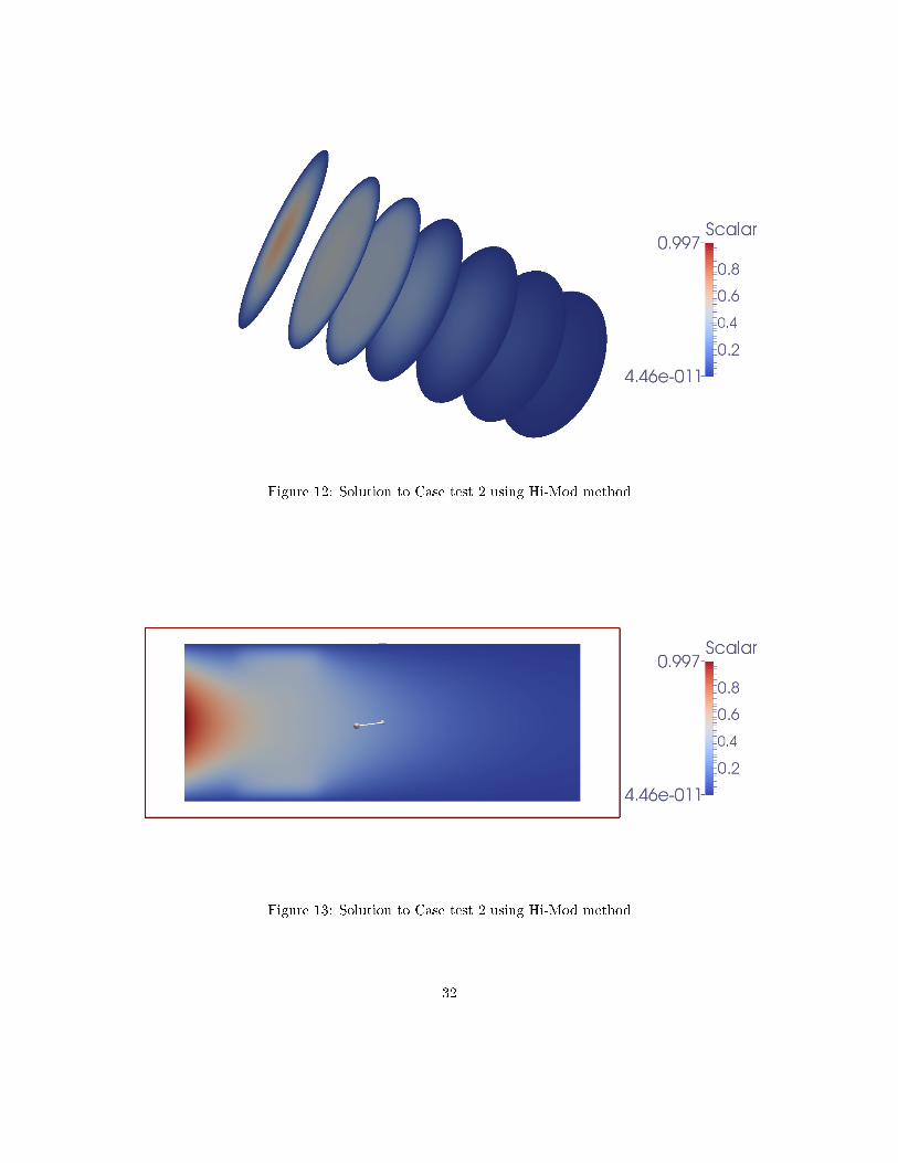
Figure 12: Solution to Case test 2 using Hi-Mod method

Figure 13: Solution to Case test 2 using Hi-Mod method

32

References

[AB13a] M. C. M. Aletti and A Bortolossi. Implementazioni in LifeV del metodo di RiduzioneGerarchica di Modello. Technical report, 2013.

[AB13b] M. C. M. Aletti and A. Bortolossi. Riduzione Gerarchica di Modello e Multiscala Geo-metrico. Technical report, 2013.

[EPV08] A. Ern, S. Perotto, and A. Veneziani. Hierarchical model reduction for advection-diusion-reaction problems. Springer Berlin Heidelberg, 2008.

[PEV] S. Perotto, A. Ern, and A. Veneziani. Coupled model and grid adaptivity in hierarchicalreduction of elliptic problems.

[PEV10] S. Perotto, A. Ern, and A. Veneziani. Hierarchical Local Model Rediction for EllipticProblems: a Domain Decomposition Approach. Multiscale Modeling and Simulation,8(4):11021127, 2010.

[PZ13] S. Perotto and A. Zilio. Hierarchical Model Reduction: Three Dierent Approaches. 2013.

[Qua08] A. Quarteroni. Modellistica numerica per problemi dierenziali. Springer, Milan, 4 edition,2008.

[Sal10] S. Salsa. Equazioni a derivate parziali. Metodi, modelli e applicazioni. Springer, Milan, 2edition, 2010.

[Str86] G. Strang. Introduction to Applied Mathematics. Wellesley Cambridge Pr, 1986.

[ZJ96] S. Zhang and J. Jin. Computation of Special Functions. John Wiley and Sons, Inc., 1996.

33