Use of In Situ Sensors for Wire Fault Prognostics

Dr. Chet Lo, Dr. Cynthia Furse*,**

*Department of Electrical and Computer Engineering University of Utah

Salt Lake City, Utah

**LiveWire Test Labs, Inc. Salt Lake City, Utah

I. Introduction

The past decade has been a time of very fruitful research in EWIS, with advances in wire analysis, repair, and testing techniques. As these technologies and methods mature and are implemented, they promise tremendous improvements in the ability to monitor and maintain wiring systems. As our diagnostic sensors improve, it makes sense to evaluate the possibility of using them for prognostics as well. The ability to locate intermittent open and short circuits has already been demonstrated in the laboratory and is being developed into a full scale on board test system. Locating less pronounced problems (high impedance shorts, for instance, or small impedance changes in the connection to the ground plane) is much more difficult. The ‘Holy Grail’ of wire testing is the ability to locate very small faults soon enough that they can safely be left until the aircraft is scheduled for routine maintenance, rather than having to find and fix a fault on the flight line. Finding the small anomalies of frayed wire before they become hard open or short circuits is of significant interest; however it is an extremely difficult problem. Chafing insulation from the conductor results in a very small change in the wire impedance. Even major chafes to the conductor itself result in large changes locally that have been found to be undetectable in the randomly varying environment of aircraft and other vibrating systems. [5] For systems that rely on reflectometry, this results in a very small reflection that may be lost in the noise of the measurements. Some authors have reported success locating frays in a controlled laboratory environment. In [1], TDR is used to detect bends, heating, and compression in coaxial and unshielded wiring, in a controlled setting where the wire is not allowed to move around, is isolated from other wires, and from the physical structure of the plane. In [2][3] we observed that frays are more observable at high frequencies than low frequencies. In [4] a method for using a sliding correlator to locate the signature of the fray from within the other noise on the wire was shown to be effective even for very small faults in a highly controlled setting. Unfortunately, in settings where vibration and other noise sources corrupt the data, this method is not enough to pull the very small reflection signals out of the noise. With these early analyses, there could be some hope for location of frays, however it should be noted that these tests were done in a very controlled laboratory environments. In [5] TDR, FDR, and SSTDR were evaluated on small frays, large frays, water drops on the wire, and normal movement of the wires. These reflections were compared to those observed from ‘normal’ changes in the wires such as vibration and drops of water on the wire. The reflections due to normal environmental changes were found to be larger than those induced by frayed insulation and other small faults, thus making it virtually impossible to locate frays from the reflectometry signature alone. An exception to this is the intermittent fault, which is actually a short or open circuit, albeit for a very short time. These may be located, if a reflectometry system is in operation on the wire while the fault is present. This paper considers a different possibility. Rather than attempting to locate the very small faults caused by frayed insulation or conductor from the reflectometry signature in a vibrating environment, this paper assesses the ability to locate other physical precursors to fray-type faults. Since these faults are often caused by improperly installed wire ties or clamps (or ties/clamps that come loose), assessment of the environmental changes associated with vibration of wiring may have very interesting and potentially useful signatures. A single vibrating wire will move closer and further from the ground plane (or from a secondary wire used as a ground return path), thus changing its impedance in predictable and time periodic ways. In particular, aircraft wiring is clamped to metallic struts at 1-2 foot increments. Between the clamps the wire has its maximum vibration, and at the clamps the vibration is minimized. Once the physical connections, clamps, ties, etc. of the wiring harness are established, its vibration signature should

remain the same over time. If a tie comes loose, thus increasing the probability of fraying the wire, the change in signature may be able to predict its location. The vibration signature also provides a threshold for expected detection of the reflectometry response. This threshold varies along the length of the wire, depending on the vibration at each location, thus allowing more sensitivity in some areas than in others. This paper assesses the ability to use reflectometry to identify both the vibration response along the length of the wire and the reflectometry response of individual faults that are superimposed on this vibration response. Theoretical modeling and computer simulations are used in this study, which are supported by preliminary measurements. In the following sections, we study the simulation of sensors in response to common wire conditions and compare the simulations to physical measurements. Next, after the simulation is verified, we simulate cases several vibration characteristics. Finally, we discuss the implications of these simulations, the ability to detect different faults with different sensor types, and risk profiles along the wire harness through different physical structures.

II. Simulation Methods Detailed simulation methods are needed in order to predict the reflectometry responses to vibration and faults. Three reflectometry methods were evaluated. Time Domain Reflectometry (TDR) uses a step function or pulse as the test function on the wire. This pulse propagates down the wire until it gets to an impedance discontinuity, where it reflects back to the source and is received and evaluated. The time delay between the incident and reflected pulses depends on the distance to the impedance discontinuity and the velocity of propagation on the wire. The magnitude and polarity of the returning pulse depends on the magnitude of the impedance discontinuity. Frays have very small effective impedance discontinuities, while open and short circuits (and branches in the wiring) have much larger discontinuities. Frequency domain reflectometry (FDR) uses a set of sine waves of several individual frequencies, each of which reflects back with a phase shift proportional to the distance to the fault and with a magnitude proportional to the magnitude of the fault. Spectral (STDR) and spread spectrum time domain reflectometry (SSTDR) use a pseudo noise (PN) code or a sine wave modulated PN code as the incident signal. Correlation with the original code gives the distance to and nature of the fault. Each of these reflectometry methods provides responses that can be used to derive the location of the wire fault based on the time delay and magnitude of the response. [6] The simulations used in this paper are somewhat different than those used previously. The very small reflections that occur along the full length of the wire require special attention. Two simulation methods are explored in this research. First is the finite-difference time-domain (FDTD) approach [7], and second, the generalized bouncing diagram (GBD) approach. [8] Both represent the time domain response on the wire starting with transmission line models of the system being considered. The impedance at every point is calculated using either analytical approaches [9] for wires that are simply separated from each other or from the ground plane or the finite-difference frequency-domain (FDFD) method [7] which is used to model wiring faults in [5]. FDTD converts the time domain differential form of Maxwell’s equations to a discrete difference form and solves for the voltage on the line as a function of time. This is the reflectometry response that is desired. The GBD method also calculates the reflectometry response, but by subdivides the wire into small sections. According to the local physical dimensions of the wire, the impedances is determined for each of the small sections. The attenuation of the signal as it passes through each section is also calculated. This depends on frequency, length of that section, wire type and dimension, etc. Thus, each section of wire acts like a frequency-dependent filter. [9] The transmission and reflection coefficients the determine how much power is transmitted to other sections of the wire and how much is reflected back are determined between neighboring sections according to their impedances. [9] Both the FDTD and GBD methods use a time domain incident signal fs(t) and determine the time domain response of the wire system h(t). For these simulations a sinc function (sin(t)/t) was used as the incident signal fs(t) . This was chosen, because it includes equal-magnitude frequency components for all frequencies and can therefore easily be converted to other signatures of interest (such as S/SSTDR, FDR). The impulse response of the wire is h(t). The output of the FDTD/GBD simulation is fs(t) convolved with the response of the wire h(t), or the signature that would be obtained if we could run the time domain

simulations with an impulse response (which we can’t). In other words, the time domain response, or the FDTD or GBD simulation, obtained from the incident sinc function fs(t) on the wire system h(t) is fs(t) * h(t), where * means time domain convolution. However, the incident function we are really interested in is the one used by the specific sensor we are simulating (in our case this is an S/SSTDR). Let the incident signature of the specific sensor be f(t). The response of the system (the results that would be measured using S/SSTDR) g(t) can then be found by convolving f(t) with h(t):

( ) ( )* ( )g t f t h t= . As fs(t) has a flat frequency response in its pass band, if we have fs(t)’s pass band wider the that of f(t)’s, we can have:

( ) ( )* ( ) ( )*[ ( )* ( )]sg t f t h t f t f t h t= =

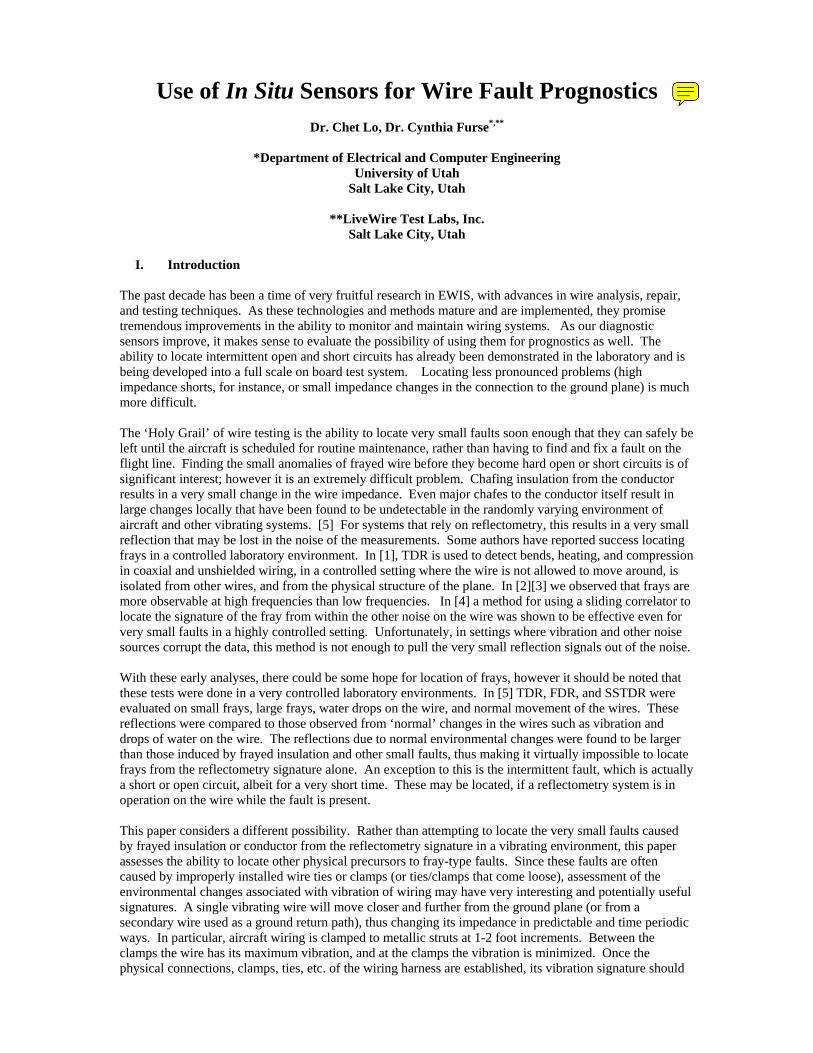
The second part of this equation shows that the FDTD or GBD simulation can be used to determine g(t). Thus, we run our FDTD or GBD simulation with a sinc function and extract its response. We can then obtain the expected response of the S/SSTDR signature by convolving the desired incident signature with the simulated signature. In Figure 1, we show the sinc function simulation results from both FDTD and GBD for a section of wire 2 feet long with an open circuit at the end. The FDTD response shows the reflected sinc function at 2 feet, as expected. The GBD signature also gives a reflected sinc function, although it is narrower. After convolving both of these simulations with the desired SSTDR pulse, the results are very similar, as shown in Figure 1. The GBD method was used for the remaining simulations in this paper because of its ease of use.

0 2 4 6 8 10-0.05

0

0.05

0.1

0.15

Mag

nitu

de

Distance (ft)

Simulation result of FDTD

0 1 2 3 4 5-0.5

0

0.5

1

Mag

nitu

de

Distance (ft)

Simulation result of GBD

-5 0 5 10 15-1

-0.5

0

0.5

1

Mag

nitu

de

Distance (ft)

FDTD result after conv with SSTDR pulse

-5 0 5 10 15-1

-0.5

0

0.5

1

Mag

nitu

de

Distance (ft)

GBD result after conv with SSTDR pulse

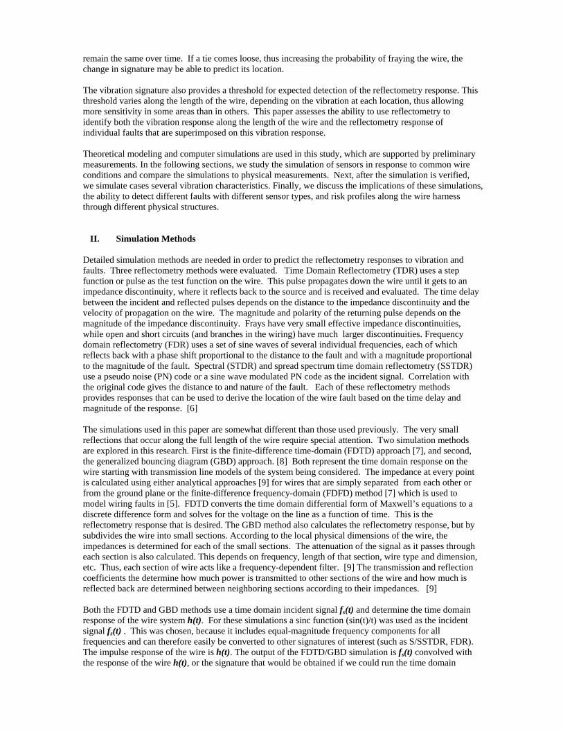
Figure 1 Comparison of FDTD and GBD simulation results for an SSTDR pulse A significant consideration when converting the time domain responses obtained from reflectometry (and from the FDTD and GBD simulations) is the velocity of propagation. Reflectometry gives a measurement of reflection as a function of TIME, but we are interested in faults along the DISTANCE along the wire. The distance is found by multiplying the velocity of propagation by the time. The velocity of propagation has been found to vary slightly within bundles of wires [6]. For our evaluation, it is important to know how the velocity of propagation changes as a function of distance between the wire under test and its ground plane. In Figure 2, we show the propagation speed normalized by the speed of light (c) versus wire separation. The wires in this case are 1mm radius copper wires with no insulation (and they are not touching). We can see that the propagation speed is practically constant, 0.6887c in this case. Insulation on the wires has very small effect on this velocity of propagation. Thus, we did not change the velocity of propagation in our simulation regions, regardless of the separation of the wires.

0 1 2 3 4 5 6 7 8 9 100.6887

0.6887

0.6887

0.6887

0.6887

0.6887

0.6887

Wire Separation (ft)

Prop

agat

ion

Spe

ed (c

)

Figure 2 Propagation speed versus wire separation for 0.04” radius copper wires with polyethylene as insulation. III. Validity of the Simulation

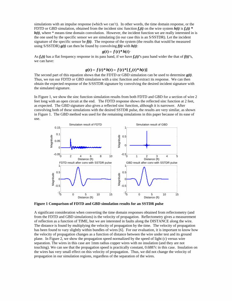
We will establish the legitimacy of our simulation in this section by comparing simulation of STDR signature with measured STDR signature. This verification applies to other kind of sensors as well as we discussed in the section about test signals. We will at the same time observe the changes in reflectometry signature cause by changes in wire separation alone. We expect to see changes in reflectometry signature as the local impedance of the conducting wire is linearly proportional to the log of wire separation as shown in Figure 3.

10-3

10-2

10-1

100

101200

400

600

800

1000

Wire Separation (ft)

Impe

danc

e (Ω

)

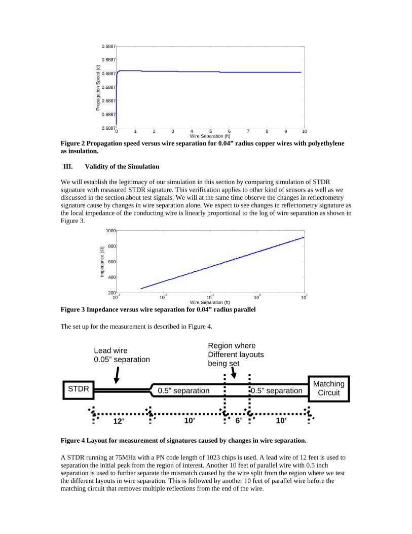
Figure 3 Impedance versus wire separation for 0.04” radius parallel The set up for the measurement is described in Figure 4.

Figure 4 Layout for measurement of signatures caused by changes in wire separation. A STDR running at 75MHz with a PN code length of 1023 chips is used. A lead wire of 12 feet is used to separation the initial peak from the region of interest. Another 10 feet of parallel wire with 0.5 inch separation is used to further separate the mismatch caused by the wire split from the region where we test the different layouts in wire separation. This is followed by another 10 feet of parallel wire before the matching circuit that removes multiple reflections from the end of the wire.

STDR MatchingCircuit

12’ 10’ 10’ 6’

Lead wire 0.05” separation

Region where Different layouts being set

0.5” separation 0.5” separation

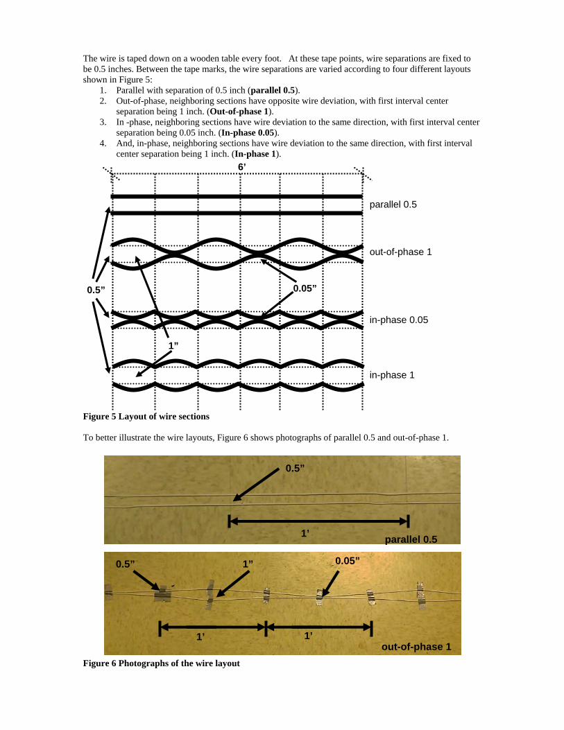
The wire is taped down on a wooden table every foot. At these tape points, wire separations are fixed to be 0.5 inches. Between the tape marks, the wire separations are varied according to four different layouts shown in Figure 5:

1. Parallel with separation of 0.5 inch (parallel 0.5). 2. Out-of-phase, neighboring sections have opposite wire deviation, with first interval center

separation being 1 inch. (Out-of-phase 1). 3. In -phase, neighboring sections have wire deviation to the same direction, with first interval center

separation being 0.05 inch. (In-phase 0.05). 4. And, in-phase, neighboring sections have wire deviation to the same direction, with first interval

center separation being 1 inch. (In-phase 1).

Figure 5 Layout of wire sections To better illustrate the wire layouts, Figure 6 shows photographs of parallel 0.5 and out-of-phase 1.

Figure 6 Photographs of the wire layout

6’

0.5”

1”

0.05”

parallel 0.5

out-of-phase 1

in-phase 0.05

in-phase 1

1’

0.5”

1’ 1’

0.5” 1” 0.05”

out-of-phase 1

parallel 0.5

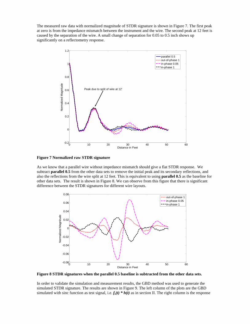
The measured raw data with normalized magnitude of STDR signature is shown in Figure 7. The first peak at zero is from the impedance mismatch between the instrument and the wire. The second peak at 12 feet is caused by the separation of the wire. A small change of separation for 0.05 to 0.5 inch shows up significantly on a reflectometry response.

0 10 20 30 40 50 60-0.2

0

0.2

0.4

0.6

0.8

1

1.2

Distance in Feet

Nor

mal

ized

Mag

nitu

de

parallel 0.5out-of-phase 1in-phase 0.05in-phase 1

Peak due to split of wire at 12'

Figure 7 Normalized raw STDR signature As we know that a parallel wire without impedance mismatch should give a flat STDR response. We subtract parallel 0.5 from the other data sets to remove the initial peak and its secondary reflections, and also the reflections from the wire split at 12 feet. This is equivalent to using parallel 0.5 as the baseline for other data sets. The result is shown in Figure 8. We can observe from this figure that there is significant difference between the STDR signatures for different wire layouts.

0 10 20 30 40 50 60-0.08

-0.06

-0.04

-0.02

0

0.02

0.04

0.06

0.08

Distance in Feet

Nor

mal

ized

Mag

nitu

de

out-of-phase 1in-phase 0.05in-phase 1

Figure 8 STDR signatures when the parallel 0.5 baseline is subtracted from the other data sets. In order to validate the simulation and measurement results, the GBD method was used to generate the simulated STDR signature. The results are shown in Figure 9. The left column of the plots are the GBD simulated with sinc function as test signal, i.e. fs(t) * h(t) as in section II. The right column is the response

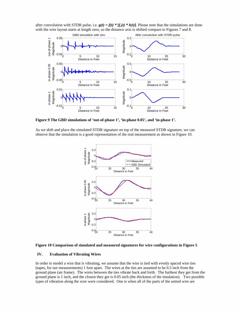
after convolution with STDR pulse, i.e. g(t) = f(t) * [fs(t) * h(t)]. Please note that the simulations are done with the wire layout starts at length zero, so the distance axis is shifted compare to Figures 7 and 8.

0 5 10 15-0.05

0

0.05

Distance in Feet

out-o

f-pha

se 1

M

agni

tude

GBD simulation with sinc

0 10 20 30-0.2

0

0.2

Distance in Feet

Mag

nitu

de

After convolution with STDR pulse

0 5 10 15-0.05

0

0.05

Distance in Feet

in-p

hase

0.0

5 M

agni

tude

0 10 20 30-0.5

0

0.5

Distance in Feet

Mag

nitu

de

0 5 10 15-0.01

0

0.01

Distance in Feet

in-p

hase

1

Mag

nitu

de

0 10 20 30-0.1

0

0.1

Distance in Feet

Mag

nitu

de

Figure 9 The GBD simulations of ‘out-of-phase 1’, ‘in-phase 0.05’, and ‘in-phase 1’. As we shift and place the simulated STDR signature on top of the measured STDR signature, we can observe that the simulation is a good representation of the real measurement as shown in Figure 10.

20 25 30 35 40-0.4

-0.2

0

0.2

Distance in Feet

out-o

f-pha

se 1

M

agni

tude

20 25 30 35 40-0.4

-0.2

0

0.2

Distance in Feet

in-p

hase

0.0

5 M

agni

tude

20 25 30 35 40-0.4

-0.2

0

0.2

Distance in Feet

in-p

hase

1

Mag

nitu

de

MeasuredGBD Simulated

Figure 10 Comparison of simulated and measured signatures for wire configurations in Figure 5 IV. Evaluation of Vibrating Wires

In order to model a wire that is vibrating, we assume that the wire is tied with evenly spaced wire ties (tapes, for our measurements) 1 foot apart. The wires at the ties are assumed to be 0.5 inch from the ground plane (air frame). The wires between the ties vibrate back and forth. The furthest they get from the ground plane is 1 inch, and the closest they get is 0.05 inch (the thickness of the insulation). Two possible types of vibration along the wire were considered. One is when all of the parts of the untied wire are

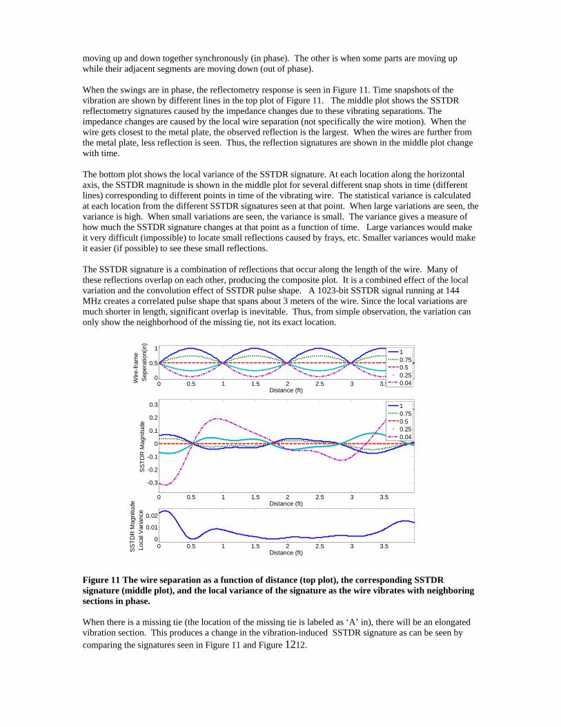
moving up and down together synchronously (in phase). The other is when some parts are moving up while their adjacent segments are moving down (out of phase). When the swings are in phase, the reflectometry response is seen in Figure 11. Time snapshots of the vibration are shown by different lines in the top plot of Figure 11. The middle plot shows the SSTDR reflectometry signatures caused by the impedance changes due to these vibrating separations. The impedance changes are caused by the local wire separation (not specifically the wire motion). When the wire gets closest to the metal plate, the observed reflection is the largest. When the wires are further from the metal plate, less reflection is seen. Thus, the reflection signatures are shown in the middle plot change with time. The bottom plot shows the local variance of the SSTDR signature. At each location along the horizontal axis, the SSTDR magnitude is shown in the middle plot for several different snap shots in time (different lines) corresponding to different points in time of the vibrating wire. The statistical variance is calculated at each location from the different SSTDR signatures seen at that point. When large variations are seen, the variance is high. When small variations are seen, the variance is small. The variance gives a measure of how much the SSTDR signature changes at that point as a function of time. Large variances would make it very difficult (impossible) to locate small reflections caused by frays, etc. Smaller variances would make it easier (if possible) to see these small reflections. The SSTDR signature is a combination of reflections that occur along the length of the wire. Many of these reflections overlap on each other, producing the composite plot. It is a combined effect of the local variation and the convolution effect of SSTDR pulse shape. A 1023-bit SSTDR signal running at 144 MHz creates a correlated pulse shape that spans about 3 meters of the wire. Since the local variations are much shorter in length, significant overlap is inevitable. Thus, from simple observation, the variation can only show the neighborhood of the missing tie, not its exact location.

0 0.5 1 1.5 2 2.5 3 3.50

0.5

1

Distance (ft)

Wire

-fram

e S

eper

atio

n(in

)

0 0.5 1 1.5 2 2.5 3 3.5

-0.3

-0.2

-0.1

0

0.1

0.2

0.3

Distance (ft)

SS

TDR

Mag

nitu

de

0 0.5 1 1.5 2 2.5 3 3.50

0.01

0.02

Distance (ft)SS

TDR

Mag

nitu

de

Loc

al V

aria

nce

10.750.50.250.04

10.750.50.250.04

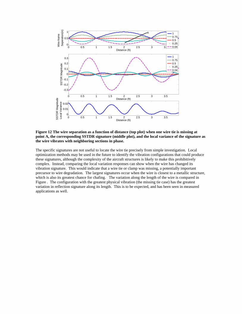
Figure 11 The wire separation as a function of distance (top plot), the corresponding SSTDR signature (middle plot), and the local variance of the signature as the wire vibrates with neighboring sections in phase. When there is a missing tie (the location of the missing tie is labeled as ‘A’ in), there will be an elongated vibration section. This produces a change in the vibration-induced SSTDR signature as can be seen by comparing the signatures seen in Figure 11 and Figure 1212.

0 0.5 1 1.5 2 2.5 3 3.50

0.5

1

Distance (ft)

Wire

-fram

e S

eper

atio

n(in

)

10.750.50.250.04

0 0.5 1 1.5 2 2.5 3 3.5

-0.3

-0.2

-0.1

0

0.1

0.2

0.3

Distance (ft)

SS

TDR

Mag

nitu

de

10.750.50.250.04

0 0.5 1 1.5 2 2.5 3 3.50

0.01

0.02

Distance (ft)SS

TDR

Mag

nitu

de

Loc

al V

aria

nce

A

Figure 12 The wire separation as a function of distance (top plot) when one wire tie is missing at point A, the corresponding SSTDR signature (middle plot), and the local variance of the signature as the wire vibrates with neighboring sections in phase. The specific signatures are not useful to locate the wire tie precisely from simple investigation. Local optimization methods may be used in the future to identify the vibration configurations that could produce these signatures, although the complexity of the aircraft structures is likely to make this prohibitively complex. Instead, comparing the local variation responses can show when the wire has changed its vibration signature. This would indicate that a wire tie or clamp was missing, a potentially important precursor to wire degradation. The largest signatures occur when the wire is closest to a metallic structure, which is also its greatest chance for chafing. The variation along the length of the wire is compared in Figure . The configuration with the greatest physical vibration (the missing tie case) has the greatest variation in reflection signature along its length. This is to be expected, and has been seen in measured applications as well.

0 0.5 1 1.5 2 2.5 3 3.5

0

0.005

0.01

0.015

0.02

0.025

Distance (ft)

SS

TDR

Mag

nitu

de

Loc

al V

aria

nce

No missing tieWith missing tie

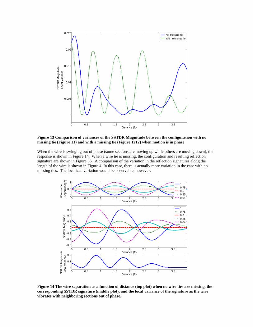
Figure 13 Comparison of variances of the SSTDR Magnitude between the configuration with no missing tie (Figure 11) and with a missing tie (Figure 1212) when motion is in phase When the wire is swinging out of phase (some sections are moving up while others are moving down), the response is shown in Figure 14. When a wire tie is missing, the configuration and resulting reflection signature are shown in Figure 35. A comparison of the variation in the reflection signatures along the length of the wire is shown in Figure 4. In this case, there is actually more variation in the case with no missing ties. The localized variation would be observable, however.

0 0.5 1 1.5 2 2.5 3 3.50

0.5

1

Distance (ft)

Wire

-fram

e S

eper

atio

n(in

)

10.750.50.250.04

0 0.5 1 1.5 2 2.5 3 3.5-0.6

-0.4

-0.2

0

0.2

0.4

0.6

Distance (ft)

SS

TDR

Mag

nitu

de

10.750.50.250.04

0 0.5 1 1.5 2 2.5 3 3.50

0.1

0.2

Distance (ft)SS

TDR

Mag

nitu

de

Loc

al V

aria

nce

Figure 14 The wire separation as a function of distance (top plot) when no wire ties are missing, the corresponding SSTDR signature (middle plot), and the local variance of the signature as the wire vibrates with neighboring sections out of phase.

0 0.5 1 1.5 2 2.5 3 3.50

0.5

1

Distance (ft)

Wire

-fram

e S

eper

atio

n(in

)

0 0.5 1 1.5 2 2.5 3 3.5-0.8

-0.6

-0.4

-0.2

0

0.2

0.4

0.6

Distance (ft)

SS

TDR

Mag

nitu

de

0 0.5 1 1.5 2 2.5 3 3.50

0.1

0.2

Distance (ft)SS

TDR

Mag

nitu

de

Loc

al V

aria

nce

10.750.50.250.04

10.750.50.250.04

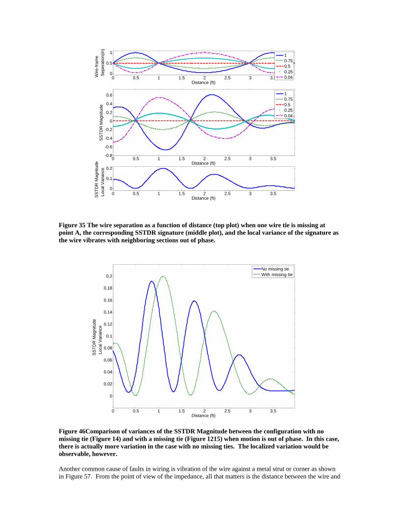
Figure 35 The wire separation as a function of distance (top plot) when one wire tie is missing at point A, the corresponding SSTDR signature (middle plot), and the local variance of the signature as the wire vibrates with neighboring sections out of phase.

0 0.5 1 1.5 2 2.5 3 3.5

0

0.02

0.04

0.06

0.08

0.1

0.12

0.14

0.16

0.18

0.2

Distance (ft)

SS

TDR

Mag

nitu

de

Loc

al V

aria

nce

No missing tieWith missing tie

Figure 46Comparison of variances of the SSTDR Magnitude between the configuration with no missing tie (Figure 14) and with a missing tie (Figure 1215) when motion is out of phase. In this case, there is actually more variation in the case with no missing ties. The localized variation would be observable, however. Another common cause of faults in wiring is vibration of the wire against a metal strut or corner as shown in Figure 57. From the point of view of the impedance, all that matters is the distance between the wire and

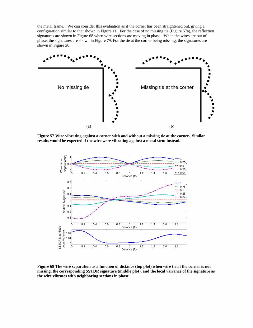
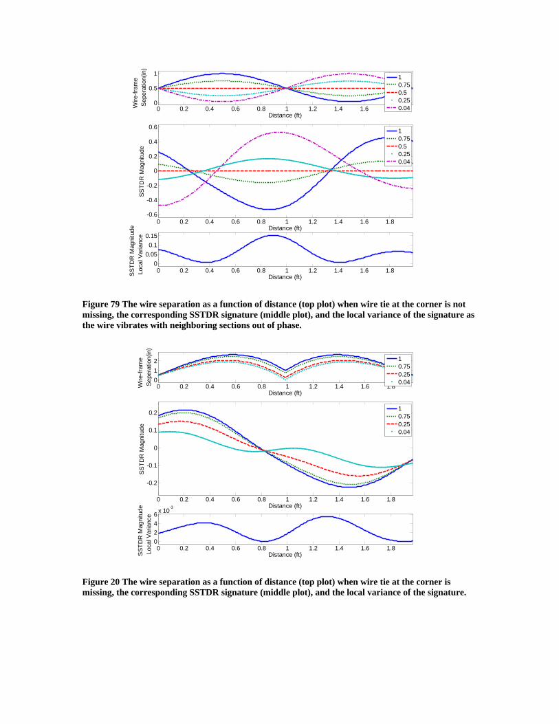
the metal frame. We can consider this evaluation as if the corner has been straightened out, giving a configuration similar to that shown in Figure 11. For the case of no missing tie (Figure 57a), the reflection signatures are shown in Figure 68 when wire sections are moving in phase. When the wires are out of phase, the signatures are shown in Figure 79. For the tie at the corner being missing, the signatures are shown in Figure 20.

(a) (b)

Figure 57 Wire vibrating against a corner with and without a missing tie at the corner. Similar results would be expected if the wire were vibrating against a metal strut instead.

0 0.2 0.4 0.6 0.8 1 1.2 1.4 1.6 1.80

0.5

1

Distance (ft)

Wire

-fram

e S

eper

atio

n(in

)

10.750.50.250.04

0 0.2 0.4 0.6 0.8 1 1.2 1.4 1.6 1.8

-0.3

-0.2

-0.1

0

0.1

0.2

0.3

Distance (ft)

SS

TDR

Mag

nitu

de

10.750.50.250.04

0 0.2 0.4 0.6 0.8 1 1.2 1.4 1.6 1.80

0.01

0.02

Distance (ft)SS

TDR

Mag

nitu

de

Loc

al V

aria

nce

Figure 68 The wire separation as a function of distance (top plot) when wire tie at the corner is not missing, the corresponding SSTDR signature (middle plot), and the local variance of the signature as the wire vibrates with neighboring sections in phase.

No missing tie Missing tie at the corner

0 0.2 0.4 0.6 0.8 1 1.2 1.4 1.6 1.80

0.5

1

Distance (ft)

Wire

-fram

e S

eper

atio

n(in

)

0 0.2 0.4 0.6 0.8 1 1.2 1.4 1.6 1.8-0.6

-0.4

-0.2

0

0.2

0.4

0.6

Distance (ft)

SS

TDR

Mag

nitu

de

0 0.2 0.4 0.6 0.8 1 1.2 1.4 1.6 1.80

0.050.1

0.15

Distance (ft)SS

TDR

Mag

nitu

de

Loc

al V

aria

nce

10.750.50.250.04

10.750.50.250.04

Figure 79 The wire separation as a function of distance (top plot) when wire tie at the corner is not missing, the corresponding SSTDR signature (middle plot), and the local variance of the signature as the wire vibrates with neighboring sections out of phase.

0 0.2 0.4 0.6 0.8 1 1.2 1.4 1.6 1.8012

Distance (ft)

Wire

-fram

e S

eper

atio

n(in

)

0 0.2 0.4 0.6 0.8 1 1.2 1.4 1.6 1.8

-0.2

-0.1

0

0.1

0.2

Distance (ft)

SS

TDR

Mag

nitu

de

0 0.2 0.4 0.6 0.8 1 1.2 1.4 1.6 1.80246 x 10

-3

Distance (ft)SST

DR

Mag

nitu

de

Loc

al V

aria

nce

10.750.250.04

10.750.250.04

Figure 20 The wire separation as a function of distance (top plot) when wire tie at the corner is missing, the corresponding SSTDR signature (middle plot), and the local variance of the signature.

0 0.2 0.4 0.6 0.8 1 1.2 1.4 1.6 1.8

0

0.02

0.04

0.06

0.08

0.1

0.12

0.14

0.16

SS

TDR

Mag

nitu

de L

ocal

Var

ianc

e

Distance (ft)

No missing tie (in phase)No missing tie (out-of-phase)With missing tie

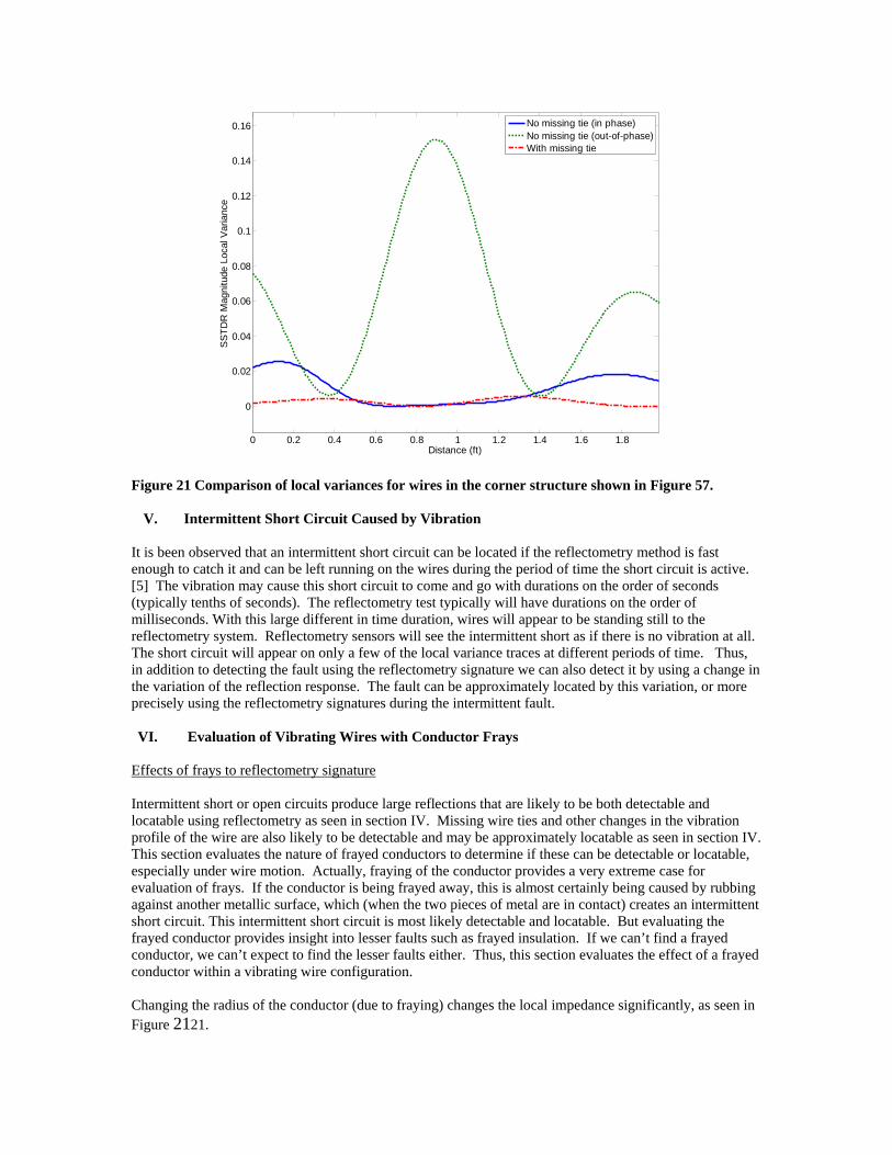
Figure 21 Comparison of local variances for wires in the corner structure shown in Figure 57.

V. Intermittent Short Circuit Caused by Vibration

It is been observed that an intermittent short circuit can be located if the reflectometry method is fast enough to catch it and can be left running on the wires during the period of time the short circuit is active. [5] The vibration may cause this short circuit to come and go with durations on the order of seconds (typically tenths of seconds). The reflectometry test typically will have durations on the order of milliseconds. With this large different in time duration, wires will appear to be standing still to the reflectometry system. Reflectometry sensors will see the intermittent short as if there is no vibration at all. The short circuit will appear on only a few of the local variance traces at different periods of time. Thus, in addition to detecting the fault using the reflectometry signature we can also detect it by using a change in the variation of the reflection response. The fault can be approximately located by this variation, or more precisely using the reflectometry signatures during the intermittent fault. VI. Evaluation of Vibrating Wires with Conductor Frays

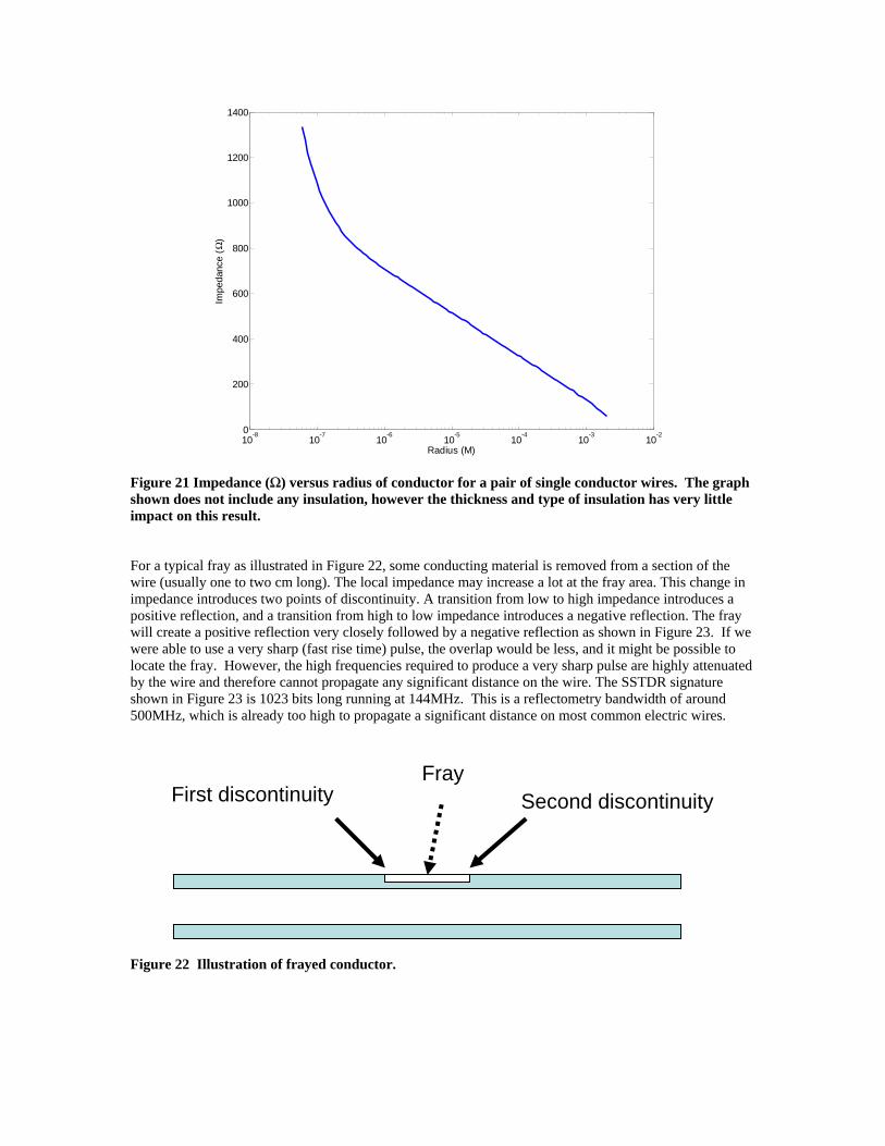
Effects of frays to reflectometry signature Intermittent short or open circuits produce large reflections that are likely to be both detectable and locatable using reflectometry as seen in section IV. Missing wire ties and other changes in the vibration profile of the wire are also likely to be detectable and may be approximately locatable as seen in section IV. This section evaluates the nature of frayed conductors to determine if these can be detectable or locatable, especially under wire motion. Actually, fraying of the conductor provides a very extreme case for evaluation of frays. If the conductor is being frayed away, this is almost certainly being caused by rubbing against another metallic surface, which (when the two pieces of metal are in contact) creates an intermittent short circuit. This intermittent short circuit is most likely detectable and locatable. But evaluating the frayed conductor provides insight into lesser faults such as frayed insulation. If we can’t find a frayed conductor, we can’t expect to find the lesser faults either. Thus, this section evaluates the effect of a frayed conductor within a vibrating wire configuration. Changing the radius of the conductor (due to fraying) changes the local impedance significantly, as seen in Figure 2121.

10-8

10-7

10-6

10-5

10-4

10-3

10-20

200

400

600

800

1000

1200

1400

Radius (M)

Impe

danc

e (Ω

)

Figure 21 Impedance (Ω) versus radius of conductor for a pair of single conductor wires. The graph shown does not include any insulation, however the thickness and type of insulation has very little impact on this result. For a typical fray as illustrated in Figure 22, some conducting material is removed from a section of the wire (usually one to two cm long). The local impedance may increase a lot at the fray area. This change in impedance introduces two points of discontinuity. A transition from low to high impedance introduces a positive reflection, and a transition from high to low impedance introduces a negative reflection. The fray will create a positive reflection very closely followed by a negative reflection as shown in Figure 23. If we were able to use a very sharp (fast rise time) pulse, the overlap would be less, and it might be possible to locate the fray. However, the high frequencies required to produce a very sharp pulse are highly attenuated by the wire and therefore cannot propagate any significant distance on the wire. The SSTDR signature shown in Figure 23 is 1023 bits long running at 144MHz. This is a reflectometry bandwidth of around 500MHz, which is already too high to propagate a significant distance on most common electric wires.

Figure 22 Illustration of frayed conductor.

First discontinuity Second discontinuityFray

-3 -2 -1 0 1 2 3 4 5 6 7-0.04

-0.03

-0.02

-0.01

0

0.01

0.02

0.03

0.04

Distance (ft)

SS

TDR

Mag

nitu

de

SSTDR response to the first discontinuitySSTDR response to the second discontinuityResultant SSTDR response to the fray

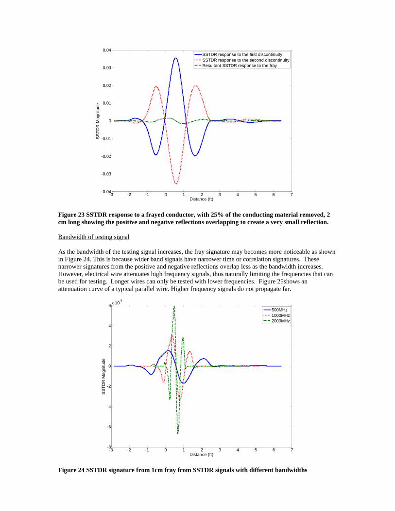
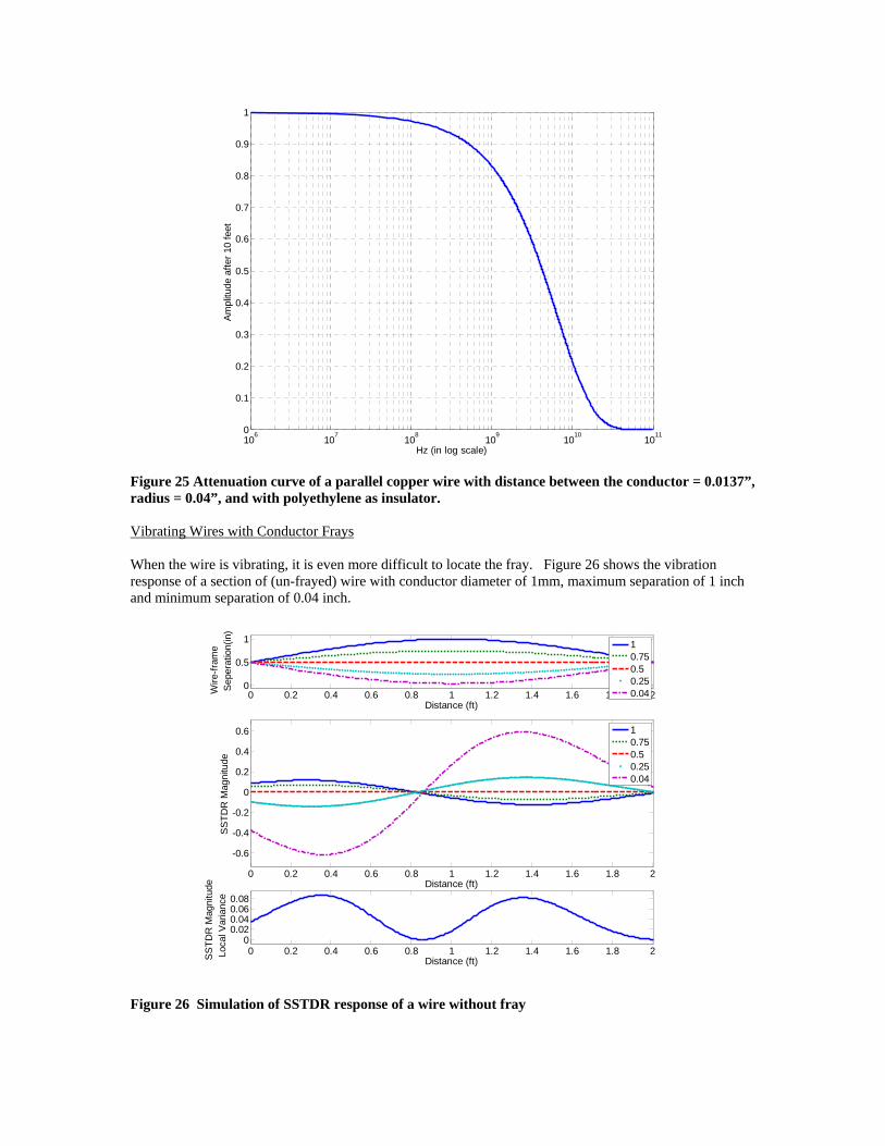
Figure 23 SSTDR response to a frayed conductor, with 25% of the conducting material removed, 2 cm long showing the positive and negative reflections overlapping to create a very small reflection. Bandwidth of testing signal As the bandwidth of the testing signal increases, the fray signature may becomes more noticeable as shown in Figure 24. This is because wider band signals have narrower time or correlation signatures. These narrower signatures from the positive and negative reflections overlap less as the bandwidth increases. However, electrical wire attenuates high frequency signals, thus naturally limiting the frequencies that can be used for testing. Longer wires can only be tested with lower frequencies. Figure 25shows an attenuation curve of a typical parallel wire. Higher frequency signals do not propagate far.

-3 -2 -1 0 1 2 3 4 5 6 7-8

-6

-4

-2

0

2

4

6 x 10-3

Distance (ft)

SS

TDR

Mag

nitu

de

500MHz1000MHz2000MHz

Figure 24 SSTDR signature from 1cm fray from SSTDR signals with different bandwidths

106

107

108

109

1010

10110

0.1

0.2

0.3

0.4

0.5

0.6

0.7

0.8

0.9

1

Am

plitu

de a

fter 1

0 fe

et

Hz (in log scale)

Figure 25 Attenuation curve of a parallel copper wire with distance between the conductor = 0.0137”, radius = 0.04”, and with polyethylene as insulator. Vibrating Wires with Conductor Frays When the wire is vibrating, it is even more difficult to locate the fray. Figure 26 shows the vibration response of a section of (un-frayed) wire with conductor diameter of 1mm, maximum separation of 1 inch and minimum separation of 0.04 inch.

0 0.2 0.4 0.6 0.8 1 1.2 1.4 1.6 1.8 20

0.5

1

Distance (ft)

Wire

-fram

e S

eper

atio

n(in

)

10.750.50.250.04

0 0.2 0.4 0.6 0.8 1 1.2 1.4 1.6 1.8 2

-0.6

-0.4

-0.2

0

0.2

0.4

0.6

Distance (ft)

SS

TDR

Mag

nitu

de

10.750.50.250.04

0 0.2 0.4 0.6 0.8 1 1.2 1.4 1.6 1.8 20

0.020.040.060.08

Distance (ft)SS

TDR

Mag

nitu

de

Loc

al V

aria

nce

Figure 26 Simulation of SSTDR response of a wire without fray

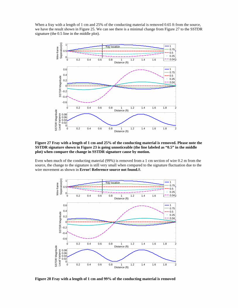
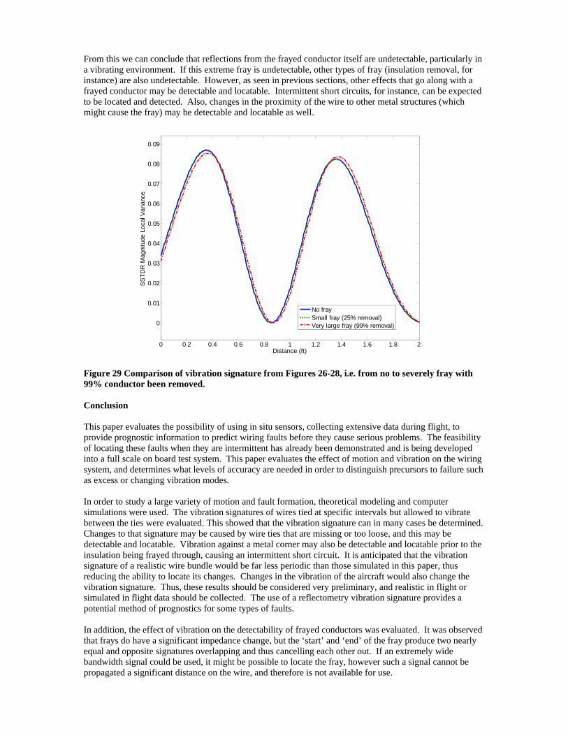
When a fray with a length of 1 cm and 25% of the conducting material is removed 0.65 ft from the source, we have the result shown in Figure 25. We can see there is a minimal change from Figure 27 to the SSTDR signature (the 0.5 line in the middle plot).

0 0.2 0.4 0.6 0.8 1 1.2 1.4 1.6 1.8 20

0.5

1

Distance (ft)

Wire

-fram

e S

eper

atio

n(in

)

10.750.50.250.04

0 0.2 0.4 0.6 0.8 1 1.2 1.4 1.6 1.8 2

-0.6

-0.4

-0.2

0

0.2

0.4

0.6

Distance (ft)

SS

TDR

Mag

nitu

de

10.750.50.250.04

0 0.2 0.4 0.6 0.8 1 1.2 1.4 1.6 1.8 20

0.020.040.060.08

Distance (ft)SS

TDR

Mag

nitu

de

Loc

al V

aria

nce

fray location

Figure 27 Fray with a length of 1 cm and 25% of the conducting material is removed. Please note the SSTDR signature shown in Figure 23 is going unnoticeable (the line labeled as “0.5” in the middle plot) when compare the change in SSTDR signature cause by motion. Even when much of the conducting material (99%) is removed from a 1 cm section of wire 0.2 m from the source, the change to the signature is still very small when compared to the signature fluctuation due to the wire movement as shown in Error! Reference source not found.8.

0 0.2 0.4 0.6 0.8 1 1.2 1.4 1.6 1.8 20

0.5

1

Distance (ft)

Wire

-fram

e S

eper

atio

n(in

)

0 0.2 0.4 0.6 0.8 1 1.2 1.4 1.6 1.8 2

-0.6

-0.4

-0.2

0

0.2

0.4

0.6

Distance (ft)

SS

TDR

Mag

nitu

de

0 0.2 0.4 0.6 0.8 1 1.2 1.4 1.6 1.8 20

0.020.040.060.08

Distance (ft)SS

TDR

Mag

nitu

de

Loc

al V

aria

nce

10.750.50.250.04

10.750.50.250.04

fray location

Figure 28 Fray with a length of 1 cm and 99% of the conducting material is removed

From this we can conclude that reflections from the frayed conductor itself are undetectable, particularly in a vibrating environment. If this extreme fray is undetectable, other types of fray (insulation removal, for instance) are also undetectable. However, as seen in previous sections, other effects that go along with a frayed conductor may be detectable and locatable. Intermittent short circuits, for instance, can be expected to be located and detected. Also, changes in the proximity of the wire to other metal structures (which might cause the fray) may be detectable and locatable as well.

0 0.2 0.4 0.6 0.8 1 1.2 1.4 1.6 1.8 2

0

0.01

0.02

0.03

0.04

0.05

0.06

0.07

0.08

0.09

Distance (ft)

SS

TDR

Mag

nitu

de L

ocal

Var

ianc

e

No fraySmall fray (25% removal)Very large fray (99% removal)

Figure 29 Comparison of vibration signature from Figures 26-28, i.e. from no to severely fray with 99% conductor been removed. Conclusion This paper evaluates the possibility of using in situ sensors, collecting extensive data during flight, to provide prognostic information to predict wiring faults before they cause serious problems. The feasibility of locating these faults when they are intermittent has already been demonstrated and is being developed into a full scale on board test system. This paper evaluates the effect of motion and vibration on the wiring system, and determines what levels of accuracy are needed in order to distinguish precursors to failure such as excess or changing vibration modes. In order to study a large variety of motion and fault formation, theoretical modeling and computer simulations were used. The vibration signatures of wires tied at specific intervals but allowed to vibrate between the ties were evaluated. This showed that the vibration signature can in many cases be determined. Changes to that signature may be caused by wire ties that are missing or too loose, and this may be detectable and locatable. Vibration against a metal corner may also be detectable and locatable prior to the insulation being frayed through, causing an intermittent short circuit. It is anticipated that the vibration signature of a realistic wire bundle would be far less periodic than those simulated in this paper, thus reducing the ability to locate its changes. Changes in the vibration of the aircraft would also change the vibration signature. Thus, these results should be considered very preliminary, and realistic in flight or simulated in flight data should be collected. The use of a reflectometry vibration signature provides a potential method of prognostics for some types of faults. In addition, the effect of vibration on the detectability of frayed conductors was evaluated. It was observed that frays do have a significant impedance change, but the ‘start’ and ‘end’ of the fray produce two nearly equal and opposite signatures overlapping and thus cancelling each other out. If an extremely wide bandwidth signal could be used, it might be possible to locate the fray, however such a signal cannot be propagated a significant distance on the wire, and therefore is not available for use.

The simulations in this paper have shown that vibration-induced reflectometry signatures may provide some prognostic information for mechanical risks for chafing conditions. Additional data must be collected on realistic wiring installations undergoing vibration on order to further assess the feasibility of this method. Acknowledgements This work was supported by the Air Force Research Laboratory. References

[1] J.P. Steiner, W.L. Weeks, Time-Domain Reflectometry for Monitoring Cable Changes: Feasibility Study, EPRI GS-6642, February 1990

[2] Brent Waddoups, Cynthia Furse, Mark Schmidt, Analysis of Reflectometry for Detection of

Chafed Aircraft Wiring Insulation, 5th Joint NASA/FAA/DoD Conference on Aging Aircraft Sept. 10-13, 2001, Orlando, Florida

[3] Brent Waddoups, “Analysis of reflectometry for detection of chafed aircraft wiring insulation.”

Masters Thesis, Utah State University, 2001 (available from http://wwwlib.umi.com/dissertations/)

[4] Alok Jani, “Location of Small Frays using TDR,” Masters Thesis,Utah State University, Logan, Utah, 2003. Available from: ProQuest Information and Learning: (http://wwwlib.umi.com/dissertations/)

[5] Lance Griffiths, Rohit Parakh, Cynthia Furse, Brittany Baker, “The Invisible Fray: A Critical Analysis of the Use of Reflectometry for Fray Location,” IEEE Journal of Sensors, Volume 6, Issue 3, June 2006 Page(s):697 – 70

[6] Cynthia Furse, You Chung Chung, Chet, Lo, Praveen Pendayala, “A Critical Comparison of Reflectometry Methods for Location of Wiring Faults,” Smart Structures and Systems, Vol. 2, No.1, 2006, pp. 25-46

[7] M.N.O. Sadiku, Numerical Techniques in Electromagnetics, CRC Press, 2001

[8] C Lo, C Furse, Modeling and Simulation of Branched Wiring Networks, accepted to Applied Computational Electromagnetics Society Journal

[9] B.C. Wadell, Transmission Line Handbook, Artech House, 1991