Prognostics for Ground Support Systems: Case … for Ground Support Systems: Case Study on Pneumatic Valves Matthew Daigle University of California, Santa Cruz, NASA Ames Research

Prognostics for Ground Support Systems:

Case Study on Pneumatic Valves

Matthew Daigle∗

University of California, Santa Cruz, NASA Ames Research Center, Moffett Field, CA, 94035, USA

Kai Goebel†

NASA Ames Research Center, Moffett Field, CA, 94035, USA

Prognostics technologies determine the health (or damage) state of a component or sub-system, and make end of life (EOL) and remaining useful life (RUL) predictions. Such infor-mation enables system operators to make informed maintenance decisions and streamlineoperational and mission-level activities. We develop a model-based prognostics method-ology for pneumatic valves used in ground support equipment for cryogenic propellantloading operations. These valves are used to control the flow of propellant, so failures mayhave a significant impact on launch availability. Therefore, correctly predicting when valveswill fail enables timely maintenance that avoids launch delays and aborts. The approachutilizes mathematical models describing the underlying physics of valve degradation, and,employing the particle filtering algorithm for joint state-parameter estimation, determinesthe health state of the valve and the rate of damage progression, from which EOL andRUL predictions are made. We develop a prototype user interface for valve prognostics,and demonstrate the prognostics approach using historical pneumatic valve data from theSpace Shuttle refueling system.

Nomenclature

ISHM Integrated Systems Health ManagementEOL end of lifeRUL remaining useful lifeLH2 liquid hydrogent or k timetP or kP time of predictionx state vectorθ parameter vectorv process noise vectory output vectorn measurement noise vectorTEOL EOL thresholdRMAD relative median absolute deviationRA relative accuracy

I. Introduction

Within Integrated Systems Health Management (ISHM), technical advances in and increased acceptanceof automated diagnosis technologies are leading to a shift in research focus to the area of automated prognos-∗Associate Scientist, University of California, Santa Cruz, NASA Ames Research Center, Moffett Field, CA 94035. Member,

AIAA.†Senior Scientist, Prognostics Center of Excellence, NASA Ames Research Center, Moffett Field, CA 94035. Member, AIAA.

1 of 16

American Institute of Aeronautics and Astronautics

https://ntrs.nasa.gov/search.jsp?R=20110012185 2018-07-04T04:02:04+00:00Z

tics. Prognostics algorithms focus on determining the health (or damage) state of a component or subsystem,and making end of life (EOL) and remaining useful life (RUL) predictions. EOL and RUL predictions en-able system operators to make informed maintenance decisions and streamline operational and mission-levelactivities.

As a case study, we consider ground support equipment from the Space Shuttle cryogenic refueling system.This system transfers cryogenic propellants from a storage tank to the vehicle tank through a network ofpipes and valves. Since the valves are used to control the flow of propellant, failures may have a significantimpact on launch availability. Hence, valve prognostics can provide significant value to launch operations.We focus on one of the pneumatic transfer line valves in this system, and apply a model-based prognosticsapproach.

For the selected valve, we develop a complete prognostics solution, including models, algorithms, and auser interface. The prognostics algorithms are model-based, meaning that, unlike data-driven approaches,1

we use mathematical models describing the underlying physical principles of valve operation and how valvesfail.2–6 We construct a detailed physics-based model of a pneumatic valve that includes models of differentdamage mechanisms and how they progress in time. Using this model, we employ the particle filteringalgorithm for joint state-parameter estimation to determine the health state of the valve and the rates ofdamage progression, from which EOL and RUL predictions are made. Although we focus on a pneumaticvalve, the approach is general in that it may be applied to any component, given its model. We also developa prototype user interface to communicate the algorithm results, based on an analysis of what informationthe algorithms provide and how the information should be made available to the user. We demonstrate theprognostics approach as applied to a real-world case study using historical pneumatic valve data from theSpace Shuttle refueling system.

The paper is organized as follows. Section II formulates the prognostics approach. Section III describesthe valve model. Section IV describes the damage estimation algorithm, and Section V describes the pre-diction algorithm. Section VI develops the prognostics interface. Section VII demonstrates the approach onhistorical pneumatic valve data. Section VIII concludes the paper.

II. Prognostics Approach

The goal of prognostics is to predict the EOL and/or the RUL of a component. In this section, we firstformally define the problem of model-based prognostics. We then describe a general model-based architecturewithin which a prognostics solution may be implemented.

II.A. Problem Formulation

We assume the system may be described by

x(t) = f(t,x(t),θ(t),u(t),v(t))y(t) = h(t,x(t),θ(t),u(t),n(t)),

where x(t) ∈ Rnx is the state vector, θ(t) ∈ Rnθ is the parameter vector, u(t) ∈ Rnu is the input vector,v(t) ∈ Rnv is the process noise vector, f is the state equation, y(t) ∈ Rny is the output vector, n(t) ∈ Rnnis the measurement noise vector, and h is the output equation. This form represents a general nonlinearmodel with no restrictions on the functional forms of f or h. Further, the noise terms may be coupled ina nonlinear way with the states and parameters. The parameters θ(t) evolve in an unknown way, but, inpractice, are typically considered to be constant.

Our goal is to predict EOL at a given time point tP using the discrete sequence of observations up totime tP , denoted as y0:tP . EOL is defined as the time point at which the component no longer meets afunctional requirement (e.g., a valve does not open in the required amount of time). This point is expressedthrough a damage threshold, beyond which the component fails to function properly. In general, we mayexpress this threshold as a function of the system state and parameters, TEOL(x(t),θ(t)), which determineswhether EOL has been reached, where

TEOL(x(t),θ(t)) =

{1, if EOL is reached0, otherwise.

2 of 16


Using this function, we can formally define EOL with

EOL(tP ) , arg mint≥tP

TEOL(x(t),θ(t)) = 1,

and RUL with

RUL(tP ) , EOL(tP )− tP .

Due to process noise, measurement noise, and uncertainty in the future inputs of the system, we com-pute a probability distribution of the EOL or RUL, i.e., at time tP , we compute p(EOL(tp)|y0:tP ) and/orp(RUL(tP )|y0:tP ).

II.B. Prognostics Architecture

We adopt a model-based approach that utilizes detailed physics-based models of components and systemsthat include descriptions of how faults evolve in time. These models are parameterized by unknown andpossibly time-varying wear parameters, θ(t). Therefore, our solution to the prognostics problem takes theperspective of joint state-parameter estimation. In discrete time k, we estimate xk and θk, and use theseestimates to predict EOL and RUL when desired.

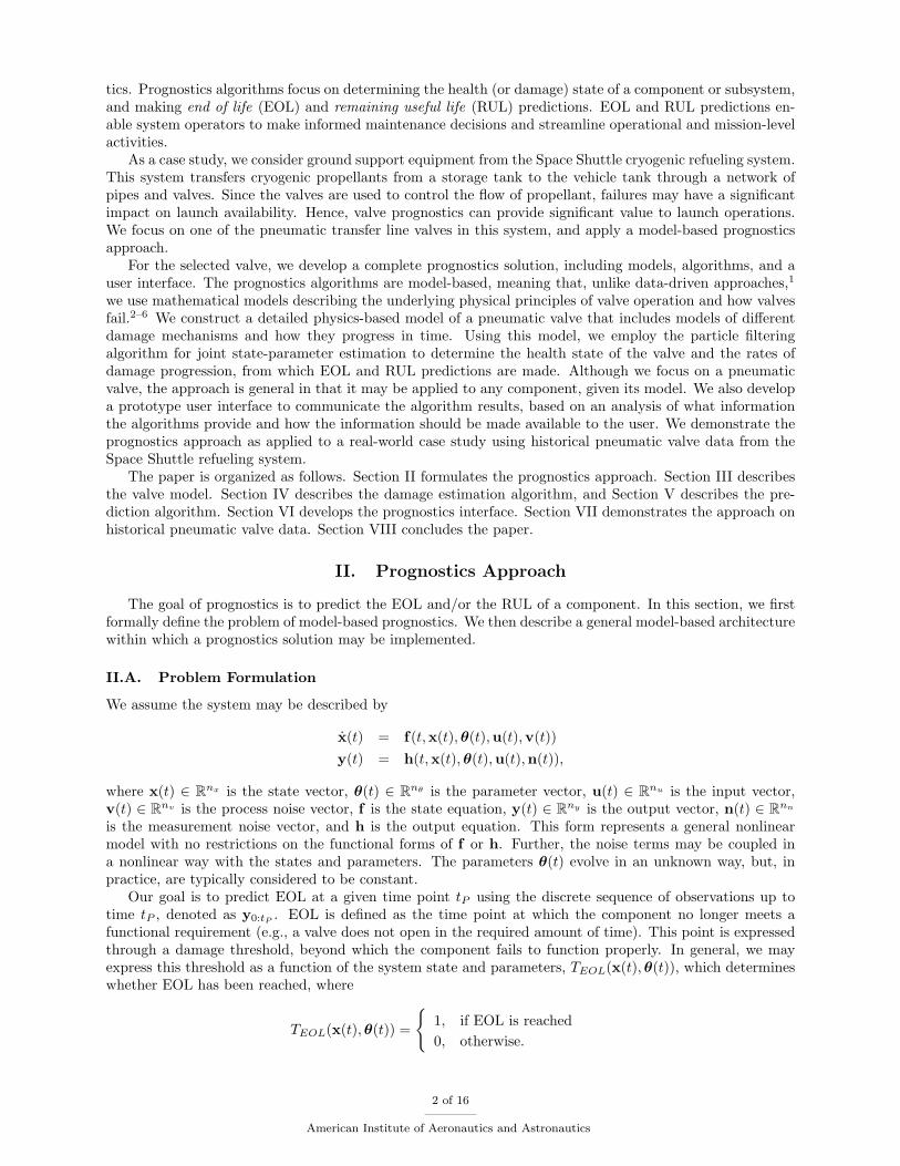
We employ the prognostics architecture in Fig. 1. The system is provided with inputs uk and providesmeasured outputs yk. Prognostics may begin at t = 0, with the damage estimation module determiningestimates of the states and unknown parameters, represented as a probability distribution p(xk,θk|y0:k).The prediction module uses the joint state-parameter distribution, along with hypothesized future inputs, tocompute EOL and RUL as probability distributions p(EOLkP |y0:kP ) and p(RULkP |y0:kP ) at given predictiontimes kP . In parallel, a fault detection, isolation, and identification (FDII) module may be used to determinewhich damage mechanisms are active, represented as a fault set F. The damage estimation module maythen use this result to limit the space of parameters that must be estimated. Alternatively, prognostics maybegin only when diagnostics has completed. In this paper, we focus on the damage estimation and predictionmodules, and begin prognostics at t = 0 without the aid of an FDII solution.

Figure 1. Prognostics architecture.

III. Valve Modeling

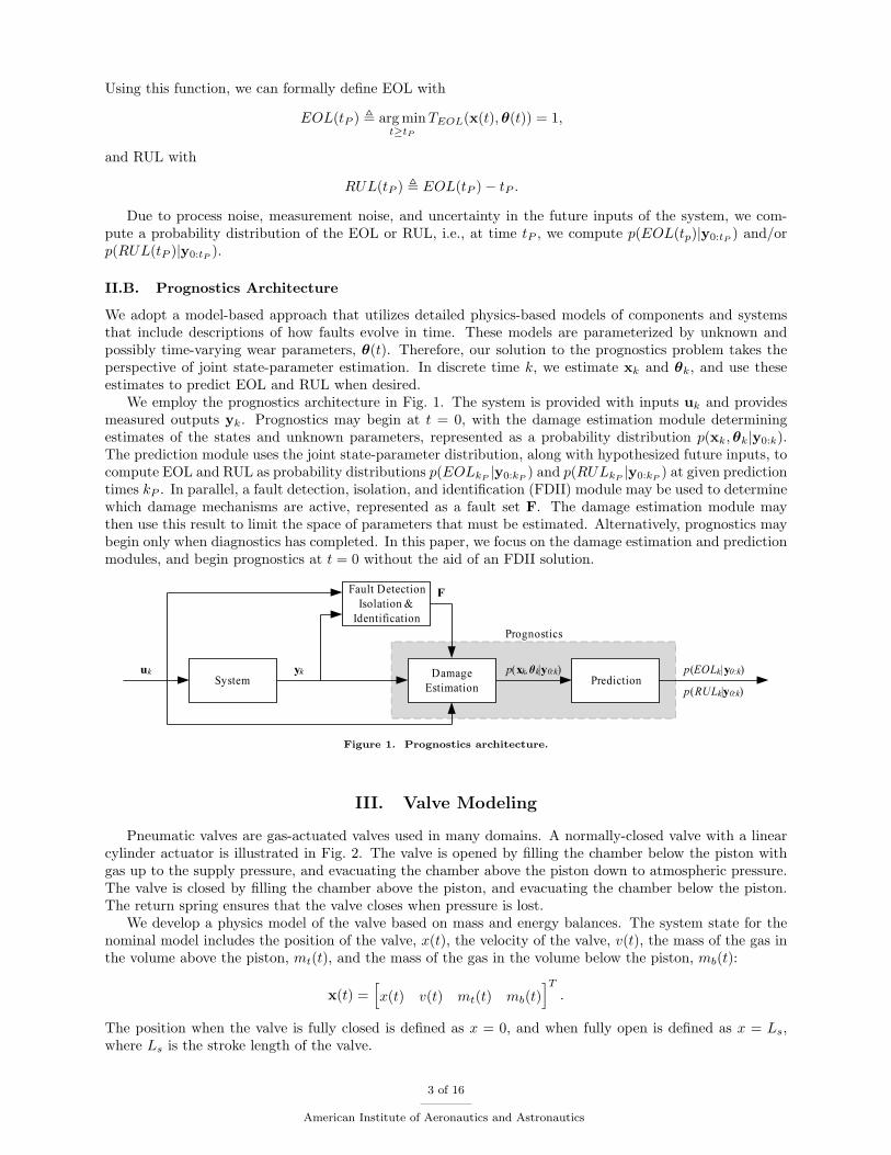
Pneumatic valves are gas-actuated valves used in many domains. A normally-closed valve with a linearcylinder actuator is illustrated in Fig. 2. The valve is opened by filling the chamber below the piston withgas up to the supply pressure, and evacuating the chamber above the piston down to atmospheric pressure.The valve is closed by filling the chamber above the piston, and evacuating the chamber below the piston.The return spring ensures that the valve closes when pressure is lost.

We develop a physics model of the valve based on mass and energy balances. The system state for thenominal model includes the position of the valve, x(t), the velocity of the valve, v(t), the mass of the gas inthe volume above the piston, mt(t), and the mass of the gas in the volume below the piston, mb(t):

x(t) =[x(t) v(t) mt(t) mb(t)

]T.

The position when the valve is fully closed is defined as x = 0, and when fully open is defined as x = Ls,where Ls is the stroke length of the valve.

3 of 16


Figure 2. Pneumatic valve.

The derivatives of the states are described by

x(t) =[v(t) a(t) ft(t) fb(t)

]T,

where a(t) is the valve acceleration, and ft(t) and fb(t) are the mass flows going into the top and bottompneumatic ports, respectively.

The inputs are considered to be

u(t) =[pl(t) pr(t) ut(t) ub(t)

]T,

where pl(t) and pr(t) are the fluid pressures on the left and right side of the plug, respectively, and ut(t)and ub(t) are the input pressures to the top and bottom pneumatic ports, which will alternate between thesupply pressure and atmospheric pressure depending on the commanded valve position.

The acceleration is defined by the combined mass of the piston and plug, m, and the sum of forces actingon the valve, which includes the forces from the pneumatic gas, (pb(t)− pt(t))Ap, where pb(t) and pt(t) arethe gas pressures on the bottom and the top of the piston, respectively, and Ap is the surface area of thepiston; the forces from the fluid flowing through the valve, (pr(t) − pl(t))Av, where Av is the area of thevalve contacting the fluid; the weight of the moving parts of the valve, −mg, where g is the acceleration dueto gravity; the spring force, −k(x(t) − xo), where k is the spring constant and xo is the amount of springcompression when the valve is closed; friction, −rv(t), where r is the coefficient of kinetic friction, and thecontact forces Fc(t) at the boundaries of the valve motion,

Fc(t) =

kc(−x), if x < 0,

0, if 0 ≤ x ≤ Ls,−kc(x− Ls), if x > Ls,

where kc is the (large) spring constant associated with the flexible seals.The pressures pt(t) and pb(t) are calculated as:

pt(t) =mt(t)RgT

Vt0 +Ap(Ls − x(t))

pb(t) =mb(t)RgTVb0 +Apx(t)

where we assume an isothermal process in which the (ideal) gas temperature is constant at T , Rg is the gasconstant for the pneumatic gas, and Vt0 and Vb0 are the minimum gas volumes for the gas chambers aboveand below the piston, respectively.

The gas flows are given by:

ft(t) = fg(pt(t), ut(t))fb(t) = fg(pb(t), ub(t)),

4 of 16


where fg defines gas flow through an orifice for choked and non-choked flow conditions.7 Non-choked flowfor p1 ≥ p2 is given by fg,nc(p1, p2) =

CsAsp1

√γ

ZRgT

(2

γ−1

)((p2p1

) 2γ −

(p2p1

) γ+1γ

),

where γ is the ratio of specific heats, Z is the gas compressibility factor, Cs is the flow coefficient, and As isthe orifice area. Choked flow for p1 ≥ p2, which occurs when p1/p2 exceeds

(γ+1

2

)γ/(γ−1), is given by

fg,c(p1, p2) = CsAsp1

√γ

ZRgT

(2

γ+1

) γ+1γ−1

.

The overall gas flow equation is then given by

fg(p1, p2) =

fg,nc(p1, p2) if p1 ≥ p2 and p1

p2<(γ+1

2

) γ(γ−1) ,

fg,c(p1, p2) if p1 ≥ p2 and p1p2≥(γ+1

2

) γ(γ−1) ,

−fg,nc(p2, p1) if p2 > p1 and p2p1<(γ+1

2

) γ(γ−1) ,

−fg,c(p2, p1) if p2 > p1 and p2p1≥(γ+1

2

) γ(γ−1) ,

.

We select our complete measurement vector as

y(t) =[x(t) pt(t) pb(t) fv(t) open(t) closed(t)

]T,

where fv is the fluid flow through the valve:

fv(t) =x(t)Ls

CvAv

√2ρ |pfl − pfr|sign(pfl − pfr),

Cv is the (dimensionless) flow coefficient of the valve, ρ is the liquid density, and we assume a linear flowcharacteristic for the valve. The open(t) and closed(t) signals are from discrete sensors which output 1 ifthe valve is in the fully opened or fully closed state:

open(t) =

1, if x(t) ≥ Ls0, otherwise

closed(t) =

1, if x(t) ≤ 0

0, otherwise.

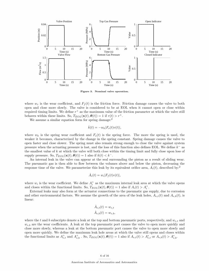
Fig. 3 shows a nominal valve cycle. The valve is commanded to open at 0 s. The top pneumatic portopens to atmosphere and the bottom opens to the supply pressure. When the force on the underside of thepiston is large enough to overcome the opposing forces, the valve begins to move upward as the pneumaticgas continues to flow into and out of the valve actuator. In a little over 1 s, the valve is completely open.The valve is commanded to close at 10 s. The bottom pneumatic port opens to atmosphere and the topopens to the supply pressure. When the force balance becomes negative, the valve starts to move downward,and completely closes within 1 s. The valve closes faster than it opens due to the return spring.

III.A. Damage Modeling

From valve documentation and historical maintenance records, we have identified friction damage, springdamage, internal valve leaks, and external valve leaks as faults that lead to EOL. The variables that describethe magnitude of damage augment the state vector x(t), and the parameters defining their progression formthe unknown parameter vector θ(t).

One damage mechanism present in valves is sliding wear, which results in an increase in friction.8 Wecharacterize friction damage as change in the friction coefficient, and model the damage progression in aform similar to the sliding wear equation:2

r(t) = wr|Ff (t)v(t)|

5 of 16


0 5 10 15 200

0.02

0.04

Posi

tion

(m)

Time (s)

Valve Position

0 5 10 15 200

0.5

1

1.5

Flow

(m

3 /s)

Time (s)

Valve Flow

0 5 10 15 200

2

4

6

Pres

sure

(M

Pa)

Time (s)

Top Gas Pressure

0 5 10 15 200

2

4

6

Pres

sure

(M

Pa)

Time (s)

Bottom Gas Pressure

0 5 10 15 200

0.5

1

Val

ue

Time (s)

Open Indicator

0 5 10 15 200

0.5

1

Val

ue

Time (s)

Closed Indicator

Figure 3. Nominal valve operation.

where wr is the wear coefficient, and Ff (t) is the friction force. Friction damage causes the valve to bothopen and close more slowly. The valve is considered to be at EOL when it cannot open or close withinrequired timing limits. We define r+ as the maximum value of the friction parameter at which the valve stillbehaves within these limits. So, TEOL(x(t),θ(t)) = 1 if r(t) > r+.

We assume a similar equation form for spring damage:2

k(t) = −wk|Fs(t)v(t)|,

where wk is the spring wear coefficient and Fs(t) is the spring force. The more the spring is used, theweaker it becomes, characterized by the change in the spring constant. Spring damage causes the valve toopen faster and close slower. The spring must also remain strong enough to close the valve against systempressure when the actuating pressure is lost, and the loss of this function also defines EOL. We define k− asthe smallest value of k at which the valve will both close within the timing limit and fully close upon loss ofsupply pressure. So, TEOL(x(t),θ(t)) = 1 also if k(t) < k−.

An internal leak in the valve can appear at the seal surrounding the piston as a result of sliding wear.The pneumatic gas is then able to flow between the volumes above and below the piston, decreasing theresponse time of the valve. We parameterize this leak by its equivalent orifice area, Ai(t), described by:2

Ai(t) = wi|Ff (t)v(t)|,

where wi is the wear coefficient. We define A+i as the maximum internal leak area at which the valve opens

and closes within the functional limits. So, TEOL(x(t),θ(t)) = 1 also if Ai(t) > A+i .

External leaks may also form at the actuator connections to the pneumatic gas supply, due to corrosionand other environmental factors. We assume the growth of the area of the leak holes, Ae,t(t) and Ae,b(t), islinear:

Ae,t(t) = we,t

Ae,b(t) = we,b,

where the t and b subscripts denote a leak at the top and bottom pneumatic ports, respectively, and we,t andwe,b are the wear coefficients. A leak at the top pneumatic port causes the valve to open more quickly andclose more slowly, whereas a leak at the bottom pneumatic port causes the valve to open more slowly andopen more quickly. We define the maximum leak hole areas at which the valve still opens and closes withinthe functional limits as A+

e,t and A+e,b . So, TEOL(x(t),θ(t)) = 1 also if Ae,t(t) > A∗e,t or Ae,b(t) > A∗e,b.

6 of 16


Algorithm 1 SIR FilterInputs: {(xik−1,θ

ik−1), w

ik−1}Ni=1,uk−1:k,yk

Outputs: {(xik,θik), wik}Ni=1

for i = 1 to N doθik ∼ p(θk|θik−1)xik ∼ p(xk|xik−1,θ

ik−1,uk−1)

wik ← p(yk|xik,θik,uk)end for

W ←N∑i=1

wik

for i = 1 to N dowik ← wik/W

end for{(xik,θik), wik}Ni=1 ← Resample({(xik,θik), wik}Ni=1)

IV. Damage Estimation

In model-based prognostics, damage estimation is fundamentally a joint state-parameter estimation prob-lem, i.e., computation of p(xk,θk|y0:k).2,3 Particle filters offer a general solution to this problem for non-linear systems with non-Gaussian noise terms,9,10 and have become a favored approach within prognos-tics.2,3, 6, 11,12 As described in Section III, for the pneumatic valves, both the state equation f and theoutput equation h are highly nonlinear, and, further, h contains the discrete measurements open and closed,necessitating the use of particle filters.

In particle filters, the state distribution is approximated by a set of discrete weighted samples, calledparticles. The particle approximation to the state distribution is given by

{(xik,θik), wik}Ni=1,

with N denoting the number of particles. For particle i, xik denotes the state estimates, θik denotes theparameter estimates, and wik denotes the weight. The posterior density is approximated by

p(xk,θk|y0:k) ≈N∑i=1

wikδ(xik,θik)(dxkdθk),

with δ(xik,θik)(dxkdθk) denoting the Dirac delta function located at (xik,θik).

We utilize the sampling importance resampling (SIR) particle filter, given as Algorithm 1. Each particleis propagated forward to time k by sampling new parameter and state values. The particle weight is assignedusing yk. The weights are then normalized, and then the particles are resampled, e.g., using the systematicresampling algorithm.13

The parameters θk evolve by some unknown random process that is independent of the state xk. Toperform parameter estimation within a particle filter framework, we assign a random walk evolution, i.e., forparameter θ, θk = θk−1 +ξk−1, where ξk−1 is a noise term. During the sampling step, particles are generatedwith parameter values that will be different from the current values of the parameters. The particles withparameter values closest to the true values should match the outputs better, and therefore be assignedhigher weight. Resampling will cause more particles to be generated with similar values. The particle filterconverges to the true values as the process is repeated over each step of the algorithm.

The selected variance of the random walk noise determines both the rate of this convergence and theestimation performance once convergence is achieved. Therefore, this parameter should be tuned to obtainthe best possible performance, but the optimal value is dependent on the value of the hidden wear parameter,which is unknown. We use the variance control method presented in Ref. 6, shown as Algorithm 2. In thisapproach, the variance of the hidden wear parameter estimate is controlled to a user-specified range bymodifying the random walk noise variance. We assume that the ξ values are tuned initially based on themaximum expected wear rates. The algorithm uses relative median absolute deviation (RMAD) as themeasure of spread, defined as:

RMAD(X) = 100Mediani (|Xi −Medianj(Xj)|)

Medianj(Xj),

7 of 16


Algorithm 2 ξ AdaptationInputs: {(xik,θik), wik}Ni=1, ξk−1

State: aOutputs: ξkif k = 0 then

a← 0end iffor all j ∈ {1, 2, . . . , nθ} dovj ← RMAD({θik(j)}Ni=1)if a(j) = 0 and vj < T then

a(j)← 1end ifif a(j) = 0 thenv∗j ← v∗j0

elsev∗j ← v∗j∞

end ifξk(j)← ξk−1(j)

(1 + P

vj−v∗jv∗j

)end for

where X is a data set and Xi is an element of that set. The adaptation scheme resembles a proportionalcontrol law, where the error between the actual RMAD of a parameter θ(j), denoted as vj in the algorithm,and the desired RMAD value (e.g., 10%), denoted as v∗j in the algorithm, is normalized by vj . The error isthen multiplied by a factor P (e.g., 1× 10−3), and the corresponding variance ξ(j) is increased or decreasedby that percentage. There are two different setpoints. First, we allow for a convergence period, with setpointv∗j0 (e.g., 50%). Once vj reaches T (e.g., 1.2v∗j0), we mark it using the a(j) flag, and begin to control it to anew setpoint v∗j∞ (e.g., 10%).

V. Prediction

Prediction is initiated at a given time kP . Using the current state estimate, p(xk,θk|y0:k) the goal is tocompute p(EOLkP |y0:kP ) and p(RULkP |y0:kP ). The particle filter computes

p(xkP ,θkP |y0:kP ) ≈N∑i=1

wikP δ(xikP ,θikP

)(dxkP dθkP ).

We can approximate a prediction distribution n steps forward as14

p(xkP+n,θkP+n|y0:kP ) ≈N∑i=1

wikP δ(xikP+n,θikP+n)(dxkP+ndθkP+n).

So, for a particle i propagated n steps forward without new data, we can simply take its weight as wikP .Similarly, we can approximate the EOL as

p(EOLkP |y0:kP ) ≈N∑i=1

wikP δEOLikP(dEOLkP ).

To compute EOL, then, we propagate each particle forward to its own EOL and use that particle’s weightat kP for the weight of its EOL prediction.

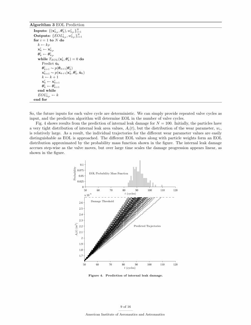
The pseudocode for the prediction procedure is given as Algorithm 3.2 Each particle i is propagatedforward until TEOL(xik,θ

ik) evaluates to 1, at this point EOL has been reached for this particle. Prediction

requires hypothesizing future inputs of the system, uk. For the valve, this problem is simplified, becauseeach valve cycle corresponds to the same set of inputs, because the fluid pressures pL and pR can safely beassumed to be constant in our application domain, and, further, have an almost negligible effect on valvebehavior because the forces they produce are very small compared to the other forces acting on the valve.

8 of 16


Algorithm 3 EOL PredictionInputs: {(xikP ,θ

ik), w

ikP}Ni=1

Outputs: {EOLikP , wikP}Ni=1

for i = 1 to N dok ← kPxik ← xikPθik ← θikPwhile TEOL(xik,θ

ik) = 0 do

Predict ukθik+1 ∼ p(θk+1|θik)xik+1 ∼ p(xk+1|xik,θik, uk)k ← k + 1xik ← xik+1

θik ← θik+1

end whileEOLikP ← k

end for

So, the future inputs for each valve cycle are deterministic. We can simply provide repeated valve cycles asinput, and the prediction algorithm will determine EOL in the number of valve cycles.

Fig. 4 shows results from the prediction of internal leak damage for N = 100. Initially, the particles havea very tight distribution of internal leak area values, Ai(t), but the distribution of the wear parameter, wi,is relatively large. As a result, the individual trajectories for the different wear parameter values are easilydistinguishable as EOL is approached. The different EOL values along with particle weights form an EOLdistribution approximated by the probability mass function shown in the figure. The internal leak damageaccrues step-wise as the valve moves, but over large time scales the damage progression appears linear, asshown in the figure.

t (cycles)

Pro

babi

lity

EOL Probability Mass Function

50 60 70 80 90 100 110 1200

0.025

0.05

0.075

0.1

50 60 70 80 90 100 110 120

1.7

1.8

1.9

2

2.1

2.2

2.3

2.4

2.5

2.6

x 10−6

Ai(

t)(m

2)

t (cycles)

Damage Threshold

Predicted Trajectories

Figure 4. Prediction of internal leak damage.

9 of 16


VI. Prognostics Interface Design

Since prognostics is still a nascent field, there are no real examples of successful prognostics interfaces.Therefore, in this section, we try to establish some fundamental guidelines and principles for the design ofprognostics interfaces, based on our experience developing a prototype interface for our case study. We firstdescribe the information available from prognostics algorithms that may be presented to a user, then providesome design guidelines, followed by a description of the interface we designed.

VI.A. Information Provided by Prognostics

A prognostics interface must present the results of prognostics algorithms to a user and allow the user tointeract with the algorithm to obtain additional results, view information in a variety of ways, and accesslong-term historical information. In contrast to most systems interfaces, e.g. diagnostics interfaces, in whichinformation is viewed only over short time scales, such as the duration of a mission, prognostics interfacescope with information over very large time scales, such as sequences of missions. Therefore it is important todistinguish these two time scales clearly. Further, it is more useful to an operator for results to be presentedin an operational or missions context, e.g., how many missions a component will survive as opposed to howmuch time or how many cycles it will last.

Prognostics algorithms are capable of presenting a wealth of information to the user. Foremost, algorithmsgenerate predictions of EOL and RUL, i.e., p(EOL(kp)|y0:kP ) and/or p(RUL(kP )|y0:kP ) at given predictiontimes kp. Predictions may be computed automatically by the algorithm, but also on request from a user.As described in Section IV, model-based prognostics algorithms also compute supportive information, suchas state and parameter estimates, p(xk,θk|y0:k), which includes estimates of the amount of damage and therates of damage progression.

As shown in Algorithm 3, the state estimates are used directly to compute EOL. Using the same basicprocedure, other predictions can be made as well, which may be useful to the user. Future state, parameter,and output trajectories can be computed and displayed to the user, which can show how the componentis expected to perform in the future, and how damage is expected to progress. Note also that a numberof health or damage indices may be computed from the state estimates, e.g., that a valve is at 50% healthor its spring is at 75% health. Therefore, predictions of these health indices may also be obtained fromthe predictions of the state trajectories. This type of information is useful to the user because it helps inunderstanding the EOL and RUL predictions made by the algorithm.

Once a component has failed, and ground truth is hence known, the outputs of the algorithm over thelife of the component can be used to evaluate the performance of the algorithm. Various offline performancemetrics may be used for this purpose, such as relative accuracy, convergence, prognostics horizon, and α-λperformance.15 This higher-level information is also beneficial to a system operator.

VI.B. Design Guidelines for a Prognostics Interface

With the wealth of information available from prognostics algorithms, a prognostics interface must avoidoverwhelming the user with too much technical information. In the early life of a component, prognostics isnot a concern, so the interface should indicate when damage has reached a threshold where EOL predictionsbecome relevant so that the user knows when to start viewing the algorithm results. The most criticalinformation, which should be displayed most prominently, includes overall component health and the lifepredictions. The predicted values should be shown over a large time window, so that users can see how theRUL and EOL predictions have evolved in time. Because it takes time for prognostics algorithms to converge,the interface should distinguish between predictions obtained before and after algorithm convergence, sincethe results before convergence are unreliable.

State, parameter, and output estimates provide additional supportive information that helps the userto understand the current life predictions made by the algorithm. In particular, the evolution of damagestates (e.g., spring rate or leakage area) over time demonstrate how the component is degrading, especiallywhen shown against damage limits. It is equally important to show damage as it manifests in the functionalperformance of the component. For example, with the valves, EOL is largely defined by valve openingand closing times, so showing the progression of these values over time against the functional limits is alsouseful. Since damage often manifests as nonlinear changes in the system outputs over time (e.g., exponential

10 of 16


degradation), showing the predicted future output values helps the user understand the connection betweenfunctional performance and the life predictions with additional clarity.

Since most prognostics algorithms provide results as probability distributions, there are multiple waysto view the results. Histograms or probability density functions can be shown, as well as box plots, orthe life predictions at specified confidence levels. The choice of how to display the distribution dependson the type of reasoning that the user is performing. It is then also useful to show summary statisticsfor the various distributions, including measures of central tendency and statistical dispersion, as well ashigher-order moments such as skew and kurtosis.

Besides choosing how information should be displayed, the user may also interact directly with thealgorithm by setting assumptions about the future inputs of the component. For example, a user may beinterested only in worst-case performance, so will assume maximum loading on the component. Instead, auser may be interested in average performance over a distribution of possible future loading profiles. Eachof these cases should be made available to the user.

VI.C. Valve Prognostics Interface

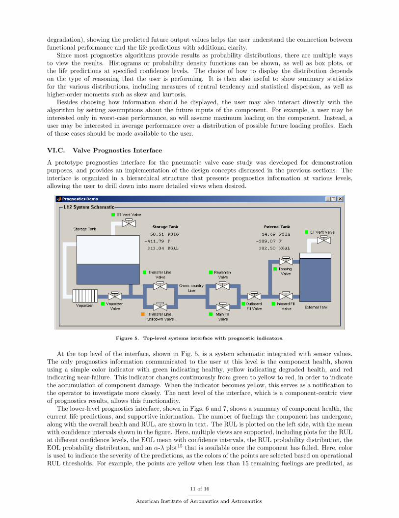
A prototype prognostics interface for the pneumatic valve case study was developed for demonstrationpurposes, and provides an implementation of the design concepts discussed in the previous sections. Theinterface is organized in a hierarchical structure that presents prognostics information at various levels,allowing the user to drill down into more detailed views when desired.

Figure 5. Top-level systems interface with prognostic indicators.

At the top level of the interface, shown in Fig. 5, is a system schematic integrated with sensor values.The only prognostics information communicated to the user at this level is the component health, shownusing a simple color indicator with green indicating healthy, yellow indicating degraded health, and redindicating near-failure. This indicator changes continuously from green to yellow to red, in order to indicatethe accumulation of component damage. When the indicator becomes yellow, this serves as a notification tothe operator to investigate more closely. The next level of the interface, which is a component-centric viewof prognostics results, allows this functionality.

The lower-level prognostics interface, shown in Figs. 6 and 7, shows a summary of component health, thecurrent life predictions, and supportive information. The number of fuelings the component has undergone,along with the overall health and RUL, are shown in text. The RUL is plotted on the left side, with the meanwith confidence intervals shown in the figure. Here, multiple views are supported, including plots for the RULat different confidence levels, the EOL mean with confidence intervals, the RUL probability distribution, theEOL probability distribution, and an α-λ plot15 that is available once the component has failed. Here, coloris used to indicate the severity of the predictions, as the colors of the points are selected based on operationalRUL thresholds. For example, the points are yellow when less than 15 remaining fuelings are predicted, as

11 of 16


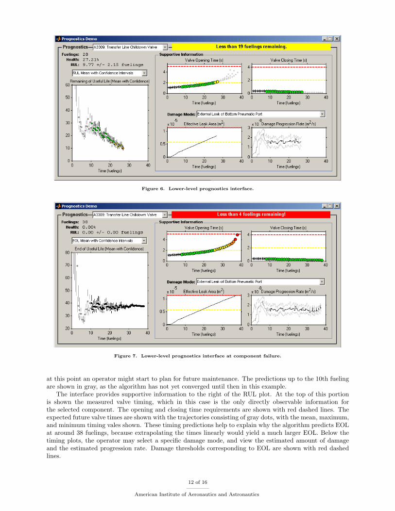
Figure 6. Lower-level prognostics interface.

Figure 7. Lower-level prognostics interface at component failure.

at this point an operator might start to plan for future maintenance. The predictions up to the 10th fuelingare shown in gray, as the algorithm has not yet converged until then in this example.

The interface provides supportive information to the right of the RUL plot. At the top of this portionis shown the measured valve timing, which in this case is the only directly observable information forthe selected component. The opening and closing time requirements are shown with red dashed lines. Theexpected future valve times are shown with the trajectories consisting of gray dots, with the mean, maximum,and minimum timing vales shown. These timing predictions help to explain why the algorithm predicts EOLat around 38 fuelings, because extrapolating the times linearly would yield a much larger EOL. Below thetiming plots, the operator may select a specific damage mode, and view the estimated amount of damageand the estimated progression rate. Damage thresholds corresponding to EOL are shown with red dashedlines.

12 of 16


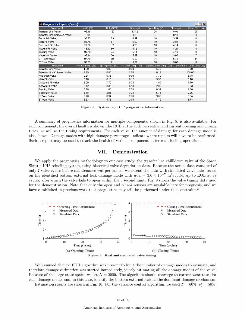
Figure 8. System report of prognostics information.

A summary of prognostics information for multiple components, shown in Fig. 8, is also available. Foreach component, the overall health is shown, the RUL at the 95th percentile, and current opening and closingtimes, as well as the timing requirements. For each valve, the amount of damage for each damage mode isalso shown. Damage modes with high damage percentages indicate where repairs will have to be performed.Such a report may be used to track the health of various components after each fueling operation.

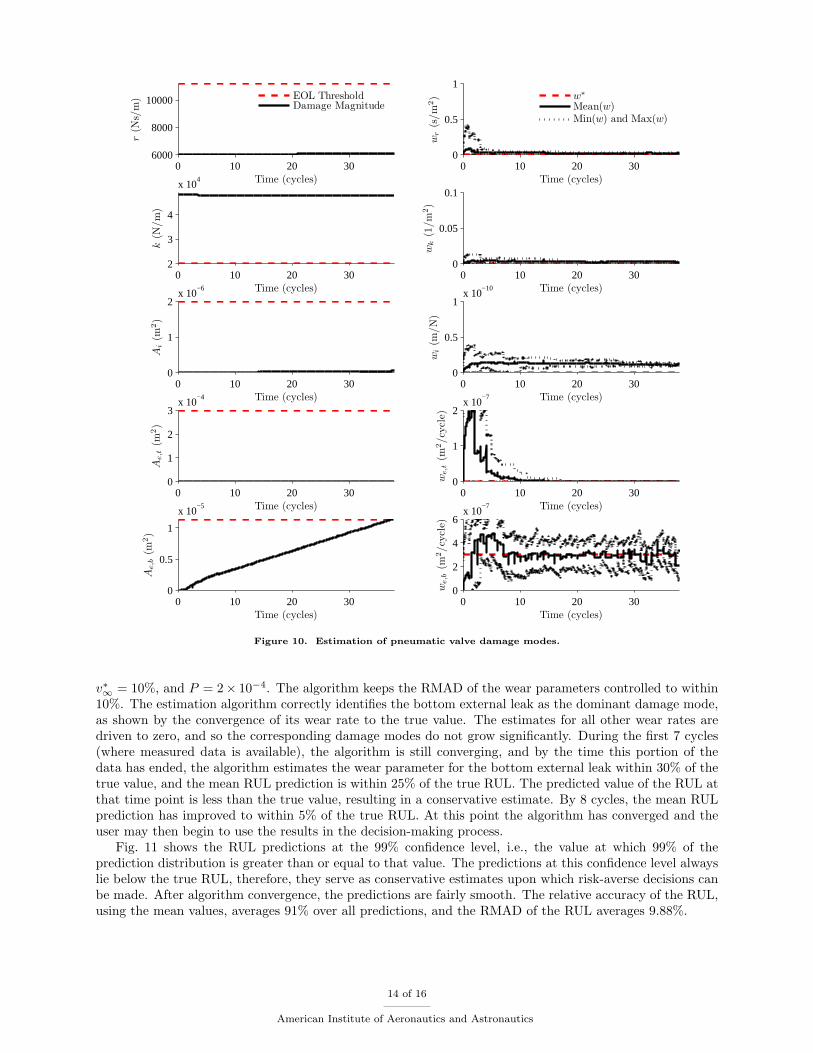
VII. Demonstration

We apply the prognostics methodology to our case study, the transfer line chillldown valve of the SpaceShuttle LH2 refueling system, using historical valve degradation data. Because the actual data consisted ofonly 7 valve cycles before maintenance was performed, we extend the data with simulated valve data, basedon the identified bottom external leak damage mode with we.b = 3.0 × 10−7 m2/cycle, up to EOL at 38cycles, after which the valve fails to open within the 5 second limit. Fig. 9 shows the valve timing data usedfor the demonstration. Note that only the open and closed sensors are available here for prognosis, and wehave established in previous work that prognostics may still be performed under this constraint.2

0 10 20 30 401

2

3

4

5

Time (cycles)

Tim

e (s

)

Opening Time RequirementMeasured DataSimulated Data

(a) Opening Times

0 10 20 30 400

1

2

3

4

Time (cycles)

Tim

e (s

)

Closing Time RequirementMeasured DataSimulated Data

(b) Closing Times

Figure 9. Real and simulated valve timing.

We assumed that no FDII algorithm was present to limit the number of damage modes to estimate, andtherefore damage estimation was started immediately, jointly estimating all the damage modes of the valve.Because of the large state space, we set N = 2000. The algorithm should converge to correct wear rates foreach damage mode, and, in this case, identify the bottom external leak as the dominant damage mechanism.

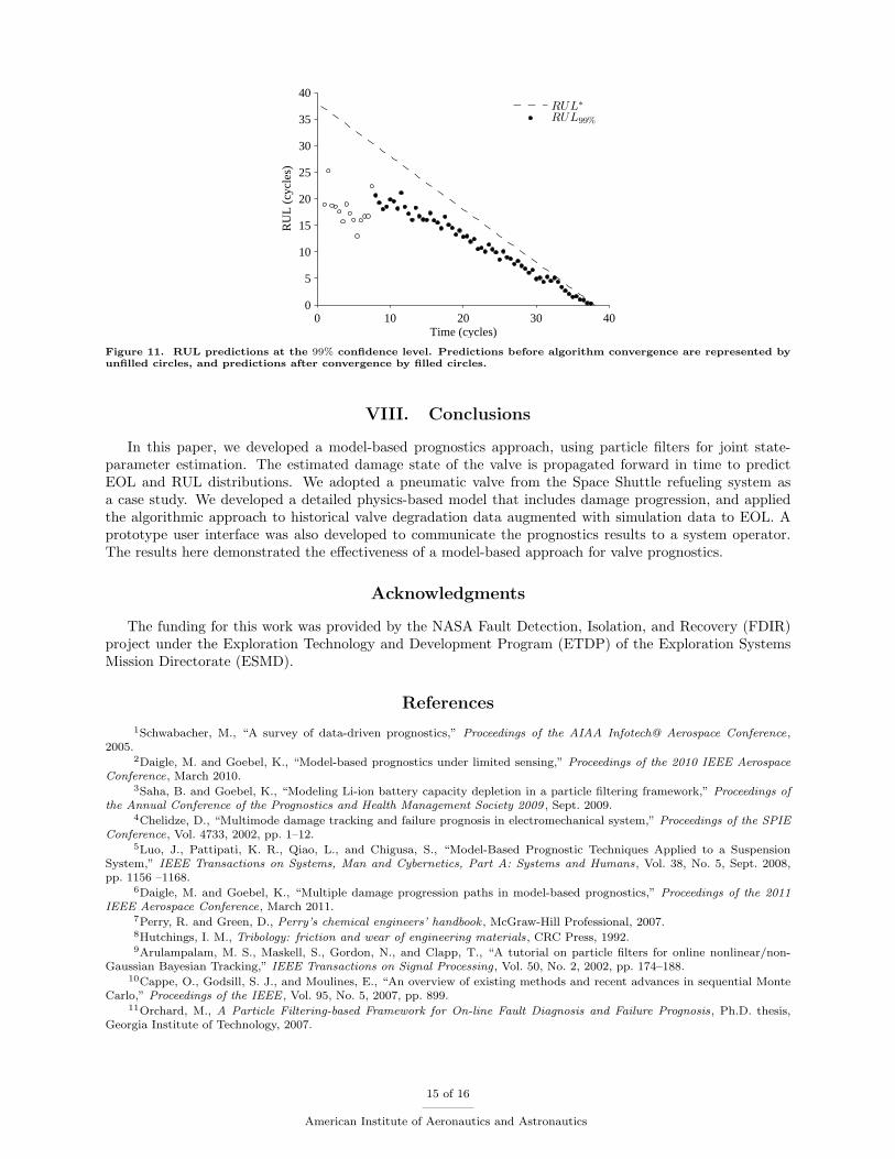
Estimation results are shown in Fig. 10. For the variance control algorithm, we used T = 60%, v∗0 = 50%,

13 of 16


0 10 20 306000

8000

10000

Time (cycles)

r(N

s/m

)

EOL ThresholdDamage Magnitude

0 10 20 300

0.5

1

Time (cycles)

wr

(s/m

2)

w∗Mean(w)Min(w) and Max(w)

0 10 20 302

3

4

x 104

Time (cycles)

k(N

/m)

0 10 20 300

0.05

0.1

Time (cycles)

wk

(1/m

2)

0 10 20 300

1

2x 10

−6

Time (cycles)

Ai

(m2)

0 10 20 300

0.5

1x 10

−10

Time (cycles)

wi(m

/N)

0 10 20 300

1

2

3x 10

−4

Time (cycles)

Ae,t

(m2)

0 10 20 300

1

2x 10

−7

Time (cycles)

we,t

(m2/c

ycle

)

0 10 20 300

0.5

1

x 10−5

Time (cycles)

Ae,b

(m2)

0 10 20 300

2

4

6x 10

−7

Time (cycles)

we,b

(m2/c

ycle

)

Figure 10. Estimation of pneumatic valve damage modes.

v∗∞ = 10%, and P = 2× 10−4. The algorithm keeps the RMAD of the wear parameters controlled to within10%. The estimation algorithm correctly identifies the bottom external leak as the dominant damage mode,as shown by the convergence of its wear rate to the true value. The estimates for all other wear rates aredriven to zero, and so the corresponding damage modes do not grow significantly. During the first 7 cycles(where measured data is available), the algorithm is still converging, and by the time this portion of thedata has ended, the algorithm estimates the wear parameter for the bottom external leak within 30% of thetrue value, and the mean RUL prediction is within 25% of the true RUL. The predicted value of the RUL atthat time point is less than the true value, resulting in a conservative estimate. By 8 cycles, the mean RULprediction has improved to within 5% of the true RUL. At this point the algorithm has converged and theuser may then begin to use the results in the decision-making process.

Fig. 11 shows the RUL predictions at the 99% confidence level, i.e., the value at which 99% of theprediction distribution is greater than or equal to that value. The predictions at this confidence level alwayslie below the true RUL, therefore, they serve as conservative estimates upon which risk-averse decisions canbe made. After algorithm convergence, the predictions are fairly smooth. The relative accuracy of the RUL,using the mean values, averages 91% over all predictions, and the RMAD of the RUL averages 9.88%.

14 of 16


0 10 20 30 400

5

10

15

20

25

30

35

40

Time (cycles)

RU

L (

cycl

es)

RUL∗RUL99%

Figure 11. RUL predictions at the 99% confidence level. Predictions before algorithm convergence are represented byunfilled circles, and predictions after convergence by filled circles.

VIII. Conclusions

In this paper, we developed a model-based prognostics approach, using particle filters for joint state-parameter estimation. The estimated damage state of the valve is propagated forward in time to predictEOL and RUL distributions. We adopted a pneumatic valve from the Space Shuttle refueling system asa case study. We developed a detailed physics-based model that includes damage progression, and appliedthe algorithmic approach to historical valve degradation data augmented with simulation data to EOL. Aprototype user interface was also developed to communicate the prognostics results to a system operator.The results here demonstrated the effectiveness of a model-based approach for valve prognostics.

Acknowledgments

The funding for this work was provided by the NASA Fault Detection, Isolation, and Recovery (FDIR)project under the Exploration Technology and Development Program (ETDP) of the Exploration SystemsMission Directorate (ESMD).

References

1Schwabacher, M., “A survey of data-driven prognostics,” Proceedings of the AIAA Infotech@ Aerospace Conference,2005.

2Daigle, M. and Goebel, K., “Model-based prognostics under limited sensing,” Proceedings of the 2010 IEEE AerospaceConference, March 2010.

3Saha, B. and Goebel, K., “Modeling Li-ion battery capacity depletion in a particle filtering framework,” Proceedings ofthe Annual Conference of the Prognostics and Health Management Society 2009 , Sept. 2009.

4Chelidze, D., “Multimode damage tracking and failure prognosis in electromechanical system,” Proceedings of the SPIEConference, Vol. 4733, 2002, pp. 1–12.

5Luo, J., Pattipati, K. R., Qiao, L., and Chigusa, S., “Model-Based Prognostic Techniques Applied to a SuspensionSystem,” IEEE Transactions on Systems, Man and Cybernetics, Part A: Systems and Humans, Vol. 38, No. 5, Sept. 2008,pp. 1156 –1168.

6Daigle, M. and Goebel, K., “Multiple damage progression paths in model-based prognostics,” Proceedings of the 2011IEEE Aerospace Conference, March 2011.

7Perry, R. and Green, D., Perry’s chemical engineers’ handbook , McGraw-Hill Professional, 2007.8Hutchings, I. M., Tribology: friction and wear of engineering materials, CRC Press, 1992.9Arulampalam, M. S., Maskell, S., Gordon, N., and Clapp, T., “A tutorial on particle filters for online nonlinear/non-

Gaussian Bayesian Tracking,” IEEE Transactions on Signal Processing, Vol. 50, No. 2, 2002, pp. 174–188.10Cappe, O., Godsill, S. J., and Moulines, E., “An overview of existing methods and recent advances in sequential Monte

Carlo,” Proceedings of the IEEE , Vol. 95, No. 5, 2007, pp. 899.11Orchard, M., A Particle Filtering-based Framework for On-line Fault Diagnosis and Failure Prognosis, Ph.D. thesis,

Georgia Institute of Technology, 2007.

15 of 16


12Daigle, M. and Goebel, K., “Model-based prognostics with fixed-lag particle filters,” Proceedings of the Annual Conferenceof the Prognostics and Health Management Society 2009 , Sept. 2009.

13Kitagawa, G., “Monte Carlo filter and smoother for non-Gaussian nonlinear state space models,” Journal of Computa-tional and Graphical Statistics, Vol. 5, No. 1, 1996, pp. 1–25.

14Doucet, A., Godsill, S., and Andrieu, C., “On sequential Monte Carlo sampling methods for Bayesian filtering,” Statisticsand Computing, Vol. 10, 2000, pp. 197–208.

15Saxena, A., Celaya, J., Saha, B., Saha, S., and Goebel, K., “Metrics for Offline Evaluation of Prognostic Performance,”International Journal of Prognostics and Health Management (IJPHM), Vol. 1, 2010.

16 of 16


Documents

Prognostics for Ground Support Systems: Case … for Ground Support Systems: Case Study on Pneumatic Valves Matthew Daigle University of California, Santa Cruz, NASA Ames Research