Embed Size (px)
Citation preview
• 7/28/08
• 1
Program Analysis
Readings • Notes on Representation and Analysis of
Software (Sections 1--5)
• The Program Dependence Graph and Its Use in Optimization
• Dragon book

• 7/28/08
• 2
Program Analysis
Control-flow Analysis
Control Flow: Basic Blocks
• Basic block: a sequence of consecutive statements in which flow of control enters at the beginning and leaves at the end without halt of possibility of branch except at the end
• A basic block may or may not be maximal
• 7/28/08
• 3
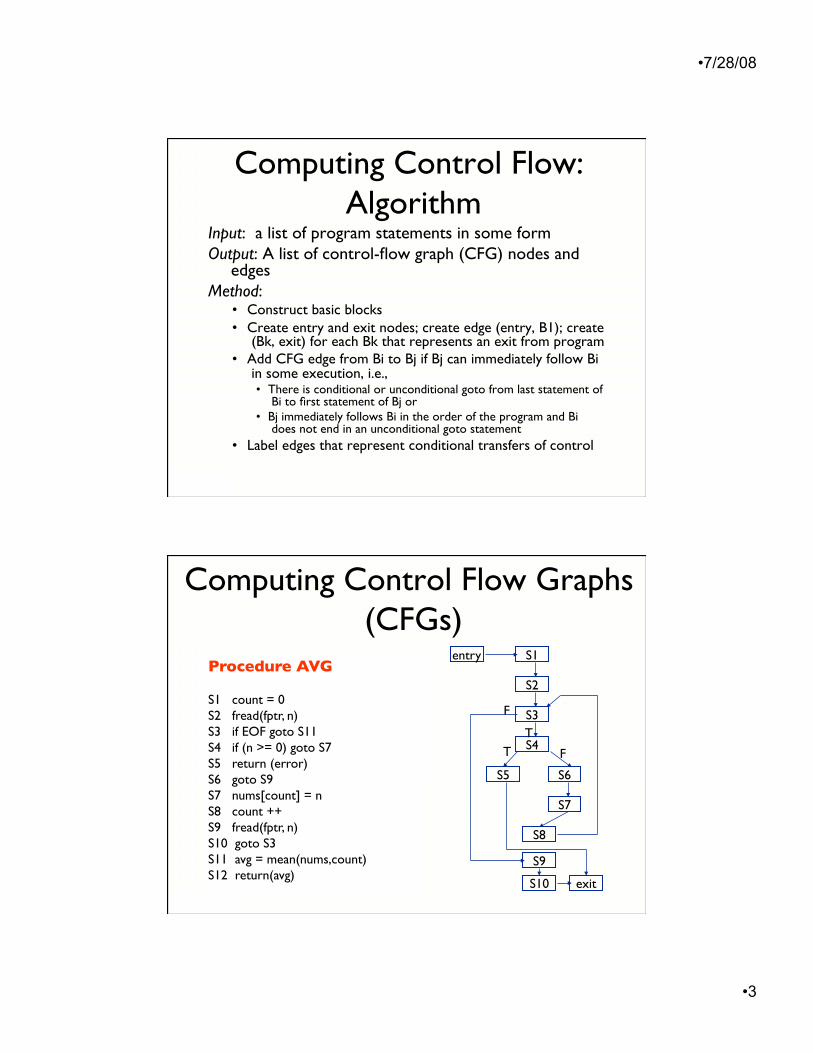
Computing Control Flow: Algorithm
Input: a list of program statements in some form Output: A list of control-flow graph (CFG) nodes and
edges Method:
• Construct basic blocks • Create entry and exit nodes; create edge (entry, B1); create
(Bk, exit) for each Bk that represents an exit from program • Add CFG edge from Bi to Bj if Bj can immediately follow Bi
in some execution, i.e., • There is conditional or unconditional goto from last statement of
Bi to first statement of Bj or • Bj immediately follows Bi in the order of the program and Bi
does not end in an unconditional goto statement • Label edges that represent conditional transfers of control
Computing Control Flow Graphs (CFGs)
Procedure AVG
S1 count = 0 S2 fread(fptr, n) S3 while (not EOF) do S4 if (n < 0) S5 return (error) else S6 nums[count] = n S7 count ++ endif S8 fread(fptr, n) endwhile S9 avg = mean(nums,count) S10 return(avg)
S1
S2
S3
S4
S5 S6
S7
S8
S9
S10
entry
exit
F
T
F
T
Procedure AVG
S1 count = 0 S2 fread(fptr, n) S3 if EOF goto S11 S4 if (n >= 0) goto S7 S5 return (error) S6 goto S9 S7 nums[count] = n S8 count ++ S9 fread(fptr, n) S10 goto S3 S11 avg = mean(nums,count) S12 return(avg)
• 7/28/08
• 4
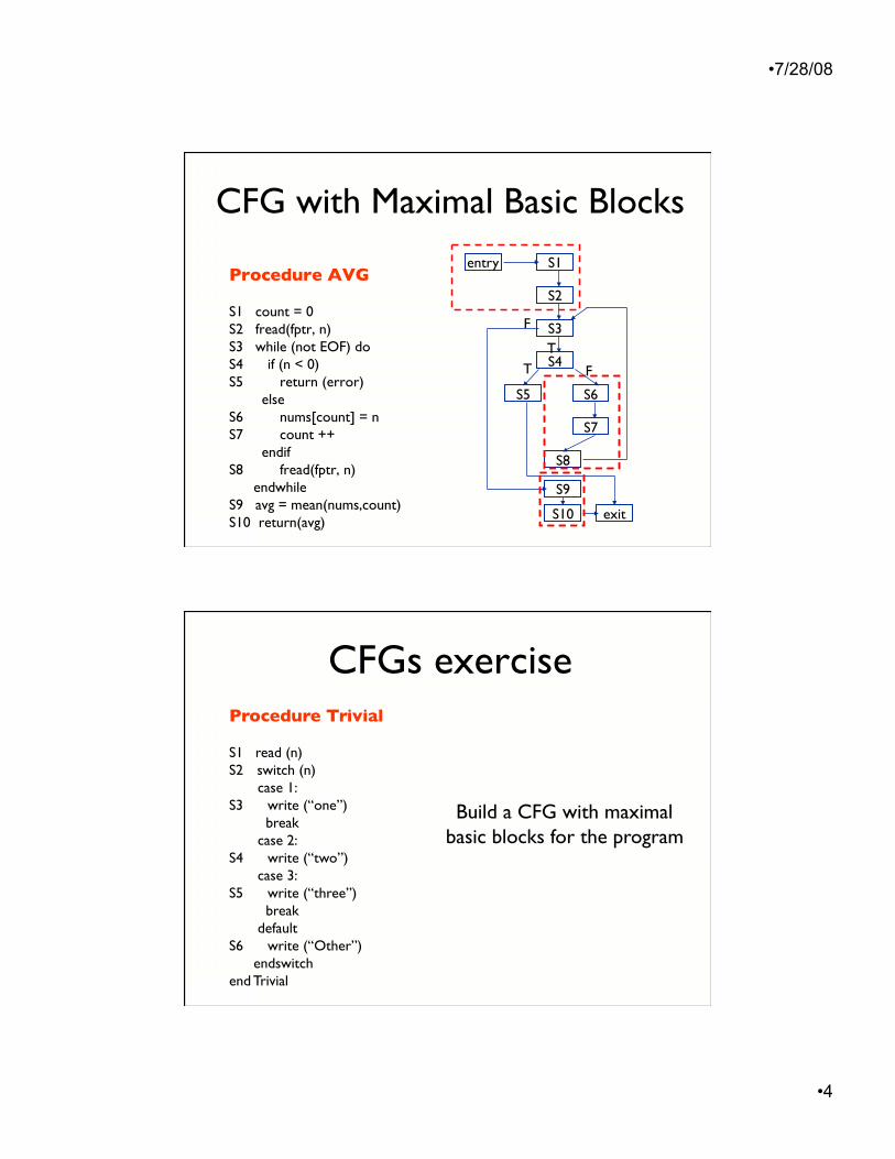
CFG with Maximal Basic Blocks
S1
S2
S3
S4
S5 S6
S7
S8
S9
S10
entry
exit
F
T
F
T
Procedure AVG
S1 count = 0 S2 fread(fptr, n) S3 while (not EOF) do S4 if (n < 0) S5 return (error) else S6 nums[count] = n S7 count ++ endif S8 fread(fptr, n) endwhile S9 avg = mean(nums,count) S10 return(avg)
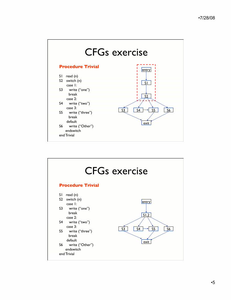
CFGs exercise Procedure Trivial
S1 read (n) S2 switch (n) case 1: S3 write (“one”) break case 2: S4 write (“two”) case 3: S5 write (“three”) break default S6 write (“Other”) endswitch end Trivial
Build a CFG with maximal�basic blocks for the program
• 7/28/08
• 5
CFGs exercise
S1
S2
S3 S4 S5 S6
entry
exit
Procedure Trivial
S1 read (n) S2 switch (n) case 1: S3 write (“one”) break case 2: S4 write (“two”) case 3: S5 write (“three”) break default S6 write (“Other”) endswitch end Trivial
CFGs exercise
entry
S1,2
S3 S4 S5 S6
exit
Procedure Trivial
S1 read (n) S2 switch (n) case 1: S3 write (“one”) break case 2: S4 write (“two”) case 3: S5 write (“three”) break default S6 write (“Other”) endswitch end Trivial

• 7/28/08
• 6
CFG: Terminology
• CFG = <N, E>, rooted directed graph • N = set of nodes • E ⊆ N x N = set of edges • entry ∈ N, exit ∈ N
• Successors/predecessors of a basic block
• Branch node • Join node
S1,2
S3 S4 S5 S6
exit
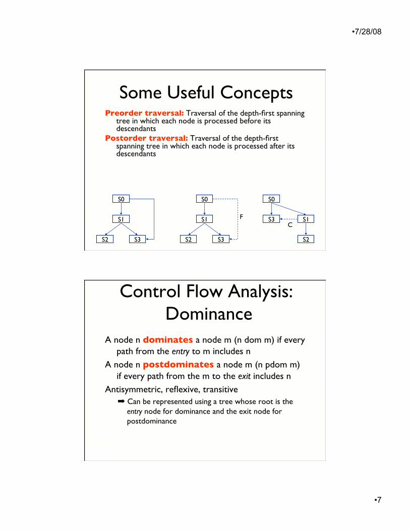
Some Useful Concepts Depth-First Search (DFS): Visits descendants before
visiting siblings Depth-first spanning tree: All nodes, only edges
traversed in the DFS Depth-first presentation: spanning tree + remaining
edges (marked) • Forward edges: node ➡ direct descendant • Back edges: node ➡ ancestor in the tree • Cross edges: node ➡ neither ancestor nor descendant
S1
S3
S0
S2
S1
S3
S0
S2
F S3 S1
S0
S2
C
• 7/28/08
• 7
Some Useful Concepts Preorder traversal: Traversal of the depth-first spanning
tree in which each node is processed before its descendants
Postorder traversal: Traversal of the depth-first spanning tree in which each node is processed after its descendants
S1
S3
S0
S2
S1
S3
S0
S2
F S3 S1
S0
S2
C
Control Flow Analysis: Dominance
A node n dominates a node m (n dom m) if every path from the entry to m includes n
A node n postdominates a node m (n pdom m) if every path from the m to the exit includes n
Antisymmetric, reflexive, transitive ➡ Can be represented using a tree whose root is the
entry node for dominance and the exit node for postdominance

• 7/28/08
• 8
Control Flow Analysis: Dominance
S1
S3
S4
S5
entry
exit
T
S2
S6
F
CFG Dominance Tree
S1
S3
S4
S5
entry
S2
S6
exit
T F
Control Flow Analysis: Dominance
S1
exit
entry
S2 S5
S6
S4
S3
S1
S3
S4
S5
entry
exit
T
S2
S6
F
CFG
T F
Postdominance Tree
• 7/28/08
• 9
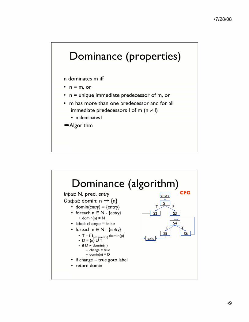
Dominance (properties)
n dominates m iff
• n = m, or • n = unique immediate predecessor of m, or • m has more than one predecessor and for all
immediate predecessors l of m (n ≠ l) • n dominates l
➡Algorithm
Dominance (algorithm) Input: N, pred, entry Output: domin: n → {n}
• domin(entry) = {entry} • foreach n ∈ N - {entry}
• domin(n) = N • label: change = false • foreach n ∈ N - {entry}
• T = ∩p ∈ pred(n) domin(p) • D = {n} ∪ T • if D ≠ domin(n)
– change = true – domin(n) = D
• if change = true goto label • return domin
S1
S3
S4
S5
entry
exit
T
S2
S6 F
CFG
T F
• 7/28/08
• 10
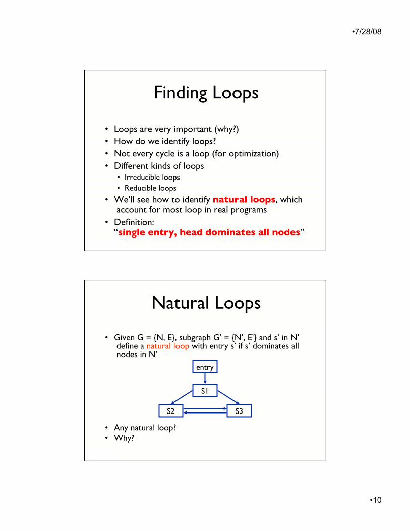
Finding Loops
• Loops are very important (why?) • How do we identify loops? • Not every cycle is a loop (for optimization) • Different kinds of loops
• Irreducible loops • Reducible loops
• We’ll see how to identify natural loops, which account for most loop in real programs
• Definition:�“single entry, head dominates all nodes”
Natural Loops
• Given G = {N, E}, subgraph G’ = {N’, E’} and s’ in N’ define a natural loop with entry s’ if s’ dominates all nodes in N’
• Any natural loop? • Why?
S2
S1
S3
entry

• 7/28/08
• 11
Using Dominance to Find Loops
S1
S3
S4
S5
entry
exit
T
S2
S6 F
CFG Dominance
Tree S1
S3
S4
S5
entry
S2
S6
exit T F
Dominance trees can be used to identify loops Back edge = t → h, h dominates t
Natural loop = given a back edge t → h, its natural loop is the subgraph consisting of: • node h (loop header) • all nodes dominated by h that can reach t w/o traversing h • all edges that connect nodes in this set
Example S1
S2
S3
S4
S5 S6
S7
S8
S9 S10
Find back edges and associated loops

• 7/28/08
• 12
Applications of Control Flow
Further analyses • Data-flow, reachability, …
Program understanding • Program structure and flow are made explicit
Software complexity • From the structural standpoint
Structural coverage in testing • Statement, branch, path, …
Program Analysis
Data-Flow Analysis
• 7/28/08
• 13
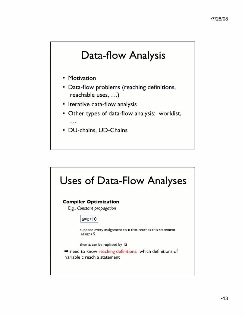
Data-flow Analysis
• Motivation • Data-flow problems (reaching definitions,
reachable uses, …)
• Iterative data-flow analysis • Other types of data-flow analysis: worklist,
… • DU-chains, UD-Chains
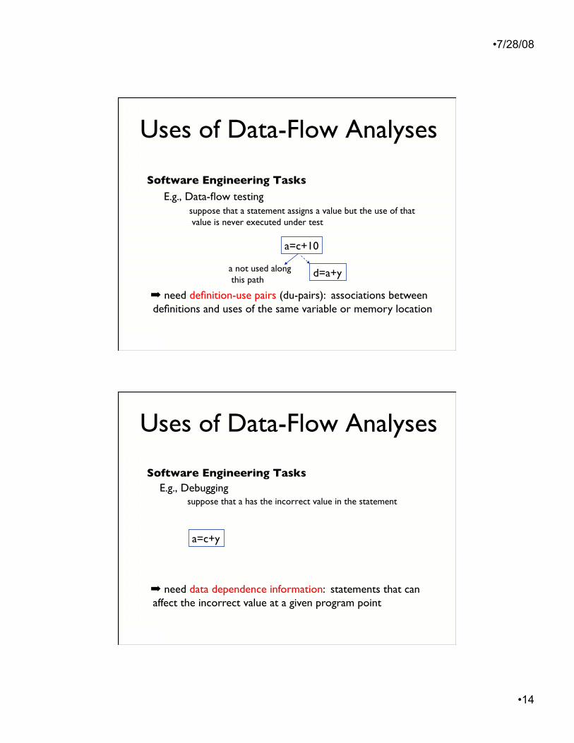
Uses of Data-Flow Analyses
Compiler Optimization E.g., Constant propagation
suppose every assignment to c that reaches this statement assigns 5
then a can be replaced by 15
a=c+10
➡ need to know reaching definitions: which definitions of variable c reach a statement
• 7/28/08
• 14
Software Engineering Tasks E.g., Data-flow testing
suppose that a statement assigns a value but the use of that value is never executed under test
a=c+10
d=a+y a not used along this path
Uses of Data-Flow Analyses
➡ need definition-use pairs (du-pairs): associations between definitions and uses of the same variable or memory location
Uses of Data-Flow Analyses
Software Engineering Tasks E.g., Debugging
suppose that a has the incorrect value in the statement
a=c+y
➡ need data dependence information: statements that can affect the incorrect value at a given program point
• 7/28/08
• 15
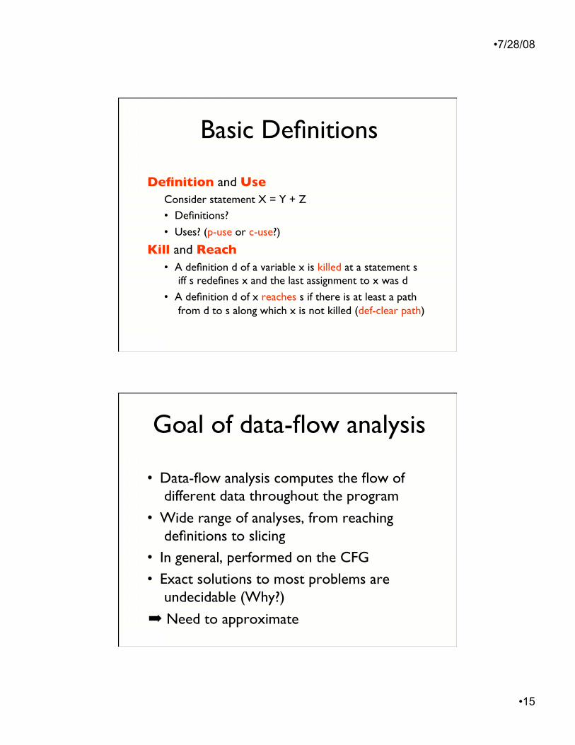
Basic Definitions
Definition and Use Consider statement X = Y + Z • Definitions?
• Uses? (p-use or c-use?) Kill and Reach
• A definition d of a variable x is killed at a statement s iff s redefines x and the last assignment to x was d
• A definition d of x reaches s if there is at least a path from d to s along which x is not killed (def-clear path)
Goal of data-flow analysis
• Data-flow analysis computes the flow of different data throughout the program
• Wide range of analyses, from reaching definitions to slicing
• In general, performed on the CFG • Exact solutions to most problems are
undecidable (Why?)
➡ Need to approximate

• 7/28/08
• 16
Safety and Precision
• Can you define safety and precision? • Are they related? • Can you give some examples?
• Is imprecision a problem only for data-flow analysis?
Safety and Precision
Approximate analysis can overestimate the solution: • Solution contains all actual information plus some spurious
information • This type of analysis is safe or conservative
Approximate analysis can underestimate the solution: • Solution may not contain all actual information • This type of analysis in unsafe
For optimization, need conservative, safe analysis For software engineering tasks, may be able to use unsafe
analysis information Major challenge for data-flow analysis: provide safe yet
precise (i.e., minimize the spurious information) information in an efficient way

• 7/28/08
• 17
Compute the flow of data to points in the program — e.g., • Where does the assignment to I
in statement 1 reach? • Where does the expression
computed in statement 2 reach? • Which uses of variable J are
reachable from the end of B1? Points in a basic block:
• before first statement • after last statement • between statements
1. I := 2 2. J := I + 1
3. I := 1
4. J := J + 1
5. J := J - 4
B1
B2
B3
B4
Data-Flow Problems
Reaching Definitions
Where are the definitions in the program? • Of variable I: • Of variable J:
Which basic blocks (before block) do these definitions reach? • Def 1 reaches • Def 2 reaches • Def 3 reaches • Def 4 reaches • Def 5 reaches
Problem:
Determine the set of definitions that reach a point in the program
1. I := 2 2. J := I + 1
3. I := 1
4. J := J + 1
5. J := J - 4
B1
B2
B3
B4

• 7/28/08
• 18
Reaching Definitions
Where are the definitions in the program? • Of variable I: 1, 3 • Of variable J: 2, 4, 5
Which basic blocks (before block) do these definitions reach? • Def 1 reaches B2 • Def 2 reaches B1, B2, B3 • Def 3 reaches B1, B3, B4 • Def 4 reaches B4 • Def 5 reaches exit
Typically solved by creating a set of data-flow equations
1. I := 2 2. J := I + 1
3. I := 1
4. J := J + 1
5. J := J - 4
B1
B2
B3
B4
Problem:
Determine the set of definitions that reach a point in the program
Iterative Reaching Definitions
Iterative Method: 1. Compute two kinds of local information
(i.e., within a basic block) GEN[B] is the set of definitions that are created
(generated) within B KILL[B] is the set of definitions in the program
that are killed if they reach B’s entry
2. Compute two other sets by propagation IN[B] is the set of definitions that reach the
beginning of B OUT[B] is the set of definitions that reach the
end of B
1. I := 2 2. J := I + 1
3. I := 1
4. J := J + 1
5. J := J - 4
B1
B2
B3
B4

• 7/28/08
• 19
1. I := 2 2. J := I + 1
3. I := 1
4. J := J + 1
5. J := J - 4
B1
B2
B3
B4
Iterative Method (cont’d):
Propagation method:
• Initialize IN[B], OUT[B] sets for all B • Iterate over all B until there are no
changes in IN[B] and OUT[B], computed as • IN[B] = ∪ OUT[P], P is a pred. of B • OUT[B] = GEN[B] ∪ (IN[B] – KILL[B])
Iterative Reaching Definitions
OUT[B]
IN[B]
GEN[B] KILL[B]
B
algorithm ReachingDefinitions Input: CFG w/ GEN[B], KILL[B] for all B Output: IN[B], OUT[B] for all B begin ReachingDefinitions
IN[B]=empty; OUT[B]=GEN[B], for all B; change = true while change do begin
change = false foreach B do begin
In[B] = union OUT[P], P is a predecessor of B Oldout = OUT[B] OUT[B] = GEN[B] U (IN[B] – KILL[B]) if OUT[B] != Oldout then change = true
endfor endwhile
end Reaching Definitions
Iterative Reaching Definitions

• 7/28/08
• 20
Iterative Reaching Definitions
• Where is imprecision affecting the computation?
• Is the algorithm guaranteed to converge?�Why or why not?
• What is the worst-case time complexity? • What is the worst-case space complexity? • Which visiting order could improve worst
-case time complexity? By how much?
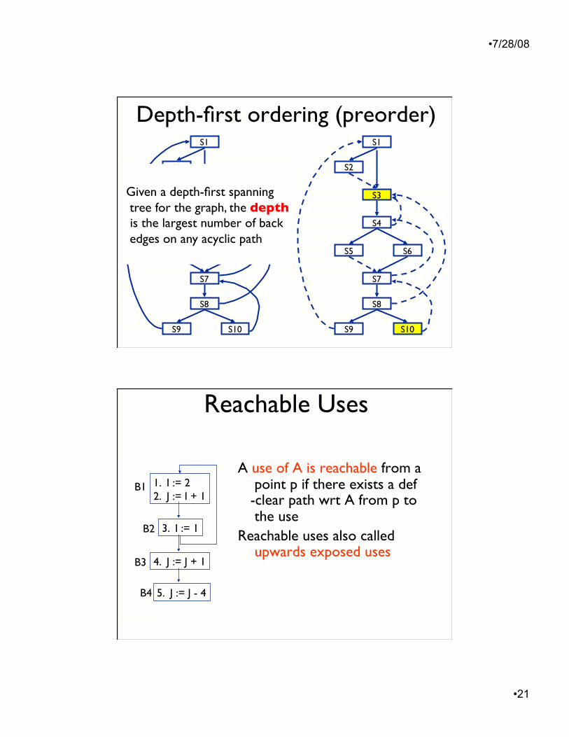
Depth-first ordering (preorder) S1
S2
S3
S4
S5 S6
S7
S8
S9 S10
S1
S2
S3
S4
S5 S6
S7
S8
S9 S10
• 7/28/08
• 21
Depth-first ordering (preorder) S1
S2
S3
S4
S5 S6
S7
S8
S9 S10
S1
S2
S3
S4
S5 S6
S7
S8
S9 S10
Given a depth-first spanning tree for the graph, the depth is the largest number of back edges on any acyclic path
A use of A is reachable from a point p if there exists a def-clear path wrt A from p to the use
Reachable uses also called upwards exposed uses
Reachable Uses
1. I := 2 2. J := I + 1
3. I := 1
4. J := J + 1
5. J := J - 4
B1
B2
B3
B4
• 7/28/08
• 22
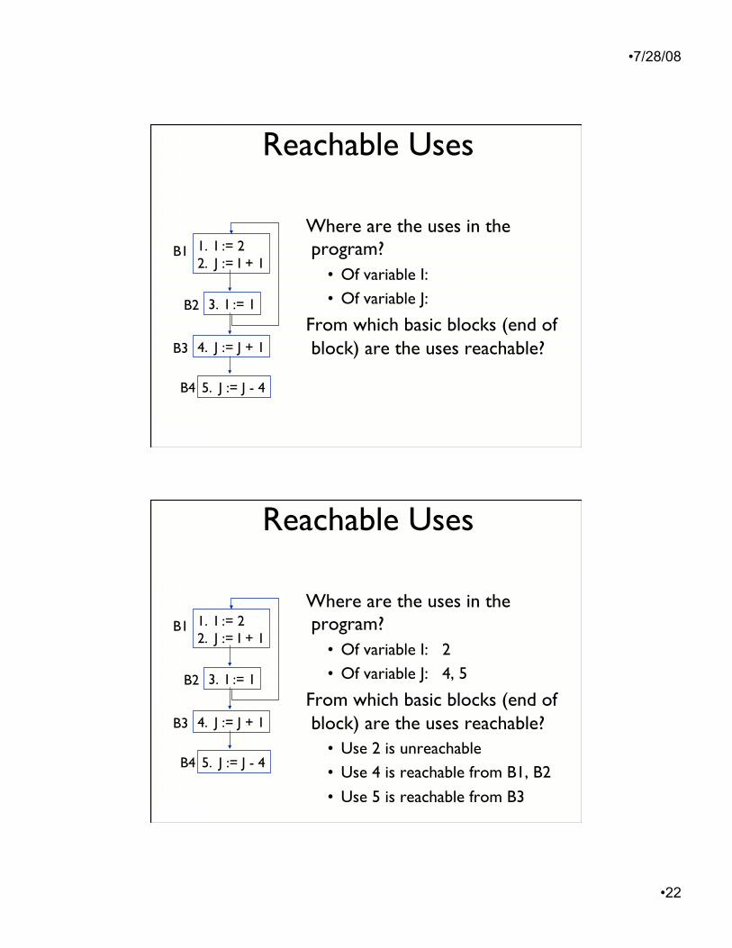
Where are the uses in the program?
• Of variable I: 2.1 • Of variable J: 4.2, 5.1
From which basic blocks (end of block) are the uses reachable?
Reachable Uses
1. I := 2 2. J := I + 1
3. I := 1
4. J := J + 1
5. J := J - 4
B1
B2
B3
B4
Where are the uses in the program?
• Of variable I: 2 • Of variable J: 4, 5
From which basic blocks (end of block) are the uses reachable?
• Use 2 is unreachable • Use 4 is reachable from B1, B2
• Use 5 is reachable from B3
Reachable Uses
1. I := 2 2. J := I + 1
3. I := 1
4. J := J + 1
5. J := J - 4
B1
B2
B3
B4
• 7/28/08
• 23
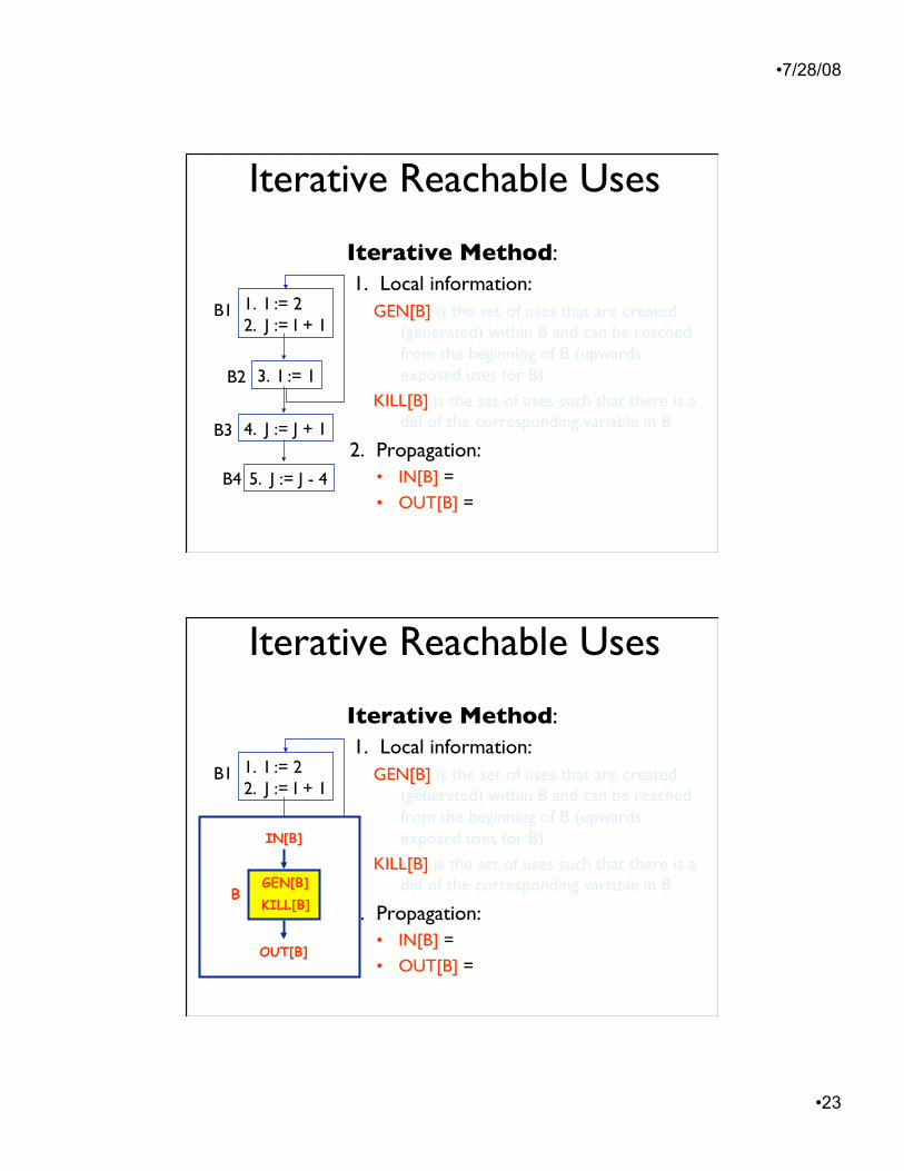
Iterative Reachable Uses
Iterative Method: 1. Local information:
GEN[B] is the set of uses that are created (generated) within B and can be reached from the beginning of B (upwards exposed uses for B)
KILL[B] is the set of uses such that there is a def of the corresponding variable in B
2. Propagation: • IN[B] =
• OUT[B] =
1. I := 2 2. J := I + 1
3. I := 1
4. J := J + 1
5. J := J - 4
B1
B2
B3
B4
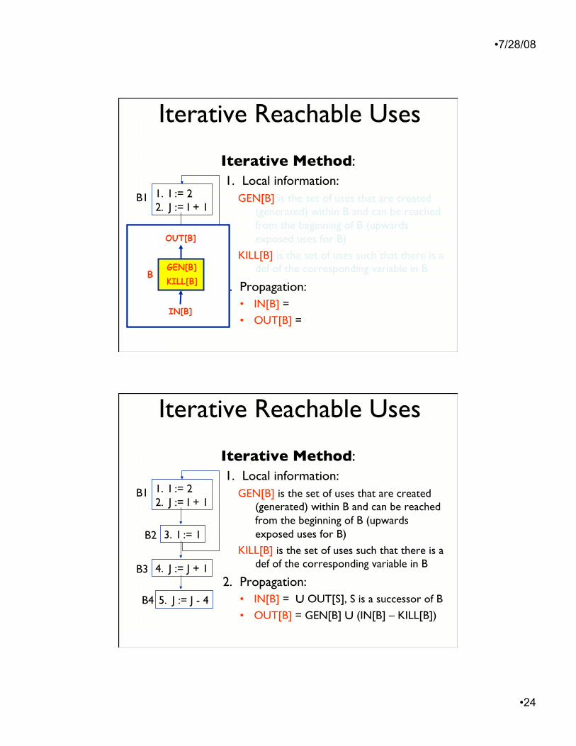
Iterative Reachable Uses
Iterative Method: 1. Local information:
GEN[B] is the set of uses that are created (generated) within B and can be reached from the beginning of B (upwards exposed uses for B)
KILL[B] is the set of uses such that there is a def of the corresponding variable in B
2. Propagation: • IN[B] =
• OUT[B] =
1. I := 2 2. J := I + 1
3. I := 1
4. J := J + 1
5. J := J - 4
B1
B2
B3
B4 OUT[B]
IN[B]
GEN[B] KILL[B]
B
• 7/28/08
• 24
Iterative Reachable Uses
Iterative Method: 1. Local information:
GEN[B] is the set of uses that are created (generated) within B and can be reached from the beginning of B (upwards exposed uses for B)
KILL[B] is the set of uses such that there is a def of the corresponding variable in B
2. Propagation: • IN[B] =
• OUT[B] =
1. I := 2 2. J := I + 1
3. I := 1
4. J := J + 1
5. J := J - 4
B1
B2
B3
B4 OUT[B]
IN[B]
GEN[B] KILL[B]
B
IN[B]
OUT[B]
GEN[B] KILL[B]
B
Iterative Reachable Uses
Iterative Method: 1. Local information:
GEN[B] is the set of uses that are created (generated) within B and can be reached from the beginning of B (upwards exposed uses for B)
KILL[B] is the set of uses such that there is a def of the corresponding variable in B
2. Propagation: • IN[B] = ∪ OUT[S], S is a successor of B
• OUT[B] = GEN[B] ∪ (IN[B] – KILL[B])
1. I := 2 2. J := I + 1
3. I := 1
4. J := J + 1
5. J := J - 4
B1
B2
B3
B4

• 7/28/08
• 25
algorithm ReachableUses Input: CFG w/ GEN[B], KILL[B] for all B Output: IN[B], OUT[B] for all B begin ReachableUses
OUT[B]=GEN[B], IN[B]=empty, for all B; change = true while change do begin
change = false foreach B do begin
IN[B] = union OUT[S], S is a successor of B OldOUT = OUT[B] OUT[B] = GEN[B] U (IN[B] – KILL[B]) If OUT[B] != OldOUT then change = true
endfor endwhile
end ReachableUses
Iterative Reachable Uses
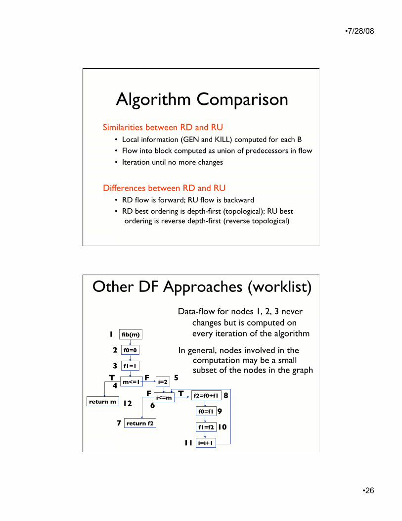
Similarities between RD and RU
Differences between RD and RU
Algorithm Comparison
• 7/28/08
• 26
Similarities between RD and RU • Local information (GEN and KILL) computed for each B • Flow into block computed as union of predecessors in flow
• Iteration until no more changes
Differences between RD and RU • RD flow is forward; RU flow is backward • RD best ordering is depth-first (topological); RU best
ordering is reverse depth-first (reverse topological)
Algorithm Comparison
Data-flow for nodes 1, 2, 3 never changes but is computed on every iteration of the algorithm 1
return f2
i=2
i<=m return m
fib(m)
f0=0
m<=1
f1=1
i=i+1
f1=f2
f0=f1
f2=f0+f1 T
T F
F
2
3
4 5
6 8
7 10
11
9 12
Other DF Approaches (worklist)
In general, nodes involved in the computation may be a small subset of the nodes in the graph
• 7/28/08
• 27
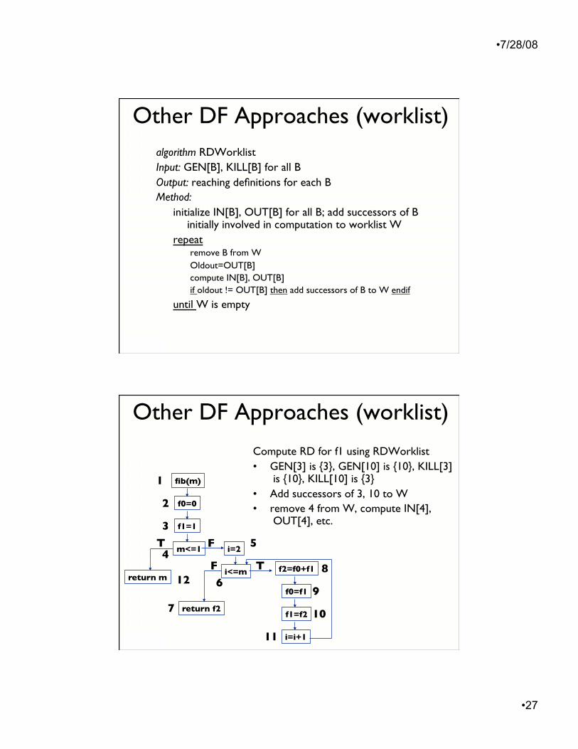
Other DF Approaches (worklist) algorithm RDWorklist Input: GEN[B], KILL[B] for all B Output: reaching definitions for each B Method:
initialize IN[B], OUT[B] for all B; add successors of B initially involved in computation to worklist W
repeat remove B from W Oldout=OUT[B] compute IN[B], OUT[B] if oldout != OUT[B] then add successors of B to W endif
until W is empty
Compute RD for f1 using RDWorklist • GEN[3] is {3}, GEN[10] is {10}, KILL[3]
is {10}, KILL[10] is {3} • Add successors of 3, 10 to W • remove 4 from W, compute IN[4],
OUT[4], etc.
Other DF Approaches (worklist)
1
return f2
i=2
i<=m return m
fib(m)
f0=0
m<=1
f1=1
i=i+1
f1=f2
f0=f1
f2=f0+f1 T
T F
F
2
3
4 5
6 8
7 10
11
9 12


![BIOMECHANICZNA ANALIZ WCHODZENIA A NA SCHODY ORAZ … (41).pdf · 2015. 7. 16. · Badani X PI P3 P4 P5 P6 P7 P8 bp bk bp bk bp bk bp bk bp bk bp bk bp bk Ls [mm] 420 1571 1172 453](https://img.pdfslide.net/doc/110x75/60aa279aa5b98926d7795c28/biomechaniczna-analiz-wchodzenia-a-na-schody-oraz-41pdf-2015-7-16-badani.jpg)


![Further study of Advanced MIMO receiverpeng/MIMO-Receiver.pdf · b k [b1 b2 bk 1 bk 1 bN],bk [b1 b2 bk 1 1 bk 1 bN] and bk [b1 b2 bk 1 1 bk 1 bN] Problem: the number of combinations](https://img.pdfslide.net/doc/110x75/5fe7675492953575f353f746/further-study-of-advanced-mimo-receiver-pengmimo-b-k-b1-b2-bk-1-bk-1-bnbk.jpg)