Progress in Oceanography - Massachusetts Institute of …ocean.mit.edu/~stephd/proweetal_progoce_2011.pdf · 2016-06-05 · Top-down control of marine phytoplankton diversity in a

Progress in Oceanography xxx (2011) xxx–xxx

Contents lists available at SciVerse ScienceDirect

Progress in Oceanography

journal homepage: www.elsevier .com/ locate /pocean

Top-down control of marine phytoplankton diversity in a global ecosystem model

A.E. Friederike Prowe a,⇑, Markus Pahlow a, Stephanie Dutkiewicz b, Michael Follows b, Andreas Oschlies a

a IFM–GEOMAR, Leibniz Institute of Marine Sciences at the University of Kiel, Düsternbrooker Weg 20, 24105 Kiel, Germanyb Department of Earth, Atmospheric, and Planetary Sciences, Massachusetts Institute of Technology, 77 Massachusetts Avenue, Cambridge, MA 02139, USA

a r t i c l e i n f o

Article history:Received 22 December 2010Received in revised form 22 November 2011Accepted 29 November 2011Available online xxxx

0079-6611/$ - see front matter � 2011 Elsevier Ltd. Adoi:10.1016/j.pocean.2011.11.016

⇑ Corresponding author. Tel.: +49 431 600 4032; faE-mail address: [email protected] (A.E.F. Pro

Please cite this article in press as: Prowe, A.E.F.,(2011), doi:10.1016/j.pocean.2011.11.016

a b s t r a c t

The potential of marine ecosystems to adapt to ongoing environmental change is largely unknown,making prediction of consequences for nutrient and carbon cycles particularly challenging. Realizing thatbiodiversity might influence the adaptation potential, recent model approaches have identified bottom-up controls on patterns of phytoplankton diversity regulated by nutrient availability and seasonality.Top-down control of biodiversity, however, has not been considered in depth in such models. Here wedemonstrate how zooplankton predation with prey-ratio based food preferences can enhancephytoplankton diversity in a ecosystem-circulation model with self-assembling community structure.Simulated diversity increases more than threefold under preferential grazing relative to standard den-sity-dependent predation, and yields better agreement with observed distributions of phytoplanktondiversity. The variable grazing pressure creates refuges for less competitive phytoplankton types, whichreduces exclusion and improves the representation of seasonal phytoplankton succession during blooms.The type of grazing parameterization also has a significant impact on primary and net community pro-duction. Our results demonstrate how a simple parameterization of a zooplankton community responseaffects simulated phytoplankton community structure, diversity and dynamics, and motivates develop-ment of more detailed representations of top-down processes essential for investigating the role of diver-sity in marine ecosystems.

� 2011 Elsevier Ltd. All rights reserved.

1. Introduction

Evidence is increasing that biodiversity influences productivityand stability of ecosystems across trophic levels in both marineand terrestrial realms (Worm et al., 2006; Ptacnik et al., 2008).Theoretical considerations indicate that higher species richnesscan increase ecosystem stability (Tilman et al., 1997; Yachi andLoreau, 1999). However, experimental observations demonstratingdiversity effects in marine pelagic ecosystems are scarce and therole of diversity for these ecosystems is not well known (Duffyand Stachowicz, 2006; Ptacnik et al., 2010). In light of anticipatedchanges in marine phytoplankton community structure (Moranet al., 2010; Boyd and Doney, 2002; Worm et al., 2002; Cardinaleet al., 2006) and its effects on ecosystem structure and functioning(Bopp et al., 2005; Manizza et al., 2010), what shapes marinephytoplankton diversity is becoming a central research question.

Diversity is linked to differences in traits, e.g. optimal tempera-ture for growth, within a community of species. One approach tocapturing diversity in models is to formulate trade-offs betweenthe different traits, which allows the system to emerge adaptivelyfrom environmental conditions (Norberg, 2004). This adaptivedynamics approach has been applied to models of local ecosystems

ll rights reserved.

x: +49 431 600 4469.we).

et al. Top-down control of mar

only (Bruggeman and Kooijman, 2007; Merico et al., 2009). On theglobal scale, prognostic models have made efforts to resolve someof the functional diversity of phytoplankton by increasing thenumber of plankton functional types (e.g. Le Quéré et al., 2005).With a stronger focus on traits, an alternative approach hasemployed an explicit community consisting of a large number ofphytoplankton types (Follows et al., 2007) differing randomly insize, optimal temperature, growth parameters, and sinking speed(Section 2.1).

Recent studies using the Follows et al. (2007) model havedemonstrated how distinct phytoplankton communities emerge ina global ocean model through bottom-up control by resourceavailability, where the emergent communities differed in their com-petitiveness for resources in different environments (Dutkiewiczet al., 2009; Barton et al., 2010). Besides bottom-up control, how-ever, top-down mechanisms by consumers (predators) can shapediversity and ecosystem structure (Chesson, 2000; Worm et al.,2002; Chase et al., 2002). In models, structure and functioning ofthe simulated ecosystem are very sensitive to the choice of preda-tion formulation (Anderson et al., 2010). In the previous studiesbased on the Follows et al. (2007) self-assembling ecosystem model,zooplankton predation was modeled in a simplistic way using twozooplankton types with similar Holling type II grazing responsesand fixed preferences for each phytoplankton type. Here we showhow a more flexible representation of the predation process can help

ine phytoplankton diversity in a global ecosystem model. Prog. Oceanogr.

http://dx.doi.org/10.1016/j.pocean.2011.11.016

mailto:[email protected]


http://www.sciencedirect.com/science/journal/00796611

http://www.elsevier.com/locate/pocean


2 A.E.F. Prowe et al. / Progress in Oceanography xxx (2011) xxx–xxx

to better understand the emergence of phytoplankton diversity viatop-down controls in a global ecosystem-circulation model.

2. Methods

2.1. The ecosystem model

The model used in this study is the Massachusetts Institute ofTechnology general circulation model (MITgcm) with the ‘‘Darwin’’ecosystem module (Follows et al., 2007). The latter comprisesprognostic equations of state for four nutrients (phosphorus,nitrogen, iron and silica), 78 phytoplankton types, one large andone small zooplankton type, dissolved and particulate organicmatter. Phosphorus is used as the main currency of the model.Temperature-dependent phytoplankton growth takes into accountlimitation by light, including effects of self shading, and by aLiebig-type limitation by the most limiting nutrient according toa Michaelis–Menten formulation. Phytoplankton losses include alinear mortality, sinking and zooplankton predation, which is for-mulated as a Holling type II functional response. Both zooplanktontypes have the same maximum grazing rate and half-saturationconcentration for grazing. Their grazing rates differ only in thepreferences for the different phytoplankton types, which are as-signed according to size and palatability. The export of organicmatter to depth occurs mainly via particulate organic matter pro-duced by phytoplankton mortality, sloppy feeding and zooplanktonegestion and mortality. Sinking of phytoplankton plays a minorrole. At the start of the simulation, the model ocean is seeded withthe different phytoplankton types each characterized by a set ofrandomly assigned trait parameters. Phytoplankton types differin cell size (small or large), nutrient requirements, half-saturationconcentrations for nutrient uptake, light-limited growth, optimaltemperature, and sinking speed (see Dutkiewicz et al. (2009) forequations and a detailed list of phytoplankton parameter ranges).The standard model setup in this study is identical to the one usedby Dutkiewicz et al. (2009, Table A.1) except for a reduced zoo-plankton mortality (from mZ = 0.033 d�1 to mZ = 0.013 d�1), whichdoes not result in qualitative differences in diversity compared tothe preceding studies. Three additional configurations employmodified predation formulations (see Sections 2.2 and 3.1, andTable 1). For each model configuration an ensemble of fiveintegrations with different random phytoplankton parameter setsare performed. Here, we are using five of the random parametersets also used by Dutkiewicz et al. (2009) for better comparability.

Table 1Model configurations. Parameter values of maximum grazing rate (gmax) and half-saturatiodiversity as Shannon Index and as number of phytoplankton types exceeding threshold coaverage total phytoplankton biomass (0–55 m), primary production (PP) and net commun

Configuration LGNS low grazing andno switching

Switching NojP

kmmol P m�3 0.1

gmax d�1 0.5

Ave. diversity No. types 6.5Ave. diversity (Pth � 10) No. types 5.8Ave. diversity (Pth/10) No. types 7.0Max. diversity No. types 15.9Max. diversity (Pth � 10) No. types 14.3Max. diversity (Pth/10) No. types 16.9Ave. Shannon Index 0.7Max. Shannon Index 1.5Ave. total phytoplankton 10�3 mmol P m�3 8.4Ave. PP g C m�2 d�1 0.18Ave. NCP g C m�2 d�1 0.09

Please cite this article in press as: Prowe, A.E.F., et al. Top-down control of ma(2011), doi:10.1016/j.pocean.2011.11.016

The physical model is forced offline by the ECCO-GODAE stateestimates (Wunsch and Heimbach, 2007). The coupled ecosys-tem-circulation model is integrated on a global grid of 1� resolu-tion with 24 depth levels for 10 years, by which time it mostlydisplays a repeating annual cycle in nutrients and primary produc-tion. Results are presented as the average of the ensemble of fiveintegrations (see Appendix B, Fig. B.1), averaged over 0–55 m depthin the 10th year (unless noted otherwise).

2.2. High/low grazing configuration

The Holling type II predation formulation describes the grazingprocess in terms of two compound parameters, namely the maxi-mum grazing rate (gmax) and the half-saturation concentration forgrazing jP

k

� �, which by themselves cannot be directly interpreted

in mechanistic terms. In this study, we investigate the sensitivityof the model results to changes in the grazing formulation by usingtwo parameterizations characterized by high and low grazing rates(the high grazing and low grazing setups, respectively). For the highgrazing setup, we derive gmax and jP

k from a size-based mechanisticfeeding-strategy model describing encounter and capture betweena suspension feeder and its immotile phytoplankton prey (seeAppendix A for a detailed description). In the simplest configura-tion this mechanistic model reduces to a type II formulation thatis structurally identical to the type II formulation used previously(Dutkiewicz et al., 2009; Barton et al., 2010). However, this ap-proach allows us to determine gmax and jP

k from biologically mean-ingful parameters describing the grazing process. The mechanisticmodel results in notably higher gmax and lower jP

k than the originalparameterization, and is thus referred to as high grazing setup incontrast to the low grazing standard configuration.

2.3. Diversity measures

We define the metric ‘‘diversity’’ to be the number of phyto-plankton types that exceed a low threshold biomass concentrationof Pth = 10�8 mmol m�3 (in units of phosphorus; following Bartonet al., 2010). Since phytoplankton types in the model are distin-guished by functional traits such as maximum growth rates, themodeled functional diversity does not necessarily compare quanti-tatively to observational measures of (taxonomic) species richness.The modeled diversity depends to a limited extent on the numberof phytoplankton types initialized (as indicated by related simula-tions with different numbers of phytoplankton types; Prowe et al.,2012) as well as on the chosen threshold concentration. Therefore

n concentration for grazing jPk

� �. Global annual average and maximum phytoplankton

ncentration Pth for Pth = 10�8 mmol P m�3 (default), Pth � 10 and Pth/10. Global annuality production (NCP; both 0–100 m).

LGAS low grazing andactive switching

HGNS high grazing andno switching

HGAS high grazing andactive switching

Active No Active0.1 0.027 0.027

0.5 1.0 1.0

10.5 4.6 21.39.4 4.1 19.111.3 5.0 23.037.4 10.4 55.335.0 9.1 52.238.8 11.1 59.41.1 0.6 2.02.6 1.3 3.311.5 1.92 5.70.21 0.09 0.160.11 0.04 0.09

rine phytoplankton diversity in a global ecosystem model. Prog. Oceanogr.


A.E.F. Prowe et al. / Progress in Oceanography xxx (2011) xxx–xxx 3

we also calculated the Shannon Index (H) from the biomass con-centrations (P) of all phytoplankton types

H ¼ �Xn

j

pjlnðpjÞ ; pj ¼PjP

rPr: ð1Þ

Though not intuitively related to ecological diversity, H considersthe joint influence of species richness and evenness (Stirling andWilsey, 2001) and takes into account all phytoplankton types with-out the need of a threshold concentration.

3. Grazing parameterizations

3.1. ‘‘No switching’’ and ‘‘active switching’’ configurations

In the standard configuration of the model (Dutkiewicz et al.,2009), the Holling type II formulation describes ingestion (Ijk) ofphytoplankton type j by zooplankton type k depending on the bio-mass concentration of phytoplankton type j (Pj)

Ijk ¼ gmax

qjkPj

jPk þ

Pr

qrkPr: ð2Þ

Each of the two zooplankton types k is assigned different, but fixedpreferences (qjk) for each phytoplankton type j which are set to val-ues between 0 and 1 according to the body sizes of both zooplank-ton and phytoplankton as well as the phytoplankton functional type(e.g. diatoms, prochlorococcus analogues).

This setup relies on the assumption that the impact of the entiregrazer community can be represented by two functional types withfixed food preferences. An explicit representation of the predatorcommunity response would require adding a large number of statevariables. Instead, we here parameterize the grazer communityresponse implicitly by assuming that consumers covary with theresources on which they are specialized. Such a communityresponse can be captured by replacing the fixed food preferences(q) by selectivities (r), which are calculated from q and scaledby the biomass of each phytoplankton type j (Fasham et al.,1990) relative to total phytoplankton biomass available for grazing

rj ¼qjPjP

rqrPr

: ð3Þ

When a food type declines, the corresponding selectivity, and henceingestion, decreases, while an increasing food type will be selectedmore strongly and thus suffer from more intense predation.

This grazing formulation is referred to as active switching(Gentleman et al., 2003), while constant food preferences implyno switching. Switching is an effective means for promotingcoexistence (Hutson, 1984) and stability in simulated ecosystems(Murdoch and Oaten, 1975) and has been implemented in severalecosystem models (Fasham et al., 1990; Fasham et al., 1993;Aumont et al., 2003; Aumont and Bopp, 2006). At the same time,this formulation can cause total ingestion to decrease although to-tal available food increases, which was thought to be unbiologicalbehavior (Gentleman et al., 2003). A recent modeling approachdemonstrates, however, how reduced ingestion rates at higherprey concentrations can arise from copepods switching feedingstrategies in the face of predation risk (Mariani and Visser, 2010).Active switching between similar kinds of prey was observed inmicrozooplankton (see Strom et al., 2000) and copepods (Paffenhö-fer, 1984). Copepods also actively switch between kinds of prey byshifting to different feeding strategies (Jonsson and Tiselius, 1990;Saiz and Kiørboe, 1995; Kiørboe et al., 1996). Here we interpret ac-tive switching not only as behavioral change of one predator type,but as a compound effect of the unresolved predator community.

Please cite this article in press as: Prowe, A.E.F., et al. Top-down control of mar(2011), doi:10.1016/j.pocean.2011.11.016

3.2. Grazing pressure

The choice of the grazing formulation is known to determinethe simulated dynamics of simple nutrient–phytoplankton–zoo-plankton (NPZ) systems. Density dependent phytoplankton growthor loss terms, which depend on the phytoplankton concentrationwith an exponent >1, as introduced by the active switching formu-lation, can promote coexistence of several phytoplankton types(Gross et al., 2009). Density independent formulations (expo-nent = 1), for example for the no switching formulation in ourmodel, lead to competitive exclusion. For grazing formulations thiscriterion for coexistence mathematically implies a positive slope ofthe clearance rate, I/P, as a function of P. This measure can also beused to characterize the effect of grazing formulations on the sta-bility of simple NPZ systems with one phytoplankton (Gentlemanand Neuheimer, 2008). Here we employ this measure to betterunderstand the effect of switching behavior on phytoplanktondiversity in a multi-phytoplankton type system. Instead of theterm ‘‘clearance rate’’, which refers to the volume of water whichzooplankton would entirely clear of prey given a certain ingestionrate, we use the term ‘‘specific grazing pressure’’ for the samequantity to stress the effect of grazing on the phytoplankton.

The specific grazing pressure (Gjk = Ijk/Pj) of zooplankton k foreach phytoplankton type j provides a measure of the strength ofpredation aside from effects of predator concentration. If prefer-ences (qjk) are constant, i.e. for no switching (Eq. (2)), it is given by

Gjk ¼Ijk

Pj¼ gmax

qjk

jPk þ

PrqrkPr

: ð4Þ

For selectivities changing with phytoplankton concentration (Eq.(3)), i.e. for active switching, it is

Gjk ¼ gmax

qjkPj

jPk

PrqrkPr þ

PrqrkP2

r

: ð5Þ

The slope of Gjk is calculated as the first derivative with respect tothe phytoplankton concentration of type j (@ Gjk/@Pj). For no switch-ing, @Gjk/@ Pj is negative for all Pj

@Gjk

@Pj¼ �gmax

q2jk

jPk þ

PrqrkPr

� �2 < 0 ð6Þ

For active switching, @Gjk/@Pj is given by

@Gjk

@Pj¼ gmax

qjk

Pr–jqrkP2

r � qjkP2j þ jP

k

Pr–jqrkPr

� �P

rqrkP2r þ jP

k

PrqrkPr

� �2 ð7Þ

and can be positive or negative depending on qrk and Pj.The initial slope at Pj = 0 can be calculated from

@

@Pj

Ijk

Pj

� ��Pj¼0

¼ gmax

qjk

Pr–jqrkP2

r þ jPk

Pr–jqrkPr

� �P

rqrkP2r þ jP

k

PrqrkPr

� �2 ð8Þ

¼Pj¼0

gmax

qjkPrqrkP2

r þ jPk

PrqrkPr

> 0 ð9Þ

and is always positive. This indicates that Gjk increases up to a crit-ical phytoplankton concentration Pcrit

j which can be determined by

@Gjk

@Pj¼ 0() Pcrit

j ¼

ffiffiffiffiffiffiffiffiffiffiffiffiffiffiffiffiffiffiffiffiffiffiffiffiffiffiffiffiffiffiffiffiffiffiffiffiffiffiffiffiffiffiffiffiffiffiffiffiffiffiffiffiffiffiffiffiffiffiffiffiffiffiffiffi1qjk

Xr–j

qrkP2r þ jP

k

Xr–j

qrkPr

!vuut : ð10Þ

For a sigmoidal type III grazing functional response, as used forinstance by Yool et al. (2011), a similar result is obtained.

Active switching and no switching thus imply qualitativelydifferent behavior when phytoplankton concentrations change.




Active switching can promote coexistence by damping changes inindividual phytoplankton concentration as long as phytoplanktonconcentrations do not exceed Pcrit

j . No switching may promotedominance of individual phytoplankton types because it amplifieschanges in phytoplankton concentration. In the context of stabilityof NPZ models, a positive slope reduces oscillations and createsrefuges from predation for the phytoplankton (Gentleman andNeuheimer, 2008). A negative slope causes a positive feed-backbetween phytoplankton concentration and growth and destabi-lizes the system. Below, we show that the slope of the grazingpressure can also explain how active switching helps to generateniches for less abundant phytoplankton types and thereby enhancephytoplankton diversity. We compare results of the active and theno-switching formulations (Section 3.1), each with low and highgrazing rates from the original configuration and the mechanisticgrazing model (Section 2.2), respectively, yielding four configura-tions: low grazing and no switching (LGNS), low grazing and activeswitching (LGAS), high grazing and no switching (HGNS), and highgrazing and active switching (HGAS; Table 1).

4. Results and discussion

4.1. Phytoplankton diversity patterns

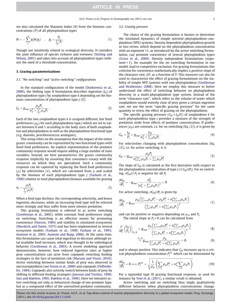
For LGNS (essentially the same as Barton et al. (2010)), phyto-plankton diversity, measured as the number of types exceedingPth = 10�8 mmol P m�3, averages 6.5 in the upper 55 m of the watercolumn (Fig. 1a). Diversity increases by 62% to an average of 10.5 inLGAS (Fig. 1b). For HGAS, diversity rises more than threefold to anaverage of 21.3 (Fig. 1d). Simply increasing grazing rates, however,does not necessarily increase diversity as can be seen in HGNS for

a

c

Fig. 1. Phytoplankton diversity. Annual average number of phytoplankton types exceedinfor abbreviations. The dots and circle in (a) mark the Atlantic Meridional Transect (AMT


which diversity decreases compared to LGNS to an average of 4.6species present (Fig. 1c).

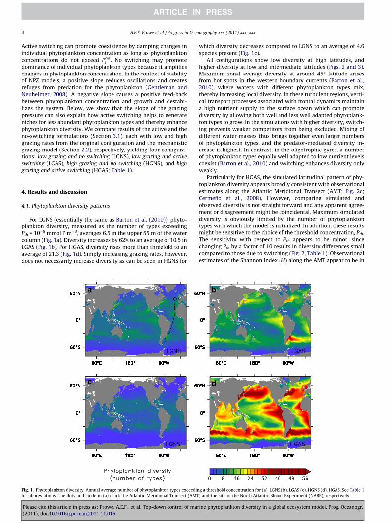
All configurations show low diversity at high latitudes, andhigher diversity at low and intermediate latitudes (Figs. 2 and 3).Maximum zonal average diversity at around 45� latitude arisesfrom hot spots in the western boundary currents (Barton et al.,2010), where waters with different phytoplankton types mix,thereby increasing local diversity. In these turbulent regions, verti-cal transport processes associated with frontal dynamics maintaina high nutrient supply to the surface ocean which can promotediversity by allowing both well and less well adapted phytoplank-ton types to grow. In the simulations with higher diversity, switch-ing prevents weaker competitors from being excluded. Mixing ofdifferent water masses thus brings together even larger numbersof phytoplankton types, and the predator-mediated diversity in-crease is highest. In contrast, in the oligotrophic gyres, a numberof phytoplankton types equally well adapted to low nutrient levelscoexist (Barton et al., 2010) and switching enhances diversity onlyweakly.

Particularly for HGAS, the simulated latitudinal pattern of phy-toplankton diversity appears broadly consistent with observationalestimates along the Atlantic Meridional Transect (AMT; Fig. 2c;Cermeño et al., 2008). However, comparing simulated andobserved diversity is not straight forward and any apparent agree-ment or disagreement might be coincidental. Maximum simulateddiversity is obviously limited by the number of phytoplanktontypes with which the model is initialized. In addition, these resultsmight be sensitive to the choice of the threshold concentration, Pth.The sensitivity with respect to Pth appears to be minor, sincechanging Pth by a factor of 10 results in diversity differences smallcompared to those due to switching (Fig. 2, Table 1). Observationalestimates of the Shannon Index (H) along the AMT appear to be in

b

d

g a threshold concentration for (a), LGNS (b), LGAS (c), HGNS (d), HGAS. See Table 1) and the site of the North Atlantic Bloom Experiment (NABE), respectively.



a b

c d

Fig. 3. Phytoplankton diversity. Annual average Shannon Index for (a), LGNS (b), LGAS (c), HGNS (d), HGAS. See Table 1 for abbreviations.

a b

c d

Fig. 2. Latitudinal diversity gradient. Simulated surface layer diversity as (a, c), number of phytoplankton types and (b, d) Shannon Index. Diversity is shown in (a, b) as zonalaverage and in (c, d) along the Atlantic Meridional Transect (AMT). Observed taxonomic diversity shown in (c, d) as number of species (surface data) and as Shannon Index(right y-axes) is calculated from biomass of diatoms, dinoflagellates and coccolithophores along the AMT (circles; Cermeño et al., 2008). Model estimates of functionaldiversity do not necessarily compare quantitatively to observational estimates of taxonomic diversity. Observational estimates of the Shannon Index may include data fromthe surface as well as from greater depths (P. Cermeño, personal communication). The uncertainty bands in (a) and (c) denote the diversity range between the ensembleaverages of simulations with increased and decreased threshold concentration Pth compared to the standard configuration (Pth � 10 and Pth/10, respectively).


general higher than the simulations (Fig. 2d). No latitudinalgradient in H can be inferred from the observations along theAMT, possibly because these values include observations at differ-ent depths (Cermeño et al., 2008). In addition, both observational


diversity measures might be biased particularly at low latitudessince picophytoplankton were neglected (Aiken et al., 2009). Thisbias is, however, difficult to assess due to the unclear notion of‘‘species’’ for this group.



0 0.002 0.004 0.006 0.008 0.010

0.2

0.4

0.6

0.8

1

P1 concentration (mmol P m−3)

Pref

eren

ce o

r sel

ectiv

ity a ρ1 ρ2 σ1 σ2

0 0.002 0.004 0.006 0.008 0.010

10

20

30

Spec

ific

graz

ing

pres

sure

Gi

(m3 m

mol

P−1

d−1

)

P1 HGNS P2 HGNS P1 HGAS P2 HGAS

0 0.002 0.004 0.006 0.008 0.010

10

20

30

P1 concentration (mmol P m−3)

b

P1 LGNS P2 LGNS P1 LGAS P2 LGAS

Fig. 4. Idealized two-phytoplankton system with equal preferences. (a) Preference(q) for no switching (dashed lines) or selectivity (r) for active switching (solid lines).Phytoplankton P1 increases from 0 to 0.01 mmol P m�3, phytoplankton P2 remainsat 0.001 mmol P m�3. (b) Corresponding specific grazing pressure for high grazingand low grazing (see Table 1 for parameter values).


4.2. Mechanisms of diversity increase

The mechanism by which active switching promotes phyto-plankton diversity is illustrated by a simplified example with twoequally preferred (q1 = q2) phytoplankton types. When the concen-tration of type 1 (P1) increases from 0 to 0.01 mmol P m�3 with the

a b

d e

Fig. 5. Total phytoplankton biomass. (a) Annual average total phytoplankton biomass (0difference to LGNS. Zonal averages of total phytoplankton biomass are shown in (c) as a


concentration of type 2 (P2) fixed at 0.001 mmol P m�3, selectivityfor type 1 (r1) increases with increasing P1, while r2 decreases (Eq.(3), Fig. 4a). Increasing P1 leads to higher specific grazing pressure(G1) for small concentrations of P1 as r1 increases, but reduces G2

for the less abundant type P2 by increasing total phytoplanktonavailable for grazing (

Pr ½rrPr �; Fig. 4b). In this example, when

P1 > Pcrit1 ð¼ 0:006 mmol P m�3Þ any further increase of

Pr½rrPr �

leads to a reduction of G for both types. In contrast, under noswitching, G for both types always decreases with increasingconcentration of P1 (Eq. (6)).

By increasing the specific grazing pressure on the mostabundant phytoplankton types, active switching makes the lessabundant types more competitive. The initial slope of G (@Gjk/oPj)determines whether zooplankton predation can increase diversityin this way. For no switching, @Gjk/@Pj is always negative (Eq. (6))and therefore rewards growth of competitive types with reducedgrazing pressure, thereby increasing competitiveness and promot-ing dominance of already successful types. In contrast, the activeswitching formulation has a positive initial slope at Pj = 0 (Eq.(9)) and Gjk thus increases if concentrations of type j increase upto a critical concentration (see Section 3.2), so that growth of thistype is damped.

The strength of this increase in competitiveness is related to theinitial slope of G and depends on the values of gmax and jP

k . Forsmall gmax or large jP

k (compared toP

r ½rrPr �; LGAS) the initialslope is small (Fig. 4b) and the predator-mediated diversity in-crease is weaker than for HGAS (Fig. 1b and d). In contrast, noswitching favors the most resource-competitive type by reducingspecific grazing pressure with increasing concentration for all phy-toplankton types and across all concentrations. In a model ecosys-tem with one phytoplankton, this reduction in grazing pressurewith increasing phytoplankton biomass was shown to cause oscil-lations and thus reduces the stability of the system (Gentlemanand Neuheimer, 2008). The same property of the grazing functiontends to favor coexistence when applied to competing phytoplank-ton types. The variable grazing pressure creates additional limitingfactors for each phytoplankton type individually and thereby en-hances the number of competing phytoplankton types that cancoexist (Levin, 1970; Chase et al., 2002). Switching thus constitutes

c

f

–55 m depth) for LGNS is compared to (b) LGAS, (d) HGNS, and (e) HGAS as relativebsolute values and in (f) as absolute difference to LGNS for all configurations.




one of many potential pathways (Roy and Chattopadhyay, 2007,and references therein) to resolve the ‘‘paradox of the plankton’’(Hutchinson, 1961), which addresses the apparent contradictionbetween observed coexistence and theory predicting that the num-ber of coexisting species cannot exceed the number of limiting fac-tors (Levin, 1970).

4.3. Primary production and net community production

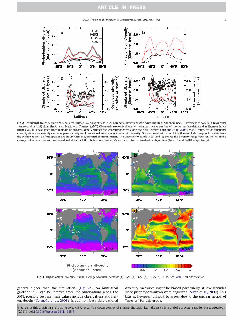
In the following, we discuss differences in simulated total phy-toplankton biomass, primary production (PP) and net community

a b

d e

Fig. 6. Primary production (PP). (a) Annual average PP (0–100 m depth) for LGNS is coaverages of PP are shown in (c) as absolute values and in (f) as absolute difference to LG

a b

d e

Fig. 7. Net community production (NCP). (a) Annual average NCP (0–100 m depth) for LGZonal averages of NCP are shown in (c) as absolute values and in (f) as absolute differen


production (NCP) between the different model configurations.NCP is defined as the difference between gross primary productionand community respiration within the euphotic zone. Interest-ingly, NCP is not only controlled bottom-up by physical transportprocesses supplying nutrients, but it also changes in response todifferent grazing parameterizations. In fact, the total phytoplank-ton biomass, PP and NCP differ by as much as a factor of two inthe annual mean among the different model simulations (Figs. 5–7; Table 1). The regional patterns of change relative to LGNS differbetween both low and high grazing switching setups. The effects ofswitching can be seen when comparing LGAS to LGNS. A detailed

c

f

mpared to (b) LGAS, (d) HGNS, and (e) HGAS as relative difference to LGNS. ZonalNS for all configurations.

c

f

NS is compared to (b) LGAS, (d) HGNS, and (e) HGAS as relative difference to LGNS.ce to LGNS for all configurations.




discussion of regional differences between configurations and theunderlying mechanisms is presented in Appendix C. In the follow-ing, we summarize the main findings.

For both LGAS and HGAS, total phytoplankton biomass and PP in-crease compared to LGNS and HGNS, respectively, in the productivehigher latitudes and in the tropics (shown for LGAS in Fig. 5b, Fig. 6b).For LGAS compared to LGNS, at higher latitudes higher uptake ofnutrients intensifies the vertical nutrient gradients. It thereby en-hances the mixing-driven input of nutrients from deeper layerswhich mostly fuels the PP increase. In combination with less grazing,higher phytoplankton biomass results, part of which is exported,thereby enhancing NCP. In contrast, in the permanently stratifiedlow latitude regions (25�S–25�N) dominated by small phytoplank-ton types, higher total phytoplankton biomass enhances a ‘‘fast recy-cling loop’’ via dissolved organic matter (DOM) which sustainshigher PP.

If grazing rates are increased (HGAS), a smaller phytoplanktonstanding stock leads to lower export, and thus lower NCP, in the

a

c

e

g

i

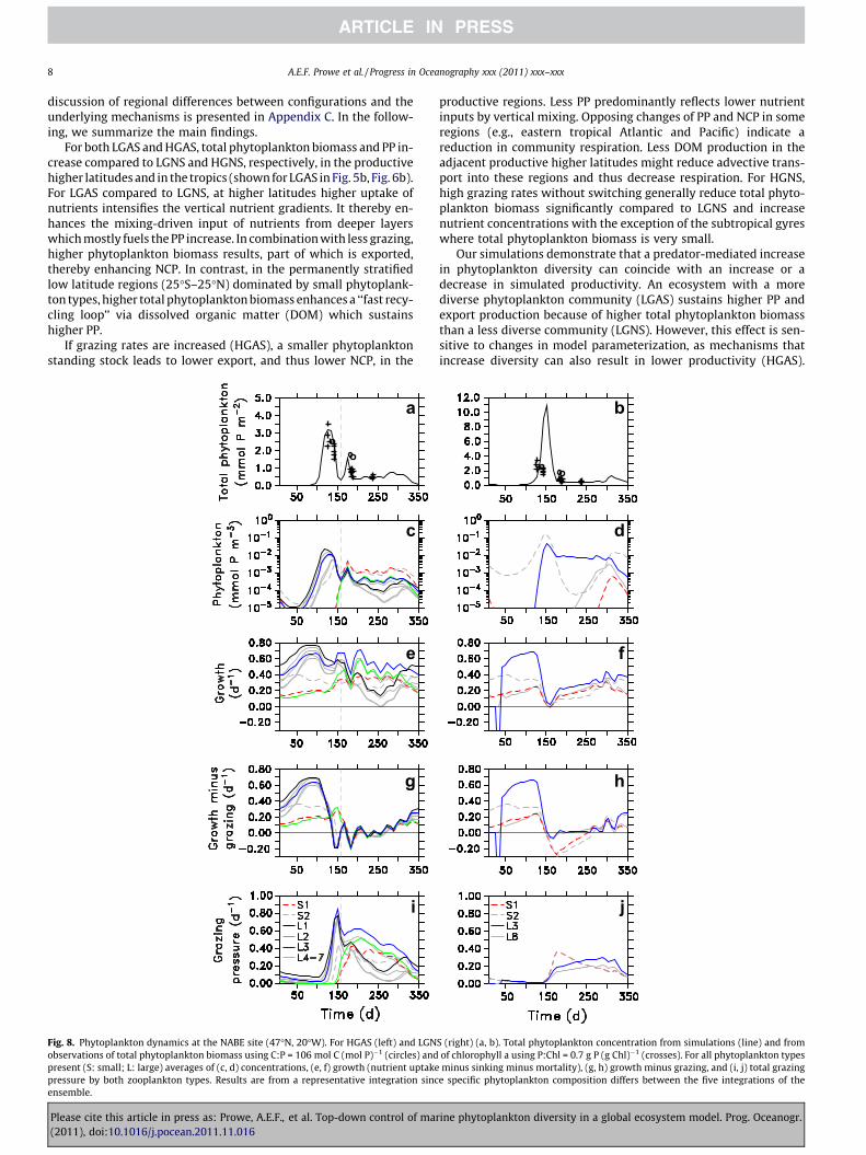
Fig. 8. Phytoplankton dynamics at the NABE site (47�N, 20�W). For HGAS (left) and LGNobservations of total phytoplankton biomass using C:P = 106 mol C (mol P)�1 (circles) andpresent (S: small; L: large) averages of (c, d) concentrations, (e, f) growth (nutrient uptakepressure by both zooplankton types. Results are from a representative integration sincensemble.


productive regions. Less PP predominantly reflects lower nutrientinputs by vertical mixing. Opposing changes of PP and NCP in someregions (e.g., eastern tropical Atlantic and Pacific) indicate areduction in community respiration. Less DOM production in theadjacent productive higher latitudes might reduce advective trans-port into these regions and thus decrease respiration. For HGNS,high grazing rates without switching generally reduce total phyto-plankton biomass significantly compared to LGNS and increasenutrient concentrations with the exception of the subtropical gyreswhere total phytoplankton biomass is very small.

Our simulations demonstrate that a predator-mediated increasein phytoplankton diversity can coincide with an increase or adecrease in simulated productivity. An ecosystem with a morediverse phytoplankton community (LGAS) sustains higher PP andexport production because of higher total phytoplankton biomassthan a less diverse community (LGNS). However, this effect is sen-sitive to changes in model parameterization, as mechanisms thatincrease diversity can also result in lower productivity (HGAS).

b

d

f

h

j

S (right) (a, b). Total phytoplankton concentration from simulations (line) and fromof chlorophyll a using P:Chl = 0.7 g P (g Chl)�1 (crosses). For all phytoplankton typesminus sinking minus mortality), (g, h) growth minus grazing, and (i, j) total grazing

e specific phytoplankton composition differs between the five integrations of the




Changes in productivity are fueled by differences in nutrientdistributions relative to the standard configuration, and thus differregionally depending on the physical regime. However, these dif-ferences reflect the state of the ecosystem after only short (10 year)integrations from the same initial conditions. Longer term adjust-ments within the ecosystem might modify the results.

The HGAS configuration reduces simulated differences in PPbetween eastern and western North Atlantic. This is potentiallyan improvement in the models results: Observational estimatesof PP at BATS (Bermuda Atlantic Time-series Study site) and atESTOC (European Station for Time series in the Ocean) show littledifference (0.38 vs. 0.4 g C m�2 d�1; Mouriño-Carballido andNeuer, 2008). On a global scale, however, the significance of thedifferences in PP and NCP is difficult to assess, as they are compa-rable with the uncertainties attached to the observational esti-mates. Differences in export production (not shown) between thedifferent configurations are comparable to differences found fordifferent multi-prey grazing formulations by Anderson et al.(2010). Our results support their study in confirming that multi-prey grazing functional responses have a large influence on simu-lated model dynamics. A more detailed comparison addressingphytoplankton community structure, specifically regarding theeffect of explicitly representing phytoplankton diversity withinplankton functional types, is to be reported elsewhere.

4.4. Seasonal phytoplankton dynamics

The seasonal pattern of simulated phytoplankton diversity isillustrated for the site of the North Atlantic Bloom Experiment(NABE), where active switching sustains a more diverse phyto-plankton community. For HGAS, the first phytoplankton springbloom is followed by a second, lower biomass peak and moderateconcentrations for the remainder of the year (Fig. 8a). This doublepeak agrees well with observed phytoplankton biomass (convertedfrom carbon to phosphorus units using C:P = 106 mol C (mol P)�1

or from chlorophyll a data using P:Chl = 0.7 g P (g Chl)�1). The firstpeak (days 100–150) is dominated by large phytoplankton typeswhich had high winter biomass (types L1, L3 in Fig. 8c) and highgrowth rates (Fig. 8e) in their environment. However, the type withthe highest concentration also feels the highest grazing pressure(G � Z, Fig. 8i), which reduces its growth more strongly than thatof other types (Fig. 8g) which then bloom consecutively. The sec-ond peak (day 175) is dominated by small phytoplankton typeswith lower maximum growth rates and higher nutrient affinity(S1, S2). Low grazing pressure allows them to survive the earlyspring and to finally displace the fast growing species (e.g. L1,L3) once nutrient concentrations decline at the end of the firstbloom peak. This succession of smaller types following the largertypes dominating the bloom is in good agreement with observa-tions at NABE (Lochte et al., 1993; Sieracki et al., 1993).

The active switching formulation suggests that phytoplanktonwhich achieve a biomass exceeding Pcrit may benefit from reducedspecific grazing pressure and thus potentially escape grazing con-trol. The Pcrit depends on the biomass of the other phytoplanktontypes (Eq. (10)) and is therefore a variable property of the phyto-plankton community. In particular, if many phytoplankton typescoexist and total biomass is high, it is more difficult for one typeto exceed the higher Pcrit than if total biomass is low. Furthermore,a concurrent increase in zooplankton biomass may offset a reduc-tion in specific grazing pressure. Within the bloom dynamics in ourmodel presented here, such effects are not immediately obvious.

In contrast to HGAS, the standard configuration (LGNS) producesonly one bloom peak (Fig. 8b) with one dominating small and onelarge phytoplankton type (Fig. 8d; S2 and L3, respectively). It overes-timates observed peak biomass by a factor of 3 for the conversion as-sumed (see caption of Fig. 8). Here again types with high winter


biomass (Fig. 8d) and high growth rates (Fig. 8f) dominate the peak.Without switching, grazing pressure is comparably high on all fourphytoplankton types present until the bloom peak (Fig. 8j) and thetypes less adapted to winter conditions (S1, L8) cannot survive thebloom in sufficient concentrations to take over afterwards. As a con-sequence of the lower grazing pressure at high food concentrations,the bloom peaks later and is more pronounced for LGNS compared toHGAS. The bloom is ended bottom up by nutrient limitation ongrowth rates and top-down effects are of minor importance(Fig. 8f and h). For LGAS, results are between those for LGNS andHGAS: the model simulates seasonal succession of 3 types duringthe first bloom peak, but overestimates observed phytoplanktonbiomass and captures only one bloom peak. HGNS yields abruptdynamics which seem unrealistic and overestimates observed phy-toplankton biomass to a larger extent than does LGNS.

In previous modeling studies at NABE, the double peak wasthought to result from co-limitation of diatoms by silicate (Fashamand Evans, 2000) or from single-phytoplankton-single-zooplank-ton interactions (Schartau and Oschlies, 2003). In our simulationswith active switching, the double peak is a consequence of a phy-toplankton community shift driven by both bottom-up and top-down mechanisms.

The simulated community dynamics at BATS mirror the differ-ences from configurations at NABE. At BATS, the bloom is lessclearly defined and total phytoplankton biomass is lower, butbroadly consistent with chlorophyll observations. For HGAS, twobloom peaks are formed through a succession of large and smallphytoplankton types, albeit less clearly than at NABE. For LGNS,one dominant phytoplankton type generates two less distinctbloom peaks. For both configurations, the bloom period is endedbottom-up by declining growth rates and top-down control bygrazing is not important during this time of the year.

5. Conclusions

Our results indicate that grazing pressure can be a key factor inshaping phytoplankton succession and community structure dur-ing blooms. Prey-ratio based predation, e.g. a type III or activeswitching formulation, increases diversity and better capturesthe observed phytoplankton succession. Significant changes in pri-mary and net community production occur between simulationswith different grazing formulations. Regional differences highlightthe role of recycling of organic matter in models. We have shownhere top-down mechanisms to have the potential for being essen-tial drivers of phytoplankton diversity in global ecosystem models.In addition to the ongoing attempts to relate phytoplankton diver-sity to physiological variances in the phytoplankton population,the intricate interplay between top-down and bottom-up controlson shaping marine phytoplankton diversity patterns will requiremore attention in future studies.

Role of the funding source

The funding sources had no involvement in study design, anal-ysis and interpretation of data, writing of the report or the decisionto submit the paper for publication.

Acknowledgements

FP gratefully acknowledges the technical help from Oliver Jahn.The authors thank Pedro Cermeño for providing data for hisobservational diversity estimate. Constructive comments by threeanonymous reviewers helped to improve the manuscript. FP issupported by the Kiel Cluster of Excellence ‘‘The Future Ocean’’.SD and MF acknowledge the support of the Gordon and Betty




Moore Foundation, the National Oceanic and Atmospheric Admin-istration, and the National Science Foundation.

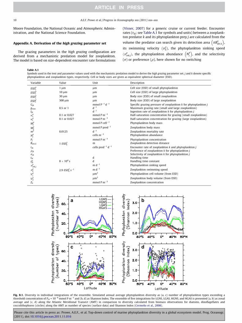
Appendix A. Derivation of the high grazing parameter set

The grazing parameters in the high grazing configuration arederived from a mechanistic predation model for zooplankton.The model is based on size-dependent encounter rate formulations

Table A.1Symbols used in the text and parameter values used with the mechanistic predaphytoplankton and zooplankton types, respectively. Cell or body sizes are give

Variable Value Unit

ESDPs

1 lm lm

ESDPl

10 lm lm

ESDZs

30 lm lm

ESDZl

300 lm lm

Gjk mmol P�1 d�1

gmax 0.5 or 1 d�1

Ijk d�1

jPs 0.1 or 0.027 mmol P m�3

jPl

0.1 or 0.027 mmol P m�3

MPj

mmol P cell�1

MZk

mmol P pred�1

mZ 0.0125 d�1

NPj

cells m�3

Pj mmol P m�3

Rdet,k 1 ESDZk

m

rjk cells pred�1 d�1

qjk

rjk

tH dt0

H8 � 104 s d

vPsnk;j

m d�1

vZk 2.9 ESDZ

k s�1 m d�1

VPj

lm3

VZk

lm3

Zk mmol P m�3

a

c

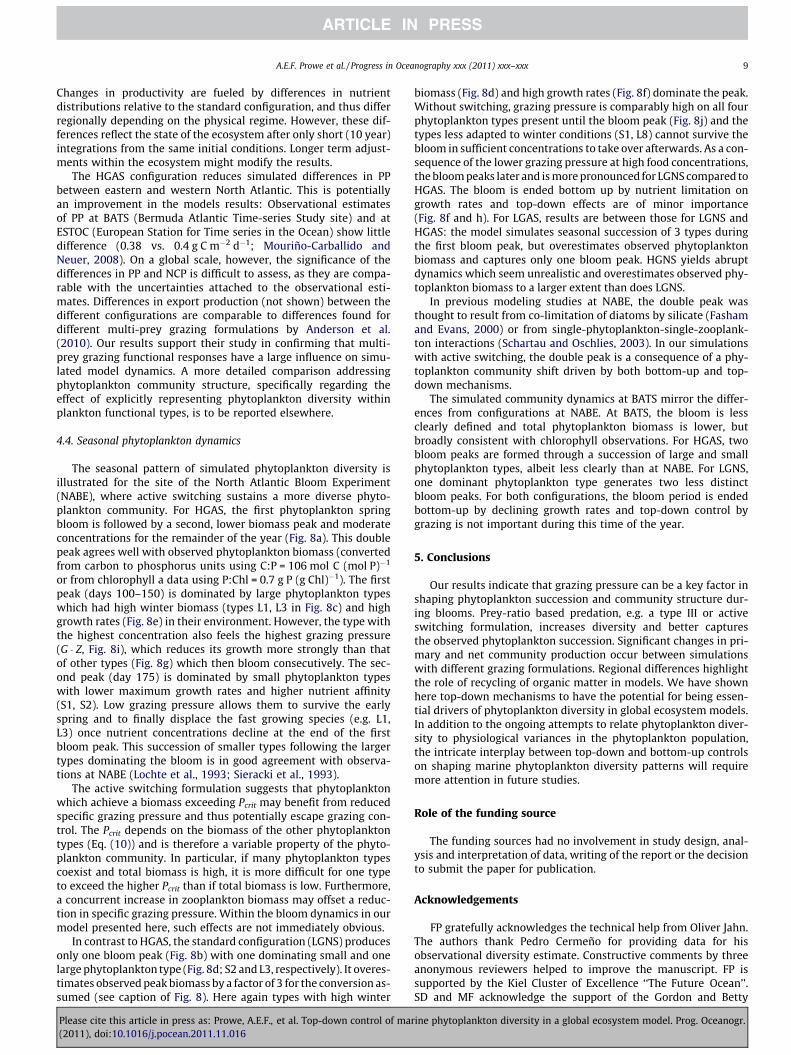
Fig. B.1. Diversity in individual integrations of the ensemble. Simulated annual averathreshold concentration of Pth = 10�8 mmol P m�3 and (b, d) as Shannon Index. The ensemaverage and (c, d) along the Atlantic Meridional Transect (AMT) in comparison tococcolithophores (circles) along the AMT as number of species (surface data) and Shann


(Visser, 2007) for a generic cruise or current feeder. Encounterrates (rkj; see Table A.1 for symbols and units) between a zooplank-ton predator k and its phytoplankton prey j are calculated from the

volume the predator can search given its detection area pR2det;k

� �,

its swimming velocity vZk

� �, the phytoplankton sinking speed

ðvPsnk;jÞ, the phytoplankton abundance NP

j

� �, and the selectivity

(r) or preference (q), here shown for no switching

tion model to derive the high grazing parameter set. j and k denote specificn as equivalent spherical diameter (ESD).

Description

Cell size (ESD) of small phytoplankton

Cell size (ESD) of large phytoplankton

Body size (ESD) of small zooplankton

Body size (ESD) of large zooplankton

Specific grazing pressure of zooplankton k for phytoplankton jMaximum grazing rate (small and large zooplankton)Ingestion rate of zooplankton k for phytoplankton jHalf-saturation concentration for grazing (small zooplankton)Half-saturation concentration for grazing (large zooplankton)

Phytoplankton body mass

Zooplankton body mass

Zooplankton mortality ratePhytoplankton abundance

Phytoplankton concentrationZooplankton detection distance

Encounter rate of zooplankton k and phytoplankton jPreference of zooplankton k for phytoplankton jSelectivity of zooplankton k for phytoplankton jHandling timeHandling time constantPhytoplankton sinking speed

Zooplankton swimming speed

Phytoplankton cell volume (from ESD)

Zooplankton body volume (from ESD)

Zooplankton concentration

b

d

ge phytoplankton diversity as (a, c) number of phytoplankton types exceeding able of five integrations for LGNS, LGAS, HGNS, and HGAS is presented (a, b) as zonal

diversity calculated from biomass observations for diatoms, dinoflagellates andon Index (Cermeño et al., 2008).




rkj ¼ pR2det;kqjkNP

j

ffiffiffiffiffiffiffiffiffiffiffiffiffiffiffiffiffiffiffiffiffiffiffiffiffiffivZ

k2 þ vP

snk;j2

q: ðA:1Þ

Detection distance (Rdet,k) and vZk are assumed to scale linearly with

predator size (expressed as equivalent spherical diameter ESDZk).

The vPsnk;j are interpolated from observations (Smayda, 1970).

The ingestion rate is calculated from the encounter rates con-sidering a handling time (tH) per successful encounter betweenpredator and prey

Ijk ¼MP

j

MZk

rkj

1þ tHrkj: ðA:2Þ

The handling time is set by the handling time constant t0H

� �and as-

sumed to vary proportionally with the predator–prey size ratio(MP

j =MZk; Pahlow and Prowe, 2010)

tH ¼ t0HMP

j =MZk : ðA:3Þ

Effects of turbulence, in the form of an additional turbulent velocityincreasing the encounter rates, are not considered here to enhancecomparability with the original predation model.

a

d

g

j

m

Fig. C.1. Differences in model dynamics between configurations. Fluxes between state vapanels: For LGNS, the black line represents the balance between source (positive) and silines are absolute changes relative to LGNS, with positive and negative values denotingpresented from top to bottom are phytoplankton (P), zooplankton (Z), nutrient (phosphatare primary production (N-P), sloppy feeding losses (P-OM (P-Z)), grazing (P-Z), phytoplaDOM (Z-DOM (Zm)) and POM (Z-POM (Zm)), recycling of DOM (DOM-N) and POM (POM-(P-DOM (P-Z) and P-POM (P-Z)), sinking of POM (POM sink). The black line in g shows thaPOM, and thus indicate physical supply by mixing.


The mechanistic predation model (Eqs. (A.1), (A.2)) reduces to atype II formulation for both active and no switching, here shownfor no switching

Ijk ¼1

tH0

qjkPj

MZk

tH0F þ qjkPj

; ðA:4Þ

where F ¼ pR2det;k

ffiffiffiffiffiffiffiffiffiffiffiffiffiffiffiffiffiffiffiffiffiffiffiffiffiffivZ

k2 þ vP

snk;j2

q. The maximum ingestion rate is gi-

ven by gmax ¼ 1=tH0 and the half-saturation concentration is

jPk ¼ MZ

k=ðtH0 FÞ. This qualitatively corresponds to the traditionalgrazing formulation implemented in the original model (Eq. (2)).

Parameters for the mechanistic predation model were estimatedfrom literature data. Zooplankton swimming speed generally in-creases with body size. For this application, vZ

k ¼ 2:9ESDZk s�1

according to data on different zooplankton groups ranging from4 lm ESD to 1.3 mm ESD (Hansen et al., 1997; Broglio et al.,2001; Strom and Morello, 1988; Tiselius and Jonsson, 1990). ThetH0 is set to yield a maximum ingestion rate of about 1 d�1 (Hansenet al., 1997), which is used for both the small and the largezooplankton type to be consistent with the original model. Bodymasses of phytoplankton and zooplankton (MP

j and MZk ,

b c

e f

h i

k l

n o

riables in the model are shown integrated over the top 100 m as zonal average. Leftnk (negative) fluxes. For LGAS and HGAS (middle and right panels, respectively), allincreases and decreases of the respective flux. State variables for which fluxes aree; N), dissolved organic matter (DOM) and particulate organic matter (POM). Fluxesnkton mortality (P-OM (Pm)), phytoplankton sinking (P sink), zooplankton losses toN) from phytoplankton mortality (P-DOM (Pm) and P-POM (Pm)) and sloppy feedingt nutrients taken up by phytoplankton cannot be supplied by recycling of DOM and




respectively) are calculated from volumes (VPj and VZ

k , respectively)based on cell or body size (ESD) for phytoplankton (Menden-Deuerand Lessard, 2000)

MPj ½pg C� ¼ 0:288 � VP

J ½lm3�0:811 ðA:5Þ

and for zooplankton (Verity and Langdon, 1984)

MZk ½pg C� ¼ 0:445þ 0:053 � VZ

k ½lm3� ðA:6Þ

and converted to model units (mmol P cell�1) using Redfield stoichi-ometry. The detection distance is set to Rdet;k ¼ 1ESDZ

k for simplicity,which is within the range of values calculated for hydromechanicaldetection of different types of prey (Visser, 2001). While for the lowgrazing configurations gmax = 0.5 d�1 and jP

k ¼ 0:1 mmol P m�3

(Table 1), the above parameter choices for the mechanistic modelimply gmax = 1 d�1 and jP

k ¼ 0:027 mmol P m�3, thus generallyresulting in higher ingestion rates in the high grazing configurations.Differences in jP

k arising from the different size of the two zooplank-ton types (cf. Table A.1) are negligible and an intermediate jP

k isemployed for both zooplankton types in accordance with the originalmodel.

Appendix B. Diversity between different integrations of theensemble

Results presented in this study are the average of an ensembleof five integrations each with a different set of phytoplanktonparameters randomly chosen within a given range. Phytoplanktondiversity differs only slightly between different integrations(Fig. B.1). The geographical patterns for all integrations (notshown) are similar and differ less between integrations with thesame configuration than between different configurations.

Appendix C. Changes in primary production and net communityproduction between configurations

For both LGAS and HGAS, total phytoplankton biomass and PPincrease compared to LGNS and HGNS, respectively, in the produc-tive higher latitudes and in the tropics (shown for LGAS in Fig. 5b,Fig. 6b). For LGAS, in higher latitudes lower nutrient concentrationsin the surface mixed layer (not shown) lead to a stronger verticalnutrient gradient, and thereby cause higher input of nutrientsfrom the deeper layers by processes like deep winter mixing(Fig. C.1h). This enhanced nutrient input fuels the largest part ofthe PP increase, while only a small fraction is due to higherrecycling of dissolved organic matter (DOM). Together with lessgrazing (Fig. C.1e), higher total phytoplankton biomass remains(Fig. C.1b). In contrast, in the permanently stratified low latitude re-gions (25�S–25�N) with little nutrient input by vertical eddydiffusion, enhanced recycling of DOM via phytoplankton mortalityis mostly responsible for higher PP and appears to enhance a ‘‘fastrecycling loop’’ (Fig. C.1h). With switching, the damped growth ofdominant types and the reduced grazing pressure on phytoplank-ton types less successful in the competition for nutrients allowsthe latter types to grow, albeit slowly, at low nutrient concentra-tions. This increases not only diversity, but also total phytoplanktonbiomass. At higher latitudes, a fraction of this phytoplankton bio-mass is exported to greater depths as particulate organic matter(POM; Fig. C.1n) which is thus not available for remineralizationin the surface layer but enhances NCP instead (Fig. 7). The lowerlatitudes are dominated by small phytoplankton types, for whichhigher mortality leads to more DOM but little more POM(Figs. C1k and n). If grazing rates are increased (HGAS), the phyto-plankton standing stock is reduced compared to LGAS, causing low-er recycling of nutrients via phytoplankton mortality (Fig. C1c). Thesimultaneous decrease in PP, however, predominantly reflects low-


er nutrient inputs by vertical mixing caused by higher nutrient con-centrations in the surface layer (Fig. C.1i). Lower phytoplanktonmortality also leads to lower export of POM, and thus lower NCP(Fig. 7), in the productive regions, and is only partly compensatedby increased fecal pellet production by the zooplankton (Fig. C.1o).

References

Aiken, J., Pradhan, Y., Barlow, R., Lavender, S., Poulton, A., Holligan, P., Hardman-Mountford, N., 2009. Phytoplankton pigments and functional types in theAtlantic Ocean: a decadal assessment, 1995–2005. Deep-Sea Research Part II –Topical Studies In Oceanography 56, 899–917.

Anderson, T.R., Gentleman, W.C., Sinha, B., 2010. Influence of grazing formulationson the emergent properties of a complex ecosystem model in a global Oceangeneral circulation model. Progress in Oceanography 87, 201–213.

Aumont, O., Bopp, L., 2006. Globalizing results from Ocean in situ iron fertilizationstudies. Global Biogeochemical Cycles 20. doi:10.1029/2005GB002591.

Aumont, O., Maier-Reimer, E., Blain, S., Monfray, P., 2003. An ecosystem model ofthe global Ocean including Fe, Si, P colimitations. Global Biogeochemical Cycles17. doi:10.1029/2001GB001745.

Barton, A.D., Dutkiewicz, S., Flierl, G., Bragg, J., Follows, M.J., 2010. Patterns ofdiversity in marine phytoplankton. Science 327, 1509–1511.

Bopp, L., Aumont, O., Cadule, P., Alvain, S., Gehlen, M., 2005. Response of diatomsdistribution to global warming and potential implications: A global modelstudy. Geophysical Research Letters 32. doi:10.1029/2005GL023653.

Boyd, P., Doney, S., 2002. Modelling regional responses by marine pelagicecosystems to global climate change. Geophysical Research Letters 29.doi:10.1029/2001GL014130.

Broglio, E., Johansson, M., Jonsson, P.R., 2001. Trophic interaction between copepodsand ciliates: Effects of prey swimming behavior on predation risk. MarineEcology Progress Series 220, 179–186.

Bruggeman, J., Kooijman, S.A.L.M., 2007. A biodiversity-inspired approach to aquaticecosystem modeling. Limnology and Oceanography 52, 1533–1544.

Cardinale, B.J., Srivastava, D.S., Duffy, J.E., Wright, J.P., Downing, A.L., Sankaran, M.,Jouseau, C., 2006. Effects of biodiversity on the functioning of trophic groupsand ecosystems. Nature 443, 989–992.

Cermeño, P., Marañón, E., Harbour, D., Figueiras, F.G., Crespo, B.G., Huete-Ortega, M.,Varela, M., Harris, R.P., 2008. Resource levels, allometric scaling of populationabundance, and marine phytoplankton diversity. Limnology and Oceanography53, 312–318.

Chase, J., Abrams, P., Grover, J., Diehl, S., Chesson, P., Holt, R., Richards, S., Nisbet, R.,Case, T., 2002. The interaction between predation and competition: a reviewand synthesis. Ecology Letters 5, 302–315.

Chesson, P., 2000. Mechanisms of maintenance of species diversity. Annual Reviewof Ecology and Systematics 31, 343–366.

Duffy, J., Stachowicz, J., 2006. Why biodiversity is important to Oceanography:potential roles of genetic, species, and trophic diversity in pelagic ecosystemprocesses. Marine Ecology Progress Series 311, 179–189.

Dutkiewicz, S., Follows, M.J., Bragg, J.G., 2009. Modeling the coupling of Oceanecology and biogeochemistry. Global Biogeochemical Cycles 23. doi:10.1029/2008GB003405.

Fasham, M., Ducklow, H., McKelvie, S., 1990. A nitrogen-based model of planktondynamics in the Oceanic mixed layer. Journal of Marine Research 48, 591–639.

Fasham, M., Sarmiento, J., Slater, R., Ducklow, H., Williams, R., 1993. Ecosystembehavior at Bermuda Station-S and Ocean Weather Station India - A General-circulation model and observational analysis. Global Biogeochemical Cycles 7,379–415.

Fasham, M.J.R., Evans, G.T., 2000. Advances in ecosystem modelling within JGOFS.In: Hanson, R.B., Ducklow, H.W., Field, J.G. (Eds.), The Changing Ocean CarbonCycle. Cambridge University Press, pp. 417–446.

Follows, M.J., Dutkiewicz, S., Grant, S., Chisholm, S.W., 2007. Emergentbiogeography of microbial communities in a model Ocean. Science 315,1843–1846.

Gentleman, W., Leising, A., Frost, B., Strom, S., Murray, J., 2003. Functional responsesfor zooplankton feeding on multiple resources: A review of assumptions andbiological dynamics. Deep-Sea Research Part II 50, 2847–2875.

Gentleman, W.C., Neuheimer, A.B., 2008. Functional responses and ecosystemdynamics: How clearance rates explain the influence of satiation, food-limitation and acclimation. Journal of Plankton Research 30, 1215–1231.

Gross, T., Edwards, A.M., Feudel, U., 2009. The invisible niche: Weakly density-dependent mortality and the coexistence of species. Journal of TheoreticalBiology 258, 148–155.

Hansen, P.J., Bjørnsen, P.K., Hansen, B.W., 1997. Zooplankton grazing and growth:Scaling within the 2-2,000-lm body size range. Limnology and Oceanography42, 687–704.

Hutchinson, G.E., 1961. The paradox of the plankton. The American Naturalist 95,137–145.

Hutson, V., 1984. Predator mediated coexistence with a switching predator.Mathematical Biosciences 68, 233–246.

Jonsson, P.R., Tiselius, P., 1990. Feeding behaviour, prey detection and captureefficiency of the copepod Acartia tonsa feeding on planktonic ciliates. MarineEcology Progress Series 60, 35–44.

Kiørboe, T., Saiz, E., Viitasalo, M., 1996. Prey switching behaviour in the planktoniccopepod Acartia tonsa. Marine Ecology Progress Series 143, 65–75.


http://dx.doi.org/10.1029/2005GB002591

http://dx.doi.org/10.1029/2001GB001745

http://dx.doi.org/10.1029/2005GL023653

http://dx.doi.org/10.1029/2001GL014130

http://dx.doi.org/10.1029/2008GB003405

http://dx.doi.org/10.1029/2008GB003405



Le Quéré, C., Harrison, S., Prentice, I., Buitenhuis, E., Aumont, O., Bopp, L., Claustre,H., Cotrim Da Cunha, L., Geider, R., Giraud, X., Klaas, C., Kohfeld, K., Legendre, L.,Manizza, M., Platt, T., Rivkin, R., Sathyendranath, S., Uitz, J., Watson, A., Wolf-Gladrow, D., 2005. Ecosystem dynamics based on plankton functional types forglobal Ocean biogeochemistry models. Global Change Biology 11, 2016–2040.

Levin, S.A., 1970. Community equilibria and stability, and an extension of thecompetitive exclusion principle. American Naturalist 104, 413–423.

Lochte, K., Ducklow, H., Fasham, M., Stienen, C., 1993. Plankton succession andcarbon cycling at 47�N-20�W during the JGOFS North-Atlantic BloomExperiment. Deep-Sea Research Part II – Topical Studies In Oceanography 40,91–114.

Manizza, M., Buitenhuis, E.T., Le Quéré, C., 2010. Sensitivity of global Oceanbiogeochemical dynamics to ecosystem structure in a future climate.Geophysical Research Letters 37. doi:10.1029/2010GL043360.

Mariani, P., Visser, A.W., 2010. Optimization and emergence in marine ecosystemmodels. Progress in Oceanography 84, 89–92.

Menden-Deuer, S., Lessard, E.J., 2000. Carbon to volume relationships fordinoflagellates, diatoms, and other protist plankton. Limnology andOceanography 45, 569–579.

Merico, A., Bruggeman, J., Wirtz, K., 2009. A trait-based approach for downscalingcomplexity in plankton ecosystem models. Ecological Modelling 220, 3001–3010.

Morán, X.A.G., López-Urrutia, A., Calvo-Díaz, A., Li, W.K.W., 2010. Increasingimportance of small phytoplankton in a warmer Ocean. Global ChangeBiology 16, 1137–1144.

Mouriño-Carballido, B., Neuer, S., 2008. Regional differences in the role of eddypumping in the North Atlantic Subtropical Gyre – historical conundrumsrevisited. Oceanography 21, 52–61.

Murdoch, W.W., Oaten, A., 1975. Predation and population stability. Advances inEcological Research 9, 1–131.

Norberg, J., 2004. Biodiversity and ecosystem functioning: A complex adaptivesystems approach. Limnology and Oceanography 49, 1269–1277.

Paffenhöfer, G.A., 1984. Food ingestion by the marine planktonic copepodParacalanus in relation to abundance and size distribution of food. MarineBiology 80, 323–333.

Pahlow, M., Prowe, A.E.F., 2010. Model of zooplankton optimal current feeding.Marine Ecology Progress Series 403, 129–144.

Prowe, A.E.F., Pahlow, M., Oschlies, A., 2012. Controls on the diversity-productivityrelationship in a marine ecosystem model. Ecological Modelling 225, 167–176.

Ptacnik, R., Moorthi, S.D., Hillebrand, H., 2010. Hutchinson reversed, or why thereneed to be so many species. Advances in Ecological Research 43, 1–43.

Ptacnik, R., Solimini, A.G., Andersen, T., Tamminen, T., Brettum, P., Lepisto, L., Willén,E., Rekolainen, S., 2008. Diversity predicts stability and resource use efficiencyin natural phytoplankton communities. In: Proceedings of the NationalAcademy of Sciences of the United States of America, vol. 105, pp. 5134–5138.

Roy, S., Chattopadhyay, Y., 2007. Towards a resolution of ‘the paradox of theplankton’: a brief overview of proposed mechanisms. Ecological Complexity 4,26–33.


Saiz, E., Kiørboe, T., 1995. Predatory and suspension feeding of the copepod Acartiatonsa in turbulent environments. Marine Ecology Progress Series 122,147–158.

Schartau, M., Oschlies, A., 2003. Simultaneous data-based optimization of a 1D-ecosystem model at three locations in the North Atlantic: Part II – standingstocks and nitrogen fluxes. Journal of Marine Research 61, 795–821.

Sieracki, M., Verity, P., Stoecker, D., 1993. Plankton community response tosequential silicate and nitrate depletion during the 1989 North-Atlanticspring bloom. Deep-Sea Research Part II – Topical Studies In Oceanography40, 213–225.

Smayda, T.J., 1970. The suspension and sinking of phytoplankton in the sea.Oceanography and Marine Biology: An Annual Review 8, 353–414.

Stirling, G., Wilsey, B., 2001. Empirical relationships between species richness,evenness, and proportional diversity. American Naturalist 158, 286–299.

Strom, S.L., Miller, C.B., Frost, B.W., 2000. What sets lower limits to phytoplanktonstocks in high-nitrate, low-chlorophyll regions of the open Ocean? MarineEcology Progress Series 193, 19–31.

Strom, S.L., Morello, T.A., 1988. Comparative growth rates and yields of ciliates andheterotrophic dinoflagellates. Journal of Plankton Research 20, 571–584.

Tilman, D., Lehman, C., Thomson, K., 1997. Plant diversity and ecosystemproductivity: theoretical considerations. In: Proceedings of the NationalAcademy of Sciences of the United States of America, vol. 94, pp. 1857–1861.

Tiselius, P., Jonsson, P.R., 1990. Foraging behaviour of six calanoid copepods:observations and hydrodynamic analysis. Marine Ecology Progress Series 66,23–33.

Verity, P.G., Langdon, C., 1984. Relationships between lorica volume, carbon,nitrogen, and ATP content of tintinnids in Narragansett Bay. Journal of PlanktonResearch 6, 859–868.

Visser, A.W., 2001. Hydromechanical signals in the plankton. Marine EcologyProgress Series 222, 1–24.

Visser, A.W., 2007. Motility of zooplankton: fitness, foraging and predation. Journalof Plankton Research 29, 447–461.

Worm, B., Barbier, E.B., Beaumont, N., Duffy, J.E., Folke, C., Halpern, B.S., Jackson,J.B.C., Lotze, H.K., Micheli, F., Palumbi, S.R., Sala, E., Selkoe, K.A., Stachowicz, J.J.,Watson, R., 2006. Impacts of biodiversity loss on Ocean ecosystem services.Science 314, 787–790.

Worm, B., Lotze, H., Hillebrand, H., Sommer, U., 2002. Consumer versus resourcecontrol of species diversity and ecosystem functioning. Nature 417, 848–851.

Wunsch, C., Heimbach, P., 2007. Practical global Oceanic state estimation. Physica D– Nonlinear Phenomena 230, 197–208.

Yachi, S., Loreau, M., 1999. Biodiversity and ecosystem productivity in a fluctuatingenvironment: the insurance hypothesis. In: Proceedings of the NationalAcademy of Sciences of the United States of America, vol. 96, pp. 1463–1468.

Yool, A., Popova, E.E., Anderson, T.R., 2011. MEDUSA: a new intermediatecomplexity plankton exosystem model for the global domain. GeoscientificModel Development 4, 381–417.


http://dx.doi.org/10.1029/2010GL043360


Documents

Progress in Oceanography - Massachusetts Institute of …ocean.mit.edu/~stephd/proweetal_progoce_2011.pdf · 2016-06-05 · Top-down control of marine phytoplankton diversity in a