Progress report: Development of assessment and predictive metrics for quantitative imaging in

chest CT

Subaward No: HHSN268201000050C (4a)

PI: Ehsan Samei

Reporting Period: month 1-18

Deliverables:

1. Deployment of a framework for drawing a correspondence between simple figure of merits

(FOM) and quantitative imaging performance in CT.

A surrogate of quantification precision, named estimability index (e’), was developed by

incorporating information from three aspects: 1) the resolution (task transfer function, TTF)

and noise (noise power spectrum, NPS) property of the imaging system, 2) the characteristics

of the nodule to be quantified (task function, Wtask), and 3) the stability of the segmentation

software (internal noise, Ni).

Noise Property The noise property of the system was characterized in terms of 3D NPS,

using the uniform region in Module 3 of ACR CT accreditation phantom (Gammex 464). To

capture possible shift of frequency components as observed in iterative reconstructions, the

NPS was measured at multiple noise levels by rescanning the phantom at various dose levels.

Resolution Property The resolution property was characterized in terms of 3D TTF, using

the circular and the plane edges of the cylindrical inserts of various attenuations in Module 1

of ACR Phantom. TTF was an extension of the concept of modulation transfer function

(MTF) to accommodate the nonlinearity of iterative reconstruction within a narrow,

linearizable operating band (i.e., specific object contrast and noise levels). To fully capture

the whole operating space, a range of TTF values were acquired at various contrast and noise

levels. Multiple steps were incorporated to ensure a robust and reliable measurement of TTF

with low object contrast and high image noise, as illustrated in Figure 1. Examples of

measured NPS and TTF are shown in Figure 2.

Figure 1: (a,b) The TTF in XOY-plane is calculated with the circular edge of the insert, from which

the edge spread function (ESF) can be formed by plotting the intensity of all pixels within the ROI

against their distance from the center of the insert. (c,d) The TTF along the z-direction is calculated

with the angled plane edge at the end of the insert, from which the ESF can be formed by plotting the

intensity of all pixels within the ROI against their distance from the edge. (e,f,g,h,i) The same

technique was applied to acquire XOY- or z-TTF from the ESF through a series of de-noise

processing.

Figure 2: Examples of (a) 3D NPS and (b) 3D TTF. (c) TTF of iterative reconstructions shows a strong

dependency on the noise, which was reflected in the e’ calculations.

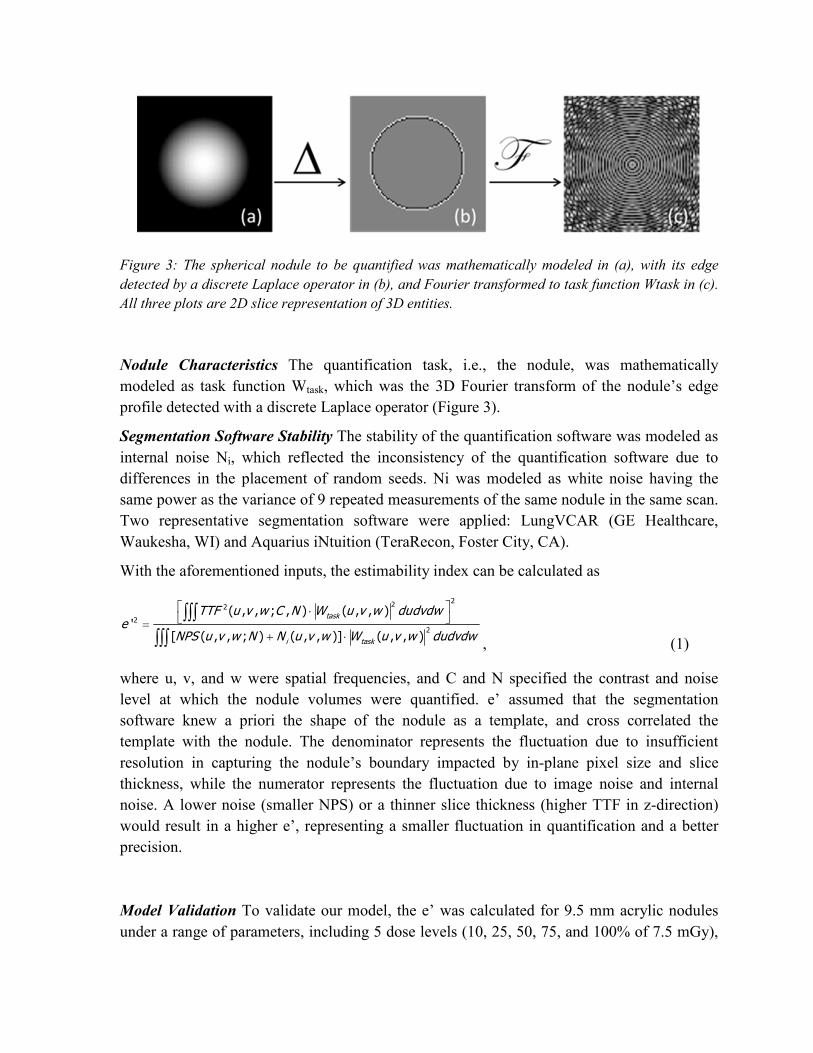
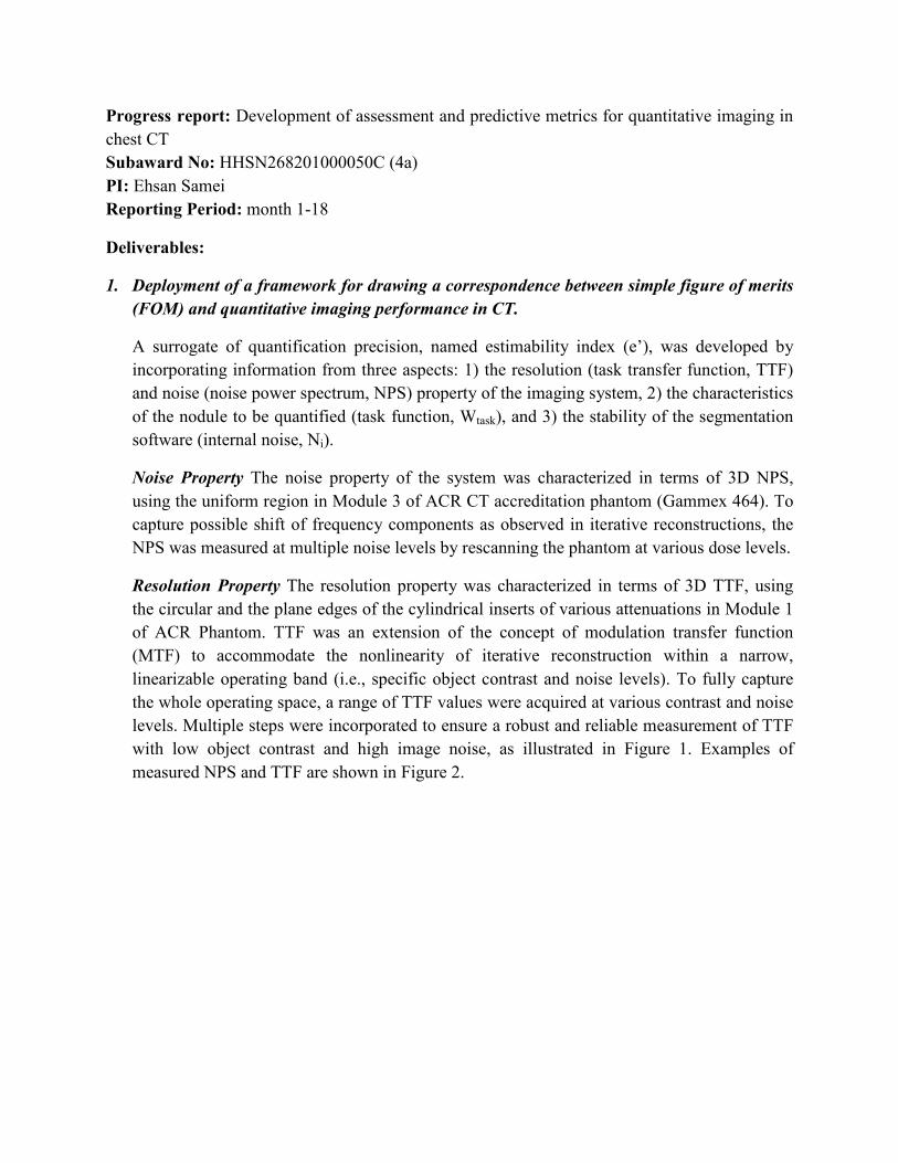
Figure 3: The spherical nodule to be quantified was mathematically modeled in (a), with its edge

detected by a discrete Laplace operator in (b), and Fourier transformed to task function Wtask in (c).

All three plots are 2D slice representation of 3D entities.

Nodule Characteristics The quantification task, i.e., the nodule, was mathematically

modeled as task function Wtask, which was the 3D Fourier transform of the nodule’s edge

profile detected with a discrete Laplace operator (Figure 3).

Segmentation Software Stability The stability of the quantification software was modeled as

internal noise Ni, which reflected the inconsistency of the quantification software due to

differences in the placement of random seeds. Ni was modeled as white noise having the

same power as the variance of 9 repeated measurements of the same nodule in the same scan.

Two representative segmentation software were applied: LungVCAR (GE Healthcare,

Waukesha, WI) and Aquarius iNtuition (TeraRecon, Foster City, CA).

With the aforementioned inputs, the estimability index can be calculated as

222

2

2

( , , ; , ) ( , , )'

[ ( , , ; ) ( , , )] ( , , )

task

i task

TTF u v w C N W u v w dudvdwe

NPS u v w N N u v w W u v w dudvdw

⋅ =

+ ⋅

∫∫∫

∫∫∫ , (1)

where u, v, and w were spatial frequencies, and C and N specified the contrast and noise

level at which the nodule volumes were quantified. e’ assumed that the segmentation

software knew a priori the shape of the nodule as a template, and cross correlated the

template with the nodule. The denominator represents the fluctuation due to insufficient

resolution in capturing the nodule’s boundary impacted by in-plane pixel size and slice

thickness, while the numerator represents the fluctuation due to image noise and internal

noise. A lower noise (smaller NPS) or a thinner slice thickness (higher TTF in z-direction)

would result in a higher e’, representing a smaller fluctuation in quantification and a better

precision.

Model Validation To validate our model, the e’ was calculated for 9.5 mm acrylic nodules

under a range of parameters, including 5 dose levels (10, 25, 50, 75, and 100% of 7.5 mGy),

3 reconstruction algorithms (FBP and 2 iterative reconstructions, ASIR, and MBIR), and 3

slice thicknesses (0.625, 1.25, and 2.5 mm), yielding 45 protocols in total. The e’ was then

compared against empirical precision in terms of percent repeatability coefficient (PRC),

which was measured under the same 45 protocols via an anthropomorphic phantom with

synthetic nodules [1, 2]. PRC was defined as the expected absolute difference between any

two repeated quantifications of the same object normalized by the true nodule volume, for 95%

of cases. A higher PRC represents larger fluctuation in quantifications. For jth protocol with

n nodules and K repetitions, PRC was calculated as

_2 2

1 1

1.96 2 2.77 ( )2.77 /

( 1)

Wj j ijk ijn Kj i k true

true true

WMS V VPRC V

V V n K

σ= =

−= ≈ =

−∑ ∑ . (2)

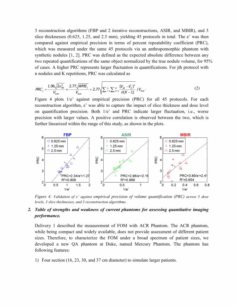
Figure 4 plots 1/e’ against empirical precision (PRC) for all 45 protocols. For each

reconstruction algorithm, e’ was able to capture the impact of slice thickness and dose level

on quantification precision. Both 1/e’ and PRC indicate larger fluctuation, i.e., worse

precision with larger values. A positive correlation is observed between the two, which is

further linearized within the range of this study, as shown in the plots.

Figure 4: Validation of e’ against empirical precision of volume quantification (PRC) across 5 dose

levels, 3 slice thicknesses, and 3 reconstruction algorithms.

2. Table of strengths and weakness of current phantoms for assessing quantitative imaging

performance.

Delivery 1 described the measurement of FOM with ACR Phantom. The ACR phantom,

while being compact and widely available, does not provide assessment of different patient

sizes. Therefore, to characterize the FOM under a broad spectrum of patient sizes, we

developed a new QA phantom at Duke, named Mercury Phantom. The phantom has

following features:

1) Four section (16, 23, 30, and 37 cm diameter) to simulate larger patients.

2) Four 1’’ cylindrical inserts (acrylic, air, Teflon, and polyethylene; 120, -1000, 900, -50

HU @ 120 kVp) and four 0.5’’ iodinated inserts (2.2, 4.3, 6.4, and 8.5 mg/cc; 25, 96, 164,

and 224 HU @ 120 kVp) in each section to capture TTF’s dependency on contrast.

3) Uniform region in each section to capture NPS.

Figure 5: The phantom developed at Duke allows size-specific measurements of 3D

FOM.

Table 1 summarizes the strength and weakness of ACR and Mercury Phantoms in assessing

3D FOMs for quantification precision. The strengths are color-coded in green and the

weaknesses are coded in red. Overall, Mercury Phantom has more strengths than ACR

Phantom, but still has space for future improvements.

Table 1: Strengths and weakness of ACR and Mercury Phantoms in assessing quantification

precision.

ACR Phantom Mercury Phantom

TTF

measurement

The four 1’’ inserts only provide three

contrast levels (air and bone inserts

have similar absolute contrast), not

sufficient to characterize the entire

operating space.

The four 1’’ inserts provide two high and

two low contrast levels. The four ½’’

inserts provide additional low-to-medium

contrast levels to help characterize the

operating space.

The circular edges at the side of the Occasional air gap were observed between

cylindrical inserts are perfectly glued

with the rest of the phantom, leaving

no air gap in between.

the insert and the phantom body, which

can be eliminated by improving

manufacture in future.

The plane edges at the two ends of the

cylindrical insert are not fully polished

for TTF measurements along the axial

direction.

The plane edge is fully polished for TTF

measurements along the axial direction.

High contrast wedges in between of

inserts affect the sharpness of the edge

to unknown extent.

No unnecessary components except a low

contrast, thin rod in the center of the

phantom to combine all sections.

NPS

measurement

Only one size (20 cm)

Four sizes (16, 23, 30, and 37 cm) to

capture the impact of patient size on noise

texture and magnitude.

High contrast BBs affect the image

uniformity to an unknown extent

Most region is uniform except a low

contrast, thin rod in the center of the

phantom to combine all sections.

Phantom

setup

Light Heavy

Compact Require assembly

3. Identify tolerances and threshold that CT quantification requires in terms of FOM

measured on QA phantoms and recommend guidelines for compliance

of quantitation techniques (software and hardware).

Based on Deliverable 1 and 2, a guideline for phantom-based assessment of quantification

precision is summarized in Table 2. It allows indirect calculation of PRC for a range of

protocols with limited number of scans, delivered in two phases. Only Phase 1 involves scans

of the ACR Phantom that characterizes the operating space. PRC of any protocol within the

operating space characterized in Phase 1 can be calculated in Phase 2, with respect to the

nodule characteristics and the segmentation software of interest.

Table 2: Guideline for phantom-based assessment of quantification precision for given combinations

of protocol, nodule characteristic, and segmentation software.

Phase 1 Step 1

ACR/Mercury Phantom or equivalent that contains

- cylindrical inserts of various attenuations for 3D TTF measurements

- uniform region for 3D NPS measurements

Scan the phantom with a range of dose levels and reconstruct it with multiple

slice thicknesses and reconstruction algorithms to compute a library of 3D

TTF and NPS values that characterize the entire operating space

Phase 2 Step 2

Model Wtask according to the size, shape, and contrast of the nodule being

assessed

Model Ni according to the quantification software being assessed

Step 3 Interpolate a 3D TTF from the library built in Step 1 with respect to the

nodule’s contrast and the image noise of the protocol (imaging and

reconstruction parameters) being assessed. This is especially important for

protocols involving iterative reconstructions.

Interpolate a 3D NPS from the library with respect to the image noise of the

protocol

Step 4 Incorporate TTF, NPS, Wtask and Ni into calculating e’ for the

aforementioned combination of nodule, segmentation software, and protocol

Step 5

Relate e’ to PRC

PRC = 2.34/e’+1.27 (FBP)

PRC = 2.96/e’+2.15 (ASIR)

PRC = 3.89/e’+2.41 (MBIR)

Finally, compare PRC to a threshold level and make suggestions

As a demonstration of our e’ model’s utility in guiding compliance of quantitation techniques,

this recipe was further used to predict the PRC of nodules ranging from 3 to 15 mm under a

number of protocols, as shown in Figure 6Error! Reference source not found.. The PRC

values were then compared to a threshold level to demonstrate the usage of our methodology

in guiding compliance of quantification techniques. For example, using 5% precision as a

threshold, the quantification of 5 mm nodules with FBP reconstruction requires a slice

thickness thinner than or equal to 1.25 mm, and a dose higher than or equal to 4 mGy.

Figure 6: PRC values predicted for 4.8 mm nodule from our e’ model.

Publications:

1. Chen B, Richard S, Barnhart H, Colsher J, Amurao M, Samei E. Quantitative CT:

technique dependency of volume assessment for pulmonary nodules. Physics in Medicine

and Biology 57: 1335–1348, 2012.

2. Chen B, Richard S, Samei E. Relevance of MTF and NPS in quantitative CT: towards

developing a predictable model of quantitative performance. SPIE International Symposium

on Medical Imaging, San Diego, CA, February 2012, Proc. SPIE Medical Imaging, 2012.

Presentations/Abstracts:

1. Richard S, Chen B, Samei E, et al. A novel method for predicting the performance of lung

nodule volume estimation in CT via ACR phantom measurements. Proceedings of the

Scientific Assembly and Annual Meeting of the Radiological Society of North America,

Chicago, IL, Dec. 2011, RSNA’11.

2. Wilson J M, Christianson O I, Chen B, Winslow J, Samei E, "mA Modulation and Iterative

Reconstruction: Evaluation Using a New CT Phantom," AAPM Annual Meeting, oral

presentation, 2012.

Work to be presented:

1. Chen B, Samei E. Development of a phantom-based methodology for the assessment of

quantification performance. Feb. 2013, SPIE Medical Imaging.