Progressive Taxation as an Automatic Stabilizerunder Nominal Wage Rigidity and Preference

Shocks∗

Miroslav GabrovskiUniversity of Hawaii at Manoa†

Jang-Ting GuoUniversity of California, Riverside‡

March 1, 2021

Abstract

Previous research has shown that in the context of a prototypical New Keynesian model,more progressive income taxation may lead to higher volatilities of hours worked and totaloutput in response to a monetary disturbance. We analytically show that this business-cycle destabilization result is overturned within an otherwise identical macroeconomy sub-ject to impulses to the household’s utility formulation. Under a continuously or linearlyprogressive fiscal policy rule with the symmetric-equilibrium tax burden unchanged, anincrease in the positive level of tax progressivity will always raise the degree of equilibriumnominal-wage rigidity, and thus serve as an automatic stabilizer that mitigates cyclicalfluctuations driven by preference shocks.

Keywords: Progressive Income Taxation, Automatic Stabilizer, Nominal Wage Rigidity,Preference Shocks.

JEL Classification: E12, E32, E62.

∗We thank Yuichi Furukawa (Managing Editor), an Associate Editor, two anonymous referees, NicolasCaramp, Juin-Jen Chang, Mingming Jiang, Yi Mao, Victor Ortego-Marti, Chong-Kee Yip, and seminar partic-ipants at Academia Sinica, Chinese University of Hong Kong, Chinese University of Hong Kong at Shenzhan,Shadong University, and National Chengchi University for helpful comments and suggestions. Part of this re-search was conducted while Guo was a visiting research fellow at the Institute of Economics, Academia Sinica,whose hospitality is greatly appreciated. Of course, all remaining errors are own own.†Department of Economics, University of Hawaii at Manoa, 2424 Maile Way, Saunders 516, Honolulu, HI

96822, USA; Phone: 1-808-956-7749, Fax: 1-808-956-4347, E-mail: mgabr@hawaii.edu.‡Corresponding Author. Department of Economics, 3133 Sproul Hall, University of California, Riverside,

CA 92521, USA; Phone: 1-951-827-1588, Fax: 1-951-827-5685, E-mail: guojt@ucr.edu.

1 Introduction

The business-cycle stabilization effect of progressive income taxation is a research topic that

has attracted much attention in the macroeconomics literature. In the context of a traditional

Keynesian macroeconomy, an increase in the tax progressivity operates like an automatic sta-

bilizer that will mitigate the magnitude of cyclical variations in consumption spending and

total output. This conventional viewpoint is found to be also valid within one-sector real busi-

ness cycle models. In particular, Guo and Lansing (1998) and Dromel and Pintus (2007) show

that a more progressive fiscal policy rule may stabilize the economy against sunspot-driven

macroeconomic fluctuations; whereas Schmitt-Grohé and Uribe (1997) find that equilibrium

indeterminacy may arise in a standard representative-agent model with regressive income tax-

ation. In our earlier work, Gabrovski and Guo (2019) report that these previous findings

can be overturned in a prototypical New Keynesian macroeconomy, developed by Kleven and

Kreiner (2003), driven by shocks to the quantity of nominal money supply. As it turns out, it

is straightforward to obtain the qualitatively identical business-cycle destabilization result of

more progressive taxation when ceteris paribus the Kleven-Kreiner model is subject to tech-

nological disturbances to firms’production functions.1 In this environment, either impulse

leads to a shift of the labor demand curve, which in turn will affect the economy’s aggregate

demand/supply under a monetary/technology shock.

In this follow-up piece, we examine the robustness of Gabrovski and Guo’s (2019) theo-

retical findings in an identical New Keynesian model, but subject to an alternative demand

impulse. Specifically, shocks to the marginal utility of consumption à la Bencivenga (1992)

that influence each household’s urge to consume are considered. As a result, this preference

disturbance enters the marginal rate of substitution between consumption and hours worked,

which in turn will cause the labor supply curve to shift. Under either (i) Guo and Lansing’s

(1998) continuously progressive tax schedule, or (ii) Dromel and Pintus’(2007) piece-wise lin-

early progressive fiscal policy rule, we obtain exactly the opposite result to that in Gabrovski

and Guo (2019). That is, as in traditional Keynesian macroeconomics, more progressive in-

come taxation is shown to dampen cyclical fluctuations driven by impulses to an agent’s utility

function. The key insight is that although both preference and monetary disturbances affect

the economy’s aggregate demand, they will generate very different effects in the labor market:

a preference shock shifts the household’s labor supply curve, whereas a monetary shock shifts

the firm’s labor demand curve. In sum, our two papers altogether illustrate that whether a

more progressive fiscal policy rule (de)stabilizes the Kleven-Kreiner macroeconomy depends

crucially on the driving source of business cycles.

1The derivation details for this finding are available upon request.

1

Under the Guo-Lansing fiscal policy formulation, we analytically show that the economy

always exhibits a higher degree of equilibrium nominal-wage rigidity when the tax schedule

becomes more progressive.2 Intuitively, start the model with a given tax progressivity and

consider a positive preference shock that shifts the labor supply curve to the right. Regard-

less of how an individual household responds by maintaining or changing its nominal wage,

the resulting symmetric-equilibrium nominal income is found to be the same. In addition,

when agents decide to adjust nominal wages, their before-tax real labor income will be higher

because of a decrease in the aggregate output price index. Next, consider an increase in the

tax progressivity that raises the symmetric-equilibrium marginal tax rate, whereas the cor-

responding tax burden/payment remains unchanged. Given the aforementioned discussion,

each “adjusting” household’s after-marginal-tax real wage income may increase or decrease

as the tax-slope parameter rises. Our study analytically proves that more progressive taxa-

tion will reduce the utility loss from non-adjustment of nominal wages, because the effect of a

higher marginal tax rate outweighs the opposite impact of an augment in the gross real income

under all feasible parametric configurations. Consequently, agents are less capable of paying

the adjustment cost needed for changing their nominal wages, which in turn will enhance the

likelihood of fixed nominal wages in equilibrium.

We also find that upon a positive disturbance to the household’s marginal utility of con-

sumption, there will be no variability in hours worked when the initial equilibrium nominal

wage remains unaltered. On the other hand, when agents decide to decrease their nominal

wages because of a lower disutility from working, the new equilibrium will exhibit a higher

level of labor hours. Based on the combined results from this and the preceding paragraphs,

a reduction in the economy’s equilibrium degree of nominal-wage rigidity, captured by an in-

crease in the loss of utility from non-adjustment, will raise the volatilities in hours worked and

thus total output. It follows that consistent with the traditional stabilization view, Guo and

Lansing’s (1998) continuously progressive tax system always serves as an automatic stabilizer

against aggregate fluctuations driven by preference shocks within our New Keynesian model.

Under the Dromel-Pintus fiscal policy formulation, we analytically show that the utility

loss from not adjusting nominal wages upon a preference disturbance is monotonically decreas-

ing in the degree of tax progressivity at the model’s symmetric equilibrium, while keeping the

tax burden on households unchanged. The underlying intuition turns out to be qualitatively

the same as that in the setting with a continuously progressive tax schedule. As discussed

earlier, whether an increase in the tax progressivity that is associated with a higher marginal

2By contrast, Gabrovski and Guo (2019, Proposition 2) obtain a suffi cient condition under which a highertax progressivity à la Guo and Lansing’s (1998) specification may raise the likelihood of fixed nominal wagesin equilibrium when the same macroeconomy is driven by monetary shocks.

2

tax rate will raise or reduce agents’after-marginal-tax real wage income is theoretically am-

biguous. We find that since the impact of a higher gross real labor income is outweighed by the

opposing effect of an increase in the marginal tax rate, more linearly progressive taxation will

decrease the utility loss from non-adjustment of nominal wages. This in turn implies that each

household’s ability to afford the requests adjustment cost becomes lower, hence fixed nomi-

nal wages are more likely to occur. Accordingly, the economy will exhibit a higher degree of

equilibrium nominal-wage rigidity as the tax progressivity rises. Per the labor-market analysis

described above, the variations of labor hours and total output are relatively higher under

fully-adjusted nominal wages. It follows that in accordance with the conventional Keynesian

viewpoint, Dromel and Pintus’(2007) piece-wise linearly progressive tax system also always

operates like an automatic stabilizer against preference-shock-driven business cycles within

the Kleven-Kreiner macroeconomy.

This paper is related to the recent work of Mattesini and Rossi (2012) who also explore

the stabilization effects of Guo and Lansing’s (1998) progressive fiscal formulation within a

New Keynesian macroeconomy. These two studies differ in the following aspects. First, the

Mattesini-Rossi model is a dynamic setting with sticky output prices, whereas ours is a sta-

tic setup with rigid nominal wages. Second, in addition to progressive income taxation, a

standard Taylor-type monetary policy rule is incorporated into Mattesini and Rossi’s frame-

work, whereas our analysis introduces money through a cash-in-advance constraint. Third,

Mattesini and Rossi show that an increase in the tax progressivity will stabilize their model

economy against business cycles driven by technology, government spending, and monetary

policy shocks. On the contrary, we find that whether a progressive tax scheme functions

as an automatic stabilizer or destabilizer within Kleven and Kreiner’s (2003) macroeconomy

depends crucially on the underlying source of aggregate fluctuations.

The remainder of this paper is organized as follows. Section 2 describes our New Key-

nesian macroeconomy subject to preference shocks, discusses its equilibrium conditions, and

then analytically examines the interrelations between equilibrium nominal-wage rigidity versus

business-cycle stabilization under continuously progressive income taxation. Section 3 studies

the same macroeconomy under piece-wise linearly progressive taxation. Section 4 concludes.

2 The Economy

As in Kleven and Kreiner (2003) and Gabrovski and Guo (2019), the economy is populated

by three types of agents: households, firms, and the government. There is a unit measure of

households who derive utility from leisure and their consumption basket of a continuum of

differentiated goods that are subject to preference shocks. Each household provides a distinct

3

variety of hours worked to a monopolistically competitive labor market; and faces a cash-in-

advance constraint on its consumption expenditures. On the production side of the economy,

a unit mass of monopolistically competitive firms produce differentiated consumption goods

with a technology that uses labor as the sole input under decreasing returns-to-scale. The

government levies labor income taxation through a continuously progressive tax schedule à

la Guo and Lansing (1998), and distributes its revenue back to households in the form of

lump-sum transfers. To facilitate comparison with Gabrovski and Guo (2019), output prices

are postulated to be fully flexible and other forms of taxation are not considered.

2.1 Households

Within our model economy, there is a continuum of households that are uniformly distributed

over [0, 1] and indexed by i. Household i supplies a differentiated labor input, denoted as li,

and consumes a basket of goods that firms indexed by j ∈ [0, 1] produce. The utility function

for household i is given by

ui = Λ

(∫ 1

0c1−µij dj

) 11−µ

︸ ︷︷ ︸≡ Ci

− γ

1 + γl

1+γγ

i , 0 < µ < 1, Λ and γ > 0, (1)

where cij is the consumption of variety j by household i, Ci is the consumption basket, µ is

the inverse of the elasticity of substitution between two distinct consumption goods, and γ

is the Frisch elasticity of labor supply. Moreover, Λ is a random shock to preferences that

affects the household’s marginal utility of consumption à la Bencivenga (1992). In particular,

an increase in Λ represents a positive disturbance to the economy’s aggregate demand as it

raises agents’urge to consume.

In a monopolistically competitive labor market, household i selects the nominal wage wi

for its labor service. Its gross nominal labor income is wili, which will be taxed at a rate of

ti ∈ (0, 1). Household i also receives a share of firm j’s profit in the form of dividends πij ; as

well as lump-sum transfer payments from the government in the amount of Si =∫ 1

0 τ iwilidi

under the maintained assumption of a balanced budget. It follows that the budget constraint

faced by household i is ∫ 1

0pjcijdj = (1− ti)wili +

∫ 1

0πijdj + Si, (2)

where pj is the market price for variety j, and tiwili represents household i’s tax burden or

payment that will be denoted as TBi hereafter.

We postulate that the tax scheme is continuously progressive in the spirit of Guo and

Lansing (1998), hence the tax rate ti is specified as

4

ti = η

(wiliwl

)φ, 0 < η < 1, 0 < φ < 1, (3)

where wl =∫ 1

0 wilidi is the average level of nominal wage income across all households, and the

parameters η and φ govern the level and slope (or elasticity) of the tax schedule, respectively.

As in much of the previous literature, households are able to rationally anticipate the way

in which changes to their income affect the resulting tax burden. As a consequence, each

household’s economic decisions are governed by its individual marginal tax rate given by

tmi =∂(tiwili)

∂(wili)= η(1 + φ)

(wiliwl

)φ. (4)

Our analysis below will focus on an environment in which households have an incentive to

provide labor services and the government cannot confiscate productive resources, hence 0 < ti,

tmi < 1 is imposed. At the model’s symmetric equilibrium with wi = w and li = l for all i,

these conditions imply that η ∈ (0, 1) and φ ∈ (−1, 1−ηη ), where 1−η

η > 0. It follows that

when φ > (<) 0, the tax schedule is said to be progressive (regressive), i.e. the marginal tax

rate is higher (lower) than the corresponding average tax rate given by (3). When φ = 0,

the average and marginal tax rates coincide at the constant level of η, thus the tax scheme

is flat. Consequently, the degree of tax progressivity associated with (3) is determined by

the elasticity/slope parameter φ. We also note that per the observed progressive U.S. federal

individual income tax schedule, the listed statutory marginal tax rate tmi is an increasing and

concave function with respect to taxable-income (wili) brackets. Hence, the tax-progressivity

parameter is further restricted to the interval 0 < φ < 1.

In addition to the budget constraint (2), household i faces a cash-in-advance (CIA) con-

straint whereby all consumption purchases must be financed by its nominal money holdings

Mi: ∫ 1

0pjcijdj ≤Mi. (5)

Without loss of generality, the economy’s aggregate level of nominal money balance is nor-

malized to be one, i.e.∫ 1

0 Midi = 1. Taking aggregation over each household’s first-order

condition with respect to cij yields that the total demand for consumption good j is given by

cj =

∫ 1

0cijdi =

(pjP

)− 1µ 1

P, where P =

(∫ 1

0pµ−1µ

j dj

) µµ−1

(6)

denotes the aggregate price index for the consumption basket.

5

2.2 Firms

The economy’s production side consists of a unit mass of firms that are distributed uniformly

over [0, 1]. Each firm j produces a differentiated output yj with varieties of labor as the inputs

under decreasing returns-to-scale given by

yj =1

α

(∫ 1

0l1−ρij di

) α1−ρ

, 0 < α, ρ < 1, (7)

where ρ is the inverse of the elasticity of substitution between labor hours supplied by two

distinct households, and α governs the concavity of the production function. The first-order

condition for firm j’s wage-cost minimization problem leads to the following demand function

for labor of type i:

lij =(wiW

)− 1ρ

(αyj)1α , where W =

(∫ 1

0wρ−1ρ

i di

) ρρ−1

(8)

is the aggregate nominal-wage index. Using this optimality condition (8), together with the

consumption demand function (6) and the goods-market clearing condition cj = yj, we find

that the indirect profit function for firm j can be expressed as

πj =(pjP

)− 1−µµ −W

(pjP

)− 1αµ(αP

) 1α, (9)

which will be returned to households as lump-sum dividends. From the first-order condition

of maximizing (9), it can be shown that the output price pj is set according to

pjP

=

[1

1− µW

P

(αP

) 1−αα

] αµαµ+1−α

. (10)

2.3 Symmetric Equilibrium

Using the household’s budget constraint (2) and the demand function for consumption goods

(6), we can rewrite household i’s preference formulation (1) as

ui = Λ

[(1− ti)wili

P+

∫ 1

0

πijPdj +

SiP

]− γ

1 + γl

1+γγ

i . (11)

Next, substituting (i) the production technology (7), (ii) the demand function for individual

labor (8), and (iii) the equilibrium condition of the market for each type of labor li =∫ 1

0 lijdj

into the above equation yields the following indirect utility function:

V (wi,Λ) = Λ

[(1− ti)wi

P

(wiW

)− 1ρ(αP

) 1α

+

∫ 1

0

πijPdj +

SiP

]− γ

1 + γ

[(wiW

)− 1ρ(αP

) 1α

] 1+γγ

.

(12)

6

At the model’s symmetric equilibrium with wi = w, li = l, ti = t, TBi = TB, and tmi = tm

for all i, it is straightforward to show that the first-order condition of maximizing (12) leads

to the optimal nominal wage wi given by

wiW

=

Λ(1− ρ)[1− η(1 + φ)︸ ︷︷ ︸= tm

]W

P

− γρ

1+γρ (αP

) ρα(1+γρ)

. (13)

2.4 Nominal Wage Rigidity and Business Cycle Stabilization

The main objective of our analysis is to examine theoretical interrelations between the level

of tax progressivity versus (i) the degree of equilibrium nominal-wage rigidity, and (ii) the

magnitude of fluctuations in labor hours (and thus output) resulting from an aggregate demand

disturbance. As in Kleven and Kreiner (2003), Gabrovski and Guo (2019) and many previous

New Keynesian studies, we postulate that households must pay a lump-sum cost of adjustment

F > 0 when they decide to change their nominal wages following a preference shock denoted

as dΛ. Let V A and V N be the associated utility levels under flexible (or fully adjusted) and

fixed nominal wages, respectively. It follows that ∆V ≡ V A−V N represents the loss of utility

from non-adjustment of nominal wages.

Taking a second-order Taylor expansion on the household’s indirect utility function (12)

around the model’s initial symmetric equilibrium yields that

∆V ≈ V12dwidΛ +1

2V11(dwi)

2, (14)

where V12 = ∂2V∂wi∂Λ and V11 = ∂2V

∂w2i.3 Using equations (10), (12) and (13), we can then obtain

the analytical expression of ∆V as follows:

∆V =γ Λ(1− ρ)(1− µ)[1− η(1 + φ)]

1+γ1+γ(1−α)

2(1 + γρ)[1 + γηφ(1−ρ)(1+φ)

(1+γρ)[1−η(1+φ)]

] (dΛ

Λ

)2

> 0 (15)

because of 0 < α, µ, ρ, η, φ, η (1 + φ) < 1 and γ, Λ > 0. It follows that in response to an

aggregate demand shock dΛ, households will adjust their nominal wages if and only if ∆V

exceeds the requisite (fixed) menu cost F . This in turn implies that the degree of equilibrium

nominal-wage rigidity is governed by the size of ∆V . In particular, if a more progressive

3These approximations follow from

V A ≈ V 0 + V1dwi + V2dΛ +1

2V11(dwi)

2 +1

2V22(dΛ)2 + V12dwidΛ,

and V N ≈ V 0 + V2dΛ +1

2V22(dΛ)2,

where V 0 is the indirect utility function evaluated at the model’s initial symmetric equilibrium.

7

tax scheme increases/decreases the utility loss from non-adjustment ∆V , then the likelihood

that nominal wages remain unchanged will be reduced/enhanced since households are now

more/less capable of paying the cost of adjustment F . As a result, our model economy is

less/more likely to exhibit fixed nominal wages in equilibrium.

Proposition 1. Under a preference shock dΛ and continuously progressive income tax-

ation, an increase in the tax progressivity will always lead to a lower utility loss from non-

adjustment (i.e. ∂(∆V )∂φ < 0), and thus a higher degree of equilibrium nominal-wage rigidity.

Proof. After taking partial differentiation on (15), it can be shown that

∂ (∆V )

∂φ= −∆V

Ω +

γη(1− ρ)(1 + γρ) φ+ (1 + φ)[1− η(1 + φ)](1 + γρ)[1− η(1 + φ)] (1 + γρ)[1− η(1 + φ)] + γηφ(1− ρ)(1 + φ)

,

(16)

where Ω = η(1+γ)[1+γ(1−α)][1−η(1+φ)] . Since 0 < α, ρ, η, φ, η (1 + φ) < 1 and γ > 0, both terms inside

the curly brackets on the right hand side of (16) are strictly positive. This result, together

with ∆V > 0 per equation (15), yields that ∂(∆V )∂φ < 0.

To help explain the intuition behind this Proposition, Figure 1 is depicted to illustrate

how nominal wages and labor hours respond to an utility shock. Consider the labor market

that begins at the initial symmetric equilibrium E∗ under a given (positive) level of tax

progressivity. Upon a positive preference disturbance that raises Λ, each household values

its consumption basket more as the associated marginal utility is now higher. This in turn

reduces the marginal rate of substitution between consumption and hours worked given byl1/γ

Λ , which will then generate a rightward shift of the labor supply curve. Figure 1 shows that

if households decide to adjust their wages, the new symmetric equilibrium is located at E′

characterized by a lower nominal wage w′and a higher level of labor supply l

′. The resulting

utility loss from non-adjustment ∆V is graphically represented by the shaded area between

the marginal revenue curve and the new labor supply curve over the range of l ∈ [l∗, l′]. It

follows that whether the household’s nominal income increases or decreases as a consequence

of nominal-wage adjustments is theoretically ambiguous.

In order to answer this question, we first combine equations (10) and (13) to find that in

response to an utility impulse, the percentage change in the fully-flexible aggregate price index

is given by

dP/P

dΛ/Λ= − αγ

1 + γ(1− α)< 0. (17)

Next, using (10) and (17) shows that the corresponding response of symmetric-equilibrium

nominal wages (falling from w∗ to w′) is

8

dw/w

dΛ/Λ= − γ

1 + γ(1− α)< 0. (18)

Finally, combining (8), (13) and (17)-(18) yields that the symmetric-equilibrium labor hours

will change (rising from l∗ to l′) according to

dl/l

dΛ/Λ=

γ

1 + γ(1− α)> 0. (19)

Equations (18) and (19) together indicate that when households decide to adjust their wages

after a preference shock takes place, the equilibrium nominal wages and hours worked will

move in the opposite direction and by the same percentage. It follows that their nominal

labor income remains unchanged, i.e. w∗l∗ = w′l′.4 In addition, since the resulting equilibrium

output prices become lower à la (17), each “adjusting”agent’s real wage income(= wl

P

)will

be higher as a consequence. When households decide not to change nominal wages upon an

utility disturbance, their nominal as well as real labor income will remain unaffected.

On the other hand, when the tax schedule becomes more progressive, the symmetric-

equilibrium marginal tax rate η(1 + φ) becomes higher whereas the corresponding tax burden

TB = tw∗l∗ = ηα(1−µ) stays the same. This outcome, together with the preceding discussion,

implies that the after-marginal-tax real income (1− tm) wlP when each agent adjusts its nominal

wage may increase or decrease as the tax-elasticity parameter φ rises under a preference shock.

Proposition 1 analytically shows that more progressive taxation will always reduce the utility

loss from non-adjustment of nominal wages, i.e. ∂(∆V )∂φ < 0, because the effect of a higher

marginal tax rate outweighs the opposite impact of an augment in the gross real labor income

under all feasible parametric configurations. As a result, agents are less able to afford the

adjustment cost F needed for changing their nominal wages, which in turn raises the economy’s

equilibrium degree of nominal-wage rigidity.

Proposition 2. Under a preference shock dΛ and continuously progressive income tax-

ation, an increase in the tax progressivity φ ∈ (0, 1) will generate lower volatilities in labor

hours and output.

The underlying intuition for this Proposition is straightforward. Using the chain rule, we

can decompose the overall effect of a tax-progressivity change on the magnitude of cyclical

fluctuations in labor hours as follows:4Alternatively, we can combine equations (6), (8), (10) and (13), together with the goods-market clearing

condition cj = yj , to show that at the model’s symmetric equilibrium each agent’s nominal labor income isgiven by wl = α (1− µ). Since this expression is independent of the preference shock, w∗l∗ = w

′l′results.

9

∂(dl/ldΛ/Λ

)∂φ

=∂(dl/ldΛ/Λ

)∂ (∆V )︸ ︷︷ ︸Positive

∂ (∆V )

∂φ︸ ︷︷ ︸Negative

< 0, (20)

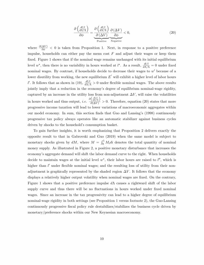
where ∂(∆V )∂φ < 0 is taken from Proposition 1. Next, in response to a positive preference

impulse, households can either pay the menu cost F and adjust their wages or keep them

fixed. Figure 1 shows that if the nominal wage remains unchanged with its initial equilibrium

level w∗, then there is no variability in hours worked at l∗. As a result, dl/ldΛ/Λ = 0 under fixed

nominal wages. By contrast, if households decide to decrease their wages to w′ because of a

lower disutility from working, the new equilibrium E′will exhibit a higher level of labor hours

l′. It follows that as shown in (19), dl/ldΛ/Λ > 0 under flexible nominal wages. The above results

jointly imply that a reduction in the economy’s degree of equilibrium nominal-wage rigidity,

captured by an increase in the utility loss from non-adjustment ∆V , will raise the volatilities

in hours worked and thus output, i.e.∂(dl/ldΛ/Λ

)∂(∆V ) > 0. Therefore, equation (20) states that more

progressive income taxation will lead to lower variations of macroeconomic aggregates within

our model economy. In sum, this section finds that Guo and Lansing’s (1998) continuously

progressive tax policy always operates like an automatic stabilizer against business cycles

driven by shocks to the household’s consumption basket.

To gain further insights, it is worth emphasizing that Proposition 2 delivers exactly the

opposite result to that in Gabrovski and Guo (2019) when the same model is subject to

monetary shocks given by dM , where M =∫ 1

0 Midi denotes the total quantity of nominal

money supply. As illustrated in Figure 2, a positive monetary disturbance that increases the

economy’s aggregate demand will shift the labor demand curve to the right. When households

decide to maintain wages at the initial level w∗, their labor hours are raised to l′′, which is

higher than l′ under flexible nominal wages; and the resulting loss of utility from their non-

adjustment is graphically represented by the shaded region ∆V . It follows that the economy

displays a relatively higher output volatility when nominal wages are fixed. On the contrary,

Figure 1 shows that a positive preference impulse dΛ causes a rightward shift of the labor

supply curve and thus there will be no fluctuations in hours worked under fixed nominal

wages. Since an increase in the tax progressivity can lead to a higher degree of equilibrium

nominal-wage rigidity in both settings (see Proposition 1 versus footnote 2), the Guo-Lansing

continuously progressive fiscal policy rule destabilizes/stabilizes the business cycle driven by

monetary/preference shocks within our New Keynesian macroeconomy.

10

3 Linearly Progressive Taxation

In this section, we adopt Dromel and Pintus’(2007) piece-wise linearly progressive tax formula-

tion to analytically examine its business-cycle stabilization effects within the New Keynesian

macroeconomy described in section 2. The budget constraint faced by the representative

household is modified to∫ 1

0pjcijdj = wili − τ(wili − E)︸ ︷︷ ︸

= TBi

+

∫ 1

0πijdj + Si, 0 < E < α (1− µ) , (21)

where E represents the exemption level of income which is postulated to be strictly positive

such that it is consistent with the actual data of U.S. and many developed countries. The

government will then impose a positive tax rate τ ∈ (0, 1) on the fraction of agent i’s wage

income wili that is higher than this pre-specified threshold E; whereas there is no income

taxation τ = 0 when wili ≤ E. This parsimonious two-income-bracket specification is able

to qualitatively capture the piece-wise linear feature commonly observed in real-world tax

systems, and TBi denotes the associated tax burden or payment for household i. Moreover, the

tax schedule under consideration is said to be “progressive”when wili > E, since the resulting

average tax rate ATRi = τ(1− Ewili

) is lower than the positive and constant marginal tax rate

MTRi = τ . As in Gabrovski and Guo (2019) and the previous section, our analyses below are

restricted to the economy’s symmetric equilibrium under a progressive fiscal policy rule. This

in turn will yield an upper bound on the critical value of income given by E < α (1− µ).5

Given the postulated progressive taxation with wili > E > 0 and 0 < τ < 1, we also follow

Dromel and Pintus (2007) to define the degree of tax progressivity on household i as

θi ≡MTRi −ATRi

1−ATRi=

τE

(1− τ)wili + τE∈ (0, 1), where

∂θi∂τ

> 0 and∂θi∂E

> 0, (22)

i.e. an increase in either the marginal tax rate τ or the threshold income level E will lead

to a more progressive tax scheme. In addition, we will maintain the assumption that each

household’s economic decisions are governed by the common marginal tax rate τ .

Per the same solution procedure of section 2, we find that under linearly progressive income

taxation, the equilibrium conditions that characterize the aggregate demand and market price

for consumption good j, as in equations (6) and (10), will remain the same; and the indirect

utility function for household i now becomes

5Using equations (6), (8), (10), and (26) that will be derived later, together with the goods-market clearingcondition cj = yj , it can be shown that each agent’s nominal wage income at the model’s symmetric equilibriumis given by wl = α (1− µ), which is invariant with respect to preference shocks. It follows that the tax policywill become progressive when α (1− µ) > E > 0.

11

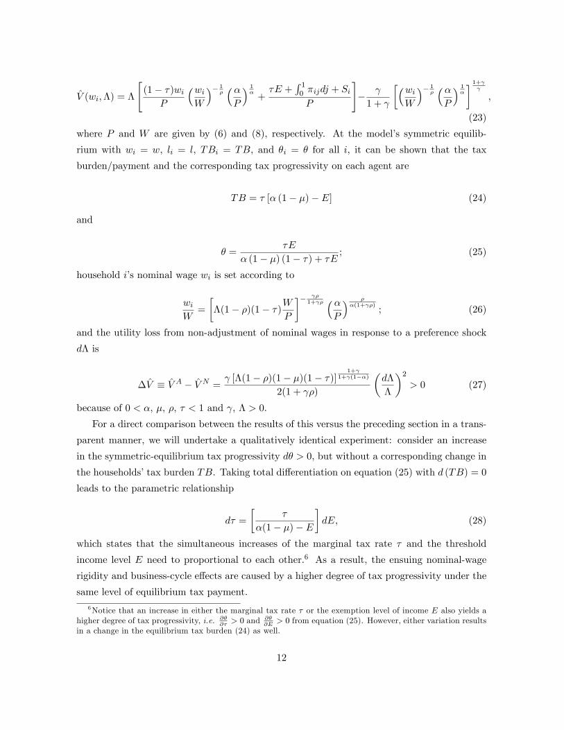
V (wi,Λ) = Λ

[(1− τ)wi

P

(wiW

)− 1ρ(αP

) 1α

+τE +

∫ 10 πijdj + Si

P

]− γ

1 + γ

[(wiW

)− 1ρ(αP

) 1α

] 1+γγ

,

(23)

where P and W are given by (6) and (8), respectively. At the model’s symmetric equilib-

rium with wi = w, li = l, TBi = TB, and θi = θ for all i, it can be shown that the tax

burden/payment and the corresponding tax progressivity on each agent are

TB = τ [α (1− µ)− E] (24)

and

θ =τE

α (1− µ) (1− τ) + τE; (25)

household i’s nominal wage wi is set according to

wiW

=

[Λ(1− ρ)(1− τ)

W

P

]− γρ1+γρ (α

P

) ρα(1+γρ)

; (26)

and the utility loss from non-adjustment of nominal wages in response to a preference shock

dΛ is

∆V ≡ V A − V N =γ [Λ(1− ρ)(1− µ)(1− τ)]

1+γ1+γ(1−α)

2(1 + γρ)

(dΛ

Λ

)2

> 0 (27)

because of 0 < α, µ, ρ, τ < 1 and γ, Λ > 0.

For a direct comparison between the results of this versus the preceding section in a trans-

parent manner, we will undertake a qualitatively identical experiment: consider an increase

in the symmetric-equilibrium tax progressivity dθ > 0, but without a corresponding change in

the households’tax burden TB. Taking total differentiation on equation (25) with d (TB) = 0

leads to the parametric relationship

dτ =

[τ

α(1− µ)− E

]dE, (28)

which states that the simultaneous increases of the marginal tax rate τ and the threshold

income level E need to proportional to each other.6 As a result, the ensuing nominal-wage

rigidity and business-cycle effects are caused by a higher degree of tax progressivity under the

same level of equilibrium tax payment.

6Notice that an increase in either the marginal tax rate τ or the exemption level of income E also yields ahigher degree of tax progressivity, i.e. ∂θ

∂τ> 0 and ∂θ

∂E> 0 from equation (25). However, either variation results

in a change in the equilibrium tax burden (24) as well.

12

Next, we substitute the restriction (28) into the totally differentiated version of (25) to

obtain

dθ|d(TB) = 0 =

[α(1− µ)θ

τE

]dτ, (29)

which yields the size of the tax-progressivity increment, while keeping the associated tax

burden unchanged at its initial equilibrium level. Using equations (27) and (29), together

with the chain rule, it is then straightforward to show that

d(∆V )

dθ

∣∣∣∣∣d(TB) = 0

= −(

∆V

1− τ

)[1 + γ

1 + γ(1− α)

]︸ ︷︷ ︸

=d(∆V )dτ

[τE

α(1− µ)θ

]︸ ︷︷ ︸

= dτdθ

< 0 (30)

because of 0 < α, µ, τ , θ < 1 and γ, E, ∆V > 0. As in the previous section, since a smaller loss

of utility from non-adjustment ∆V enlarges the parametric space that exhibits nominal-wage

rigidity, equation (30) shows that an increase in the degree of tax progressivity θ will enhance

the likelihood of fixed nominal wages in equilibrium. It follows that

Proposition 3. Under a preference shock dΛ and (piece-wise) linearly progressive income

taxation with wili > E > 0 in equilibrium, an increase in the tax progressivity θ ∈ (0,

1) without a corresponding change in the households’ tax burden will always (i) raise the

degree of equilibrium nominal-wage rigidity, and (ii) operate like an automatic stabilizer that

generates lower volatilities in labor hours and output.

The intuition for this Proposition turns out to be qualitatively the same as that underlying

Propositions 1 and 2. Per the earlier discussions associated with Figure 1, consider the econ-

omy’s labor market under a given degree of tax progressivity θ1 that is derived from a marginal

tax rate τ1 ∈ (0, 1) and an exemption level of income E1 > 0. Upon a positive preference shock

that shifts the labor supply curve to the right, it can be shown that agents’nominal income

will remain unchanged with w∗l∗ = w′l′(see footnote 5), regardless of whether their nominal

wages are adjusted or not. This result, together with a reduction in the aggregate price index

as shown in (17), leads to an increase in the before-tax real labor income for “adjusting”house-

holds. It follows that these agents’after-marginal-tax real income (1− τ) wlP may rise or fall

when the tax progressivity is raised to θ2 under higher levels of the marginal tax rate τ2 and

the income threshold E2. Equation (30) analytically shows that since the impact of a higher

gross real labor income is outweighed by the opposing effect of an increase in the marginal

tax rate, more progressive taxation will always decrease the utility loss from non-adjustment

of nominal wages, i.e. d(∆V )dθ < 0 while keeping d (TB) = 0. This in turn implies that each

household is less capable of paying the adjustment cost F needed for changing its nominal

13

wage because of a lower disposable income. Hence, agents are more likely to maintain their

initial nominal wages in response to a preference disturbance as the tax progressivity rises.

Next, it is straightforward to show that an increase in the degree of tax progressivity θ

will reduce the magnitude of business cycle fluctuations. Figure 1 depicts that when agents

decide not to change their nominal wages upon a positive utility impulse, the equilibrium

labor hours remain unaffected(dl/ldΛ/Λ = 0

); and that when the nominal wage is adjusted to

fall, the household also raises its labor supply(dl/ldΛ/Λ > 0

)and produce more consumption

goods. Based on the preceding paragraph which illustrates that fixed nominal wages are more

likely to take place under a higher tax progressivity, the economy will exhibit lower volatilities

in hours worked and total output as a consequence. In sum, our analysis finds that a more

(piece-wise) linearly progressive tax system always raises the equilibrium degree of nominal-

wage rigidity and operates like an automatic stabilizer against cyclical fluctuations driven by

preference shocks.

To summarize, this paper has overturned the business-cycle destabilization result of more

progressive income taxation à la Gabrovski and Guo (2019) within the same New Keyne-

sian model driven by impulses to the household utility (cf. the quantity of nominal money

supply). Under the Guo-Lansing continuously or the Dromel-Pintus linearly progressive tax

schedule with the equilibrium tax burden unchanged, we analytically show that an increase

in the (positive) tax progressivity will always enhance the likelihood of fixed nominal wages

in equilibrium and mitigate macroeconomic fluctuations caused by preference shocks. The

key insight is that although both preference and monetary disturbances affect the economy’s

aggregate demand, they will generate very different effects in the labor market: a preference

shock shifts the household’s labor supply curve (see Figure 1), whereas a monetary shock shifts

the firm’s labor demand curve (see Figure 2). As a result, our analysis concludes that whether

a more progressive fiscal policy rule (de)stabilizes the Kleven-Kreiner macroeconomy depends

crucially on the driving source of business cycles.7

7For the sake of theoretical completeness, we have also studied our model economy with flat income taxationwhereby the average and marginal tax rates for all households take on the same constant level given by (i)ti = tmi = η ∈ (0, 1) under the Guo-Lansing continuously progressive tax schedule; or (ii) E = 0 and ATRi =MTRi = τ ∈ (0, 1) under the Dromel-Pintus linearly progressive policy rule. In this case, the tax-progressivity

parameter φ or θ is equal to zero. Moreover, it is straightforward to obtain ∂(∆V )∂η

< 0 and ∂(∆V )∂τ

< 0, indicatingthat a higher tax rate will make agents more willing to keep their nominal wages unchanged in response to apreference shock. This result, together with our earlier discussions on the labor market as shown in Figure 1,implies that a flat tax policy will always stabilize the Kleven-Kreiner macroeconomy with lower volatilities ofhours worked and total output driven by utility disturbances.

14

4 Conclusion

In our previous work, Gabrovski and Guo (2019) find that more progressive income taxation

may operate like an automatic destabilizer which generates higher cyclical volatilities of la-

bor hours and total output within a prototypical New Keynesian macroeconomy driven by

shocks to aggregate money supply. The current paper demonstrates that this business-cycle

destabilization result is not robust to a slight departure whereby the same analytical frame-

work is subject to impulses to the household’s marginal utility of consumption. Under either

Guo and Lansing’s (1998) continuously progressive fiscal policy rule, or Dromel and Pintus’

(2007) piece-wise linearly progressive tax scheme, we analytically show that an increase in the

(positive) tax progressivity without a corresponding change in the household’s tax burden will

always raise the economy’s equilibrium degree of nominal-wage rigidity upon a positive pref-

erence shock, and thus serve as an automatic stabilizer to alleviate the resulting magnitude

of cyclical fluctuations. From a policy standpoint, the findings of our two articles altogether

illustrate that in the context of Kleven and Kreiner’s (2003) model with imperfect competition

and sticky nominal wages, whether a more progressive tax schedule (de)stabilizes the busi-

ness cycle depends crucially on the driving source which leads to variations in macroeconomic

aggregates.

Our analyses can be extended in several directions. For example, it would be worth-

while to extend our model economy to an intertemporal setting with capital accumulation

dynamics. In addition, we may incorporate features that are commonly adopted in the New-

Keynesian literature, such as nominal price rigidities and investment adjustment costs, among

others. These possible extensions will allow us to examine the robustness of this paper’s the-

oretical results and policy implications, as well as further enhance our understanding of the

business-cycle (de)stabilization effects of progressive income taxation within a New-Keynesian

macroeconomy. We plan to pursue these research projects in the near future.

5 Conflict of Interest Statement

The authors declare that they have no conflict of interest that could have appeared to

influence the work reported in this paper.

Miroslav Gabrovski and Jang-Ting Guo, 3/1/2021.

15

References[1] Bencivenga, V.R. (1992), “An Econometric Study of Hours and Output Variation with

Preference Shocks,”International Economic Review 33, 449-471.

[2] Dromel, N.L. and P.A. Pintus (2007), “Linearly Progressive Income Taxes and Stabiliza-tion,”Research in Economics 61, 25-29.

[3] Gabrovski, M. and J.-T. Guo (2019), “A Note on Progressive Taxation, Nominal WageRigidity, and Business Cycle Destabilization,”forthcoming in Macroeconomic Dynamics.

[4] Guo, J.-T. and K.J. Lansing (1998), “Indeterminacy and Stabilization Policy,”Journal ofEconomic Theory 82, 481-490.

[5] Kleven, H.J. and C.T. Kreiner (2003), “The Role of Taxes as Automatic Destabilizers inNew Keynesian Economics,”Journal of Public Economics 87, 1123-1136.

[6] Mattesini, F. and Rossi, L. (2012), “Monetary Policy and Automatic Stabilizers: The Roleof Progressive Taxation,”Journal of Money, Credit and Banking 44, 825-862.

[7] Schmitt-Grohé, S. and M. Uribe (1997), “Balanced-Budget Rules, Distortionary Taxes andAggregate Instability,”Journal of Political Economy 105, 976-1000.

16

Figure 1: Labor Market under a Positive Preference Shock

Figure 2: Labor Market under a Positive Monetary Shock