Project01 — Fys4460 — 2018 3

Project01 — Fys4460 — 2018

Project 1: Introductory Molecular Dynamics ModelingThrough this project you will learn to use molecular dynamics to addressthe behavior of single atoms and molecules with particular emphasis onunderstanding the statistical properties of he system.

Atomic modeling basics. How do we determine the motion of a systemof atoms? Here, we will use a classical approximation to describe themotion of a system of atoms. In this approximation, we use Newton’slaws of motion and a well-chosen description of the forces between atomsto find the motion of the atoms. The forces are described by the potentialenergies of the atoms given their positions. The potential energy functionscan, in principle, be determined from quantum mechanical calculationsbecause the forces and the potential energies depend on the states ofthe electrons — it is the electrons that form the bonds between atomsand are the origin of the forces between atoms. However, in the classicalapproximation we parametrize this problem: We construct simplifiedmodels for the interactions that provide the most important features ofthe interactions.

Interatomic potentials. The behavior of a system will depend on thepotential energy and how it depends on the positions of all the particles.In general, we assume that the potential energy, U , depends on thepositions, ri, of all the particles:

U = U ({ri}) . (0.1)

This is a simplification. In general, the potential energy may dependon additional internal states of the interactions between the atoms. Forexample, we may know that two atoms interact through a covalentbond, and may therefore prescribe this covalent bond as part of thepotential energy: The energy would depend both on the positions of theparticles and on what particles are connected by these covalent bonds.Here, we will consider two types of interactions: bonded interactionswhere the interaction types between atoms are prescribed and does notchange throughout the simulation, and non-bonded interactions, wherethe potential energy only depends on the positions of the particles. Non-bonded interactions open for modeling more complicated interactionsbetween atoms, including the formation and breaking of strong bondsbetween atoms.

4 Project01 — Fys4460 — 2018

We will start by assuming that the potential energy can be writtenas a sequence of interactions of higher and higher order, starting frompair-wise interactions, then moving on two three-particle-interactions,four-particle-interactions and so on. We can then write the potentialenergy as

U ({ri}) =ÿ

ij

Uij (ri, rj) +ÿ

ijk

Uijk (ri, rj , rk) + . . . . (0.2)

Here, we will first address a model that only includes two-particle-interactions, then move on to address a model with three-particle-interactions, and finally address several models for the interactionsbetween water molecules.

Lennard-Jones potential. One of the simplest models for atom-atominteractions is a representation of the interactions between nobel-gasatoms, such as between two Argon atoms. For the interaction betweentwo noble-gas atoms we have two main contributions:

• There is an attractive force due to a dipole-dipole interaction. Thepotential for this interactions is proportional to (1/r)6, where r isthe distance between the atoms. This interaction is called the vander Waals interaction and we call the corresponding force the van derWaals force.

• There is a repulsive force which is a quantum mechanical e�ect due tothe possibility of overlapping electron orbitals as the two atoms arepushed together. We use a power-law of the form (1/r)n to representthis interaction. It is common to choose n = 12, which gives a goodapproximation for the behavior of Argon.

The combined model is called the Lennard-Jones potential:

U(r) = 4‘

A3‡

r

412≠

3‡

r

46B

. (0.3)

Here, ‘ is a characteristic energy, which is specific for the atoms weare modeling, and ‡ is a characteristic length.

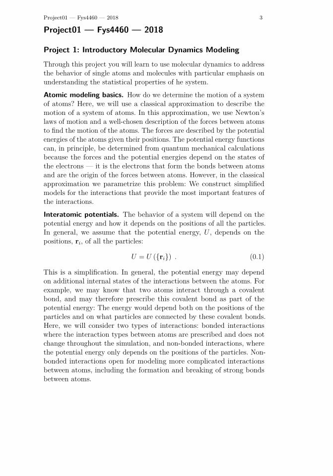
The Lennard-Jones potential and the corresponding force F (r) isillustrated in Fig. 0.1. We see that the Lennard-Jones potential reaches

Project01 — Fys4460 — 2018 5

Fig. 0.1 Illustration of the

Lennard-Jones potential.

r=<0.8 1 1.2 1.4 1.6 1.8 2 2.2 2.4

U=0

0

-6

-4

-2

0

2

4

6

its minimum whenF (r) = ≠ d

drU(r) = 0 , (0.4)

which occurs at

F (r) = 24 ‘01(‡/r)6 ≠ 2 (‡/r)12

2= 0 ∆ r

‡= 21/6 . (0.5)

We will use this potential to model the behavior of an Argon system.However, the Lennard-Jones potential is often used not only as a modelfor a noble gas, but as a fundamental model that reproduces behavior thatis representative for systems with many particles. Indeed, Lennard-Jonesmodels are often used as base building blocks in many interatomic poten-tials, such as for the interaction between water molecules and methaneand many other systems where the interactions between molecules orbetween molecules and atoms is simplified (coarse grained) into a single,simple potential. Using the Lennard-Jones model you can model 102 to106 atoms on your laptop and we can model 1010-1011 atoms on largesupercomputers.

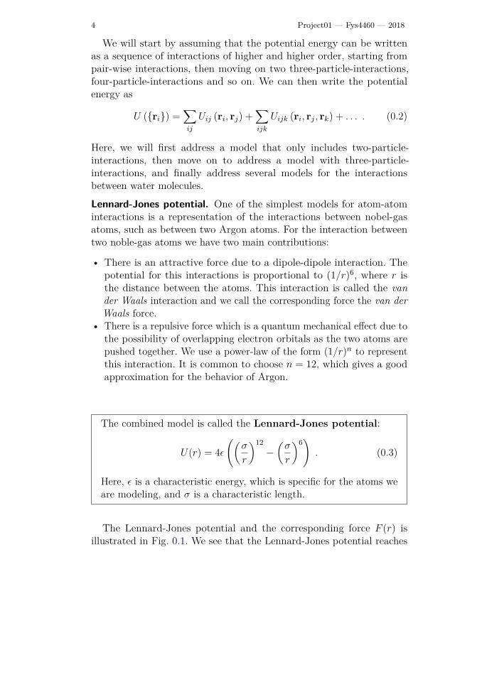
Initial conditions. An atomic (molecular) dynamics simulation startsfrom an initial configuration of atoms and determines the trajectoriesof all the atoms. The initial condition for such a simulation consists ofall the positions, ri(t0) and velocities vi(t0) at the initial time t0. Inorder to model a realistic system, it is important to choose the initialconfiguration with some care. In particular, since most potentials suchas the Lennard-Jones potential increase very rapidly as the interatomicdistance r goes to zero, it is important not to place the atoms too closeto each other. We therefore often place the atoms regularly in space, ona lattice, with initial random velocities.

We generate a lattice by first constructing a unit cell and then copyingthis unit cell to each position of a lattice to form a regular pattern ofunit cells. (The unit cell may contain more than one atom). Here, we willuse cubic unit cells. For a cubic unit cell of length b with only one atom

6 Project01 — Fys4460 — 2018

Fig. 0.2 a Illustration of a

unit cell for a square lattice.

b A system consisting of

4 ◊ 4 unit cells, where each

of the cells are marked and

indexed for illustration.

b

b

b

b

L=4 b

L=4

b

(a) (b)

cell(1,1) cell(2,1) cell(3,1) cell(4,1)

cell(1,2) cell(2,2) cell(3,2) cell(4,2)

cell(1,3) cell(2,3) cell(3,3) cell(4,3)

cell(1,4) cell(2,4) cell(3,4) cell(4,4)

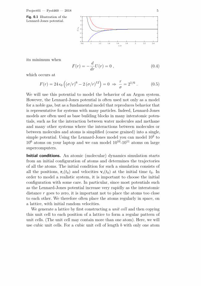
Fig. 0.3 Left Illustration

of a unit cell for a face

centered cubic lattice. Unit

cell atoms illustrated in

blue and the base position

of other cells shown in red.

Right A system consisting

of 10 ◊ 10 ◊ 10 unit cells.

in each unit cell, we can place the atom at (0, 0, 0) in the unit cell andgenerate a cubic lattice with distances b between the atoms by using thiscubic unit cell to build a lattice. This is illustrated for a two-dimensionalsystem in Fig. 0.2. Such a lattice is called a simple cubic lattice.

However, for a Lennard-Jones system we know (from other theoretical,numerical and experimental studies) that the equilibrium crystal structureis not a simple cubic lattice, but a face centered cubic lattice. This isa cubic lattice, with additional atoms added on the center of each ofthe faces of the cubes. The unit cell for a face centered cubic lattice isillustrated in Fig. 0.3. We will use this as our basis for a simulation andthen select a lattice size b so that we get a given density of atoms. Thewhole system will then consist of L ◊ L ◊ L cells, each of size b ◊ b ◊ band with 4 atoms in each cell.Boundary conditions. A typical molecular model of a liquid of Argonmolecules is illustrated in Fig. 0.4a. In this case, we have illustrateda small system of approximately 10 ◊ 10 ◊ 10 atom diameters in size.Below, you will learn how to set up and simulate such systems on yourlaptop. Unfortunately, you will not be able to model macroscopicallylarge systems — neither on your laptop nor on the largest machine in theworld. A liter of gas at room temperature typically contains about 1023

atoms, and this is simply beyond practical computational capabilities.But it is possible with a small system to gain some insights into how

very large, even infinite, systems behave? One of the problems with the10 ◊ 10 ◊ 10 system above is the external boundaries. But we can fool

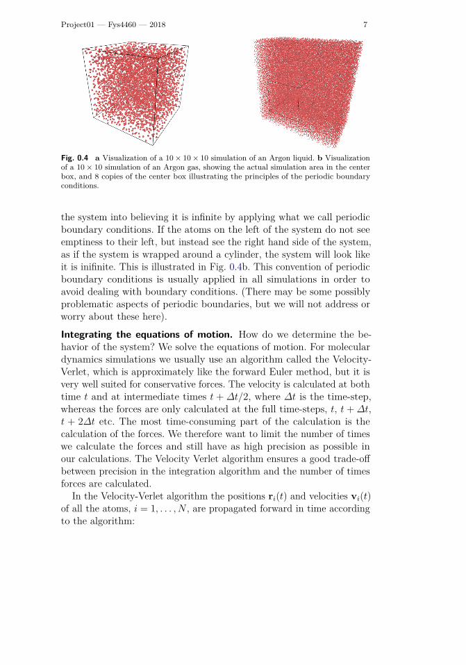
Project01 — Fys4460 — 2018 7

Fig. 0.4 a Visualization of a 10 ◊ 10 ◊ 10 simulation of an Argon liquid. b Visualization

of a 10 ◊ 10 simulation of an Argon gas, showing the actual simulation area in the center

box, and 8 copies of the center box illustrating the principles of the periodic boundary

conditions.

the system into believing it is infinite by applying what we call periodicboundary conditions. If the atoms on the left of the system do not seeemptiness to their left, but instead see the right hand side of the system,as if the system is wrapped around a cylinder, the system will look likeit is inifinite. This is illustrated in Fig. 0.4b. This convention of periodicboundary conditions is usually applied in all simulations in order toavoid dealing with boundary conditions. (There may be some possiblyproblematic aspects of periodic boundaries, but we will not address orworry about these here).

Integrating the equations of motion. How do we determine the be-havior of the system? We solve the equations of motion. For moleculardynamics simulations we usually use an algorithm called the Velocity-Verlet, which is approximately like the forward Euler method, but it isvery well suited for conservative forces. The velocity is calculated at bothtime t and at intermediate times t + ∆t/2, where ∆t is the time-step,whereas the forces are only calculated at the full time-steps, t, t + ∆t,t + 2∆t etc. The most time-consuming part of the calculation is thecalculation of the forces. We therefore want to limit the number of timeswe calculate the forces and still have as high precision as possible inour calculations. The Velocity Verlet algorithm ensures a good trade-o�between precision in the integration algorithm and the number of timesforces are calculated.

In the Velocity-Verlet algorithm the positions ri(t) and velocities vi(t)of all the atoms, i = 1, . . . , N , are propagated forward in time accordingto the algorithm:

8 Project01 — Fys4460 — 2018

vi(t + ∆t/2) = v(t) + Fi(t)/mi∆t/2 (0.6)ri(t + ∆t) = r(t) + vi(t + ∆t/2) (0.7)Fi(t + ∆t) = ≠ÒV (ri(t + ∆t)) (0.8)vi(t + ∆t) = v(t + ∆t/2) + Fi(t + ∆t)/mi∆t/2 , , (0.9)

This method has very good properties when it comes to energy conserva-tion, and it does, of course, preserve momentum perfectly.Non-dimensional equations of motion. However, all the quantities ina molecular dynamics simulations are very small. It is therefore usualto introduce measurement units that are adapted to the task. For theLennard-Jones model we usually use the intrinsic length and energy scaleof the model as the basic units of length and energy. This means that wemeasure lengths in units of ‡ and energies in units of ‘0. A vector r

Õi

inthe simulation is therefore related to the real-world length ri through

ri = ‡ rÕi

… rÕi

= ri/‡ . (0.10)

Similarly, we can introduce a Lennard-Jones time, · = ‡

m/‘, where mis the mass of the atoms, and the Lennard-Jones temperature T0 = ‘/kB .Using these notations, we can rewrite the equations of motion for theLennard-Jones system using the non-dimensional position and time,r

Õi

= ri/‡ and tÕ = t/· :

md2

dt2 ri =ÿ

j

24‘01(‡/rij)6 ≠ 2 (‡/rij)12

2 1rij/r2

ij

2, (0.11)

to become

d2

d(tÕ)2 rÕi

=ÿ

j

241r≠6

ij≠ 2r≠12

ij

2 1r

Õij

/rÕ2ij

2. (0.12)

Notice that this equation is general. All the specifics of the system isnow part of the characteristic length, time and energy scales ‡, · , and ‘0.For Argon ‡ = 0.3405µm, and ‘ = 1.0318 · 10≠2eV, and for other atomsyou need to find the corresponding parameter values.

Quantity Equation Conversion factor Value for Argon

Length xÕ= x/L0 L0 = ‡ 0.3405µm

Time tÕ= t/tau · = ‡

m/‘ 2.1569 · 10

3fs

Force F Õ= F/F0 F0 = m‡/·2

= ‘/‡ 3.0303 · 10≠1

Energy EÕ= E/E0 E0 = ‘ 1.0318 · 10

≠2eV

Temperature T Õ= T/T0 T0 = ‘/kB 119.74 K

Project01 — Fys4460 — 2018 9

Running a molecular dynamics simulation. There are several e�cientpackages that solves the equations of motion for a molecular dynamicssimulation. The packages allow us to model a wide variety of systems,atoms and molecules, and are e�cienty implemented on various comput-ing platforms, making use of modern hardware on your laptop or desktopor state-of-the-art supercomputing fascilities. We use a particular tooldeveloped at Sandia National Laboratories called LAMMPS.Installation of LAMMPS. If you want to be able to reproduce thesimulations performed here you will need to install LAMMPS on yourcomputer. This is very simple if you have a Mac or an Ubuntu system —for a windows system you will have to follow the installation instructionsfound at the web-site for LAMMPS. You can find all the documentationof LAMMS here.Mac installation. On a mac you should be able to install LAMMS usingHomebrew or Macports.

Using Homebrew (Homebrew) LAMMPS is installed with:

brew tap homebrew/sciencebrew install lammps

If you want to use the parallell implementation of LAMMPS you caninstall this version using

brew tap homebrew/sciencebrew install lammps --with-mpi

Using MacPorts (MacPorts) LAMMPS is installed with:

port install lammps

Ubuntu installation. You can install a recent version of LAMMPSwith:

sudo apt-get install lammps

Starting a simluation in LAMMPS. If you have successfully installedLAMMPS, you are ready to start your first molecular dynamics simula-tions. The LAMMPS simulator reads its instructions on how to run asimulation from an input file with a specific syntax. Here, we will set upa three-dimensional simulation of a Lennard-Jones system using the filein.myfirstmd:

10 Project01 — Fys4460 — 2018

# 3d Lennard-Jones gasunits ljdimension 3boundary p p patom_style atomic

lattice fcc 0.01region simbox block 0 10 0 10 0 10create_box 1 simboxcreate_atoms 1 box

mass 1 1.0velocity all create 2.5 87287

pair_style lj/cut 3.0pair_coeff 1 1 1.0 1.0 3.0

fix 1 all nve

dump 1 all custom 10 dump.lammpstrj id type x y z vx vy vzthermo 100run 5000

The simulation is run from the command line in a Terminal. Notice thatthe file in.myfirstmd must be in your current directory. I suggest creat-ing a new directory for each simulation, copying the file in.myfirstmdinto the directory and modifying the file to set up your simulation, beforestarting the simulation with:

lammps < in.myfirstmd

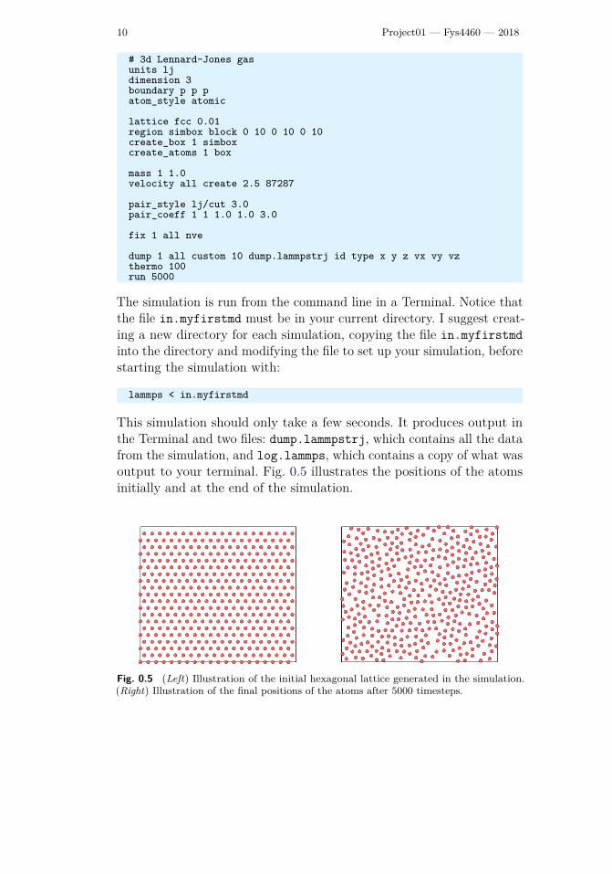
This simulation should only take a few seconds. It produces output inthe Terminal and two files: dump.lammpstrj, which contains all the datafrom the simulation, and log.lammps, which contains a copy of what wasoutput to your terminal. Fig. 0.5 illustrates the positions of the atomsinitially and at the end of the simulation.

Fig. 0.5 (Left) Illustration of the initial hexagonal lattice generated in the simulation.

(Right) Illustration of the final positions of the atoms after 5000 timesteps.

Project01 — Fys4460 — 2018 11

The input file in.myfirstmd consists of a series of commands to beinterpreted by LAMMPS. Here, we look at what these do in detail.(You can skip this at first reading, and return when you wonderwhat the parameters actually do).

# 3d Lennard-Jones gas

This line starts with a # and is a comment that is ignored by theprogram.

units ljdimension 3boundary p p patom_style atomic

This block describes general features of the simulation:The units lj command selects Lennard-Jones units, which were

introduced above. This means that lengths are measured in unitsof ‡, energies in units of ‘0, time in units of · = ‡

m/‘, and

temperature in terms of T0 = ‘/kB. For Argon ‡ = 0.3405µm, and‘ = 1.0318 ·10≠2eV. Other atomic models will have other parameters.

The dimension command specifies the dimensionality of the sim-ulation: 2 or 3. Here we run a 3d simulation.

The boundary command specifies boundary conditions to be ap-plied. Here we have periodic boundaries in the x-, y-, and z- direc-tions.

The atom_style command specifies the complexity of the descrip-tion of each atom/particle. Here, we will use the simplest description,atomic, which is used for noble gases and coarse-grained simulationmodels.

lattice fcc 0.01region simbox block 0 10 0 10 0 10create_box 1 simboxcreate_atoms 1 box

This block sets up the dimensions of the 10 ◊ 10 ◊ 10 simulationbox and fills the box with atoms with a given packing fraction.

The lattice command generates a lattice of points. This does,surprisingly enough, not actually generate any atoms, it only gener-ates a set of positions in space where atoms will be generated whenwe generate atoms. The type fcc specifies a three-dimensional latticeof face-centered-cubic shape. And the number 0.01 is called the

12 Project01 — Fys4460 — 2018

scale and is the reduced density, flÕ, when we have chosen LJ unitsfor the simulation. (Notice that the scale is interpreted di�erently ifwe do not use LJ units, see the LAMMPS documentation for moreinformation).

The region command defines a region which is a block extendingover 0 < x < 10, 0 < y < 10, 0 < z < 10 We give this region thename simbox.

The create_box command now actually creates the simulationbox based on the spatial region we called simbox. The simulationbox will only contain 1 (one) type of atoms, hence the number 1.

The create_atoms finally fills the simulation box we have definedusing the lattice we have defined with atoms of type 1.

mass 1 1.0velocity all create 2.5 87287

This block defines the material properties of the atoms and definestheir initial velocities.

The mass command defines that atoms of type 1 will have a massof 1.0 relative to the mass of the Lennard-Jones model. This meansthat all atoms have mass 1 in the Lennard-Jones units. This meansthat the masses of all the atoms are the same as the mass m used inthe non-dimensionalization of the Lennard-Jones model.

The velocity command generates random velocities (using aGaussian distribution) so that the initial temperature for all atomtypes in the system is 2.5 in the dimensionless Lennard-Jones units.The last, strange integer number 87287 is the seed for the randomnumber generator used to generate the random numbers. As long asyou do not change the seed number you will always generate sameinitial distribution of velocities for this simulation.

pair_style lj/cut 3.0pair_coeff 1 1 1.0 1.0 3.0

This block specifies the potential between the atoms.The pair_style command specifies the we want to use a Lennard-

Jones potential with a cut-o� that is of length 3.0. What does thismean? It means that since the Lennard-Jones potential falls soquickly to zero as the distance between the atoms increase, we willapproximate interaction to be zero when the atoms are further than3.0 away from each other (measured in Lennard-Jones units, that is

Project01 — Fys4460 — 2018 13

in units of ‡). The simulator ensures that both the potential and theforce is continuous across the transition. There are many other typesof force fields that you may use — take a look at the documentationof LAMMPS for ideas and examples.

The pair_coeff command specifies the parameters of theLennard-Jones model. The two first numbers, 1 1, specifies that wedescribe the interaction of atoms of type 1 with atoms of type 1.And the parameters of the Lennard-Jones model are 1.0 1.0 3.0.This means that The interaction between an atom of type 1 with anatom of type 1 has a ‡-value corresponding 1.0 times the the general‡-value (hence the first number 1.0), and a ‘0-value correspondingto 1.0 times the overall ‘-value (hence the second number 1.0). Thecut-o� for this interaction is 3.0 — the same value as we specifiedabove.

fix 1 all nve

This one-line block specifies what type of simulation we are per-forming on the atoms. This is done by one or more fix commandsthat can be applied to regions of atoms. Here, the fix, which wecall 1 (you can choose numbers or names for identity), is appliedto all particles and specifies that the simulation is run at constantnve, that is, at constant number of particles (n), constant volume(v, meaning that the simulation box does not change during thesimulation), and constant energy (e). You may be surprised by theconstant energy part. Does the integration algorithm ensure thatthe energy is constant. Yes, it does. However, there can be caseswhere we want to add energy to a particular part of the system, andin that case the basic interation algorithm still conserves energy, butwe add additional terms that may change the total energy of thesystem.

dump 1 all custom 10 dump.lammpstrj id type x y z vx vy vzthermo 100run 5000

This block specifies simulation control, inclusing output and thenumber of time-steps to simulate.

The dump command tells the simulator to output the state. The1 is the name we give this dump — it could also have been given aname such as mydump. We specify that all atoms are to be output

14 Project01 — Fys4460 — 2018

using a custom output format, with output every 10 time-stepsto the file dump.lammpstrj, and the ‘id type x y z vx vy vz’ listspecifies what is output per atom.

The thermo command specifies that output to the Terminal andto the log file, log.lammps, is provided every 100 timesteps.

The run command starts the simulation and specifies that it willrun for 5000 timesteps.

Visualizing the results of a simulation. It is good practice to look atthe results of the simulation. Use for example Ovito to visualize theresults.

Macroscopic observables. We can use the MD simulation to measuremacroscopic quantities by averaging properties of the simulation system.The ergodic hypothesis states that the time a system has one particularvalue of an observable A is proportional to the phase space volume whereA has this value. This applies to systems in equilibrium studied for a longperiod of time. As a result, the time average and ensemble average of avariable are equal. If we average over long enough periods of time, andour microscopic interaction model is correct, we can use the models topredict equilibrium properties of real systems. In addition, we can use thesimulation to gain insight into the statistical properties of systems withmany particles, and in particular into the fluctuations in such systems.

a) According to the central limit theorem, the velocity distribution of theparticles will eventually evolve into a Maxwell-Boltzmann distributionindependent of the initial conditions. Let us test this by starting thesimulation with velocities that are uniformly distributed random numbersin the interval [≠v, v], for your own choice of v (You will actually providethe value of T and not v). Look at the description of the ´velocity´command in Lammps to see how to specify a uniform distribution.Investigate the probability density for the velocities and for the speeds ofthe atoms at a given time by writing the velocities to a file and visualizingthe results in a histogram. Study the time-development of the velocitydistribution to estimate how long time it takes for the velocities to reacha Maxwell-Boltzmann distribution. Hint: You can find the histogramhi(t) for a given set of bins of velocities, vi. You can characterize thetime development of hi(t) by looking at the normalized inner product,q

ihi(t)hi(tn)/

qihi(tn)hi(tn), where tn is the final time-step in your

simulation.

Project01 — Fys4460 — 2018 15

We are modelling a micro-canonical ensamble, since we study systemswith constant volume and a constant number of particles, and, in theory,constant energy. In practice, though, our integration scheme does notconserve energy exactly.

b) Find the total energy (kinetic and potential) of the system, E(t), andplot it as a function of time. How does the size of the fluctuations inenergy depend on the time-step ∆t? (Hint: Use the ´timestep´ commandin Lammps to change the timestep in the simulation). Check a few valuesof ∆t to ensure your choice provides reasonable results.

In general, it is not trivial to calculate the temperature for generalpotential forms. The simplest estimate assumes equilibrium betweenthe translational and potential degrees of freedom. According to theequipartition principle, the average total kinetic energy is

ÈEkÍ = 32NkBT (0.13)

where N is the number of atoms and T is our estimate for the systemtemperature.

c) Use this method to measure the temperature as a function of time,T (t). (Don’t forget to equilibriate the system first). Find the averagetemperature of the system (after equilibration), and compare with thetemperature you used to generate the initial velocity distribution. Char-acterize the fluctuations in temperature, and find how the fluctuationsvary with system size.

There are several ways of measuring the pressure P of a many-atomsystem. The method we will use, and which is implemented in Lammps,is derived from the virial equation for the pressure. In a volume V withparticle density fl = N/V , the average pressure is

P = flkBT + 13V

ÿ

i<j

Fij · rij , (0.14)

where the sum runs over all interacting particle pairs. Note that thisexpression depends on the ensemble – and is valid for the micro-canonicalensemble only. The vector products should be computed and summedup inside the force loops for e�ciency.

d) Measure the pressure as a function of temperature in your system, plotP (T ), and discuss the result. How do they compare with your theoreticalexpectations?

16 Project01 — Fys4460 — 2018

e) Measure the pressure as a function of both temperature and density,visualize and discuss the results in comparison with relevant theoreti-cal models. Can you predict the parameters in the model using thesesimulations?

The di�usion constant. We want to characterize transport in a fluid bymeasuring the self-di�usion of an atom: We give an atom i a label, andmeasure its position as a function of time, ri(t). We find the di�usionconstant from the mean square displacement of all atoms (we trace themotion of every atom):

Èr2(t)Í = 1N

Nÿ

i=1(r(t) ≠ rinitial) . (0.15)

From theoretical considerations of the di�usion process we can relatethe di�usion constant in the liquid to the mean squear displacementthrough:

Èr2(t)Í = 6Dt when t æ Œ . (0.16)

This result is similar to the behavior of a random walker in three dimen-sions, which is indeed a good approximation to the motion of an atom ina fluid.

f) Plot the mean square displacement as a function of time and estimatethe di�usion constant, D. Investigate the e�ect of temperature by findingD(t) for some temperatures of your own choice in the liquid phase ofArgon. Remember that you are measuring the total distance travelled bythe atoms, which must be continous when an atom is displaced thoughthe periodic boundaries!

Microscopic structure – radial distribution functions. The radial dis-tribution function g(r), also called a pair correlation function, is a toolfor characterizing the microscopic structure of a fluid. It is interpretedas the radial probability for finding another atom a distance r from anarbitrary atom, or equivalently, the atomic density in a spherical shell ofradius r around an atom. It is commonly normalized by dividing it withthe average particle density so that limræŒ g(r) = 1.

g) Estimate g(r) for r œ (0, L

2 ] in your Argon system. The easiest way isto divide the distance interval into bins, loop over all pairs of particlesand count how many distances belong in each bin. Time-averaging thefunction gives a better description of the system’s general behaviour.Plot g(r) for temperatures where the system is in solid and liquid phases.

Project01 — Fys4460 — 2018 17

Does it appear as expected? How would the exact g(r) look for a perfectcrystal?

Thermostats. In order to simulate the canonical ensemble, interactionswith an external heat bath must be taken into account. Many methodshave been suggested in order to achieve this, all with their pros and cons.Requirements for a good thermostat are:

1. Keeping the system temperature around the heat bath temperature2. Sampling the phase space corresponding to the canonical ensemble3. Tunability4. Preservation of dynamics

The method closest to fullfilling these requirements which is in widespreaduse is the Nosé-Hoover thermostat, which is somewhat complicated toimplement, but is the standard in Lammps.

Some thermostats work by rescaling the velocities of all atoms bymultiplying them with a factor “. The Berendsen thermostat uses

“ =Û

1 + ∆t

·

3Tbath

T≠ 1

4. (0.17)

with · as the relaxation time, tuning the coupling to the heat bath.Though it satisfies Fourier’s law of heat transfer (the transfered heatbetween two bodies is proportional to their temperature di�erence) itdoes a poor job at sampling the canonical ensemble.

h) Discuss possible challenges with the Berendsen thermostat.The Andersen thermostat simulates (hard) collisions between atoms

inside the system and in the heat bath. Atoms which collide will gain anew normally distributed velocity with standard deviation

kBTbath/m.

For all atoms, a random uniformly distributed number in the interval[0, 1] is generated. If this number is less than ∆t

·, the atom is assigned a

new velocity. In this case, · is treated as a collision time, and should haveabout the same value as the · in the Berendsen thermostat. The Andersenthermostat is very useful when equilibrating systems, but disturbs thedynamics of e.g. lattice vibrations.

i) Use the Andersen thermostat, and compare T (t) graphs for simulationsusing the Anderson and he Noose-Hoover thermostats. Be aware that ourT is just an approximation to the real temperature. Describe the impactof the thermostat on the observed dynamics of the system of atoms – asseen in your visualizations of the dynamics.

18 Project01 — Fys4460 — 2018

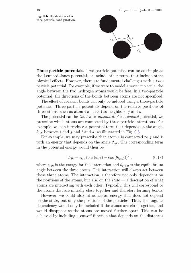
Fig. 0.6 Illustration of a

thee-particle configuration.

i

j

k

θi,j,k

ri,j

ri,k

Three-particle-potentials. Two-particle potential can be as simple asthe Lennard-Jones potential, or include other terms that include otherphysical e�ects. However, there are fundamental challenges with a two-particle potential. For example, if we were to model a water molecule, theangle between the two hydrogen atoms would be free. In a two-particlepotential, the directions of the bonds between atoms are not specificed.

The e�ect of covalent bonds can only be induced using a three-particlepotential. Three-particle potentials depend on the relative positions ofthree atoms, such as atom i and its two neighbors, j and k.

The potential can be bonded or unbonded. For a bonded potential, weprescribe which atoms are connected by three-particle interations. Forexample, we can introduce a potential term that depends on the angle,◊ijk between i and j and i and k, as illustrated in Fig. 0.6

For example, we may prescribe that atom i is connected to j and kwith an energy that depends on the angle ◊ijk. The corresponding termin the potential energy would then be

Vijk = ‘ijk (cos (◊ijk) ≠ cos (◊ijk,0))2 , (0.18)

where ‘ijk is the energy for this interaction and ◊ijk,0 is the equiliubriumangle between the three atoms. This interaction will always act betweenthese three atoms. The interaction is therefore not only dependent onthe positions of the atoms, but also on the state — a description of whatatoms are interacting with each other. Typically, this will correspond tothe atoms that are initially close together and therefore forming bonds.

However, we could also introduce an energy that does not dependon the state, but only the positions of the particles. Thus, the angulardependency would only be included if the atoms are close together, andwould disappear as the atoms are moved further apart. This can beachieved by including a cut-o� function that depends on the distances

Project01 — Fys4460 — 2018 19

rij and rik. Typically, we will introduce a cut-o� for rij and a cut-o� forrik and multiply the two.

An example of a potential with both two-particle and three-particleinteractions is the Stillinger-Weber potential. In general, this potential isdescribed by the following potential energy function:

E =ÿ

i

ÿ

j

V2 (rij) + (0.19)

ÿ

i

ÿ

j

ÿ

k

V3 (rij , rik, ◊ijk) , (0.20)

V2 (rij) = Aij‘ij

C

Bij

A‡ij

rij

Bpij

≠A

‡ij

rij

BqijD

(0.21)

expA

‡ij

rij ≠ aij‡ij

B

, (0.22)

V3 (rij , rik, ◊ijk) = ⁄ijk‘ijk [cos ◊ijk ≠ cos ◊ijk,0]2 (0.23)

expA

“ij‡ij

rij ≠ aij‡ij

B

expA

“ik‡ik

rij ≠ aik‡ik

B

.(0.24)

First, we notice that all the parameters may depend on the type of atom.For a case where all the atoms are the same, we expect all of theseconstants to be the same.

We notice that the two-particle part is similar to the Lennard-Jonesform we studied previously, but with exponents p and q that can bevaried. In addition, a cut-o� function has been introduced. This cut-o�is a function, f(u) of the di�erence u = rij/‡ij ≠ aij :

f(u) = exp (1/u) . (0.25)

Similar cut-o� functions are introduced for the angular dependence.The Stillinger-Weber potential is a good model for silicon, Si, and can

also be a good approximation for structures that involve Si. However, wewould recommend the Vashishta potential for SiC or SiO2.

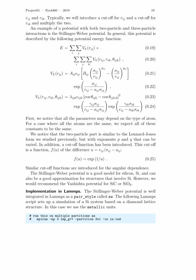
Implementation in Lammps. The Stillinger-Weber potential is wellintegrated in Lammps as a pair_style called sw. The following Lammpsscript sets up a simulation of a Si system based on a diamond latticestructure. In this case we use the metallic units.

# run this on multiple partitions as# mpirun -np 3 lmp_g++ -partition 3x1 -in in.tad

20 Project01 — Fys4460 — 2018

units metal

atom_style atomicatom_modify map arrayboundary p p patom_modify sort 0 0.0

# temperaturevariable myTemp equal 1200.0

# diamond unit cellvariable myL equal 4variable myscale equal 1.3

variable a equal 5.431*${myscale}lattice custom $a &

a1 1.0 0.0 0.0 &a2 0.0 1.0 0.0 &a3 0.0 0.0 1.0 &basis 0.0 0.0 0.0 &basis 0.0 0.5 0.5 &basis 0.5 0.0 0.5 &basis 0.5 0.5 0.0 &basis 0.25 0.25 0.25 &basis 0.25 0.75 0.75 &basis 0.75 0.25 0.75 &basis 0.75 0.75 0.25

region myreg block 0 ${myL} &0 ${myL} &0 ${myL}

create_box 1 myregcreate_atoms 1 region myreg

mass 1 28.06

group Si type 1

velocity all create ${myTemp} 5287286 mom yes rot yes dist gaussian

pair_style swpair_coeff * * Si.sw Si

neighbor 1.0 binneigh_modify every 1 delay 10 check yes

timestep 1.0e-3fix 1 all nve

# Run simulationthermo 10dump 1 all custom 10 dump.lammpstrj id type x y z vx vy vzrun 1000

We also need to specify a file that contains the parameters for all theatom types in the simulation. Here, this file is Si.sw:

# DATE: 2007-06-11 CONTRIBUTOR: Aidan Thompson, athomps@sandia.gov# CITATION: Stillinger and Weber, Phys Rev B, 31, 5262, (1985)# Stillinger-Weber parameters for various elements and mixtures# multiple entries can be added to this file,

Project01 — Fys4460 — 2018 21

# LAMMPS reads the ones it needs# these entries are in LAMMPS "metal" units:# epsilon = eV; sigma = Angstroms# other quantities are unitless

# format of a single entry (one or more lines):# element 1, element 2, element 3,# epsilon, sigma, a, lambda, gamma, costheta0, A, B, p, q, tol

# Here are the original parameters in metal units, for Silicon from:## Stillinger and Weber, Phys. Rev. B, v. 31, p. 5262, (1985)#

Si Si Si 2.1683 2.0951 1.80 21.0 1.20 -0.3333333333337.049556277 0.6022245584 4.0 0.0 0.0

j) Based on the Si.sw file, how does the terms in the Stillinger-Weberpotential compare with the terms in the Lennard-Jones potential?

k) Run and visualize simulations of the Si system in solid, liquid andgas states.

l) Calculate the di�usion constant D(T ) for the Si system. Use the plotto determine the melting point of the Si system. How does your resultmatch experimental values?

Water models. The behavior of water is important and complex. Im-portant because of its role in biological and geological processes andchemical processing. Complex because of the many non-trivial details inthe behavior of water: the equations of state, the structure of water andice, the e�ect of weak hydrogen bonding, critical points and phase tran-sitions, and heat capacity. Many models have been developed with focuson di�erent physical e�ects with a large variation in complexity. Simplemodels capture some e�ects and allow large systems to be modelled,whereas more complex models capture many e�ects, but are limited tosmall systems.

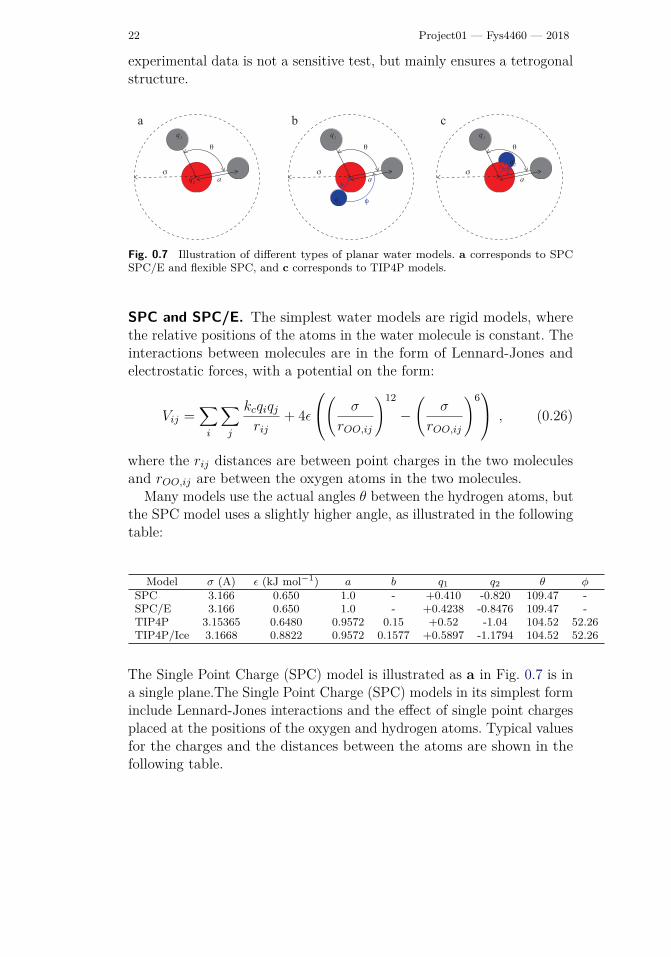
Various aspects of water models are illustrated in Fig. 0.7. The mod-els typically include both electrostatic e�ects from point charges andLennard-Jones e�ects. The Lennard-Jones e�ects ensure that there arerepulsive interactions at short distances so that the structures do notcollapse under electrostatic interactions. The electrostatic interactions in-troduce a component that leads to alignment and directional interactions.Typically, the models have been developed to ensure a good fit to one ora few physical structures or parameters, such as the radial distributionfunction or critical parameters. However, it should be noted that goodcorrespondence for the radial distribution function when compared with

22 Project01 — Fys4460 — 2018

experimental data is not a sensitive test, but mainly ensures a tetrogonalstructure.

a

θ

q1

q2σ

a

a

θ

q1

σ

b

a

θ

q1

σ

c

q2

b

φ

bq2φ

Fig. 0.7 Illustration of di�erent types of planar water models. a corresponds to SPC

SPC/E and flexible SPC, and c corresponds to TIP4P models.

SPC and SPC/E. The simplest water models are rigid models, wherethe relative positions of the atoms in the water molecule is constant. Theinteractions between molecules are in the form of Lennard-Jones andelectrostatic forces, with a potential on the form:

Vij =ÿ

i

ÿ

j

kcqiqj

rij

+ 4‘

Q

aA

‡

rOO,ij

B12

≠A

‡

rOO,ij

B6R

b , (0.26)

where the rij distances are between point charges in the two moleculesand rOO,ij are between the oxygen atoms in the two molecules.

Many models use the actual angles ◊ between the hydrogen atoms, butthe SPC model uses a slightly higher angle, as illustrated in the followingtable:

Model ‡ (A) ‘ (kJ mol≠1

) a b q1 q2 ◊ „SPC 3.166 0.650 1.0 - +0.410 -0.820 109.47 -

SPC/E 3.166 0.650 1.0 - +0.4238 -0.8476 109.47 -

TIP4P 3.15365 0.6480 0.9572 0.15 +0.52 -1.04 104.52 52.26

TIP4P/Ice 3.1668 0.8822 0.9572 0.1577 +0.5897 -1.1794 104.52 52.26

The Single Point Charge (SPC) model is illustrated as a in Fig. 0.7 is ina single plane.The Single Point Charge (SPC) models in its simplest forminclude Lennard-Jones interactions and the e�ect of single point chargesplaced at the positions of the oxygen and hydrogen atoms. Typical valuesfor the charges and the distances between the atoms are shown in thefollowing table.

Project01 — Fys4460 — 2018 23

The SPC/E model is a modified version of the SPC model that alsoincludes an additional average polarization correction in the energy. TheTIP3P model is also a 3-site model, which is slightly modified in theCHARMM force field.

Notice that the parameters may be slightly changed in various forcefield applications. In this case, you should use the modified parameterssince these have been optimized for the types of interactions that areincluded.

Flexible SPE. The flexible SPC model is a bonded model where thebehavior of the O-H and H-O-H bonds are explicitely included andmodeled. The O-H stretching can also be made anharmonic, such as inthe model by Toukan and Rahman, which provides a better descriptionof the dynamical behavior of the system. This model is considered one ofthe most accurate three-site water models without polarization e�ects.

TIP4P. The TIP4P model is an example of an in-plane four-site model.This model is frequently used in many computational chemistry andbiomolecular systems. There have been many reparameterizations of theTIP4P model for various special situations, for example the TIP4P/Icemodel which is particularly suited for modeling ice systems.

ClayFF.Implementing water models in Lammps. Here, we will address watersystems that are modeled using the SPC/E model. In this case, thewater molecules will move as a rigid body. This requires the fix shakecommand in Lammps, which is used to hold the O-H bonds and theH-O-H angles constant.

We will use the moltemplate program to set up water simulations.This is an e�ective tool for setting up and manipulating more complicatedstructures. In particular, it allows us to build structures from a singleunit. Moltemplate includes not only coordinates, topology and force-fieldsettings, but can also include additional information such as the shakeconstraints needed to model rigid molecules.

We will do this by following the example introduced in the moltemplatemanual that sets up a box of SPCE water and runs a simulation on thissystem.

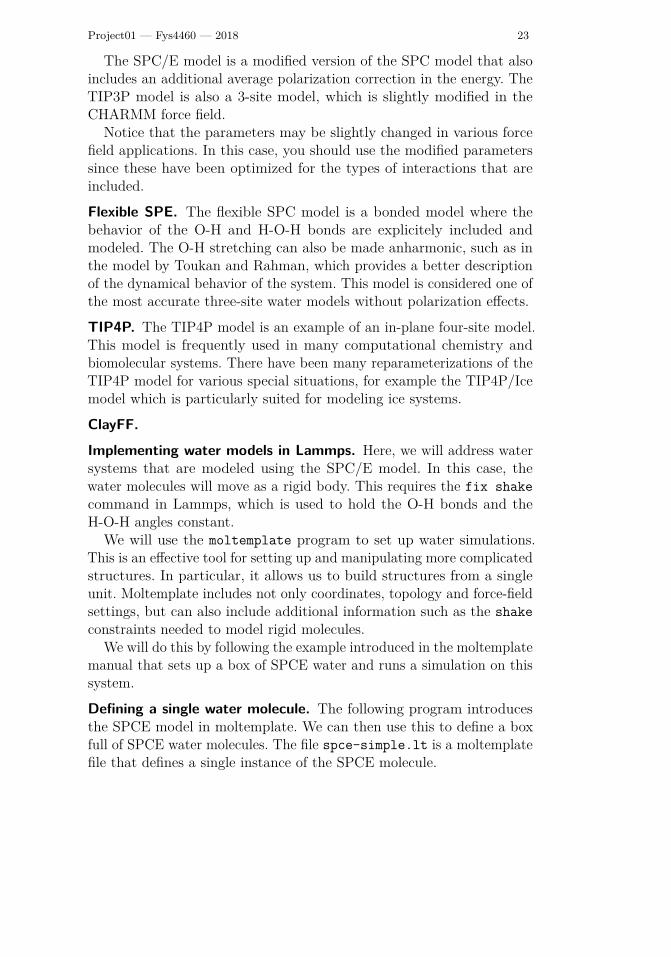
Defining a single water molecule. The following program introducesthe SPCE model in moltemplate. We can then use this to define a boxfull of SPCE water molecules. The file spce-simple.lt is a moltemplatefile that defines a single instance of the SPCE molecule.

24 Project01 — Fys4460 — 2018

# (NOTE: Text following # characters are comments)## file "spce_simple.lt"## H1 H2# \ /# O#SPCE {

# LAMMPS supports a large number of force-field styles. We must select# which ones we need. This information belongs in the "In Init" section.write_once("In Init") {

units real # angstroms, kCal/mole, Daltons, Kelvinatom_style full # select column format for Atoms sectionpair_style lj/cut/coul/long 10.35 # params needed: epsilon sigmabond_style harmonic # parameters needed: k_bond, r0angle_style harmonic # parameters needed: k_theta, theta0kspace_style ewald 0.0001 # long-range electrostatics sum methodpair_modify tail yes

}## Atom properties and molecular topology go in the various "Data ..." sections# We selected "atom_style full". That means we use this column format:# atomID molID atomType charge coordX coordY coordZwrite("Data Atoms") {

$atom:O $mol:. @atom:O -0.8476 0.0000000 0.000000 0.00000$atom:H1 $mol:. @atom:H 0.4238 0.8164904 0.5773590 0.00000$atom:H2 $mol:. @atom:H 0.4238 -0.8164904 0.5773590 0.00000

}# All 3 atoms share same molID number which is unique for each water molecule# The "O" & "H1","H2" atoms in ALL molecules share same atom types: "O" & "H"write_once("Data Masses") {

# atomType mass@atom:O 15.9994@atom:H 1.008

}write("Data Bonds") {

# bondID bondType atomID1 atomID2$bond:OH1 @bond:OH $atom:O $atom:H1$bond:OH2 @bond:OH $atom:O $atom:H2

}write("Data Angles") {

# angleID angleType atomID1 atomID2 atomID3$angle:HOH @angle:HOH $atom:H1 $atom:O $atom:H2

}# --- Force-field parameters go in the "In Settings" section: ---write_once("In Settings") {

# -- Non-bonded (Pair) interactions --# atomType1 atomType2 parameter-list (epsilon, sigma)

pair_coeff @atom:O @atom:O 0.1553 3.5532pair_coeff @atom:H @atom:H 0.0 2.058

# (mixing rules determine interactions between types @atom:O and @atom:H)# -- Bonded interactions --# bondType parameter list (k_bond, r0)

bond_coeff @bond:OH 554.1349 1.0

# angleType parameter-list (k_theta, theta0)

angle_coeff @angle:HOH 45.7696 109.47

Project01 — Fys4460 — 2018 25

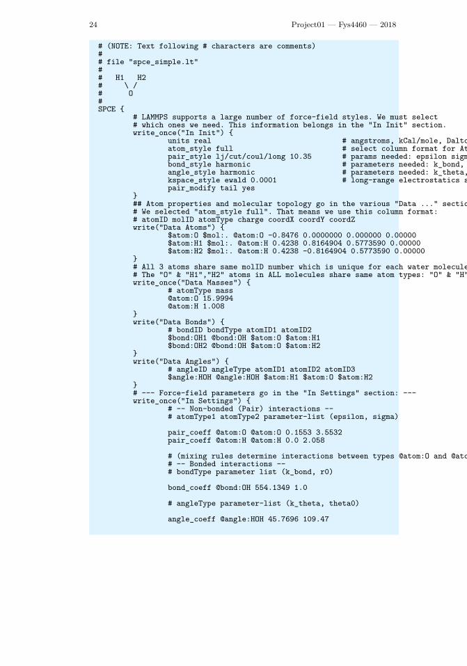
# Group definitions and constraints can also go in the "In Settings" section

group spce type @atom:O @atom:H

#fix fSHAKE spce shake 0.0001 10 100 b @bond:OH a @angle:HOH# (lammps quirk: Remember to "unfix fSHAKE" during minimization.)

}} # SPCE

However, to use this definition, we need to use moltemplate commandsto generate water molecules. We write these commands in a script,spce-water-system.lt, which we then subsequently run to generate aset of files that are used when we run Lammps.

Let us first look at how we generate water molecules and place thenin space. The command

wat1 = new SPCE

generates a single water molecule. We can generate another at a slightlydisplaced position by

wat2 = new SPCE.move(3.450, 0.0, 0.0)wat3 = new SPCE.move(6.900, 0.0, 0.0)

which generates a new molecule at a position translated by 3.450 in thex-direction, and then at 0.6900 in the x-direction. We can simplify thisan generate a 10 ◊ 10 ◊ 10 box using the command

wat = new SPCE [10].move(0,0,3.45)[10].move(0,3.45,0)[10].move(3.45,0,0)

This generates a 10 ◊ 10 ◊ 10 cubic lattice of SPCE water molecules. Thefull script, spce-water-system.lt reads as follows:

# -- file "spce-water-system.lt" --import "spce-simple.lt"

wat = new SPCE [10].move(0,0,3.45)[10].move(0,3.45,0)[10].move(3.45,0,0)

write_once("Data Boundary") {0.0 34.5 xlo xhi0.0 34.5 ylo yhi0.0 34.5 zlo zhi

}

You can generate the files for lammps by running the following com-mand on the command line:

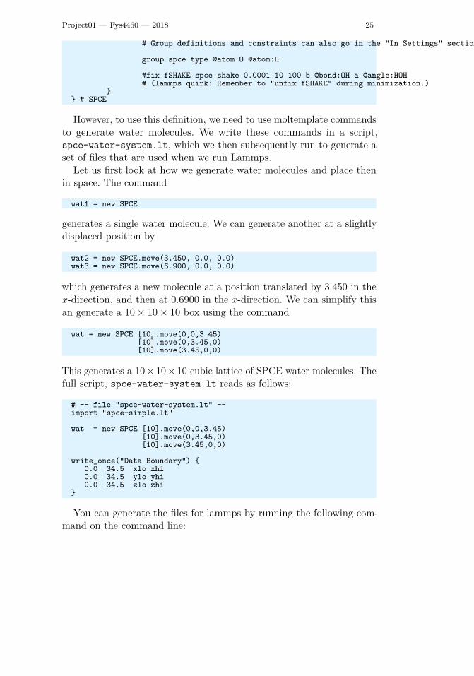
26 Project01 — Fys4460 — 2018

moltemplate.sh -atomstyle "full" spce-water-system.lt

This generates four files: spce-water-system.in, which isthe file to be used by lammps; spce-water-system.data whichis a file that is read by lammps, spce_water_system.in.initand spce-water-system.in.setting, which are included by thespce-water-system.in file. Notice that we also need to specifythe system size, the boundaries of the simulation box, with thewrite_once("Data Boundary") command, which is followed by thesystem size.

The spce-water-system.in file will contain the following:

# ----------------- Init Section -----------------include "spce-water-system.in.init"

# ----------------- Atom Definition Section -----------------read_data "spce-water-system.data"

# ----------------- Settings Section -----------------include "spce-water-system.in.settings"

# ----------------- Run Section -----------------timestep 1.0dump 1 all custom 10 traj_npt.lammpstrj id mol type x y z ix iy izfix fxnpt all npt temp 300.0 300.0 100.0 iso 1.0 1.0 1000.0 drag 1.0thermo 100run 1000

Here, the part in the Run Section have been manually added after-wards to describe the particulars of the simulation. You can now run thisLammps-script using

lmp_serial < spce-water-system.in

and analyse the resulting simulation using Ovito.

m) Characterize the SPCE system using the tools you have developedpreviously. Find g(r) and D(T ) for T over a reasonable range of temper-atures for this system.

n) (Optional) Introduce an additional water model and redo the studyfor this model and compare with your results for SPCE. Comment onsimilarities and di�erences.

Tables of values.Units. In all calculations for the Lennard-Jones system, we will useso-called MD units. These assume that all the particles in a simulationare identical, so the masses and LJ parameters can be factored out of the

Project01 — Fys4460 — 2018 27

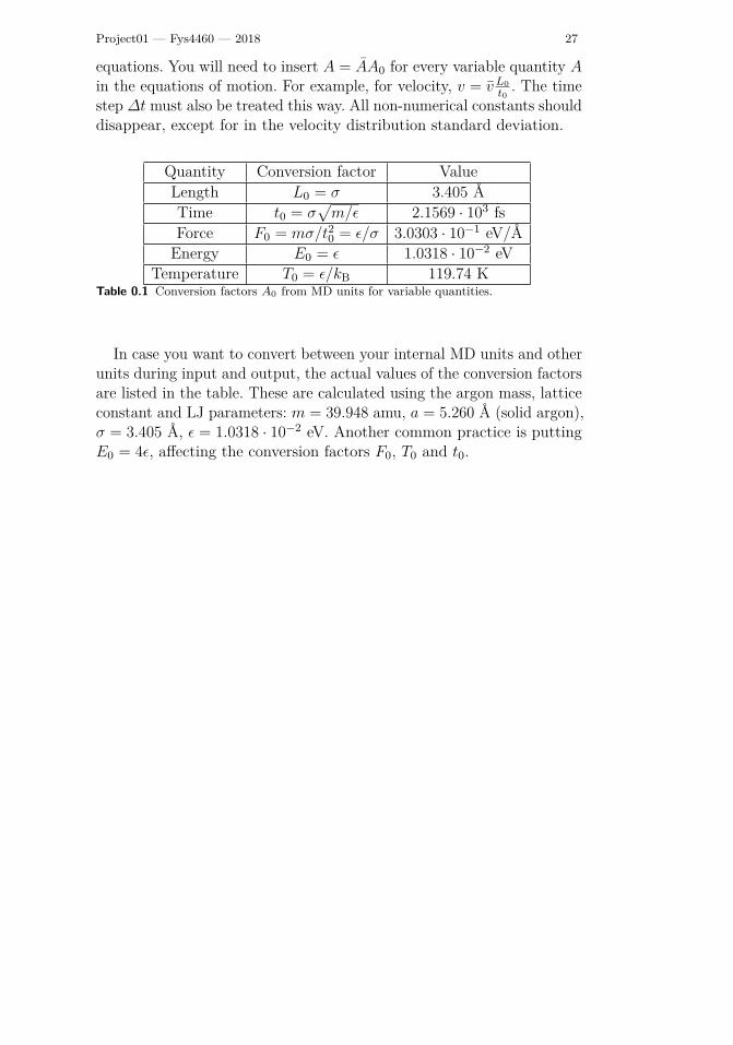
equations. You will need to insert A = AA0 for every variable quantity Ain the equations of motion. For example, for velocity, v = v L0

t0. The time

step ∆t must also be treated this way. All non-numerical constants shoulddisappear, except for in the velocity distribution standard deviation.

Quantity Conversion factor ValueLength L0 = ‡ 3.405 ÅTime t0 = ‡

m/‘ 2.1569 · 103 fs

Force F0 = m‡/t20 = ‘/‡ 3.0303 · 10≠1 eV/Å

Energy E0 = ‘ 1.0318 · 10≠2 eVTemperature T0 = ‘/kB 119.74 K

Table 0.1 Conversion factors A0 from MD units for variable quantities.

In case you want to convert between your internal MD units and otherunits during input and output, the actual values of the conversion factorsare listed in the table. These are calculated using the argon mass, latticeconstant and LJ parameters: m = 39.948 amu, a = 5.260 Å (solid argon),‡ = 3.405 Å, ‘ = 1.0318 · 10≠2 eV. Another common practice is puttingE0 = 4‘, a�ecting the conversion factors F0, T0 and t0.

28 Project01 — Fys4460 — 2018