Project Ahmedawad

S.MANF

Statistical Project Presented by Ahmed Hassan Ibrahim

Presented by Ahmed Hassan Ibrahim

Frequency Distribution

Frequency Distribution

1.1 Raw Data

1.2 Arrays

1.3 Frequency distribution

1.4 Histogram and Frequency Polygons

1.5 The relative Histogram and Frequency Polygons

1.6 Cumulative frequency and Ogives

1.7 Relative Cumulative frequency and percentage

Ogives

1.8 Frequency Curve and Smoothed Ogives

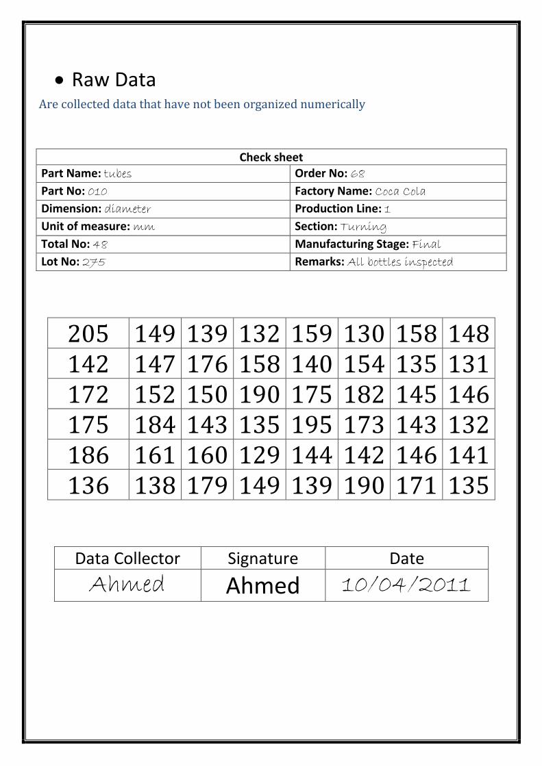
Raw Data Are collected data that have not been organized numerically

205 149 139 132 159 130 158 148 142 147 176 158 140 154 135 131 172 152 150 190 175 182 145 146 175 184 143 135 195 173 143 132 186 161 160 129 144 142 146 141 136 138 179 149 139 190 171 135

Data Collector Signature Date

Ahmed Ahmed 10/04/2011

Check sheet Part Name: tubes Order No: 68

Part No: 010 Factory Name: Coca Cola

Dimension: diameter Production Line: 1

Unit of measure: mm Section: Turning

Total No: 48 Manufacturing Stage: Final

Lot No: 275 Remarks: All bottles inspected

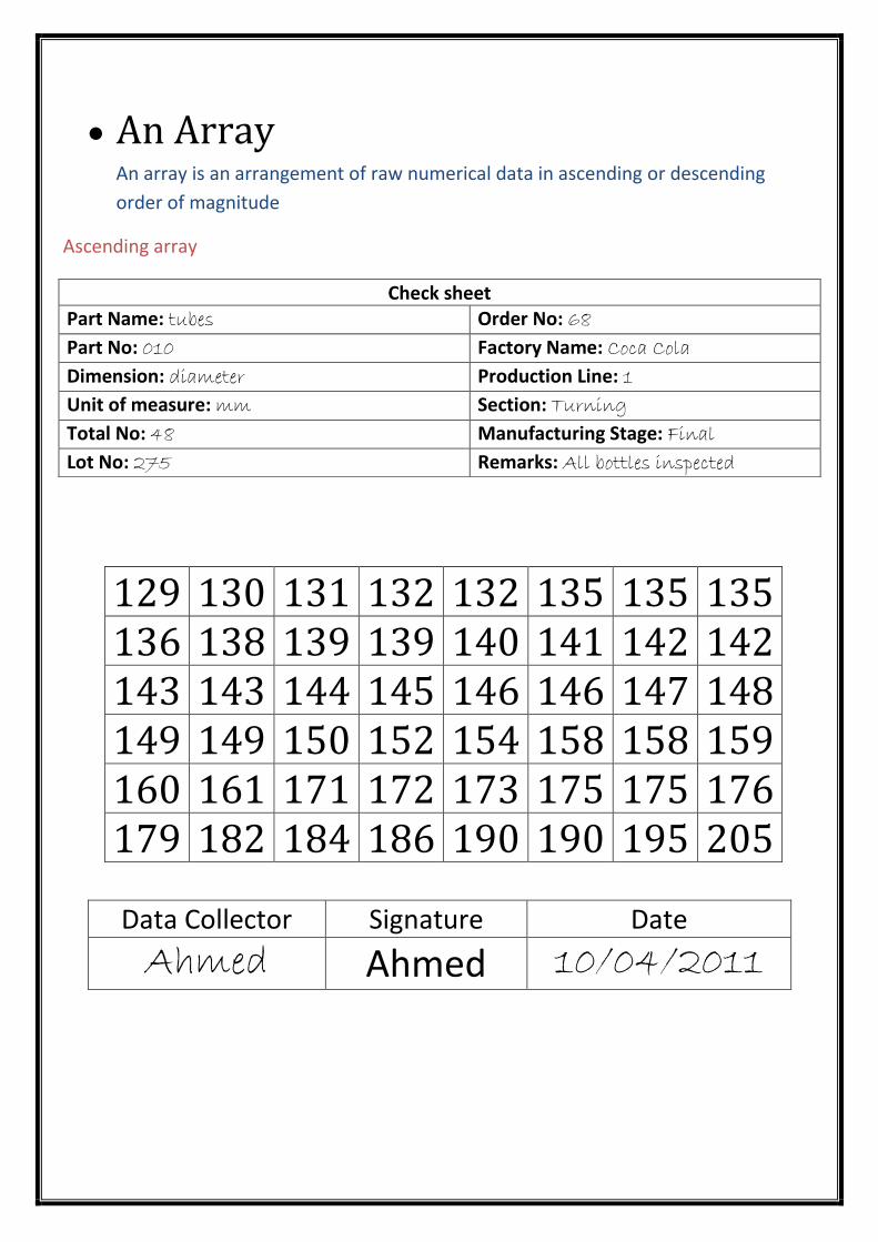
An Array

An array is an arrangement of raw numerical data in ascending or descending

order of magnitude

Ascending array









135 135 135 132 132 131 130 129 142 142 141 140 139 139 138 136 148 147 146 146 145 144 143 143 159 158 158 154 152 150 149 149 176 175 175 173 172 171 161 160 205 195 190 190 186 184 182 179

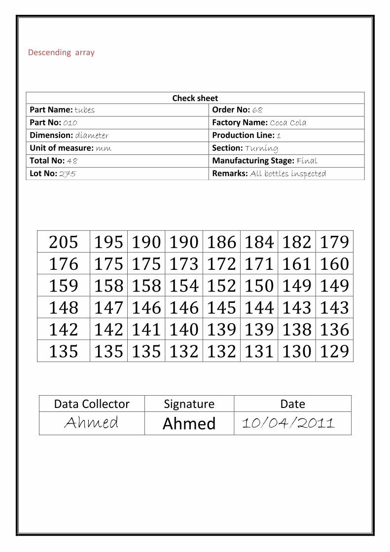
Descending array

205 195 190 190 186 184 182 179 176 175 175 173 172 171 161 160 159 158 158 154 152 150 149 149 148 147 146 146 145 144 143 143 142 142 141 140 139 139 138 136 135 135 135 132 132 131 130 129









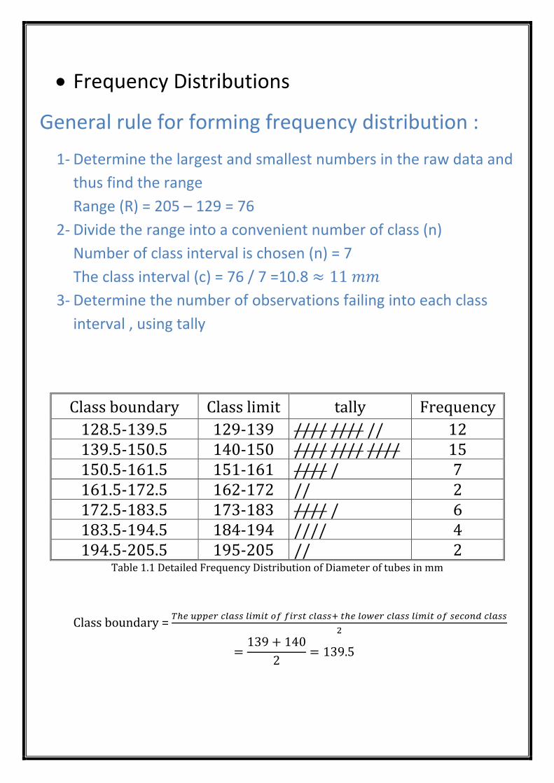
Frequency Distributions

General rule for forming frequency distribution :

1- Determine the largest and smallest numbers in the raw data and

thus find the range

Range (R) = 205 – 129 = 76

2- Divide the range into a convenient number of class (n)

Number of class interval is chosen (n) = 7

The class interval (c) = 76 / 7 =10.8

3- Determine the number of observations failing into each class

interval , using tally

Class boundary Class limit tally Frequency

128.5-139.5 129-139 //// //// // 12 139.5-150.5 140-150 //// //// //// 15 150.5-161.5 151-161 //// / 7 161.5-172.5 162-172 // 2 172.5-183.5 173-183 //// / 6 183.5-194.5 184-194 //// 4 194.5-205.5 195-205 // 2

Table 1.1 Detailed Frequency Distribution of Diameter of tubes in mm

Class boundary =

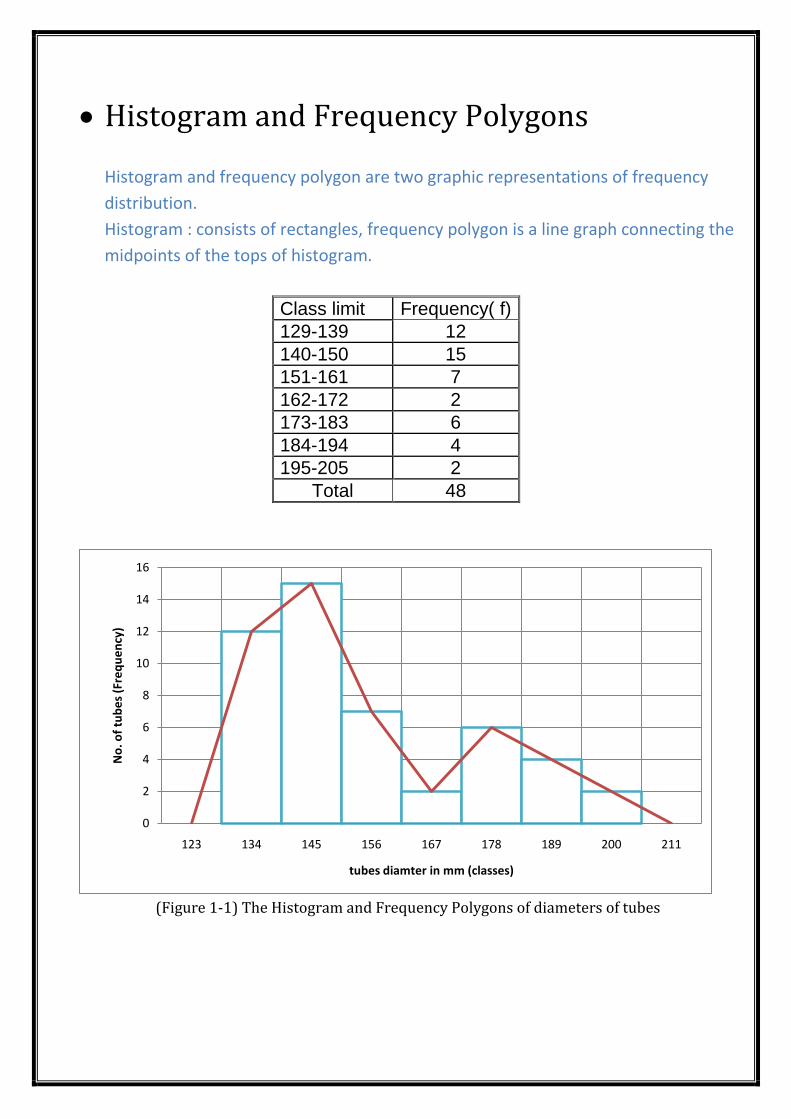
Histogram and Frequency Polygons

Histogram and frequency polygon are two graphic representations of frequency

distribution.

Histogram : consists of rectangles, frequency polygon is a line graph connecting the

midpoints of the tops of histogram.

Class limit Frequency( f)

129-139 12

140-150 15

151-161 7

162-172 2

173-183 6

184-194 4

195-205 2

Total 48

(Figure 1-1) The Histogram and Frequency Polygons of diameters of tubes

0

2

4

6

8

10

12

14

16

123 134 145 156 167 178 189 200 211

No

. of

tub

es

(Fre

qu

en

cy)

tubes diamter in mm (classes)

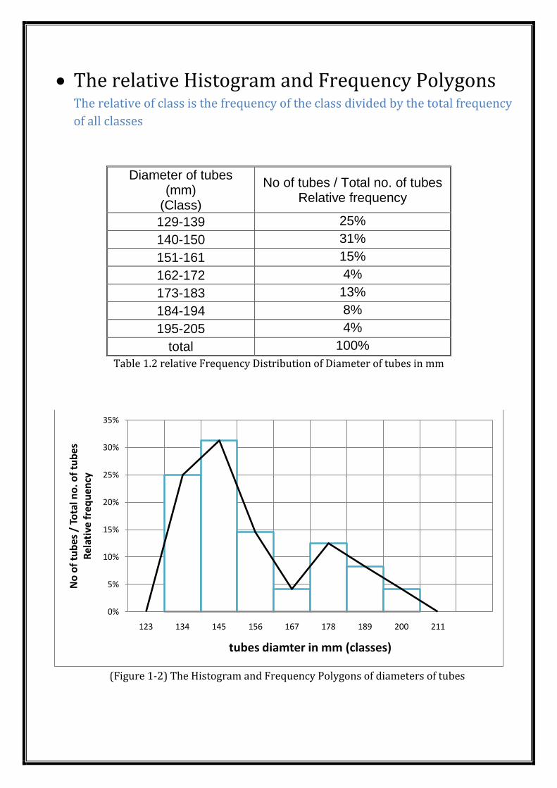
The relative Histogram and Frequency Polygons The relative of class is the frequency of the class divided by the total frequency

of all classes

Diameter of tubes (mm)

(Class)

No of tubes / Total no. of tubes Relative frequency

129-139 25%

140-150 31%

151-161 15%

162-172 4%

173-183 13%

184-194 8%

195-205 4%

total 100%

Table 1.2 relative Frequency Distribution of Diameter of tubes in mm

(Figure 1-2) The Histogram and Frequency Polygons of diameters of tubes

0%

5%

10%

15%

20%

25%

30%

35%

123 134 145 156 167 178 189 200 211

No

of

tub

es /

To

tal n

o. o

f tu

bes

Rel

ativ

e fr

equ

ency


Cumulative frequency and Ogives - Less Than Method

lower than or equal to the upper boundaries of each class interval


No of tubes Cumulative frequency

Less than 128.5 12.00

Less than 139.5 27.00

Less than 150.5 34.00

Less than 161.5 36.00

Less than 172.5 42.00

Less than 183.5 46.00

Less than 194.5 48.00 (Table 1.3) Cumulative frequency Distribution of Diameter of tubes in mm

(Figure 1-3) The Cumulative frequency Polygons of diameters of tubes

"Less Than"

0

10

20

30

40

50

60

123 134 145 156 167 178 189 200 211

Less

Th

an C

um

ula

tive

fre

qu

ency


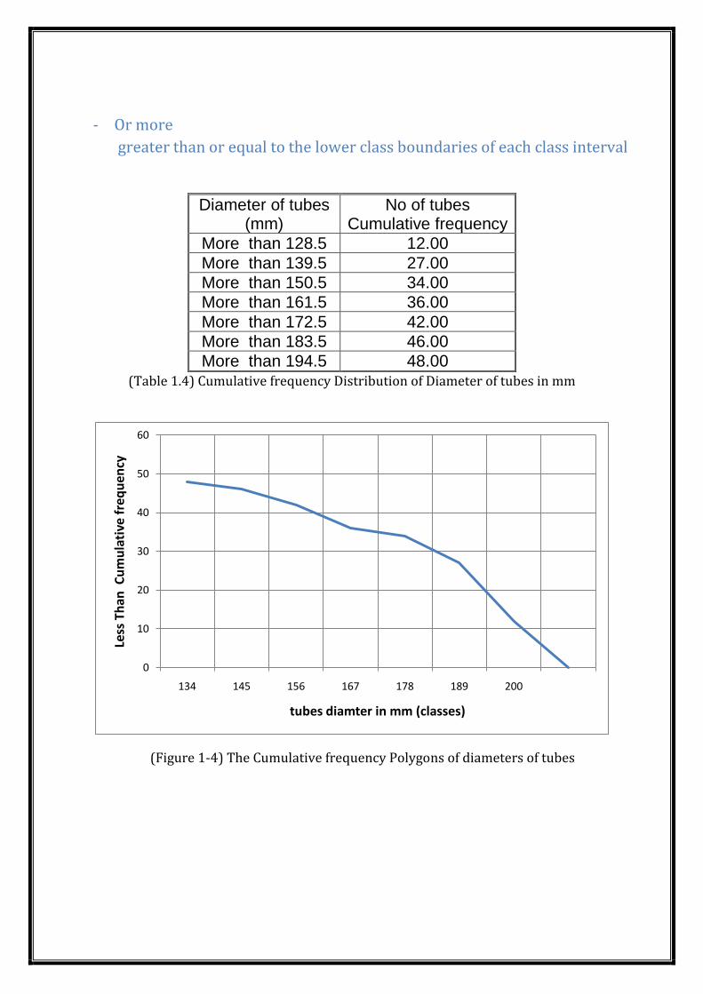
- Or more

greater than or equal to the lower class boundaries of each class interval


No of tubes Cumulative frequency

More than 128.5 12.00

More than 139.5 27.00

More than 150.5 34.00

More than 161.5 36.00

More than 172.5 42.00

More than 183.5 46.00

More than 194.5 48.00 (Table 1.4) Cumulative frequency Distribution of Diameter of tubes in mm

(Figure 1-4) The Cumulative frequency Polygons of diameters of tubes

0

10

20

30

40

50

60

134 145 156 167 178 189 200

Less

Th

an C

um

ula

tive

fre

qu

ency


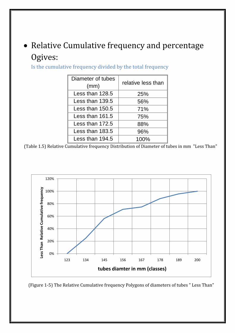
Relative Cumulative frequency and percentage

Ogives: Is the cumulative frequency divided by the total frequency

Diameter of tubes

(mm) relative less than

Less than 128.5 25%

Less than 139.5 56%

Less than 150.5 71%

Less than 161.5 75%

Less than 172.5 88%

Less than 183.5 96%

Less than 194.5 100%

(Table 1.5) Relative Cumulative frequency Distribution of Diameter of tubes in mm "Less Than"

(Figure 1-5) The Relative Cumulative frequency Polygons of diameters of tubes " Less Than"

0%

20%

40%

60%

80%

100%

120%

123 134 145 156 167 178 189 200

Less

Th

an R

elat

ive

Cu

mu

lati

ve fr

equ

ency


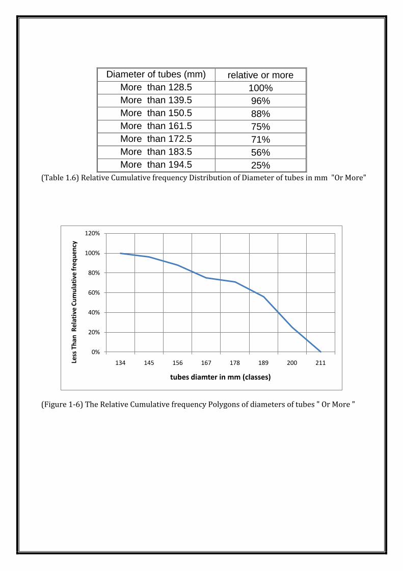
Diameter of tubes (mm) relative or more

More than 128.5 100%

More than 139.5 96%

More than 150.5 88%

More than 161.5 75%

More than 172.5 71%

More than 183.5 56%

More than 194.5 25%

(Table 1.6) Relative Cumulative frequency Distribution of Diameter of tubes in mm "Or More"

(Figure 1-6) The Relative Cumulative frequency Polygons of diameters of tubes " Or More "

0%

20%

40%

60%

80%

100%

120%

134 145 156 167 178 189 200 211Less

Th

an R

elat

ive

Cu

mu

lati

ve fr

equ

ency


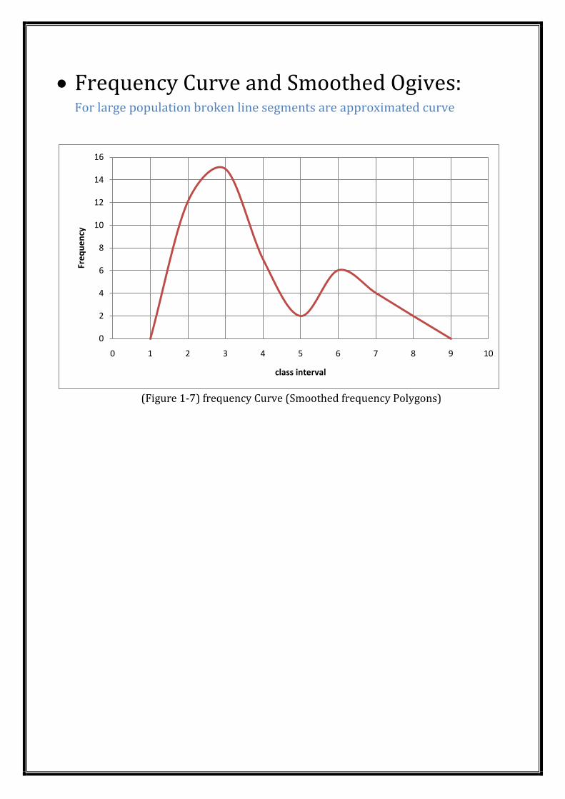
Frequency Curve and Smoothed Ogives: For large population broken line segments are approximated curve

(Figure 1-7) frequency Curve (Smoothed frequency Polygons)

0

2

4

6

8

10

12

14

16

0 1 2 3 4 5 6 7 8 9 10

Fre

qu

en

cy

class interval

Measure of Central Tendency

Measure of Central Tendency

2.1 The Arithmetic Mean

2.2 The Median

2.3 The Mode

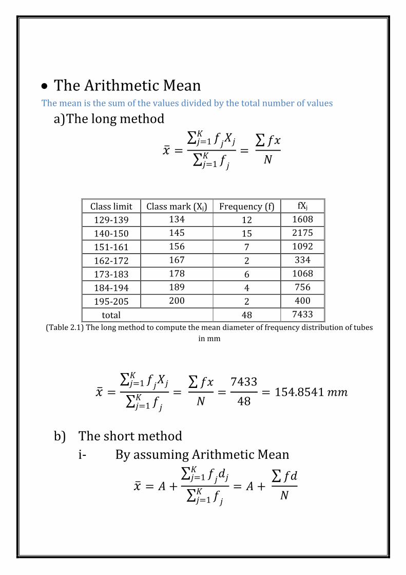
The Arithmetic Mean The mean is the sum of the values divided by the total number of values

a) The long method

Class limit Class mark (Xj) Frequency (f) fXj

129-139 134 12 1608

140-150 145 15 2175

151-161 156 7 1092

162-172 167 2 334

173-183 178 6 1068

184-194 189 4 756

195-205 200 2 400

total 48 7433

(Table 2.1) The long method to compute the mean diameter of frequency distribution of tubes

in mm

b) The short method

i- By assuming Arithmetic Mean

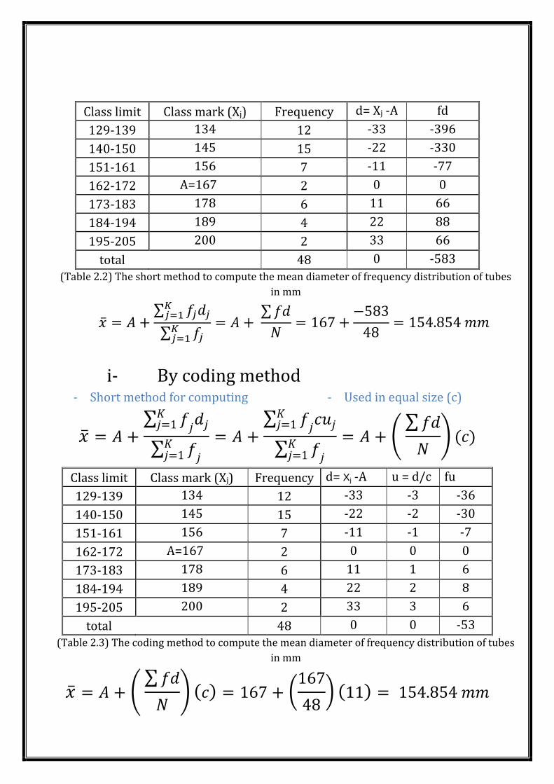
Class limit Class mark (Xj) Frequency d= Xj -A fd

129-139 134 12 -33 -396

140-150 145 15 -22 -330

151-161 156 7 -11 -77

162-172 A=167 2 0 0

173-183 178 6 11 66

184-194 189 4 22 88

195-205 200 2 33 66

total 48 0 -583

(Table 2.2) The short method to compute the mean diameter of frequency distribution of tubes

in mm

i- By coding method - Used in equal size (c) - Short method for computing

Class limit Class mark (Xj) Frequency d= Xj -A u = d/c fu

129-139 134 12 -33 -3 -36

140-150 145 15 -22 -2 -30

151-161 156 7 -11 -1 -7

162-172 A=167 2 0 0 0

173-183 178 6 11 1 6

184-194 189 4 22 2 8

195-205 200 2 33 3 6

total 48 0 0 -53

(Table 2.3) The coding method to compute the mean diameter of frequency distribution of tubes

in mm

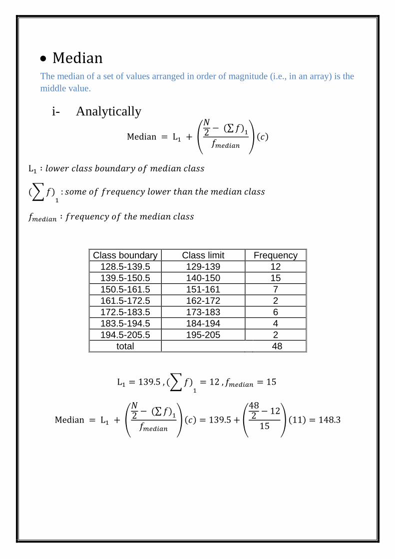
Median The median of a set of values arranged in order of magnitude (i.e., in an array) is the

middle value.

i- Analytically

Class boundary Class limit Frequency

128.5-139.5 129-139 12

139.5-150.5 140-150 15

150.5-161.5 151-161 7

161.5-172.5 162-172 2

172.5-183.5 173-183 6

183.5-194.5 184-194 4

194.5-205.5 195-205 2

total

48

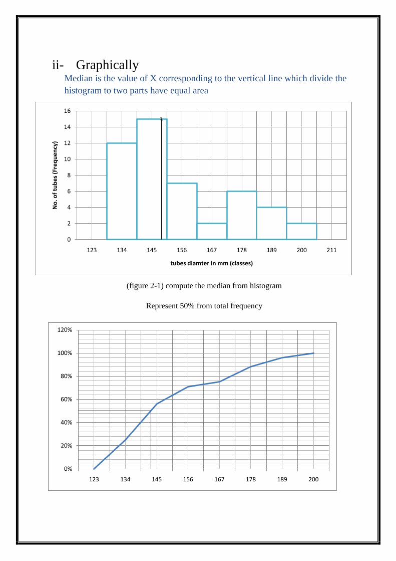
ii- Graphically

Median is the value of X corresponding to the vertical line which divide the

histogram to two parts have equal area

(figure 2-1) compute the median from histogram

Represent 50% from total frequency

0

2

4

6

8

10

12

14

16

123 134 145 156 167 178 189 200 211

No

. of

tub

es

(Fre

qu

en

cy)


0%

20%

40%

60%

80%

100%

120%

123 134 145 156 167 178 189 200

0

2

4

6

8

10

12

14

16

123 134 145 156 167 178 189 200 211

No

. of

tub

es (

Freq

uen

cy)


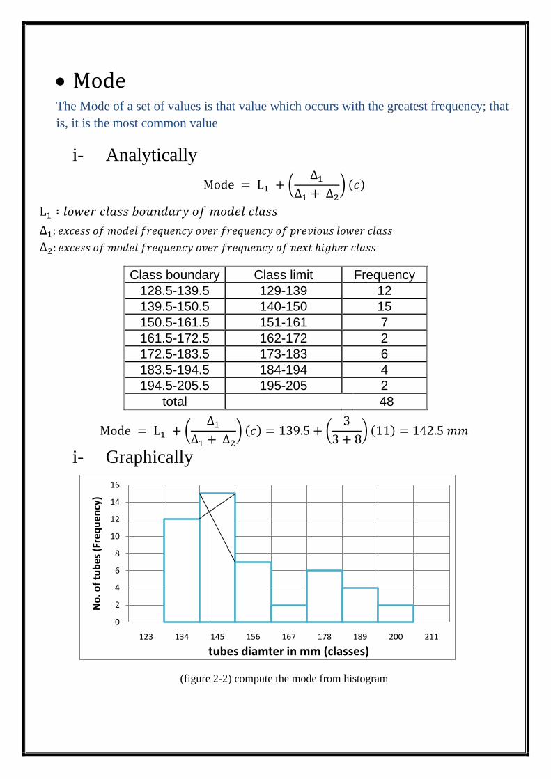
Mode The Mode of a set of values is that value which occurs with the greatest frequency; that

is, it is the most common value

i- Analytically

Class boundary Class limit Frequency

128.5-139.5 129-139 12

139.5-150.5 140-150 15

150.5-161.5 151-161 7

161.5-172.5 162-172 2

172.5-183.5 173-183 6

183.5-194.5 184-194 4

194.5-205.5 195-205 2

total

48

i- Graphically

(figure 2-2) compute the mode from histogram

Measure of Dispersion

Measure of Dispersion

3.1 The Range

3.2 Standard Deviation

3.3 Variance

3.4 coefficient of variation

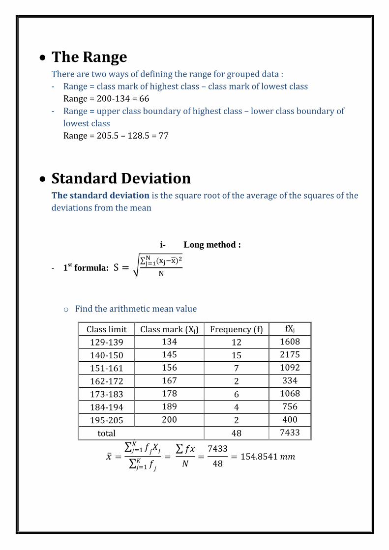
The Range There are two ways of defining the range for grouped data :

- Range = class mark of highest class – class mark of lowest class

Range = 200-134 = 66

- Range = upper class boundary of highest class – lower class boundary of

lowest class

Range = 205.5 – 128.5 = 77

Standard Deviation The standard deviation is the square root of the average of the squares of the

deviations from the mean

i- Long method :

- 1st formula:

o Find the arithmetic mean value

Class limit Class mark (Xj) Frequency (f) fXj

129-139 134 12 1608

140-150 145 15 2175

151-161 156 7 1092

162-172 167 2 334

173-183 178 6 1068

184-194 189 4 756

195-205 200 2 400

total 48 7433

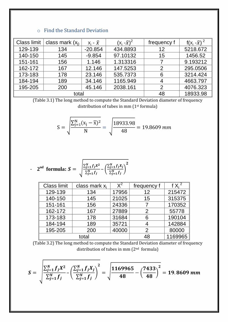
o Find the Standard Deviation

Class limit class mark (xj) Xj - (Xj - )2 frequency f f(Xj - )

2

129-139 134 -20.854 434.8893 12 5218.672

140-150 145 -9.854 97.10132 15 1456.52

151-161 156 1.146 1.313316 7 9.193212

162-172 167 12.146 147.5253 2 295.0506

173-183 178 23.146 535.7373 6 3214.424

184-194 189 34.146 1165.949 4 4663.797

195-205 200 45.146 2038.161 2 4076.323

total 48 18933.98 (Table 3.1) The long method to compute the Standard Deviation diameter of frequency

distribution of tubes in mm (1st formula)

- 2nd

formula:

–

Class limit class mark xj X2 frequency f f Xj 2

129-139 134 17956 12 215472

140-150 145 21025 15 315375

151-161 156 24336 7 170352

162-172 167 27889 2 55778

173-183 178 31684 6 190104

184-194 189 35721 4 142884

195-205 200 40000 2 80000

total 48 1169965 (Table 3.2) The long method to compute the Standard Deviation diameter of frequency

distribution of tubes in mm (2nd formula)

–

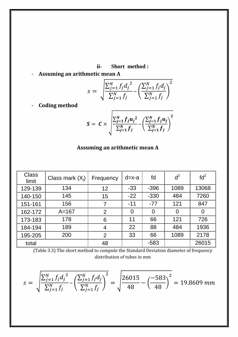
ii- Short method :

- Assuming an arithmetic mean A

–

- Coding method

–

Assuming an arithmetic mean A

Class limit

Class mark (Xj) Frequency d=x-a fd d2 fd2

129-139 134 12 -33 -396 1089 13068

140-150 145 15 -22 -330 484 7260

151-161 156 7 -11 -77 121 847

162-172 A=167 2 0 0 0 0

173-183 178 6 11 66 121 726

184-194 189 4 22 88 484 1936

195-205 200 2 33 66 1089 2178

total 48 -583 26015

(Table 3.3) The short method to compute the Standard Deviation diameter of frequency

distribution of tubes in mm

–

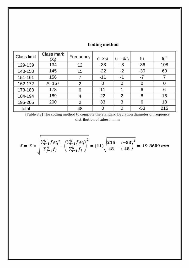
Coding method

Class limit Class mark

(Xj) Frequency d=x-a u = d/c fu fu2

129-139 134 12 -33 -3 -36 108

140-150 145 15 -22 -2 -30 60

151-161 156 7 -11 -1 -7 7

162-172 A=167 2 0 0 0 0

173-183 178 6 11 1 6 6

184-194 189 4 22 2 8 16

195-205 200 2 33 3 6 18

total 48 0 0 -53 215

(Table 3.3) The coding method to compute the Standard Deviation diameter of frequency

distribution of tubes in mm

–

Variance

The variance is the average of the squares of the deviations from the mean.

Long method

i- 1st formula

–

–

ii- 2nd formula

–

–

Short method

i- Assuming an arithmetic mean A

–

–

ii- Coding method

–

–

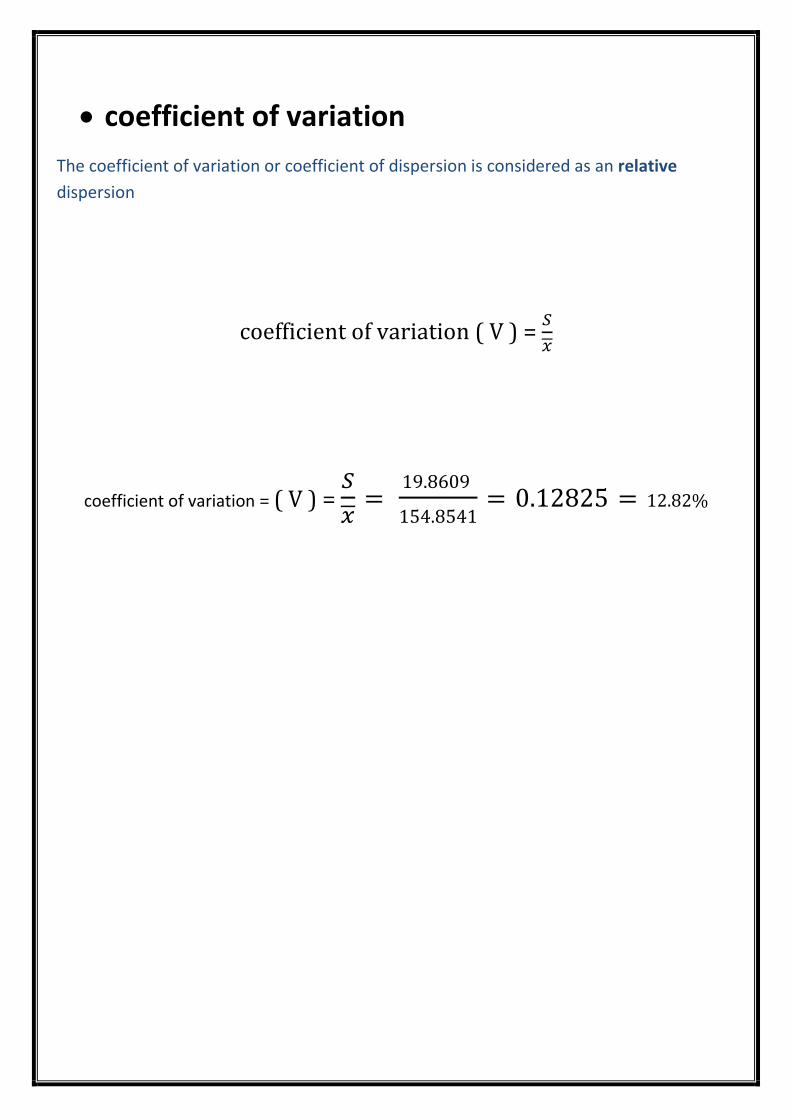
coefficient of variation

The coefficient of variation or coefficient of dispersion is considered as an relative

dispersion

coefficient of variation ( V ) =

coefficient of variation = ( V ) =

Moments, Skewness, Kurtosis

Moments, Skewness, Kurtosis

4.1 Moments 4.2 Skewness

4.3 Kurtosis

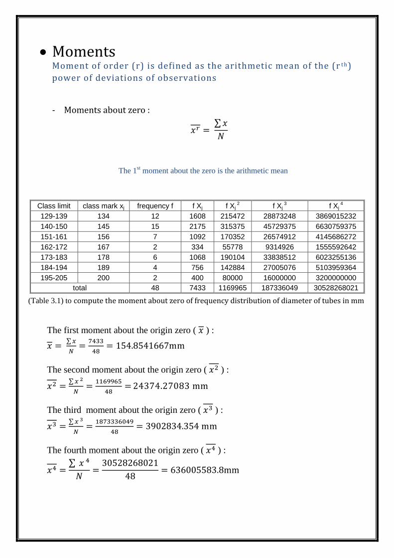
Moments Moment of order (r) is defined as the arithmetic mean of the (r th)

power of deviations of observations

- Moments about zero :

The 1st moment about the zero is the arithmetic mean

Class limit class mark xj frequency f f Xj f Xj 2 f Xj

3 f Xj 4

129-139 134 12 1608 215472 28873248 3869015232

140-150 145 15 2175 315375 45729375 6630759375

151-161 156 7 1092 170352 26574912 4145686272

162-172 167 2 334 55778 9314926 1555592642

173-183 178 6 1068 190104 33838512 6023255136

184-194 189 4 756 142884 27005076 5103959364

195-205 200 2 400 80000 16000000 3200000000

total 48 7433 1169965 187336049 30528268021

(Table 3.1) to compute the moment about zero of frequency distribution of diameter of tubes in mm

The first moment about the origin zero ( ) :

mm

The second moment about the origin zero ( ) :

24374.27083 mm

The third moment about the origin zero ( ) :

mm

The fourth moment about the origin zero ( ) :

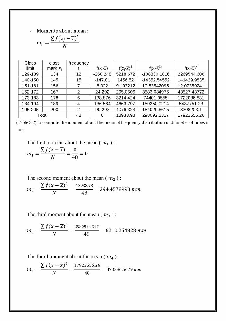
- Moments about mean :

Class limit

class mark Xj

frequency f f(xj- ) f(xj- )2 f(xj-

)3 f(xj- )4

129-139 134 12 -250.248 5218.672 -108830.1816 2269544.606

140-150 145 15 -147.81 1456.52 -14352.54552 141429.9835

151-161 156 7 8.022 9.193212 10.53542095 12.07359241

162-172 167 2 24.292 295.0506 3583.684976 43527.43772

173-183 178 6 138.876 3214.424 74401.0555 1722086.831

184-194 189 4 136.584 4663.797 159250.0214 5437751.23

195-205 200 2 90.292 4076.323 184029.6615 8308203.1

Total 48 0 18933.98 298092.2317 17922555.26

(Table 3.2) to compute the moment about the mean of frequency distribution of diameter of tubes in

mm

The first moment about the mean ( ) :

The second moment about the mean ( ) :

The third moment about the mean ( ) :

The fourth moment about the mean ( ) :

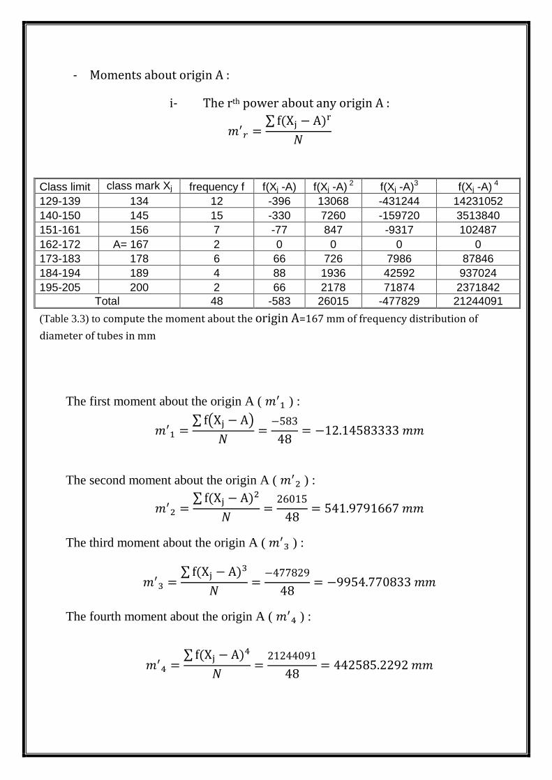
- Moments about origin A :

i- The rth power about any origin A :

Class limit class mark Xj frequency f f(Xj -A) f(Xj -A) 2 f(Xj -A)3 f(Xj -A) 4

129-139 134 12 -396 13068 -431244 14231052

140-150 145 15 -330 7260 -159720 3513840

151-161 156 7 -77 847 -9317 102487

162-172 A= 167 2 0 0 0 0

173-183 178 6 66 726 7986 87846

184-194 189 4 88 1936 42592 937024

195-205 200 2 66 2178 71874 2371842

Total 48 -583 26015 -477829 21244091

(Table 3.3) to compute the moment about the origin A=167 mm of frequency distribution of

diameter of tubes in mm

The first moment about the origin A ( ) :

The second moment about the origin A ( ) :

The third moment about the origin A ( ) :

The fourth moment about the origin A ( ) :

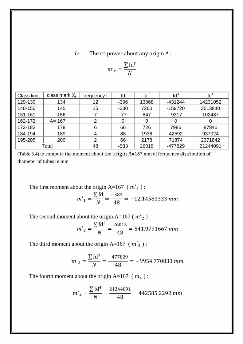
ii- The rth power about any origin A :

Class limit class mark Xj frequency f fd fd 2 fd3 fd4

129-139 134 12 -396 13068 -431244 14231052

140-150 145 15 -330 7260 -159720 3513840

151-161 156 7 -77 847 -9317 102487

162-172 A= 167 2 0 0 0 0

173-183 178 6 66 726 7986 87846

184-194 189 4 88 1936 42592 937024

195-205 200 2 66 2178 71874 2371842

Total 48 -583 26015 -477829 21244091


diameter of tubes in mm

The first moment about the origin A=167 ( ) :

The second moment about the origin A=167 ( ) :

The third moment about the origin A=167 ( ) :

The fourth moment about the origin A=167 ( ) :

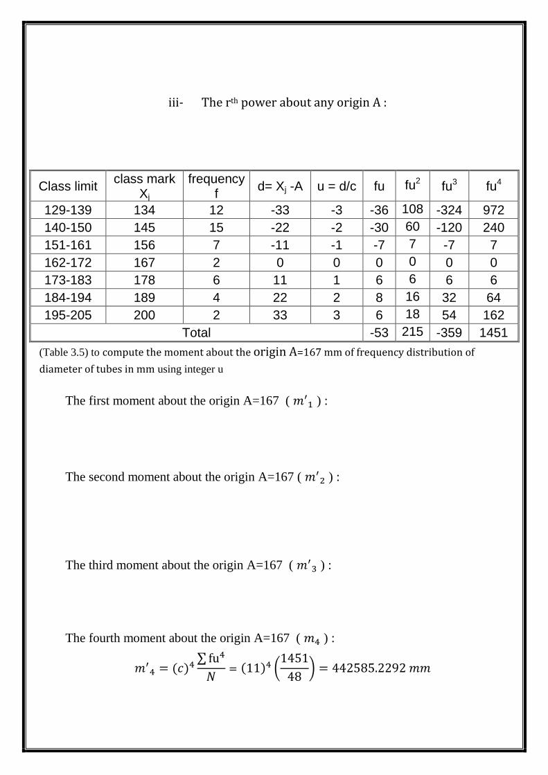
iii- The rth power about any origin A :

Class limit class mark

Xj frequency

f d= Xj -A u = d/c fu fu2 fu3 fu4

129-139 134 12 -33 -3 -36 108 -324 972

140-150 145 15 -22 -2 -30 60 -120 240

151-161 156 7 -11 -1 -7 7 -7 7

162-172 167 2 0 0 0 0 0 0

173-183 178 6 11 1 6 6 6 6

184-194 189 4 22 2 8 16 32 64

195-205 200 2 33 3 6 18 54 162

Total -53 215 -359 1451


diameter of tubes in mm using integer u

The first moment about the origin A=167 ( ) :

The second moment about the origin A=167 ( ) :

The third moment about the origin A=167 ( ) :

The fourth moment about the origin A=167 ( ) :

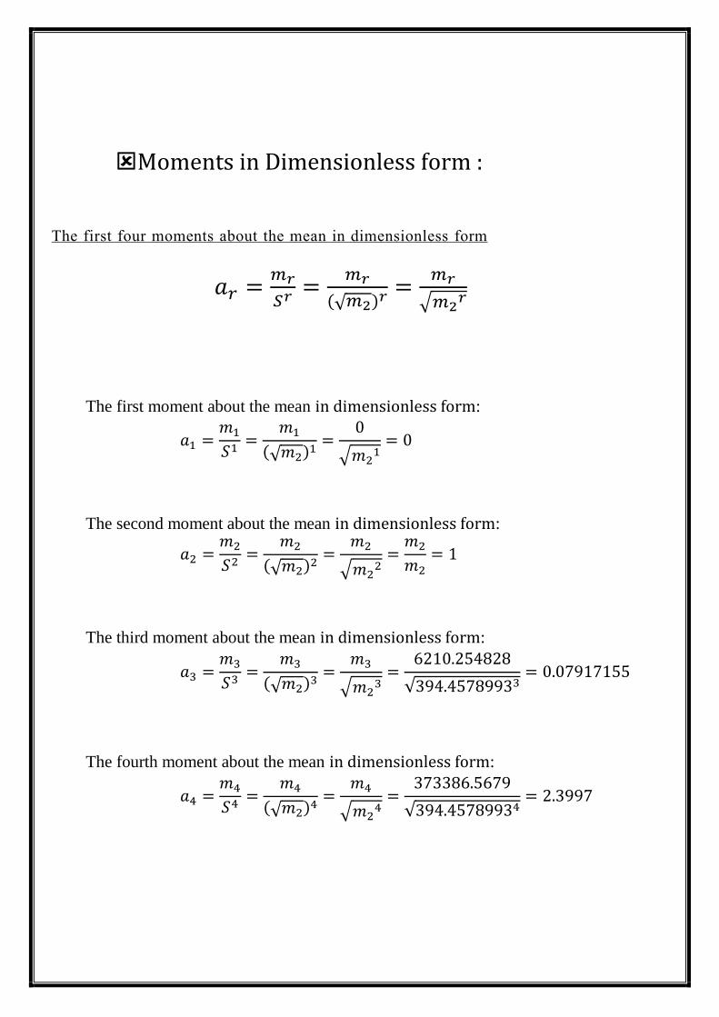
Moments in Dimensionless form :

The first four moments about the mean in dimensionless form

The first moment about the mean in dimensionless form:

The second moment about the mean in dimensionless form:

The third moment about the mean in dimensionless form:

The fourth moment about the mean in dimensionless form:

Skewness

Skewness is defined as the departure from symmetry

–

–

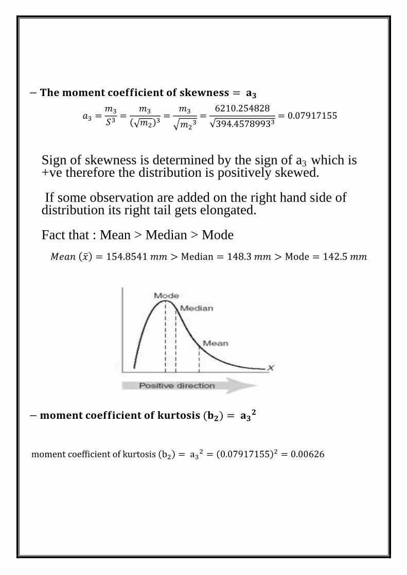
Sign of skewness is determined by the sign of a3 which is +ve therefore the distribution is positively skewed. If some observation are added on the right hand side of distribution its right tail gets elongated. Fact that : Mean > Median > Mode

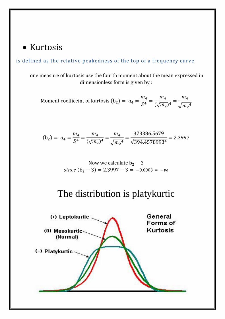
Kurtosis

is defined as the relative peakedness of the top of a frequency curve

one measure of kurtosis use the fourth moment about the mean expressed in

dimensionless form is given by :

Now we calculate

The distribution is platykurtic

Documents

Project Ahmedawad