Project Analysis - kuswanto.staff.gunadarma.ac.idkuswanto.staff.gunadarma.ac.id/Downloads/files/60502/CHAPTER-10.pdf · and maybe some further work on the test bed would confirm the

● ● ● ● ●

confirming pages

240

PART 3 CHAPTER

Project Analysis

10 ◗ Having read our earlier chapters on capital budgeting, you may have concluded that the choice of which projects to accept or reject is a simple one. You just need to draw up a set of cash-flow forecasts, choose the right discount rate, and crank out net present value. But finding projects that create value for the shareholders can never be reduced to a mechanical exercise. We therefore devote the next three chapters to ways in which companies can stack the odds in their favor when making investment decisions.

Investment proposals may emerge from many different parts of the organization. So companies need procedures to ensure that every project is assessed consistently. Our first task in this chapter is to review how firms develop plans and budgets for capital investments, how they authorize specific projects, and how they check whether projects perform as promised.

When managers are presented with investment proposals, they do not accept the cash flow forecasts at face value. Instead, they try to understand what makes a project tick and what could go wrong with it. Remember Murphy’s law, “if anything can go wrong, it will,” and O’Reilly’s corollary, “at the worst possible time.”

Once you know what makes a project tick, you may be able to reconfigure it to improve its chance of success. And if you understand why the venture could fail, you can decide whether it is worth trying to rule out the possible causes of failure. Maybe further expenditure on market research would clear up those doubts about

acceptance by consumers, maybe another drill hole would give you a better idea of the size of the ore body, and maybe some further work on the test bed would confirm the durability of those welds.

If the project really has a negative NPV, the sooner you can identify it, the better. And even if you decide that it is worth going ahead without further analysis, you do not want to be caught by surprise if things go wrong later. You want to know the danger signals and the actions that you might take.

Our second task in this chapter is to show how managers use sensitivity analysis, break-even analysis, and Monte Carlo simulation to identify the crucial assumptions in investment proposals and to explore what can go wrong. There is no magic in these techniques, just computer-assisted common sense. You do not need a license to use them.

Discounted-cash-flow analysis commonly assumes that companies hold assets passively, and it ignores the opportunities to expand the project if it is successful or to bail out if it is not. However, wise managers recognize these opportunities when considering whether to invest. They look for ways to capitalize on success and to reduce the costs of failure, and they are prepared to pay up for projects that give them this flexibility. Opportunities to modify projects as the future unfolds are known as real options. In the final section of the chapter we describe several important real options, and we show how to use decision trees to set out the possible future choices.

BEST PRACTICES IN CAPITAL BUDGETING

● ● ● ● ●

bre30735_ch10_240-267.indd 240bre30735_ch10_240-267.indd 240 12/2/09 5:32:49 PM12/2/09 5:32:49 PM

confirming pages

Chapter 10 Project Analysis 241

Senior management needs some forewarning of future investment outlays. So for most large firms, the investment process starts with the preparation of an annual capital budget, which is a list of investment projects planned for the coming year.

Most firms let project proposals bubble up from plants for review by divisional manage-ment and then from divisions for review by senior management and their planning staff. Of course middle managers cannot identify all worthwhile projects. For example, the managers of plants A and B cannot be expected to see the potential economies of closing their plants and consolidating production at a new plant C. Divisional managers would propose plant C. But the managers of divisions 1 and 2 may not be eager to give up their own computers to a corporation-wide information system. That proposal would come from senior manage-ment, for example, the company’s chief information officer.

Inconsistent assumptions often creep into expenditure plans. For example, suppose the manager of your furniture division is bullish on housing starts, but the manager of your appliance division is bearish. The furniture division may push for a major investment in new facilities, while the appliance division may propose a plan for retrenchment. It would be better if both managers could agree on a common estimate of housing starts and base their investment proposals on it. That is why many firms begin the capital budgeting process by establishing consensus forecasts of economic indicators, such as inflation and growth in national income, as well as forecasts of particular items that are important to the firm’s business, such as housing starts or the prices of raw materials. These forecasts are then used as the basis for the capital budget.

Preparation of the capital budget is not a rigid, bureaucratic exercise. There is plenty of give-and-take and back-and-forth. Divisional managers negotiate with plant managers and fine-tune the division’s list of projects. The final capital budget must also reflect the corporation’s strategic planning. Strategic planning takes a top-down view of the company. It attempts to identify businesses where the company has a competitive advantage. It also attempts to identify businesses that should be sold or allowed to run down.

A firm’s capital investment choices should reflect both bottom-up and top-down views of the business—capital budgeting and strategic planning, respectively. Plant and division managers, who do most of the work in bottom-up capital budgeting, may not see the for-est for the trees. Strategic planners may have a mistaken view of the forest because they do not look at the trees one by one. (We return to the links between capital budgeting and corporate strategy in the next chapter.)

Project Authorizations—and the Problem of Biased Forecasts Once the capital budget has been approved by top management and the board of directors, it is the official plan for the ensuing year. However, it is not the final sign-off for specific projects. Most companies require appropriation requests for each proposal. These requests include detailed forecasts, discounted-cash-flow analyses, and back-up information.

Many investment projects carry a high price tag; they also determine the shape of the firm’s business 10 or 20 years in the future. Hence final approval of appropriation requests tends to be reserved for top management. Companies set ceilings on the size of projects that divisional managers can authorize. Often these ceilings are surprisingly low. For exam-ple, a large company, investing $400 million per year, might require top management to approve all projects over $500,000.

This centralized decision making brings its problems: Senior management can’t process detailed information about hundreds of projects and must rely on forecasts put together by project sponsors. A smart manager quickly learns to worry whether these forecasts are realistic.

10-1 The Capital Investment Process


confirming pages

242 Part Three Best Practices in Capital Budgeting

Even when the forecasts are not consciously inflated, errors creep in. For example, most people tend to be overconfident when they forecast. Events they think are almost certain to occur may actually happen only 80% of the time, and events they believe are impossible may happen 20% of the time. Therefore project risks are understated. Anyone who is keen to get a project accepted is also likely to look on the bright side when forecasting the project’s cash flows. Such overoptimism seems to be a common feature in financial forecasts. Overoptimism afflicts governments too, probably more than private businesses. How often have you heard of a new dam, highway, or military aircraft that actually cost less than was originally forecasted?

You can expect plant or divisional managers to look on the bright side when putting for-ward investment proposals. That is not altogether bad. Psychologists stress that optimism and confidence are likely to increase effort, commitment, and persistence. The problem is that hundreds of appropriation requests may reach senior management each year, all essen-tially sales documents presented by united fronts and designed to persuade. Alternative schemes have been filtered out at earlier stages.

It is probably impossible to eliminate bias completely, but senior managers should take care not to encourage it. For example, if managers believe that success depends on having the largest division rather than the most profitable one, they will propose large expansion projects that they do not truly believe have positive NPVs. Or if new plant managers are pushed to generate increased earnings right away, they will be tempted to propose quick-payback projects even when NPV is sacrificed.

Sometimes senior managers try to offset bias by increasing the hurdle rate for capital expenditure. Suppose the true cost of capital is 10%, but the CFO is frustrated by the large fraction of projects that don’t earn 10%. She therefore directs project sponsors to use a 15% discount rate. In other words, she adds a 5% fudge factor in an attempt to offset forecast bias. But it doesn’t work; it never works. Brealey, Myers, and Allen’s Second Law 1 explains why. The law states: The proportion of proposed projects having positive NPVs at the corporate hurdle rate is independent of the hurdle rate.

The law is not a facetious conjecture. It was tested in a large oil company where staff kept careful statistics on capital investment projects. About 85% of projects had positive NPVs. (The remaining 15% were proposed for other reasons, for example, to meet environmental standards.) One year, after several quarters of disappointing earnings, top management decided that more financial discipline was called for and increased the corporate hurdle rate by several percentage points. But in the following year the fraction of projects with positive NPVs stayed rock-steady at 85%.

If you’re worried about bias in forecasted cash flows, the only remedy is careful analysis of the forecasts. Do not add fudge factors to the cost of capital. 2

Postaudits Most firms keep a check on the progress of large projects by conducting postaudits shortly after the projects have begun to operate. Postaudits identify problems that need fixing, check the accuracy of forecasts, and suggest questions that should have been asked before the project was undertaken. Postaudits pay off mainly by helping managers to do a bet-ter job when it comes to the next round of investments. After a postaudit the controller may say, “We should have anticipated the extra training required for production workers.” When the next proposal arrives, training will get the attention it deserves.

1 There is no First Law. We think “Second Law” sounds better. There is a Third Law, but that is for another chapter. 2 Adding a fudge factor to the cost of capital also favors quick-payback projects and penalizes longer-lived projects, which tend to have lower rates of return but higher NPVs. Adding a 5% fudge factor to the discount rate is roughly equivalent to reducing the forecast and present value of the first year’s cash flow by 5%. The impact on the present value of a cash flow 10 years in the future is much greater, because the fudge factor is compounded in the discount rate. The fudge factor is not too much of a burden for a 2- or 3-year project, but an enormous burden for a 10- or 20-year project.


confirming pages


Postaudits may not be able to measure all of a project’s costs and benefits. It may be impossible to split the project away from the rest of the business. Suppose that you have just taken over a trucking firm that operates a delivery service for local stores. You decide to improve service by installing custom software to keep track of packages and to schedule trucks. You also construct a dispatching center and buy five new diesel trucks. A year later you try a postaudit of the investment in software. You verify that it is working properly and check actual costs of purchase, installation, and operation against projections. But how do you identify the incremental cash inflows? No one has kept records of the extra diesel fuel that would have been used or the extra shipments that would have been lost absent the software. You may be able to verify that service is better, but how much of the improvement comes from the new trucks, how much from the dispatching center, and how much from the soft-ware? The only meaningful measures of success are for the delivery business as a whole.

Uncertainty means that more things can happen than will happen. Whenever you are con-fronted with a cash-flow forecast, you should try to discover what else can happen.

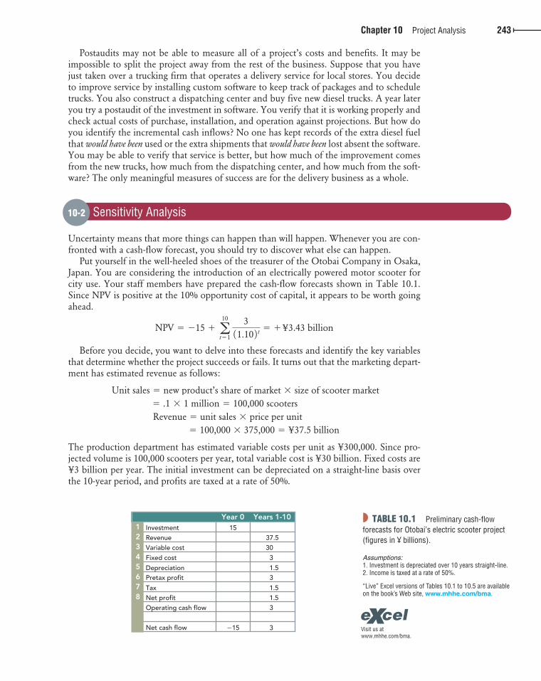
Put yourself in the well-heeled shoes of the treasurer of the Otobai Company in Osaka, Japan. You are considering the introduction of an electrically powered motor scooter for city use. Your staff members have prepared the cash-flow forecasts shown in Table 10.1 . Since NPV is positive at the 10% opportunity cost of capital, it appears to be worth going ahead.

NPV 5 215 1 a10

t51

311.10 2 t

5 1 ¥3.43 billion

Before you decide, you want to delve into these forecasts and identify the key variables that determine whether the project succeeds or fails. It turns out that the marketing depart-ment has estimated revenue as follows:

Unit sales 5 new product’s share of market 3 size of scooter market5 .1 3 1 million 5 100,000 scooters Revenue 5 unit sales 3 price per unit

5 100,000 3 375,000 5 ¥37.5 billion

The production department has estimated variable costs per unit as ¥300,000. Since pro-jected volume is 100,000 scooters per year, total variable cost is ¥30 billion. Fixed costs are ¥3 billion per year. The initial investment can be depreciated on a straight-line basis over the 10-year period, and profits are taxed at a rate of 50%.

10-2 Sensitivity Analysis

◗ TABLE 10.1 Preliminary cash-flow forecasts for Otobai’s electric scooter project (figures in ¥ billions).

Assumptions: 1. Investment is depreciated over 10 years straight-line. 2. Income is taxed at a rate of 50%.

“Live” Excel versions of Tables 10.1 to 10.5 are available on the book’s Web site, www.mhhe.com/bma .

Visit us atwww.mhhe.com/bma.

InvestmentRevenueVariable cost

Fixed cost

DepreciationPretax profit

TaxNet profitOperating cash flow

12345678

Net cash flow

Year 0 Years 1-10

37.530

3

1.53

1.51.53

3

15

�15


confirming pages


These seem to be the important things you need to know, but look out for unidentified variables. Perhaps there are patent problems, or perhaps you will need to invest in ser-vice stations that will recharge the scooter batteries. The greatest dangers often lie in these unknown unknowns, or “unk-unks,” as scientists call them.

Having found no unk-unks (no doubt you will find them later), you conduct a sensitiv-ity analysis with respect to market size, market share, and so on. To do this, the marketing and production staffs are asked to give optimistic and pessimistic estimates for the underly-ing variables. These are set out in the left-hand columns of Table 10.2 . The right-hand side shows what happens to the project’s net present value if the variables are set one at a time to their optimistic and pessimistic values. Your project appears to be by no means a sure thing. The most dangerous variables are market share and unit variable cost. If market share is only .04 (and all other variables are as expected), then the project has an NPV of �¥10.4 billion. If unit variable cost is ¥360,000 (and all other variables are as expected), then the project has an NPV of �¥15 billion.

Value of Information Now you can check whether you could resolve some of the uncertainty before your company parts with the ¥15 billion investment. Suppose that the pessimistic value for unit variable cost partly reflects the production department’s worry that a particular machine will not work as designed and that the operation will have to be performed by other methods at an extra cost of ¥20,000 per unit. The chance that this will occur is only 1 in 10. But, if it does occur, the extra ¥20,000 unit cost will reduce after-tax cash flow by

Unit sales 3 additional unit cost 3 11 2 tax rate 2

5 100,000 3 20,000 3 .50 5 ¥1 billion

It would reduce the NPV of your project by

a10

t51

111.10 2 t

5 ¥6.14 billion,

putting the NPV of the scooter project underwater at � 3.43 � 6.14 � �¥2.71 billion. It is possible that a relatively small change in the scooter’s design would remove the need for the new machine. Or perhaps a ¥10 million pretest of the machine will reveal whether it will work and allow you to clear up the problem. It clearly pays to invest ¥10 million to avoid a 10% probability of a ¥6.14 billion fall in NPV. You are ahead by �10 � .10 � 6,140 � � ¥604 million.

On the other hand, the value of additional information about market size is small. Because the project is acceptable even under pessimistic assumptions about market size, you are unlikely to be in trouble if you have misestimated that variable.

◗ TABLE 10.2 To undertake a sensitivity analysis of the electric scooter project, we set each variable in turn at its most pessimistic or optimistic value and recalculate the NPV of the project.


Range NPV, ¥ billionsExpected ExpectedVariable Pessimistic PessimisticOptimistic Optimistic

0.9

0.04

350,000

360,000

4

1

0.10

375,000

300,000

3

Market size, million

Market share

Unit price, yen

Unit variable cost, yen

Fixed cost, ¥ billions

3.4

3.4

3.4

3.4

3.4

5.7

17.3

5.0

11.1

6.5

1.1

�10.4

�4.2

�15.00.4

1.1

0.16

380,000

275,000

2


confirming pages


Limits to Sensitivity Analysis Sensitivity analysis boils down to expressing cash flows in terms of key project variables and then calculating the consequences of misestimating the variables. It forces the manager to identify the underlying variables, indicates where additional information would be most useful, and helps to expose inappropriate forecasts.

One drawback to sensitivity analysis is that it always gives somewhat ambiguous results. For example, what exactly does optimistic or pessimistic mean? The marketing department may be interpreting the terms in a different way from the production department. Ten years from now, after hundreds of projects, hindsight may show that the marketing department’s pessimistic limit was exceeded twice as often as the production department’s; but what you may discover 10 years hence is no help now. Of course, you could specify that, when you use the terms “pessimistic” and “optimistic,” you mean that there is only a 10% chance that the actual value will prove to be worse than the pessimistic figure or better than the optimistic one. However, it is far from easy to extract a forecaster’s notion of the true prob-abilities of possible outcomes. 3

Another problem with sensitivity analysis is that the underlying variables are likely to be interrelated. What sense does it make to look at the effect in isolation of an increase in market size? If market size exceeds expectations, it is likely that demand will be stronger than you anticipated and unit prices will be higher. And why look in isolation at the effect of an increase in price? If inflation pushes prices to the upper end of your range, it is quite probable that costs will also be inflated.

Sometimes the analyst can get around these problems by defining underlying variables so that they are roughly independent. But you cannot push one-at-a-time sensitivity analysis too far. It is impossible to obtain expected, optimistic, and pessimistic values for total project cash flows from the information in Table 10.2 .

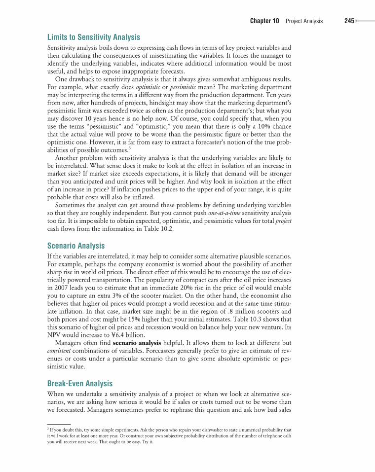
Scenario Analysis If the variables are interrelated, it may help to consider some alternative plausible scenarios. For example, perhaps the company economist is worried about the possibility of another sharp rise in world oil prices. The direct effect of this would be to encourage the use of elec-trically powered transportation. The popularity of compact cars after the oil price increases in 2007 leads you to estimate that an immediate 20% rise in the price of oil would enable you to capture an extra 3% of the scooter market. On the other hand, the economist also believes that higher oil prices would prompt a world recession and at the same time stimu-late inflation. In that case, market size might be in the region of .8 million scooters and both prices and cost might be 15% higher than your initial estimates. Table 10.3 shows that this scenario of higher oil prices and recession would on balance help your new venture. Its NPV would increase to ¥6.4 billion.

Managers often find scenario analysis helpful. It allows them to look at different but consistent combinations of variables. Forecasters generally prefer to give an estimate of rev-enues or costs under a particular scenario than to give some absolute optimistic or pes-simistic value.

Break-Even Analysis When we undertake a sensitivity analysis of a project or when we look at alternative sce-narios, we are asking how serious it would be if sales or costs turned out to be worse than we forecasted. Managers sometimes prefer to rephrase this question and ask how bad sales

3 If you doubt this, try some simple experiments. Ask the person who repairs your dishwasher to state a numerical probability that it will work for at least one more year. Or construct your own subjective probability distribution of the number of telephone calls you will receive next week. That ought to be easy. Try it.


confirming pages


can get before the project begins to lose money. This exercise is known as break-even analysis.

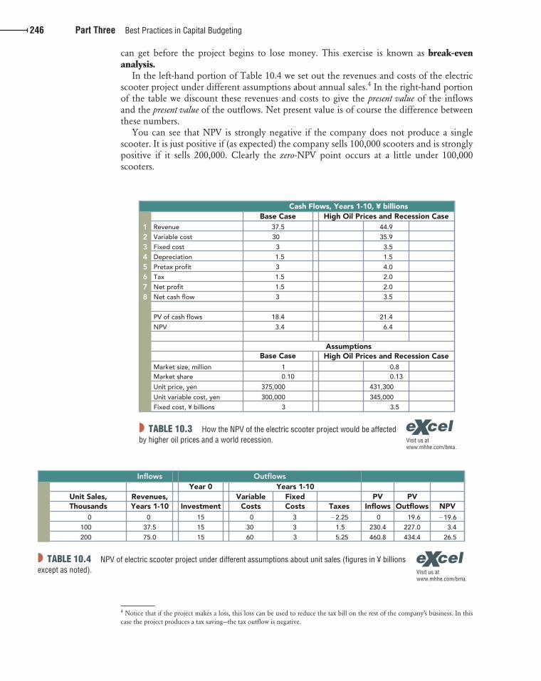
In the left-hand portion of Table 10.4 we set out the revenues and costs of the electric scooter project under different assumptions about annual sales. 4 In the right-hand portion of the table we discount these revenues and costs to give the present value of the inflows and the present value of the outflows. Net present value is of course the difference between these numbers.

You can see that NPV is strongly negative if the company does not produce a single scooter. It is just positive if (as expected) the company sells 100,000 scooters and is strongly positive if it sells 200,000. Clearly the zero -NPV point occurs at a little under 100,000 scooters.

4 Notice that if the project makes a loss, this loss can be used to reduce the tax bill on the rest of the company’s business. In this case the project produces a tax saving—the tax outflow is negative.

◗ TABLE 10.4 NPV of electric scooter project under different assumptions about unit sales (figures in ¥ billions except as noted). Visit us at

www.mhhe.com/bma.

Investment

Inflows Outflows

Unit Sales,Thousands

FixedCosts

VariableCosts Outflows

PVTaxes NPV

Year 0 Years 1-10Revenues,Years 1-10

0

37.5

75.0

15

15

15

0

30

60

3

3

3

�2.251.5

5.25

19.6

227.0

434.4

�19.63.4

26.5

0

100

200

PVInflows

0

230.4

460.8

◗ TABLE 10.3 How the NPV of the electric scooter project would be affected by higher oil prices and a world recession. Visit us at

www.mhhe.com/bma.

Revenue123456

Variable cost

Fixed cost

Depreciation

Pretax profit

Tax

7 Net profit

8 Net cash flow

PV of cash flows

NPV

Market size, millionMarket share

Unit price, yen

Unit variable cost, yenFixed cost, ¥ billions

Base Case

High Oil Prices and Recession Case

High Oil Prices and Recession Case

Base Case

Assumptions

Cash Flows, Years 1-10, ¥ billions

30

3

1.5

3

37.5

1.5

3

18.4

3.4

1.5

0.10

375,000

300,0003

1 0.80.13

431,300

345,0003.5

35.9

3.5

1.5

4.02.0

2.03.5

21.4

6.4

44.9


confirming pages


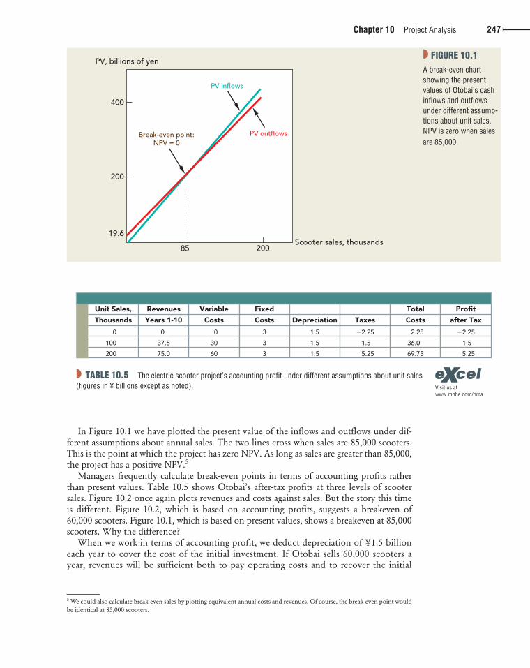
In Figure 10.1 we have plotted the present value of the inflows and outflows under dif-ferent assumptions about annual sales. The two lines cross when sales are 85,000 scooters. This is the point at which the project has zero NPV. As long as sales are greater than 85,000, the project has a positive NPV. 5

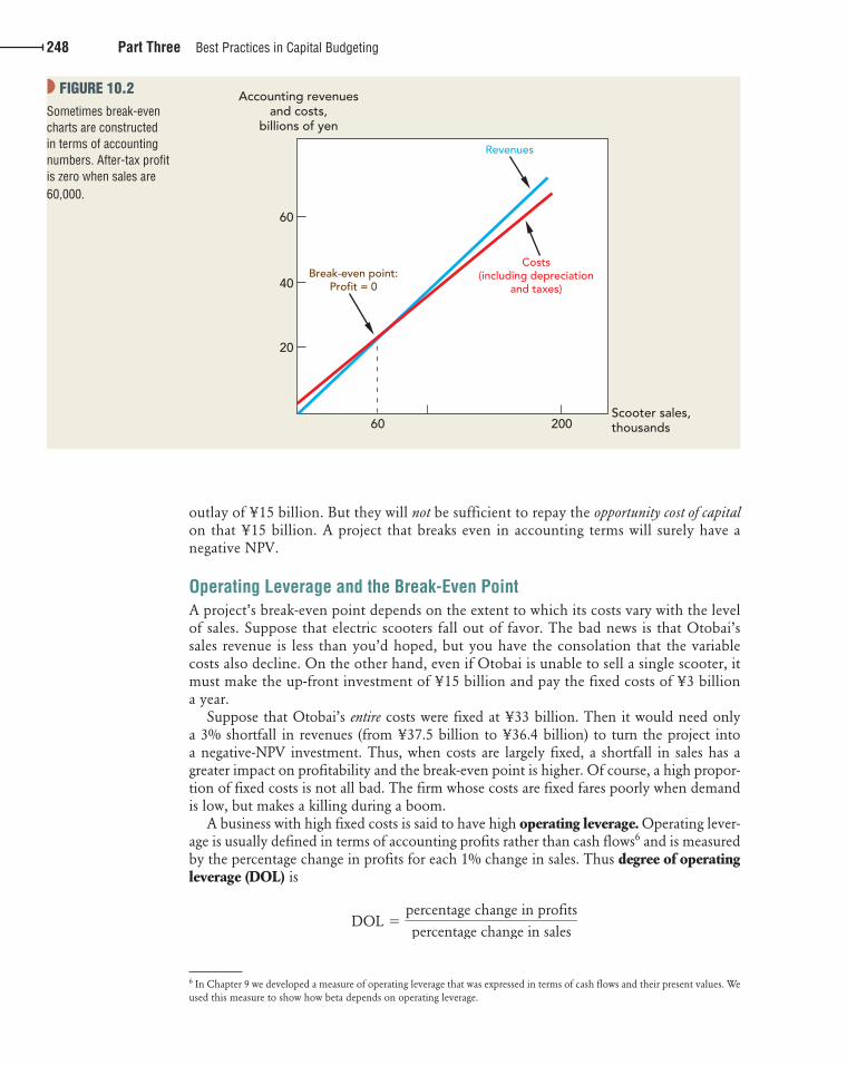
Managers frequently calculate break-even points in terms of accounting profits rather than present values. Table 10.5 shows Otobai’s after-tax profits at three levels of scooter sales. Figure 10.2 once again plots revenues and costs against sales. But the story this time is different. Figure 10.2 , which is based on accounting profits, suggests a breakeven of 60,000 scooters. Figure 10.1 , which is based on present values, shows a breakeven at 85,000 sc ooters. Why the difference?

When we work in terms of accounting profit, we deduct depreciation of ¥1.5 billion each year to cover the cost of the initial investment. If Otobai sells 60,000 scooters a year, revenues will be sufficient both to pay operating costs and to recover the initial

5 We could also calculate break-even sales by plotting equivalent annual costs and revenues. Of course, the break-even point would be identical at 85,000 scooters.

Scooter sales, thousands

Break-even point:NPV = 0

PV outflows

PV inflows

20085

PV, billions of yen

200

19.6

400

◗ FIGURE 10.1 A break-even chart showing the present values of Otobai’s cash inflows and outflows under different assump-tions about unit sales. NPV is zero when sales are 85,000.

◗ TABLE 10.5 The electric scooter project’s accounting profit under different assumptions about unit sales (figures in ¥ billions except as noted). Visit us at

www.mhhe.com/bma.

Unit Sales,

0

100

200

0

37.5

75.0

0

30

60

3

3

3

1.5

1.5

1.5

�2.25

1.5

5.25

2.25

36.0

69.75

�2.25

1.5

5.25

Thousands

Revenues

Years 1-10

Variable

Costs

Fixed

Costs Taxes

Total

Costs

Profit

after TaxDepreciation


confirming pages


outlay of ¥15 billion. But they will not be sufficient to repay the opportunity cost of capital on that ¥15 billion. A project that breaks even in accounting terms will surely have a negative NPV.

Operating Leverage and the Break-Even Point A project’s break-even point depends on the extent to which its costs vary with the level of sales. Suppose that electric scooters fall out of favor. The bad news is that Otobai’s sales revenue is less than you’d hoped, but you have the consolation that the variable costs also decline. On the other hand, even if Otobai is unable to sell a single scooter, it must make the up-front investment of ¥15 billion and pay the fixed costs of ¥3 billion a year.

Suppose that Otobai’s entire costs were fixed at ¥33 billion. Then it would need only a 3% shortfall in revenues (from ¥37.5 billion to ¥36.4 billion) to turn the project into a negative-NPV investment. Thus, when costs are largely fixed, a shortfall in sales has a greater impact on profitability and the break-even point is higher. Of course, a high propor-tion of fixed costs is not all bad. The firm whose costs are fixed fares poorly when demand is low, but makes a killing during a boom.

A business with high fixed costs is said to have high operating leverage. Operating lever-age is usually defined in terms of accounting profits rather than cash flows 6 and is measured by the percentage change in profits for each 1% change in sales. Thus degree of operating leverage (DOL) is

DOL 5percentage change in profits

percentage change in sales

6 In Chapter 9 we developed a measure of operating leverage that was expressed in terms of cash flows and their present values. We used this measure to show how beta depends on operating leverage.

Scooter sales,thousands

Break-even point:Profit = 0

Costs(including depreciation

and taxes)

Revenues

20060

Accounting revenuesand costs,

billions of yen

20

60

40

◗ FIGURE 10.2 Sometimes break-even charts are constructed in terms of accounting numbers. After-tax profit is zero when sales are 60,000.


confirming pages


The following simple formula 7 shows how DOL is related to the business’s fixed costs (including depreciation) as a proportion of pretax profits:

DOL 5 1 1fixed costs

profits

In the case of Otobai’s scooter project

DOL 5 1 113 1 1.5 2

35 2.5

A 1% shortfall in the scooter project’s revenues would result in a 2.5% shortfall in profits.

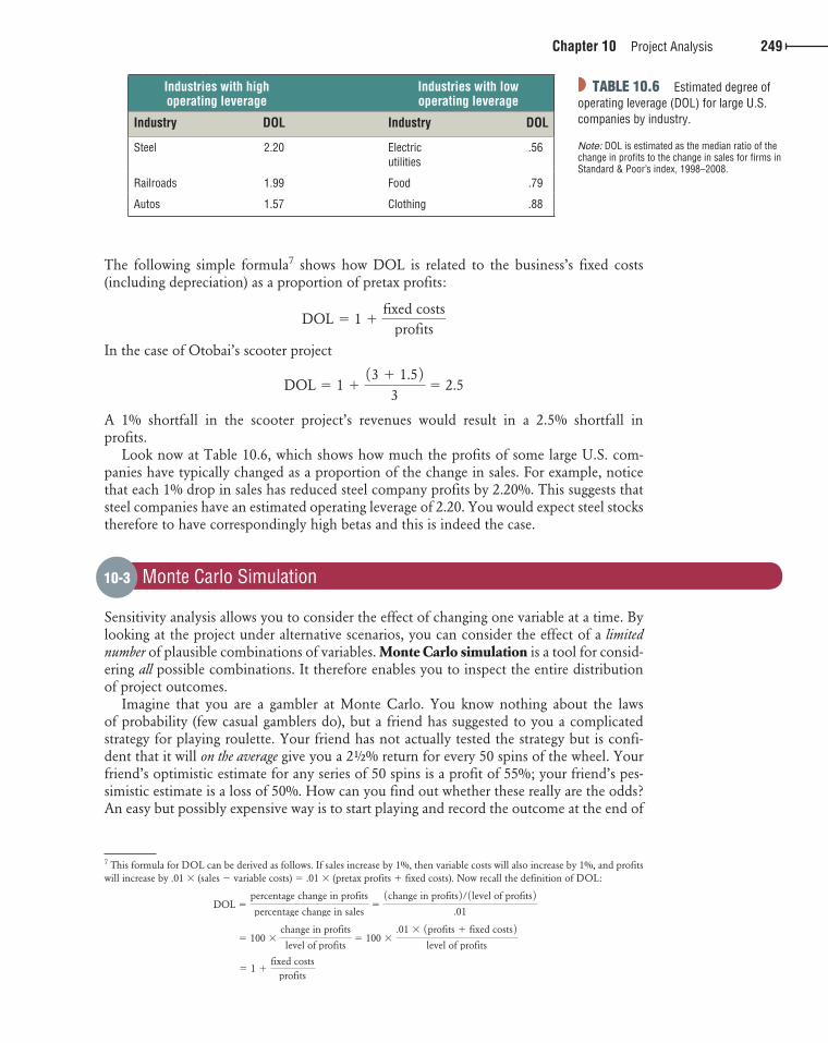
Look now at Table 10.6 , which shows how much the profits of some large U.S. com-panies have typically changed as a proportion of the change in sales. For example, notice that each 1% drop in sales has reduced steel company profits by 2.20%. This suggests that steel companies have an estimated operating leverage of 2.20. You would expect steel stocks therefore to have correspondingly high betas and this is indeed the case.

Sensitivity analysis allows you to consider the effect of changing one variable at a time. By looking at the project under alternative scenarios, you can consider the effect of a limited number of plausible combinations of variables. Monte Carlo simulation is a tool for consid-ering all possible combinations. It therefore enables you to inspect the entire distribution of project outcomes.

Imagine that you are a gambler at Monte Carlo. You know nothing about the laws of probability (few casual gamblers do), but a friend has suggested to you a complicated strategy for playing roulette. Your friend has not actually tested the strategy but is confi-dent that it will on the average give you a 2½% return for every 50 spins of the wheel. Your friend’s optimistic estimate for any series of 50 spins is a profit of 55%; your friend’s pes-simistic estimate is a loss of 50%. How can you find out whether these really are the odds? An easy but possibly expensive way is to start playing and record the outcome at the end of

7 This formula for DOL can be derived as follows. If sales increase by 1%, then variable costs will also increase by 1%, and profits will increase by .01 � (sales � variable costs) � .01 � (pretax profits � fixed costs). Now recall the definition of DOL:

DOL 5percentage change in profits

percentage change in sales51change in profits 2 / 1 level of profits 2

.01

5 100 3change in profits

level of profits5 100 3

.01 3 1profits 1 fixed costs 2

level of profits

5 1 1fixed costs

profits

10-3 Monte Carlo Simulation

◗ TABLE 10.6 Estimated degree of operating leverage (DOL) for large U.S. companies by industry.

Note: DOL is estimated as the median ratio of the change in profits to the change in sales for firms in Standard & Poor’s index, 1998–2008.

Industries with high operating leverage

Industries with low operating leverage

Industry DOL Industry DOL

Steel 2.20 Electric utilities

.56

Railroads 1.99 Food .79

Autos 1.57 Clothing .88


confirming pages


each series of 50 spins. After, say, 100 series of 50 spins each, plot a frequency distribution of the outcomes and calculate the average and upper and lower limits. If things look good, you can then get down to some serious gambling.

An alternative is to tell a computer to simulate the roulette wheel and the strategy. In other words, you could instruct the computer to draw numbers out of its hat to determine the outcome of each spin of the wheel and then to calculate how much you would make or lose from the particular gambling strategy.

That would be an example of Monte Carlo simulation. In capital budgeting we replace the gambling strategy with a model of the project, and the roulette wheel with a model of the world in which the project operates. Let us see how this might work with our project for an electrically powered scooter.

Simulating the Electric Scooter Project Step 1: Modeling the Project The first step in any simulation is to give the computer a precise model of the project. For example, the sensitivity analysis of the scooter project was based on the following implicit model of cash flow:

Cash flow 5 1 revenues 2 costs 2 depreciation 2 3 11 2 tax rate 2 1 depreciationRevenues 5 market size 3 market share 3 unit price

Costs 5 1market size 3 market share 3 variable unit cost 2 1 fixed cost

This model of the project was all that you needed for the simpleminded sensitivity analysis that we described above. But if you wish to simulate the whole project, you need to think about how the variables are interrelated.

For example, consider the first variable—market size. The marketing department has esti-mated a market size of 1 million scooters in the first year of the project’s life, but of course you do not know how things will work out. Actual market size will exceed or fall short of expectations by the amount of the department’s forecast error:

Market size, year 1 5 expected market size, year 1 3 11 1 forecast error, year 1 2

You expect the forecast error to be zero, but it could turn out to be positive or negative. Suppose, for example, that the actual market size turns out to be 1.1 million. That means a forecast error of 10%, or � .1:

Market size, year 1 5 1 3 11 1 .1 2 5 1.1 million

You can write the market size in the second year in exactly the same way:

Market size, year 2 5 expected market size, year 2 3 11 1 forecast error, year 2 2

But at this point you must consider how the expected market size in year 2 is affected by what happens in year 1. If scooter sales are below expectations in year 1, it is likely that they will continue to be below in subsequent years. Suppose that a shortfall in sales in year 1 would lead you to revise down your forecast of sales in year 2 by a like amount. Then

Expected market size, year 2 5 actual market size, year 1

Now you can rewrite the market size in year 2 in terms of the actual market size in the previous year plus a forecast error:

Market size, year 2 5 market size, year 1 3 11 1 forecast error, year 2 2

In the same way you can describe the expected market size in year 3 in terms of market size in year 2 and so on.


confirming pages


This set of equations illustrates how you can describe interdependence between differ-ent periods. But you also need to allow for interdependence between different variables. For example, the price of electrically powered scooters is likely to increase with market size. Suppose that this is the only uncertainty and that a 10% addition to market size would lead you to predict a 3% increase in price. Then you could model the first year’s price as follows:

Price, year 1 5 expected price, year 1 3 11 1 .3 3 error in market size forecast, year 1 2

Then, if variations in market size exert a permanent effect on price, you can define the second year’s price as

Price, year 2 5 expected price, year 2 3 11 1 .3 3 error in market size forecast, year 2 2 5 actual price, year 1 3 11 1 .3 3 error in market size forecast, year 2 2

Notice how we have linked each period’s selling price to the actual selling prices (including forecast error) in all previous periods. We used the same type of linkage for market size. These linkages mean that forecast errors accumulate; they do not cancel out over time. Thus, uncertainty increases with time: The farther out you look into the future, the more the actual price or market size may depart from your original forecast.

The complete model of your project would include a set of equations for each of the variables: market size, price, market share, unit variable cost, and fixed cost. Even if you allowed for only a few interdependencies between variables and across time, the result would be quite a complex list of equations. 8 Perhaps that is not a bad thing if it forces you to understand what the project is all about. Model building is like spinach: You may not like the taste, but it is good for you.

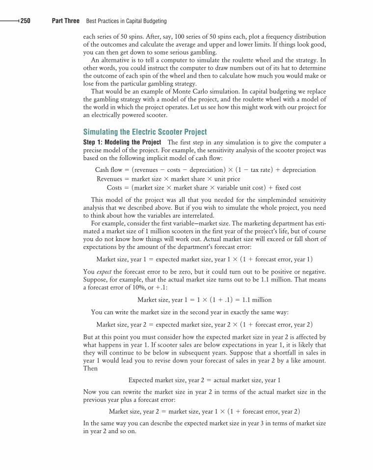
Step 2: Specifying Probabilities Remember the procedure for simulating the gambling strategy? The first step was to specify the strategy, the second was to specify the numbers on the roulette wheel, and the third was to tell the computer to select these numbers at random and calculate the results of the strategy:

Step 1Model the strategy

Step 2Specify numbers on

roulette wheel

Step 3Select numbers and

calculate resultsof strategy

The steps are just the same for your scooter project:

Step 1Model the project

Step 2Specify probabilitiesfor forecast errors

Step 3Select numbers forforecast errors andcalculate cash flows

Think about how you might go about specifying your possible errors in forecasting market size. You expect market size to be 1 million scooters. You obviously don’t think that you are underestimating or overestimating, so the expected forecast error is zero. On the other hand, the marketing department has given you a range of possible estimates. Market size could be as low as .85 million scooters or as high as 1.15 million scooters. Thus the forecast error has an expected value of 0 and a range of plus or minus 15%. If the marketing

8 Specifying the interdependencies is the hardest and most important part of a simulation. If all components of project cash flows were unrelated, simulation would rarely be necessary.


confirming pages


department has in fact given you the lowest and highest possible outcomes, actual market size should fall somewhere within this range with near certainty. 9

That takes care of market size; now you need to draw up similar estimates of the possible forecast errors for each of the other variables that are in your model.

Step 3: Simulate the Cash Flows The computer now samples from the distribution of the forecast errors, calculates the resulting cash flows for each period, and records them. After many iterations you begin to get accurate estimates of the probability distributions of the project cash flows—accurate, that is, only to the extent that your model and the probability distributions of the forecast errors are accurate. Remember the GIGO principle: “Garbage in, garbage out.”

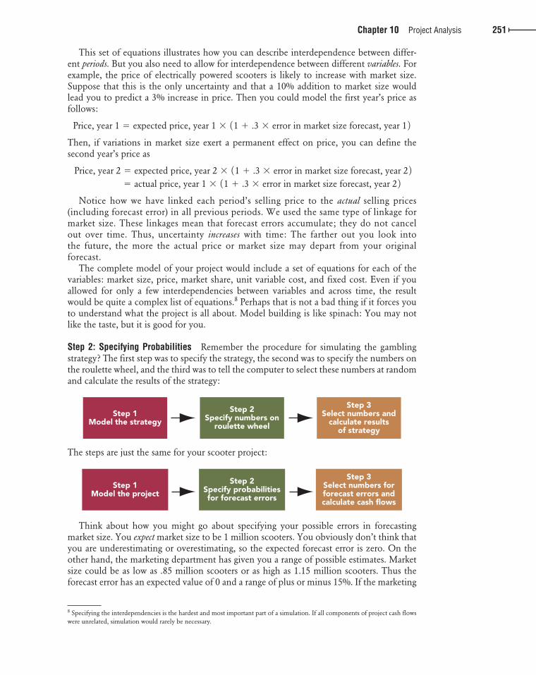
Figure 10.3 shows part of the output from an actual simulation of the electric scooter project. 10 Note the positive skewness of the outcomes—very large outcomes are more likely than very small ones. This is common when forecast errors accumulate over time. Because of the skewness the average cash flow is somewhat higher than the most likely outcome; in other words, a bit to the right of the peak of the distribution. 11

9 Suppose “near certainty” means “99% of the time.” If forecast errors are normally distributed, this degree of certainty requires a range of plus or minus three standard deviations.

Other distributions could, of course, be used. For example, the marketing department may view any market size between .85 and 1.15 million scooters as equally likely. In that case the simulation would require a uniform (rectangular) distribution of forecast errors. 10 These are actual outputs from Crystal Ball™ software. The simulation assumed annual forecast errors were normally distributed and ran through 10,000 trials. We thank Christopher Howe for running the simulation. An Excel program to simulate the Otobai project was kindly provided by Marek Jochec and is available on the Web site, www.mhhe.com/bma. 11 When you are working with cash-flow forecasts, bear in mind the distinction between the expected value and the most likely (or modal) value. Present values are based on expected cash flows—that is, the probability-weighted average of the possible future cash flows. If the distribution of possible outcomes is skewed to the right as in Figure 10.3 , the expected cash flow will be greater than the most likely cash flow.

Cash flow,billions of yen

Year 10: 10,000 Trials

8.5 9.08.07.57.06.56.05.55.04.54.03.53.02.52.01.51.0.50

Frequency.050

.000

.005

.010

.015

.020

.025

.030

.045

.040

.035

◗ FIGURE 10.3

Simulation of cash flows for year 10 of the electric scooter project.


confirming pages


Step 4: Calculate Present Value The distributions of project cash flows should allow you to calculate the expected cash flows more accurately. In the final step you need to discount these expected cash flows to find present value.

Simulation, though complicated, has the obvious merit of compelling the forecaster to face up to uncertainty and to interdependencies. Once you have set up your simulation model, it is a simple matter to analyze the principal sources of uncertainty in the cash flows and to see how much you could reduce this uncertainty by improving the forecasts of sales or costs. You may also be able to explore the effect of possible modifications to the project.

Simulation may sound like a panacea for the world’s ills, but, as usual, you pay for what you get. Sometimes you pay for more than you get. It is not just a matter of the time spent in building the model. It is extremely difficult to estimate interrelationships between vari-ables and the underlying probability distributions, even when you are trying to be honest. But in capital budgeting, forecasters are seldom completely impartial and the probability distributions on which simulations are based can be highly biased.

In practice, a simulation that attempts to be realistic will also be complex. Therefore the decision maker may delegate the task of constructing the model to management scientists or consultants. The danger here is that, even if the builders understand their creation, the decision maker cannot and therefore does not rely on it. This is a common but ironic experience.

When you use discounted cash flow (DCF) to value a project, you implicitly assume that the firm will hold the assets passively. But managers are not paid to be dummies. After they have invested in a new project, they do not simply sit back and watch the future unfold. If things go well, the project may be expanded; if they go badly, the project may be cut back or abandoned altogether. Projects that can be modified in these ways are more valuable than those that do not provide such flexibility. The more uncertain the outlook, the more valuable this flexibility becomes.

That sounds obvious, but notice that sensitivity analysis and Monte Carlo simulation do not recognize the opportunity to modify projects. 12 For example, think back to the Otobai electric scooter project. In real life, if things go wrong with the project, Otobai would aban-don to cut its losses. If so, the worst outcomes would not be as devastating as our sensitivity analysis and simulation suggested.

Options to modify projects are known as real options. Managers may not always use the term “real option” to describe these opportunities; for example, they may refer to “intangible advantages” of easy-to-modify projects. But when they review major investment proposals, these option intangibles are often the key to their decisions.

The Option to Expand Long-haul airfreight businesses such as FedEx need to move a massive amount of goods each day. Therefore, when Airbus announced delays to its A380 superjumbo freighter, FedEx turned to Boeing and ordered 15 of its 777 freighters to be delivered between 2009 and 2011. If business continues to expand, FedEx will need more aircraft. But rather than placing additional firm orders, the company secured a place in Boeing’s production line by acquiring options to buy a further 15 aircraft at a predetermined price. These options did not commit FedEx to expand but gave it the flexibility to do so.

12 Some simulation models do recognize the possibility of changing policy. For example, when a pharmaceutical company uses simulation to analyze its R&D decisions, it allows for the possibility that the company can abandon the development at each phase.

10-4 Real Options and Decision Trees


confirming pages


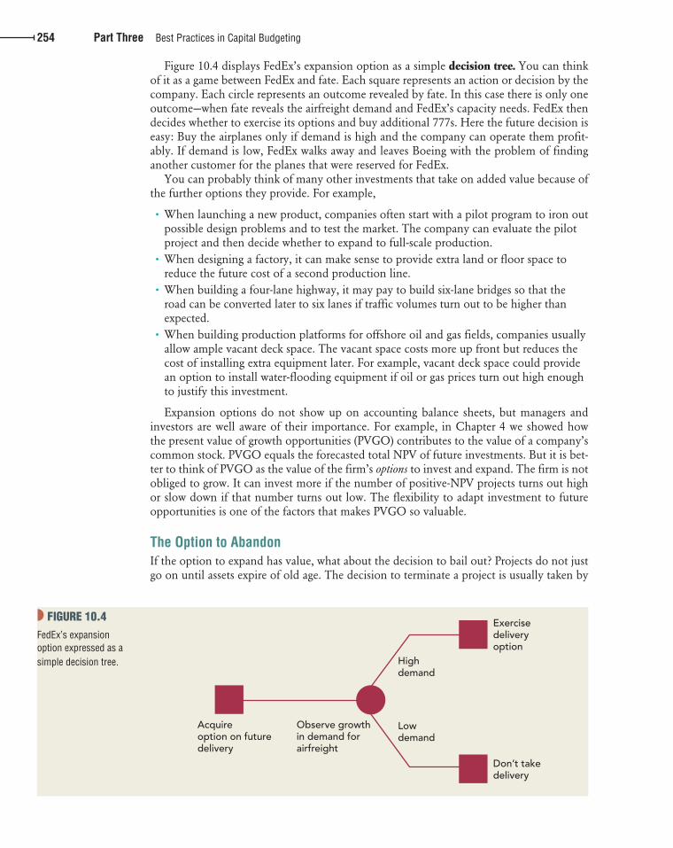
Figure 10.4 displays FedEx’s expansion option as a simple decision tree. You can think of it as a game between FedEx and fate. Each square represents an action or decision by the company. Each circle represents an outcome revealed by fate. In this case there is only one outcome—when fate reveals the airfreight demand and FedEx’s capacity needs. FedEx then decides whether to exercise its options and buy additional 777s. Here the future decision is easy: Buy the airplanes only if demand is high and the company can operate them profit-ably. If demand is low, FedEx walks away and leaves Boeing with the problem of finding another customer for the planes that were reserved for FedEx.

You can probably think of many other investments that take on added value because of the further options they provide. For example,

• When launching a new product, companies often start with a pilot program to iron out possible design problems and to test the market. The company can evaluate the pilot project and then decide whether to expand to full-scale production.

• When designing a factory, it can make sense to provide extra land or floor space to reduce the future cost of a second production line.

• When building a four-lane highway, it may pay to build six-lane bridges so that the road can be converted later to six lanes if traffic volumes turn out to be higher than expected.

• When building production platforms for offshore oil and gas fields, companies usually allow ample vacant deck space. The vacant space costs more up front but reduces the cost of installing extra equipment later. For example, vacant deck space could provide an option to install water-flooding equipment if oil or gas prices turn out high enough to justify this investment.

Expansion options do not show up on accounting balance sheets, but managers and investors are well aware of their importance. For example, in Chapter 4 we showed how the present value of growth opportunities (PVGO) contributes to the value of a company’s common stock. PVGO equals the forecasted total NPV of future investments. But it is bet-ter to think of PVGO as the value of the firm’s options to invest and expand. The firm is not obliged to grow. It can invest more if the number of positive-NPV projects turns out high or slow down if that number turns out low. The flexibility to adapt investment to future opportunities is one of the factors that makes PVGO so valuable.

The Option to Abandon If the option to expand has value, what about the decision to bail out? Projects do not just go on until assets expire of old age. The decision to terminate a project is usually taken by

◗ FIGURE 10.4 FedEx’s expansion option expressed as a simple decision tree. High

demand

Observe growthin demand forairfreight

Acquireoption on futuredelivery

Exercisedeliveryoption

Don’t takedelivery

Lowdemand


confirming pages


management, not by nature. Once the project is no longer profitable, the company will cut its losses and exercise its option to abandon the project.

Some assets are easier to bail out of than others. Tangible assets are usually easier to sell than intangible ones. It helps to have active secondhand markets, which really exist only for stan-dardized items. Real estate, airplanes, trucks, and certain machine tools are likely to be relatively easy to sell. On the other hand, the knowledge accumulated by a software company’s research and development program is a specialized intangible asset and probably would not have signifi-cant abandonment value. (Some assets, such as old mattresses, even have negative abandonment value; you have to pay to get rid of them. It is costly to decommission nuclear power plants or to reclaim land that has been strip-mined.)

● ● ● ● ●

EXAMPLE 10.1 ● Bailing Out of the Outboard-Engine Project

Managers should recognize the option to abandon when they make the initial investment in a new project or venture. For example, suppose you must choose between two technolo-gies for production of a Wankel-engine outboard motor.

1. Technology A uses computer-controlled machinery custom-designed to produce the complex shapes required for Wankel engines in high volumes and at low cost. But if the Wankel outboard does not sell, this equipment will be worthless.

2. Technology B uses standard machine tools. Labor costs are much higher, but the machinery can be sold for $17 million if demand turns out to be low.

Just for simplicity, assume that the initial capital outlays are the same for both technolo-gies. If demand in the first year is buoyant, technology A will provide a payoff of $24 mil-lion. If demand is sluggish, the payoff from A is $16 million. Think of these payoffs as the project’s cash flow in the first year of production plus the value in year 1 of all future cash flows. The corresponding payoffs to technology B are $22.5 million and $15 million:

Payoffs from Producing Outboard ($ millions)

Technology A Technology B

Buoyant demand $24.0 $22.5

Sluggish demand 16.0 15.0*

* Composed of a cash flow of $1.5 million and a PV in year 1 of 13.5 million.

Technology A looks better in a DCF analysis of the new product because it was designed to have the lowest possible cost at the planned production volume. Yet you can sense the advantage of the flexibility provided by technology B if you are unsure whether the new outboard will sink or swim in the marketplace. If you adopt technology B and the outboard is not a success, you are better off collecting the first year’s cash flow of $1.5 million and then selling the plant and equipment for $17 million.

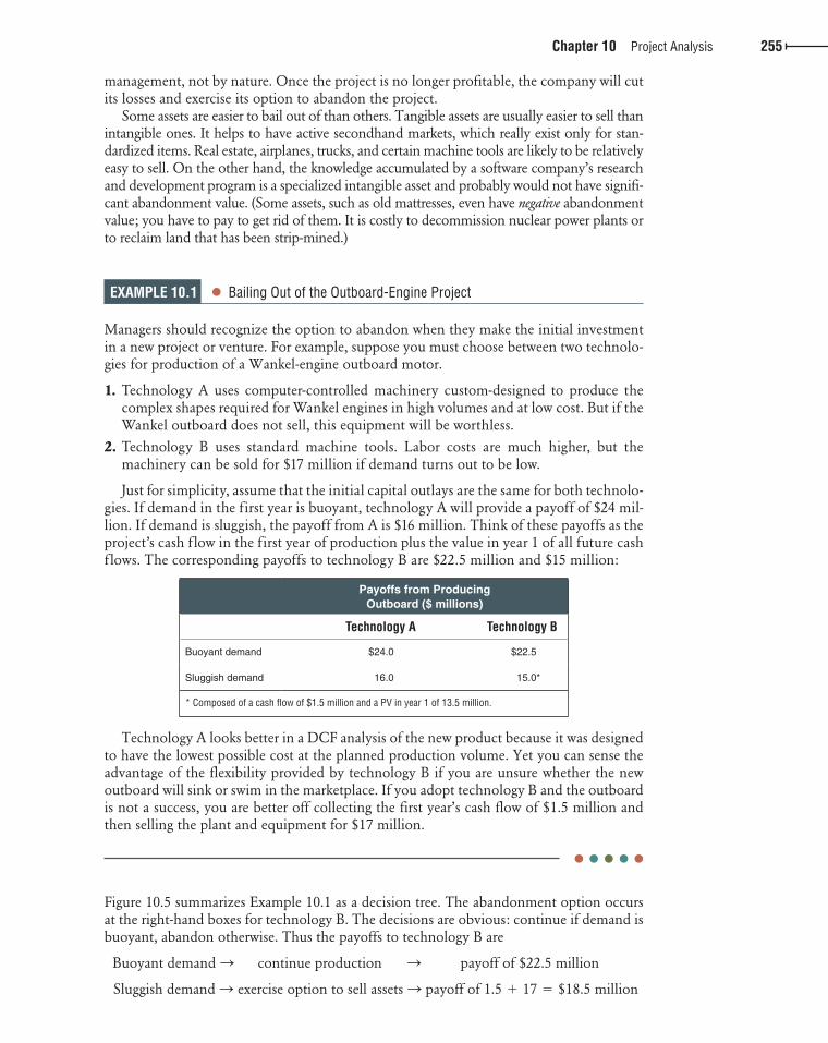
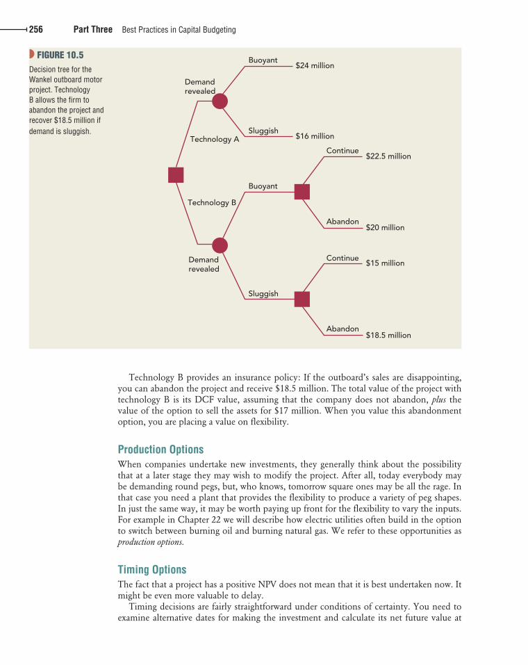
Figure 10.5 summarizes Example 10.1 as a decision tree. The abandonment option occurs at the right-hand boxes for technology B. The decisions are obvious: continue if demand is buoyant, abandon otherwise. Thus the payoffs to technology B are

Buoyant demand S continue production S payoff of $22.5 million

Sluggish demand S exercise option to sell assets S payoff of 1.5 1 17 5 $18.5 million


confirming pages


Technology B provides an insurance policy: If the outboard’s sales are disappointing, you can abandon the project and receive $18.5 million. The total value of the project with technology B is its DCF value, assuming that the company does not abandon, plus the value of the option to sell the assets for $17 million. When you value this abandonment option, you are placing a value on flexibility.

Production Options When companies undertake new investments, they generally think about the possibility that at a later stage they may wish to modify the project. After all, today everybody may be demanding round pegs, but, who knows, tomorrow square ones may be all the rage. In that case you need a plant that provides the flexibility to produce a variety of peg shapes. In just the same way, it may be worth paying up front for the flexibility to vary the inputs. For example in Chapter 22 we will describe how electric utilities often build in the option to switch between burning oil and burning natural gas. We refer to these opportunities as production options.

Timing Options The fact that a project has a positive NPV does not mean that it is best undertaken now. It might be even more valuable to delay.

Timing decisions are fairly straightforward under conditions of certainty. You need to examine alternative dates for making the investment and calculate its net future value at

Technology A

Demandrevealed

Demandrevealed

Technology B

Buoyant

Sluggish

$24 million

$16 million

$22.5 million

$20 million

$15 million

$18.5 million

Abandon

Continue

Continue

Abandon

Buoyant

Sluggish

◗ FIGURE 10.5 Decision tree for the Wankel outboard motor project. Technology B allows the firm to abandon the project and recover $18.5 million if demand is sluggish.


confirming pages


each of these dates. Then, to find which of the alternatives would add most to the firm’s current value, you must discount these net future values back to the present:

Net present value of investment if undertaken at time t 5Net future value at date t

11 1 r 2 t

The optimal date to undertake the investment is the one that maximizes its contribution to the value of your firm today. This procedure should already be familiar to you from Chapter 6, where we worked out when it was best to cut a tract of timber.

In the timber-cutting example we assumed that there was no uncertainty about the cash flows, so that you knew the optimal time to exercise your option. When there is uncertainty, the timing option is much more complicated. An opportunity not taken at t � 0 might be more or less attractive at t � 1; there is rarely any way of knowing for sure. Perhaps it is better to strike while the iron is hot even if there is a chance that it will become hotter. On the other hand, if you wait a bit you might obtain more information and avoid a bad mistake. That is why you often find that managers choose not to invest today in projects where the NPV is only marginally positive and there is much to be learned by delay.

More on Decision Trees We will return to all these real options in Chapter 22, after we have covered the theory of option valuation in Chapters 20 and 21. But we will end this chapter with a closer look at decision trees.

Decision trees are commonly used to describe the real options imbedded in capital investment projects. But decision trees were used in the analysis of projects years before real options were first explicitly identified. Decision trees can help to understand project risk and how future decisions will affect project cash flows. Even if you never learn or use option valuation theory, decision trees belong in your financial toolkit.

The best way to appreciate how decision trees can be used in project analysis is to work through a detailed example.

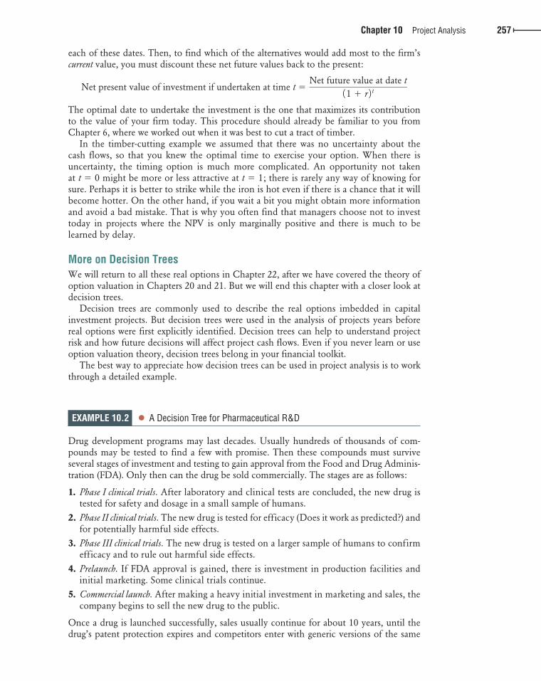
EXAMPLE 10.2 ● A Decision Tree for Pharmaceutical R&D

Drug development programs may last decades. Usually hundreds of thousands of com-pounds may be tested to find a few with promise. Then these compounds must survive several stages of investment and testing to gain approval from the Food and Drug Adminis-tration (FDA). Only then can the drug be sold commercially. The stages are as follows:

1. Phase I clinical trials. After laboratory and clinical tests are concluded, the new drug is tested for safety and dosage in a small sample of humans.

2. Phase II clinical trials. The new drug is tested for efficacy (Does it work as predicted?) and for potentially harmful side effects.

3. Phase III clinical trials. The new drug is tested on a larger sample of humans to confirm efficacy and to rule out harmful side effects.

4. Prelaunch. If FDA approval is gained, there is investment in production facilities and initial marketing. Some clinical trials continue.

5. Commercial launch. After making a heavy initial investment in marketing and sales, the company begins to sell the new drug to the public.

Once a drug is launched successfully, sales usually continue for about 10 years, until the drug’s patent protection expires and competitors enter with generic versions of the same


confirming pages


chemical compound. The drug may continue to be sold off-patent, but sales volume and profits are much lower.

The commercial success of FDA-approved drugs varies enormously. The PV of a “block-buster” drug at launch can be 5 or 10 times the PV of an average drug. A few blockbusters can generate most of a large pharmaceutical company’s profits. 13

No company hesitates to invest in R&D for a drug that it knows will be a blockbuster. But the company will not find out for sure until after launch. Sometimes a company thinks it has a blockbuster, only to discover that a competitor has launched a better drug first.

Sometimes the FDA approves a drug but limits its scope of use. Some drugs, though effective, can only be prescribed for limited classes of patients; other drugs can be pre-scribed much more widely. Thus the manager of a pharmaceutical R&D program has to assess the odds of clinical success and the odds of commercial success. A new drug may be abandoned if it fails clinical trials—for example, because of dangerous side effects—or if the outlook for profits is discouraging.

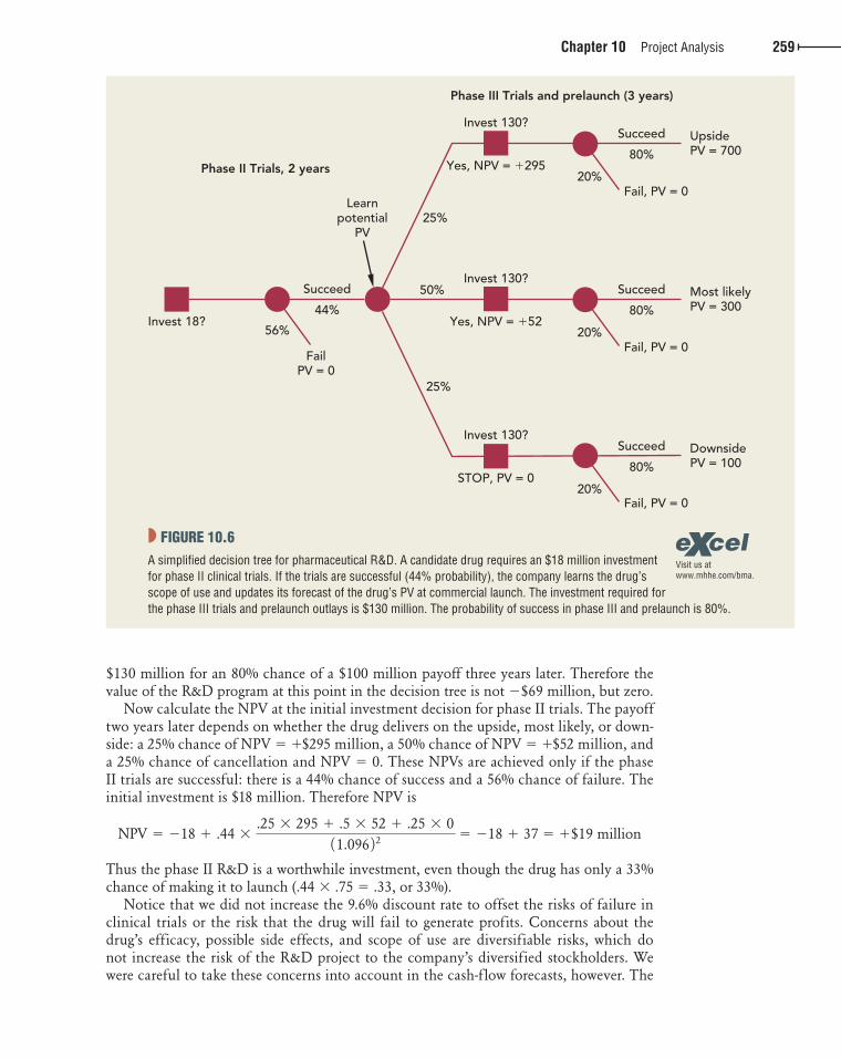
Figure 10.6 is a decision tree that illustrates these decisions. We have assumed that a new drug has passed phase I clinical trials with flying colors. Now it requires an invest-ment of $18 million for phase II trials. These trials take two years. The probability of success is 44%.13

If the trials are successful, the manager learns the commercial potential of the drug, which depends on how widely it can be used. Suppose that the forecasted PV at launch depends on the scope of use allowed by the FDA. These PVs are shown at the far right of the decision tree: an upside outcome of NPV � $700 million if the drug can be widely used, a most likely case with NPV � $300 million, and a downside case of NPV � $100 million if the drug’s scope is greatly restricted. 14 The NPVs are the payoffs at launch after investment in marketing. Launch comes three years after the start of phase III if the drug is approved by the FDA. The probabilities of the upside, most likely, and downside outcomes are 25%, 50%, and 25%, respectively.

A further R&D investment of $130 million is required for phase III trials and for the prelaunch period. (We have combined phase III and prelaunch for simplicity.) The prob-ability of FDA approval and launch is 80%.

Now let’s value the investments in Figure 10.6 . We assume a risk-free rate of 4% and market risk premium of 7%. If FDA-approved pharmaceutical products have asset betas of .8, the opportunity cost of capital is 4 � .8 � 7 � 9.6%.

We work back through the tree from right to left. The NPVs at the start of phase III trials are:

NPV 1upside 2 5 2130 1 .8 370011.096 2 3

5 1$295 million

NPV 1most likely 2 5 2130 1 .8 330011.096 2 3

5 1$52 million

NPV 1downside 2 5 2130 1 .8 310011.096 2 3

5 2$69 million

Since the downside NPV is negative at �$69 million, the $130 million investment at the start of phase III should not be made in the downside case. There is no point investing

13 The Web site of the Tufts Center for the Study of Drug Development ( http://csdd.tufts.edu ) provides a wealth of information about the costs and risks of pharmaceutical R&D. 14 The most likely case is not the average outcome, because PVs in the pharmaceutical business are skewed to the upside. The aver-age PV is .25 � 700 � .5 � 300 � .25 � 100 � $350 million.


confirming pages


$130 million for an 80% chance of a $100 million payoff three years later. Therefore the value of the R&D program at this point in the decision tree is not �$69 million, but zero.

Now calculate the NPV at the initial investment decision for phase II trials. The payoff two years later depends on whether the drug delivers on the upside, most likely, or down-side: a 25% chance of NPV � � $295 million, a 50% chance of NPV � � $52 million, and a 25% chance of cancellation and NPV � 0. These NPVs are achieved only if the phase II trials are successful: there is a 44% chance of success and a 56% chance of failure. The initial investment is $18 million. Therefore NPV is

NPV 5 218 1 .44 3.25 3 295 1 .5 3 52 1 .25 3 0

11.096 2 25 218 1 37 5 1$19 million

Thus the phase II R&D is a worthwhile investment, even though the drug has only a 33% chance of making it to launch (.44 � .75 � .33, or 33%).

Notice that we did not increase the 9.6% discount rate to offset the risks of failure in clinical trials or the risk that the drug will fail to generate profits. Concerns about the drug’s efficacy, possible side effects, and scope of use are diversifiable risks, which do not increase the risk of the R&D project to the company’s diversified stockholders. We were careful to take these concerns into account in the cash-flow forecasts, however. The

FailPV = 0

Succeed

Learnpotential

PV

Phase II Trials, 2 years

Phase III Trials and prelaunch (3 years)

44%

56%Invest 18?

Fail, PV = 0

UpsidePV = 700

Invest 130?

Yes, NPV = �295

Succeed

80%

20%

Most likelyPV = 300

Invest 130?

Yes, NPV = �52

Succeed

80%

20%

25%

50%

25%

DownsidePV = 100

Invest 130?

STOP, PV = 0

Succeed

80%

20%

Fail, PV = 0

Fail, PV = 0

◗ FIGURE 10.6 A simplified decision tree for pharmaceutical R&D. A candidate drug requires an $18 million investment for phase II clinical trials. If the trials are successful (44% probability), the company learns the drug’s scope of use and updates its forecast of the drug’s PV at commercial launch. The investment required for the phase III trials and prelaunch outlays is $130 million. The probability of success in phase III and prelaunch is 80%.



Visi

t us

at w

ww

.mhh

e.co

m/b

ma

confirming pages


decision tree in Figure 10.6 keeps track of the probabilities of success or failure and the probabilities of upside and downside outcomes. 15

Figures 10.5 and 10.6 are both examples of abandonment options. We have not explic-itly modeled the investments as options, however, so our NPV calculation is incomplete. We show how to value abandonment options in Chapter 22.

Pro and Con Decision Trees Any cash-flow forecast rests on some assumption about the firm’s future investment and oper-ating strategy. Often that assumption is implicit. Decision trees force the underlying strategy into the open. By displaying the links between today’s decisions and tomorrow’s decisions, they help the financial manager to find the strategy with the highest net present value.

The decision tree in Figure 10.6 is a simplified version of reality. For example, you could expand the tree to include a wider range of NPVs at launch, possibly including some chance of a blockbuster or of intermediate outcomes. You could allow information about the NPVs to arrive gradually, rather than just at the start of phase III. You could introduce the investment decision at phase I trials and separate the phase III and prelaunch stages. You may wish to draw a new decision tree covering these events and decisions. You will see how fast the circles, squares, and branches accumulate.

The trouble with decision trees is that they get so ________ complex so ________ quickly (insert your own expletives). Life is complex, however, and there is very little we can do about it. It is therefore unfair to criticize decision trees because they can become complex. Our criticism is reserved for analysts who let the complexity become overwhelming. The point of decision trees is to allow explicit analysis of possible future events and decisions. They should be judged not on their comprehensiveness but on whether they show the most important links between today’s and tomorrow’s decisions. Decision trees used in real life will be more complex than Figure 10.6 , but they will nevertheless display only a small fraction of possible future events and decisions. Decision trees are like grapevines: They are productive only if they are vigorously pruned.

15 The market risk attaching to the PVs at launch is recognized in the 9.6% discount rate.

● ● ● ● ●

Earlier chapters explained how companies calculate a project’s NPV by forecasting the cash flows and discounting them at a rate that reflects project risk. The end result is the project’s contribution to shareholder wealth. Understanding discounted-cash-flow analysis is important, but there is more to good capital budgeting practice than an ability to discount.

First, companies need to establish a set of capital budgeting procedures to ensure that deci-sions are made in an orderly manner. Most companies prepare an annual capital budget, which is a list of investment projects planned for the coming year. Inclusion of a project in the capital budget does not constitute final approval for the expenditure. Before the plant or division can go ahead with a proposal, it will usually need to submit an appropriation request that includes detailed forecasts, a discounted-cash-flow analysis, and back-up information.

Sponsors of capital investment projects are tempted to overstate future cash flows and under-state risks. Therefore firms need to encourage honest and open discussion. They also need pro-cedures to ensure that projects fit in with the company’s strategic plans and are developed on a consistent basis. (These procedures should not include fudge factors added to project hurdle rates in an attempt to offset optimistic forecasts.) Later, after a project has begun to operate, the firm can follow up with a postaudit. Postaudits identify problems that need fixing and help the firm learn from its mistakes.

SUMMARY

● ● ● ● ●


Documents

Project Analysis - kuswanto.staff.gunadarma.ac.idkuswanto.staff.gunadarma.ac.id/Downloads/files/60502/CHAPTER-10.pdf · and maybe some further work on the test bed would confirm the