Embed Size (px)
Citation preview
RAND Journal of EconomicsVol. 00, No. 0, xxx 2014pp. 1–26
Project design with limited commitmentand teams
George Georgiadis∗Steven A. Lippman∗∗and
Christopher S. Tang∗∗
We study the interaction between a group of agents who exert effort to complete a project and amanager who chooses its objectives. The manager has limited commitment power so that she cancommit to the objectives only when the project is sufficiently close to completion. We show that themanager has incentives to extend the project as it progresses. This result has two implications.First, the manager will choose a larger project if she has less commitment power. Second, themanager should delegate the decision rights over the project size to the agents unless she hassufficient commitment power.
1. Introduction
� A key component of a project, such as the development of a new product, is choosing thefeatures that must be included before the decision maker deems the product ready to market.Naturally, which features should be included must be communicated to the relevant stakeholders.When choosing these features, the decision maker must balance the added value derived froma bigger or a more complex project (i.e., one that contains more features) against the additionalcost associated with designing and implementing the additional features. Such costs include notonly engineering inputs but also the implicit cost associated with delayed cash flow.
An intrinsic challenge involved in choosing the requirements of a project is that the managermay not be able to commit to them in advance. This can be due to the fact that the requirements aredifficult to describe; for example, if the project involves significant novelty in quality or design.What we have in mind about the incontractibility of the project requirements was eloquentlyposed by Tirole (1999):
∗ California Institute of Technology and Boston University; [email protected].∗∗ UCLA; [email protected], [email protected] are grateful to the coeditor, David Martimont, to two anonymous referees, Simon Board, Alessandro Bonatti, RickBrenner, Florian Ederer, Hugo Hopenhayn, John Ledyard, Fei Li, Moritz Meyer-Ter-Vehn, Stephen Morris, ThomasPalfrey, Michael Riordan, as well as seminar participants at Caltech, Cambridge University, London Business School,Stanford University, UCLA, the 2013 Annual IO Theory Conference in Durham, NC, and the 2013 North AmericanSummer Meetings of the Econometric Society in Los Angeles, CA.
Copyright C© 2014, RAND. 1

2 / THE RAND JOURNAL OF ECONOMICS
In practice, the parties are unlikely to be able to describe precisely the specifics of aninnovation in an ex ante contract, given that the research process is precisely concernedwith finding out these specifics, although they are able to describe it ex post.
In addition, committing to specific requirements may be difficult due to an asymmetry in thebargaining power of the parties involved. For example, if the project is undertaken in-housewhere the manager can significantly influence the team members’ career paths and contracts aretypically implicit, then the manager will tend to be less able to commit relative to the case inwhich the project is outsourced and contracts are explicit.
A fitting example stems from the development of Apple’s first generation iPod. Anecdotalevidence indicates that Steve Jobs kept changing the requirements of the iPod as the projectprogressed. In particular, the development team would get orders such as, “Steve doesn’t think itis loud enough,” or “the sharps are not sharp enough,” or “the menu is not coming up fast enough”(Wired Magazine, 2004). This suggests that committing to a set of features and requirements earlyon was not desirable in the development of an innovative new product such as the iPod back in2001.
Similarly, consider a design project, such as the process of designing a new automobile. Ifthe decision maker were able to provide a precise description of the design for it to be approvedat the outset of the process, then there would be no need to undertake it in the first place. Inpractice, the decision maker must guide the design team as the final product takes shape to fulfillher objectives.
Finally, changing the requirements of a project (often referred to as moving the goal post) iscommon in project management (Brenner, 2001). One prominent example is Boeing’s 787 Dream-liner project. The original set of project goals was to develop a lightweight, fuel-efficient aircraftthat would meet the customers’ needs for lower operating costs. On top of these original projectgoals, Boeing’s senior management then decided to outsource parts of the design, engineering,and manufacturing processes to some 50 external “strategic partners” to reduce developmentcosts and time. From the perspective of Boeing’s engineers, a new goal was appended to theoriginal set of project goals: restructure the design and manufacturing processes by overseeingand coordinating the work performed by internal engineers and those external strategic partners(Brenner, 2013). In addition, Boeing sought to maximize the usage of composite materials toreduce the weight of the 787 aircraft. However, due to unproven technology, Boeing’s engineerswere unable to provide accurate specifications at the outset of the project without the risk ofcompromising the intended performance and safety standards. Indeed, it was only in 2009, afterexamining the results of a series of fatigue and stress tests, that Boeing finally committed to theamount of composite materials to be used on the 787 aircraft (Tang and Zimmerman, 2009).
In this article, we propose a parsimonious model to analyze a dynamic contribution game inwhich a group of agents collaborate to complete a project. The project progresses at a rate thatdepends on the agents’ costly effort, and it generates a payoff upon completion. Formally, the stateof the project qt starts at 0, and it progresses according to dqt = ∑n
i=1 ai,t dt , where ai,t denotesthe effort level of agent i at time t . The project generates a payoff at the first stopping time τ suchthat qτ = Q, where Q is a one-dimensional parameter that captures the project requirements,or equivalently, the project size. The manager is the residual claimant of the project, and shepossesses the decision rights over its size. It is noteworthy that the model is very tractable, andpayoffs and strategies are derived in closed-form.
In Section 3 we analyze the agents’ problem given a fixed project size. We characterizethe (essentially) unique Markov Perfect Equilibrium (MPE), wherein at every moment, eachagent’s strategy depends solely on the current state of the project. In addition, we characterize acontinuum of (non-Markovian) Public Perfect Equilibria (PPE), in which along the equilibriumpath, the agents choose their effort by maximizing a convex combination of their individual andthe team’s discounted payoff. Motivated by the concepts of insiders and outsiders (who act in thebest interest of the team and in their own best interest, respectively) introduced by Akerlof and
C© RAND 2014.

GEORGIADIS, LIPPMAN, AND TANG / 3
Kranton (2000), the weight that agents place on maximizing the team’s payoff can be interpretedas a measure of the team’s cooperativeness. A key result is that the agents exert greater effortthe closer the project is to completion. Intuitively, this is because they discount time and arecompensated upon completion, so that their incentives become stronger as the project progresses.
In Section 4 we analyze the manager’s problem and determine her optimal project size.Her fundamental trade-off is that a larger project generates a bigger payoff upon completion butrequires more effort (and hence takes longer) to be completed. To model the manager’s limitedability to commit, we assume that given the current state of the project qt , she can commit toany Q ∈ [qt , qt + y], where y ≥ 0 captures the commitment power. Therefore, the manager cancommit to a project size Q > y only after the agents have made sufficient progress such thatqt ≥ Q − y.
For example, y will tend to be larger in a construction project, where the requirements aretypically standardized and easy to define, than in a project that involves a significant innovationor quality component, where the requirements of the final output cannot be contracted on untilthe project is at a sufficiently advanced stage. Similarly, y will typically be small in design-relatedprojects such as automotive design, as the requirements are difficult to describe. If the projectis outsourced and contracts are explicit, then y will tend to be larger than the case in which itis undertaken in-house, where the manager can influence the team members’ career paths andcontracts are typically implicit.
The main result is that the manager’s incentives propel her to extend the project as itprogresses; for example, by introducing additional requirements. The manager chooses the projectsize by trading off the marginal benefit of a larger project against the marginal cost associatedwith a longer wait until the larger project is completed. However, as the project progresses,the agents increase their effort, so that this marginal cost decreases, whereas the respectivemarginal benefit does not change. As the project size will be chosen such that the two marginalvalues are equal, it follows that the manager’s optimal project size increases as the projectprogresses.
An implication of this result is that the manager’s optimal project size decreases in hercommitment power. If the manager has sufficiently large commitment power, then she willcommit to her optimal project size at time 0. Otherwise, she can commit to a smaller thanideal project at time 0, or she must wait until the project is at a sufficiently advanced stage sothat she can commit to her optimal project size then. However, once such an advanced stagehas been reached, her optimal project size is larger than it was originally, and the managerfaces the same dilemma as at time 0. Nevertheless, we show that the manager always prefersto wait, and as a consequence, she will choose a bigger project the smaller her commitmentpower.
Anticipating that the manager will choose a larger project if she has less commitment power,the agents decrease their effort, which renders the manager worse off. To mitigate her commitmentproblem, assuming that the agents receive a share of the project’s worth upon completion (i.e.,an equity contract), the manager might delegate the decision rights over the project size to them.In this case, the agents will choose a smaller project than is optimal for the manager, but theirpreferences are time-consistent. Intuitively, because (unlike the manager) they also trade offthe cost of effort when choosing the project size, their marginal cost associated with a largerproject does not decrease as the project progresses. As a result, the manager’s discounted profit isindependent of the commitment power under delegation, whereas it increases in her commitmentpower when she retains the decision rights over the project size. We show that there exists aninterior threshold such that delegation is optimal unless the manager has sufficient commitmentpower.
� Related literature. First and foremost, this article is related to the literature on dynamiccontribution games. The general theme of these games is that a group of agents interact repeatedly,and in every period (or moment), each agent chooses his contribution (or effort) to a joint project
C© RAND 2014.
4 / THE RAND JOURNAL OF ECONOMICS
at a private cost. Contributions accumulate until they reach a certain threshold, at which pointthe game ends. Agents receive flow payoffs while the game is in progress, a lump-sum payoffat the end, or a combination thereof. Admati and Perry (1991) and Marx and Matthews (2000)show that contributing little by little over multiple periods, each conditional on the previouscontributions of the other agents, helps mitigate the free-rider problem. More recently, Yildirim(2006) and Kessing (2007) show that in contrast to the case in which the project generates flowpayments while it is in progress, as studied by Fershtman and Nitzan (1991), efforts are strategiccomplements when the agents receive a payoff only upon completion. Georgiadis (2013) studieshow the incentives to contribute to a public good project depend on the team composition andexamines how a manager should choose the team composition and the agents’ compensationscheme. A feature common to most articles in this literature is that the size of the project isgiven exogenously. However, in applications (e.g., new product development), the choice of theobjectives of any given project is typically a central decision that must be made. Our contributionto this literature is to propose a tractable model to study this family of dynamic contributiongames, to endogenize the size of the project, and to examine how the optimal project size dependson who has the decision rights and on the magnitude of the decision maker’s commitmentpower.
A second strand of related literature is that on incomplete contracting. In particular, ourarticle is closely related to the articles that study how ex ante contracting limitations generateincentives to renegotiate the initial contract ex post (Grossman and Hart, 1986; Hart and Moore,1990; Aghion and Tirole, 1994; Tirole, 1999; Al-Najjar, Anderlini, and Felli, 2006; and others).A subset of this literature focuses on situations wherein the involved parties have asymmetricinformation. Here, ratchet effects have been shown to arise in principal-agent models in which theprincipal learns about the agent’s ability over time, and the agent reduces his effort to manipulatethe principal’s beliefs about his ability (Freixas, Guesnerie, and Tirole, 1985; Laffont and Tirole,1988). Another thread of this strand includes articles that consider the case in which the agent isbetter informed than the principal, or he has better access to valuable information. A commonresult is that delegating the decision rights to the agent is beneficial as long as he is sufficientlybetter informed and the incentive conflict is not too large (Aghion and Tirole, 1997; Dessein,2002). In our model, however, all parties have full and symmetric information, so that ratcheteffects and the incentives to delegate the decision rights to the agents arise purely out of moralhazard.
The article is organized as follows. We introduce the model in Section 2 and in Section 3,we analyze the agents’ problem given a fixed project size. In Section 4, we study the manager’sproblem, her optimal choice of the project size, as well as her option to delegate the decision rightsover the project size to the agents. Section 5 extends the model by incorporating deadlines, andby considering the case in which the agents’ effort costs are linear. Finally, Section 6 concludes.In Appendix A, we extend our model to test the robustness of our results. All proofs are providedin Appendix 2.
2. The model
� A group of n identical agents contracts with a manager to undertake a project. The agentsexert (costly) effort over time to complete the project, they receive a lump sum compensationupon completing the project, and they are protected by limited liability.1 The manager is theresidual claimant of the project, and she possesses the decision rights over its size. A project ofsize Q ≥ 0 generates a payoff equal to Q upon completion. This payoff is split between the parties
1 We assume (for tractability) that the agents are compensated only by a lump sum upon completion of the project. Inthe third subsection of Appendix A, we consider the case in which the agents also receive a per unit of time compensationwhile the project is ongoing. The main results continue to hold.
C© RAND 2014.
GEORGIADIS, LIPPMAN, AND TANG / 5
as follows: each agent receives βQn
, and the manager receives (1 − β)Q.2,3 Time t ∈ [0,∞) iscontinuous; all parties are risk neutral and they discount time at rate r > 0. The project starts atstate q0 = 0. At every moment t , each agent observes the state of the project denoted by qt , andexerts costly effort to influence the process
dqt =(
n∑i=1
ai,t
)dt ,
where ai,t denotes the (unverifiable) effort level of agent i at time t .4 Each agent’s flow cost ofexerting effort level a is a2
2, and his outside option is equal to 0. The project is completed at the
first stopping time τ such that qτ = Q.5
3. Agents’ problem
� In this section, we study the agents’ problem, and we characterize the unique project-completing Markov Perfect Equilibrium (hereafter, MPE) wherein each agent conditions hisstrategy at t only on the current state of the project qt , as well as a continuum of Public PerfectEquilibria (hereafter, PPE) wherein each agent’s strategy at t is conditioned on the entire evolutionpath of the project {qs}s≤t . Throughout this section, we take the project size Q as given, and weendogenize it in Section 4.
� Preliminaries. Given a project of size Q, the current state of the project qt , and others’strategies, agent i’s discounted payoff function is given by
�i,t (q ; Q) = max{ai,s }s≥t
[e−r (τ−t) βQ
n−∫ τ
t
e−r (s−t)a2
i,s
2ds | {a−i,s}s≥t
](1)
where τ denotes the completion time of the project and it depends on the agents’ strategies. Thefirst term captures the agent’s net discounted payoff upon completion of the project, whereasthe second term captures his discounted cost of effort for the remaining duration of the project.Because payoffs depend solely on the state of the project (i.e., q) and not on the time t , thisproblem is stationary, and hence the subscript t can be dropped. Using standard arguments (Dixit,1999), one can derive the Hamilton-Jacobi-Bellman (HJB) equation for the expected discountedpayoff function for agent i ,
r�i (q ; Q) = maxai
{−a2
i
2+(
n∑j=1
a j
)�′
i (q ; Q)
}, (2)
subject to the boundary conditions
�i (q ; Q) ≥ 0 for all q and �i (Q ; Q) = βQ
n. (3)
2 This is essentially an equity contract. In the second subsection of Appendix A, we consider the case in which eachagent receives a flat payment upon completion of the project that is independent of the project size Q. The main resultscontinue to hold, and such contract is shown to aggravate the manager’s commitment problem.
3 We assume that β is independent of Q; otherwise, the assumption that the manager has limited ability to committo a project size would be violated. However, we defer a detailed justification until after we have formalized the notion oflimited commitment in Section 4.
4 The assumptions that efforts are perfect substitutes and the project progresses deterministically are made fortractability. However, we consider the cases in which efforts are complementary and the project progresses stochasticallyin the first subsection of Appendix A and the fifth subsection of Appendix A, respectively, and we show that all resultscontinue to hold.
5 In the base model, the agents’ reward upon completing the project does not depend on its completion time. In thefirst subsection of Section 6, we extend our model to incorporate deadlines.
C© RAND 2014.
6 / THE RAND JOURNAL OF ECONOMICS
The first boundary condition captures the fact that each agent’s discounted payoff must be non-negative as he can guarantee himself a payoff of 0 by exerting no effort, and hence, incurring noeffort cost. The second boundary condition states that upon completing the project, each agentreceives his reward and exerts no further effort.
� Markov Perfect Equilibrium (MPE). In a MPE, at every moment, each agent i observesthe state of the project q, and chooses his effort ai to maximize his discounted payoff whileaccounting for the effort strategies of the other team members. It follows from (2) that thefirst-order condition for agent i’s problem yields that ai (q ; Q) = �′
i (q ; Q): at every moment, hechooses his effort such that the marginal cost of effort is equal to the marginal benefit associatedwith bringing the project closer to completion. By noting that the second-order condition issatisfied and that the first-order condition is necessary and sufficient, it follows that in anydifferentiable, project-completing MPE, the discounted payoff for agent i satisfies
r�i (q ; Q) = −1
2[�′
i (q ; Q)]2 +[
n∑j=1
�′j (q ; Q)
]�′
i (q ; Q), (4)
subject to the boundary conditions (3). The following proposition characterizes the MPE, andestablishes conditions under which it is unique.
Proposition 1. For any given project size Q, there exists a MPE for the game defined by (1). Thisequilibrium is symmetric, each agent’s effort strategy satisfies
a(q ; Q) = r
2n − 1[q − C(Q)]+, where C(Q) = Q −
√2βQ
r
2n − 1
n,
and the project is completed at τ (Q) = 2n−1rn
ln[1 − QC(Q)
].6 In equilibrium, each agent’s discountedpayoff is given by
�(q ; Q) = r
2
([q − C(Q)]+)2
2n − 1.
If Q < 2βr
, then this equilibrium is unique, and the project is completed in finite time. Otherwise,there also exists an equilibrium in which no agent ever exerts any effort and the project is nevercompleted.
First note that if the project is too far from completion (i.e., q < C(Q)), then the discountedcost to complete it exceeds its discounted net payoff, and hence the agents are better off not exertingany effort, in which case the project is never completed. Because the project starts at q0 = 0, thisimplies that the project is never completed if C(Q) ≥ 0, or equivalently, if Q ≥ 2β
r2n−1
n. On the
other hand, if Q < 2βr
2n−1n
, then each agent’s effort level increases in the state of the project q.This is due to the facts that agents are impatient and they incur the cost of effort at the time theeffort is exerted, whereas they are compensated only when the project is completed. As a result,their incentives are stronger, the closer the project is to completion.
Second, it is worth emphasizing that the MPE is always symmetric. This is due to theconvexity of the agents’ effort costs. In contrast, if effort costs are linear, then the correspondinggame has both symmetric and asymmetric MPE (see the second subsection of Section 5 fordetails). Finally, whereas the MPE need not be unique, it turns out that when the project sizeQ is endogenous, the manager will always choose it such that the equilibrium is unique (seeRemark 1 in Section 4). As such, we shall restrict attention to the project-completing equilibriumcharacterized in Proposition 1.
6 To simplify notation, because the equilibrium is symmetric and unique, the subscript i is dropped throughout theremainder of this article. Moreover, [·]+ = max{·, 0}.C© RAND 2014.
GEORGIADIS, LIPPMAN, AND TANG / 7
� Public Perfect Equilibria (PPE). Although the restriction to MPE is reasonable whenteams are large and members cannot monitor each other, there typically exist other PPE withhistory-dependent strategies; that is, strategies that at time t depend on the entire evolution pathof the project {qs}s≤t . In this section, we characterize a continuum of such equilibria in which atevery moment, each agent chooses his effort to maximize a convex combination of his individualand the entire team’s discounted payoff along the equilibrium path.
Building upon the concepts introduced in the seminal article on social identity by Tajfeland Turner (1979), Akerlof and Kranton (2000) argue that depending on the work environment,employees may behave as insiders, who act in the best interest of the organization or as outsiders,who act in their individual best interest. Therefore, the weight that an agent places on maximizingthe team’s discounted payoff can be interpreted as the degree to which he feels an insider, andwe shall refer to an equilibrium as more cooperative the more weight each agent places onmaximizing the team’s discounted payoff.
We model this by assuming that given the current state of the project q, each agent chooseshis effort to maximize the expected discounted payoff of k ∈ [1, n] agents; that is, he solves
a(q ; Q, k) ∈ arg maxa
{a k�′(q ; Q, k) − a2
2
}. (5)
Note that k = 1 (k = n) corresponds to the case in which each agent places all the weight onmaximizing his individual (the team’s) discounted payoff, whereas k ∈ (1, n) corresponds tointermediate cooperation levels. The following proposition establishes that for all k ∈ [1, n],there exists a PPE in which at every moment along the equilibrium path, each agent chooses hiseffort level by solving (5).7
Proposition 2. For any given k ∈ [1, n] and project size Q, there exists a PPE in which eachagent’s effort strategy satisfies
a(q ; Q, k) = r
2n − k[q − C(Q, k)]+ (6)
along the equilibrium path, where C(Q, k) = Q −√
2βQr
(2n−k)kn
, and the project is completed at
τ (Q, k) = 2n−krn
ln[1 − QC(Q, k)
]. After any deviation from the equilibrium path, all agents revertto the MPE (i.e., k = 1) for the remaining duration of the project. In equilibrium, each agent’sdiscounted payoff is given by
�(q ; Q, k) = r
2k
([q − C(Q, k)]+)2
2n − k,
and it increases in k for all q and Q.
The intuition behind the existence of such PPE is as follows. First, if all agents choose theireffort by solving (5) for some k > 1, then each agent is strictly better off relative to the case inwhich k = 1. Second, k = 1 corresponds to the MPE, so that the threat of punishment is credible.Third, by examining the progress made until time t , each agent can infer whether all agentsfollowed the equilibrium strategy; that is, if qt corresponds to the progress that should occur if allagents follow (6). Because a deviation from the equilibrium path is detectable (and punishable)arbitrarily quickly, the gain from a deviation is infinitesimally small. As a result, no agent has anincentive to deviate from the strategy dictated by (6), so that it constitutes a PPE.8
7 There also exist PPE in which each agent’s cooperation level depends on q and varies across team members.However, we assume that it is constant throughout the duration of the project and identical across agents for tractability,and because we interpret k as part of the team’s cohesiveness that is persistent over time.
8 There is a well-known difficulty associated with defining a trigger strategy in continuous-time games, which weresolve by using the concept of inertia strategies proposed by Bergin and MacLeod (1993). For details, the reader isreferred to the proof of Proposition 2 in Appendix 2.
C© RAND 2014.

8 / THE RAND JOURNAL OF ECONOMICS
The following result establishes some comparative statics about how each agent’s effort leveldepends on the parameters of the problem.
Result 1. All other parameters held constant, each agent’s effort level a(q ; Q, k):
(i) increases in k (and β);(ii) there exists a threshold �r such that it increases in r if and only if q ≥ �r ; and
(iii) there exists a threshold �n such that it increases in n if and only if q ≥ �n .
To see the intuition behind statement (i), note that the free-rider problem is mitigated as the agents’cooperation level k increases (and it is eliminated when k = n). As a result, the agents work harder,the larger k is. The intuition behind the second part of statement (i) is straightforward: if the agentsreceive a larger reward upon completion, then their incentives are stronger. The threshold resultsin statements (ii) and (iii) are similar to Georgiadis (2013) who studies a stochastic version ofthis model with a fixed project size.9
Before we proceed to analyze the manager’s problem, it is instructive to characterize the firstbest outcome of this game.
Result 2. Consider a social planner whose objective is to maximize the total surplus of the team.For any given project size Q, the discounted payoff and the socially efficient strategy for eachagent is given by
�sp(q ; Q) = r
2n
([q − Q +
√2Qn
r
]+)2
and asp(q ; Q) = r
n
[q − Q +
√2Qn
r
]+
,
respectively, and the project is completed at τ sp(Q) = 1r
ln(√
2βn√2βn−√
r Q).10
4. Project design and the commitment problem
� In this section, we analyze the manager’s problem and we endogenize the project size Q.The manager has the decision rights over the choice of the project size, but she may not be ableto commit to a specific Q until the project is sufficiently close to that Q. Formally, we assumethat given the current state of the project q, the manager can only commit to a project size inthe interval [q, q + y], where y ≥ 0 is common knowledge, and it can be interpreted as themanager’s commitment power.
� Manager’s problem. Recall from Propositions 1 and 2 that the agents’ strategies dependon Q. Therefore, until the manager commits to a particular project size, the agents must formbeliefs about the project size that she will choose, and condition their strategies on those beliefs.We assume (for tractability) that the manager uses pure strategies to determine her optimal projectsize, and we denote the agents’ beliefs about her choice of the project size by Q.11 Finally, thesolution concept of the game between the manager and the agents is Subgame Perfect Equilibrium(hereafter, SPE).
Given a project of size Q, the agents’ beliefs Q, and their cooperation level k, the manager’sdiscounted profit can be written as W (q ; Q, Q, k) = [e−rτ ((1 − β)Q) | Q, Q], where the project’scompletion time τ depends on the current state q and the agents’ strategies, which in turn depend
9 Note that when examining how each agent’s effort level depends on the team size, one must first consider how theagents’ cooperation level k depends on n. Statement (iii) holds for any fixed k as well as for k = n.
10 The socially efficient payoff and effort functions are obtained by substituting β = 1 and k = n into the respectivefunctions obtained in Proposition 2.
11 Because the equilibrium is symmetric for any Q, all agents will share the same belief Q.
C© RAND 2014.
GEORGIADIS, LIPPMAN, AND TANG / 9
on Q and k. Of course, in equilibrium beliefs must be correct; that is, Q = Q. Using standardarguments, one can write the manager’s discounted profit in differential form as
r W (q ; Q, Q, k) = n a(q ; Q, k) W ′(q ; Q, Q, k),
subject to the boundary conditions
W (q ; Q, Q, k) ≥ 0 for all q and W (Q ; Q, Q, k) = (1 − β)Q ,
where a(q ; Q, k) is given in (6). To interpret these conditions, note that the manager’s discountedprofit is non-negative at every state of the project, because she does not incur any cost or disburseany payments to the agents while the project is in progress. On the other hand, she receives hernet profit (1 − β)Q, and the game ends as soon as the state of the project hits Q for the first time.After substituting (6) and solving the above ODE, it follows that
W (q ; Q, Q, k) = (1 − β)Q
([q − C(Q, k)]+
Q − C(Q, k)
) 2n−kn
. (7)
Note that (1 − β)Q represents the manager’s net profit upon completion of the project, whereasthe next term can be interpreted as the present discounted value of the project, which depends onthe current state q, the agents’ beliefs about the project size and their cooperation level k, whichin turn influence their strategies characterized in Proposition 2.
� Optimal project size. To examine the manager’s optimal project size, we first consider thecase in which she has full commitment power (i.e., y = ∞), so that she can commit to any projectsize before the agents begin to work. Second, we consider the opposite extreme case in which shehas no commitment power (i.e., y = 0), so that she knows only that the project is complete whenshe sees it. In this case, at every moment the manager observes the current state of the project q,and decides whether it is good enough (in which case, its size will be Q = q), or whether to letthe agents continue to work and reevaluate the completion decision an instant later. Finally, weconsider the case in which she has intermediate levels of commitment power (i.e., 0 < y < ∞),and we examine how her optimal project size depends on y. Throughout the remainder of thissection, we take the agents’ cooperation level k ∈ [1, n] as given. As such, we suppress k fornotational convenience.
Full commitment power (y = ∞). If the manager has full commitment power, then she cancommit to a project size before the agents begin to work. Therefore, at q0 = 0, the manager leadsa Stackelberg game in which she chooses the project size that maximizes her discounted profitand the agents follow by adopting the equilibrium strategy characterized in Proposition 2. As aresult, her optimal project size with full commitment (FC) satisfies QM
FC ∈ arg maxQ W (0 ; Q, Q).Noting from (7) that W (0 ; Q, Q) is concave in Q, taking the first-order condition with respect toQ yields
QMFC = β
r
k(2n − k)
2n
(4n
4n − k
)2
.
Moreover, the concavity of her discounted profit function implies that she commits to QMFC at
q = 0 for any commitment power y ≥ QMFC.
No commitment power (y = 0). If the manager has no commitment power, then at every momentshe observes the current state of the project q, and she decides whether to stop work and collect thenet profit (1 − β)q or to let the agents continue working and reevaluate her decision to completethe project a moment later. In this case, the manager and the agents engage in a simultaneous-action game, where the manager chooses Q to maximize her discounted profit given the agents’beliefs Q and the corresponding strategies, and the agents form their beliefs by anticipatingthe manager’s choice Q. Therefore, her optimal project size with no commitment (NC) satisfies
C© RAND 2014.

10 / THE RAND JOURNAL OF ECONOMICS
QMNC ∈ arg maxQ{W (q ; Q, Q)}, where in equilibrium beliefs must be correct; that is, Q = Q. By
solving ∂W (q ;Q,Q)∂Q
|q=Q=Q = 0, we have
QMNC = β
r
2kn
2n − k.
Observe that if y = 0, then the manager will choose a strictly larger project relative to the casein which she has full commitment power: QM
NC > QMFC. We shall discuss the intuition behind this
result in the third section of subsection 2 in Section 4 after we determine the manager’s optimalproject size for intermediate levels of commitment power.
This case raises the question of what happens to the agents’ beliefs off the equilibrium pathif the manager does not complete the project at QM
NC. Suppose that the manager did not completethe project at QM
NC so that q > QMNC. Clearly, Q and Q > QM
NC, and it is straightforward to verifythat ∂W (q ;Q,Q)
∂Q< 0 for all q, Q and Q > QM
NC, which implies that the manager would be better offhad she completed the project at QM
NC irrespective of the agents’ beliefs.Conceptually, this commitment problem could be resolved by allowing β to be contingent
on the project size. In particular, suppose that the manager can fix β, and let β(Q) equal β ifQ = QM
FC, and 1 otherwise. Then, her optimal project size is equal to QMFC regardless of her
commitment power because any other project size will yield her a net profit of 0. However, thisimplicitly assumes that QM
FC is contractible at q = 0, which is clearly not true for any y < QMFC.
Therefore, we rule out this possibility by assuming that β is independent of Q.
Partial commitment power (0 < y < ∞). Recall that for any given cooperation level k, themanager’s optimal project size is equal to QM
FC for all y ≥ QMFC, and it is equal to QM
NC if y = 0.To determine her optimal project size when y ∈ (0, QM
FC), we solve an auxiliary problem, and weshow that there is a one-to-one correspondence between this (auxiliary) problem and the originalproblem.
Suppose that the manager can credibly commit to her optimal project size as soon as thestate of the project hits (some exogenously given) x . In this case, the manager chooses QM
x tomaximize her discounted profit at x , so that QM
x ∈ arg maxQ≥x{W (x ; Q, Q)}, and anticipatingthe manager’s choice, the agents pick their strategies based on QM
x . We then show that for ally ∈ (0, QM
FC), there exists a unique x(y) ∈ (0, QMNC), such that the manager will commit to the
project size QMx(y) as soon as the project hits x(y). The following Proposition characterizes this
SPE.
Proposition 3. Suppose that given the current state qt , the manager can commit to any projectsize Q ∈ [qt , qt + y]. There exists a Subgame Perfect Equilibrium in which at qt = x(y), themanager commits to project size QM
x(y), where
QMx(y) =
(2n
4n − k
)2(√
β
r
k(2n − k)
2n+√β
r
k(2n − k)
2n+ k (4n − k)
4n2x(y)
)2
, (8)
x(y) is the unique solution to max{QMx(y) − y, 0} = x(y), and each agent chooses his strategy
according to (6). Moreover, QMx(y) and x(y) decrease in y.
This proposition asserts that the manager has incentives to extend the project as it progresses:QM
x increases in x . The intuition is as follows: the manager trades off a larger project that yieldsa bigger net profit upon completion against having to wait longer until that profit is realized.However, she ignores the additional effort cost associated with a larger project. Moreover, recallthat the agents raise their effort, and hence the manager’s marginal cost associated with choosinga larger project decreases as the project progresses. On the other hand, her marginal benefitfrom choosing a larger project is independent of the progress made. Because the project size ischosen such that the two marginal values are equal, it follows that the manager’s optimal project
C© RAND 2014.

GEORGIADIS, LIPPMAN, AND TANG / 11
FIGURE 1
OPTIMAL PROJECT SIZE WHEN β = 0.5, r = 0.1, k = 1, AND n = 4
Opt
imal
pro
ject
siz
e
Opt
imal
pro
ject
siz
e
Commitment power (y)Progress (q)
Notes: The left panel illustrates the manager’s incentives to extend the project as it progresses: her optimal project sizeincreases in the state of the project q, and there exists a state at which the manager is better off completing the projectwithout further delay. The right panel illustrates that her optimal project size (solid line) decreases in her commitmentpower, whereas the agents’ optimal project size (dashed line) is independent of their commitment power.
size increases as the project progresses. By noting that the extreme cases in which the managerhas full (no) commitment power correspond to y = 0 (y = ∞), this intuition also explains whyQM
NC > QMFC. This is illustrated in the left panel of Figure 1.
Noting that ∂
∂xQM
x < 1 for all x , this proposition can be interpreted as follows: for anyy < QM
FC, the manager finds it optimal to commit to her optimal project size when the project isat a sufficiently advanced stage such that the height of the wedge between QM
x and the 45◦-line(as shown in the left panel of Figure 1) is equal to y.
After rearranging terms in (8), it is possible to write the manager’s optimal project sizeexplicitly as a function of her commitment power y as
QM (y) = 1
2
(√β
r
kn
2n − k+√β
r
kn
2n − k− k
2n − kmin{y, QM
FC})2
.
Observe that QM (y) decreases in y, which implies that if the manager has less commitment power,then she will commit at a later state and to a larger project. In addition, Proposition 3 togetherwith the expression for the completion time of the project computed in Proposition 2 implies thatthe duration of the project will be larger if the manager has less commitment power.
Remark 1. Recall that (i) the MPE is unique if Q < 2βr
, (ii) QMNC <
2βr
for all n ≥ 2, and (iii)QM (y) ≤ QM
NC for all y. Therefore, the game has a unique MPE for any level of commitmentpower when the project size is chosen by the manager.
It is important to emphasize that the agents internalize the manager’s limited ability tocommit when choosing their effort strategy. In particular, one can verify from (6) that eachagent’s effort increases in the manager’s commitment power (i.e., a(q ; QM (y)) increases in y for
C© RAND 2014.

12 / THE RAND JOURNAL OF ECONOMICS
all q), which implies that the manager’s inability to commit early on induces a ratchet effect:anticipating that she will choose a larger project, the agents scale down their effort. Althoughratchet effects have been shown to arise in settings with asymmetric information (e.g., Freixas,Guesnerie, and Tirole, 1985; Laffont and Tirole, 1988), in our model they arise under moralhazard with full information.
The following result examines how the manager’s optimal project size depends on theparameters of the problem.
Result 3. Other things equal, the manager’s optimal project size QM (y):
(i) increases in k (and β) for all y;(ii) decreases in r for all y; and
(iii) if k = 1, then there exists a threshold �n such that it increases in n if and only if y ≥ �n .On the other hand, if k = n, then it increases in n.
Statements (i) and (ii) are not surprising. Because each agent’s effort increases in k, the team canachieve more progress during any given time interval by playing a more cooperative equilibrium,and hence the manager has incentives to choose a larger project. If the agents receive a largershare of the project’s value upon completion, then they will work harder along the equilibriumpath, and as a result, the manager will (again) choose a bigger project. For the intuition behind(ii), recall that the manager trades off the higher payoff of a larger project against the longer delayuntil that payoff is collected. As the parties become more patient (i.e., as r decreases), the costassociated with the delay decreases, and hence the optimal project size increases.
To examine how the manager’s optimal project size depends on the team size, one must firstconsider how the agents’ cooperation level k depends on n. To obtain sharp results, we considerthe cases k = 1 (which corresponds to the MPE) and k = n (which corresponds to the efficientPPE). In the first case, observe from Proposition 1 that ∂
∂qa(q ; Q) = r
2n−1decreases in n. Because
the manager’s incentive to extend the project is driven by the agents raising their effort as theproject progresses, it follows that this incentive becomes weaker as the team size n increases.As a result, if the manager has sufficiently large commitment power so that she can commit atthe early stages of the project, then her optimal project size increases in n, whereas otherwise itdecreases in n. On the other hand, if k = n, then the result follows from the fact that the aggregateeffort of the team increases in n at every state of the project.
This analysis also raises the question about the manager’s optimal team size. Considering thecases k = 1 and k = n as above, by substituting (8) into (7) and taking the first-order conditionwith respect to n, it is straightforward to show that with no commitment power (i.e., y = 0), themanager’s optimal team size is n∗ = 2 when k = 1, whereas the project is never completed andthe manager’s discounted profit equals 0 for any team size if k = n. On the other hand, with fullcommitment power (i.e., y = ∞), it is n∗ = 1 and n∗ = ∞ when k = 1 and k = n, respectively.With intermediate levels of commitment power, the expression for the manager’s discounted profitis not sufficiently tractable to optimize with respect to n, but numerical analysis for the cases withk = 1 and k = n indicates that the manager’s optimal project size decreases in her commitmentpower.
� Optimal delegation. The manager’s limited ability to commit, in addition to disincen-tivizing the agents from exerting effort, is detrimental to her ex ante discounted profit; that is,W (0 ; QM (y), QM (y)) increases in y.12 Thus, unable to commit sufficiently early, the managermight consider delegating the decision rights over the project size to the agents.
12 This follows from the facts that W (0 ; Q, Q) is concave in Q, the manager’s ex ante discounted profit is maximizedat QM
FC , QM (y) ≥ QMFC for all y, and QM (y) decreases in y.
C© RAND 2014.
GEORGIADIS, LIPPMAN, AND TANG / 13
We begin by examining how the agents would select the project size. Let Q A ∈arg maxQ{�(x ; Q)} denote the agents’ optimal project size given the current state x . Solvingthis maximization problem yields
Q A = β
r
k(2n − k)
2n.
First, observe that the agents’ optimal project size is independent of the current state x . Thisis also illustrated in the right panel of Figure 1. Intuitively, this is because the agents incur thecost of their effort, so that their effort cost increases together with their effort level as the projectprogresses. As a result, unlike the manager, their marginal cost associated with choosing a largerproject does not decrease as the project evolves, and consequently they do not have incentives toextend the project as it progresses.
Second, observe that the agents always prefer a smaller project than the manager; i.e.,Q A < QM (y) for all y. This is because they incur the cost of their effort, so that their marginalcost associated with a larger project is greater than that of the manager’s.
The following proposition establishes conditions under which the manager finds it optimalto delegate the decision rights over the project size to the agents.
Proposition 4. Suppose that given the current state qt , the manager can commit to anyproject size Q ∈ [qt , qt + y]. There exists an interior threshold � such that W (0 ; Q A, Q A) >W (0 ; QM (y), QM (y)) if and only if y < �; that is, the manager should delegate the choice of theproject size to the agents unless she has sufficient commitment power.
Recall that the agents’ optimal project size is time-consistent, which implies that if the man-ager delegates the decision rights to the agents, then her ex ante discounted profit is independentof when the project size is chosen. The key part of this result is that if the manager has nocommitment power (i.e., y = 0), then delegation is always optimal. By noting that the manager’sex ante discounted profit increases in her commitment power, the proposition follows.
Finally, one might also envision an intermediate decision rule, wherein all parties needto unanimously agree on a project size. If the status quo is to continue until all parties agreeto complete the project, then, noting that the manager prefers a larger project than the agentsregardless of her commitment power, the project will be completed at the manager’s optimalproject size. In contrast, if the status quo is to complete the project unless all parties agree tocontinue, then the project will be completed at the agents’ optimal project size.
� Other equilibria. In addition to the SPE characterized in the second subsection of Section4 this game also admits other SPE in which the agents induce the manager to choose a smallerproject that is closer to their optimal size (i.e., Q A). The following proposition characterizes afamily of SPE in which the agents revert to the MPE when the project reaches a certain threshold,thus inducing the manager to complete the project instantaneously. In establishing this result, itis convenient to assume that even if the manager has committed to a particular project size, shecan renegotiate it to a smaller project size if such renegotiation is advantageous for both parties.
Proposition 5. Suppose that the agents play a PPE with cooperation level k > 1. For everyx ∈ [max{Q A, QM (y)|k=1}, QM (y)), there exists a Subgame Perfect Equilibrium (SPE) in whichthe agents revert to the MPE at qt = x , and the manager best-responds by completing the projectinstantaneously.
To see the intuition, fix some x ∈ [max{Q A, QM (y)|k=1}, QM (y)), and observe that the agentsare better off if the project is completed at x instead of QM (y). Recall that by Proposition 2, thereexists a PPE in which the agents choose their effort by maximizing the discounted payoff of kagents while qt < x , and they revert to the MPE at qt = x , in which case the manager’s best—response is to complete the project instantaneously. Moreover, it is useful to note that the agents’
C© RAND 2014.

14 / THE RAND JOURNAL OF ECONOMICS
discounted payoff is maximized if x = max{Q A, QM (y)|k=1}, and if Q A ≥ QM (y)|k=1 (which istrue if the agents’ cooperation level k is sufficiently large or the manager’s commitment power yis sufficiently small), then the project size is effectively chosen by the agents.
Furthermore, there exist SPE in which all agents halt effort, thus inducing the managerto complete the project instantaneously. In particular, fix some x ∈ [Q A, QM (y)), and considerthe following strategy: each agent chooses his effort by maximizing the discounted payoff of kagents while qt < x , and he exerts 0 effort for all qt ≥ x . After any deviation from this strategy,he reverts to the MPE. We shall argue that this strategy constitutes a SPE. First observe thatabsent any effort, the project will not progress, and hence the manager’s best—response is tocomplete it instantaneously, so that Q = x . To see why no agent can profitably deviate fromthis strategy, observe that any deviation must involve the agent exerting positive effort and themanager completing the project at some Q > x . However, recall that each agent’s discountedpayoff decreases in the project size for all Q > Q A, which together with the fact that x ≥ Q A
implies that no agent can increase his discounted payoff by deviating. Finally, reverting to theMPE after any deviation is subgame perfect. This leads us to the following result.
Result 4. For any x ∈ [Q A, QM (y)), there exists a SPE in which all agents stop exerting effortwhen qt = x , and the manager best-responds by completing the project instantaneously.
It is useful to highlight a refinement that eliminates this family of SPE. Suppose that givenqt , the manager is able to commit that Q ≥ qt + δ, where δ > 0 (e.g., by announcing that at leastcertain additional features will be included in the product, which is costly to retract). Then sheeffectively renders herself unable to best-respond to the agents halting effort, and hence such SPEdo not exist.
� Socially optimal project size. In this section, we characterize the optimal project size ofa social planner who seeks to maximize the team’s total discounted payoff.
Result 5. Consider a social planner who maximizes the sum of the agents’ and the manager’sdiscounted payoffs (but cannot control the agents’ effort strategies). Moreover, suppose that giventhe current state q, he can commit to any project size Q ∈ [q, q + y]; and
(i) His optimal project size Qsp(y) satisfies Q A < Qspx(y) < QM (y) for all y.
(ii) With 1 agent, his optimal project size decreases in his commitment power y.13
The social planner seeks to maximize the sum of the manager’s and the agents’ discountedpayoff. As such, it is intuitive that his optimal project size will lie between the agents’ andthe manager’s optimal project size for all y. In addition, because the agents’ (manager’s) optimalproject size is independent of (decreases in) y, it is intuitive that the social planner’s optimal projectsize decreases in his commitment power y. With n ≥ 2 agents, this problem becomes intractable.However, numerical analysis indicates that his optimal project size continues to decrease in hiscommitment power y. Appealing to Result 4 in the fourth subsection of Section 4 it is useful tonote that the socially optimal project size can be implemented as an outcome of a SPE.
Finally, if the social planner can also control the agents’ strategies, then it is straightforwardto verify from the social planner’s discounted payoff function characterized in Result 2 that hisoptimal project size equals n
2rand it is independent of his commitment power.
13 Given y, the social planner commits to Qspx(y) = arg maxQ{n�(q ; Q) + W (q ; Q, Q)} at q = x(y), where
x(y) satisfies max{Qspx(y) − y, 0} = x(y). The result follows from the facts that this problem is strictly concave and
dd Q
[n�(q ; Q) + W (q ; Q, Q)] increases in q for all Q ≤ Qspx(0), which in turn implies that Qsp
x(y) decreases in y.
C© RAND 2014.

GEORGIADIS, LIPPMAN, AND TANG / 15
5. Extensions
� In this section, we present two extensions of our model. First, we allow the manager toimpose a deadline by which the project must be completed, and second, we consider the case inwhich the agents’ effort costs are linear. In the interest of brevity, we restrict attention to the MPEof the game in both extensions.
� Contracting on the duration of the project (deadlines). Insofar, we have assumed thatthe manager can either contract on the size of the project (subject to her limited commitmentconstraint), or she can delegate the decision rights over the project size to the agents. It is plausible,however, that even if the manager has limited ability to commit to a particular project size atthe outset of the project, she can commit to its duration. In this section, we consider the case inwhich she imposes a deadline (denoted by T ), while delegating the choice of the project size (tobe reached by T ) to the agents.
Clearly, it is optimal for the manager to commit to the duration of the project (denoted byT ) at time 0 rather than wait and commit at a later time. Therefore, the parties play a StackelbergEquilibrium in which the manager announces T , and the agents begin to exert effort. At time T ,the project is completed with a payoff equal to qT , which is split as before; that is, the managerreceives (1 − β)qT , whereas each agent receives β
nqT . The following proposition characterizes
the MPE corresponding to this game with duration T .14 Unlike the earlier results where payoffsand strategies are characterized as a function of q, here it will be more convenient to characterizethem as a function of t .
Proposition 6. Given a fixed deadline T > 0, there exists a MPE in which at every moment t ,each agent’s effort strategy satisfies
at = β
ne
rn(t − T )
2n − 1
and the project size at time T is equal to qT = β
r2n−1
n(1 − e− r n T
2n−1 ).
Given a fixed project duration T , the manager’s ex ante discounted profit satisfies
W (0 ; T ) = (1 − β) qT e−rT .
The following result characterizes the manager’s optimal project duration T ∗, and it shows that ifshe delegates the decision rights over the project size to the agents, then she can increase her exante discounted profit by fixing the duration of the project.
Result 6. The manager’s optimal project duration and the corresponding project size in the MPEcharacterized in Proposition 6 is equal to
T ∗ = −2n − 1
rnln
(2n − 1
3n − 1
)and qT ∗ = β
r
2n − 1
3n − 1,
respectively, and her ex ante discounted profit W (0 ; T ∗) ≥ W (0 ; Q A, Q A)|k=1, with strict inequal-ity holding for all n ≥ 2.
An implication of this result is that similar to Proposition 4 the manager finds it optimal tocontract on the duration of the project instead of contracting on its size (while effectively delegatingits duration) if and only if her commitment power is below a certain threshold. Moreover, onecan show that contracting on the duration of the project is optimal even if the manager has full
14 The agents might be allowed to complete the project and collect their rewards at some τ < T . However, it turnsout that when the project duration is chosen optimally, the agents find it optimal to complete the project at τ = T .
C© RAND 2014.
16 / THE RAND JOURNAL OF ECONOMICS
commitment power (i.e., y = ∞) as long as the group size n is sufficiently large. Intuitively,this is because larger groups have stronger incentives to procrastinate, and as we know from theexisting literature, deadlines are an effective tool to mitigate procrastination (Bonatti and Horner,2011; Campbell, Ederer, and Spinnewijn, forthcoming).
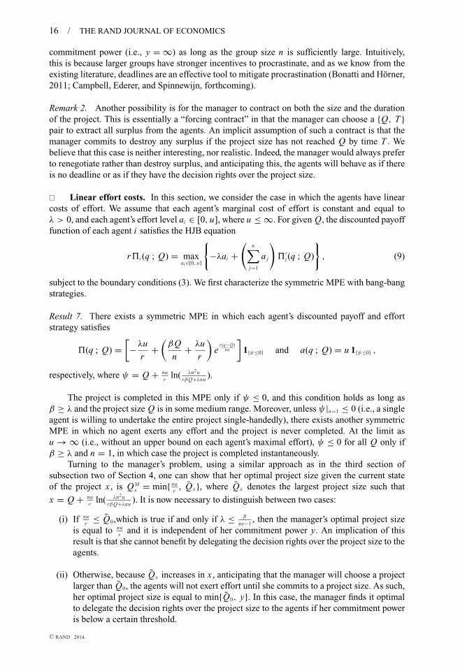
Remark 2. Another possibility is for the manager to contract on both the size and the durationof the project. This is essentially a “forcing contract” in that the manager can choose a {Q, T }pair to extract all surplus from the agents. An implicit assumption of such a contract is that themanager commits to destroy any surplus if the project size has not reached Q by time T . Webelieve that this case is neither interesting, nor realistic. Indeed, the manager would always preferto renegotiate rather than destroy surplus, and anticipating this, the agents will behave as if thereis no deadline or as if they have the decision rights over the project size.
� Linear effort costs. In this section, we consider the case in which the agents have linearcosts of effort. We assume that each agent’s marginal cost of effort is constant and equal toλ > 0, and each agent’s effort level ai ∈ [0, u], where u ≤ ∞. For given Q, the discounted payofffunction of each agent i satisfies the HJB equation
r�i (q ; Q) = maxai ∈[0, u]
{−λai +
(n∑
j=1
a j
)�′
i (q ; Q)
}, (9)
subject to the boundary conditions (3). We first characterize the symmetric MPE with bang-bangstrategies.
Result 7. There exists a symmetric MPE in which each agent’s discounted payoff and effortstrategy satisfies
�(q ; Q) =[−λu
r+(βQ
n+ λu
r
)e
r (q−Q)nu
]1{ψ≤0} and a(q ; Q) = u 1{ψ≤0} ,
respectively, where ψ = Q + nur
ln( λn2urβQ+λnu
).
The project is completed in this MPE only if ψ ≤ 0, and this condition holds as long asβ ≥ λ and the project size Q is in some medium range. Moreover, unless ψ |n=1 ≤ 0 (i.e., a singleagent is willing to undertake the entire project single-handedly), there exists another symmetricMPE in which no agent exerts any effort and the project is never completed. At the limit asu → ∞ (i.e., without an upper bound on each agent’s maximal effort), ψ ≤ 0 for all Q only ifβ ≥ λ and n = 1, in which case the project is completed instantaneously.
Turning to the manager’s problem, using a similar approach as in the third section ofsubsection two of Section 4, one can show that her optimal project size given the current stateof the project x , is QM
x = min{ nur, Qx}, where Qx denotes the largest project size such that
x = Q + nur
ln( λn2urβQ+λnu
). It is now necessary to distinguish between two cases:
(i) If nur
≤ Q0,which is true if and only if λ ≤ β
ne−1, then the manager’s optimal project size
is equal to nur
and it is independent of her commitment power y. An implication of thisresult is that she cannot benefit by delegating the decision rights over the project size to theagents.
(ii) Otherwise, because Qx increases in x , anticipating that the manager will choose a projectlarger than Q0, the agents will not exert effort until she commits to a project size. As such,her optimal project size is equal to min{Q0, y}. In this case, the manager finds it optimalto delegate the decision rights over the project size to the agents if her commitment poweris below a certain threshold.
C© RAND 2014.

GEORGIADIS, LIPPMAN, AND TANG / 17
A natural question is whether this game has other MPE. We answer this question affirmativelyby characterizing, first, an asymmetric MPE with bang-bang strategies, and second, a symmetricMPE in which the agents are indifferent across any effort level along the equilibrium path.
Example 1. Let r = 0.1, u = 10, β = 0.5, Q = 10, n = 4, and λ = 0.1. This game has anasymmetric MPE in which only one agent exerts the maximal effort u at every moment, whereasthe other agents never exert any effort.
More generally, one can construct MPE with bang-bang strategies in which initially, onlyfew agents exert effort, and others join in as the project progresses. This is in contrast to theuniqueness result established in Proposition 1, indicating that the convexity of the effort costsplays a key role in the uniqueness of a (project-completing) MPE.
In addition to equilibria with bang-bang strategies, if the group comprises n ≥ 2 agents,then one can construct equilibria with interior strategies as shown in the following result.
Result 8. Suppose that β
n> λ, n ≥ 2, and u is sufficiently large. Then for any Q, there exists a
symmetric project-completing MPE in which each agent’s discounted payoff and effort strategysatisfies
�(q ; Q) =(β
n− λ
)Q + λq and a(q ; Q) = r
[(β
n− λ
)Q + λq
](n − 1)λ
,
respectively. In contrast, if β
n≤ λ or n = 1, then there exists no symmetric project-completing
MPE with interior strategies.15
This MPE has a flavor of a mixed strategy equilibrium; observe that �′(q ; Q) = λ for allq, so that at every moment, the agents are indifferent across any effort level. Observe that eachagent’s ex ante discounted payoff increases in the project size, which implies that the agents’(and it turns out also the manager’s) optimal project size is equal to ∞. This is intuitive as β
n> λ
implies that each agent’s marginal benefit from a unit of progress exceeds its marginal cost, andthe agents are risk neutral. Finally, it is useful to note that one can construct MPE in which someof the agents use bang-bang strategies, with the others using interior strategies, akin to thosecharacterized in Results 7 and 8, respectively.
6. Concluding remarks
� We propose a tractable model to study the interaction between a group of agents whocollaborate over time to complete a project and a manager who chooses its size. A central featureof the model is that the manager has limited commitment power, in that she can only commit tothe project size when the project is sufficiently close to completion. This is common in projectsthat involve a significant innovation or quality or design component that is difficult to contract onin advance.
In a setting in which both the manager and the agents are rational and they do not obtainnew information about the difficulty or the value of the project, we show that the manager hasincentives to extend the project as it progresses. As a result, if the manager has lower commitmentpower, then she will eventually commit to a bigger project. To mitigate her commitment problem,the manager might consider delegating the decision rights over the project size to the agents,who will choose a smaller project than is optimal for the manager, but their preferences are time-consistent. We show that delegation is optimal unless the manager has sufficient commitmentpower.
15 If u < a(Q ; Q) = r β Qn(n−1)λ
then there exists a symmetric MPE in which the agents’ effort levels are interior up tosome threshold �, while they are equal to u thereafter.
C© RAND 2014.

18 / THE RAND JOURNAL OF ECONOMICS
In our model, agents are compensated upon completion of the project and their compensationis independent of the completion time of the project. Although Georgiadis (2013) shows thatbackloading all rewards is optimal when the project size is given exogenously, it is unclearthat this continues to be the case when the project size is endogenous and the manager haslimited commitment power. It would be interesting to explore whether a more elaborate schemein which the manager provides agents with flow payments while the project is in progress(e.g., Sannikov, 2008) or uses time-dependent contracts (e.g., milestones with deadlines) canimprove her discounted profit. Second, Schelling (1960) made an important observation thatfree-riding is both a commitment problem and an information problem, and although significantadvances have been made to analyze the former, little is known about the latter. Therefore,incorporating asymmetric or incomplete information to this class of games may provide valuableinsights.
Appendix A
In this Appendix, we consider six extensions to our model to test the robustness of the main results.
� Production synergies and team coordination costs. First, we consider the case in which at every moment, thetotal effort of the team is greater (due to production synergies) or smaller (due to coordination costs among the teammembers) than the sum of the agents’ individual efforts. We show that all three main results continue to hold for anydegree of complementarity.
To obtain tractable results, we consider the production function proposed by Bonatti and Horner (2011), so that theproject evolves according to dq = (
∑ni=1 a1/γ
i )γ dt , where γ > 0. Note that γ ∈ (0, 1) (γ > 1) captures the case in whichthe total effort of the team is smaller (greater) than the sum of the agents’ individual efforts, and a larger γ indicatessmaller coordination costs or a stronger degree of complementarity. By assuming symmetric strategies, it follows thatgiven the current state of the project q, cooperation level k, and the completion state Q, each agent’s discounted payoffand effort strategy are given by
�(q ; Q, k) = rn2−2γ
2k
([q − C(Q, k)]+)2
2n − kand a(q ; Q, k) = rn1−γ
2n − k[q − C(Q, k)]+ ,
respectively, where C(Q, k) = Q −√
2βQr
n2γ−2(2n−k)kn
.16 Because (with other things equal) �(q ; Q, k) increases in k forall γ , it follows that for all k ∈ [1, n], there exists a PPE such that each agent follows the strategy dictated by a(q ; Q, k),and after any deviation from the equilibrium path, all agents revert to the MPE; that is, k = 1. Furthermore, each agent’sdiscounted payoff, his equilibrium effort, as well as the aggregate effort of the entire team, increase in the degree ofcomplementarity γ .
By using the agents’ strategies, it follows that the manager’s discounted profit satisfies
W (q ; Q, Q, k) = (1 − β)Q
([q − C(Q, k)]+
Q − C(Q, k)
) 2n−kn
.
To streamline the exposition, we focus on the extreme cases in which the manager has either full or no commitmentpower. It follows that
QMFC = β
r
k(2n − k)
2n
(4n
4n − k
)2
n2γ−2 and QMNC = 2β
r
kn
2n − kn2γ−2 .
Observe that the manager’s optimal project size increases in the degree of complementarity, and similar to the caseanalyzed in Section 4QM
NC > QMFC . Moreover, the counterpart of Proposition 3 continues to hold; that is, if the manager
has less commitment power, then she will choose a bigger project.We now examine the manager’s option to delegate the choice of Q to the agents. To begin, note that the agents’
optimal project size satisfies Q A = β
2rk(2n−k)
nn2γ−2. By following a similar approach as in the third subsection of Section 4,
it follows that there exists a threshold� such that the manager is better off delegating the choice of the project size to theagents if and only if her commitment power y < �.
� Fixed compensation. In the base model, we have assumed that the agents’ net payoff upon completion of theproject is proportional to its value. Whereas a more valuable project will typically yield a larger net payoff to the agents–for
16 As the algebra is straightforward and similar to that used to derive Propositions 1 and 2, it is omitted here in orderto streamline the exposition.
C© RAND 2014.

GEORGIADIS, LIPPMAN, AND TANG / 19
example, a bigger bonus, a salary increase, greater job security, or a larger outside option, this assumption can be thoughtof as an extreme case, as any incentive scheme will likely consist of a fixed component that is independent of the projectsize, and a performance-based component. In this section, we consider the opposite extreme where each agent’s net payoffis fixed and independent of the project size, while efforts are perfect substitutes; that is, dqt = (∑n
i=1 ai,t
)dt .
The main results continue to hold. In fact, the manager’s commitment problem becomes so aggravated in this case,that the project may never be completed in equilibrium. Moreover, because the agents’ net reward is independent of Q,their optimal project size is always 0. As such, the manager can no longer use delegation to mitigate her commitmentproblem.
To begin, suppose that each agent receives a lump sum Vn
as soon as the project is completed regardless of its size.Then given the current state of the project q, the cooperation level k, and the completion state Q, each agent’s equilibriumeffort is given by
a (q ; Q, k) = r
2n − k
[q − C(Q, k)
]+where C(Q, k) = Q −
√2V
r
(2n − k)k
n,
whereas the manager’s discounted profit satisfies
W(q ; Q, Q, k
) = (Q − V )
([q − C(Q, k)]+
Q − C(Q, k
)) 2n−k
n
.
Using the same approach as in Section 3, one can show that for all k ∈ (1, n], there exists a PPE such that each agentfollows the strategy dictated by a (q ; Q, k) contingent on all other agents following the same strategy, and reverts to theMPE (i.e., k = 1) after observing a deviation.
By examining the manager’s optimal project size, it follows that with full and with no commitment power, we have
QMFC = 2n − k
3n − kV + n
3n − k
√2V
r
(2n − k)k
nand QM
NC = V +√
2V
r
kn
2n − k,
respectively. Observe that QMNC > QM
FC , and by solving for QMx ∈ arg maxQ W (q ; Q, Q, k), it follows that QM
x increasesin x . Therefore, similar to the base model, the manager has incentives to extend the project as it progresses. In fact, theseincentives can be so strong that there exists an equilibrium in which the project is not completed. To see why, note thatthe project is completed only if C (Q ; k) < 0, and this inequality is true at Q = QM
NC (k) if and only if r V <2k(n−k)2
n(2n−k).17
Moreover, if each agent’s net payoff is independent of the project size, then delegating the choice of the project size tothe agents is not beneficial, because they will choose a project of size 0.
� Flow payments while the project is in progress. Throughout the analysis, we have maintained the assumption thatthe agents receive a lump-sum payment upon completion of the project, but they do not receive any flow payments whilethe project is in progress. Therefore, to extend the project, the manager must only incur the cost associated with having towait longer until the project is completed. In this section, we consider the case in which the manager compensates eachagent with a flow payment w
n> 0 per unit of time while the project is in progress, in addition to a lump-sum payment
upon completing it, where w is not too large.For a given project size Q, each agent’s discounted payoff, and the manager’s discounted profit satisfy
r�(q ; Q) = w
n+ k(2n − k)
2
[�′(q ; Q)
]2s.t. � (Q ; Q) = βQ
r W(q ; Q, Q
) = −w + [na(q ; Q, k
)]W ′ (q ; Q, Q
)s.t. W
(Q ; Q, Q
) = (1 − β)Q ,
respectively, where a(q ; Q, k) = k�′(q ; Q). As this model is analytically not tractable, to examine how the main resultsextend to this case, we present a numeric illustration (see Figure A1). The takeaway from this analysis is that the mainresults continue to hold when the agents receive flow payments while the project is in progress.
� Variable incentive power. A key assumption of the model is that upon completion of the project, its value issplit among the parties according to a fixed fraction: the manager receives 1 − β of its value, whereas each agentreceives β
n. We have argued that this assumption is important to capture the manager’s limited commitment power
(see the last paragraph in the second section of subsection two of Section 4). Nevertheless, one might still wonderwhat is the impact on the overall dynamics of choosing some alternative class of reward functions. In this section, weconsider the case in which β(q) = β0 + β1q, where β0 ∈ (0, 1), and β1 is either positive or negative, but sufficientlysmall.
For a given Q, the equilibrium characterization is identical to that developed in Section 3. Moreover, it is straight-forward to show that similar to the base model, the agents’ optimal project size is independent of when they committo it. However, determining the manager’s optimal project size is not tractable due to the second term in β(q). As
17 In this case, the manager finds it optimal to commit to a project size equal to y at time 0.
C© RAND 2014.

20 / THE RAND JOURNAL OF ECONOMICS
FIGURE A1
AN EXAMPLE IN WHICH THE MANAGER COMPENSATES THE AGENTS PER UNIT OF TIME WHILETHE PROJECT IS IN PROGRESS WHEN β = 0.5, r = 0.1, n = 4, AND w = 0.001
Opt
imal
pro
ject
siz
e
Man
ager
’s d
isco
unte
d pr
ofit
Commitment power Commitment power
W/oW/
Notes: The left panel illustrates that her optimal project size decreases in her commitment power, whereas the agents’optimal project size is independent of their commitment power. The right panel illustrates that delegating the decisionrights over the project size to the agents is beneficial if and only if the manager doesn’t have sufficient commitment power.
such, we examine how the main results of the article extend to this case numerically. Figure A2 illustrates an exam-ple, which indicates that the main results hold if the agents’ share of the payoff is a (linear) function of the projectsize.
� Sequential projects. Insofar, we have assumed that the manager interacts with the agents for the duration of asingle project. However, because in practice, relationships between a manager and work teams are often persistent, it isimportant to verify that the main results of this article are robust to repeated interactions. In this section, we consider thecase in which as soon as a project is completed, the manager and the agents interact for the duration of another projectwith probability α < 1, whereas the relationship is terminated with probability 1 − α and each party receives its outsideoption, which is normalized to 0.18
Indeed, we find that when the manager and the agents engage in sequential projects, all the main results continueto hold. Moreover, we observe that if the relationship is more persistent (i.e., α is larger), then the manager has strongerincentives to delegate the choice of the project size to the agents.
Because the problem is stationary, the manager will choose the same project size every time. Both the agents’and the manager’s problem remain unchanged, except for the boundary conditions, which become � (Q ; Q) = βQ
n+
α� (0 ; Q) and W(Q ; Q, Q
) = (1 − β)Q + αW(0 ; Q, Q
), respectively. The interpretation of these conditions is that
upon completion of each project, each party receives its net payoff from this project, plus the expected continuation valuefrom future projects.
Unfortunately, it is not possible to derive the desired results analytically. As such, we use a numerical example toillustrate how the main results of the article extend to this case. Figure A3 illustrates that the main results continue tohold. In particular, (i) the manager’s optimal project size decreases in her commitment power, whereas the agents’ optimalproject size is independent of their commitment power, and (ii) the manager should delegate the decision rights over Qunless she has sufficient commitment power.
18 Because the value of the project has been assumed to be linear in its size and it generates a payoff only uponcompletion, as α → 1, both the manager and the agents choose an arbitrarily small project, which is completed arbitrarilyquickly. Therefore, we restrict attention to the cases in which α < 1.
C© RAND 2014.
GEORGIADIS, LIPPMAN, AND TANG / 21
FIGURE A2
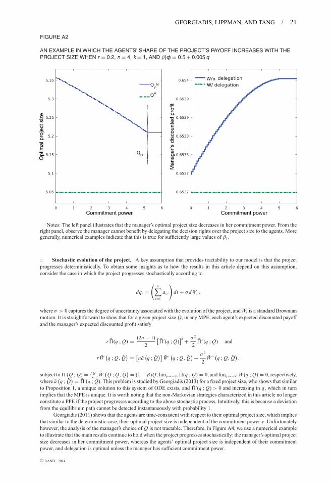
AN EXAMPLE IN WHICH THE AGENTS’ SHARE OF THE PROJECT’S PAYOFF INCREASES WITH THEPROJECT SIZE WHEN r = 0.2, n = 4, k = 1, AND β(q) = 0.5 + 0.005 q
Opt
imal
pro
ject
siz
e
Commitment power Commitment power
Man
ager
’s d
isco
unte
d pr
ofit
W/oW/
Notes: The left panel illustrates that the manager’s optimal project size decreases in her commitment power. From theright panel, observe the manager cannot benefit by delegating the decision rights over the project size to the agents. Moregenerally, numerical examples indicate that this is true for sufficiently large values of β1.
� Stochastic evolution of the project. A key assumption that provides tractability to our model is that the projectprogresses deterministically. To obtain some insights as to how the results in this article depend on this assumption,consider the case in which the project progresses stochastically according to
dqt =(
n∑i=1
ai,t
)dt + σdWt ,
where σ > 0 captures the degree of uncertainty associated with the evolution of the project, and Wt is a standard Brownianmotion. It is straightforward to show that for a given project size Q, in any MPE, each agent’s expected discounted payoffand the manager’s expected discounted profit satisfy
r�(q ; Q) = (2n − 1)
2
[�′(q ; Q)
]2 + σ 2
2�′′(q ; Q) and
r W(q ; Q, Q
) = [na(q ; Q
)]W ′ (q ; Q, Q
)+ σ 2
2W ′′ (q ; Q, Q
),
subject to � (Q ; Q) = βQn
, W(Q ; Q, Q
) = (1 − β)Q, limq→−∞ �(q ; Q) = 0, and limq→−∞ W (q ; Q) = 0, respectively,where a
(q ; Q
) = �′(q ; Q). This problem is studied by Georgiadis (2013) for a fixed project size, who shows that similarto Proposition 1, a unique solution to this system of ODE exists, and �′(q ; Q) > 0 and increasing in q, which in turnimplies that the MPE is unique. It is worth noting that the non-Markovian strategies characterized in this article no longerconstitute a PPE if the project progresses according to the above stochastic process. Intuitively, this is because a deviationfrom the equilibrium path cannot be detected instantaneously with probability 1.
Georgiadis (2011) shows that the agents are time-consistent with respect to their optimal project size, which impliesthat similar to the deterministic case, their optimal project size is independent of the commitment power y. Unfortunatelyhowever, the analysis of the manager’s choice of Q is not tractable. Therefore, in Figure A4, we use a numerical exampleto illustrate that the main results continue to hold when the project progresses stochastically: the manager’s optimal projectsize decreases in her commitment power, whereas the agents’ optimal project size is independent of their commitmentpower, and delegation is optimal unless the manager has sufficient commitment power.
C© RAND 2014.
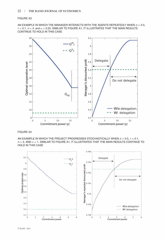
22 / THE RAND JOURNAL OF ECONOMICS
FIGURE A3
AN EXAMPLE IN WHICH THE MANAGER INTERACTS WITH THE AGENTS REPEATEDLY WHEN β = 0.5,r = 0.1, n = 4, and α = 0.25. SIMILAR TO FIGURE A1, IT ILLUSTRATES THAT THE MAIN RESULTSCONTINUE TO HOLD IN THIS CASE
Man
ager
’s d
isco
unte
d pr
ofit
Opt
imal
coo
pera
tion
leve
l
Commitment power (y) Commitment power (y)
W/oW/
FIGURE A4
AN EXAMPLE IN WHICH THE PROJECT PROGRESSES STOCHASTICALLY WHEN β = 0.5, r = 0.1,n = 3, AND σ = 1. SIMILAR TO FIGURE A1, IT ILLUSTRATES THAT THE MAIN RESULTS CONTINUE TOHOLD IN THIS CASE
Opt
imal
pro
ject
siz
e
Man
ager
’s e
xpec
ted
disc
ount
ed p
rofit
Commitment power Commitment power
W/oW/
C© RAND 2014.

GEORGIADIS, LIPPMAN, AND TANG / 23
Appendix B
This Appendix contains all the proofs.
Proof of Proposition 1. To show that a MPE with differentiable strategies exists for this game, it suffices to show thata solution to (4) exists. To show this, we derive a symmetric solution analytically. In particular, for symmetric strategies(i.e., �i (q ; Q) = � j (q ; Q) for all i and j), (4) can be rewritten as
r�(q ; Q) = 2n − 1
2
[�′(q ; Q)
]2, (B1)
and the solution to this ODE satisfies
�(q ; Q) = r
2
([q − C(Q)]+)2
2n − 1, where C(Q) = Q −
√2βQ
r
2n − 1
n
is determined by the value matching condition. By using the first-order condition, it follows that each agent’s effortstrategy is given by
a(q ; Q) = r
2n − 1[q − C(Q)]1{q≥C(Q)} .
To show that there do not exist any asymmetric solutions to (4), we proceed by contradiction. Fix Q > 0, andsuppose there exists at least two agents a and b whose discounted payoff functions �a(q ; Q) and �b(q ; Q) satisfy (4),but�a(q ; Q) �= �b(q ; Q) for at least some q < Q. Then let D(q) = �a(q ; Q) −�b(q ; Q), and note that D(Q) = 0 andD(·) is differentiable. Then using (4), we can write 2r D(q) = [2
∑i �i (q ; Q) −�a(q ; Q) −�b(q ; Q)]D′(q). Moreover,
because agents are impatient (r > 0) and the amount of effort that needs to be exerted until the project is completeddiverges to infinity as q → −∞, it must be true that �i (q ; Q) → 0 as q → −∞. Therefore, limq→−∞ D(q) = 0, so ifD(q) �= 0 for at least some q < Q, then it must be the case that there exists some interior z < Q such that D(z) �= 0 andD′(z) = 0, which yields a contradiction. Hence, we conclude that (4) cannot admit an asymmetric solution.
To show that (B1) has a unique symmetric solution, we use a similar approach. Fix Q > 0, and suppose that thereexists �A(q ; Q) and �B (q ; Q) that both satisfy (B1). Then let �(q) = �A(q ; Q) −�B (q ; Q), and note that �(Q) = 0and �(·) is differentiable. Therefore, (B1) can be rewritten as 2r�(q) = (2n − 1)[�′
A(q ; Q) +�′B (q ; Q)]�′(q). More-
over, limq→−∞ �(q) = 0 by the same argument as above, so if�(q) �= 0 for at least some q < Q, then it must be the casethat there exists some interior z < Q such that �(z) �= 0 and �′(z) = 0, which yields a contradiction. Therefore, thereexists a unique symmetric solution to (4).
We have insofar shown that there exists a unique solution to (4), and that this solution is symmetric. Moreover, notethat if C(Q) ≥ 0 (or equivalently, Q ≥ 2β
r2n−1
n), then the equilibrium strategy dictates that no agent ever exerts any effort,
in which case the project is never completed. On the other hand, as long as C(Q) < 0, the strategy a(q ; Q) constitutesthe unique project-completing MPE. Next, suppose that C(Q) < 0 ≤ C(Q)|n=1 (or equivalently, 2β
r≤ Q < 2β
r2n−1
n), and
fix all effort strategies except that of agent i to 0. Then agent i’s best–response is to also exert 0 effort, as C(Q)|n=1 ≥ 0;that is, he is not willing to undertake the entire project by himself. As a result, if Q ≥ 2β
r, then in addition to the
project-completing MPE, there also exists an equilibrium in which no agent exerts any effort, and the project is nevercompleted.
Finally, to compute the completion time of the project, we substitute the agents’ effort function a(q; Q) intodqt = nat dt , we solve the resulting ODE q ′(t) = r n
2n−1[q(t) − C(Q)]+ subject to q(0) = 0, and we obtain the completion
time of the project τ by solving for q(τ ) = Q. Q.E.D.
Proof of Proposition 2. This proof is organized as follows. First, we show that each agent’s discounted payoff functionis given by �(q ; Q, k) if at every moment, all agents choose their effort level according to (5), and that (6) is thecorresponding effort level. Then we show that there exists a PPE in which each agent’s effort level and discounted payoffsatisfies (6) and �(q ; Q, k) along the equilibrium path, respectively.
From (5), given the current state of the project q, the first-order condition yields a(q ; Q, k) = k�′(q ; Q, k), andthe second-order condition is always satisfied. Substituting the first-order condition into each agent’s HJB equation yields
�(q ; Q k) = (2n − k)k
2r
[�′(q ; Q, k)
]2,
subject to �(Q ; Q, k) ≥ 0 for all q and �(Q ; Q, k) = βQn
.
A solution to the above HJB equation is given by �(q ; Q, k) = r2k
([q−C(Q, k)]+ )2
2n−k, and by using the first-order
condition, it follows that each agent’s effort strategy satisfies (6). If k = 1, then (6) corresponds to the Markov equilibrium.To compute the completion time of the project, we substitute (6) into dqt = nat dt , solving the resulting differentialequation q ′(t) = r n
2n−k[q(t) − C(Q, k)]+ subject to q(0) = 0 yields that q(t) = −C(Q, k)(e
r n t2n−k − 1). By solving for
q(τ ) = Q, we obtain the completion time of the project τ (Q, k) = 2n−krn
ln[1 − QC(Q, k)
].
C© RAND 2014.
24 / THE RAND JOURNAL OF ECONOMICS
We now show that for any k ∈ (1, n], there exists a PPE in which along the equilibrium path, each agent’s effortlevel is given by (6). It follows that in equilibrium, each agent’s discounted payoff satisfies �(q ; Q, k). Because theproject progresses deterministically, there is a one-to-one mapping between t and qt , and it will be convenient to rewrite(6) as a function of time, so that (abusing notation) a(t ; Q, k) = − −rC(Q, k)
2n−ke
r n t2n−k . Fix some Q and k ∈ (1, n], and consider
the following strategy:
at ={
a(t ; Q, k) if qt = −C(Q, k)[e
r n t2n−k − 1
]a(qt ; Q, 1) otherwise,
where a(qt ; Q, k) is given in (6) and qt = ∫ t
0 n a(s ; Q, k)ds. This strategy designates that at every moment t , each agentchooses his effort level by maximizing the discounted payoff of k agents as long as every other agent has insofar followedthis strategy, and he reverts to the MPE otherwise. There is a well-known problem associated with defining such triggerstrategy in continuous-time games. To see why, suppose that a deviation occurs at some t ′, and agents revert to the MPEat some t ′′ > t . Because there is no first moment after t ′, there always exists some t ∈ (t ′, t ′′) such that the agents arebetter off reverting to the MPE at that t ; that is, subgame perfection fails. To resolve this problem, following Bergin andMacLeod (1993), we define the following inertia strategies:
aεt ={
a(t ; Q, k) if qt−ε = −C(Q, k)[e
r n (t−ε)2n−k − 1
]a(qt ; Q, 1) otherwise,
(B2)
where ε > 0 and sufficiently small, and qt = 0 for all t ≤ 0. First, observe that at the limit as ε → 0, aεt converges to at .Second, because aεt < ∞ for all ε, t , Q, and k ∈ (1, n], for any decreasing sequence {εm}∞
m=1 converging to 0, the strategiesaεt form a Cauchy sequence. Third, whereas the strategy in (B2) cannot form a PPE, we shall show that it forms an ε−PPE.To see why, first note that if at every moment all agents choose their effort level according to (5), then given the currentstate of the project q, each agent’s discounted payoff is equal to�(q ; Q, k). Moreover,�(q ; Q, k) > �(q ; Q, 1) for allq ≥ C(Q, k) and k > 1. Second, observe that for sufficiently small ε, the optimal strategy against (B2) is for an agent tochoose a(t ; Q, k) at every t < τ , and deviate to the MPE (so that he maximizes his discounted payoff given the currentstate of the project) at t = τ , where τ is chosen such that the project is completed at τ + ε when the agents follow (B2).In this case, project completion is delayed by at most ε units of time, and each agent’s discounted payoff when the state ofthe project is equal to q is at least �(q ; Q, k) − εr e−rτ (Q, k) − ε
2[a(Q ; Q, k)]2. Therefore, the strategy in (B2) forms an
ε−PPE, and by applying Theorem 3 of Bergin and MacLeod (1993), it follows that the limit strategy as ε → 0 forms aPPE. Consequently, there exists a PPE such that along the equilibrium path, each agent’s effort level is given by (6), andhis discounted payoff satisfies �(q ; Q, k). Q.E.D.
Proof of Proposition 3. To begin, fix k ∈ [1, n], and note that for any x , W (x ; Q, Q, k) is strictly concave in Q. Applyingthe first-order condition yields (8). It is straightforward to verify that ∂
∂xQM
x ∈ (0, 1) and ∂2
∂x2 QMx < 0 for all q > 0. Finally,
solving the fixed point QMQ = Q yields QM
Q = β
r2kn
2n−k.
Next, let g(x) = QMx − x , and observe that g(0) = QM
0 > 0 and g(QMQ ) = 0. Moreover, it is easy to check that
g′(x) < 0 on [0, QMQ ], which implies that given any y ≤ QM
0 , there exists a unique x(y) such that g(x(y)) = y.Clearly, if y ≥ QM
0 , then the manager finds it optimal to commit to QM0 at x = 0. Therefore, for all y ≥ 0, there
exists a unique x(y) that solves max{QMx(y) − y, 0} = x(y). Furthermore, noting that ∂
∂xQM
x ∈ (0, 1), it follows that x(y)and QM
x(y) both decrease in y.To proceed, suppose that y < QM
0 , and note that W (q ; Q, Q) is strictly concave in Q for all Q ≥ q. Given thecurrent state of the project q, the manager can either commit to a completion state in the interval [q, q + y], in which caseher discounted payoff is equal to maxq≤Q≤q+y W (q , Q, Q), or she can delay committing, anticipating that she will be ableto commit to some completion state q ′ > q + y later, which will yield her a discounted payoff W (q , q ′, q ′). Therefore, themanager will choose to commit to a completion state at q if and only if maxq≤Q≤q+y W (q , Q) ≥ W (q , q ′, q ′) for all q ′ >q + y, or equivalently if and only if arg maxQ≥q W (q , Q, Q) ≤ q + y. By noting that QM
q ∈ arg maxQ≥q{W (q ; Q, Q)},it follows that the manager finds it optimal to commit to project size QM
x(y) at q = x(y), where x(y) is the unique solutionto the equation max{QM
x(y) − y, 0} = x(y), and QMx(y) is given by (8). Q.E.D.
Proof of Proposition 4. To begin, fix n ≥ 1 and k ∈ [1, n]. If the project size is chosen by the agents, then they willchoose Q A = β
rk(2n−k)
2n, and by substituting this into the manager’s expected discounted profit, yields W (0 ; Q A, Q A) =
(1−β)βr
k(2n−k)2n
( 12)
2n−kn .
Next, consider the case in which the completion state is chosen by the manager, and she has no commitment power(i.e., y = 0) so that she eventually completes the project at QM
NC = β
r2kn
2n−k. By substituting this, the manager’s expected
discounted profit we have that W (0 ; QMNC, QM
NC) = (1−β)βr
2kn2n−k
( n−k2n−k
)2n−k
n .
Now consider the ratioW (0 ;QM
NC ,QMNC )
W (0 ;Q A ,Q A )= ( 2n
2n−k)2( 2n−2k
2n−k)
2n−kn , and for the purpose of this proof, let h(n, k) =
( 2n2n−k
)2( 2n−2k2n−k
)2n−k
n . Observe that h(k, k) = 0 and limn→∞ h(n, k) = 1. Differentiating with respect to n yields ddn
h(n, k) =4[(2n−k)(n−k) ln( 2n−2k
2n−k )+nk]
(2n−k)3(n−k)( 2n−2k
2n−k)
2n−1n > 0 if and only if (2n − k)(n − k) ln( 2n−2k
2n−k) + nk > 0 or equivalently if ln ( 2n−2k
2n−k) +
nk(2n−k)(n−k)
> 0. Now observe that limn→∞ [ln ( 2n−2k2n−k
) + nk(2n−k)(n−k)
] = 0, and ∂
∂n[ln ( 2n−2k
2n−k) + nk
(2n−k)(n−k)] < 0 for all n ≥ k.
C© RAND 2014.

GEORGIADIS, LIPPMAN, AND TANG / 25
This implies that ln ( 2n−2k2n−k
) + nk(2n−k)(n−k)
> 0, and hence ddn
h(n, k) > 0. By noting that h(k, k) = 0 and limn→∞ h(n, k) = 1,
it follows that h(n, k) < 1 for all n ≥ k, which implies that W (0 ; Q A, Q A) > W (0 ; QMNC, QM
NC) for all n ≥ k.We have thus far established that W (0 ; Q A, Q A) > W (0 ; QM
NC, QMNC). Moreover, it is straightforward to verify that
W (0 ; QMFC, QM
FC) > W (0 ; Q A, Q A); that is, the manager should not delegate the choice of Q to the agents if she has fullcommitment power. Because QM (y) is strictly decreasing in y for all y < QM
FC , W (0 ; Q, Q) is strictly concave in Q, andQM
FC < QMNC , it follows that W (0 ; QM (y), QM (y)) is strictly increasing in y on [0, QM
FC). By noting that W (0 ; Q A, Q A) isindependent of y, it follows that there exists some threshold � < QM
FC such that W (0 ; Q A, Q A) > W (0 ; QM (y), QM (y))if and only if y < �. Q.E.D.
Proof of Proposition 5. Fix some x ∈ [max{Q A, QM (y)|k=1}, QM (y)). By Proposition 2, there exists a PPE in which theagents choose their effort to maximize the discounted payoff of k agents at every t such that qt < x , and they revert to theMPE at qt = x . Now observe that by reverting to the MPE, the agents cannot induce the manager to choose a project sizesmaller than QM (y)|k=1. Moreover, if the state of the project is qt and the agents are playing the MPE, then the manager’sbest–response is to complete the project at Q = max{qt , QM (y)|k=1}. Therefore, there exists a SPE in which the agentsswitch to the MPE at qt = x , and the manager best-responds by completing the project instantaneously. Q.E.D.
Proof of Proposition 6. We use Pontryagin’s maximum principle to characterize a MPE. The Hamiltonian associated witheach agent i’s objective function can be written as
Hi,t = −e−r ta2
i,t
2+ λi,t
(n∑
j=1
a j,t
),
where λi,t ≥ 0 is the costate variable associated with agent i’s Hamiltonian, and his bequest function is φi,T = βQn
e−rT .By Pontryagin’s principle, for each agent i , there exists a continuous function λi,t that satisfies the following conditions forall t ≥ 0: (i) the optimality equation d Hi,t
dai,t= 0; (ii) the adjoint equation λi,t = − d Hi,t
dq; and (iii) the transversality condition
λi,T = dφi,T
d Q. The optimality equation implies that ai,t = λi,t ert , and the adjoint equation can be rewritten as
λi,t = −∑j �=i
d Hi,t
da j,t
da j,t
dt
dt
dq= −
∑j �=i
λi,t
(rλ j,t + λ j,t
)∑n
l=1 λl,t
⇒ λt = −rn − 1
2n − 1λt ,
where the last equality follows from the restriction to symmetric equilibria (and hence, we drop the subscript i). A solutionto the adjoint equation is λt = c e−r t n−1
2n−1 , and by using the transversality condition to determine the constant c, it followsthat c = β
ne
r n T2n−1 . Therefore, each agent’s effort function satisfies the desired expression, and the state of the project at
the deadline is equal to qT = ∫ T
0 nat dt = β
r2n−1
n(1 − e− r n T
2n−1 ). Finally, it is straightforward to verify that the maximizedHamiltonian in concave is q, which implies that this solution does indeed constitute a MPE. Q.E.D.
Proof of Result 6. The manager’s optimal project duration T ∗ follows by taking the first-order condition of W (0 ; T ) withrespect to T , and noting that the second-order condition is satisfied. The project size at t = T ∗ follows by substituting T ∗
into the expression for qT derived in Proposition 6. By substituting T ∗ and qT ∗ into W (0 ; T ), it follows that
W (0 ; T ∗) = (1 − β)β
r
(2n − 1
3n − 1
) 3n−1n
,
and it is straightforward to verify that W (0 ; T ∗) ≥ W (0 ; Q A, Q A) = (1−β)βr
2n−12n
( 12)
2n−1n for all n, with strict inequality
holding for all n ≥ 2. Q.E.D.
Proof of Result 7. Taking the first-order condition in (9) with respect to ai yields that agent i finds it optimal to exerteffort u if �′
i (q ; Q) ≥ λ, whereas he exerts no effort otherwise. By substituting this into (9), assuming symmetry andsolving the resulting ODE yields the desired discounted payoff function. Differentiating this with respect to q yields that�′
i (q ; Q) ≥ λ if and only if q ≥ Q + nur
ln( λn2urβQ+λnu
) = ψ , and by noting that q0 = 0 and �′i (q ; Q) increases in q, it
follows that each agent always exerts the maximal effort u if and only if ψ ≤ 0. Q.E.D.
Proof of Example 1. Suppose that one agent (say, i = 1) exerts the maximal effort u at every moment, whereas the otheragents (i.e., i = 2, . . . , n) never exert any effort. Then it follows from (9) that
�1(q ; Q) = −λu
r+(βQ
n+ λu
r
)e
r(q−Q)u , and
for all i = 2, . . . , n, �i (q ; Q) = βQ
ne
r(q−Q)u .
C© RAND 2014.
26 / THE RAND JOURNAL OF ECONOMICS
Noting that �′i (q ; Q) increases in q, for this set of strategies to constitute a MPE, it must be the case that �′
1(0 ; Q) ≥λ > �′
i (Q ; Q) for all i = 2, . . . , n, or equivalently, that
r
u
(βQ
n+ λu
r
)e− r Q
u ≥ λ >r
u
βQ
n.
It is straightforward to verify that these inequalities are satisfied when r = 0.1, u = 10, β = 0.5, Q = 10, n = 4, andλ = 0.1. Q.E.D.
Proof of Result 8. Let us guess that there exists a symmetric MPE in which for given Q, �′(q ; Q) = λ for all q.Integrating with respect to q and solving for the boundary condition yields that�(q ; Q) = ( β
n− λ)Q + λq. Substituting
this into (9) and solving for each agent’s effort level yields that a(q ; Q) = r [( βn −λ)Q+λq]
(n−1)λ. By noting that the second-order
condition is satisfied, it follows that this strategy does indeed constitute a MPE. Q.E.D.
References
ADMATI, A.R. AND PERRY, M. “Joint Projects without Commitment.” Review of Economic Studies, Vol. 58 (1991), pp.259–276 .
AGHION, P. AND TIROLE, J. “The Management of Innovation.” Quarterly Journal of Economics, Vol. 109 (1994), pp.1185–1209.
———. “Formal and Real Authority in Organizations.” Journal of Political Economy, Vol. 105 (1997), pp. 1–29.AKERLOF, G.A. AND KRANTON, R.E. “Economics and Identity.” Quarterly Journal of Economics, Vol. 115 (2000), pp.
715–753.AL-NAJJAR, N.I., ANDERLINI, L., AND FELLI, L. “Undescribable Events.” Review of Economic Studies, Vol. 73 (2006), pp.
849–868.BERGIN, J. AND MACLEOD, W.B. “Continuous Time Repeated Games.” International Economic Review, Vol. 43 (1993),
pp. 21–37.BONATTI, A. AND HORNER, J. “Collaborating.” American Economic Review, Vol. 101 (2011), pp. 632–663.BRENNER, R. “Are You Changing Tactics or Moving the Goal Posts?” www.chacocanyon.com/pointlookout/011219.shtml,
2001. Accessed November 12, 2013.———. “Private Communication.” Principal, Chaco Canyon Consulting, 2013.CAMPBELL, A., EDERER, F.P., AND SPINNEWIJN, J. “Delay and Deadlines: Freeriding and Information Revelation in Part-
nerships.” American Economic Journal: Microeconomics (forthcoming).DESSEIN, W. “Authority and Communication in Organizations.” Review of Economic Studies, Vol. 69 (2002), pp. 811–838.DIXIT, A. The Art of Smooth Passing. Bedford, UK: Taylor & Francis, 1999.FERSHTMAN, C. AND NITZAN, S. “Dynamic Voluntary Provision of Public Goods.” European Economic Review, Vol. 35
(1991), pp. 1057–1067.FREIXAS, X., GUESNERIE, R., AND TIROLE, J. “Planning under Incomplete Information and the Ratchet Effect.” Review of
Economic Studies, Vol. 52 (1985), pp. 173–191.HART, O. AND MOORE, J. “Property Rights and the Nature of the Firm.” Journal of Political Economy, Vol. 98 (1990), pp.
1119–1158.GEORGIADIS, G. “Projects and Team Dynamics.” Unpublished manuscript, 2011.———. “Projects and Team Dynamics.” Working Paper, 2013.GROSSMAN, S.J. AND HART, O.D. “The Cost and Benefits of Ownership: A Theory of Vertical and Lateral Integration.”
Journal of Political Economy, Vol. 94 (1986), pp. 691–719KESSING, S.G. “Strategic Complementarity in the Dynamic Private Provision of a Discrete Public Good.” Journal of
Public Economic Theory, Vol. 9 (2007), pp. 699–710.LAFFONT, J-J. AND TIROLE, J. “The Dynamics of Incentive Contracts.” Econometrica, Vol. 56 (1988), pp. 1153–1175.MARX, L.M. AND MATTHEWS, S.A. “Dynamic Voluntary Contribution to a Public Project.” Review of Economic Studies,
Vol. 67 (2000), pp. 327–358.SANNIKOV, Y., “A Continuous-Time Version of the Principal-Agent Problem.” Review of Economic Studies, Vol. 75 (2008),
pp. 957–984.SCHELLING, T.C. The Strategy of Conflict. Cambridge, MA: Harvard University Press, 1960.TAJFEL, H. AND TURNER, J.C. “An Integrative Theory of Intergroup Conflict.” In W.G. Austin and S. Worchel, eds., The
Social Psychology of Intergroup Relations. Monterey, CA: Brooks/Cole Publishing, 1979.TANG, C.S. AND ZIMMERMAN, J. “Managing New Product Development and Supply Chain Risks: The Boeing 787
Case.”Supply Chain Forum: An International Journal, Vol. 10 (2009), pp. 74–86.TIROLE, J. “Incomplete Contracts: Where Do We Stand?” Econometrica, Vol. 67 (1999), pp. 741–781.Wired Magazine. “The Birth of the iPod.” http://archive.wired.com/gadgets/mac/news/2004/07/64286, 2004. Accessed
December 8,k 2013,YILDIRIM, H. “Getting the Ball Rolling: Voluntary Contributions to a Large Scale Public Project.” Journal of Public
Economic Theory, Vol. 8 (2006), pp. 503–528.
C© RAND 2014.