Project scheduling with irregular costs: complexity, approximability, and algorithms

Digital Object Identifier (DOI) 10.1007/s00236-004-0150-2Acta Informatica 41, 83–97 (2004)

Project scheduling with irregular costs:complexity, approximability, and algorithms

Alexander Grigoriev1, Gerhard J. Woeginger2

1 Department of Quantitative Economies, University of Maastricht, P.O. Box 616,6200 MD Maastricht, The Netherlands(e-mail: [email protected])

2 Department of Mathematics and Computer Science, Eindhoven University of Technology,P.O. Box 513, 5600 MB Eindhoven, The Netherlands(e-mail: [email protected])

Received: 2 February 2004 / 13 September 2004Published online: 29 October 2004 – c© Springer-Verlag 2004

Abstract. We address a generalization of the classical discrete time-costtradeoff problem where the costs are irregular and depend on the startingand the completion times of the activities. We present a complete picture ofthe computational complexity and the approximability of this problem forseveral natural classes of precedence constraints. We prove that the problemis NP-hard and hard to approximate, even in case the precedence constraintsform an interval order. For precedence constraints with bounded height,there is a complexity jump from height one to height two: For height one,the problem is polynomially solvable, whereas for height two, it is NP-hardand APX-hard. Finally, the problem is shown to be polynomially solvableif the precedence constraints have bounded width or are series parallel.

1 Introduction

Due to its practical importance, the discrete time-cost tradeoff problem forproject networks has been studied in various contexts by many researchersover the last fifty years; see Kelley & Walker (1959) for an early reference.The modern treatment of this problem started with the dynamic program-ming approaches of Hindelang & Muth (1979) and Robinson (1975), andwith an enumeration algorithm by Harvey & Patterson (1979). An up-to-date overview on the discrete time-cost tradeoff problem is Chapter 4 of thesurvey by Brucker, Drexl, Mohring, Neumann & Pesch (1999) or Chapter 8of the book by Demeulemeester & Herroelen (2002). In this paper, we look

84 A. Grigoriev, G.J. Woeginger

at a generalization of the classical discrete time-cost tradeoff problem wherethe costs depend on the exact starting and completion times of the activities.

Statement of the problem. Formally, we consider instances that are calledprojects and that consist of a finite set A = {A1, . . . , An} of activities to-gether with a partial order ≺ on A. All activities are available for processingat time zero, and they must be completed before a global project deadline T .Hence, the set of possible starting and completion times of the activities is{0, 1, . . . , T}. The set of intervals over {0, 1, . . . , T} (the so-called realiza-tions of the activities) is denoted by R = {(x, y) | 0 ≤ x ≤ y ≤ T}. For ev-ery activity Aj , there is a corresponding cost function cj : R → R

+∪{±∞}that specifies for every realization (x, y) ∈ R a non-negative cost cj(x, y)that is incurred when the activity is started at time x and completed at timey. A realization of the project is an assignment of the activities in A to theintervals in R.A realization is feasible if it obeys the precedence constraints:For any Ai and Aj with Ai ≺ Aj , activity Aj is not started before activityAi has been completed. The cost of a realization is the sum of the costsof all activities in this realization. The goal is to find a feasible realizationof minimum cost. This problem is called min-cost project scheduling withirregular costs, or min-cost PSIC for short.

A closely related problem is max-profit project scheduling with irregularcosts, or max-profit PSIC for short. Instead of cost functions cj for activityAj , here we have profit functions pj : R → R

+ ∪ {±∞} that specify forevery realization of Aj the resulting profit. The goal is to find a feasiblerealization of maximum profit. Such a profit may for instance representthe cost reduction for the project, if a deadline is stretched and an activitybecomes less urgent. Clearly, the min-cost and the max-profit version arepolynomial time equivalent: The transformations cj := const1 − pj andpj := const2−cj with sufficiently large constants const1 and const2 translateone version into the other. However, the two versions seem to behave quitedifferently with respect to their approximability.

Special cases and related problems. Various special cases arise if the costand profit functions satisfy additional properties. A cost function c is mono-tone, if [x1, y1] ⊆ [x2, y2] implies c(x1, y1) ≥ c(x2, y2). A profit functionp is monotone, if [x1, y1] ⊆ [x2, y2] implies p(x1, y1) ≤ p(x2, y2). Theintuition behind these concepts is that short and quick executions should bemore expensive than long and slow executions. It is readily seen that thegeneral version of PSIC is equivalent to the monotone version with respectto computational complexity and approximability.

Another interesting special case arises, if y1 − x1 = y2 − x2 impliesc(x1, y1) = c(x2, y2) and p(x1, y1) = p(x2, y2). In this special case, thecost and the profit of an activity only depend on the length of its realization.

Project scheduling with irregular costs 85

This special case actually is equivalent to the DEADLINE problem for thediscrete time-cost tradeoff problem: The deadline T is hard, and the goal isto assign lengths to activities such that the overall cost is minimized. Onlyrecently, De, Dunne, Gosh & Wells (1997) proved that this problem is NP-hard in the strong sense. Skutella (1998) gives some positive approximabilityresults, and Deineko & Woeginger (2001) give some inapproximability re-sults for bicriteria versions. All negative results in this paper are proved forthe DEADLINE problem, the weakest variant of PSIC. All positive resultsin this paper are proved for the most general version of PSIC.

In another special case, for every activity Aj there is a number Lj suchthat cj(x, y) < ∞ if and only if y−x = Lj . In other words, activity Aj mustbe realized by an interval of length exactly Lj . This special case is classicalproject scheduling with fixed processing times. Chang & Edmonds (1985)proved that this case is polynomial time equivalent to the min-cut problemin graphs; hence, this case is polynomially solvable. Project schedulingwith fixed processing times and some of its variants were also studied byManiezzo & Mingozzi (1999) and by Mohring, Schulz, Stork & Uetz (2001).

Our results. We derive several positive and negative statements on the com-plexity and the approximability of min-cost and max-profit PSIC for severalnatural classes of precedence constraints. Our results are the following:

(1) Interval orders (Section 2). The min-cost and the max-profit version of theDEADLINE problem (and of their PSIC generalizations) are NP-hard andinapproximable even for interval orders.We establish a close (approximationpreserving) connection of the min-cost DEADLINE problem to minimumvertex cover and of the max-profit DEADLINE problem to maximum in-dependent set. All inapproximability results for these graph problems carryover to the DEADLINE problems. As an immediate consequence, unlessP=NP the min-cost DEADLINE problem can not have a polynomial timeapproximation algorithm with worst case ratio strictly better than 7/6. Thisis quite an improvement over an earlier inapproximability result of Deineko& Woeginger (2001) that only established APX-hardness for this problem.

(2) Orders of bounded height (Section 3). If the height of the precedenceconstraints is bounded by 2, then the DEADLINE problems and its PSICgeneralizations are NP-hard and inapproximable. However, if the height ofthe precedence constraints is bounded by 1, then min-cost and max-profitPSIC both can be solved in polynomial time. The main idea is to translatethese project scheduling problems into a maximum weight independent setproblem in an underlying vertex-weighted bipartite graph.

(3) Orders of bounded width (Section 4). If the width of the precedence con-straints is bounded by some fixed constant d, then min-cost and max-profit


PSIC both can be solved in polynomial time O(ndT 2d+1). The algorithm isbased on simple dynamic programming over the time axis, but the detailsare somewhat messy.

(4) Series parallel orders (Section 5). For series parallel precedence con-straints, min-cost and max-profit PSIC can be solved in polynomial timeO(nT 3) by dynamic programming. This result builds on the approaches ofFrank, Frisch, van Slyke & Chou (1970) and Rothfarb, Frank, Rosenbaum,Steiglitz & Kleitman (1970) for the classical discrete time-cost tradeoffproblem, and extends them to the more general problems max-profit andmin-cost PSIC.

(5) Finally in Section 6, we discuss how the complexity of min-cost and max-profit PSIC depends on the encoding of the input. We present an example ofPSIC with two activities A and B, with the precedence constraint A ≺ B,and with (very) specially defined cost/profit functions. For this example,even the DEADLINE problem is NP-hard.

Technical remarks. For costs and profits we allow any values from R+ ∪

{±∞}, that is the non-negative numbers together with plus/minus infin-ity. This should be seen as a useful and simple convention for specifyingthe input: Whenever a cost equals +∞ or a profit equals −∞, then thecorresponding realization is forbidden. Of course this convention leads toinstances that do not have any feasible realization with finite cost or profit,but these instances are easily recognized and singled out in polynomial timeby the following greedy algorithm: “In every step, select a yet unrealizedactivity A for which all predecessors have already been realized. Choose forA the realization (x, y) of finite cost (respectively, finite profit) with small-est value y.” This algorithm gets stuck if and only if there is no projectrealization of finite cost (respectively, finite profit).

Hence, throughout the paper we will restrict ourselves to instances thatallow at least one realization in which all costs (respectively, all profits)are non-negative reals. A more compact representation of the input onlyspecifies those realizations of activities that have finite costs/profits.

2 Interval orders

In this section we will derive a number of negative results for problemPSIC under interval orders. An interval order on a set A = {A1, . . . , An} isspecified by a set of n intervals I1, . . . , In along the real line. Then Ai → Aj

holds if and only if the interval Ii lies completely to the left of the intervalIj , or if the right endpoint of Ii coincides with the left endpoint of Ij . Seee.g. Mohring (1989).


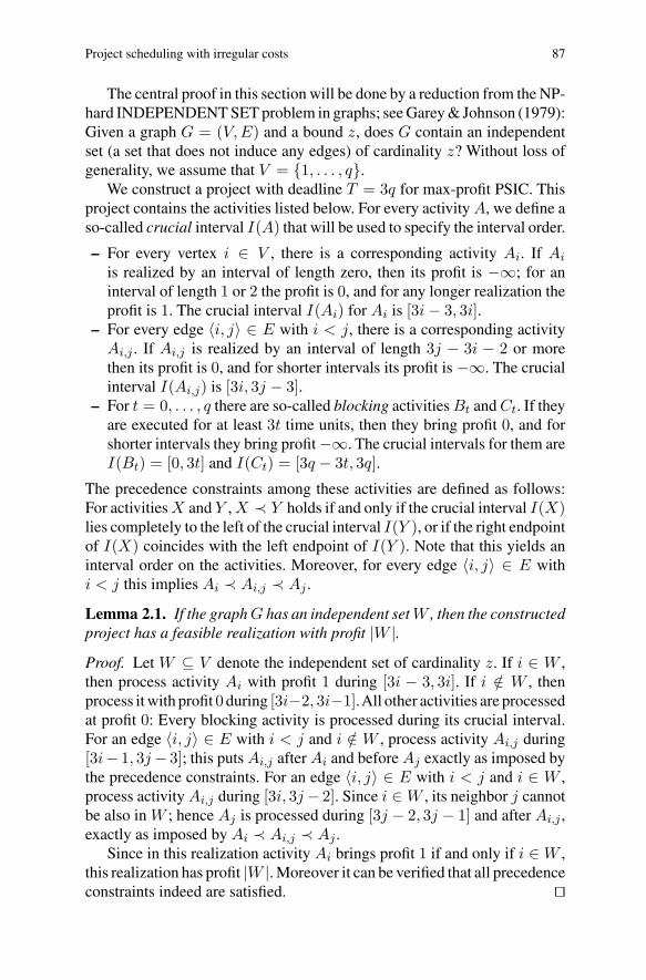
The central proof in this section will be done by a reduction from the NP-hard INDEPENDENT SET problem in graphs; see Garey & Johnson (1979):Given a graph G = (V, E) and a bound z, does G contain an independentset (a set that does not induce any edges) of cardinality z? Without loss ofgenerality, we assume that V = {1, . . . , q}.

We construct a project with deadline T = 3q for max-profit PSIC. Thisproject contains the activities listed below. For every activity A, we define aso-called crucial interval I(A) that will be used to specify the interval order.

– For every vertex i ∈ V , there is a corresponding activity Ai. If Ai

is realized by an interval of length zero, then its profit is −∞; for aninterval of length 1 or 2 the profit is 0, and for any longer realization theprofit is 1. The crucial interval I(Ai) for Ai is [3i − 3, 3i].

– For every edge 〈i, j〉 ∈ E with i < j, there is a corresponding activityAi,j . If Ai,j is realized by an interval of length 3j − 3i − 2 or morethen its profit is 0, and for shorter intervals its profit is −∞. The crucialinterval I(Ai,j) is [3i, 3j − 3].

– For t = 0, . . . , q there are so-called blocking activities Bt and Ct. If theyare executed for at least 3t time units, then they bring profit 0, and forshorter intervals they bring profit −∞. The crucial intervals for them areI(Bt) = [0, 3t] and I(Ct) = [3q − 3t, 3q].

The precedence constraints among these activities are defined as follows:For activities X and Y , X ≺ Y holds if and only if the crucial interval I(X)lies completely to the left of the crucial interval I(Y ), or if the right endpointof I(X) coincides with the left endpoint of I(Y ). Note that this yields aninterval order on the activities. Moreover, for every edge 〈i, j〉 ∈ E withi < j this implies Ai ≺ Ai,j ≺ Aj .

Lemma 2.1. If the graph G has an independent set W , then the constructedproject has a feasible realization with profit |W |.Proof. Let W ⊆ V denote the independent set of cardinality z. If i ∈ W ,then process activity Ai with profit 1 during [3i − 3, 3i]. If i /∈ W , thenprocess it with profit 0 during [3i−2, 3i−1].All other activities are processedat profit 0: Every blocking activity is processed during its crucial interval.For an edge 〈i, j〉 ∈ E with i < j and i /∈ W , process activity Ai,j during[3i− 1, 3j − 3]; this puts Ai,j after Ai and before Aj exactly as imposed bythe precedence constraints. For an edge 〈i, j〉 ∈ E with i < j and i ∈ W ,process activity Ai,j during [3i, 3j − 2]. Since i ∈ W , its neighbor j cannotbe also in W ; hence Aj is processed during [3j − 2, 3j − 1] and after Ai,j ,exactly as imposed by Ai ≺ Ai,j ≺ Aj .

Since in this realization activity Ai brings profit 1 if and only if i ∈ W ,this realization has profit |W |. Moreover it can be verified that all precedenceconstraints indeed are satisfied. ��


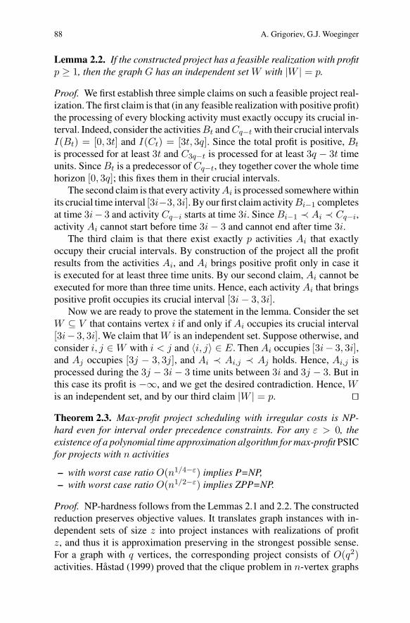
Lemma 2.2. If the constructed project has a feasible realization with profitp ≥ 1, then the graph G has an independent set W with |W | = p.

Proof. We first establish three simple claims on such a feasible project real-ization. The first claim is that (in any feasible realization with positive profit)the processing of every blocking activity must exactly occupy its crucial in-terval. Indeed, consider the activities Bt and Cq−t with their crucial intervalsI(Bt) = [0, 3t] and I(Ct) = [3t, 3q]. Since the total profit is positive, Bt

is processed for at least 3t and C3q−t is processed for at least 3q − 3t timeunits. Since Bt is a predecessor of Cq−t, they together cover the whole timehorizon [0, 3q]; this fixes them in their crucial intervals.

The second claim is that every activity Ai is processed somewhere withinits crucial time interval [3i−3, 3i]. By our first claim activity Bi−1 completesat time 3i − 3 and activity Cq−i starts at time 3i. Since Bi−1 ≺ Ai ≺ Cq−i,activity Ai cannot start before time 3i − 3 and cannot end after time 3i.

The third claim is that there exist exactly p activities Ai that exactlyoccupy their crucial intervals. By construction of the project all the profitresults from the activities Ai, and Ai brings positive profit only in case itis executed for at least three time units. By our second claim, Ai cannot beexecuted for more than three time units. Hence, each activity Ai that bringspositive profit occupies its crucial interval [3i − 3, 3i].

Now we are ready to prove the statement in the lemma. Consider the setW ⊆ V that contains vertex i if and only if Ai occupies its crucial interval[3i− 3, 3i]. We claim that W is an independent set. Suppose otherwise, andconsider i, j ∈ W with i < j and 〈i, j〉 ∈ E. Then Ai occupies [3i − 3, 3i],and Aj occupies [3j − 3, 3j], and Ai ≺ Ai,j ≺ Aj holds. Hence, Ai,j isprocessed during the 3j − 3i − 3 time units between 3i and 3j − 3. But inthis case its profit is −∞, and we get the desired contradiction. Hence, Wis an independent set, and by our third claim |W | = p. ��Theorem 2.3. Max-profit project scheduling with irregular costs is NP-hard even for interval order precedence constraints. For any ε > 0, theexistence of a polynomial time approximation algorithm for max-profit PSICfor projects with n activities

– with worst case ratio O(n1/4−ε) implies P=NP,– with worst case ratio O(n1/2−ε) implies ZPP=NP.

Proof. NP-hardness follows from the Lemmas 2.1 and 2.2. The constructedreduction preserves objective values. It translates graph instances with in-dependent sets of size z into project instances with realizations of profitz, and thus it is approximation preserving in the strongest possible sense.For a graph with q vertices, the corresponding project consists of O(q2)activities. Hastad (1999) proved that the clique problem in n-vertex graphs


(and hence also the independent set problem in the complement of n-vertexgraphs) cannot have a polynomial time approximation algorithm with worstcase guarantee O(n1/2−ε) unless P=NP, and it cannot have a polynomialtime approximation algorithm with worst case guarantee O(n1−ε) unlessZPP=NP. Since the blow-up in our construction is only quadratic, the theo-rem follows. ��

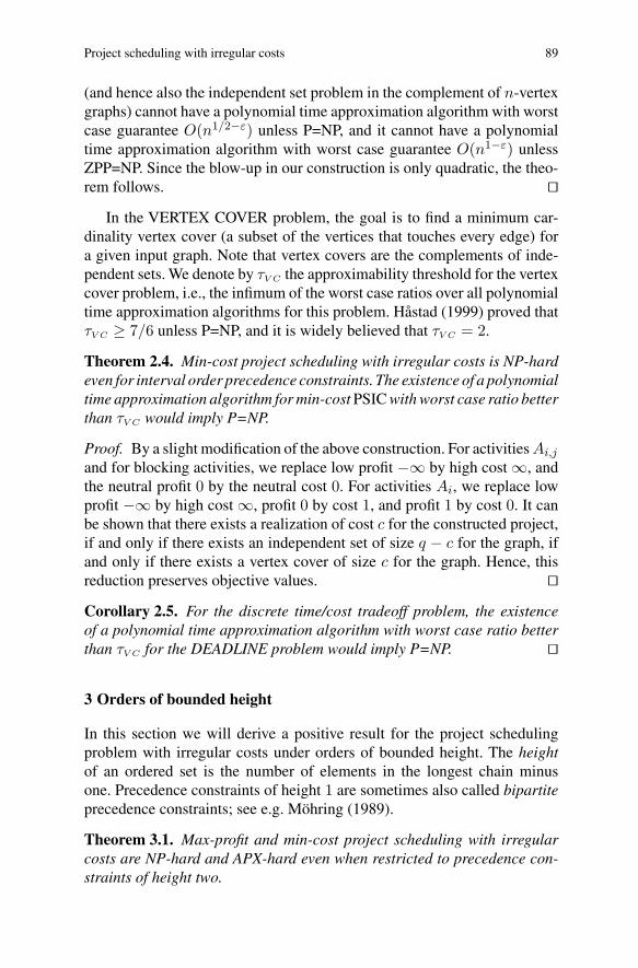
In the VERTEX COVER problem, the goal is to find a minimum car-dinality vertex cover (a subset of the vertices that touches every edge) fora given input graph. Note that vertex covers are the complements of inde-pendent sets. We denote by τV C the approximability threshold for the vertexcover problem, i.e., the infimum of the worst case ratios over all polynomialtime approximation algorithms for this problem. Hastad (1999) proved thatτV C ≥ 7/6 unless P=NP, and it is widely believed that τV C = 2.

Theorem 2.4. Min-cost project scheduling with irregular costs is NP-hardeven for interval order precedence constraints. The existence of a polynomialtime approximation algorithm for min-cost PSIC with worst case ratio betterthan τV C would imply P=NP.

Proof. By a slight modification of the above construction. For activities Ai,j

and for blocking activities, we replace low profit −∞ by high cost ∞, andthe neutral profit 0 by the neutral cost 0. For activities Ai, we replace lowprofit −∞ by high cost ∞, profit 0 by cost 1, and profit 1 by cost 0. It canbe shown that there exists a realization of cost c for the constructed project,if and only if there exists an independent set of size q − c for the graph, ifand only if there exists a vertex cover of size c for the graph. Hence, thisreduction preserves objective values. ��Corollary 2.5. For the discrete time/cost tradeoff problem, the existenceof a polynomial time approximation algorithm with worst case ratio betterthan τV C for the DEADLINE problem would imply P=NP. ��

3 Orders of bounded height

In this section we will derive a positive result for the project schedulingproblem with irregular costs under orders of bounded height. The heightof an ordered set is the number of elements in the longest chain minusone. Precedence constraints of height 1 are sometimes also called bipartiteprecedence constraints; see e.g. Mohring (1989).

Theorem 3.1. Max-profit and min-cost project scheduling with irregularcosts are NP-hard and APX-hard even when restricted to precedence con-straints of height two.


Proof. Deineko & Woeginger (2001) establish APX-hardness for the min-cost DEADLINE version of the discrete time/cost tradeoff problem. Theirreduction produces instances of height 2 for min-cost PSIC, and it is straight-forward to adapt the construction to max-profit PSIC. ��

In the rest of this section we will concentrate on the max-profit PSIC forprecedence constraints of height 1, and we will derive a polynomial timealgorithm for it. Consider such an instance where all profits are either −∞or non-negative, and classify the activities into two types. The A-activitiesA1, . . . , Aa do not have any predecessors, and the B-activities B1, . . . , Bb

do not have any successors. The only precedence constraints are of thetype Ai → Bj , that is from A-activities to B-activities. We start with apreprocessing phase that simplifies this instance somewhat.

– If there exists some activity that neither has a predecessor nor a successor,it is completely independent from the rest of the instance. We process thisactivity at the maximum possible profit, and remove it from the instance.From now on we assume that each activity has at least one predecessoror successor, and that consequently the partition into A-activities andB-activities is unique.

– We remove all realizations with profit −∞ from the instance.– Assume that there is an A-activity Ai with profit function pi, and that

there are two realizations (x, y) and (u, v) for it with y ≤ v andpi(x, y) ≥ pi(u, v). Then the realization (x, y) imposes less restric-tions on the successors of Ai and at the same time it comes at a higherprofit; so we may disregard this realization (u, v) for Ai. By a symmetricargument, we may clean up the realizations of any B-activity Bj .

– Assume that Ai ≺ Bj and that there exists a realization (x, y) of Ai thatcollides with all surviving realizations of Bj (that is, the endpoint y liesstrictly to the right of all possible starting points of Bj). Then we removerealization (x, y) for Ai, since it will always collide with the realizationof Bj . Symmetrically, we clean up the realizations of the B-activities.

Lemma 3.2. (i) The original instance has a realization with profit p if andonly if the preprocessed instance has a realization with profit p.

(ii) The surviving realizations for Ai can be enumerated as(x1

i , y1i ), . . . , (x

a(i)i , y

a(i)i ) such that they are ordered by strictly in-

creasing right endpoint and simultaneously by strictly increasing profitfor Ai. Similarly, the surviving realizations for Bj can be enumerated as

(u1j , v

1j ), . . . , (u

b(j)j , v

b(j)j ) such that they are ordered by strictly decreasing

left endpoint and simultaneously by strictly increasing profit for Bj .

(iii) If the original instance has a realization with non-negative profit, thenfor every activity Ai (respectively, Bj) there exists a realization in the pre-


processed instance that does not collide with any realization of a successorof Ai (respectively, of a predecessor of Bj).

Proof. Statements (i) and (ii) are clear from the preprocessing. To see (iii),consider the realization (x1

i , y1i ) that has the smallest right endpoint over all

realizations of Ai. Suppose that it collides with some realization (u�j , v

�j)

of some successor Bj of Ai. Then this realization of Bj collides with allrealizations of Ai and would have been removed in the last step of thepreprocessing. ��

From now on we assume that the conditions in (iii) in Lemma 3.2 aresatisfied. We translate the preprocessed instance into a bipartite graph withweights on the vertices. The max-profit problem will boil down to findingan independent set of maximum weight in this bipartite graph.

– For every realization (xki , y

ki ) of Ai with profit function pi, there is

a corresponding vertex Aki in the bipartite graph. If k = 1, then the

weight of Aki equals pi(x1

i , y1i ). If k ≥ 2, then the weight of Ak

i equalspi(xk

i , yki ) − pi(xk−1

i , yk−1i ). Note that all weights are non-negative and

that the weight of the first k realizations of Ai equals pi(xki , y

ki ).

– Symmetrically, the bipartite graph contains for every realization (u�j , v

�j)

of activity Bj a corresponding vertex B�j . The (non-negative) weights of

the vertices B�j are defined symmetrically to those of the vertices Ak

i .– Finally, we put an edge between Ak

i and B�j if and only if Ai ≺ Bj

holds and if the interval [xki , y

ki ] does not lie completely to the left of the

interval [u�j , v

�j ].

Lemma 3.3. The profit p of the most profitable realization of the prepro-cessed project equals the weight of the maximum weighted independent setin the bipartite graph.

Proof. (Only if) Consider the most profitable realization, and consider thefollowing set S of vertices. If activity Ai is realized as (xk

i , yki ), then put the

vertices A1i , A

2i , . . . , A

ki into S. The weight of these k vertices equals the

profit pi(xki , y

ki ) of realization (xk

i , yki ). If Bj is realized as (u�

j , v�j), then

put the vertices B1j , . . . , B�

j into S. The weight of these � vertices equalsthe profit of the realization of Bj . By construction, the total weight of Sequals the total profit p of the considered realization. Moreover, the set Sis independent: If in S some As

i was adjacent to Btj , then Ai ≺ Bj and Ak

i

and B�j would be adjacent. But this would yield a collision in the execution

of Ai and Bj , and the realization would be infeasible.(If) Consider an independent set S of maximum weight in the bi-

partite graph. For an activity Ai, consider the intersection of S with{A1

i , . . . , Aa(i)i }. By Lemma 3.2.(iii), this intersection is non-empty. Let


k denote the largest index such that Aki is in S. Since the neighborhood of

A1i , . . . , A

k−1i is a subset of the neighborhood of vertex Ak

i , also these k −1vertices are contained in S. Then we realize activity Ai by (xk

i , yki ); the

resulting profit pi(xki , y

ki ) equals the total weight of the vertices A1

i , . . . , Aki

in S. For activity Bj , we symmetrically compute a realization that is basedon the maximum index � for which B�

j is in S. Since Aki and B�

j are notincident in the bipartite graph, the chosen realizations of Ai and Bj do notcollide. Hence, this realization is feasible. By construction, the total profitequals the total weight of S. ��Theorem 3.4. Max-profit and min-cost project scheduling with irregularcosts are solvable in O(n3T 6) time when restricted to precedence con-straints of height one.

Proof. By Lemma 3.3, these problems are polynomial time equivalent tofinding a maximum weight independent set in a bipartite graph with non-negative vertex weights. Here, the preprocessing and instance translationrequire O(n2T 4) time and the resulting bipartite graph has O(nT 2) ver-tices. Using max-flow min-cut techniques, see Ahuja, Magnanti & Orlin(1993), maximum weight independent set in bipartite graphs can be solvedin O(|V |3) time, where |V | is a number of vertices in bipartite graph. Thus,max-profit and min-cost project scheduling with irregular costs are solvablein O(n3T 6) time when restricted to precedence constraints of height one.

��

4 Orders of bounded width

In this section, we will show that if the width of the precedence constraintsis bounded by some fixed constant d, then max-profit PSIC is solvable inpolynomial time. For technical reasons, we assume throughout this sectionthat all realizations of length 0 have profit −∞ and hence are forbidden;all our arguments would also go through without this assumption, but thepresentation would become more complicated.

In an ordered set, two elements Ai and Aj are called incomparable ifneither Ai is a predecessor of Aj nor Aj is a predecessor of Ai. A setof tasks is an anti-chain, if its elements are pairwise incomparable. Thewidth of the order is the cardinality of its largest anti-chain. A well-knowntheorem of Dilworth (1950) states that if the width of an ordered set withn elements equals d, then this set can be partitioned into d totally orderedchains C1, . . . , Cd. Moreover, it is straightforward to compute such a chainpartition in O(nd) time.

For a given instance of max-profit PSIC of width d, we first compute achain partition C1, . . . , Cd, and we denote the number of activities in chain


Cj by nj (j = 1, . . . , d). Now let us consider some feasible realization of theproject, and let us look at some fixed moment t+ 1

2 in time with 0 ≤ t ≤ T .As the chain Cj is totally ordered, at time t + 1

2 , at most one of its activitiesis under execution. Chain Cj is called inactive at time t + 1

2 if none of itsactivities is under execution, and otherwise it is active at time t + 1

2 .

Definition 4.1. For a feasible realization, the snapshot S taken at time t+ 12

with 0 ≤ t ≤ T contains the following information:

(S1) For every chain Cj , one bit of information that specifies whether Cj isactive or inactive.

(S2) For every inactive chain Cj , a number inj with 0 ≤ inj ≤ nj thatspecifies the last activity in Cj that was executed before time t + 1

2 . Ifno activity has been executed so far, then inj = 0.

(S3) For every active chain Cj , a number actj with 1 ≤ actj ≤ nj thatspecifies the current activity of Cj . Moreover, the starting time xj ofthe current activity with 0 ≤ xj ≤ T − 1.

For the data in (S1) there are at most 2d possibilities, for all the numbersinj and actj in (S2) and (S3) there are at most O(nd) possibilities, and forall the starting times in (S3) there are at most O(T d) possibilities. Since dis a fixed constant, this yields that there are at most O(ndT d) snapshots attime t + 1

2 .

Definition 4.2. For any t with 0 ≤ t ≤ T and for any possible snapshotS, we denote by F [t; S] the maximum possible profit that can be earnedon activities completing before time t + 1

2 in a feasible project realizationwhose snapshot at time t + 1

2 equals S.If no such feasible realization exists, then F [t; S] = −∞.

We compute all these values F [t; S] by a dynamic programming ap-proach that works through them by increasing t. The initial cases with t = 0are trivial, since F [0;S] can only take the values 0 (if there exists a feasi-ble realization with snapshot S at time 1

2 ) or −∞ (otherwise). To computeF [t; S] for t ≥ 1, we check all possibilities for a compatible predecessorsnapshot S′ at time t − 1

2 in the following way by considering all the chainsseparately (the data from snapshots S and S′ is represented by un-primedand by primed variables, respectively):

– Chain Cj might be active in S′ and inactive in S. Then inj = act′j . The

additional profit comes from realizing the act′j-th activity in chain Cj

from time x′j to time t.

– Chain Cj might be inactive in S′ and active in S. Then actj = in′j + 1

and xj = t. No additional profit is generated.


– Chain Cj might be inactive in S′ and S. Then inj = in′j . Since no activity

can simultaneously be started and completed at time t, no additional profitis generated.

– Chain Cj might be active in S′ and S. There are two cases: If the sameactivity is executed at time t − 1

2 and at time t + 12 , then actj = act′

j

and xj = x′j , and no additional profit is generated. And if the executed

activities at times t − 12 and t + 1

2 are distinct, then actj = act′j + 1

and xj = t must hold. The additional profit comes from realizing theact′

j-th activity in Cj from time x′j to time t.

If snapshots S and S′ are of this form for all d chains, then we say that S′is a predecessor of S. Moreover, we denote the total additionally generatedprofit over all the chains by profit(S′, S). It can be verified that any snapshotS at time t+ 1

2 has at most O(T d) predecessors at time t− 12 . Then the value

F [t; S] can be computed as

F [t;S]:= max{F [t−1; S′]+profit(S′,S)|S′ is a predecessor of S}. (1)

In the end, the solution to the instance of max-profit PSIC can be found inF [T ; S∗] where S∗ is the snapshot at time T + 1

2 where all chains are inactiveand where inj = nj holds for j = 1, . . . , d. The time complexity of thisdynamic programming algorithm is O(ndT 2d+1): Since there are O(ndT d)snapshots at time t + 1

2 , we altogether compute O(ndT d+1) values F [t; S].Each value can be computed in O(T d) time by checking all predecessors in(1). By storing appropriate auxiliary information and by performing somebacktracking, one can also explicitly compute the optimal feasible realiza-tion while increasing the running time only by a constant factor. Since theseare standard techniques, we do not elaborate on them.

Theorem 4.3. Max-profit and min-cost project scheduling with irregularcosts are polynomially solvable in O(ndT 2d+1) time when restricted toprecedence constraints of width bounded by the fixed constant d. ��

5 Series parallel orders

Precedence constraints are called series parallel if (i) they contain a singlevertex, or (ii) they form the series composition of two series parallel order,or (iii) they form the parallel composition of two series parallel orders.Only orders that can be constructed via rules (i)–(iii) are series parallel.Here the series composition of two orders (V1, ≺1) and (V2, ≺2) with V1 ∩V2 = ∅ is the order that results from taking their union and making allelements in V1 predecessors of all elements in V2, whereas the parallelcomposition of (V1, ≺1) and (V2, ≺2) simply is their disjoint union. Series


parallel precedence constraints are a proper generalization of tree precedenceconstraints; see e.g. Mohring (1989).

It is well known that a series parallel order can be decomposed in poly-nomial time into its atomic parts according to the series and parallel com-positions; see e.g. Valdes, Tarjan & Lawler (1982). Essentially, such a de-composition corresponds to a rooted, ordered, binary tree where all interiorvertices are labeled by s or p (series or parallel composition) and where allleaves correspond to single elements of the order. We associate with everyinterior vertex v of the decomposition tree the series parallel order SP(v)that is induced by the leaves of the subtree below v. Note that for the rootvertex root of the decomposition tree, the corresponding order SP(root) isthe whole ordered set.

Our goal is to design a polynomial time algorithm for max-profit PSICwith series parallel precedence constraints. The usual tool for dealing withseries parallel structures is dynamic programming.

Definition 5.1. For a vertex v in the decomposition tree, and for integers xand y with 0 ≤ x ≤ y ≤ T , we denote by F [v; x, y] the maximum possibleprofit that can be earned on the activities in SP(v), subject to the conditionthat all these activities are executed somewhere during the time interval[x, y] such that they obey the precedence constraints.

If no such feasible realization exists, then F [v; x, y] = −∞.

We compute all these values F [v; x, y] by a dynamic programming ap-proach that starts in the leaves of the decomposition tree, and then movesupwards towards the root.

– If v is a leaf, the order SP(v) consists of a single activity A,and F [v; x, y] is easily computed.

– If v is a p vertex with left child v1 and right child v2,then F [v; x, y] := F [v1; x, y] + F [v2; x, y]

– If v is an s vertex with left child v1 and right child v2,then F [v; x, y] := max{F [v1; x, z] + F [v2; z, y] : x ≤ z ≤ y}

In the end, the solution to the instance of max-profit PSIC can be found inF [root; 0, T ]. The time complexity of this dynamic programming algorithmis O(nT 3): To compute the values F [v; x, y] for the O(nT 2) leaves, it issufficient to look once at every possible realization of every activity; thisaltogether costs O(nT 2) time. And for the inner vertices v, the correspond-ing O(nT 2) values can be computed in O(T ) time per value. By standardtechniques, one can also explicitly compute the optimal feasible realizationwhile increasing the running time only by a constant factor.

Theorem 5.2. Max-profit and min-cost project scheduling with irregularcosts are polynomially solvable in O(nT 3) time when restricted to seriesparallel precedence constraints. ��


6 PSIC with compactly encoded inputs

In all the sections above, we assumed that the cost and profit functions arespecified pointwise, that is, that the input lists for every possible realization(x, y) ∈ R of every project the corresponding non-negative cost, respec-tively the corresponding non-negative profit. In this section, we briefly dis-cuss the variant where the cost and profit functions can be encoded compactlyvia a fast oracle algorithm.

We present a pathological example for the min-cost version of this vari-ant; a pathological example for the max-profit version can be derived in asimilar fashion.

Theorem 6.1. The special case of the DEADLINE problem with only twoactivities A ≺ B and with compactly encoded cost functions is NP-hard inthe ordinary sense.

Proof. The proof is done by a reduction from the NP-hard THREE-SATISFIABILITY problem; see Garey & Johnson (1979): Given a collec-tion C = {c1, c2, . . . , cm} of clauses over a finite set U = {x1, x2, . . . , xn}of logical variables such that every clause contains exactly three literals,does there exist a truth assignment for U that satisfies all the clauses in C?

With every n-bit integer F with bits f1, f2, . . . , fn, we associate acorresponding truth assignment for the variables x1, x2, . . . , xn that setsxk =TRUE if fk = 1, and xk =FALSE if fk = 0. Consider the followinginstance of the DEADLINE problem with time horizon T = 2n, and withtwo activities A and B where A ≺ B:

– If activity A is realized at a length of � with 0 ≤ � ≤ T , then the resultingcost cA(�) equals 2T − 2� if the true assignment corresponding to �satisfies the given THREE-SATISFIABILITY instance, and otherwisethe cost equals 2T − 2� + 1.

– For any � with 0 ≤ � ≤ T , the cost cB(�) of realizing activity B at alength of � equals 2T − 2�.

Note that the defined cost functions are strictly decreasing in �. The costfunction cA is compactly encoded via the clause set C, and for any givenvalue � it can be evaluated in polynomial time. If there is a satisfying truthassignment, then the optimal cost is 2T . If there is no satisfying truth as-signment, then the optimal cost is 2T + 1. ��

Acknowledgements. We thank Yuri Kochetov, Alexander Kononov, and Maxim Sviridenkofor several helpful discussions and comments on the topic of this paper.


References

1. Ahuja, R.K., Magnanti, T.L., Orlin, J.B. (1993) Network flows: Theory, algorithms,and applications. Prentice Hall, Upper Saddle River, NJ

2. Brucker, P., Drexl, A., Mohring, R., Neumann, K., Pesch, E. (1999) Resource-constrained project scheduling: Notation, classification, models, and methods. Euro-pean Journal of Operational Research 112: 3–41

3. Chang, G.J., Edmonds, J. (1985) The poset scheduling problem. Order 2: 113–1184. De, P., Dunne, E.J., Gosh, J.B., Wells, C.E. (1995) The discrete time-cost tradeoff

problem revisited. European Journal of Operational Research 81: 225–2385. De, P., Dunne, E.J., Gosh, J.B., Wells, C.E. (1997) Complexity of the discrete time-cost

tradeoff problem for project networks. Operations Research 45: 302–3066. Deineko, V.G., Woeginger, G.J. (2001) Hardness of approximation of the discrete time-

cost tradeoff problem. Operations Research Letters 29: 207–2107. Demeulemeester, E.L., Herroelen, W.S. (2002) Project scheduling: A research hand-

book. Kluwer Academic Publishers8. Dilworth, R.P. (1950) A decomposition theorem for partially ordered sets. Annals of

Mathematics 51: 161–1669. Frank, H., Frisch, I.T., van Slyke, R., Chou, W.S. (1970) Optimal design of centralized

computer networks. Networks 1: 43–5810. Garey, M.R., Johnson, D.S. (1979) Computers and intractability: A guide to the theory

of NP-completeness. Freeman, San Francisco11. Harvey, R.T., Patterson, J.H. (1979)An implicit enumeration algorithm for the time/cost

tradeoff problem in project network analysis. Foundations of Control Engineering 4:107–117

12. Hastad, J. (1997) Some optimal inapproximability results. Proceedings of the 29thACM Symposium on the Theory of Computing (STOC’1997), pp. 1–10

13. Hastad, J. (1999) Clique is hard to approximate within n1−ε. Acta Mathematica 182:105–142

14. Hindelang, T.J., Muth, J.F. (1979) A dynamic programming algorithm for decisionCPM networks. Operations Research 27: 225–241

15. Kelley, J.E., Walker, M.R. (1959) Critical path planning and scheduling: An introduc-tion. Mauchly Associates Inc., Ambler, PA

16. Maniezzo, V., Mingozzi, A. (1999) The project scheduling with irregular cost distribu-tion. Operations Research Letters 25: 175–182

17. Mohring, R.H. (1989) Computationally tractable classes of ordered sets. In: Rival, I.(ed.) Algorithms and order, pp. 105–193. Kluwer Academic Publishers

18. Mohring, R.H., Schulz, A.S., Stork, F., Uetz, M. (2001) On project scheduling withwith irregular starting time costs. Operations Research Letters 28: 149–154

19. Robinson, D.R. (1975)A dynamic programming solution to cost-time tradeoff for CPM.Management Science 22: 158–166

20. Rothfarb, B., Frank, H., Rosenbaum, D.M., Steiglitz, K., Kleitman, D.J. (1970) Optimaldesign of offshore natural-gas pipeline systems. Operations Research 18: 992–1020

21. Skutella, M. (1998) Approximation algorithms for the discrete time-cost tradeoff prob-lem. Mathematics of Operations Research 23: 909–929

22. Valdes, J., Tarjan, R.E., Lawler, E.L. (1982) The recognition of series-parallel digraphs.SIAM Journal on Computing 11: 298–313

Documents

Project scheduling with irregular costs: complexity, approximability, and algorithms