Embed Size (px)
Citation preview

1 | P a g e
AIAA UNDERGRADUATE TEAM SPACE DESIGN COMPETITION
PROJECT TES
TRITON EXPLORATION SYSTEM
PROPOSAL FOR THE DESIGN OF AN SLS SPACE MISSION
Submitted by:
Pulsar Enterprises
Kyle Braggs Christopher Janda Christian Brannon Daniel Lee Philip Cowart Loris Mousessian Garrett Gordon
Advisor:
Dr. Donald Edberg
California State Polytechnic University, Pomona
Department of Aerospace Engineering
2 | P a g e
Mission Design Team
Loris Mousessian
Payload & Trajectory Specialist
AIAA Member #556923
Christopher Janda
Propulsion & ACS Specialist
AIAA Member #808423
Daniel Lee
Structures & CAD Specialist
AIAA Member #760478
Kyle Braggs
Environmental & Sensor Specialist
AIAA Member #809039
Philip Cowart
Team Lead & Telecom Specialist
AIAA Member #488650
Dr. Donald Edberg
Professor, Advisor
Christian Brannon
Thermal & Power Specialist
AIAA Member # 808467
Garrett Gordon
Astrodynamics and C&DH Specialist
AIAA Member #808379

3 | P a g e
Executive Summary
This proposal, Project TES, for a space vehicle and mission design has been created by Pulsar Enterprises in
response to two requests for proposals: AIAA’s Exploration Enabled by Space Launch System and JPL’s Project
Haukadalur: Distant Geysers, Triton Exploration. Utilizing the SLS Block 1B lifting capability, our Triton Exploration
System (TES) will travel to Triton, Neptune’s largest moon, to investigate its mysterious geysers and map its surface.
Our space system consists of two vehicles, the TES Orbiter and the Vespucci Lander. The TES Orbiter will carry a
payload suite consisting of six science instruments , which will fulfill JPL’s RFP requirements. The Vespucci Lander
will carry a payload suite of four instruments and provide close-range surface composition analysis of Triton’s soil
and never-before-seen high-definition pictures of the surface, including a 360° panorama view.
Upon approval, TES will begin detailed design in May 2017, begin manufacturing and testing in May 2019,
and prepare for launch in March 2022. TES will then launch on the SLS on April 12, 2022 into a Lambert transfer to
Saturn, perform a flyby of Saturn to alter its course towards Neptune on March 4, 2025, capture into a Neptunian orbit
on July 12, 2035, and finally transfer and enter a circular polar orbit around Triton on September 1, 2035. TES will
have begun science operations prior to arrival at Triton, but once there, the full payload suite will collect and transmit
all scientific data through the Deep Space Network (DSN) back to Earth. In the summer of 2036, one year after arriving
at Triton, Vespucci will detach and descend towards the surface of Triton. Once landed, its full payload suite will
activate and much more additional data will be recorded and relayed back to TES. All data will be transmitted back
to Earth by 2040. Once all operations are complete, TES will enter a graveyard orbit until its RTG power supply
diminishes. Per the JPL RFP, the project budget was capped at $5 billion (2016 USD), and current cost analyses put
Project TES at a total cost of $3.63 billion (2016 USD). Given these two RFPs, Pulsar Enterprises has successfully
developed a complete interplanetary space vehicle and mission that will provide invaluable data about the outer edges
of our Solar System and allow our scientists to understand much more about the universe.

4 | P a g e
Table of Contents
Executive Summary ..........................................................................................................................3
Table of Contents ..............................................................................................................................4
Nomenclature, Abbreviations, and Acronyms ....................................................................................6
List of Figures ...................................................................................................................................7
List of Tables ....................................................................................................................................9
Extended Summary ......................................................................................................................... 12
1.0 Science Overview ................................................................................................................. 15
1.1 RFP Background.................................................................................................................... 15
1.2 Neptune and Triton Previous Missions and Scientific Information ......................................... 15
1.3 Mission Concept of Operations .............................................................................................. 16
1.4 Operational Modes................................................................................................................. 20
1.5 Science Overview .................................................................................................................. 23
1.6 Science Objectives ................................................................................................................. 24
1.7 Primary Requirements............................................................................................................ 24
1.8 Derived Requirements ............................................................................................................ 25
2.0 Scientific Payload ................................................................................................................. 26
2.1 Payload Overview .................................................................................................................. 26
2.2 TES Orbiter Payloads ............................................................................................................ 27 2.2.2 Visible and Infrared Mapping Spectrometer, “VIS” ......................................................... 27 2.2.3 Ultraviolet Spectrometer, “UVS” ..................................................................................... 27 2.2.4 Dust Analyzer, “TDA” .................................................................................................... 28 2.2.5 Radio Science, “RAT”..................................................................................................... 28 2.2.6 Magnetometer, “MAGIC” ............................................................................................... 28
2.3 Vespucci Lander Payloads...................................................................................................... 28 2.3.1 Visible Light Camera, “HRCC” ....................................................................................... 28 2.3.2 Dust Analyzer, “LDA” .................................................................................................... 29 2.3.3 Subsurface Surveyor, “Triple-S”...................................................................................... 29 2.3.4 Surface Infrared Spectrometer, “LIS” .............................................................................. 29
2.4 Payload Summary .................................................................................................................. 29
2.5 Scientific Payload Operations Scenario .................................................................................. 30
2.6 Science Traceability Matrix .................................................................................................... 31
3.0 Mission Overview and Implementation ................................................................................. 31
3.1 Mass Budget .......................................................................................................................... 31

5 | P a g e
3.2 Power Budget ........................................................................................................................ 33
3.3 Complete Mass and Power Statement..................................................................................... 33
3.4 Spacecraft Diagrams .............................................................................................................. 35
3.5 Lander Diagrams ................................................................................................................... 37
4.0 Mission Trajectory ................................................................................................................ 38
4.1 Launch Vehicle Selection....................................................................................................... 38
4.2 Upper Stage Selection & Integration ...................................................................................... 39
4.3 Mission Trajectory Optimization............................................................................................ 40
4.4 Mission Trajectory ................................................................................................................. 44
5.0 Spacecraft Subsystems .......................................................................................................... 46
5.1 Propulsion Subsystem ............................................................................................................ 46
5.2 Attitude Determination and Control System ........................................................................... 51
5.3 Command and Data Handling ................................................................................................ 57
5.4 Telecommunications .............................................................................................................. 59
5.5 Power Subsystem ................................................................................................................... 61
5.6 Thermal Control Subsystem ................................................................................................... 65
5.7 Structural Elements ................................................................................................................ 69
6 Lander Overview .................................................................................................................. 71
6.1 Determination of Landing Site ............................................................................................... 71
6.2 Subsystems ............................................................................................................................ 71
7 Project Management P lan and Schedule ................................................................................ 73
7.1 Project Management P lan....................................................................................................... 73
7.2 Project Schedule .................................................................................................................... 75
8 Assembly, Test, and Launch Operations ................................................................................ 77
9 Technology Readiness Level................................................................................................. 78
10 Mission Lifetime Assessment................................................................................................ 79
11 Planetary Protection Protocols .............................................................................................. 83
12 Cost Estimation Models ........................................................................................................ 84
13 Risk Mitigation and Opportunity Management ...................................................................... 87
13.1 Risk Mitigation .................................................................................................................... 87
13.2 Opportunity Management .................................................................................................... 90
14 Compliance Matrix ............................................................................................................... 95
References....................................................................................................................................... 96
Acknowledgments ........................................................................................................................... 99

6 | P a g e
Nomenclature, Abbreviations, and Acronyms
ACS Attitude Control System AIAA American Institute of Aeronautics and Astronautic ASRG Advanced Stirling Radioisotope Generator ATLA Assembly, Test, and Launch Operations BOL Beginning of Life C&D Command and Data CCD Critical Command Decoder CDR Critical Design Review CER Cost Estimating Relationships CSS Coarse Sun Sensor DCSS Delta Cryogenic Second Stage DSN Deep Space Network DSS Digital Sun Sensor eMMRTG Enhanced Multi-Mission Radioisotope Thermoelectric Generator EOL End of Life EUS Exploration Upper Stage FOV Field of View FSS Fine Sun Sensor GPHS RTG General Purpose Heat Source RTG He Helium HGA High Gain Antenna HRCC High Resolution Color Camera IMU Inertial Measurement Unit IR Infrared “or” Infrared Radiation JPL Jet Propulsion Laboratory LDA Local Dust Analyzer LIS Lander Infrared Spectrometer MAGIC Magnetic Investigator and Characterizer MATLAB Matrix Analyzing Tool Laboratory MHW RTG Multi-Hundred Watt RTG MLI Multi-Layered Insulation MMRTG Multi-Mission Radioisotope Thermoelectric Generator MON-3 Mixed Oxides of Nitrogen-3 NASA National Aeronautics and Space Administration NC Normally Closed NICM NASA Instrument Cost Model NO Normally Open PDR Preliminary Design Review PDS Planetary Data System PDU Power Distribution Unit PO Programmatic Opportunity PR Progress Review PR Programmatic Risk PRU Power Regulatory Unit R&D Research and Development RAT Radio Atmospheric Testing RFP Request for Proposal RHU Radioisotope Heater Unit RTG Radioisotope Thermoelectric Generator SDR Space Design Review SDST Small Deep Space Transponder

7 | P a g e
SLS Space Launch System SSPA Solid State Power Amplifier SSR Solid State Recorder TDA Triton Dust Analyzer TE Thermo-Electric TES Triton Exploration System TO Technical Opportunity TR Technical Risk Triple-S Subsurface Surveyor TRL Technology Readiness Level USCM8 Unmanned Spacecraft Cost Model, 8th update USD United States Dollars UVS Ultraviolet Spectrometer VIS Visible and Infrared Spectrometer WBS Work Breakdown Structure
List of Figures
Figure 1.3-1 Spacecraft Lifetime Concept of Operations 17 Figure 1.3-2 SLS Block 1B Ascent Profile 17 Figure 1.3-3 Neptune Capture and Triton Transfer 18 Figure 1.3-4 Vespucci Lander Concept of Operations 19 Figure 1.3-5 Vespucci Lander Transmission Operations 19 Figure 1.4-1 Illuminated vs. Eclipse Orbital Periods 21 Figure 1.4-2 BOL Operations showing Science Modes 1 & 2 per Orbit 21 Figure 1.4-3 EOL Operations showing Science Modes 1 & 2 per Orbit 22 Figure 3.4-1 Isometric View of Stowed TES in Fairing 35 Figure 3.4-2 Front View of Stowed TES in Fairing 35 Figure 3.4-3 Front View of Stowed TES on Payload Adapter 35 Figure 3.4-4 Top View of Stowed TES 35 Figure 3.4-5 Isometric View of TES Upper Stage Configuration 35 Figure 3.4-6 Front View of TES Upper Stage Configuration 35 Figure 3.4-7 Back View of TES Upper Stage Configuration 35 Figure 3.4-8 Top View of TES Upper Stage Configuration 35 Figure 3.4-9 Isometric View of TES Upper Stage Jettisoned 36 Figure 3.4-10 Front View of TES Upper Stage Jettisoned 36 Figure 3.4-11 Back View of TES Upper Stage Jettisoned 36 Figure 3.4-12 Top View of TES Upper Stage Jettisoned 36 Figure 3.4-13 Isometric View of TES Deployed 36 Figure 3.4-14 Front View of TES Deployed 36 Figure 3.4-15 Back View of TES Deployed 36 Figure 3.4-16 Top View of TES Deployed 36 Figure 3.5-1 Isometric View of the Vespucci Stowed Configuration 37 Figure 3.5-2 Side View of the Vespucci Stowed Configuration 37 Figure 3.5-3 Top View of the Vespucci Stowed Configuration 37 Figure 3.5-4 Isometric View of the Vespucci Deployed 37 Figure 3.5-5 Side View of the Vespucci Deployed 37 Figure 3.5-6 Top View of the Vespucci Deployed 37 Figure 4.1-1 Space Launch System Block 2 Exploded View 38 Figure 4.1-2 Launch Vehicle Payload Capacity versus C3 Capability 39

8 | P a g e
Figure 4.2-1 Orbital ATK Star 37 XFP Upper Stage Kick Motor Integration 40 Figure 4.3-1 Deliverable Mass Trade Study 42 Figure 4.3-2 Revised Deliverable Mass Trade Study with Only Mas ses 1 kg and Above 43 Figure 4.3-3 Final Revision of Deliverable Mass Trade Study 43 Figure 4.3-4 Visual Representations of Chosen Earth-Saturn-Neptune Trajectory 44 Figure 4.4-1 Overview of Mission Trajectory 45 Figure 5.1-1 Spacecraft Propellant Feed System 50 Figure 5.2-1 Attitude Control Thruster Locations 54 Figure 5.3-1 Data Processing Flow 58 Figure 5.4-1 3.0-meter Parabolic HGA 59 Figure 5.4-2 Electra UHF Radio 60 Figure 5.4-3 Helical UHF Antenna 60 Figure 5.5-1 MMRTG with Various Components 62 Figure 5.5-2 Reference New Horizons Spacecraft Block Diagram 64 Figure 5.5-3 Project TES’s Satellite Power Block Diagram 64 Figure 5.6-1 Temperature Limits at Earth 66 Figure 5.6-2 Temperature Range during Transit 66 Figure 5.6-3 Temperature Range at Triton 67 Figure 5.6-4 Passive Thermal System for Spacecraft 68 Figure 5.7-1 Payload Bus FEA Launch Load Analysis 70 Figure 5.7-2 Payload Bus FEA Final Revision Launch Load Analysis 70 Figure 6.2-1 Saft Lithium Ion Cell Specifications 72 Figure 7.1-1 Work Breakdown Structure with RFP Requirements Interface 74 Figure 7.2-1 Program Life Cycle Schedule 76 Figure 10.0-1 Actual Performance Data Normalized to BOL 80 Figure 10.0-2 Spacecraft Transmit Power Degradation from BOL to EOL 81 Figure 10.0-3 Spacecraft Operations Power Degradation from BOL to EOL 81 Figure 10.0-4 Mission Lifetime Assessment of Propellant for Transit 82 Figure 10.0-5 Mission Lifetime Assessment of Propellant for Operations 82 Figure 13.1-1 Risk Mitigation Cube of Technical Risks 88 Figure 13.1-2 Risk Mitigation Waterfall of Technical Risks 88 Figure 13.1-3 Risk Mitigation Cube of Programmatic Risks 90 Figure 13.1-4 Risk Mitigation Waterfall of Programmatic Risks 90 Figure 13.2-1 Opportunity Management Cube for Technical Opportunities 92 Figure 13.2-2 Fish Ladder for Technical Opportunities 92 Figure 13.2-3 Opportunity Management Cube for Programmatic Opportunities 93 Figure 13.2-4 Fish Ladder for Programmatic Opportunities 94

9 | P a g e
List of Tables
Table 1.7-1 Primary Requirement Breakdown 24 Table 1.8-1 Derived Requirements Breakdown 25 Table 2.4-1 TES Payload (Orbiter) 29 Table 2.4-2 Vespucci Payload (Lander) 30 Table 2.6-1 Traceability Matrix for Objectives and Instruments 31 Table 3.1-1 Summarized Spacecraft Mass Statement 32 Table 3.1-2 Spacecraft Subsystem Mass Percentage Allocation 32 Table 3.2-1 Spacecraft Power Statement 33 Table 3.2-2 Spacecraft Subsystem Power Percentage Allocation 33 Table 3.3-1 Complete System Mass and Power Statement 34 Table 4.1-1 Launch Vehicle Trade Study 38 Table 5.1-1 Mission Lifetime ΔV Requirements 46 Table 5.1-2 Propulsion System Trade Study 47 Table 5.1-3 Main Propulsion Thruster Trade Study 48 Table 5.1-4 Propulsion Tank Sizing 49 Table 5.1-5 Propulsion System Component Breakdown 51 Table 5.2-1 Inertial Measurement Unit Trade Study 52 Table 5.2-2 Star Tracker Trade Study 53 Table 5.2-3 Sun Sensor Trade Study 53 Table 5.2-4 Attitude Control Thruster Trade Study 54 Table 5.2-5 Attitude Control Propulsive System Characteristics 55 Table 5.2-6 Non-Propulsive Attitude Control Trade Study 55 Table 5.2-7 Reaction Wheel Trade Study 56 Table 5.2-8 Reaction Wheel Pointing Accuracy & Response Time 56 Table 5.2-9 Magnetic Torque Rod Trade Study 57 Table 5.2-10 Attitude Determination & Control Component List 57 Table 5.3-1 Command and Data Handling Component Breakdown 59 Table 5.4-1 Mass and Power Statement for TES Telecommunications Subsystem 61 Table 5.5-1 Power Subsystem Mass & Power Statement 65 Table 5.6-1 Temperature Limits of Spacecraft Subsystems 67 Table 5.6-2 Thermal Control Components Mass and Power 69 Table 5.7-1 Missions Planner Guide Launch Loads 69 Table 6.2-1 Lander Mass Statement 73 Table 8.0-1 Steps of Assembly, Testing, and Launch Operations 77 Table 9.0-1 Tech Readiness Levels 78

10 | P a g e
Table 10.0-1 Spacecraft Propulsion Allocations During Mission 82 Table 11.0-1 Mission Categories (courtesy of NASA) 83 Table 12.0-1 TES Orbiter and Vespucci Lander Instrument Cost Estimations 85 Table 12.0-2 TES Orbiter and Vespucci Lander Spacecraft Cost Estimations 85 Table 12.0-3 Software Development Cost Estimation 86 Table 12.0-4 Launch Vehicle and Launch Operation Cost Estimation 86 Table 12.0-5 Ground Operations Cost Estimation 86 Table 12.0-6 Ground Tracking and DSN Usage Cost Estimation 86 Table 12.0-7 Total Cost Estimation 86 Table 14.0-1 Technical Compliance Matrix 95 Table 14.0-2 Programmatic Compliance Matrix 95

11 | P a g e
Mission Objective - AIAA Mission Objective - JPL
Design an interplanetary space mission enabled by NASA’s Space Launch System
Investigate and return data on the atmosphere, surface, and active geysers seen on the surface of Neptune’s largest
satellite, Triton.
Project Specifications Orbiter Dry Mass 763 kg Lander Dry Mass 139 kg Total Liftoff Mass 3068 kg
Launch Vehicle SLS Block 1B Spacecraft Height 5 m Spacecraft Width 2 m
Power 2x MMRTG, 2x eMMRTG Propulsion Hydrazine, MON-3
Distance from Earth 4.7 billion km Launch Date April 12, 2022
Mission Target Triton Mission Duration 18 years
Program Cost $3.63B
TES Specifications Subsystem Mass, kg
Power 201 Structures 186 Thermal 20
Propulsion 160 CD&H 7.5
ACS 82.5 Telecom 70 Cabling 11.2 Payload 24 Lander 210
Project TES - Triton Exploration System Orbiter & Vespucci Lander
Mission
Analysis
Definition
Define
Mission
Req.
Concept
Definition
2019 2020 2021 2023-20402016 20222017 2018
Mission Operations and Ground SupportConcept
DevelopmentPreliminary Definition Detailed Definition & Fabrication
MCR ACR SRR SDR PDR CDR PRR ORR

12 | P a g e
Extended Summary
Pulsar Enterprises was challenged with the task to develop a design for an interplanetary space vehicle using
SLS as a launch vehicle. The design requirements were provided by AIAA’s Undergraduate Student Space Design
Competition, as well as a spacecraft design RFP from NASA JPL. AIAA asked for an interplanetary space vehicle
enabled by the new Space Launch System (SLS) as its launch vehicle. The RFP provided by JPL had a considerably
larger number of constraints, with the main goal being that a spacecraft must travel to Neptune’s largest moon, Triton,
and investigate unusual geysers and other thermal activities on its surface. The JPL RFP outlined 15 specific
requirements, which were further broken down into primary and derived requirements. The design of this system was
completed to ensure that all requirements, both for AIAA and JPL, were met. The most limiting requirement from JPL
is that the spacecraft must arrive at Triton no later than December 1, 2035, meaning our launch window is very slim,
leaving few options for a reasonable launch date and trajectory. To respond to both RFPs, we developed Project TES,
short for Triton Exploration System.
Our spacecraft launches on April 12, 2022, giving us a development cycle of about 5 years. After completing
a flyby of Saturn on March 4, 2025, our spacecraft will arrive at Neptune on July 12, 2035. With this trajectory, our
spacecraft will have a C3 energy of 143.46 km/s as it leaves Earth’s sphere of influence heading towards Saturn.
Thanks to the Saturn flyby, the total required ΔV of the spacecraft is 2.99 km/s for its entire mission lifetime.
From the JPL RFP requirements, it became clear that our spacecraft needed the ability to directly analyze the
surface of Triton. Due to this requisite, three architectures were created for Project TES, with all being capable of
studying the soil, atmosphere, geysers, and overall environment of Triton, both remotely and directly. Each
architecture demonstrated a vehicle that traveled to the surface of Triton, albeit in different ways, provided in our
Mission Architecture Down-Select section. For our final architecture, we chose a system consisting of an orbiter and
a lander. Thus, our spacecraft will be comprised of two main pieces: the orbiting module called Triton Exploration
System Orbiter, which we will call TES Orbiter or TES for short, and a landing vehicle we have named Vespucci
Lander, just Vespucci for short, in honor of the Italian explorer and cartographer, Amerigo Vespucci. The TES Orbiter
will take scientific measurements and data from above the moon with its remote instrumentation, while Vespucci
separates and lands on the surface of Triton to take scientific data and perform experiments wit h its direct
experimentation. Vespucci’s data will be transmitted to TES for processing, compressing, and transmitting back to
Earth.

13 | P a g e
While a trade study of launch vehicles was performed, the requirement to use the SLS made the task of
selecting a launch vehicle seemingly trivial. However, it was important to study the SLS and its launch capabilities in
detail. The SLS Block 1B was the final selected version of the SLS because of its large launch capabilities and
availability by 2022. The largest concern was that even with this version of SLS, we would still not have a large
enough launch capability for our spacecraft. Therefore, an Orbital ATK Star 37 kick motor was added as an upper
stage vehicle, raising our effective C3 capability to 160 km/s, giving us a total possible launch weight of 3375 kg.
The payload instruments for the spacecraft were chosen to directly fulfill both the primary and derived
requirements from the JPL RFP. The instruments’ scientific data recording focuses mainly on mapping the surface of
Triton, as well as investigating the unusual geyser activity on the surface. There is a total of ten instruments
implemented onto our system, with six of them located on TES and the other four located on Vespucci. The
instruments on the TES Orbiter are as follows: a visible light camera for pictures of the moon and to map its surface,
a visible and infrared mapping spectrometer to analyze the thermal properties and composition of the surface, an
ultraviolet spectrometer which will investigate the atmosphere and geyser plumes, a dust analyzer to determine the
composition of any trace atmospheric particles, a radio science payload item to further study the atmosphere, and
finally, a magnetometer to create an accurate model of Triton’s very strong, very anomalous magnetic field. The
Vespucci Lander also includes the same visible light camera as TES, as well as a dust analyzer for surface soil analysis.
There will also be a surface infrared spectrometer and a subsurface radar to investigate what is below t he moon’s
surface.
The total dry mass of the spacecraft before launch is 973 kg, and the total launch mass is 3068 kg. This allows
for a margin of 307 kg under our launch mass capability.
The power requirement of our system is 373 W. However, this is assuming that all of the systems on the
spacecraft will be operating at the same time and at peak power. At the beginning of life of the mission, for RTG
power units will provide 440 W to the spacecraft. By the end of the mission, the RTGs will only be outputting 217 W,
thus the need for different operating modes during the length of the mission is necessary to effectively manage our
available power.
The propulsion system was chosen based on the total ΔV of the spacecraft during the lifetime of the mission,
which was 2.99 km/s. A bipropellant hydrazine and MON-3 system utilizes an Aerojet AMBR thruster to perform the

14 | P a g e
main thruster burns. The feed system is a dual-mode system that is shared by both the main propulsion and the attitude
control system on the spacecraft.
The attitude control system (ACS) shares the dual-mode feed system using a monopropellant fired through
12 MR-111C engines, giving the spacecraft complete three-axis control. That three-axis control is also maintained by
four reaction wheels, two magnetic torque rods, three star trackers, and one sun sensor. The components of the ACS
system provide the necessary pointing accuracy for the spacecraft’s instruments and telecommunications system.
In orbit, TES must have the ability to continuously record, compress, save, and transmit the science data
from the instruments back to the Deep Space Network (DSN) on Earth. The maximum data rate from the
instruments to the main computer will be 10.08 megabits per second, and that data will be packaged and stored on
two redundant 12-Terabyte rad-hardened hard drives using Reed-Solomon turbo coding. For 8 hours of allowed
DSN usage per day, a gimbal mounted 3-meter high-gain antenna aboard TES will transmit pictures and data from
Triton back to the DSN on Earth at a max data rate of 13 kilobits per second. Due to the vast distance between Earth
and Triton, it will take approximately 2.84 years to deliver one full mapping of Triton’s surface. In addition, when
the Vespucci Lander has completed its science mission, it will transmit all of its data back to the TES Orbiter to be
relayed back to the DSN.
Thermal control was necessary to keep the spacecraft within operating limits at different places in the solar
system. To help balance the temperature of our spacecraft, it will be coated in a thin, lightweight film known as Kapton
on 5-mil Chromium vapor deposited coating. At Earth, the spacecraft is extremely warm due to Earth’s IR emissions
and the close distance to the Sun. During transit, the spacecraft will be drifting farther and farther away from the Sun,
and its overall temperature will begin to drop drastically. As the spacecraft reaches Neptune and transfers to Triton, it
will experience its final temperature drops. Due to the temperature limits of the payload instruments, the spacecraft
must be cooled during its departure from Earth and heated as it transfers to and arrives at Triton. To accomplish this ,
a passive thermal control system will be implemented. For heat dissipation at Earth, our spacecraft will use a radiator.
For heating at Triton, temperature will be maintained with our four RTGs and 16 RHUs spread around the spacecraft.
The TES bus will be a hexagonal structure that will carry all the instruments. The structure will be made of
7075-Aluminum alloy and will have a mass of 130 kg. The support structures for each system add up to a total of 56
kg. In addition, the main body will have cutouts on each side to reduce the overall mass. Also, there will be three

15 | P a g e
support beams along the long axis of the bus and a solid plate in the middle to strengthen the structure and prevent it
from buckling.
Total cost for the mission is restricted by the RFP to be under 5 billion US 2017 dollars. A combination of
two NASA cost models have been used to estimate the total cost of the mission from start to finish. These cost
models include all spacecraft components, the launch vehicle, all ground support, software costs, and development
costs. Using these cost models, the total budget for Project TES came out to be $3.63 billion, well under the cap of
$5 billion. When compared to similar interplanetary missions such as Cassini, New Horizons, and Juno, the
estimated cost of our mission was found to be within a reasonable range.
1.0 Science Overview
1.1 RFP Background
This proposal has been created in response to two RFPs: AIAA Exploration Enabled by Space Launch System
and JPL Distant Geysers Project Haukadalur. AIAA’s request for proposal dictates the primary use of the NASA SLS
for human space exploration beyond Earth’s orbit, but its capabilities are extended to deep space mission. The AIAA
RFP has allowed the project team to choose or develop its own mission as long as it utilizes the SLS. This lead to the
choosing of Project Haukadalur, JPL’s RFP. This RFP dictates the design of a mission to Neptune’s moon, Triton, to
conduct detailed scientific research based on significant findings from previous deep space missions. Our response to
both of these RFPs is Project TES, which we have designed to meet both set s of requirements laid out in each RFP.
1.2 Neptune and Triton Previous Missions and Scientific Information
The Voyager 2 mission is arguably the most prominent deep space mission to date. Primarily designed to
study the edge of the solar system, Voyager 2 was also able to take advantage of the alignment of the gas giants to
perform studies on all of them. This spacecraft is the only man-made object to have studied Neptune at a close distance,
doing so in the summer of 1989.[1] During its time with Neptune, Voyager 2 discovered five moons; of these moons,
Triton is the largest. Triton is also one of the coldest known celestial bodies in our solar system, carrying a nitrogen
ice “volcano” on its surface, as well as active geysers. These geysers were seen primarily in the southe rn hemisphere
region of Triton, and the eruption clouds were speculated to be trapped beneath a thermopause in the atmosphere .[1]
The geological activity on Triton is the central motivator behind Project TES.

16 | P a g e
In addition to Voyager 2, the more recent New Horizons spacecraft (whose goal was to explore Pluto and
other Kuiper Belt objects) performed a distant flyby of Neptune in 2014. During this flyby, New Horizons took a few
snapshots of Neptune and Triton. Analysis following this event, scientists suggested Triton could share similarities to
Pluto: an icy surface, bright poles, nitrogen atmosphere, and the presence of “ice volcanoes”. Furthermore, Triton is
only slightly larger than Pluto in terms of diameter.[2]
Currently, there is not much known about Triton. Its atmosphere and surface composition are all based on
the minimal data taken from Voyager and New Horizons. It is believed that Triton has a pinkish color, which suggests
the presence of methane gas and ice in addition to nitrogen — a feature that makes it unique from other known
moons.[3] Furthermore, it is known to be the only large moon with a retrograde. This orbit could be due to being
captured by Neptune from the Kuiper Belt — the same source of Pluto — rather than being a body that naturally
formed near Neptune.
1.3 Mission Concept of Operations
Project TES utilizes the SLS Block 1B to propel the spacecraft into a trajectory towards Saturn, and
ultimately, to Triton. Our orbiter will map and study Triton’s surface, atmosphere, and most importantly, its interesting
geyser activity. This will be accomplished using the various instruments onboard the TES Orbiter. After the Vespucci
Lander has detached, both spacecraft will continue to study Triton, with the Vespucci Lander conducting its operations
on the surface. TES will continuously transmit back to the Deep Space Network on Earth until its end of life in
December, 2040. The TES Orbiter will then dispose of itself into a graveyard orbit around Triton and fully abide by
the established Planetary Protection Protocols.[4] Figure 1.3-1 portrays a broad view of the entire mission concept of
operations.

17 | P a g e
Figure 1.3-1 Spacecraft Lifetime Concept of Operations
TES will launch on April 12, 2022 aboard the SLS Block 1B from Cape Canaveral, Florida. The SLS ascent
profile is shown in Figure 1.3-2, from the SLS Payload Planner’s Guide.[5] The Orbital ATK Star 37 XFP upper stage
engine will give the spacecraft a final boost towards Saturn for a total C3 energy of 143 km2/s2.
Figure 1.3-2 SLS Block 1B Ascent Profile
1.5 million km
870 km
18 | P a g e
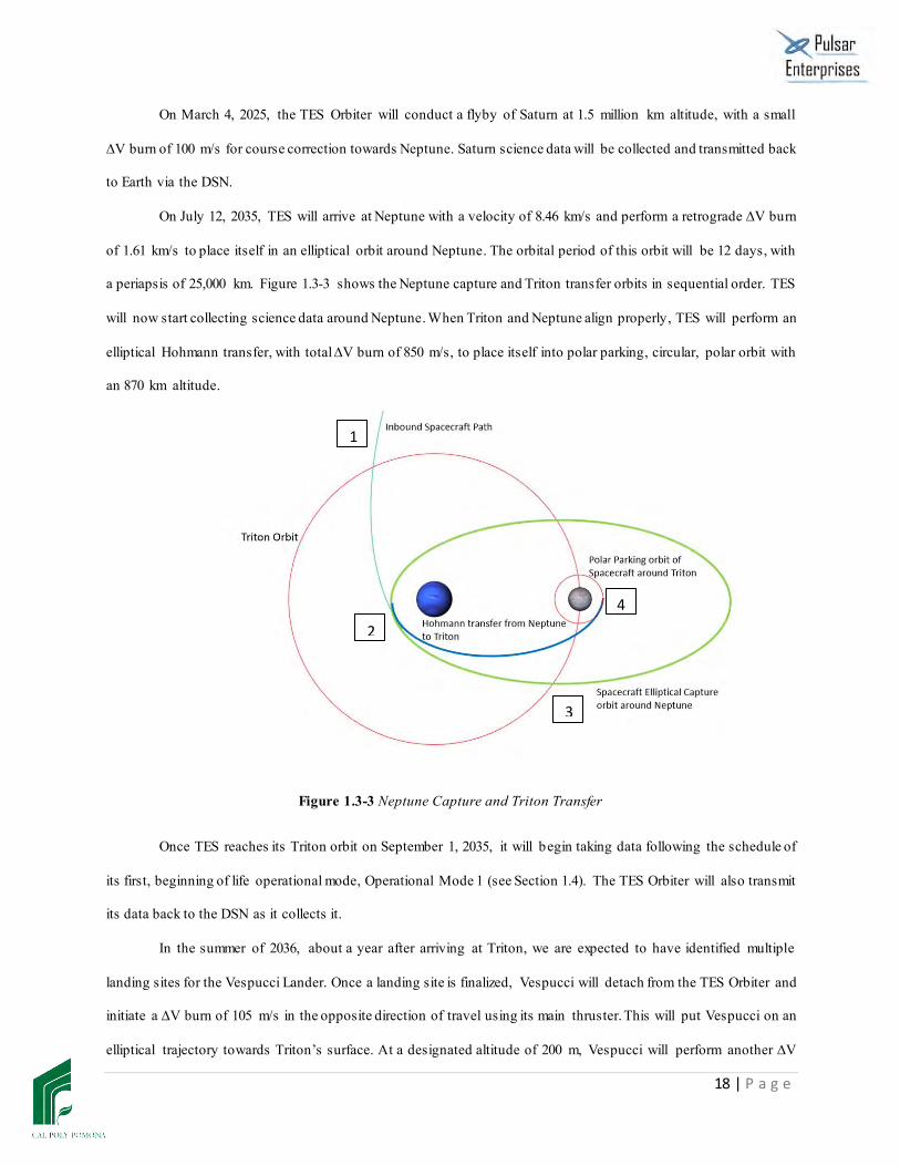
On March 4, 2025, the TES Orbiter will conduct a flyby of Saturn at 1.5 million km altitude, with a small
∆V burn of 100 m/s for course correction towards Neptune. Saturn science data will be collected and transmitted back
to Earth via the DSN.
On July 12, 2035, TES will arrive at Neptune with a velocity of 8.46 km/s and perform a retrograde ∆V burn
of 1.61 km/s to place itself in an elliptical orbit around Neptune. The orbital period of this orbit will be 12 days, with
a periapsis of 25,000 km. Figure 1.3-3 shows the Neptune capture and Triton transfer orbits in sequential order. TES
will now start collecting science data around Neptune. When Triton and Neptune align properly, TES will perform an
elliptical Hohmann transfer, with total ∆V burn of 850 m/s, to place itself into polar parking, circular, polar orbit with
an 870 km altitude.
Figure 1.3-3 Neptune Capture and Triton Transfer
Once TES reaches its Triton orbit on September 1, 2035, it will begin taking data following the schedule of
its first, beginning of life operational mode, Operational Mode 1 (see Section 1.4). The TES Orbiter will also transmit
its data back to the DSN as it collects it.
In the summer of 2036, about a year after arriving at Triton, we are expected to have identified multiple
landing sites for the Vespucci Lander. Once a landing site is finalized, Vespucci will detach from the TES Orbiter and
initiate a ∆V burn of 105 m/s in the opposite direction of travel using its main thruster. This will put Vespucci on an
elliptical trajectory towards Triton’s surface. At a designated altitude of 200 m, Vespucci will perform another ∆V
1.
2.
4
.
1
.
3
.

19 | P a g e
burn of 700 m/s to bring velocity to 5.00 m/s, relative to Triton. It will then be in free fall until it reaches 10 m, where
it will conduct its final ∆V burn of 17.5 m/s in an upward direction. The kinematic energy of Vespucci at the moment
of surface impact will be 0.055 J, which is well below NASA’s criteria of 100 J for spacecraft survival.[6] The descent
will take a total of 1.05 hours. Once Vespucci is on the surface, it will collect and transmit data for approximately 12
hours. Figure 1.3-4 presents a visual representation of the Vespucci Lander concept of operations.
Figure 1.3-4 Vespucci Lander Concept of Operations
Vespucci will continuously take data and transmit all necessary data back to TES when in view for 1.51 hours
per orbit, and will continue transmitting for each subsequent pass-over until all data has been transmitted or until
battery power ceases. Figure 1.3-5 shows the field of view between TES and Vespucci. TES will process, store, and
relay Vespucci’s data back to Earth.
Figure 1.3-5 Vespucci Lander Transmission Operations
870 km
3.33 hours
1.51 hours

20 | P a g e
On December 1, 2039, the science data collection will end, but the telecommunications system will continue
to transmit data via DSN. About a year before that, and as RTG power output continues to decay, the TES Orbiter will
no longer be able to operate multiple subsystems at the same time. Thus, it will enter Operational Mode 2 (see Section
1.4). The last year is dedicated solely to transmission. Finally, on December 1, 2040, all data transmission will cease.
The TES Orbiter will move into a graveyard orbit until the RTGs can no longer provide sufficient power to operate.
1.4 Operational Modes
During the various phases of the mission, different spacecraft modes must be implemented to efficiently
distribute power to the instruments and other components of the spacecraft. The different modes have been broken
down into two operational modes with two science modes each.
Each mode was chosen based on the spacecraft’s position in orbit, our DSN usage per day, and the available
power. The illumination period of our 4.84 hour orbit is 3.83 hours, leaving about 1.01 hours of eclipse period.
Throughout the life of the mission, we will continuously have 8 hours of DSN usage per day. However, RTG power
starts at 440 W at beginning of life (BOL), and at end of life (EOL), our RTG power is only 217 W. For these three
reasons (eclipse, DSN, power), two different operational modes are necessary.
Operational Mode 1 is implemented during the BOL of the mission. Within this mode, there are two science
modes. Since this is at BOL, we have enough RTG power to use all instruments at the same time. Science Mode 1
defines the use of all six science payloads aboard TES (see Section 2.2), while also simultaneously transmitting back
to Earth. Science Mode 1 is broken into two sections; the first section lasts 2.67 hours and is when TES collects and
transmits data at the same time. The second section lasts for 1.16 hours and only data is collected. Adding up both
these times leads to a total time of 3.83 hours for Science Mode 1, which is the illumination period of the orbit. Science
Mode 2 is implemented during the orbit’s eclipse period of 1.01 hours. In this mode, only the dust analyzer,
magnetometer, and radio science surveyor will be used. During the eclipse, the visible light camera, infrared
spectrometer, and ultraviolet spectrometer will not be as useful, so to save power, they will not be used. During the
1.01 hour eclipse period, 0.07 hours will be dedicated to engineering data to check the status of the spacecraft. The
rest will be used for data collection. Figure 1.4-1 shows a visual representation of our orbit’s illumination and eclipse
periods. Figure 1.4-2 shows Operational Mode 1, with Science Mode 1, Science Mode 2, transmission, and
engineering data times shown.

21 | P a g e
Figure 1.4-1 Illuminated vs Eclipse Orbital Periods
Figure 1.4-2 BOL Operations showing Science Modes 1 & 2 per Orbit

22 | P a g e
Near EOL, power must be allocated more carefully because of our RTG degradation. During this part of the
mission, TES will enter Operational Mode 2. There are also two science modes in this operational mode: Science
Mode 1E and Science Mode 2E. Due to less power being available, transmitting data and collecting data must be done
separately. This time, during the illumination period of TES’ orbit, it will spend 1.61 hours just transmitting data to
Earth. For the next 2.22 hours, TES will enter Science Mode 1E and operate all of its payload items at once. The
following eclipse period is the same at EOL as it was for BOL. TES will spend 0.94 hours in Science Mode 2E, using
only its dust analyzer, magnetometer, and radio science surveyor, and 0.07 hours doing engineering data. Figure 1.4 -
3 shows Operational Mode 2 at EOL.
Figure 1.4-3 EOL Operations showing Science Modes 1 & 2 per Orbit
During descent, Vespucci will operate its dust analyzer to receive additional atmospheric particle data and
its visible light camera to watch its descent. Once Vespucci is on the surface of Triton, it will begin full operation of
all of its payload items, including its cameras and spectrometers . Vespucci is designed to operate for 12 hours at
maximum power, which relates to at least two orbits made by TES. Vespucci will collect and transmit data to TES
simultaneously.
23 | P a g e
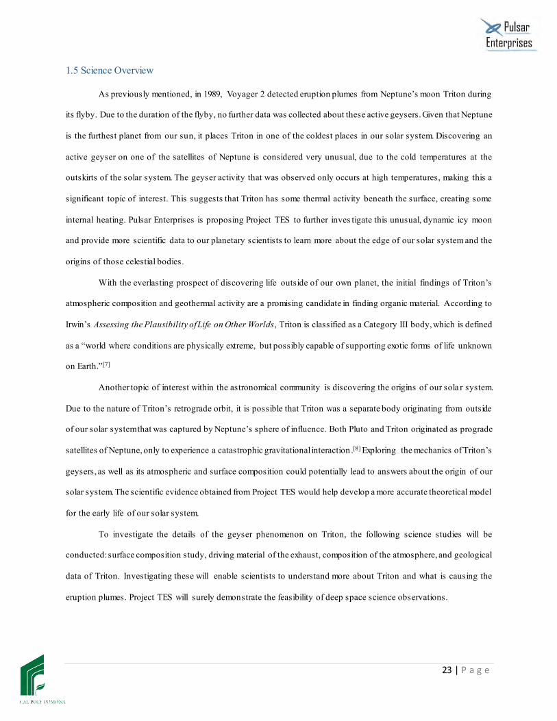
1.5 Science Overview
As previously mentioned, in 1989, Voyager 2 detected eruption plumes from Neptune’s moon Triton during
its flyby. Due to the duration of the flyby, no further data was collected about these active geysers. Given that Neptune
is the furthest planet from our sun, it places Triton in one of the coldest places in our solar system. Discovering an
active geyser on one of the satellites of Neptune is considered very unusual, due to the cold temperatures at the
outskirts of the solar system. The geyser activity that was observed only occurs at high temperatures, making this a
significant topic of interest. This suggests that Triton has some thermal activity beneath the surface, creating some
internal heating. Pulsar Enterprises is proposing Project TES to further inves tigate this unusual, dynamic icy moon
and provide more scientific data to our planetary scientists to learn more about the edge of our solar system and the
origins of those celestial bodies.
With the everlasting prospect of discovering life outside of our own planet, the initial findings of Triton’s
atmospheric composition and geothermal activity are a promising candidate in finding organic material. According to
Irwin’s Assessing the Plausibility of Life on Other Worlds, Triton is classified as a Category III body, which is defined
as a “world where conditions are physically extreme, but possibly capable of supporting exotic forms of life unknown
on Earth.”[7]
Another topic of interest within the astronomical community is discovering the origins of our sola r system.
Due to the nature of Triton’s retrograde orbit, it is possible that Triton was a separate body originating from outside
of our solar system that was captured by Neptune’s sphere of influence. Both Pluto and Triton originated as prograde
satellites of Neptune, only to experience a catastrophic gravitational interaction .[8] Exploring the mechanics of Triton’s
geysers, as well as its atmospheric and surface composition could potentially lead to answers about the origin of our
solar system. The scientific evidence obtained from Project TES would help develop a more accurate theoretical model
for the early life of our solar system.
To investigate the details of the geyser phenomenon on Triton, the following science studies will be
conducted: surface composition study, driving material of the exhaust, composition of the atmosphere, and geological
data of Triton. Investigating these will enable scientists to understand more about Triton and what is causing the
eruption plumes. Project TES will surely demonstrate the feasibility of deep space science observations.

24 | P a g e
1.6 Science Objectives
The primary observational target for this mission are the geysers on Triton’s surface in the region near its
south pole. Additional targets include the atmosphere of Triton and its surface.
For the active geysers on the surface, scientific measurements must be taken of both the gaseous exhaust and
the solid material that is expelled from the geyser to gain a clear understanding them. Pressure and volume density
measurements of the gaseous exhaust must be taken, as well as composition and particle size of the solid material in
the plume. These measurements will be taken remotely using TES, and directly with Vespucci as the geyser precipitate
falls upon its dust analyzer.
Triton’s entire surface must be fully mapped, with emphasis on its geyser region. This geological mapping
should include enough data to understand surface composition, surface history, mineral history, and thermal
characteristics. Some of the surface composition analysis should be performed in a clean area not affected by the
geyser zone or any nearby geyser plumes.
Regarding Triton’s atmosphere, measurements must be taken for the composition, pressure, temperature, and
density. These measurements will be taken from above the thermopause.
1.7 Primary Requirements
The project’s primary requirements are interpreted directly from the given RFPs from JPL and AIAA. Table
1.7-1 is a summary of the both RFPs’ primary requirements, showing their respective numbers and their condition.
These top-level requirements form the backbone of our mission planning and spacecraft architecture design.
Table 1.7-1 Primary Requirement Breakdown
RFP Req. # Requirement Description Required/Optional JPL T0.1 Provide data for mineral, surface history, and thermal mapping of
Triton’s geyser zone with a resolution of 10 m Required
JPL T0.1.1 Full surface mapping at 1 m resolution Optional JPL T0.2 Determine composition of the geyser zone surface in a clean area
not covered by geyser precipitation Required
JPL T1.1 System shall be capable of differentiating between areas of the geyser zone that are covered or not covered by geyser
precipitation
Required
JPL T1.2 System shall be capable of analyzing surface soils Required JPL T0.3 Determine the composition, particle size, and particle volume
density of the solid material released by Triton’s geysers Required
JPL T0.4 Determine the composition of the geyser-driving exhaust and its pressure and volume density in the eruption plume
Required

25 | P a g e
JPL T0.5 Determine the composition, temperature, pressure, and density of Triton’s atmosphere from 20 km above its thermopause to the
surface at 100 m intervals in altitude
Required
JPL T0.5.1 Map atmosphere 100 km above the surface at 10 m intervals Optional JPL T1.3 System shall have the capability to analyze the composition of a
trace atmosphere Required
JPL T0.6 Atmospheric measurements shall be made 75 km upwind of any geysers in the region or 40 km crosswind and outside the
periphery of the geyser region
Required
JPL T1.4 System shall be capable of orienting its instrumentation to avoid interference by geyser plumes
Required
JPL T0.7 Arrive at Triton by December 2035, completion of operations before December 2039 and data delivery by December 2040
Required
JPL T0.8 All scientific data shall be delivered to the Planetary Data System Required JPL T1.5 System must be capable of interfacing with the Deep Space Network Required JPL T1.6 Spacecraft shall be capable of using its instruments in deep interplanetary
space Required
JPL T0.9 System must be capable of performing science operations prior to arrival at Triton
Required
AIAA T0.10 System must be capable of launching aboard a currently available launch vehicle including SLS
Required
JPL T0.11 System shall abide by NASA’s planetary protection protocols Required JPL C0.1 Project cost cap is $5 billion Required JPL M0.1 Mission Concept Review is due the last half of March 2017 Required
AIAA M0.2 Preliminary Design Review is due the last half of May 2017 Required
1.8 Derived Requirements
Based on the primary requirements outlined above, derived requirements have been developed that specify
how the primary requirements shall be applied to our mission. Table 1.8-1 lists all derived requirements that drive the
design of each of our spacecraft’s subsystems. Although each subsystem has its own derived requirements, a full
requirements breakdown of every subsystem is beyond the scope of this report, so only top level derived requirements
that influence multiple subsystems have been included below in Table 1.8-1.
Table 1.8-1 Derived Requirements Breakdown
RFP Req. # Requirement Description Required/Optional JPL T1.1 System shall be capable of differentiating between areas of the geyser zone that
are covered or not covered by geyser precipitation Required
JPL T1.2 System shall be capable of analyzing surface soils Required JPL T1.3 System shall have the capability to analyze the composition of a trace atmosphere Required JPL T1.4 System shall be capable of orienting its instrumentation to avoid interference by
geyser plumes Required
JPL T1.5 System must be capable of interfacing with the Deep Space Network Required JPL T1.6 Spacecraft shall be capable of using its instruments in deep interplanetary space Required

26 | P a g e
2.0 Scientific Payload
2.1 Payload Overview
Our payload suite consists of ten science instruments. The payload items tie directly to our JPL RFP, and to
complete our science objectives, the correct instrumentation for each requirement had to be selecte d. When
determining which instruments to use, three main design drivers were specified: mass, power, and ground resolution.
Furthermore, each requirement listed in the RFP was decomposed into basic objectives and categorized with an
accompanying type of instrument.
Our analyses identified that there were six specific types of payloads that were essential to the completion of
the requirements listed in the RFP. These included visible light cameras, infrared spectrometers, ultraviolet
spectrometers, visible and infrared mapping spectrometers, particle and dust analyzers, and radio science and
magnetometer experiments. As we conducted further trade studies, however, it became clear that to minimize mass
and power usage and to increase the simplicity and efficiency of our system, our goals could be accomplished by
merging two redundant instruments together by using only five of the six different types of payload. In this case, we
decided to omit the infrared spectrometer and instead rely on our visible and infrared mapping spectrometers to cover
this measurement.
All instruments will be produced specifically for this mission, with their specifications catered towards
efficiency and quality. To correctly estimate the mass, power, resolution, data rate, and tempera ture limits of each of
our instruments, the following trade study was conducted. First, the equivalent instruments from previous space
missions were compiled based on year, and their mass and power properties were listed. [9-28] The properties of each
instrument were then plotted on a line graph versus time to develop a rough trend of how the technology changes over
time (very large outliers were omitted). From here, a more detailed trend line was applied to the data points and
projected forward to our expected production year of 2022. Following the trend line, we obtained a value for the mass,
power, resolution, and data rates for our new instruments. The mass, power, and resolution trend lines were then
overlaid onto each other and onto one plot to determine the point at which they intersect. This intersection point helped
verify that all the new values for our instruments agreed with each other so that no one value was inflated or
exaggerated. It also confirmed that the trend lines were accurate and pointed to the same conclusion. In addition, using
this method, we can classify all our payload items as a Technology Readiness Level of 9, based on NASA’s definitions,
since we are just improving their efficiencies from over time.[29]

27 | P a g e
The instruments we are using are distinguished between our TES Orbiter and our Vespucci Lander payloads.
TES consists of six instruments: a visible light camera, an infrared spectrometer, an ultraviolet spectrometer, a dust
analyzer, a radio science instrument, and a magnetometer. Each instrument satisfies a particular requirement in our
compliance matrix, while also providing some useful additional data not specifically requested in the RFP. Vespucci
consists of four instruments: a visible light camera identical to the one on the orbiter, a dust analyzer, a ground
penetrating radar, and a multi-purpose infrared spectrometer capable of looking at Triton’s surface up-close. With
TES and Vespucci combined, there is a total of ten scientific instruments. Each instrument is listed below a nd further
elaborated upon.
2.2 TES Orbiter Payloads
2.2.1 Visible Light Camera, “HRCC”
Our main instrument for taking pictures of the surface of Triton is our visible light camera placed on TES,
abbreviated HRCC, for High-Resolution Color Camera. It is a panchromatic camera with a resolution of 2048 x 2048
pixels, a mass of 2.5 kg, and a power usage of 4 W. This camera will give us the clearest pictures of Triton ever taken.
It will satisfy requirements T0.1 and T0.2 as listed in our compliance matrix. This camera will take pictures at an
altitude of 870 km above the surface of Triton and is the main camera that will be used for mapping the surface, taking
pictures, and identifying potential landing sites for our lander.
2.2.2 Visible and Infrared Mapping Spectrometer, “VIS”
There will be one visible and infrared mapping spectrometer, VIS, on TES. Its main purpose is to analyze
the atmosphere and geysers of Triton and determine their composition, density, temperature, and in the case of the
geysers, the driving force and exhaust material. It is also a visible mapping spectrometer to analyze the composition
of the surface materials. It will operate within the spectral ranges of 300-2900 nm and 5800-50000 nm, which is in
the visible range of the spectrum as well as the mid/far range of the infrared spectrum. This instrument will specifically
satisfy requirements T0.1, T0.2, T1.1, T1.2, T0.3, T0.5, T1.3, and T0.6 in our compliance matrix. VIS has a mass of
8 kg and a power usage of 15 W.
2.2.3 Ultraviolet Spectrometer, “UVS”
The TES also contains one ultraviolet spectrometer, which will be used to conduct further, detailed analyses
of Triton’s trace atmosphere. More specifically, it will be used to understand the density, temperature, energy, and
composition of the particles in the atmosphere. It will also be used to study the composition of the surface and geyser

28 | P a g e
plume material. It operates in the spectral range of 50-195 nm, with a mass of 5.5 kg and a power usage of 6 W. Our
UVS satisfies requirements T0.4, T0.5, T0.6, T1.3, and T1.4 as listed in our compliance matrix.
2.2.4 Dust Analyzer, “TDA”
There will be two distinct direct sensors in our system. Both are particle analyzers, but take measurements
differently, as one is placed on TES and one is on Vespucci. This first dust analyzer is called the TDA, or Triton Dust
Analyzer, and is placed on TES. It has a mass of 1 kg and a power usage of 3 W. As TES orbits through the trace
atmosphere of Triton, some of the particles will be caught in this instrument . TDA will then analyze the energy, mass,
and speed of the particles caught in its sensors. It is our only direct sensor on our orbiter and will help us better
understand the properties of Triton’s atmosphere. TDA satisfies requirements T0.5 and T1.3 in the compliance matrix.
2.2.5 Radio Science, “RAT”
The TES Orbiter also has a radio science instrument onboard, called RAT, or Radio Atmospheric Testing. It
will study the atmosphere of Triton with radio waves. This will give us additional data on the profile of the atmosphere,
which can then be correlated with the data from the ultraviolet and infrared spectrometers to increase the accuracy of
our findings. RAT has a mass of 4 kg and a peak power usage of 7.5 W, and will help satisfy requirements T0.5, T0.6,
T1.3, and T1.4.
2.2.6 Magnetometer, “MAGIC”
The final scientific instrument aboard our orbiter is a magnetometer, named MAGIC, standing for Magnetic
Investigator and Characterizer. MAGIC will allow us to study the anomalous magnetic field of Triton and potentially
the magnetic field of Neptune as well. Although this objective is not explicitly stated in the RFP, it would be interesting
to learn more about Triton. MAGIC has a low mass of just 3 kg and low power usage of 3 W, thus, the tradeoff for
additional useful data is not severe at all. The only consideration when choosing to include this payload item was the
fact that a potentially heavy and long boom would be necessary. The boom for the magnetometer has a mass of 2 kg .
2.3 Vespucci Lander Payloads
2.3.1 Visible Light Camera, “HRCC”
This is the same camera that is also placed on the TES orbiter. When placed on Vespucci, HRCC will help
us fulfill requirement T0.1, as it will give us more close-up, high-resolution pictures of the surface. After landing,
Vespucci will first take a 360 panorama picture of Triton’s surface.

29 | P a g e
2.3.2 Dust Analyzer, “LDA”
The secondary particle analyzer on Vespucci will study the particles and precipitate from the geyser plumes .
LDA, or Local Dust Analyzer, can measure the mass, speed, and energy of the particles that fall on it from the exhaust
material. It has a mass of 1.5 kg and a power usage of 4 W. This is the sole direct sensor on our Vespucci Lander and
will help us further understand the composition of the material jettisoning from the geysers on the surface of Triton.
LDA satisfies requirements T0.2 and T0.4.
2.3.3 Subsurface Surveyor, “Triple-S”
Also on Vespucci is a ground penetrating radar, called Triple-S, for Subsurface Surveyor. It will use radio
waves to study the surface and subsurface of Triton. More specifically, it will help us better understand the
composition of the surface soil, the soil underneath, and any potential geyser precipitate resting on the surface. It has
a mass of 3 kg and a power usage of 5 W. The instrument satisfies requirement T0.1, T0.2, T0.3, T1.1, and T1.2.
2.3.4 Surface Infrared Spectrometer, “LIS”
The final instrument on our Vespucci Lander is another infrared spectrometer, called LIS, standing for Lander
Infrared Spectrometer. It operates in the spectral ranges of 5000-29000 nm. This instrument will study surface dust
and plume precipitate up-close, and will provide very accurate data because of how close it is to the sample being
studied. Much of our data from Vespucci will come from this instrument. LIS has a mass of 2 kg and a power usage
of 5 W. It will satisfy requirements T0.1, T0.2, T0.3, T1.1, and T1.2 in the compliance matrix.
2.4 Payload Summary
The payloads for each spacecraft are tabulated below, showing mass, power, and various other propert ies of
each instrument. The totals are shown at the bottom of the table. Table 2.4-1 below shows the TES Orbiter instruments,
and Table 2.4-2 shows the instruments for our Vespucci Lander.
Table 2.4-1 TES Payload (Orbiter)
Instrument Mass [kg]
Peak Power [W]
Ground Resolution [m/pixel]
Resolution [pixel x pixel]
FOV [mrad x mrad]
Max Data Date
[kbps]
Design Life
[years]
TRL
HRCC 2.5 4 7 2048 x 2048 16.5 10066.33 25 9 UVS 5.5 6 8 1024 x 128 9.4 6.43 25 9 VIS 8 15 15 256 x 256 4.4 0.85 25 9 TDA 1 3 - - - 2.22 25 9 RAT 4 7.5 - - 3141.59 0.80 25 9
MAGIC 3 3 - - Point Source 4.05 25 9 Total 24 38.5

30 | P a g e
Table 2.4-2 Vespucci Payload (Lander)
Instrument Mass [kg]
Peak Power [W]
Ground Resolution [m/pixel]
Resolution [pixel x pixel]
FOV [mrad x
mrad]
Max Data Date
[kbps]
Design Life
[years]
TRL
HRCC 2.5 4 7 2048 x 2048 16.5 10066.33 25 9 Triple-S 3 5 - - 3141.59 1.08 20 9
LIS 2 5 5x10⁻⁶ (0.2 m above ground)
256 x 256 0.366 0.85 20 9
LDA 1.5 4 - - - 0.08 20 9 Total 9 18
2.5 Scientific Payload Operations Scenario
As mentioned above in Section 1.4, there are two operational modes for TES, with two science modes each.
In September of 2035, upon Triton arrival, main science operations will begin. However, prior to arrival at Neptune
during cruise, basic science operations will still be done. For example, there are opportunities to begin payload
operations during the Saturn flyby, Neptune capture, or asteroid belt flyby. During our orbit’s illumination period of
3.83 hours, the HRCC will continuously take photos of the surface of Triton (while it is exposed to sunlight), while
the VIS and UVS will operate in tandem in order to analyze the composition, density, and pressure of the atmosphere,
and also study the geyser plume material. The imaging instruments will also be responsible for providing potential
landing spots for the Vespucci Lander. However, during eclipse periods, which last approximately 1.01 hours per
orbit, the HRCC, VIS, and UVS shall be made idle. Here further studies will be conducted by TDA, RAT, and MAGIC.
While it is an analysis of a trace atmosphere at an 870-km altitude, the TDA shall analyze the properties of any particles
its sensors can catch; meanwhile, MAGIC shall continuously study magnetic fields and RAT shall collect atmospheric
data.
The Vespucci Lander shall provide another set of data about Triton. Each of the instruments will contribute
in their own ways to form a detailed model of Triton’s surface. For example, LDA will give a more accurate reading
of the composition of the materials projected from the geysers. Meanwhile, Triple-S will analyze the soil materials
and geyser components that rest on and beneath the surface. Given the low power requirements of the four instruments
on the lander, each can remain fully operational for as long as there is power available to run the lander (approximately
12 hours). Vespucci will continuously take data. In terms of transmitting data to the Planetary Data System (PDS),

31 | P a g e
there will be about a 1.51 hour window when TES and Vespucci will be in direct contact with each other, allowing
the lander’s data to be transmitted to the orbiter, and eventually relayed back to the PDS.
The data collected from the instruments of TES shall continuously be transmitted back to the PDS from the
time the instruments are activated until they are decommissioned in December 2040 – totaling up to just over 5 years
of analysis of Triton. However, each instrument shall cease its operation one year before decommission in December
2039, at which time the disposal process shall commence.
2.6 Science Traceability Matrix
The payload instruments to be used in the spacecraft will be carefully chosen to fulfill each of the science
requirements given in the RFP. Table 2.6-1 gives a layout of each science objective, as well as the corresponding
goals, instrument(s) and purpose of said instrument(s) in relation to how it achieves the objectives.
Table 2.6-1 Science Traceability Matrix for Objectives and Instruments
Science Objective Required Ref. # Goals Instrument Geyser zone surface shall be fully
mapped to a ground resolution of 10 meters
T0.1 T0.1.1
Fully mapped to a ground resolution of 1
meter
HRCC VIS
Triple-S LIS
Composition of geyser zone not covered in precipitate shall be studied
T0.2 T1.1 T1.2
- HRCC VIS LDA
Triple-S LIS
Measurements shall be taken for composition, particle size, and particle volume density of geyser solid material
T0.3
- VIS Triple-S
LIS Composition of geyser exhaust and
pressure and volume density shall be taken
T0.4 - UVS LDA
Composition, temperature, pressure, and density of atmosphere shall be taken at 20
km above thermopause at 100 m intervals; 75 km upwind and 40 km
crosswind of geysers
T0.5 T0.5.1 T1.3 T0.6
100 km altitude at 10 m intervals
VIS UVS TDA RAT
3.0 Mission Overview and Implementation
3.1 Mass Budget
Initial mass estimates were performed using Brown’s estimation criteria.[30] As our design process progressed,
each subsystem was further refined to get more accurate numbers. Finally, the exact mass values for each subsystem
32 | P a g e
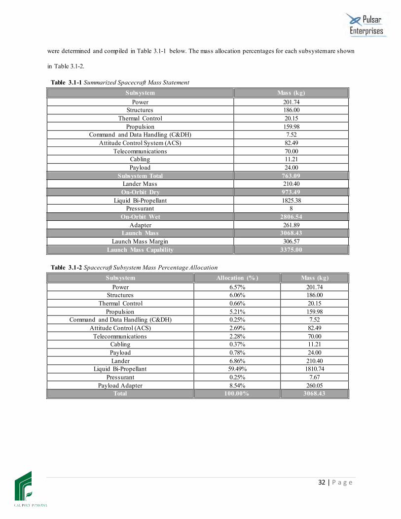
were determined and compiled in Table 3.1-1 below. The mass allocation percentages for each subsystem are shown
in Table 3.1-2.
Table 3.1-1 Summarized Spacecraft Mass Statement Subsystem Mass (kg)
Power 201.74 Structures 186.00
Thermal Control 20.15 Propulsion 159.98
Command and Data Handling (C&DH) 7.52 Attitude Control System (ACS) 82.49
Telecommunications 70.00 Cabling 11.21 Payload 24.00
Subsystem Total 763.09 Lander Mass 210.40 On-Orbit Dry 973.49
Liquid Bi-Propellant 1825.38 Pressurant 8
On-Orbit Wet 2806.54 Adapter 261.89
Launch Mass 3068.43 Launch Mass Margin 306.57
Launch Mass Capability 3375.00
Table 3.1-2 Spacecraft Subsystem Mass Percentage Allocation Subsystem Allocation (% ) Mass (kg)
Power 6.57% 201.74 Structures 6.06% 186.00
Thermal Control 0.66% 20.15 Propulsion 5.21% 159.98
Command and Data Handling (C&DH) 0.25% 7.52 Attitude Control (ACS) 2.69% 82.49
Telecommunications 2.28% 70.00 Cabling 0.37% 11.21 Payload 0.78% 24.00 Lander 6.86% 210.40
Liquid Bi-Propellant 59.49% 1810.74 Pressurant 0.25% 7.67
Payload Adapter 8.54% 260.05 Total 100.00% 3068.43

33 | P a g e
3.2 Power Budget
Similar to the mass budget, initial power estimates were performed using Brown’s estimation criteria. [30]
After many iterations, final power values were determined for each subsystem. The final power statement is shown in
Table 3.2-1, and the allocation percentages for each subsystem is in Table 3.2-2.
Table 3.2-1 Spacecraft Power Statement Subsystem Power (W)
Power 45.00 Structures 0.00
Thermal Control 1.50 Propulsion 76.58
Command and Data Handling (C&DH) 27.50 Attitude Control System (ACS) 108.24
Telecommunications 62.00 Cabling 14.00
Total 344.52 Payload 38.50
Total On-Orbit Dry 373.32 BOL Margin 66.68 EOL Margin -156.32
MMRTG Power BOL 440 MMRTG Power EOL 217
Table 3.2-2 Spacecraft Subsystem Power Percentage Allocation Subsystem Allocation (% ) Power (W)
Power 12.05% 45.00 Structures 0.00% 0.00
Thermal Control 0.40% 1.50 Propulsion 20.51% 76.58
Command and Data Handling (C&DH) 7.37% 27.50 Attitude Control System (ACS) 28.99% 108.24
Telecom 16.61% 62.00 Cabling 3.75% 14.00 Payload 10.31% 38.50
Total 100.00% 373.32
3.3 Complete Mass and Power Statement
The complete, detailed mass and power statement is shown in Table 3.3-1. Each subsection is broken down
and the corresponding mass and power for each component is shown.

34 | P a g e
Table 3.3-1 Complete System Mass and Power Statement
Components Mass (kg) Power (W)
Batteries 0 0.00(4) MMRTGs with Attachment Hardware 174.4 0.00
Power Regulatory Unit, Power Distribution unit, Shunts 25.14 45.00
Bus Mass 365.00 0.00
Heat Pipes 9.99 0.00(2) Radiators 7.88 0.00
(3) Thermal Switches 0.06 1.00(16) RHUs 0.64 0.00
Multi-Layers Insulation 1.49 0.00(3) Temperature Sensors 0.09 0.50
Fill and Drain Valve 0.226 0.00Fuel Tank 21.48 0.00
Oxidizer Tank 13.86 0.00Pressurant Tank 36.54 0.00
Mounting Hardware 63.75 0.00Pressure Transducer 0.68 6.00Temperature Sensor 1.36 3.00
Open Pyro Valve 1.23 0.00Closed Pyro Valve 1.08 0.00
Solenoid Valve 2.04 19.16Latching Valve (No Relief) 1.02 3.00Pressure Regulator w/Filter 2.08 0.00
Check Valve 1.09 0.00Relief Valve 1.70 0.00
Flow Balance Orifice 0.46 0.00System Filter 0.57 0.00
Main Thruster 5.40 45.00Piping 12.68 0.00
C&DH Processor Card 0.15 5.00Solid State Recorder (SSR) Card 7.10 17.00
Instrument Interface Card 0.07 2.50Critical Command Decoder (CCD) on Uplink Card 0.10 2.50
Downlink Formatter on Downlink Card 0.10 0.50
ACS Thrusters 3.96 27.28Reaction Wheel 34.00 28.00
Magnetic Torque Rod 11.20 7.91Gyroscopic Controls 13.50 25.00
Star Trackers 19.41 19.80Sun Trackers 0.38 0.25
Electra Radio and UHF Antenna 7.00 10.00Telecom Panel 20.00 0.00
Antenna (High Gain and Low Gain) 30.00 0.00SDST 10.00 2.00
(2) SSPA 3.00 50.00
Electrical Cabling 11.21 14.00
Visible Light Camera 2.50 4.00UV Spectrometer 5.50 6.00
Visible/Infrared Mapping 8.00 15.00Particle Energy Analyzer Spectrometer (PEAS) 1.00 3.00
Magnetometer 3.00 3.00Radio & Plasma Wave Science 4.00 7.50
Power Subsystem 22.00 23.00Structures Subsystem 21.00 0.00
Thermal Control Subsystem 5.00 65.00Propulsion Subsystem 33.00 2.00
Command and Data Subsystem 8.00 40.00Attitude Control Subsystem 19.00 47.00
Telecomunications Subsystem 15.00 54.00Cabling Subsystem 7.00 2.00
Payload: Visible Light Camera 2.50 4.00Payload: Subsurface Surveyor 3.00 5.00Payload: Surface Spectrometer 2.00 5.00
Payload: Dust Analyzer 1.50 4.00Monopropellant 70.90 0.00
Cold Gas Proppellant 0.50 0.00
Liquid Bi-Propellant 1825.38 0.00Pressurant 7.67 0.00
Adapter 261.89 0.00
Cabling Subsystem
Payload
Lander
Thermal Control Subsystem
Propulsion Subsystem
Command and Data Subsystem
Attitude Control Subsystem
Telecommunications Subsystem
Propellent
Launch Adapter
Power Subsystem
Structures Subsystem

35 | P a g e
3.4 Spacecraft Diagrams
As mentioned on the concept of operations, the spacecraft will be in four different configurations during its mission. The first configuration is during the launch phase of the spacecraft. The s pacecraft will be stowed and mounted on the payload adapter. Figures
3.4-1 to 3.4-4 show the 3-view drawing along with the isometric view of the spacecraft with its fairing for the first two figures, and without it for the last two.
Figure 3.4-1 Isometric View of Stowed TES in Fairing Figure 3.4-2 Front View of Stowed TES in Fairing Figure 3.4-3 Front View of Stowed TES on Payload Adapter Figure 3.4-4 Top View of Stowed TES
Once the launch vehicle’s fuel is depleted, the spacecraft will jettison off the launch vehicle, and the spacecraft is shown below with the upper stage in Figures 3.4-5 to 3.4-8.
Figure 3.4-5 Isometric View of TES Upper Stage Configuration Figure 3.4-6 Front View of TES Upper Stage Configuration Figure 3.4-7 Back View of TES Upper Stage Configuration Figure 3.4-8 Top View of TES Upper Stage Configuration
7 m
2 m
19.1 m
8.4 m

36 | P a g e
After the solid motor upper stage completes its burn, the upper stage adapter is jettisoned off of the spacecraft and the stowed spacecraft in transit to Neptune is shown on Figure 3.4-9 to 3.4-12.
Figure 3.4-9 Isometric View of TES Upper Stage Jettisoned Figure 3.4-10 Front View of TES Upper Stage Jettisoned Figure 3.4-11 Back View of TES Upper Stage Jettisoned Figure 3.4-12 Top View of TES Upper Stage Jettisoned
When the spacecraft arrives at Triton, the lander is jettisoned off the spacecraft and the magnetometer boom is fully deployed shown on Figure 3.4-13 to 3.4-16.
Figure 3.4-13 Isometric View of TES Deployed Figure 3.4-14 Front View of TES Deployed Figure 3.4-15 Back View of TES Deployed Figure 3.4-16 Top View of TES Deployed
5 m
2 m
4 m
2 m
14 m

37 | P a g e
3.5 Lander Diagrams
When Vespucci is released from TES, all systems are stowed. 3-view drawings are shown in Figures 3.5-1 to 3.5-3. The various instruments are highlighted.
Figure 3.5-1 Isometric View of the Vespucci Stowed Configuration Figure 3.5-2 Side View of the Vespucci Stowed Configuration Figure 3.5-3 Top View of the Vespucci Stowed Configuration
Once Vespucci landed on the surface of Triton, HRCC will rise from the lander to take a 360 degree panorama picture. 3-view drawings are shown below on Figures 3.5-4 to 3.5-6.
Figure 3.5-4 Isometric View of the Vespucci Deployed Figure 3.5-5 Side View of the Vespucci Deployed Figure 3.5-6 Top View of the Vespucci Deployed
2 m
1 m
4 m
2 m

38 | P a g e
4.0 Mission Trajectory
4.1 Launch Vehicle Selection
The launch vehicle issued by the AIAA RFP is the Space Launch System (SLS). For performance analysis
purposes, a launch vehicle trade study was conducted shown below in Table 4.1-1. The launch vehicles in comparison
are readily available or currently in development. The payload capacity to certain planets are shown. Also, the size of
the payload fairing for each launch vehicle is included to portray the similarities between them. The cost per launch
for the current launch vehicles are estimated based on previous missions, while the SLS is estimated similar to the
Saturn V launch vehicle due to its size and launch capability.
Table 4.1-1 Launch Vehicle Trade Study
Launch Vehicle
LEO (kg)
GTO (kg)
Mars (kg)
Jupiter (kg)
Saturn (kg)
Fairing Diameter
(m)
Fairing Length
(m)
Cost ($M in 2016)
Falcon Heavy 54400 22200 13600 4080 0 5.2 13.1 135 SLS Block 1B 105000 50000 30000 9000 0 8.4 19.1 1269 Delta IV Heavy 28790 14220 8571 2571 0 5 19.1 435
Ariane V 21000 10050 4500 1800 0 5.4 18.1 220
The SLS variant that this mission will utilize is the SLS Block 1B. It features 2 solid rocket boosters, four
RS-25 liquid propellant engines for the core stage, the Exploration Upper Stage (EUS) with four RL10 liquid
propellant engines, and outputting at liftoff thrust of 8.8 million pounds.[31] The SLS Block 2, which is identical to the
Block 1B except for advanced rocket boosters, an upper stage, and a larger payload fairing, is shown in an exploded
view below in Figure 4.1-1. A figure of Block 1B was unavailable, so the next closest SLS was used.
Figure 4.1-1 Space Launch System Block 2 Exploded View

39 | P a g e
The payload capacities at various C3 capabilities were obtained through the launch vehicle payload planner
guides. None of the sources contained capabilities past Jupiter, therefore trends to Saturn had to be independently
developed. Figure 4.1-2 is shown below to prove that the SLS is currently the most capable of launch vehicles for
deep space interplanetary travel.
Figure 4.1-2 Launch Vehicle Payload Capacity versus C3 Capability
4.2 Upper Stage Selection & Integration
In Figure 4.1-2 shown above, all the launch vehicles do not reach past a C3 of 140 km2/s2. This is a big
problem because the trajectory analysis done in Section 4.3 allocated a C3 of 143 km2/s2. Thus, it was decided to
implement an additional upper stage or kick motor.
Referencing the SLS Payload Planner Guide [31], the payload fairing does not have any restrictions on
additional stages inside the fairing bay. With that noted, upper stages were explored to increase the p ayload capacity
for this mission. The dimensions, availability, cost, and C3 capability were taken into consideration for assessing the
most ideal choice for this mission.
Liquid bipropellant upper stages such as Centaur[32], the DCSS[33], and the EUS[34] were originally considered,
but all had a large excess of C3 capability, on top of a high cost. To save on cost and stay within a reasonable C3
capability increase, a kick motor was considered.
The Orbital ATK Star 37 XFP was chosen based on its availability and experience in prior space missions.[35]
The Orbital ATK Star XFP addition increases the overall SLS C3 capability to 160 km2/s2 and increases the payload

40 | P a g e
capability at a C3 of 143 km2/s2 to 3375 kg. This new payload capability will act as the launch mass capability to
determine our launch margin.
To integrate the payload and upper stage into the SLS payload fairing, two different payload attach fittings
were implemented. One of the fittings connected the SLS to the payload directly, while the othe r fitting attached the
Thiokol to the payload. The two fittings overlap each other when connecting to the payload and the Star 37 resides
inside the larger payload attach fitting. Figure 4.2-1 portrays the Thiokol integration into the payload configuration .
Figure 4.2-1 Orbital ATK Star 37 XFP Upper Stage Kick Motor Integration
4.3 Mission Trajectory Optimization
The importance of mission trajectory selection cannot be overstated. The trajectory that a spacecraft takes
over its mission lifetime determines the spacecraft’s fuel needs, time of flight, lifetime environmental conditions, and
constraints of possible launch vehicles and windows that could accommodate such a mission. The most important
constraint is the spacecraft mass, therefore, it is important to put a great amount of effort into trajectory selection and
optimization. In our case, arrival date was also a prominent constraint.
It is required that this mission reach Triton by the end of 2035. Given that initial planning for th is mission
began in late 2016, which leaves 19 years for mission conception, development, production, launch, and flight. A
typical low energy transfer trajectory for a spacecraft flying between the Earth and Triton would take just over 30
years to reach Triton. The 19-year time constraint requires a reduced production time and flight time. It would be
expensive in terms of labor costs, but by shaving time off production, we can lengthen the time of flight, decrease the
Orbital ATK Star 37 XFP
SLS Payload Adapter
Star 37 XFP Payload Adapter
Vespucci
TES

41 | P a g e
fuel costs for our mission, and increase the allowable spacecraft mass. Running under an accelerated production
schedule of 5 years, the estimated time that launch would occur is 2022. That gives us a flight time of 13 years.
Neptune has a low synodic period with Earth, just over a year. However, with the shortened flight time, any
feasible trajectory between the Earth and Neptune’s sphere of influence will likely need to be assisted by one of the
outer planets. Jupiter and Saturn have very large masses and good secondary scientific potential for flyby observations,
but both have larger synodic periods than Neptune, which will decrease the number of flyby opportunities that will be
possible. With these low number of flyby opportunities, missing our launch window will likely have a devastating
effect on the mission’s timetable, so alternative backup trajectories will also likely have to be selected.
It was important to analyze many different trajectory options, and have a tool that can generate plausible
trajectories quickly. We opted to utilize a genetic algorithm. Genetic algorithms are a good way to quickly generate
many different possible trajectories and down-select to the most optimum trajectory. However, there are several
downsides to using a genetic algorithm for this purpose. They tend to be good a t inducing artificial creativity by using
a random number generator to create slight alterations to a plausible solution, but they usually do not converge on the
same optimum solution every single time. Also, because a genetic algorithm depends on a random number generator
to generate new plausible solutions they tend to not analyze the full range of possibilities. Therefore, it may take
running a genetic algorithm many times to solve for a fully optimal solution.
The tool used was Trajectory Optimization Tool v2, developed by Adam Harden and published through
GitHub.[36] This tool uses the J2000 ephemeris and a Lambert Solver to generate possible interplanetary trajectories.
The tool allows the user to select an order of interplanetary flyby targets, time limits, and select weighting values for
solution fitness calculation. Solutions are selected based on their C3, flyby ΔV, and sphere of influence relative arrival
velocity. The output is a text file with launch, flyby, and arrival times, ΔV requirements, an d orbital elements for each
leg of the mission plan.
To find the true optimum solution, at least 150 runs were conducted. The algorithm was run with many
different planetary flyby sequences to see what effects each flyby opportunity had on the overall trajectory
performance. For each input flyby sequence, the algorithm was run multiple times to account for the inaccuracy of the
genetic algorithm. Using this method, 43 unique plausible trajectories were generated. The next step was to further
down select these partially optimized trajectory solutions. All solutions that required a launch before 2022 were

42 | P a g e
immediately discounted from consideration. The rest of the solutions were then analyzed in terms of arrival date at
Neptune’s sphere of influence and the mass requirements that each solution would impose on the mission.
To find the mass requirements imposed on the mission, the launch capability of the SLS Block 1B, the
required C3 of the solution, the required interplanetary ΔV, and the sphere of influence excess arrival velocity were
all combined using Tsiolkovky’s rocket equation to calculate the maximum spacecraft mass that could arrive at Triton.
This was a measure of effectiveness that we referred to as “deliverable mass to Triton”, and it was the main measure
used to down-select to our final trajectory solution. In Figure 4.3-1 below, each trajectory solution is represented by a
single data point.
Figure 4.3-1 Deliverable Mass Trade Study
The data points are color coded based on the order of planetary bodies used as a flyby opportunity. The
horizontal axis represents the arrival date at Neptune’s sphere of influence. The vertical axis represents our deliverable
mass to Triton on a logarithmic scale. As can be seen, most of our trajectory solutions are woefully incapable of
delivering a reasonably sized spacecraft to Triton. We can get a better look at our trajectory options by eliminating
any solution that cannot deliver at least 1 kilogram of mass to Triton.
Figure 4.3-2 shows how the revision drastically removes most of our plausible trajectories. From 43 plausible
trajectories, we have down selected to 8 possible trajectories. Most of these trajectories involve flybys of Saturn and

43 | P a g e
Jupiter. But this plot does not represent the time constraints on the mission. Figure 4.3-3 implements the 2035 deadline,
represented below by the red line, and the estimated dry mass of our spacecraft, represented by the purple line below.
Figure 4.3-2 Revised Deliverable Mass Trade Study with Only Masses 1 kg And Above
Figure 4.3-3 Final Revision of Deliverable Mass Trade Study

44 | P a g e
Following this criteria, we are left with only one trajectory solution which meets all our requirements.
Although the solutions to the right of the plot do not meet the arrival deadline requirements, they do represent several
plausible backup trajectories that have similar mass requirements if our program misses their original launch window.
Figure 4.3-4 shows the final trajectory for our system.
Figure 4.3-4 Visual Representation of Chosen Earth-Saturn-Neptune Trajectory
The trajectory launches from Earth in April 2022, flies by Saturn in March 2025, and arrives at Neptune’s
sphere of influence in July 2035. Due to the time constraints of the mission, our spacecraft uses highly elliptical orbits
to travel to Neptune at a very high speed similar to outer-planetary missions. We were fortunate that there was an ideal
flyby opportunity with Saturn during this launch flight period, as many other planets that could be used for a slingshot
maneuver were not in favorable positions to give us flyby chances.
4.4 Mission Trajectory
This mission can be broken up into the following segments: launch, departure from Earth, transfer to Saturn,
flyby through the Saturnian system, transfer to Neptune, capture around Neptune, phasing orbit around Neptune,
transfer to Triton, capture around Triton, and parking orbit around Triton. While this is a low number of maneuvers
for an interplanetary mission of this scale, this concept of operations was chosen to minimize flight time to meet our
strict flight time requirements, and to limit the number of unique environments that our spacecraft would have to

45 | P a g e
survive in. An overview of the transfer developed in the Trajectory Optimization Tool in MATLAB is shown in Figure
4.4-1.
Figure 4.4-1 Overview of Mission Trajectory
Launch will be handled by the SLS Block 1B. The spacecraft will take off from Cape Canaveral on April
12th, 2022, and be lifted onto a transfer trajectory towards Saturn with a C3 of 143.46 𝑘𝑚3/𝑠2. To achieve this, the
full lifting power of the SLS Block 1B cargo variant will be used in conjunction with an extra solid propellant kick
motor. Our spacecraft will then coast directly to Saturn with nominal minor course corrections along the way.
Once our spacecraft reaches Saturn, it will perform a flyby of Saturn on March 4th, 2025. This flyby will be
performed on the trailing side of Saturn with a flyby periapsis of 149 million kilometers. This will be a coasting flyby,
requiring a negligible amount of ∆𝑉. This flyby is a significant one, however, in that it will allow us to perform
scientific observations on much of the Saturnian system for the first time since the retirement of the Cassini mission.
From this flyby around Saturn, our spacecraft will continue to coast on to Neptune, which it will reach on
July 12th, 2035. It will approach Neptune’s sphere of influence at a relative velocity of 8.45 km/s. Mid -course
corrections on this approach shall line up the spacecraft on the b-plane to match the inclination with the planned Triton
interception point and approach Neptune at a periapsis radius of 25,000 kilometers. At periapsis, the spacecraft shall
perform a retrograde burn to capture into Neptune’s sphere of influence on a phasing orbit that will dela y the transfer
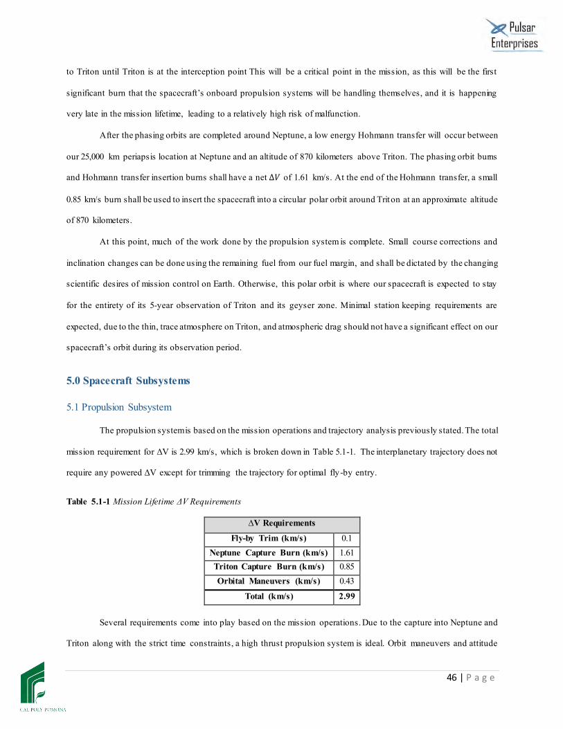
46 | P a g e
to Triton until Triton is at the interception point This will be a critical point in the mission, as this will be the first
significant burn that the spacecraft’s onboard propulsion systems will be handling themselves, and it is happening
very late in the mission lifetime, leading to a relatively high risk of malfunction.
After the phasing orbits are completed around Neptune, a low energy Hohmann transfer will occur between
our 25,000 km periapsis location at Neptune and an altitude of 870 kilometers above Triton. The phasing orbit burns
and Hohmann transfer insertion burns shall have a net ∆𝑉 of 1.61 km/s. At the end of the Hohmann transfer, a small
0.85 km/s burn shall be used to insert the spacecraft into a circular polar orbit around Triton at an approximate altitude
of 870 kilometers.
At this point, much of the work done by the propulsion system is complete. Small course corrections and
inclination changes can be done using the remaining fuel from our fuel margin, and shall be dictated by the changing
scientific desires of mission control on Earth. Otherwise, this polar orbit is where our spacecraft is expected to stay
for the entirety of its 5-year observation of Triton and its geyser zone. Minimal station keeping requirements are
expected, due to the thin, trace atmosphere on Triton, and atmospheric drag should not have a significant effect on our
spacecraft’s orbit during its observation period.
5.0 Spacecraft Subsystems
5.1 Propulsion Subsystem
The propulsion system is based on the mission operations and trajectory analysis previously stated. The total
mission requirement for ΔV is 2.99 km/s, which is broken down in Table 5.1-1. The interplanetary trajectory does not
require any powered ΔV except for trimming the trajectory for optimal fly -by entry.
Table 5.1-1 Mission Lifetime ΔV Requirements
∆V Requirements
Fly-by Trim (km/s) 0.1 Neptune Capture Burn (km/s) 1.61 Triton Capture Burn (km/s) 0.85 Orbital Maneuvers (km/s) 0.43
Total (km/s) 2.99
Several requirements come into play based on the mission operations. Due to the capture into Neptune and
Triton along with the strict time constraints, a high thrust propulsion system is ideal. Orbit maneuvers and attitude

47 | P a g e
control don’t necessarily need a high thrust, but instead low impulse bits and sufficient pointing accuracy. To choose
the best propulsion system candidates, a trade study was made shown below in Table 5.1-2. The performance
characteristics highlighted in red are the most significant design factors towards deciding the ideal syst em for main
propulsion and attitude control.
Table 5.1-2 Propulsion System Trade Study [30]
The high thrust requirements immediately expelled cold gas and electric because it would take too long to
capture into both Neptune and Triton. Solid propellants were expelled because of its inability to throttle, which is vital
to prevent over or undershooting the capture burns. Lastly, monopropellants were expelled because of its low specific
impulse, which could lead to shorter than necessary burns during capture. This leaves bipropellants as the most ideal
for the main propulsion system.
Bipropellant systems utilize either cryogenic or storable propellants. Due to the long mission time, cryogenic
propellants would require too much weight for insulation and too much power for a cooling system. The chosen
storable propellants are hydrazine and variants of nitrogen tetroxide. Hydrazine is chosen because it is the best
performing storable propellant due to its hypergolic properties, specific impulse, and density impulse.[37][38] Thrusters
were researched before concluding on the propellant types because thrusters require different propellants. In Table
5.1-3, a main bipropellant thruster trade study was done to determine not only what thruster would best fit our mission,
but also what propellants are necessary for that thruster. The most significant design factors for this trade study are,
again, highlighted in red.
Cold Gas Monopropellant Bipropellant Solid ElectricTypical Application Attitude Control Orbit/Attitude Control Trajectory/Orbit Trajectory/Orbit Trajectory/OrbitTotal Impulse (N-s) <2,500 <45,000 >45,000 >45,000 >1,000,000Specific Impulse (s) 50-120 180-245 200-468 300 200-8,000
Min Impulse Bit (N-s) 0.0005 0.005 0.025 N/A 0.000001-2Thrust Level (N) 0.01-1 0.2-4,500 25-8,000,000 50,000-20,000,000 0.013
Feed System high pressure gas supply high pressure liquid supply
turbo pump (large) pressure feed (small) N/A high pressure gas
supplyPropellant Type N2,Ar,Kr,H2,He Hyrdrazine w/Catalyst NTO/N2H4 Al,Cl,OH,O2,O3 Ar,Xe,H2,N2,Bi
# of Restarts several thousand several thousand to hundreds of thousand 1 to 4 0 hundreds of thousand
Total Firing Duration several hours seconds to minutes seconds to few minutes seconds to few minutes hours to yearsShortest Firing Duration (s) <0.5 <0.5 <5 N/A <2
Life in Space 10+ years 10+ years 10+ years 10+ years 15+ years

48 | P a g e
Table 5.1-3 Main Propulsion Thruster Trade Study[39][40][41]
Based on the design factors shown, the best balance between thrust, specific impulse and mission experience,
the Aerojet AMBR thruster was chosen. The propellant it uses is hydrazine for fuel and mixed oxides of nitrogen
(MON-3) for oxidizer. The thruster dimensions are with a diameter of 0.362 meters and a length of 0.663 meters. The
nozzle has an expansion ratio of 400:1. One significant property of this thruster is the dual-mode capability.
A very important aspect of hydrazine is that it is capable of being used in a dual-mode system, which is for
both the main propulsion and the attitude control. Utilizing a dual-mode system saves weight and cost of producing
compared to two separate systems. Just as the Juno and Mars Global Surveyor missions featured dual-mode propellant
systems, so will our spacecraft.[42][43] Since a dual-mode propellant system combines the main propulsive thrusters
with the attitude control thrusters, the attitude control propulsive system will be featured in this section. The non -
propulsive attitude control will be featured in its own section.
Now that the thrusters have been chosen, the quantity of propellant can be calculated. This was based on the
∆v requirements stated earlier as well as a desaturation burns for the reaction wheels throughout the mission. The
desaturation burns allocate 20.5 kg of fuel and the rest of the attitude control burns allocate 64 kg of fuel. A fuel
contingency of 5.5% the initial fuel mass was allocated for any potential risks occurring during transit. Using the
rocket equation shown in Brown[31], the total propellant required including contingency for main burns is 1826 kg.
The Aerojet AMBR thruster requires a fuel-to-air ratio of 1.0. Adding the fuel for the attitude control system, the total
fuel mass is 940 kg and the total oxidizer mass is 802 kg.
For propellant tank sizing and material selection, the main factor that came into play was the mass. Several
material types were researched including space-grade aluminum, titanium, and carbon fiber composite. Carbon fiber
composite was the most ideal because it provided the highest strength-to-density ratio. The tensile strength of the
Engine Manufacturer Fuel OxidizerMass(kg)
Power(W)
Thrust(N)
Isp(s)
It(kN-s)
It-min(N-s) O/F
Pc(Bar)
Flow Rate(kg/s)
Experience(# of
Missions)HiPAT Aerojet MMH NTO 5.44 46 445 323 20016 35.6 1 9.4 0.141 100R-4D Aerojet MMH NTO 4.31 46 490 315.5 20016 15.6 1 7.45 0.158 850
AMBR Aerojet Hydrazine MON-3 5.4 45 623 333 5586 1 13.8 0.204 650
TR-308 Dual Mode NGC Hyrdrazine NTO 4.76 46 472 322 11418 - 1 14.13 0.149 N/A
Leros 1b MOOG Hydrazine MON 4.5 46 635 317 13018 - 0.85 16.2 0.204 70
Leros 1c MOOG Hydrazine MON 4.3 46 458 324 14198 - 0.85 16.5 0.144 70

49 | P a g e
composite is 2450 MPa and the density is 1770 kg/m3. Though the manufacturing composite tanks is more complex,
it is one-third of the mass of titanium 6Al-4V tanks.
The composite tank design focused on manufacturing for the best performance. It is important to mention
that since there is more fuel than oxidizer and the density of fuel is lower than the oxidizer, the tank volume for the
fuel tank is going to be larger. It was decided that, to save space and lessen the manufacturing complexity, the fuel
would be split into 2 tanks. Gathered from strength tests and composite behavior analysis, the optimum winding angle
for which to lay the fibers was 54.7 degrees.[44] Per industry standards, a factor of safety of 2.0 was implemented
during these tank design calculations. Assuming a 60% fiber volume, the wall thickness of the fuel tanks are 2.05 mm,
the oxidizer tank is 2.23 mm, and the pressurant tank is 12.75 mm. This converts to 5 fiber layers in the fuel and
oxidizer tanks and 29 fiber layers in the pressurant tank assuming a 0.7 mm thickness per layer. The masses of each
tank including the hardware can be seen in Table 5.1-4.
Table 5.1-4 Propulsion Tank Sizing
As mentioned before, the chosen feed system is a dual-mode system to save weight and cost, and allow the
thrusters to utilize the same system. The system was based on the Mars Global Surveyor propulsion feed system, but
components are altered to lower the weight and complexity. [43] Figure 5.1-1 portrays the feed system with descriptions
of each component.
Tank Type Mass Per Volume Wall Thickness Tank Radius(kg) (m^3) (mm) (m)
Fuel 10.7 0.478 2.05 0.487Oxidizer 13.9 0.616 2.23 0.530
Pressurant 36.5 0.16 13.8 0.352

50 | P a g e
Figure 5.1-1 Spacecraft Propellant Feed System
Each component was researched to keep the mass and power requirements low without losing out o n
reliability. Table 5.1-5 shows a breakdown of the feed system and propellant tanks ultimately providing the entire
propulsion subsystem estimation.

51 | P a g e
Table 5.1-5 Propulsion System Component Breakdown [45][46]
5.2 Attitude Determination and Control System
The requirements for the attitude control system are 0.1 degree pointing accuracy at Earth, a 0.001 degrees
pointing accuracy at Triton, a maximum response time of 100 seconds to rotate the spacecraft about each axis 180
degrees, and maintain stability throughout the mission. These requirements were derived from data trends that were
presented in Brown [3] and from scientific payload requirements. Based on the pointing accuracy requirements, the
only viable method of attitude control is 3-axis stabilized because it provides a high enough pointing accuracy.
The 3-axis stabilization and pointing accuracy will be achieved using a series of different attitude control
sensors. These sensors will determine the orientation of the spacecraft at any given time with respect to multiple stars
and Triton’s orbit. The types of sensors to be used include inertial measurement units, sun sensors, and star trackers.
The IMUs are units that each use 3-4 magnetometers and gyroscopes in order to measure and report the
spacecraft’s angular rate, specific force, and magnetic field. A trade study of IMUs can be seen in Table 5.2-1 with
the major design factors highlighted in red.
Item Listing Quantity Mass (Kg)
Power (W) Supplier
Total Mass (Kg)
Total Power
(W)Fill and Drain Valve 2 0.113 0 VACCO 0.23 0
Fuel Tank 2 10.74 0 NASA 21.5 0Oxidizer Tank 1 13.86 0 NASA 13.9 0
Pressurant Tank 1 36.54 0 NASA 36.5 0Mounting Hardware 1 56.51 0 NASA 56.5 0Pressure Transducer 6 0.113 1 GP:50 0.68 6Temperature Sensor 6 0.226 1 GP:50 1.36 3
Open Pyro Valve 8 0.154 1 VACCO 1.23 0Closed Pyro Valve 7 0.154 1 VACCO 1.08 0
Solenoid Valve 24 0.085 9.8 VACCO 2.04 19.6Latching Valve (No Relief) 3 0.34 1 VACCO 1.02 3
Pressure Regulator w/Filter 2 1.04 0 VACCO 2.08 0Check Valve 8 0.136 0 VACCO 1.09 0Relief Valve 5 0.34 0 VACCO 1.70 0
Flow Balance Orifice 4 0.114 0 VACO 0.46 0System Filter 5 0.114 0 VACO 0.57 0Main Thruster 1 5.4 45 MOOG 5.40 45
Piping 1 12.68 0 NASA 12.7 0Total Mass (Kg) 160.0Total Power (W) 76.6

52 | P a g e
Table 5.2-1 Inertial Measurement Unit Trade Study.[47][48][49]
Based on the following design factors, the CIRUS by Space & Navigation was chosen due to lower power
requirements and higher resistance to white noise error. The CIRUS does have a larger mass, but the lower power
consumption more than compensated for its disadvantages.
The STRs will measure the position of the stars to further achieve a high degree of accuracy for the
spacecraft’s orientation. An STR trade study can be seen in Table 5.2-2, where the major design factors include field
of view, number of stars each can track simultaneously, frequency errors, and lifetime in years. Based on this data,
the AA-STR by Leonardo will be used for its superior field of view and trackable stars compared to the other low-
mass and low-power options.
SIRUTM SIRUTM-L SIRUTM-E MIMU CIRUSManufacturer NGC NGC NGC Honeywell Space & NavigationMass (kg) 7.1 7.1 7.1 4.7 13.5Power (W) 43 43 43 32 25Volume (mm3) 180x149x289 180x149x289 180x149x289 233 (diameter)x169 396 (diameter)x203Bias Stability (deg/hr) 0.0015 0.0015 0.0005 0.005 0.0005Scale Factor Short Term Stability (ppm) <5 10 <5 ≤1 <2Scale Factor Non-Linearity (ppm) <20 <40 <20 - 20High Accuracy Mode Rate Range (deg/sec) ± 7 ± 7 ± 3 - ± 3Noise Equivalent Angle (arcsec) <3 <3 <1 - -Angle White Noise (arcsec/√hr) 0.003 0.009 0.0015 - 0.000025Angle Random Walk (deg/√hr) 0.00015 0.0002 0.00005 - 0.00025Operational Temp Limits (°C) -10 to 60 -10 to 60 -10 to 60 -30 to 65 -20 to 60

53 | P a g e
Table 5.2-2 Star Tracker Trade Study.[50][51][52]
The sun sensors placed on the spacecraft will essentially be a specialized star tracker that exclusively analyzes
the spacecraft's position relative to the sun. These sensors shall be used for gyro updating for the other star trackers,
as well as a failsafe to be used in case of star tracker malfunction. A trade study of three sun sensor candidates can be
seen in Table 5.2-3 with major design drivers highlighted in red. Based on the amount of information found for the
Fine Sun Sensor (FSS) manufactured by Bradford that will be the sun sensor of choice for this spacecraft.
Table 5.2-3 Sun Sensor Trade Study.[53][54][55]
OG-STR A-STR AA-STR SED26Manufacturer Officine Galileo Leonardo Leonardo SodernMass (kg) 2.85 3.55 2.6 3.7Power (W) 8.5-10.5 8.9-13.5 5.6-12.6 9.9-13.5Volume (mm3) 158x146x355 195x175x290.5 164x156x348 170x160x350Dynamic Range (Mi) 1.5-5.5 1.5-5.5 1.5-5.5 -Field of View (deg) 16.4x16.4 16.4x16.4 20x20 -Trackable Stars 10 10 15 10Tracking Rate (deg/sec) 1 2 2 -Acquisition Time (sec) <10 <6 <9 <3Bias Accuracy (arcsec) 13 (all axes) 8.25 (pitch), 11.1 (roll) 8.25 (pitch), 11.1 (roll) 11 (all axes)Low Frequency Error (arcsec) 7 (pitch) 3.6 (pitch) 3.3 (pitch) 4 (pitch)
30 (roll) 21 (roll) 15.6 (roll) 20 (roll)Random Error (at 0.5 deg/sec; arcsec) 15 (pitch) 6 (pitch) 6 (pitch) -
135 (roll) 63 (roll) 49.4 (roll) -Update Rate (Hz) 10 10, 4 10, 8, 5, 4 10Operational Temp Limits (°C) -25 to 60 -30 to 60 -30 to 60 -30 to 60Storage Temp Limits (°C) - -35 to 70 -35 to 65 -40 to 70Lifetime (yrs) 12 18 18 15-18
Coarse Sun Sensor (CSS) Fine Sun Sensor (FSS) Digital Sun Sensor (DSS)Manufacturer Moog Bradford NewSpace Systems Mass (kg) 0.215 0.375 0.035Power Consumption (W) Negligible 0.25 .0375 to .375Volume (mm3) 110 x 110 x 30 108 x 108 x 52.5 34 x 32 x 20FOV (deg) 102 138 140Resolution (deg) - 0.03 -Noise Equivalent Angle (deg) Negligible 0.05 -Alignment Accuracy (deg) 0.16 0.05 0.1Temperature Limits (°C) -80 to 120 -50 to 85 -25 to 75

54 | P a g e
Since the spacecraft will also be utilizing a dual-mode system, the thrusters must use the same fuel type,
hydrazine. Using Table 5.1-2 in the propulsion section, the most ideal type of propulsion system for the attitude control
system is monopropellant due to the high number of pulses as well as the large range of thrust. Using Table 5.2-4
shown below, the ideal thruster was chosen based on the most significant design factors highlighted in red.
Table 5.2-4 Attitude Control Thruster Trade Study[56][57][58][59]
Based on power consumption, thrust level, minimum total impulse and number of pulses, the MR-111C was
chosen as the main attitude control propulsive system. Though the power consumption was not the lowest, it provided
a sufficient thrust level and number of pulses. 12 of these thrusters are located around the spacecraft to provide full 3-
dimensional rotation. Figure 5.2.1 portrays the locations of the attitude thrusters on the spacecraft with their respective
torque arms.
Figure 5.2-1 Attitude Control Thruster Locations
The response time and pointing accuracy for each axis is based on the moment of inertia of each spacecraft
configuration and is presented in Table 5.2-5 below. There are two spacecraft configurations for this mission; the first
Engine Manufacturer Fuel CatalystMass(kg)
Power(W)
Thrust(N)
Isp(s)
It(kN-s)
It-min(N-s) # of Pulses
Pc(Bar)
Flow Rate(kg/s)
(kg) (W) (N) (s) (kN-s) (N-s) () (Bar) (kg/s)MR-103M Aerojet Hydrazine S405 0.16 10.9 0.99 221 122 6.70E-06 515,344 5.9-20.7 0.00045MRM-103D Aerojet Hydrazine S405 1.27 8.25 1.02 224 128 0.03 210,238 5.9-23.4 0.00045MRM-106D Aerojet Hydrazine LCH-207/202 2.7 20.1 40 234 91 0.63 7629 17.2/11.0 0.0174MR-106L Aerojet Hydrazine S405/LCH-202 0.590 41.7 34 229 561 0.15 120,511 4.1-13.4 0.0151MR-111C Aerojet Hydrazine S405 0.33 13.64 5.3 215 260 0.08 420,000 3.4-12.1 0.0025MRE-5.0 NGC Hydrazine N/A 1.5 30 36 232 - - 28,512 4.83-32.75 0.0158MER-1.0 NGC Hydrazine N/A 0.5 15 5 218 - - 457,849 0.55-38.96 0.0023Monarc-5 MOOG Hydrazine N/A 0.49 18 N/A 226.1 614 0.003 205,000 5.5-29.0 N/AMonarc-22-6 MOOG Hydrazine N/A 0.72 30 N/A 229.5 534 0.312 230,000 4.8-27.6 N/A
2.00
m
3.50 m

55 | P a g e
is the spacecraft with the lander attached, and the second is the spacecraft after the lander has detached. For mo st of
the mission life, the configuration will be the first configuration until an ideal landing location is found.
Table 5.2-5 Attitude Control Propulsive System Characteristics
The propulsive attitude control requires propellant to function, but due to the mission consisting of orbiting
a body with disturbances and strict mass limitations, non-propulsive attitude control methods were implemented.
There are several types of non-propulsive control systems available today, all having their advantages and
disadvantages. Table 5.2-6 shows a brief trade study on the three most common types with the most significant design
factors highlighted in red.
Table 5.2-6 Non-Propulsive Attitude Control Trade Study[31]
The most appealing type of non-propulsive attitude control seems to be the magnetic torque rods because it
provides the same torque capability as the reaction wheels at a fraction of the power consumption, but there are some
issues with torque rods that lead to choosing the reaction wheels instead. Triton’s magnetic field is unknown because
the only data we have on it came from the Voyager mission [60]; Neptune’s magnetic field is known to be chaotic and
is very likely to affect any use of torque rods around Triton [61]; and torque rods tend to have a delayed response because
it takes time for the rods to react to the magnetic field. Because the torque rods are low mass and low power, we will
be adding two for experimental control and leaving the main control to the reaction wheels.
Deciding what reaction wheels would most benefit our system came down to the significant design factors
shown in Table 5.2-7 highlighted in red. Reaction wheels tend to fail or malfunction, therefore reliability is one of the
most important to consider. Another method to prevent failure is to include a backup wheel mounted on a gimbal to
Axis of Rotation XX YY ZZ XX YY ZZMoment of Interia (kg-m²) 66934 23453 45865 56682 21535 37379
Input Turn Angle (deg) 180 180 180 180 180 180Pointing Accuracy (deg) 1.43E-05 4.08E-05 1.19E-05 1.69E-05 4.44E-05 1.46E-05
Response Time (s) 92.2 54.6 101.0 84.9 52.3 91.2
Configuration without LanderConfiguration with Lander
Reaction Wheels Control Moment Gyros Magnetic Torque RodsComplexity Medium High MediumReliability Medium Medium High
Mass Medium Medium LowAvg. Power Consumption High Medium Low
Torque Capability 0.001-10 0.1-100 0.001-1Consistency High High MediumDesaturation Yes Yes No

56 | P a g e
replace any of the original three wheels if any were to fail. Momentum capacity is directly proportional to the saturation
time of the wheels due to orbital disturbances, so wheels with high momentum capacity is preferred so that the ACS
thrusters don’t have to desaturate constantly. Reaction wheels also typically consume a lot of power, so the trade -off
between power consumption and momentum capacity was chosen carefully.
Table 5.2-7 Reaction Wheel Trade Study[62][61][62][63]
The Blue Canyon RW8 was chosen because the power consumption remained too high until the momentum
capacity reached around 10 N-m-s and the spacecraft’s power is on a strict budget. The trade-off between momentum
capacity and power consumption was close where the momentum capacity of the Honeywell HR16 provided a
saturation time 9.4 times the saturation time of the Blue Canyon RW8, but the power consumption was 10.7 times the
consumption of the RW8. It was decided that the power consumption was more important because the power budget
is too strict. The RW8 mission life isn’t ideal, but the implementation of another reaction is expected to extend the
overall life of the non-propulsive attitude control system. The reaction wheels were also tested to determine the
pointing accuracy and response time to turn the spacecraft about each axis by 90 degrees. Table 5.2-8 portrays those
response times for each spacecraft configuration. The response times are unreasonably high, but if any quick axis turns
are necessary, then the attitude control thrusters must take over.
Table 5.2-8 Reaction Wheel Pointing Accuracy & Response Time
As for the experimental torque rods, we looked for one that would require low power consumption of the
reaction wheels so that our experimentations don’t put us over the already strict power budget fairly and a large torque
Name ManufacturerMass(kg)
Peak Power(W)
Steady Power(W)
Wheel Speed(rpm)
Momentum(Nms)
Torque(Nm)
Life(years)
Vibration(Grms)
HR12 Honeywell 7 105-195 22 6000 25 0.1-0.2 15+ 13.8HR14 Honeywell 8.5 105-195 22 6000 50 0.1-0.2 15+ 13.8HR16 Honeywell 10.4 105-195 22 6000 75 0.1-0.2 15+ 13.8HR0610 Honeywell 4 80 15 6000 8 0.055 10+ 19.8RWA-15 L3 14 230 17 2200 20 0.68 7+ -RW8 Blue Canyon 3.6 80 7 6000 8 0.11 10+ -RSI 12-75/60 Rockwell Collins 4.85 90 20 6000 12 0.075 15+ -RSI 68-170/60 Rockwell Collins 9.5 150 20 6000 68 0.17 15+ -
Axis of Rotation XX YY ZZ XX YY ZZMoment of Interia (kg-m²) 66934 23453 45865 56682 21535 37379
Input Turn Angle (deg) 90 90 90 90 90 90Pointing Accuracy (deg) 2.12E-08 6.05E-08 3.09E-08 2.50E-08 6.58E-08 3.79E-08
Response Time (s) 978 579 809 900 555 731
Configuration with Lander Configuration without Lander

57 | P a g e
output to prevent any delayed response that would cause an excessively slow response time. This leads to creating a
trade study shown in Table 5.2-9 where the significant design factors are torque and power
Table 5.2-9 Magnetic Torque Rod Trade Study[66]
The torque rods chosen are the MTB300-L-28V because they are half the power consumption and double the
torque output of the reaction wheels chosen. The spacecraft will mainly be in a polar orbit so the torque rods will be
oriented into Triton’s core and perpendicular to its orbit so that it can conduct longitudinal changes and in -plane twist
maneuvers.
The final component list of the attitude determination and controls are shown below in Table 5.2-10. The
total power represents all the components being on at the same time, but the torque rods would turn on once the
reaction wheels turn off for experimentation.
Table 5.2-10 Attitude Determination & Control Component List
5.3 Command and Data Handling
A significant bottleneck in our data acquisition mission is our telecom system. While our instruments are
more than capable of taking massive quantities of data, due to the distance between Earth and our spacecraft, and the
possible size of our spacecraft, the transmission rate of such data is going to be severely limited.
MTB NameDipole Moment
Guaranteed (Am²) Torque (N-m)
Current (mA)
Mass (kg)
Power (W)
Length (m)
MTB200-L-28V 213 0.158 184 4.06 2.74 1.07MTB240-L-28V 231 0.172 190 5.00 3.34 1.13MTB300-L-28V 273 0.203 184 5.62 3.48 1.25MTB450-L-28V 450 0.335 236 8.93 3.95 1.39MTB550-L-28V 524 0.390 228 9.79 4.06 1.53MTB650-L-28V 683 0.509 356 12.3 5.36 1.46MTB750-L-28V 692 0.515 281 13.2 5.21 1.63
Item Listing Quantity Mass (Kg)
Power (W) Supplier Total Line Mass
(Kg)Total Line Power
(W)ACS Thrusters 12 0.33 13.64 Aerojet 3.96 27.28Reaction Wheel 4 8.5 7 Blue Canyon 34 28
Magnetic Torque Rod 2 5.6 4.0 Cayuga Astronautics 11.2 7.91Gyroscopic Controls 1 13.5 25 Space & Navigation 13.5 25
Star Trackers 3 6.47 9.9 Sodern 19.41 19.8Sun Trackers 1 0.375 0.25 Braford 0.375 0.25
Total Mass (Kg) 82.49Total Power (W) 108.24Power (Prop Mode) (W) 72.33Power (Non-Prop Mode) (W) 73.05

58 | P a g e
Our mission architecture requires two antennas, for high gain and low gain transmission and receiving.
Received commands will be pre-processed on an uplink card, and telemetry to be transmitted will be formatted by a
downlink formatter, which will use a Reed-Solomon (255,223) encoding to increase reliability in the transmitted
signal. These commands and telemetry will be processed by our radiation hardened on board processor, the 12 MHz
Mongoose V.
Figure 5.3-1 Data Processing Flow
Due to the vast difference in transmission distance, the low gain communication links between the lander
and the orbiter will have much higher performance than the high gain link between the orbiter and the Earth.
However, this data will need to be buffered on the orbiter before it can be transmitted to the DSN. This will increase
the data storage requirements of the orbiter, which will have two 12 TB solid state recorders.
While all our instrumentation will contribute to the overall data storage requirements of the orbiter, the
clear majority of raw data that will be collected by the orbiter will be from its visible imagine cameras, which will
be performing a full mapping of Triton’s surface as Triton revolves underneath the orbiter’s polar orbit. This surface
mapping imagery shall be collected by the HRCC, UVS and VIS at a rate of 10.08 megabits per second. Every other
instrument shall be commanded to point at specific targets of interest at specific times, however, the visible camera
shall be pointed towards the surface as often as possible to maximize image collection of the surface. With
continuous coverage, it will take two months to collect a complete image of the surface. However, to limit the
amount of data that must be stored, significant pre-processing must take place to shrink the size of the data collected.
Many portions of the surface will be passed over multiple times due to the inters ection of subsequent orbits. These
sections shall be checked for image quality and then cut and spliced together to form on continuous image of the

59 | P a g e
moon’s surface. This will shrink the volume of imagery that must be transmitted to the DSN. Furthermore, our data
volume shall go through a lossless compression algorithm to shrink its size even more. With the similarity in color
pallets of the features on Triton, and the signal noise found in images from New Horizons, we’re expecting a
compression ratio of at least 60%. Table 5.3-1 displays the component breakdown of this subsystem.
An important aspect of the command and data handling system is the fault protection. Fault protection
implements software coding to detect, assess, and mitigate subsystem faults such as a valve malfunctioning. An
estimated three million lines of code have been incorporated into the subsystem and an additional two million lines
of code was incorporated solely for fault protection.
Table 5.3-1 Command and Data Handling Component Breakdown
5.4 Telecommunications
The requirement for the telecommunications system on the orbiter states that all data necessary to fulfill the
RFP requirements must be done so by the end of the mission in December of 2040. This allows five full years to
transmit instrument data from the orbit of Triton to earth’s DSN. The orbiter will be allowed to transmit data to the
DSN for 8 hours per Earth day, for the entire duration of the mission. The orbiter will implore the use of the X-band
frequency and with transmit data at a frequency of 8.42 GHz using a 3.0-meter parabolic HGA shown in Figure 5.4-
1. The largest challenge for the transmission of data is the enormous distance between Triton and Earth.
Figure 5.4-1 3.0-meter Parabolic HGA

60 | P a g e
With 50 W of power and the spacecraft located 4.7 billion km from Earth, the antenna will have a maximu m
and minimum downlink rate to the DSN of 13 kbps and 6.5 kbps, respectively. Using Reed-Solomon turbo coding the
spacecraft’s telecommunications system will have the capability to transmit 15/7.5 ksps. Over the five years the
spacecraft will orbit Triton, this translates to a maximum of 683 Gbits and a minimum of 341 Gbits of science data
that can be transmitted from the spacecraft to the DSN. Due to the vast distance the signal must travel, the ACS system
must be able to keep a pointing accuracy of 0.10 degrees to maintain constant contact with the DSN. The HGA will
be mounted to the spacecraft bus opposite from the spacecraft payload so that the payload can take data while the
HGA transmits are specified location in orbit. A low gain antenna is also placed atop the HGA, however, will only be
used for close communication with at beginning of the mission and if there is a need for emergency uplink at any
point.
To communicate with the Triton lander, an Electra UHF radio (shown in Figure 5.4-2) will be included to
the telecommunications system of the orbiter, as well as an Electra-Lite UHF radio on the lander.[67] These radios
allow for high data transfer rates at minimal power consumption between the spacecraft and the lander. The Electra
requires 67W to transmit and 30W to receive, however due to the nature of the landers objective, the Electra on the
orbiter will almost exclusively be receiving. Due to its power consumption, main communications to the DSN will be
halted for 1.51 hours while the lander transmits all of its data to the orbiter as it passes over. A helical antenna (Figure
5.4-3) on the lander will be used to transmit from the Electra-Lite at 390-450 MHz to its parent radio on the orbiter.
The helical antenna provides a 180-degree field of view. Using 40W, the Electra-lite can transmit between 2
and 2048 kbps to the orbiter. During the 1.51 hour fly over of the orbiter, the lander will transmit between 8.2 M bits
and 8.4 Gbits of data back to the orbiting vehicle. The orbiter will act as a relay and transmit the data obtained by the
Figure 5.4-2 Electra UHF Radio Figure 5.4-3 Helical UHF Antenna

61 | P a g e
lander instrument to the DSN. This will allow for all RFP required data to be transmitted to earth before December of
2040. Table 5.4-1 shows the breakdown of the mass and power for the telecommunications subsystem.
Table 5.4-1 Mass and Power Statement for TES Telecommunications Subsystem[68][69]
Equipment Mass (kg) Power (W)
Electra Radio & UHF Antenna 7 10
Telecom Panel 20 0
Antenna (High Gain, Low Gain) 30 0
SDST 10 2
SSPA (x2) 3 50
Total 70 62
Total (Xmit to DSN) 52
Total (Rx from Lander) 37
5.5 Power Subsystem
The power subsystem is the heart of the spacecraft, essentially keeping all other systems alive and runn ing
during the course of the mission. This is an integral part of the system, therefore, the choice of power supply was
critical in the design process. Primary batteries, while effective, would be too heavy and unpractically large for a
mission length of over 18 years. Fuel cells were also explored as an option, however the size and weight associated
with the system and tanks for the fuel were also too large under preliminary estimates to be a viable option. Solar cells
are generally the best option for spacecraft power, but only within a certain distance from the Sun. As we get further
from the Sun, the solar flux received by it decreases drastically, and in order to receive enough power at Triton from
solar cells, the solar array would be approximately 1.46 × 10⁸ square meters. This size is ridiculously large and heavy,
therefore solar cells are not a feasible option. Nuclear reactors were also considered as an option, but no practically
tested nuclear power sources have been created for satellites. The combination of R&D and lack of support from the
public would make this a poor choice of power supply for the mission. The only final option we had for our power
supply was using radioisotope thermoelectric generators (RTGs).

62 | P a g e
RTGs have been in use by satellites since the beginning of human exploration; Apollo 12 on the moon in
1969, Voyager 1’s deep space mission in 1977, and even the Curiosity Rover on Mars’ surface in 2011 all utilized
RTGs. In total, the US has had 26 mission using 45 RTGs total and they have never been the cause of an accident.
This makes the RTGs a very reliable source of power. RTGs have been used for very similar missions, have a
reasonable mass-to-power output, a high reliability, and are perfect for long missions in deep space. There are many
types of RTGs that could be used for this mission. One option is the use of General Purpose Heat Source (GPHS)
RTGs, which have very high power outputs. However, these types of RTGs are currently out of production and,
economically speaking, to restart production for a single mission would be unrealistic. Multihundred-Watt (MHW)
RTGs were used on Voyager 1 and 2, but they too are out of production. The next generation of RTGs , known as
Advanced Stirling radioisotope generators (ASRGs) boast a higher system efficiency of 23%, a higher electrical power
output, a smaller size and a mass compared to previous RTGs. They also keep 85% of their power after 14 years.[72]
ASRGs, however, have had many setbacks and will not be ready until 2028. [10] Although this RTG would be ideal,
they are unavailable for Project TES. The last RTG analyzed was the Multi-Mission RTG (MMRTG). Alice Caponiti,
the DoE’s Director of Space and Defense Power Systems, stated that there are two MMRTGs still available for launch
by December 31, 2021, and new RTGs can be produced within 5 years.[70] Given this is an RTG still within pour
timeline, and it gives reasonable efficiencies and power outputs, it was chosen for Project TES. An example of an
MMRTG can be seen in Figure 5.5-1 below.
Figure 5.5-1 MMRTG with Various Components [71]
From the power budget in Section 3.2 and lifetime assessment in Section 10.0, which will be discussed later,
four MMRTGs were chosen to act as the spacecraft’s primary power source. Per NASA, each MMRTG contains 3.52
kilograms of Pu-238, the main power source, which provides 2,000 W of thermal power and 110 W of electrical power

63 | P a g e
at beginning of life. Each unit has a mass of 43.6 kg.[71] As mentioned before, 2 MMRTGs are currently available for
future missions, both of which Project TES will utilize. The other two MMRTGs must be manufactured. In a Report
to Congress given in June 2010 titled Start-Up Plan for Pu-238 production for Radioisotope Power Systems, 1.5
kilograms of Pu-238 would be produced and allocated each year for scientific purposes. Given each RTG requires
3.52 kilograms and 5 years to manufacture, the other two will be available by the launch date of 2022.
RTGs are the main power supply, however there is a multitude of support systems that are associated with
the main power subsystem. These support units are generalized into three main categories Power Distribution Units
(PDUs), Power Regulatory Units (PRUs), and cabling. New Horizons’ spacecraft block diagram can be seen as an
example in Figure 5.5-2 which will be used as a model to design TES’s satellite power subsystem. A fully redundant
PDU complete with temperature sensors will be utilized within the power subsystem which will be able to distribute
power to the various other systems within the spacecraft. External thermal shunts and a shunt PDU will also be
implemented to control excess power from the RTG. The shunt PDU will control the amount of power needed to be
rejected in the form of heat or the amount of power to recover by the rejected heat depending on the specific mode the
spacecraft will be in. The wiring will be used to connect the various electrical components to the PDU and MMRTG
unit. Project TES’s power block diagram can be seen in Figure 5.5-3.

64 | P a g e
Figure 5.5-2 Reference New Horizons Spacecraft Block Diagram [73]
Figure 5.5-3 Project TES’s Satellite Power Block Diagram

65 | P a g e
The compilation of the various spacecraft power subsystems can be seen within Table 5.6-1. There will be
no batteries within the spacecraft because the MMRTGs power output is consistent and reliable enough that simple
capacitors can be used as redundancy in the PDU. The PDU, PRU, mounting hardware, and cabling are estimated
values using Brown’s past mission estimation correlations.[3] Estimations are used to accurately determine the mass
and power since previously used equipment can not necessarily be applied to this specific mission and therefore much
be made custom to the spacecraft needs.
Table 5.5-1 Power Subsystem Mass and Power Statement
5.6 Thermal Control Subsystem
Thermal control of the spacecraft is difficult to analyze because there are many variables that effect the
temperature of an object. In space, there are only two forms of heat transfer: radiation and conduction. Conduction
occurs within two materials that are close enough to one another that they are physically ‘touching’ and a transfer of
energy occurs which either raises or lowers the temperature. This heat flux will only occur on the spacecraft itself for
the individual components, interactions, and subsystems that will be in direct contact with one another. Radiation is
the transfer of energy through waves or particles, this can occur in a vacuum or through a physical medium such as
Earth’s atmosphere. Due to the laws of physics, the only real way for a spacecraft to remove the heat or energy is to
radiate it away from itself. Heat generation can be internal such as the through electronics or Pu -238 within the RTG,
but can also occur with radiation from the Sun or other planets.
The first step in understanding any thermal control situation is understanding the surrounding temperatures
without the added thermal control to accurately size the system to either raise or lower the temperature. Figure 5.5-1
shows the maximum and minimum temperature limits the spacecraft will experience leaving Earth. The power
dissipation includes the amount of electronics that will be power on during this segment which is highly dependent on
the mode the spacecraft will be in. The lower temperature limits show if the spacecraft is in complete shade around
Item Mass (kg) Power (W) Batteries 0.00 0.00
(4) MMRTGs with Attachment Hardware
174.40 0.00
Power Regulatory Unit, Power Distribution unit, Shunts
36.12 45.00
Electrical Cabling 11.21 14.00 Total Power Subsystem 221.72 59.00

66 | P a g e
Earth and the higher temperature limits show if the spacecraft is in direct sunlight, therefore the temperature range the
spacecraft can possibly be in departing from Earth is shown. Figure 5.5-2 shows the temperature limits during transit
when the spacecraft is within its transfer mode. As the distance from the sun increases the temperature of the spacecraft
will decrease which is to be expected. Figure 5.5-3 shows the temperature limits at Triton which are also within the
specified limits however at Triton the sun has less influence of the spacecraft therefore the lower and higher
temperature range is much shorter than at Earth.
Figure 5.6-1 Temperature Limits at Earth
Figure 5.6-2 Temperature Range During Transit

67 | P a g e
Figure 5.6-3 Temperature range at Triton
At Earth, radiators are required to keep the temperature down into the temperature limits of the spacecraft.
During transit and arrival at Neptune, power is required to raise the temperature of the spacecraft to opera ting limits .
Limits of the various spacecraft subsystems are shown in Table 5.5-1 below.
Table 5.6-1 Temperature Limits of Spacecraft Subsystems
Subsystems Lower Limit (°C) Upper Limit (°C) Electronics and Payload Sensors 0 40 Hydrazine Fuel 7 35 Oxygen Oxidizer -11.2 21.2 Infrared Detector Sensors -200 -80 Structures -46 65 RTGs -46 200
There are two types of thermal control systems: active and passive. For this unmanned spacecraft , a passive
thermal system will be utilized because it is lighter, requires less power, and is cheaper.[72] This passive thermal control
will utilize passive copper heat pipes, radiators, louvers, thermal switches, RHUs, and multi-layer insulation. A
schematic of these components are shown in Figure 5.5-4.

68 | P a g e
Figure 5.6-4 Passive Thermal System for Spacecraft
The passive copper heat pipes have a diameter of 1.27 cm and are used to transfer heat away from the RTG
to the various subsystem in the spacecraft. This is ideal because the RTGs will output 8,000W of thermal power a t
BOL and this will be utilized instead of heaters to save weight and cost. The thermal switches are made from
Honeywell and will be implemented at key locations of thermal conduction paths; they will respond to temperature
sensors and will open or close the conduction paths to allow heat flux to flow or become disrupted from the heat pipes.
The multi-layer insulation will be composed of 12 alternative layers of a light weight film known as Kapton with
internal layering of Mylar support material with 5-mil Chromium vapor deposited coating that will provide an
emissivity of 0.24 and absorptivity of 0.57.[74] This will be used to insulate key parts such as the structure and fuel
tanks by allowing less radiation heat to escape from those areas. 16 RHUs will als o be implemented to insure a steady
heat flux to the structure of the spacecraft as well as the key electrical subsystems. Radiators will be used to release
excess heat from the spacecraft using principles of radiation control. These radiators will be pass ively controlled with
louvers which will control rate of heat flux with bimetallic springs that actuate the louvers’ blades on the radiators at
specific temperatures. Below is the mass statement for the passive thermal control system including the power an d
mass calculations per the spacecraft’s needs. To meet the lowest upper limit that the spacecraft can handle the largest
radiator surface area is sized at 62 square meters insuring the spacecraft does not over heat at Earth. Past Earth the
radiators will mostly be inactive and will not be radiating any excess heat. At Triton and during transit, it was found

69 | P a g e
that the RTGs will sustain the spacecraft temperature lower limits through conduction of the heat pipes and thermal
switches and temperature sensors. Table 5.5-2 shows the thermal control component’s mass and power final
calculations.
Table 5.6-2 Thermal Control Components Mass and Power
Component Mass (kg) Power (W) Heat Pipes 9.99 0 2 Radiators 7.88 0
3 Thermal Switches 0.06 1 16 RHUs 0.64 0
Multi-Layers Insulation 1.49 0 3 Temperature Sensors 0.09 0.5
Totals 20.15 1.5
5.7 Structural Elements
The main body of our spacecraft will be a hexagonal structure to incorporate all the payloads to be facing the
target and the placement of the subsystems to be equally distributed. The hexagonal structure is constructed with 7075-
Aluminum that have properties that can withstand the shear and axial loads of all the payload instruments and
subsystem mountings on the spacecraft. An aluminum construction will allow for a higher technical readiness level
as it will be feasible to construct the body frame.
In designing the body frame, the extreme load conditions were taken into consideration. The extreme load
condition of the spacecraft is the launch loads which is found through the SLS Mission Planner Guide shown on Table
5.7-1. From the SLS launch vehicle, the maximum launch load is 3.5g’s. Based on that acceleration, the launch loads
were determined by the mass of the spacecraft multiplied by the acceleration. This force was distributed of the bottom
section of the payload where the payload attach fitting is connected.
Table 5.7-1 Missions Planner Guide Launch Loads [31]

70 | P a g e
In the initial structure analysis, the main body frame showed a high deflection shown o n Figure 5.7-1, where
the propulsion system was mounted. This resulted in a very high risk for the structure for failure in the propulsion
system thus a revised design was created.
Figure 5.7-1 Payload Bus FEA Launch Load Analysis
For the second revision, a beam was used going along the top and bottom part of the structure to add support
to the base. This reduced the deflection from the base and created a well distributed stress along the structure. However,
the beams were prone to buckling. Thus, the final revision placed a plate at the middle of the structure to address the
stability to the columns. The structural analysis of the payload bus is shown below on Figure 5.7-2. The extra holes
on the payload bus were created to reduce the mass of the structure.
Figure 5.7-2 Payload Bus FEA Final Revision Launch Load Analysis

71 | P a g e
6 Lander Overview
6.1 Determination of Landing Site
The second phase to the science mission involves the Vespucci lander. Vespucci shall detach from TES and
soft land on Triton’s surface to conduct surface composition analysis and take high resolution surface photographs.
The TES Orbiter will spend just over a year mapping Triton’s surface to determine an ideal landing site. The most
beneficial landing site was determined to be in the geyser region near the plumes because Vespucci will be able to
retrieve data of Triton’s surface as well as geyser precipitate composition. This data alone would be difficult to
differentiate what is surface material and what is geyser precipitate material, but, in conjunction with TES’s geyser
plume data, the two can be separated and identified. The HRCC and VIS onboard the TES Orbiter will be used to map
Triton’s geyser region to a ground resolution of 7 meters per pixel.
Vespucci will face some obstacles during its descent. Although the HRCC and the VIS provide a detailed
ground resolution, they may not accurately identify smaller geological features that may complicate the landing. This
could cause Vespucci to land on an uneven surface and possibly topple over. Another obstacle is that Triton’s surface
may be softer than expected, which could lead to Vespucci falling through a hollow surface. These obstacles may
delay the landing phase until sufficient data is retrieved by TES.
6.2 Subsystems
One of the crucial part of our missions is the ground science operations. Our mission designed a lander that
will take data and transmit data to the main spacecraft. The lander subsystems will have all the subsystems that the
main spacecraft contain which are the following: Power, Structures, Thermal Control, Propulsion, Attitude Control
System, Command and Data Handling, and Telecommunication.
Unlike the main spacecraft, the lander power system will be utilizing Lithium Ion Cells that will power the
entire vehicle. At peak operations, the landers maximum power output is 100 W. Using the maximum power output
to design the power system, the lander will require 14 cells in series and as redundancy, it will have another line of
that in parallel. The total mass of the Lithium Ion cells in the power system is approximately 30.24 kg using the
Lithium Ion specification shown below in Figure 6.2-1. The entire power system will be a total of 44.41 kg with 7 kg
for the power control electronics and another 7 kg for the cabling weight.

72 | P a g e
Figure 6.2-1 Saft Lithium Ion Cell Specifications[18]
For the thermal control system, a lumped mass analysis was performed. The extreme conditions for the
lifetime of the lander will occur for the extreme hot during take-off, and extreme cold when the spacecraft landed on
Triton. Based on the lumped analysis, the lander will be in sufficient temperatures for the extreme hot condition with
a multilayer insulation. However, at Triton the lander will be below its acceptable operational and nonoperation al
lower limits. Therefore, the lander will require external heaters to keep the temperature of the lander to its acceptable
temperature limits.
For the Command and Data Handling system, the total amount of data the scientific payload will take is at
least 16 GB. The lander will have an onboard storage of 16 GB of data storage. The onboard processing unit will also
take control of the spacecraft and receive all its commands from the main spacecraft and send its status information
to the main spacecraft.
One of the crucial subsystem for the lander is the propulsion subsystem. Descending from 800 km above the
surface of Triton, the propulsion system will be heavily reliant on the descent of the spacecraft. Calculating the descent
velocity of 1150 m/s from 800 km, the total propellant for a safe landing on the surface of Triton is 48 kg. The total

73 | P a g e
subsystem mass which includes the propellant tank, the engine, the valves, and other miscellaneous components will
be 31 kg.
To control the descent of the lander, the attitude control system will be controlling the descent of the
spacecraft. The attitude control system will be using thrusters to control the 3 axis rotations of the lander. The thrusters
on Vespucci are the same as the one used on the TES.
For the structures subsystem, the lander will experience a total energy of 0.1 J of energy during landing. The
amount of energy the lander will be experiencing at landing is negligible, our analysis for the lander’s structure is
based on the propulsive burns during the descent stage of the lander. The propulsion system loads the lander with 440
N of force. Thus, a circular structure made with 7075-Aluminum will be used. Thus, the total subsystem mass of the
structure will be 50 kg. The total dry spacecraft mass is 110.8 kg. The lander mass statement is shown below as Table
6.3-1.
Table 6.2-1 Lander Mass Statement
Subsystem Budget (kg)
Current (kg)
Power 15 29.29 Structures 21 21
Thermal Control 2 2 Propulsion 10 31
Command and Data 5 5 Attitude Control ACS 7 19
Telecom 5 5 Cabling 6 0 Payload 9 9
Budget Total 80.00 120.87 Dry Mass Margin 24.00
On-Orbit Dry 104.00 120.87 Solid Propellant 30.00 63.2
Cold Gas Propellant 8.00 0.45 On-Orbit Wet 142.00 184.50
7 Project Management Plan and Schedule
7.1 Project Management Plan
In conjunction with the JPL Project Haukadalur RFP, the AIAA Space Launch System RFP served as the
basis for our undergraduate senior design project. Similar to industry, the RFP provided set specific requirements and
deadlines for the proposal and design. To meet said requirements and deadlines, a project management plan was
implemented. The plan would incorporate the capabilities of the team and the deadlines for the RFP into a design

74 | P a g e
schedule, which includes conceptual design, preliminary design, and detailed design. Conceptual design focused more
on mission architectures, while preliminary and detailed design focused more on spacecraft design.
To effectively manage the workload of the project, a work breakdown structure was created to define the
elements that were involved in spacecraft design from conceptual design to end of mission life shown below in Figure
7.1-1. Each design subsystem was assigned a lead based on their knowledge and experience prior. A deputy was also
assigned under the lead to provide back-up and review completed work. One team member was given the role of
systems engineer to implement proper measures that would prevent integration, manufacturing, or disposal issues.
Such measures include reviewing the progress of each member during the weekly meetings and identifying any
problems that may occur with other subsystems or further down the design timeline; communicating between
subsystems to make sure future work is on the same page; thoroughly identifying potential project risks and
introducing mitigation measures; and continuously checking back with the RFP to make sure all work is satisfying the
requirements.
Scientific Spacecraft
System0.0
Space Vehicle
1.0
Launch Systems
2.0
Program Management/Systems Engineering
3.0
Telemetry and Data Collection
4.0
Ground Support/Orbit Maintenance
5.0
Propulsion1.1
Payload1.2
Attitude Control System
1.3
Aerodynamics1.4
Communication & Telemetry
1.6
Structures1.7
Power System1.8
Feed System1.1.2
Hardware1.2.1
Thrusters1.3.1
Controls1.3.2
Planetary Data System/Radio
1.6.1
Materials1.7.1
Load Analysis1.7.2
Power Supply1.8.1
Temperature Control
1.9.2
Radiation/Environment
1.9.3
T0.1T0.2T1.1T1.2T0.3T0.4T0.5T1.3T0.6
T1.1T0.6T1.4
T0.7
Integration & Assembly
1.10
Instrumentation1.3.3
Articulation1.2.2
T0.10
T0.8T1.5
T0.9T1.6
T0.11C0.1M0.1M0.2
Thermal Control
1.9
Engines1.1.3
Astrodynamics1.5
Propellant System
1.1.1
Trajectory Analysis
1.5.1
Orbit Determination
1.5.2
Lander Vehicle
1.11
T0.1T0.2T1.1T1.2T0.3T0.4
Figure 7.1-1 Work Breakdown Structure with RFP Requirements Interface
The proposal was broken up into development phases and placed into specific school quarters; conceptual
design in fall quarter, preliminary design in winter quarter, and detailed design in spring quarter. Weekly meetings,
both in class and at least one on the weekend, were chosen so that the team could communicate progress of individual

75 | P a g e
work, present any issues that they had with the team to solve together, and make team decisions on important choices
such as determining what payload items would be most efficient to the mission. Progress reviews were also
incorporated into the weekly meetings to make sure everyone is staying on track with the schedule so that other team
members aren’t waiting on their work or the team isn’t bombarded with catching up as the project report neared.
During winter quarter, the team was given the opportunity to present in front of faculty and industry from
Northrop Grumman and Jet Propulsion Laboratories. The audience consisted of employees in the following fields:
systems, structures, manufacturing, materials, communications and telemetry, and payload. Following the
presentations, the audience graciously provided feedback on the designs. The presentations proved to be invaluable
because it allowed the team to re-evaluate subsystem designs and find alternatives.
7.2 Project Schedule
The program management plan incorporates the conceptual, preliminary, and detailed design. The conceptual
design has multiple reviews including mission concept review, alternative concept review, systems requirements
review, and system design review. The preliminary design only includes the preliminary design review and the detailed
design only includes the critical design review. The conceptual design incorporates more reviews because of the wider
scope it must cover to ultimately down-select to one design, whereas the preliminary and detailed designs only focus
on a single design.
The program reviews are defined by the large red arrows at the top to show how many reviews are in play
during the mission program as well as the white downward facing triangles after each task to show which review is
for which task. As seen in the schedule in Figure 7.2.1, the conceptual and preliminary design sections of the program
are shorter than typically seen in industry because of our senior design course limited these tasks to a mere 3 months
per. As for the remaining program tasks, due to strict trajectory limits, the detailed design was allocated 2 years, and
manufacturing and testing was allocated 2 years.

76 | P a g e

77 | P a g e
8 Assembly, Test, and Launch Operations
The ATLO process shall consist of a series of completing engineering data, manufacturing components and
subsystems, testing components, integrating into a whole spacecraft, and preparing for launch. This process is
projected to last approximately four years, in order to ensure adequate manufacturing and testing of all components
prior to launching. Each step is briefly described in Table 8.1; the process is modeled after the third edition of “Space
Mission Analysis and Design” (Chapter 12, Table 12-3).
Table 8.0-1 Steps of Assembly, Testing, and Launch Operations.[75]
Step Description Length of time Prepare Engineering Data Complete schematics with dimension,
specifications, materials needed, processing methods
1-6 months
Manufacture Components -Manufacturing planning -Procurement and testing
-Assembly -Acceptance testing
1-6 months (parallel with engineering data prep)
-Electronic parts: 3-18 mos. -Assembly: 1-3 mos.
Qualify Components Functional testing and environmental exposure
1-6 months, depending on component and environment
Integrate, Prelaunch Test Spacecraft Mechanical assembly, environment exposure, construction of spacecraft
6-18 months
Engineering data shall consist of schematics which include specifications of component s/subsystems, as well
as procedures on how to manufacture and integrate them. Each component shall have its own schematic, and various
schematics will combine in order to show how they are to be manufactured, tested, and integrated with each other.
Furthermore, the engineering data will show mounting and encapsulation procedures.
The manufacturing processes will involve raw materials from third party vendors, and different clean rooms
shall be utilized to manufacture different categories of components (mechanical, inertial instruments, electronic,
optical, etc.). While the mechanical manufacturing (plating, chemical treatment, composite manufacture adhesive
bonding, etc.) will not require any controlled cleanliness, all other categories will require clean rooms ranging from
Class 100 to 10,000. This stage (along with testing) is where quality assurance will be used to ensure all components
are in compliance with engineering data. All failed pieces and anomalies will be kept in order to document repeated
failures and rectify any design weaknesses.
Testing of components for this mission will include functional tests where components must be able to
withstand adverse vibration, shock, and thermal conditions. Vibrations testing will simulate launch vehicle acous tics

78 | P a g e
and engine rumble by giving random-signal frequencies ranging from 20 to 2,000 Hz. Shock tests will simulate
payload fairing separation and spacecraft separation bolts, while thermal tests shall simulate the conditions the
spacecraft will face. For example, any component that contributes to the lander must be able to function under
temperatures as low as 35 K (-238°C). Functional tests for each subsystem will be conducted, such as static launch
load tests, pattern tests for antennas, and closed-loop tests for attitude control systems.
The components shall be transported to the launch site for final spacecraft assembly. At the launch site, the
spacecraft shall be inspected, propulsion systems tested, propellant loaded, mating spacecraft to the SLS Block 1B,
and monitoring until the vehicle is prepared to launch.
9 Technology Readiness Level
Many of our components had to be addressed for TRL concerns. Subsystems including payload, propulsion,
structure, attitude control, thermal, and power were analyzed to determine how much new technology was being
implemented, and thus, how high the overall risk for our entire spacecraft system was. We used NASA’s outlined
definitions for our criteria in selecting the correct TRL for each component.[29] Almost all items in our subsystems
were deemed to be a 9 on the TRL scale, meaning they were proven, ready to use, and reliable. Only three of our
technologies have a TRL of 7, since they are still developing prototypes. Specifically, these were our composite tanks
for propulsion (carbon fiber), our composite magnetometer boom, and our eMMRTGs. Our TRLs for all our major
components are listed below in Table 9.0-1.
Table 9.0-1 Tech Readiness Levels
Subsystem Technology Technology Readiness Level Payload Science Payloads (collective) 9
Propulsion Composite Tanks 7 Propulsion Thrusters (AMBR) 9 Propulsion Valves 9 Structure Magnetometer Boom 7
ACS Thrusters (MR-111C) 9 ACS RWAs 9 ACS Torque Rods 9 ACS Sun Sensor 9 ACS Star Trackers 9 ACS IMUs 9
Thermal Radiator 9 Thermal Louvers 9 Thermal RHUs 9 Power MMRTG 9 Power eMMRTG 7 Power PDU 9

79 | P a g e
10 Mission Lifetime Assessment
As talked about in previous sections, the mission lifetime is rather long and encompasses almost two decades.
Phase-1 of the mission from Earth to a Saturn flyby will last approximately 2 years and 326 days, Phase 2 from Saturn
to Neptune 10 years and 130 days, Phase 3 from Neptune to Triton arrival 65 days, Phase 4 Triton arrival to end of
operations 4 years and 106 days, and Phase 5 from end of operation to end of data delivery 1 year. In total, the mission
Duration is 18 years and 262 days. Making this one of the longest sustained missions ever tackled by man. With
mission length comes complications in sustainability, survivability, and operational as sessment. The two main lifetime
assessment criteria that were analyzed were the power subsystems as well as the propellant usage by the propulsion
subsystem. As discussed within Section 5.5 (Power), four MMRTGs will be utilized to power the spacecraft. Previous
MMRTGs utilized are: SNAP19 (40 W) used on Pioneer and Viking, MHW RTG (160 W) used on Voyager, and
GPHA RTG (300 W) used on Galileo, Cassini, Ulysses, and New Horizons. These missions show that RTGs are a
flight proven system that can be used for planetary and deep space travel especially since an RTG has never been
reported as a failure in any space mission. However, RTGs are not perfect and the power output will degrade over
time known as “Degradation”. The causes associated with this power decline over time include fuel decay due to the
radioactive decay of Pu238, thermoelectric degradation from bonds which increase resistance over time, and much
more. These effects are not negligible and over time can vastly effect the power output on MMRTGs. It was found
through extensive testing of real world RTGs that the fuel decay is 0.8%/year in which power drops by 1.1 % per year
due to this fuel decay alone.[70] It was also found that thermoelectric degradation adds another 1.8% per year to fuel
decay effects.[70] This means the total MMRTG power reductions are 2.9%/year due to fuel d ecay and TE

80 | P a g e
degradation.[70] Figure 10.1-1 shows actual performance data from beginning of life of the power output effects over
a 10 year period.
Figure 10.0-1 Actual Performance Data Normalized to BOL [1]
Next Generation MMRTGs are known as eMMRTGs and are expected to have a slightly be tter efficiency
running at 2.5% per year. [70] The spacecraft will be utilizing two MMRTGs and two eMMRTGs due to the power
supply restrictions that it may face at EOL. MMRTGs provide approximately 2,000 W of thermal power and 110 W
of electrical power at BOL.[71] Since four are currently being used on the spacecraft, this brings the power supply at
BOL to 440 W. Using the linear relation found by RTG degradation shown above, calculations were made to estimate
the spacecraft’s power from BOL to EOL. The results of these calculations can be seen in Figure 10.0-2 for transit
and Figure 10.0-3 for operations.

81 | P a g e
Figure 10.0-2 Spacecraft Transit Power Degradation from BOL to EOL
Figure 10.0-3 Spacecraft Operations Power Degradation from BOL to EOL
From the figures above, it can be seen that the power loss from the MMRTGs are large and at EOL the power
output is under 50% of the original power output. This is an important aspect of the lifetime assessment and will play
an important factor in power allocation and modes during spacecraft operations.
The spacecraft has different propulsion modes that allocate specific amounts of fuel per mode. Each mode
has been discussed in detail in Section 5.4 (Propulsion), however these modes include: Corse Corrections Transit,
ACS Transit, Neptune capture, Triton Capture, Station Keeping at Triton, ACS at Triton, and Contingency. Corse
corrections are small burns necessary to stay on course during long distances, these are mainly to compensate for
either propulsion inconsistencies or lift-off phase corrections. The ACS for transit will maintain the correct pointing
either for the telecommunications or the thrusters for course correction. Upon arrival, Neptune requires a large burn
in order to capture into its orbit, as well as Triton Capture within its orbit. Once at Triton, station keeping will be
necessary to keep the spacecraft within its correct orbit; environmental d isturbances cause the spacecraft to change
orbits constantly which was discussed in greater detail in Section 5.1 (Attitude Determination and Control System).

82 | P a g e
The ACS will also be necessary to keep the correct pointing accuracy needed for the payload scien ce operations and
Telecommunications. Finally, a small contingency was also added within the propellant budget for Risk mitigation
and a possible opportunity for mission extension; found in Section 13.0 (Risk Mitigation and Opportunity
Management). Using Brown’s estimation techniques propellant masses were found for every propulsive mode as
shown in Table 10.0-1 [31].
Table 10.0-1 Spacecraft Propulsion Allocations During Mission
Course Corrections
(kg)
ACS Transit (kg)
Neptune Capture (kg)
Triton Capture (kg)
Station Keeping (kg)
ACS at Triton (kg)
Contingency (kg)
Total (kg)
84 63.89 1032 371 154 20.46 100 1826
Using these values, it was possible to determine the exact amount of propellant that would be allocated during
each phase of the mission. Figures 10.0-4 and 10.0-5 show the remaining propellant at each phase of the mission.
Figures 10.0-4 Mission Lifetime Assessment of Propellant for Transit
Figures 10.0-5 Mission Lifetime Assessment of Propellant for Operations
From this analysis, it can be seen that propellant is allocated for each phase of the mission and at EOL a small
5% contingency will remain within the tanks which will insure there will be adequate propellant within the tanks to
complete each phase of the mission in its entirety, guard against any risk or phenomena which might require extra
1826 kg 1677 kg 645 kg 274 kg
274 kg

83 | P a g e
unplanned propellant usage, and possibly to extend the mission into the next Phase-6. With the necessary propellant
and power outlined in the above section, it can be seen that the spacecraft has the necessary resources of power and
propellant plus contingency to complete the mission efficiently and with full confidence in success.
11 Planetary Protection Protocols
In order to study Triton (or any solar system body) as safely as possible, planetary protection will be taken
into high consideration for how the studies will be conducted. According to NASA’s standards for planetary
protection, there are five mission categories of protection—Category I requiring no documentation, and Category V
requiring documentation that shows no destructive impact upon returning to Earth. The mission categories give the
common planetary targets, as well as common mission types (flybys, orbiters, landers, etc.). Table 11.0-1 showing
this data can be seen below.
Table 11.0-1 Mission Categories (courtesy of NASA).[4]
According to this table, and in accordance with previous deep space missions such as Voyager, Cassini, and
New Horizons, the two categories that stand out the most as candidates fo r how documentation will be provided are
Category II and Category IV. Category II documentation is used for flybys, orbiters, and landers; this category
encompasses most icy satellites where foreign spacecraft carry only a remote chance of contamination. For this
category, very little documentation is required—a short plan of pre-launch and post-launch analyses is usually
sufficient. It should also be noted that every deep space mission so far has been labeled as a Category II mission.

84 | P a g e
Category IV documentation, however, involves landers and probes; the only deep space moons that required this
category are Europa and Enceladus, where scientific opinion has determined that contamination could compromis e
future missions.[4]
For the purposes of this mission, a Category IV approach will be taken. While Triton is considered an icy
satellite, there is possible tidal activity occurring beneath its ice layers. The chemical composition of the moon will be
analyzed, and there is a small possibility it can carry elements that support some form of life here. Therefore, there is
enough scientific opinion and interest to keep Triton protected. Furthermore, for the pure sake of safety more
documentation here will be preferred over less. The specific protocols involved with Category IV shall include a
trajectory bias analysis, use of clean rooms, sterilization of the assembled spacecraft, and analyses for contamination
and bioburdens.[4]
12 Cost Estimation Models
The RFP states that the mission must be completed with a budget of 5 billion in 2017 US dollars. The largest
factors and volatility effecting the cost of this project are: the relatively small size of the spacecraft, the relatively lo ng
time for which the spacecraft must be supported, as well as the use of the new Space Launch System. Cost estimating
relationships (CERs) were used in order to predict the potential cost and budget for this mission, and these relationships
were provided and developed by NASA using data from previous missions to create a model to estimate co st. The
models we used to predict project budget were the NICM, in addition to the USCM8.[76] The cost is broken down by
each of the necessary subsystems required for a successful mission. The NICM uses the mass, power, and design life
of the instruments to predict their individual costs. These are summed to show total instrument cost. The lander, its
instruments, and costs have been estimated separately and then added to total cost of the mission. The rest of the
components on the spacecraft use the USCM8 and the relationships are based on the dry spacecraft bus weight. All
values have been scaled to show their cost in 2017 US dollars. Tables 12.0-1 shows the instrument costs for the
orbiting and the landing spacecraft respectively.

85 | P a g e
Table 12.0-1 TES Orbiter and Vespucci Lander Instrument Cost Estimations
Table 12.0-2 shows the cost of each of the separate subsystems for the landing vehicle . Table 12.0-3 to Table
12.0-6 details the cost of the software development, launch vehicle, ground operation, and DSN tracking 10% has
been added to each mission category to account for the addition of the lander as part of the spacecraft system.
Table 12.0-2 TES Orbiter and Vespucci Lander Spacecraft Cost Estimations
WBS Element Cost Drivers Relations Cost Driver Values CER MPE (FY 2010 $K)
2.54
300815
3005.56
30025
2404.07.50.89
3.05
1.089
3.03
3001.03
3001.54
240Cost Estimation Model Reference Year 2010 Total Instrument Cost (in 2010) 27,470
Total Instrument Cost (in 2017) 34,130
Hardware Costs (NICM Model)
M = Total Instrument Mass (kg)P = Max Instrument Power (W)
DL = Design Life (months)
Triple-S
M = Total Instrument Mass (kg)P = Max Instrument Power (W)
DR = Data Rate (kbps)T = Instrument Tech Readiness Level (TRL 4-9)
3,230
RAT
M = Total Instrument Mass (kg)P = Max Instrument Power (W)
DR = Data Rate (kbps)T = Instrument Tech Readiness Level (TRL 4-9)
3,908
LDAM = Total Instrument Mass (kg)P = Max Instrument Power (W)
DL = Design Life (months)
LIS 6,700
VISM = Total Instrument Mass (kg)P = Max Instrument Power (W)
DL = Design Life (months)20,721
HRCCM = Total Instrument Mass (kg)P = Max Instrument Power (W)
DL = Design Life (months)14,608
UVSM = Total Instrument Mass (kg)P = Max Instrument Power (W)
DL = Design Life (months)12,088
M = Total Instrument Mass (kg)P = Max Instrument Power (W)
DL = Design Life (months)
TDA
MAGIC
7,004
6,627
M = Total Instrument Mass (kg)P = Max Instrument Power (W)
DL = Design Life (months)
7,602
CER Category Cost Drivers Relations Cost Driver Values CER (FY 2010 $K)
SC Bus X1 = SC Mass (kg) 964 106,008Structure & Thermal Control X1 = Structure + Thermal Mass (kg) 212 25,203
Attitude Determination & X1 = ADCS Mass (kg) 92 29,808
Power X1 = EPS Mass (kg) 224 14,403Propulsion (Reaction Control) X1 = Total RCS Tank Volume (cc) 1335600 18,706
Telemetry, Tracking, & Command (TT&C) Y = Average TT&C Cost (no statistical CER currently) 0 26,916
Communications Payload X1 = Communications Subsystem Mass (kg) 124 76,632Integration, Assembly, & Test
(of bus & payload into SC) (IA&T) X1 = SC Bus + Payload Nonrecurring Cost ($K) 106036 20,677Program Level (other than Comm) X1 = Space Vehicle + IA&T Nonrecurring Cost ($K) 297782 123,282
Aerospace Ground EquipmentX1 = SC Bus Nonrecurring Cost ($K)
X2 = 0 (for Comm. Sats), X2 = 1 (for Non-Comm) 106008 37,124Cost Estimation Model Reference (Year) 2010 Total Non-Recurring Cost (in 2010) 478,759
Total Non-Recurring Cost (in 2017) 594,842
Design, Manufacturing, Testing NON-RECURRING Cost (USCM8 Model)

86 | P a g e
Table 12.0-3 Software Development Cost Estimation
Table 12.0-4 Launch Vehicle and Launch Operation Cost Estimation
Table 12.0-5 Ground Operations Cost Estimation
Table 12.0-6 Ground Tracking and DSN Usage Cost Estimation
Table 12.0-7 Total Cost Estimation
The cost of the SLS was based on NASA estimations as the project has not yet been completed. This allows
room for fluctuation and error within the estimations of other systems within the spacecraft. The total estimated cost
of the project is $3.63 billion, under the budgeted $5B given by NASA JPL in the RFP. When comparing to similar
projects: Cassini cost $3.26B in 1997, New Horizons cost $700M in 2016, and Juno cost $1.1B in 2011.[72][73][74]
CER Category Cost Driver Relations Cost Driver Values CER (FY 2008 $K)
Software Development X1 = Lines of Code 5,000,000 100,000Cost Estimation Model Reference (Year) 2008 Total Software Develop Cost (in 2008) 100,000
Total Software Develop Cost (in 2017) 132,197
Software Development Costs
CER Category Cost Driver Relations Cost Driver Values CER (FY 2016 $K)
Launch Vehicle Y = Cost of Saturn V Production in 2016 ($K) 710,000 710,000Launch Operations Y = Cost of Saturn V Operations in 2016 ($K) 520,000 520,000
Cost Estimation Model Reference (Year) 2016 Total Launch Cost (in 2016) 1,230,000Total Launch Cost (in 2017) 1,268,745
Launch Costs
CER Category Cost Driver Relations Cost Driver Values CER (FY 2008 $K)
X1 = Quantity of Personnel 50X2 = Rate per Personnel ($/day) 1,000
X3 = Duration of Operations (Years) 18Cost Estimation Model Ref. (Year) 2008 Total Ground Operations Cost (in 2008) 328,500
Total Ground Operations Cost (in 2017) 434,269
Ground Operation Costs
Ground Operations 328,500
CER Category Cost Driver Relations Cost Driver Values CER (FY 2008 $K)
X1 = Hourly DSN Rate ($/hr for 2009) 1057X2 = Aperture Weighting 4
X3 = Number of Station Contacts 3X4 = Number of Hours per Use 8
X5 = Number of Days for Mission Duration 22464Cost Estimation Model Ref. (Year) 2009 Total Ground Tracking Cost (in 2009) 911,787
Total Ground Tracking Cost (in 2017) 1,168,550
Ground Tracking/Telecomm Costs
DSN Hourly Usage911,787
Cost Category Cost (in B$ 2017)
Instruments 0.03Spacecraft Development 0.59
Software 0.13Launch Vehicle 1.27
Ground Operations 0.43DSN Operations 1.17
Total 3.633
Triton Mission

87 | P a g e
13 Risk Mitigation and Opportunity Management
13.1 Risk Mitigation
Project TES is a technically complex mission and with mission complexity comes uncertainty. In this section,
multiple risks are identified that could potentially have a severe negative effect on our system.
Technical risks are risks that are related to the cruise, operations, or communications of the overall mission
and are organized by cause and effect as shown below:
Technical Risk # T0.1: “If ineffective analysis functions are programmed due to requirements creep, then the
adverse consequence to the system will be inaccurate data analyses."
Technical Risk # T0.2: “If propulsion system damage occurs due to micrometeorite collisions, then the adverse
consequence to the system will be delay or failure to reach Triton by 2035 or possibly failure in overall mission.”
Technical Risk # T0.3: “If the thermal regulator malfunctions due to fatigued wiring from cyclic heating, then the
adverse consequence to the system will be spacecraft overheating leading to complete meltdown.”
Technical Risk # T0.4: “If the propulsion system contaminates the lenses on the payload cameras, then the adverse
effects will be ineffective data collection."
Technical Risk # T0.5: “If the MMRTGs overheat the spacecraft, then the adverse effects will be damage and
possible failure to payload sensors.”
Technical Risk # T0.6: “If the main star trackers are damaged during operation, then the adverse effects would
be to use the redundant systems as back-up tracking.”
Technical Risk # T0.7: “If the momentum wheels are damaged or experience loss of power, then the adverse
effects will be having to use the secondary propulsion system to control the attitude of the spacecraft, thus
resulting in less pointing accuracy, as well as a shortening of mission life.”
Technical Risk # T0.8: “If the scheduled data transmission appointment is cancelled due to the DSN re-allocating
to another satellite for an emergency response, then the adverse effects will be less data transferred by end of the
RFP deadline."
Technical Risk # T0.9: “If the command and data system is overwhelmed due to too much incoming data, then
the adverse effects will be deleted or corrupted data, the inability to transfer data by end of RFP deadline, or
useless data being transmitted.”

88 | P a g e
Technical Risk # T0.10: “If MMRTG degradation is more than estimated, then the advers e effects will be the
inability to power certain subsystems within the spacecraft during the same times.”
Technical Risk # T0.11: “If the structure of the spacecraft bus is damaged or incapable of handling max loads
during launch due to manufacturing flaws, then the adverse effects will be damage to other subsystems and
possible failure of the overall mission.”
The technical risks are separated by the likelihood of the risk happening and the consequence to the system
if the event occurs. A risk cube for the technical risks is shown in Figure 13.1-1. High and medium risks are the most
dangerous, and are analyzed with risk mitigation waterfalls to assess ways to avoid them. Due to page limitations, an
example of a risk mitigation waterfall is shown in Figure 13.2-2.
Figure 13.1-1 Risk Mitigation Cube of Technical Risks
Figure 13.1-2 Risk Mitigation Waterfall of Technical Risks

89 | P a g e
Programmatic risks are risks that relate to the program, development, manufacturing, schedule, or cost that
might affect mission program:
Program Risk # P0.1: “If an SLS program delay occurs due to operational delays within the SLS supply chain,
then the adverse consequence to the system will be a pushback of our launch date and potential Triton arrival date
missed.”
Program Risk # P0.2: “If the budget is exceeded due to unforeseen challenges, then the adverse consequence to
the system will be a potential cancellation of the program.”
Program Risk # P0.3: “If the program fails to meet the planetary protection protocols due to contamination during
manufacture, then the adverse consequence to the system will be a delay in launch and potential missed launch
date. “
Program Risk # P0.4: “If the launch window for April 12, 2022 is missed due to longer development or
manufacturing, then the adverse consequence to the system will be a delay in launch data that would push the
start of the mission to May, 2024.”
Program Risk # P0.5: “If bad launch weather prevents a launch on April 12, 2022, then the adverse consequence
to the system will be a launch in the next 2 to 3 days after, and the margin of fuel in the spacecraft will be used to
make up time during transit.”
Program Risk # P0.6: “If a strike occurs at the manufacturing plant, then the adverse consequence to the system
will be a project plan behind schedule."
Program Risk # P0.7: “If the launch vehicle SLS is found to have problems at ULA, then the adverse consequence
to the system will be a delay in launch until the problems are fixed.”
Program Risk # P0.8: “If a delay in launch occurs, then the adverse consequence to the system will be a budget
increase to compensate for the upset.”
Program Risk # P0.9: “If an accident or unexpected event occurs during manufacturing of the satellite, then the
adverse consequence to the system will be a budget increase as well as possibility of a delay in launch."
Program Risk # P0.10: "If an accident occurs due to safety errors of hazardous materials such as the propellant,
then the adverse effects will be fines and possible mitigation time being allocated to solve the problem."

90 | P a g e
The programmatic risk cube is shown below in Figure 13.1-3. Similar to the technical risks, the programmatic
“Risk Mitigation Waterfall” is shown in Figure 13.1-4. Due to page limits, only one of the risk mitigation waterfalls
is shown in Figure 13.1-4.
Figure 13.1-3 Risk Mitigation Cube of Programmatic Risks
Figure 13.1-4 Risk Mitigation Waterfall of Programmatic Risks
13.2 Opportunity Management
Unlike risks, opportunities take advantage of certain circumstances that could arise during the development
of our system. Instead of a catastrophe taking place from an unexpected event, a new and potential benefit can be
created. In the same way a risk mitigation was performed, opportunity management seeks to iden tify opportunities
from uncertain situations and to potentially increase the benefit from that opportunity with certain steps.
Technical opportunities relate to the cruise, operations, or communications of the overall mission and are
organized by cause and effect as shown below:

91 | P a g e
Technical Opportunity # T1.1: “If Plutonium-238 is acquired from US manufacturing firms, then the potential
benefit to the system will be a safer, reliable, and long term fuel source for the spacecraft’s RTG”.
Technical Opportunity # T1.2: “If a composite structure is implemented instead of traditional metal structures for
the spacecraft bus, then the potential benefit to the system will be a lower cost and lower weight system”.
Technical Opportunity #T1.3: “If an unexpected asteroid comes within observational distances to the spacecraft,
the potential benefit to the system will be new and previously unknown data during the flyby”.
Technical Opportunity #T1.4: “If an unexpected event occurs on the planet Saturn, the potential benefit to the
system will be highly valuable data collected during the flyby”.
Technical Opportunity #T1.5: “If there is leftover fuel and power reserves by end of operations, the potential
benefit to the system will be mission extension into Phase-6”.
Technical Opportunity #T1.6: “If the SLS launch vehicle provides more Delta-V then predicted, the potential
benefit to the system will be possibly more fuel reserves by endo of the mission”.
Technical Opportunity #T1.7: “If an ASRG has a major breakthrough and is available for the spacecraft by launch
date, the potential benefit to the system will be a more efficient power supply and possible mass loss due to less
MMRTGs”.
Technical Opportunity #T1.8: “If SLS Block B is flight ready ahead of schedule, the potential benefit to the
system will be less of a risk for budget and time scheduling”.
Technical Opportunity #T1.9: “If a new fuel is created to use with the mission’s existing engines, the potential
benefit to the system will be less mass for fuel and potential for more instrumentation on the payload”.
Technical opportunities are then separated by the likelihood of happening and the benefit to the system if the
event occurs. Sorting opportunities in this way can show the low, medium, and high benefits of the system as shown
by Figure 13.2-1 in the opportunity management cube. Low and medium benefits are then analyzed in an opportunity
management fish ladder to increase the opportunity from a low benefit to a higher benefit of the system. Due to page
limits, only one fish ladder is shown in Figure 13.2-2, but ideally more would be implemented in the system level
design.

92 | P a g e
Figure 13.2-1 Opportunity Management Cube for Technical Opportunities
Figure 13.2-2 Fish Ladder for Technical Opportunities
Programmatic opportunities relate to the program, development, manufacturing, schedule, cost, or anything
that might affect mission program and are organized by cause and effect as shown below:
Programmatic Opportunity #P1.1: “If the project schedule is ahead of planned dates, the potential benefit to the
system will be reduced cost of the overall project”.
Programmatic Opportunity #P1.2: “If the spacecraft cost EVMS is less than predicted, the potential benefit to the
system will be a reduced cost for the customer or possible contingency budget”.
Programmatic Opportunity #P1.3: “If moral is high in the workforce, the potential benefit to the system will be a
reduced cost and more time in the schedule”.

93 | P a g e
Programmatic Opportunity #P1.4: “If a new manufacturing process is made available for composite structures,
the potential benefit to the system will be reduced cost in manufacturing spacecraft composite structures”.
Programmatic Opportunity #P1.5: “If a manufacturing process is outsourced to a more cost effective source, the
potential benefit to the system will be a reduced cost for the program”.
Programmatic Opportunity #P1.6: “If a surge of new interns are hired to work on mundane work, the potential
benefit to the system will be more time for better analysis of senior engineers”.
Programmatic Opportunity #P1.7: “If a more effective project management plan is implemented, the potential
benefit to the system will be lower cost and time for the system development and manufacturing”.
Programmatic Opportunity #P1.8: “If the DSN can handle more than 8-hours a day for data communication, the
potential benefit to the system will be more scientific data transmitted from Triton to Earth outside of the RFP
guidelines”.
Programmatic opportunities are then separated by the likelihood of happening and the benefit to the system
if the event occurs. Sorting opportunities in this way can show the low, medium, and high benefits of the system as
shown by Figure 13.2-3 in the opportunity management cube. Low and medium benefits are then analyzed in an
opportunity management fish ladder to increase the opportunity from a low benefit to a higher benefit of the system.
Due to page limits, only one Fish Ladder is shown in figure 13.2-4 but ideally more would be implemented in the
system level design.
Figure 13.2-3 Opportunity Management Cube for Programmatic Opportunities

94 | P a g e
Figure 13.2-4 Fish Ladder for Programmatic Opportunities

95 | P a g e
14 Compliance Matrix
There are exactly 21 requirements listed in our compliance matrix that were obtained from our two RFPs from JPL and AIAA. Of the 21 requirements, 16 are primary requirements and 5 are derived requirements. A compliance matrix containing all technical
requirements is shown in Table 14.0-1. A compliance matrix for all programmatic requirements is shown in Table 14.0-2. The requirements are specified as either required or optional, based on what was stated in the RFP. For all compliant requ irements, a short description
is given as to how the requirement is met. In addition, for technical requirements, the payload item which completes the requirement is given, and the method in which it does so is detailed . Lastly, the major discipline for each requirement is listed below, along with their
respective requirement numbers which connect back to the WBS.
Table 14.0-1 Technical Compliance Matrix
RFP Requirement Number
Requirement WBS Number
Required/ Optional
Major Discipline Description Compliance
JPL T0.7 Arrive at Triton by December 2035, completion of operations before December 2039 and data delivery by December 2040
2.0 Required Launch System Our launch date of April 12, 2022 and our Saturn flyby trajectory allows us to arrive at Triton by December 2035.
Compliant
JPL T0.8 All scientific data shall be delivered to the Planetary Data System 1.5 Required Telecom By using the DSN, we will deliver all data to the PDS. Compliant JPL T1.5 System must be capable of interfacing with the Deep Space Network 1.5 Required Telecom Our telecommunications communicate with the DSN. Compliant JPL T1.6 Spacecraft shall be capable of using its instruments in deep interplanetary space 0.0 Required Spacecraft System Ground and science operations will begin prior to Triton arrival. Compliant
AIAA T0.10 System must be capable of launching aboard a currently available launch vehicle including SLS 1.8 Required Integration & Assembly Our system uses SLS Block 1B as its launch vehicle. Compliant JPL T0.11 System shall abide by NASA’s Planetary Protection Protocols 3.0 Required Systems Engineering Both our spacecraft will neutralize propellant, not contaminate
Triton, and abide by all Planetary Protection Protocols. Compliant
JPL C0.1 Project cost cap is $5 billion 3.0 Required Program Management Our system costs $3.63 billion total. Compliant JPL M0.1 Conceptual Design Review is due the last half of March 2017 3.0 Required Program Management Conceptual Design Review was submitted March 2017. Compliant
JPL/ AIAA M0.2 Preliminary Design Review is due the last half/beginning of May 2017 3.0 Required Program Management Preliminary Design Review will be submitted May 2017. Compliant
RFP Requirement Number
Requirement WBS Number
Required/Optional
Major Discipline
Completion Description Compliance Method
JPL T0.1 Provide data for mineral, surface history, and thermal mapping of Triton’s geyser zone with a resolution of 10 m
1.2 Required Payload
Our instruments, including HRCC, VIS, Triple-S, and LIS, meet this requirement.
Compliant Remote, Direct
JPL T0.1.1 Full surface mapping at 1 m resolution 1.2 Optional Payload - Non-Compliant - JPL T0.2 Determine composition of the geyser zone surface in a clean area not covered by geyser precipitation 1.2 Required Payload Our instruments, including HRCC, VIS, LDA, Triple-S, and LIS,
meet this requirement. Compliant Remote,
Direct JPL T1.1 System shall be capable of differentiating between areas of the geyser zone that are covered or not
covered by geyser precipitation 1.2 Required Payload Our instruments, including HRCC, VIS, LDA, Triple-S, and LIS,
meet this requirement. Compliant Remote,
Direct JPL T1.2 System shall be capable of analyzing surface soils 1.2 Required Payload Our instruments, including HRCC, VIS, LDA, Triple-S, and LIS,
meet this requirement. Compliant Remote,
Direct JPL T0.3 Determine the composition, particle size, and particle volume density of the solid material released
by Triton’s geysers 1.2 Required Payload Our instruments, including VIS, Triple-S, and LIS, meet this
requirement. Compliant Remote,
Direct JPL T0.4 Determine the composition of the geyser-driving exhaust and its pressure and volume density in the
eruption plume 1.2 Required Payload Our instruments, including UVS and LDA, meet this requirement. Compliant Remote,
Direct JPL T0.5 Determine the composition, temperature, pressure, and density of Triton’s atmosphere from 20 km
above its thermopause to the surface at 100 m intervals in altitude 1.2 Required Payload Our instruments, including VIS, UVS, TDA, and RAT, meet this
requirement. Compliant Remote,
Direct JPL T0.5.1 Map atmosphere 100 km above the surface at 10 m intervals 1.2 Optional Payload - Non-Compliant - JPL T1.3 System shall have the capability to analyze the composition of a trace atmosphere 1.2 Required Payload Our instruments, including VIS, UVS, TDA, and RAT, meet this
requirement. Compliant Remote,
Direct JPL T0.6 Atmospheric measurements shall be made 75 km upwind of any geysers in the region or 40 km
crosswind and outside the periphery of the geyser region 1.2 Required Payload Our instruments, including VIS, UVS, TDA, and RAT, meet this
requirement. Compliant Remote,
Direct JPL T1.4 System shall be capable of orienting its instrumentation to avoid interference by geyser plumes 1.3.2 Required Avionics Our ACS system allows for accurate pointing. Compliant Remote JPL T0.9 System must be capable of performing science operations prior to arrival at Triton 0.0 Required Payload Our ground and science operations begin prior to Triton arrival. Compliant -
Figure 14.0-2 Programmatic Compliance Matrix

96 | P a g e
References
[1] "Voyager 2 - In Depth | Missions - NASA Solar System Exploration." NASA. Ed. Phillips Davis. NASA,n.d. Web. 09 May 2017.
[2] Russell, Randy. "The Atmosphere of Triton." Windows to the Universe. National Earth Science Teachers Association, 13 July 2009. Web. 09 May 2017.
[3] "Voyager's Color Image of Triton." NASA. Ed. John Nelson. NASA, 16 Feb. 2000. Web. 09 May 2017. [4] "NASA Office Of Planetary Protection". Planetaryprotection.nasa.gov. Web. 22 Apr. 2017. [5] Smith, David Alan. "SLS Mission Planners Guide (MPG) Overview." SLS Mission
Planners Guide (MPG) Overview (2014): 1-35. NASA. NASA, 24 Feb. 2014. Web. 17 Apr. 2017.
[6] Pierce, Charles. "NASA Student Launch Projects." (n.d.): n. pag. Www.nasa.gov. NASA, July 2012. Web. 9 Feb. 2017.
[7] "Voyager 2 - In Depth | Missions - NASA Solar System Exploration". NASA Solar System Exploration. N.p., 2017. Web. 18 Apr. 2017.
[8] Chyba, C. F., D. G. Jankowski, and P. D. Nicholson. "Tidal Evolution in the Neptune-Triton System." 1989A&A...219L..23C Page L23 . Astronomy and Astrophysics, July 1989. Web. 09 May 2017.
[9] "PDS: Data Set Information (LCROSS Visible Camera)". Pds.nasa.gov. Web. 3 Feb. 2017. [10] Cassini Imaging Science: Instrument Characteristics. 1st ed. Netherlands: Kluwer Academic Publishers,
2004. Web. 5 Feb. 2017. [11] "NASA - NSSDCA - Experiment - Details". Nssdc.gsfc.nasa.gov. Web. 5 Feb. 2017. [12] Junocam: Juno's Outreach Camera . 1st ed. Springer, 2014. Web. 5 Feb. 2017. [13] Long-Range Reconnaissance Orbiter On New Horizons. 1st ed. 2006. Web. 5 Feb.
2017.<http://www.boulder.swri.edu/pkb/ssr/ssr-lorri.pdf> [14] "Optical Characteristics Of The HRIC". Articles.adsabs.harvard.edu. N.p., 2017. Web. 5 Feb. 2017. [15] Mars Color Camera Onboard Mars Orbiter Mission . 1st ed. 2013. Web. 5 Feb. 2017. [16] Cassini UVIS User's Guide. 1st ed. 2014. Web. 5 Feb. 2017.<https://pds-
rings.seti.org/cassini/uvis/UVIS_Users_Guide_v2.pdf> [17] Gladstone, G. Randall, Steven C. Persyn, and John S. Eterno. "The Ultraviolet Spectrograph On NASA’S
Juno Mission". Springer Link . N.p., 2017. Web. 5 Feb. 2017. [18] "Science Instruments – LADEE". Spaceflight101.com. Web. 5 Feb. 2017. [19] Chassefiere, Eric: A Double Ultraviolet Spectrometer To Observe Mercury’s Exosphere . 1st ed.
Netherlands: Elsevier Ltd, 2008. Web. 6 Feb. 2017. [20] Extreme Ultraviolet Variability Experiment (EVE) On The Solar Dynamics Observatory (SDO) . 1st ed.
New York, NY: Springer, 2010. Web. 5 Feb. 2017. [21] Exploring The Saturn System In The Thermal Infrared . 1st ed. Netherlands: Kluwer Academics, 2004.
Web. 5 Feb. 2017. [22] "Remote Sensing By Fourier Transform Spectrometry". Google Books. Web. 5 Feb. 2017. [23] "TES: Specifications". Tes.jpl.nasa.gov. Web. 5 Feb. 2017. [24] "AVIRIS-Next Generation". Aviris-ng.jpl.nasa.gov. Web. 6 Feb. 2017. [25] "USGS Spectroscopy Lab - Galileo NIMS". Speclab.cr.usgs.gov. Web. 5 Feb. 2017. [26] Christensen, Philip, Greg Mehall, and Steven Silverman. The Miniature Thermal Emission Spectrometer
For The Mars Exploration Rovers. 1st ed. 2017. Web. 5 Feb. 2017.<http://minites.asu.edu/Mini-TES_Overview.pdf>
[27] "RACE - Satellite Missions". Directory.eoportal.org. N.p., 2014. Web. 5 Feb. 2017. [28] "Instrument Overview – Juno". Spaceflight101.com. Web. 5 Feb. 2017. [29] Dunbar, Brian. "Technology Readiness Level." NASA. NASA, 06 May 2015. Web. 09 May 2017. [30] Brown, Charles D. Elements of Spacecraft Design. Reston, Virginia: American Institute of Aeronautics
and Astronautics, 2002. Print. AIAA Education Ser. [31] "Space Launch System (SLS)." Engineering & Technology 9.9 (2014): 1-4. NASA. NASA, 2014. Web. 17
Apr. 2017. [32] Centaur (rocket stage). (2017, March 28). In Wikipedia, The Free Encyclopedia . Retrieved 21:49, April
17, 2017, from https://en.wikipedia.org/w/index.php?title=Centaur_(rocket_stage)&oldid=772664039 [33] Delta Cryogenic Second Stage. (2017, March 31). In Wikipedia, The Free Encyclopedia . Retrieved 21:50,
April 17, 2017, from

97 | P a g e
https://en.wikipedia.org/w/index.php?title=Delta_Cryogenic_Second_Stage&oldid=773128985 [34] Exploration Upper Stage. (2016, December 10). In Wikipedia, The Free Encyclopedia . Retrieved 21:52,
April 17, 2017, from https://en.wikipedia.org/w/index.php?title=Explorat ion_Upper_Stage&oldid=754122627
[35] Wade, Mark. "Star 37XFP." Star 37XFP. Encyclopedia Astronautica, 2016. Web. 17 Apr. 2017. [36] Harden, Adam. "Trajectory Optimization Tool V2.1." Orbit Hangar Mods. N.p., 2 Apr. 2012. Web. 09
May 2017. [37] Braeunig, Robert A. "Rocket Propellants." Rocket & Space Technology. Robert A Braeunig, 2008. Web.
27 Apr. 2017. [38] Wright, Afred C. "Nitric Acid/Nitrogen Tetroxide Oxidizers." USAF Propellant Handbooks II (1977): 1-
207. Martin Marietta. Martin Marietta, Feb. 1977. Web. 4 May 2017. [39] "Bipropellant Rocket Engines." Aerojet Rocketdyne. Aerojet Rocketdyne, 2017. Web. 09 May 2017. [40] "Thrusters." Thrusters. MOOG, 2016. Web. 09 May 2017. [41] "TR-308 Dual Mode Liquid Apogee Engine." TR-308 Dual Mode Liquid Apogee Engine (n.d.): n.
pag. Www.northropgrumman.com. Northrop Grumman. Web. 9 May 2017 [42] Blau, Patrick. "Juno Mission Updates 2012." Spaceflight101.com. Spaceflight101, 2015. Web. 09 May
2017. [43] Wade, Mark. "Mars Global Surveyor." Mars Global Surveyor. Encyclopedia Astronautica, 2016. Web. 18
Feb. 2017. [44] Sulaiman, S., S. Borazjani, and S. H. Tang. "Finite Element Analysis of Filament-wound Composite
Pressure Vessel under Internal Pressure." IOP Science012061st ser. 50 (2013): 2-11. 2013. Web. 30 Apr. 2017.
[45] "Check and Relief Valves." VACCO Space. VACCO Industries, 2012. Web. 09 May 2017. [46] "GP:50 Pressure Transducers and Transmitters." GP:50 Pressure Transducers and Transmitters. Process
Controls And Instrumentation News, 2015. Web. 09 Feb. 2017. [47] "Scalable SIRU Family". Northrop Grumman. Web. 7 Feb.
2017.<http://www.northropgrumman.com/Capabilities/SIRU/Documents/Scalable_SIRU_Family.pdf> [48] "Miniature Inertial Measurement Unit". Honeywell. Web. 21 Feb.
2017.<https://aerocontent.honeywell.com/aero/common/documents/myaerospacecatalog -documents/MIMU.pdf>
[49] "Compact IRU For Space (CIRUS)". L-3 Space and Navigation. Web. 8 Apr. 2017.<http://www2.l-3com.com/spacenav/pdf/datasheets/CIRUS.pdf>
[50] "Officine Galileo Autonomous Star Tracker". Officine Galileo. Web. 24 Feb. 2017.<http://www.dlr.de/Portaldata/49/Resources/dokumente/archiv3/1409P.pdf>
[51] A-STR And AA-STR. 1st ed. 2016. Web. 4 Feb. 2017. [52] "SED26 Attitude Sensor". Sodern.com. Web. 14 Apr.
2017.<http://www.sodern.com/sites/docs_wsw/RUB_45/SED26.pdf> [53] "Coarse Sun Sensor". Moog Bradford. N.p., 2017. Web. 12 Apr.
2017.<http://www.moog.com/literature/Space_Defense/Spacecraft/AOCS-GNC/Coarse_Sun_Sensor.pdf>
[54] "Fine Sun Sensor". Moog Bradford. N.p., 2017. Web. 12 Apr. 2017.<http://www.moog.com/literature/Space_Defense/Spacecraft/AOCS-GNC/Fine_Sun_Sensor.pdf>
[55] "Fine (Digital) Sun Sensor". NewSpace Systems. Web. 12 Apr. 2017.<https://www.cubesatshop.com/wp-content/uploads/2016/06/NewSpace-Sun-Sensor.pdf>
[56] "Monopropellant Rocket Engines." Monopropellant Data Sheet (n.d.): 425. Aerojet Rocketdyne. Aerojet Rocketdyne, 2017. Web. 30 Apr. 2017.
[57] "Monopropellant Thrusters." Northrop Grumman. Northrop Grumman, 2017. Web. 09 May 2017. [58] Tiedtke, P., M. Steenborg, and H. Schmitz. "Design, Development and Qualification of the
OTS/MAROTS Monopropellant Hydrazine Thrusters." 13th Propulsion Conference(1977): n. page MOOG. MOOG, 2013. Web. 9 Apr. 2017.
[59] "Monopropellant Rocket Engines." Aerojet Rocketdyne. Aerojet Rocketdyne, 2017. Web. 09 Apr. 2017. [60] Astronomy, Science. "Triton: Neptune's Odd Moon". Space.com. N.p., 2017. Web. 18 Apr. 2017. [61] Lewin, Sarah. "Neptune's Strange Magnetic Field Stretches Arms in New Model (Video)." Space.com.
Purch, 2017. Web. 09 Jan. 2017. [62] "Constellation Series Reaction Wheels." Honeywell. Honeywell, 2003. Web. 3 Feb. 2017.

98 | P a g e
[63] "Honeywell Model HR 0610 Reaction Wheel." Honeywell Model HR 0610 Reaction Wheel (n.d.): n. pag.Honeywell.com. Honeywell, 2003. Web. 18 Mar. 2017.
[64] "RWA-15 Reaction Wheel Assembly." (n.d.): n. pag. L-3.com. L-3, Sept. 2013. Web. Mar. 2017. [65] "RW8." Blue Canyon Tech. Blue Canyon Technologies, 16 Mar. 2017. Web. 15 Apr. 2017. [66] "MTB Product Line Data." Cayuga Astronautics Product Lines. Cayuga Astronautics, n.d. Web. 09 May
2017. [67] Taylor, Jim, Dennis K. Lee, and Shervin Shambayati. "Mars Reconnaissance Orbiter
Telecommunications."DESCANSO. NASA JPL, Sept. 2006. Web. Apr. 2017. <https://descanso.jpl.nasa.gov/DPSummary/MRO_092106>.
[68] "Technologies." X-Band Solid State Power Amplifier (SSPA) . N.p., n.d. Web. 09 May 2017. <http://www.jhuapl.edu/ott/technologies/technology/articles/P01664.asp>.
[69] Mukai, Ryan, David Hansen, Anthony Mttskus, Jim Taylor, and Monika Danos. "Juno Telecommunications." DESCANSO. NASA JPL, Oct. 2012. Web. Apr. 2017. <https://descanso.jpl.nasa.gov/>.
[70] RTG Degradation Primer and Application to MMRTG Nuclear and Emerging Technology for Space (NETS) Presentation given February 23-26, 2015 Abstract 5107 [Online Presentation] By: Aerojet Rocketdyne Teledyne Energy Systems Inc.http://anstd.ans.org/wp-content/uploads/2015/07/5107_Hammel-et-al.pdf
[71] Multi-Mission Radioisotope Thermoelectric Generator NASA Fact Sheet [Online] https://solarsystem.jpl.nasa.gov/rps/docs/MMRTGfactsFeb_2010.pdf
[72] Request for Information – Radioisotope Power Systems Program (RPS) STIRLING TECHNICAL INTERCHANGE MEETING June 29, 2015 [Online Presentation] https://web.archive.org/web/20160420084629/https://prod.nais.nasa.gov/eps/eps_data/165279-OTHER-005-001.pdf
[73] The Pluto-New Horizons RTG and Power System Early Mission Performance written by Geffrey K. Ottman and Christopher B. Hersman Johns Hopkins University Applied Physics Laboratory [Online Research Article], AIAAhttp://www.boulder.swri.edu/~tcase/Ottman-Hersman_IECEC_paper.pdf
[74] Henninger, John H. Solar Absorptance and Thermal Emittance of Some Common Spacecraft Thermal -Control Coatings. Publication no. 1211. 84th ed. Vol. N. N.p.: NASA, 1984. Print. Ser. 23698.
[75] Larson, Wiley, and James Wertz. Space Mission Analysis and Design. 3rd ed. El Segundo, CA: Microcosm Press. 2005. Print.
[76] Koltz, Elizabeth A., Anthony Shao, and James R. Wertz. "Leveraging Performance-Based Cost Modeling." ICEAA Online. ICEAA, Mar. 2014. Web. May 2017. <http://www.iceaaonline.com/ready/wp-content/uploads/2014/03/PBCM-ICEAA-Koltz-update.pdf>.
[77] "Triton - In Depth | Planets - NASA Solar System Exploration". NASA Solar System Exploration . N.p., 2017. Web. 18 Apr. 2017.
[78] "Voyager's Color Image Of Triton". Jpl.nasa.gov. Web. 4 Apr. 2017.<https://www.jpl.nasa.gov/spaceimages/details.php?id=PIA02246>
[79] Toyama, Shin'ichi. "Numerical Analysis of Nozzle Cooling for Upper-stage Liquid Rocket Engines." 43rd AIAA Aerospace Sciences Meeting and Exhibit (2005): n. pag. Upper Stage Engines. MOOG, 2013. Web. 6 Apr. 2017.
[80] "Space Propulsion Product Brochures." Space Propulsion Product Brochures. Airbus Safran Launchers GmbH, 2003. Web. 09 May 2017.
[81] Furniss, Tim. "The Mars Burn." Flightglobal.com. Flight Global, 26 Nov. 1997. Web. 24 Feb. 2017. [82] Wong, Edward C., and William G. Breckenridge. "An Attitude Control Design for the Cassini
Spacecraft."Http://citeseerx.ist.psu.edu. Jet Propulsion Laboratory, n.d. Web. 2 Jan. 2017. [83] "Spacecraft Overview – New Horizons." New Horizons. Spaceflight101, n.d. Web. 18 Mar. 2017.

99 | P a g e
Acknowledgments
Pulsar Enterprises would like to take this time to thank all advisors, professors, and other
individuals who helped contribute to the success of this project and report. First and foremost, we would
like to thank our professor and advisor who helped us understand the entire space design process, aided us
in developing a full project and proper space vehicle, and for all his guidance in writing this report and
making presentations, Dr. Donald Edberg. We would also like to thank our orbital mechanics professor,
Dr. Navid Nakhjiri, for helping us understand and develop various trajectory models for our interplanetary
spacecraft. Next, we would like to thank the department chair of the aerospace engineering department at
Cal Poly Pomona, Dr. Ali Ahmadi, for providing the educational and professional resources to complete
this project. None of this would be possible without the funding and resources provided by the College of
Engineering. Lastly, we would like to thank the entire faculty at the aerospace engineering department at
Cal Poly Pomona for their collective support throughout the entirety of our project.
We would also like to thank Steven Edberg and NASA JPL for providing us with the Project
Haukadalur: Distant Geysers RFP, and also for giving us guidance and feedback on our preliminary
proposals.
Finally, we would like to extend a huge thank you to the entire AIAA community for hosting the
competition and taking the time to consider this proposal.