ProjectAndersSchreiber

F A C U L T Y O F S C I E N C E U N I V E R S I T Y O F C O P E N H A G E N

Project outside of course scopeAnders Øhrberg Schreiber, [email protected]

Many Leg Shifts for Computation of Amplitudes

N. Emil J. Bjerrum-Bohr

June 8, 2015

Abstract

In this project we explore methods for simplifying calculations of scattering amplitudes.Specifically we focus on tree level amplitudes and develop recursions techniques, that vastly sim-plify calculations of these amplitudes when compared to the traditional Feynman diagrammaticmethod. We start by introducing the spinor-helicity formalism, which is used to write downsimple expression for amplitudes in terms of spinor products. Next up we introduce the Yang-Mills lagrangian in the Gervais-Neveu gauge along with its Feynman rules. MHV classificationis then investigated, as specific helicity configurations, for pure gluon amplitudes in Yang-Millstheory, make up vanishing amplitudes. Recursion techniques are then explored, where we startby developing a general recursion procedure from complex momentum shifts of external mo-menta resulting in an on-shell factorization of the amplitude. The BCFW recursion relations areintroduced and used to prove the famous Parke-Taylor formula as well as show an example ofthe KLT relations for gauge theory and gravity. Finally we show an example of a multi leg shiftand how to incorporate a CSW prescription in an MHV vertex expansion.

Contents

1 Introduction 4

2 Spinor-helicity formalism 4

3 Color decomposition in SU(N) Gauge Theory 63.1 MHV classification . . . . . . . . . . . . . . . . . . . . . . . . . . . . . . . . . . . . . 8

4 Recursion techniques 94.1 BCFW recursion relations . . . . . . . . . . . . . . . . . . . . . . . . . . . . . . . . . 104.2 An inductive proof of the Parke-Taylor formula . . . . . . . . . . . . . . . . . . . . . 114.3 The 4-graviton amplitude and KLT relations . . . . . . . . . . . . . . . . . . . . . . 124.4 Multi leg shift . . . . . . . . . . . . . . . . . . . . . . . . . . . . . . . . . . . . . . . . 144.5 MHV vertex expansion and the 6-gluon NMHV amplitude . . . . . . . . . . . . . . . 14

5 Summary and outlook 16

6 Appendix A: Proof of spinor helicity identities 17

7 Appendix B: The 4-gluon color-ordered MHV amplitude 19

8 Appendix C: Little group scaling and 3-particle amplitudes 22

References 23

2 Spinor-helicity formalism Anders Ø. Schreiber

1 Introduction

The field of particle physics has expanded human knowledge about the Universe immensely. Wehave gained insights of the inner most workings of atoms and their electron structure. We haveexplored the depths of the atomic nuclei and its constituents. More importantly we have alsoexplored how these constituents interact with one and another, classifying three out of the assumedfour fundamental forces of nature, in terms of particle interactions in the quantum field theoryframework. These are the strong, the weak and the electromagnetic forces [1]. Gravity, the fourthforce, has yet to be written down as a consistent quantum field theory. However we can still modelgravity as an effective field theory and make predictions [2, 3].

To make predictions for particle physics processes, one has to calculate the cross section of thespecific process, as this is what we can measure in a modern collider experiments. To predict thecross section for a process, one has to calculate the scattering amplitude (the S-matrix element)for this process. It has however proven to be very difficult to do this with conventional methodsof Feynman diagrams [1]. Calculations with Feynman diagrams are realizations of a perturbationexpansion and when doing calculations with Feynman diagrams, one has to setup all topologicallydifferent diagrams, for a given process, up to a given order of coupling in the theory. However as weconsider more complex processes, with more external particles (incoming and outgoing particles),the number of topologically different diagrams we can write down goes more or less as n! withn external particles. This very quickly makes calculations of scattering amplitudes a hot mess.However new techniques have emerged in for doing these calcultations in a much simpler and elegantway. These techniques can both be applied to phenomenological calculations, but might also hintat an underlying, so far unknown, structure of quantum field theory [4].

We will start this project, by introducing the spinor helicity formulation in section 2, which hasdeemed itself very useful to write down elegant and compact expressions for scattering amplitudes.In section 3 we introduce the SU(N) Yang-Mills lagrangian and the Feynman rules for gluon verticesand propagators in the Gervais-Neveu gauge. Furthermore we introduce the MHV classification onthe baggrund of vanishing amplitudes in certain helicity configurations for pure gluon amplitudes.In section 4 we explore the main substance of this project, namely recursion techniques based on acomplex momentum shifts. We consider the BCFW recursion relations, but also multi leg shifts, theMHV vertex expansion and the CSW prescription. Applications of these techniques are presentedas well.

2 Spinor-helicity formalism

In this section we introduce the the spinor helicity formalism, which is useful for writing down nicelycompact expressions for scattering amplitudes. The formalism comes from massless Dirac spinors,which can be decomposed into two independent commuting spinors with opposite helicities (helicity,together with momentum, being the only relevant quantum numbers). We start by considering themassive Dirac equation [1]

(−i/∂ +m)Ψ(x) = 0⇒ Ψ(x) ∼ u(p)eipx + v(p)e−ipx (2.1)

where /∂ = ∂µγµ, px = pµx

µ and the momentum is on-shell p2 = −m2. If we do a Fourier transfor-mation of the Dirac equation, we see that u and v solutions must satisfy

(/p+m)u(p) = 0, (−/p+m)v(p) = 0 (2.2)

Each of these equations have two independent solutions, which we label with a ± subscript.

Ψ(x) =∑s=±

∫dp[bs(p)us(p)e

ipx + d†s(p)vs(p)e−ipx

], dp =

d3p

(2π)32Ep(2.3)

4

2 Spinor-helicity formalism Anders Ø. Schreiber

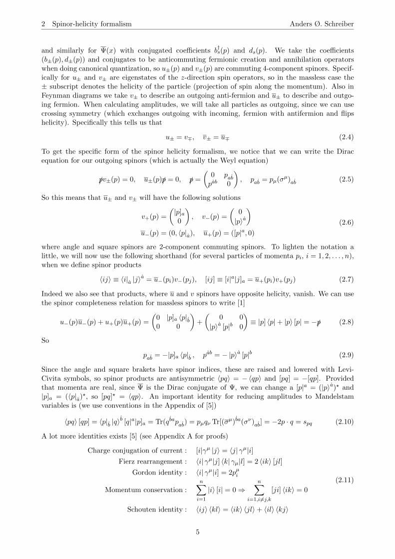
and similarly for Ψ(x) with conjugated coefficients b†s(p) and ds(p). We take the coefficients(b±(p), d±(p)) and conjugates to be anticommuting fermionic creation and annihilation operatorswhen doing canonical quantization, so u±(p) and v±(p) are commuting 4-component spinors. Specif-ically for u± and v± are eigenstates of the z-direction spin operators, so in the massless case the± subscript denotes the helicity of the particle (projection of spin along the momentum). Also inFeynman diagrams we take v± to describe an outgoing anti-fermion and u± to describe and outgo-ing fermion. When calculating amplitudes, we will take all particles as outgoing, since we can usecrossing symmetry (which exchanges outgoing with incoming, fermion with antifermion and flipshelicity). Specifically this tells us that

u± = v∓, v± = u∓ (2.4)

To get the specific form of the spinor helicity formalism, we notice that we can write the Diracequation for our outgoing spinors (which is actually the Weyl equation)

/pv±(p) = 0, u±(p)/p = 0, /p =

(0 pabpab 0

), pab = pµ(σµ)ab (2.5)

So this means that u± and v± will have the following solutions

v+(p) =

(|p]a0

), v−(p) =

(0

|p〉a)

u−(p) = (0, 〈p|a), u+(p) = ([p|a, 0)

(2.6)

where angle and square spinors are 2-component commuting spinors. To lighten the notation alittle, we will now use the following shorthand (for several particles of momenta pi, i = 1, 2, . . . , n),when we define spinor products

〈ij〉 ≡ 〈i|a |j〉a = u−(pi)v−(pj), [ij] ≡ [i|a|j]a = u+(pi)v+(pj) (2.7)

Indeed we also see that products, where u and v spinors have opposite helicity, vanish. We can usethe spinor completeness relation for massless spinors to write [1]

u−(p)u−(p) + u+(p)u+(p) =

(0 |p]a 〈p|b0 0

)+

(0 0

|p〉a [p|b 0

)≡ |p] 〈p|+ |p〉 [p| = −/p (2.8)

So

pab = −|p]a 〈p|b , pab = − |p〉a [p|b (2.9)

Since the angle and square brakets have spinor indices, these are raised and lowered with Levi-Civita symbols, so spinor products are antisymmetric 〈pq〉 = −〈qp〉 and [pq] = −[qp]. Providedthat momenta are real, since Ψ is the Dirac conjugate of Ψ, we can change a [p|a = (|p〉a)? and|p]a = (〈p|a)?, so [pq]? = 〈qp〉. An important identity for reducing amplitudes to Mandelstamvariables is (we use conventions in the Appendix of [5])

〈pq〉 [qp] = 〈p|b |q〉b [q|a|p]a = Tr(qbapab) = pµqν Tr[(σµ)ba(σν)ab] = −2p · q = spq (2.10)

A lot more identities exists [5] (see Appendix A for proofs)

Charge conjugation of current : [i|γµ |j〉 = 〈j| γµ|i]Fierz rearrangement : 〈i| γµ|j] 〈k| γµ|l] = 2 〈ik〉 [jl]

Gordon identity : 〈i| γµ|i] = 2pµi

Momentum conservation :

n∑i=1

|i〉 [i| = 0⇒n∑

i=1,i 6=j,k[ji] 〈ik〉 = 0

Schouten identity : 〈ij〉〈kl〉 = 〈ik〉〈jl〉+ 〈il〉〈kj〉

(2.11)

5

3 Color decomposition in SU(N) Gauge Theory Anders Ø. Schreiber

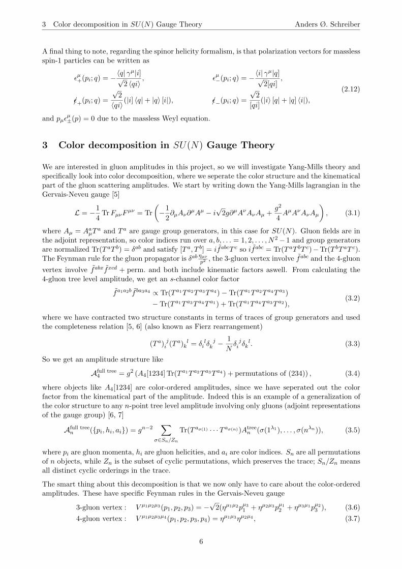
A final thing to note, regarding the spinor helicity formalism, is that polarization vectors for masslessspin-1 particles can be written as

εµ+(pi; q) = −〈q| γµ|i]√

2 〈qi〉,

/ε+(pi; q) =

√2

〈qi〉(|i] 〈q|+ |q〉 [i|),

εµ−(pi; q) = −〈i| γµ|q]√

2[qi],

/ε−(pi; q) =

√2

[qi](|i〉 [q|+ |q] 〈i|),

(2.12)

and pµεµ±(p) = 0 due to the massless Weyl equation.

3 Color decomposition in SU(N) Gauge Theory

We are interested in gluon amplitudes in this project, so we will investigate Yang-Mills theory andspecifically look into color decomposition, where we seperate the color structure and the kinematicalpart of the gluon scattering amplitudes. We start by writing down the Yang-Mills lagrangian in theGervais-Neveu gauge [5]

L = −1

4TrFµνF

µν = Tr

(−1

2∂µAν∂

µAµ − i√

2g∂µAνAνAµ +g2

4AµAνAνAµ

), (3.1)

where Aµ = AaµTa and T a are gauge group generators, in this case for SU(N). Gluon fields are in

the adjoint representation, so color indices run over a, b, . . . = 1, 2, . . . , N2− 1 and group generatorsare normalized Tr(T aT b) = δab and satisfy [T a, T b] = ifabcT c so ifabc = Tr(T aT bT c)−Tr(T bT aT c).The Feynman rule for the gluon propagator is δab

ηµνp2

, the 3-gluon vertex involve fabc and the 4-gluon

vertex involve fabxfxcd + perm. and both include kinematic factors aswell. From calculating the4-gluon tree level amplitude, we get an s-channel color factor

fa1a2bf ba3a4 ∝ Tr(T a1T a2T a3T a4)− Tr(T a1T a2T a4T a3)

− Tr(T a1T a3T a4T a1) + Tr(T a1T a4T a3T a2),(3.2)

where we have contracted two structure constants in terms of traces of group generators and usedthe completeness relation [5, 6] (also known as Fierz rearrangement)

(T a) ji (T a) lk = δ li δ

jk −

1

Nδ ji δ

lk . (3.3)

So we get an amplitude structure like

Afull tree4 = g2 (A4[1234] Tr(T a1T a2T a3T a4) + permutations of (234)) , (3.4)

where objects like A4[1234] are color-ordered amplitudes, since we have seperated out the colorfactor from the kinematical part of the amplitude. Indeed this is an example of a generalization ofthe color structure to any n-point tree level amplitude involving only gluons (adjoint representationsof the gauge group) [6, 7]

Afull treen ({pi, hi, ai}) = gn−2

∑σ∈Sn/Zn

Tr(T aσ(1) · · ·T aσ(n))Atreen (σ(1λ1), . . . , σ(nλn)), (3.5)

where pi are gluon momenta, hi are gluon helicities, and ai are color indices. Sn are all permutationsof n objects, while Zn is the subset of cyclic permutations, which preserves the trace; Sn/Zn meansall distinct cyclic orderings in the trace.

The smart thing about this decomposition is that we now only have to care about the color-orderedamplitudes. These have specific Feynman rules in the Gervais-Neveu gauge

3-gluon vertex : V µ1µ2µ3(p1, p2, p3) = −√

2(ηµ1µ2pµ31 + ηµ2µ3pµ12 + ηµ3µ1pµ23 ), (3.6)

4-gluon vertex : V µ1µ2µ3µ4(p1, p2, p3, p4) = ηµ1µ3ηµ2µ4 , (3.7)

6


and gluon propagator ηµν

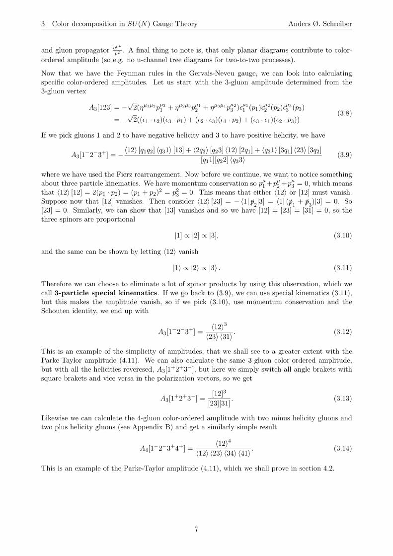
p2. A final thing to note is, that only planar diagrams contribute to color-

ordered amplitude (so e.g. no u-channel tree diagrams for two-to-two processes).

Now that we have the Feynman rules in the Gervais-Neveu gauge, we can look into calculatingspecific color-ordered amplitudes. Let us start with the 3-gluon amplitude determined from the3-gluon vertex

A3[123] = −√

2(ηµ1µ2pµ31 + ηµ2µ3pµ12 + ηµ3µ1pµ23 )εµ11 (p1)εµ22 (p2)ε

µ33 (p3)

= −√

2((ε1 · ε2)(ε3 · p1) + (ε2 · ε3)(ε1 · p2) + (ε3 · ε1)(ε2 · p3))(3.8)

If we pick gluons 1 and 2 to have negative helicity and 3 to have positive helicity, we have

A3[1−2−3+] = −〈12〉 [q1q2] 〈q31〉 [13] + 〈2q3〉 [q23] 〈12〉 [2q1] + 〈q31〉 [3q1] 〈23〉 [3q2]

[q11][q22] 〈q33〉(3.9)

where we have used the Fierz rearrangement. Now before we continue, we want to notice somethingabout three particle kinematics. We have momentum conservation so pµ1 +pµ2 +pµ3 = 0, which meansthat 〈12〉 [12] = 2(p1 · p2) = (p1 + p2)

2 = p23 = 0. This means that either 〈12〉 or [12] must vanish.Suppose now that [12] vanishes. Then consider 〈12〉 [23] = −〈1| /p2|3] = 〈1| (/p1 + /p3)|3] = 0. So[23] = 0. Similarly, we can show that [13] vanishes and so we have [12] = [23] = [31] = 0, so thethree spinors are proportional

|1] ∝ |2] ∝ |3], (3.10)

and the same can be shown by letting 〈12〉 vanish

|1〉 ∝ |2〉 ∝ |3〉 . (3.11)

Therefore we can choose to eliminate a lot of spinor products by using this observation, which wecall 3-particle special kinematics. If we go back to (3.9), we can use special kinematics (3.11),but this makes the amplitude vanish, so if we pick (3.10), use momentum conservation and theSchouten identity, we end up with

A3[1−2−3+] =

〈12〉3〈23〉〈31〉 . (3.12)

This is an example of the simplicity of amplitudes, that we shall see to a greater extent with theParke-Taylor amplitude (4.11). We can also calculate the same 3-gluon color-ordered amplitude,but with all the helicities reveresed, A3[1

+2+3−], but here we simply switch all angle brakets withsquare brakets and vice versa in the polarization vectors, so we get

A3[1+2+3−] =

[12]3

[23][31]. (3.13)

Likewise we can calculate the 4-gluon color-ordered amplitude with two minus helicity gluons andtwo plus helicity gluons (see Appendix B) and get a similarly simple result

A4[1−2−3+4+] =

〈12〉4〈12〉〈23〉〈34〉〈41〉 . (3.14)

This is an example of the Parke-Taylor amplitude (4.11), which we shall prove in section 4.2.

7


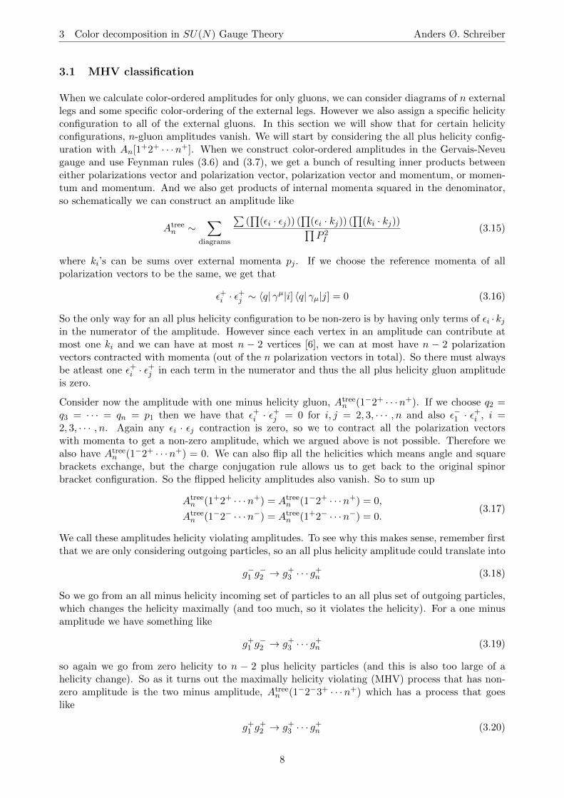
3.1 MHV classification

When we calculate color-ordered amplitudes for only gluons, we can consider diagrams of n externallegs and some specific color-ordering of the external legs. However we also assign a specific helicityconfiguration to all of the external gluons. In this section we will show that for certain helicityconfigurations, n-gluon amplitudes vanish. We will start by considering the all plus helicity config-uration with An[1+2+ · · ·n+]. When we construct color-ordered amplitudes in the Gervais-Neveugauge and use Feynman rules (3.6) and (3.7), we get a bunch of resulting inner products betweeneither polarizations vector and polarization vector, polarization vector and momentum, or momen-tum and momentum. And we also get products of internal momenta squared in the denominator,so schematically we can construct an amplitude like

Atreen ∼

∑diagrams

∑(∏

(εi · εj)) (∏

(εi · kj)) (∏

(ki · kj))∏P 2I

(3.15)

where ki’s can be sums over external momenta pj . If we choose the reference momenta of allpolarization vectors to be the same, we get that

ε+i · ε+j ∼ 〈q| γµ|i] 〈q| γµ|j] = 0 (3.16)

So the only way for an all plus helicity configuration to be non-zero is by having only terms of εi ·kjin the numerator of the amplitude. However since each vertex in an amplitude can contribute atmost one ki and we can have at most n − 2 vertices [6], we can at most have n − 2 polarizationvectors contracted with momenta (out of the n polarization vectors in total). So there must alwaysbe atleast one ε+i · ε+j in each term in the numerator and thus the all plus helicity gluon amplitudeis zero.

Consider now the amplitude with one minus helicity gluon, Atreen (1−2+ · · ·n+). If we choose q2 =

q3 = · · · = qn = p1 then we have that ε+i · ε+j = 0 for i, j = 2, 3, · · · , n and also ε−1 · ε+i , i =2, 3, · · · , n. Again any εi · εj contraction is zero, so we to contract all the polarization vectorswith momenta to get a non-zero amplitude, which we argued above is not possible. Therefore wealso have Atree

n (1−2+ · · ·n+) = 0. We can also flip all the helicities which means angle and squarebrackets exchange, but the charge conjugation rule allows us to get back to the original spinorbracket configuration. So the flipped helicity amplitudes also vanish. So to sum up

Atreen (1+2+ · · ·n+) = Atree

n (1−2+ · · ·n+) = 0,

Atreen (1−2− · · ·n−) = Atree

n (1+2− · · ·n−) = 0.(3.17)

We call these amplitudes helicity violating amplitudes. To see why this makes sense, remember firstthat we are only considering outgoing particles, so an all plus helicity amplitude could translate into

g−1 g−2 → g+3 · · · g+n (3.18)

So we go from an all minus helicity incoming set of particles to an all plus set of outgoing particles,which changes the helicity maximally (and too much, so it violates the helicity). For a one minusamplitude we have something like

g+1 g−2 → g+3 · · · g+n (3.19)

so again we go from zero helicity to n − 2 plus helicity particles (and this is also too large of ahelicity change). So as it turns out the maximally helicity violating (MHV) process that has non-zero amplitude is the two minus amplitude, Atree

n (1−2−3+ · · ·n+) which has a process that goeslike

g+1 g+2 → g+3 · · · g+n (3.20)

8

4 Recursion techniques Anders Ø. Schreiber

So here we only gain n− 4 extra plus helicities in the process (which turns out to be the maximalchange in helicity you can make). Furthermore, less helicity violating processes will be noted NMHV,N2MHV, . . ., NkMHV and so on, where NMHV has three minus and rest plus gluons, N2MHV hasfour minus and rest plus. We shall calculate the MHV amplitude (which is exactly the previouslymentioned Parke-Taylor amplitude, (4.11)) in the section 4.2 using the BCFW recursion relationsand an NMHV amplitude using a MHV vertex expansion in section 4.5.

4 Recursion techniques

In this section we will introduce methods of on-shell recursion relations, specifically BCFW recursionrelations and MHV vertex expansions (including the CSW prescription). Both of these methods arebased on the use of the complex plane, where we shift external particle momenta with a complexparameter.

Let us start by considering an on-shell amplitude An with n external particles of momenta p2i = 0,i = 1, 2, . . . , n. We take all particles to be outgoing, so momentum conservation implies

∑ni=1 p

µi = 0.

Now we want to shift the external momenta, because as we shall see, this will be a smart trick toevaluate amplitudes recursively. We introduce exactly n complex-valued vectors rµi such that

(i)∑n

i=1 rµi = 0,

(ii) ri · rj = 0, ∀i, j = 1, 2, . . . , n and in particular r2i = 0,

(iii) pi · ri = 0, ∀i = 1, 2, . . . , n.

Specifically we will use these n new vectors to shift momenta, introducing the hat notation for ashifted momentum

pµi ≡ pµi + zrµi , z ∈ C. (4.1)

The three conditions on rµi vectors now imply three conditions on pµi

(a)∑n

i=1 pµi = 0,

(b) p2i = 0, ∀i = 1, 2, . . . , n,

(c) For a non-trivial subset of generic momenta (a set of atleast two, and no more than n − 2momenta) {pµi }i∈I , define PµI =

∑i∈I p

µi and RµI =

∑i∈I r

µi , then P 2

I is linear in z

P 2I =

(∑i∈I

pi

)2

= P 2I + z2PI ·RI . (4.2)

Define now zI = − P 2I

2PI ·RI , then we can write

P 2I = −P

2I

zI(z − zI). (4.3)

The reason why we want to consider leg-shifts for amplitudes is that, by doing these leg-shifts, wehave constructed a holomorphic function in the complex plane, An(z), where we reconstruct theoriginal amplitude by setting z = 0, An = An(z = 0). Specializing to tree-level amplitudes, thestructure of the function An(z) is pretty simple. Indeed they are rational functions of momentaand there are no square roots, logarithms and so on as there are for loop diagrams. The analyticstructure of An(z) is captured by poles, which only appear from shifted propagators 1/P 2

I , where

PI is the sum of a non-trivial subset of momenta. By property (c) we then have that 1/P 2I has a

9


simple pole at z = zI , where for generic momenta P 2I 6= 0 so zI 6= 0. So the structure is that An(z)

has simple poles, from propagators, away from the origin z = 0.

Now if we consider the function An(z)z and integrate around a contour, that surrounds the simple

pole at the origin, then by the residue theorem, the residue associated with the pole at the origin isexactly the unshifted amplitude An = An(z = 0). Then we can deform the contour to capture allother poles, and by the residue theorem we get

An = Resz=0An(z)

z= −

∑zI

Resz=zIAn(z)

z+Bn, (4.4)

where we note that the sign on the right-hand side is due to the orientation change of the contoursaround the poles away from the origin. We also note that as we deform the contour out to infinity,

we get Bn, which is the possible pole of An(z)z at z → ∞. Indeed if we look at one of the zI -poles,

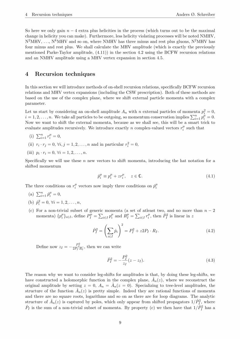
these are where the propagator 1/P 2I goes on-shell. Here a factorization happens near the pole

An(z)→ AL(zI)1

P 2I

AR(zI) = − zIz − zI

AL(zI)1

P 2I

AR(zI). (4.5)

So this means that

− Resz=zIAn(z)

z= AL(zI)

1

P 2I

AR(zI) = L R

PI

∧

∧

∧

∧

∧

∧

. (4.6)

Now why is this useful? Well now we can take an n-point amplitude and factorize it into ”lessthan n”-point amplitudes and thus we actually have a way of recursively calculating amplitudes attree-level. Before we write down the full general recursion relation, we note that the Bn term doesnot in general have an expression for it. However in most cases one proves (or assumes) that Bn iszero, or even stronger, one shows that

An(z)→ 0, z →∞. (4.7)

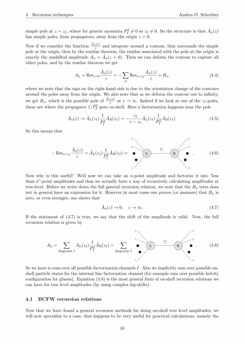
If the statement of (4.7) is true, we say that the shift of the amplitude is valid. Now, the fullrecursion relation is given by

An =∑

diagrams I

AL(zI)1

P 2I

AR(zI) =∑

diagrams I

L R

PI

∧

∧

∧

∧

∧

∧

. (4.8)

So we have to sum over all possible factorization channels I. Also we implicitly sum over possible on-shell particle states for the internal line factorzation channel (for example sum over possible helcityconfiguration for gluons). Equation (4.8) is the most general form of on-shell recursion relations wecan have for tree level amplitudes (by using complex leg-shifts).

4.1 BCFW recursion relations

Now that we have found a general recursion methods for doing on-shell tree level amplitudes, wewill now specialize to a case, that happens to be very useful for practical calculations, namely the

10


BCFW recursion relations. For BCFW we shift only two of the legs, i and j and the rest of the legsare unshifted (take rµk = 0, for k 6= i, j). We implement this shift on angle and square spinors by

|i] = |i] + z|j], |j] = |j], |i〉 = |i〉 , |j〉 = |j〉 − z |i〉 , (4.9)

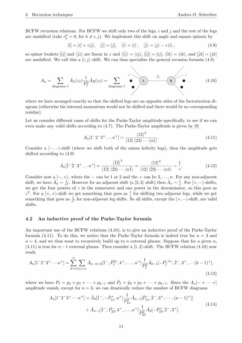
so spinor brakets [ij] and 〈ji〉 are linear in z and 〈ij〉 = 〈ij〉, [ij] = [ij], 〈ik〉 = 〈ik〉, and [jk] = [jk]are unshifted. We call this a [i, j〉 shift. We can thus specialize the general recusion formula (4.8)

An =∑

diagrams I

AL(zI)1

P 2I

AR(zI) =∑

diagrams I

L R

PIji

. (4.10)

where we have arranged exactly so that the shifted legs are on opposite sides of the factorization di-agram (otherwise the internal momentum would not be shifted and there would be no correspondingresidue).

Let us consider different cases of shifts for the Parke-Taylor amplitude specifically, to see if we caneven make any valid shifts according to (4.7). The Parke-Taylor amplitude is given by [8]

An[1−2−3+ . . . n+] =〈12〉4

〈12〉〈23〉 · · · 〈n1〉 . (4.11)

Consider a [−,−〉-shift (where we shift both of the minus helicity legs), then the amplitude getsshifted according to (4.9)

An[1−2−3+ . . . n+] =〈12〉4

〈12〉〈23〉 · · · 〈n1〉=

〈12〉4〈12〉〈23〉 · · · 〈n1〉

∼ 1

z. (4.12)

Consider now a [−,+〉, where the − can be 1 or 2 and the + can be 3, . . . , n. For any non-adjacentshift, we have An ∼ 1

z2. However for an adjacent shift (a [2, 3〉 shift) then An ∼ 1

z . For [+,−〉-shifts,we get the four powers of z in the numerator and one power in the denominator, so this goes asz3. For a [+,+〉-shift we get something that goes as 1

z for shifting two adjacent legs, while we getsomething that goes as 1

z2for non-adjacent leg shifts. So all shifts, except the [+,−〉-shift, are valid

shifts.

4.2 An inductive proof of the Parke-Taylor formula

An important use of the BCFW relations (4.10), is to give an inductive proof of the Parke-Taylorformula (4.11). To do this, we notice that the Parke-Taylor formula is indeed true for n = 3 andn = 4, and we thus want to recursively build up to n external gluons. Suppose that for a given n,(4.11) is true for n− 1 external gluons. Then consider a [1, 2〉-shift. The BCFW relation (4.10) nowreads

An[1−2−3+ · · ·n+] =

n∑k=4

∑hI=±

An−k+3[1−, P hII , k+, . . . , n+]

1

P 2I

Ak−1[−P−hII , 2−, 3+, . . . (k − 1)+],

(4.13)

where we have PI = p2 + p3 + · · · + pk−1 and PI = p2 + p3 + · · · + pk−1. Since the An[− + · · ·+]amplitude vanish, except for n = 3, we can drastically reduce the number of BCFW diagrams

An[1−2−3+ · · ·n+] = A3[1−,−P+

1n, n+]

1

P 21n

An−1[P−1n, 2

−, 3+, · · · , (n− 1)+]]

+ An−1[1−, P−23, 4

+, . . . , n+]1

P 223

A3[−P+23, 2

−, 3+].

(4.14)

11


where Pij = pi + pj and PI is evaluated at the residue value where z = zI , such that the propagatorgoes on-shell, P 2

I = 0. Consider now the 3-point anti-MHV amplitude in the first line of (4.14),

A3[1−,−P+

1n, n+]. We have shown in section 3, that it has the form

A3[1−,−P+

1n, n+] =

[P1nn]3

[n1][1P1n], (4.15)

where we have chosen the convention [5] for analytic continuation of angle and square brackets|−p〉 = − |p〉 and |−p] = |p]. If we use the on-shell condition for the internal line, it is possible to showthat [1n] = 0. The numerator in (4.15) also vanishes, as we can show that |P1n〉 [P1nn] = |1〉 [1n] = 0.Similarly [1P1n] = 0. So all spinor products in (4.15) vanish, but since we have three powers of spinorproducts in the numerator and two in the denominator, so we conclude that A3[1

−,−P+1n, n

+] = 0.We are now left with

An[1−2−3+ · · ·n+] = An−1[1−, P−23, 4

+, . . . , n+]1

P 223

A3[−P+23, 2

−, 3+]. (4.16)

The 3-point anti-MHV amplitude we are left with does not vanish, since the leg 2 shift is on anangle bracket, so we cannot use momentum conservation to make this amplitude vanish. Now wecan write down the explicit expression for the amplitudes on the righthand side of (4.16)

An[1−2−3+ · · ·n+] =〈1P23〉

3

〈P234〉〈45〉 · · · 〈n1〉× 1

〈23〉 [23]× [3P23]

3

[P232][23](4.17)

We wish to eliminate the spinor products including P23, which is possible since 〈1P23〉 [3P23] =−〈12〉 [23] and 〈P234〉 [P232] = −〈34〉 [23]. We then get our final result

An[1−2−3+ · · ·n+] =〈12〉4

〈12〉〈23〉〈34〉〈45〉 · · · 〈n1〉 , (4.18)

which by induction proves the validity of the Parke-Taylor formula.

This proof can also be generalized to non-adjacent legs, say legs i and j have negative helicity (withan [i, j〉 shift, which can also be checked to be valid), while the rest of the legs have positive helicity.Then we have

An[1+ · · · i− · · · j− · · ·n+] = A3 [i−,−P+

i−1,i, (i− 1)+]1

P 2i−1,i

An−1[P−i−1,i, (i+ 1)+, . . . , j−, . . . , (i− 2)+]

+ An−1 [i−, P−j,j+1, (j + 2)+, . . . , (i− 1)+]

1

P 2j,j+1

A3[−P+j,j+1, j

−, (j + 1)+].

(4.19)

The amplitude A3 [i−,−P+

i−1,i, (i − 1)+] will vanish, since P 2i−1,i = 〈i− 1, i〉 [i − 1, i] = 0, and

A3[−P+j,j+1, j

−, (j + 1)+] will not since only the j angle spinor is shifted. So

An[1+ · · · i− · · · j− · · ·n+] =〈ij〉4

〈12〉 · · · 〈ij〉 · · · 〈n1〉 . (4.20)

which matches the form of the adjacent leg Parke-Taylor amplitude (4.11).

4.3 The 4-graviton amplitude and KLT relations

An interesting example of the use of the BCFW recursion relations is to calculate graviton ampli-tudes and explore the so-called KLT relations [9]. To calculate graviton amplitudes, we first wantto consider the action of general relativity, the Einstein-Hilbert action

SEH =1

2κ2

∫d4x√−gR (4.21)

12


where κ2 = 8πGN . However this action happens to inherit a huge problem from considering aperturbation around the Minkowski metric. We introduce the graviton field as this perturbationgµν = ηµν + κhµν [5]. Then the expansion of

√−g contains an infinite number of vertices involvingtwo derivatives and n fields hµν . So we get very complicated Feynman rules for Einstein gravity.However gravitons are spin-2 particles and in 4 spacetime dimensions they have helicity ±2 [5]. Thisinformation makes us able to use a trick to calculate gravition amplitudes using BCFW relations,because we can determine the 3-point graviton amplitude, for a given helicity configuration, fromlittle group scaling (see Appendix C).

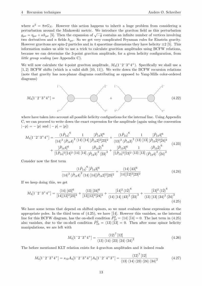
We will now calculate the 4-point graviton amplitude, M4(1−2−3+4+). Specifically we shall use a

[1, 2〉 BCFW shifts (which is a valid shift [10, 11]). We write down the BCFW recursion relations(note that gravity has non-planar diagrams contributing as opposed to Yang-Mills color-ordereddiagrams)

M4[1−2−3+4+] =

1− 2−

3+4+

+

1− 2−

4+3+

(4.22)

where have taken into account all possible helicity configuations for the internal line. Using AppendixC, we can proceed to write down the exact expression for the amplitude (again using the convention|−p〉 = − |p〉 and | − p] = |p])

M4[1−2−3+4+] =

〈1P14〉6

〈14〉2 〈P144〉2

1

〈14〉 [14]

[P143]6

[P142]2[23]2+

〈1P13〉6

〈13〉2 〈P133〉2

1

〈13〉 [13]

[P134]6

[P132]2[24]2

+[P144]6

[1P14]2[14]21

〈14〉 [14]

〈P142〉6

〈P143〉2 〈23〉2

+[P133]6

[1P13]2[13]21

〈13〉 [13]

〈P132〉6

〈P134〉2 〈24〉2

(4.23)

Consider now the first term

〈1P14〉6

[P143]6

〈14〉2 〈P144〉2 〈14〉 [14][P142]2[23]2

=〈14〉 [43]6

[14][12]2[23]2(4.24)

If we keep doing this, we get

M4[1−2−3+4+] =

〈14〉 [43]6

[14][12]2[23]2+〈13〉 [34]6

[13][12]2[24]2+

[14]2 〈12〉6

〈14〉 [14] 〈43〉2 〈23〉2+

[13]2 〈12〉6

〈13〉 [13] 〈34〉2 〈24〉2(4.25)

We have some terms that depend on shifted spinors, so we must evaluate these expressions at theappropriate poles. In the third term of (4.25), we have [14]. However this vanishes, as the internalline for this BCFW diagram, has the on-shell condition P 2

14 = 〈14〉 [14] = 0. The last term in (4.25)also vanishes, due to the on-shell condition P 2

13 = 〈13〉 [13] = 0. Then after some spinor helicitymanipulations, we are left with

M4[1−2−3+4+] =

〈12〉7 [12]

〈13〉〈14〉〈23〉〈24〉〈34〉2(4.26)

The before mentioned KLT relation exists for 4-graviton amplitudes and it indeed reads

M4[1−2−3+4+] = s12A4[1

−2−3+4+]A4[1−2−4+3+] =

〈12〉7 [12]

〈13〉〈14〉〈23〉〈24〉〈34〉2(4.27)

13


This is an example of an extensive set of relations between gauge theory and gravity, which havebeen explored more comprehensively in [12]. This example also shows the simplicity of going throughthe BCFW recursion relations as compared to using Feynman diagrams [13]. Indeed a very explicitshowcase of the power of recursion methods.

4.4 Multi leg shift

So far we have only worked with a special case of the general recursion relations (4.8), where onlytwo of the legs are shifted, the BCFW recursion relations (4.10). We now want to try to involveshifts on more than just two legs and see if these can be useful. Consider the square spinor shift

|i] = |i] + zci|X], |i〉 = |i〉 (4.28)

where |X] is an arbitrary reference spinor and coefficient ci satisfy∑n

i=1 ci |i〉 = 0. In general this isknown as a multi-leg shift and for all ci 6= 0 it is an all-leg shift. A specific realization of a multi-legshift is the Risager shift [14] where c1 = 〈23〉, c2 = 〈31〉, and c3 〈12〉 while ci = 0 for i = 4, . . . , n.

An all-leg shift is useful for calculating NkMHV gluon tree amplitudes, as it can be shown that, underan all-leg shift, these go as 1/zk [15]. Therefore we can determine all gluon tree-level amplitudesthrough all-leg shift recursion relations (except MHV amplitudes, but we have already determinedthese with the Parke-Taylor formula).

4.5 MHV vertex expansion and the 6-gluon NMHV amplitude

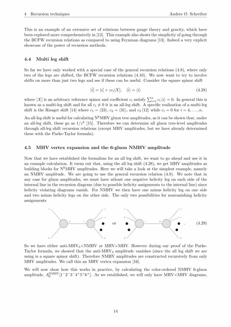
Now that we have established the formalism for an all leg shift, we want to go ahead and use it inan example calculation. It turns out that, using the all leg shift (4.28), we get MHV amplitudes asbuilding blocks for NkMHV amplitudes. Here we will take a look at the simplest example, namelyan NMHV amplitude. We are going to use the general recursion relation (4.8). We note that inany case for gluon amplitudes, we must have atleast one negative helicity leg on each side of theinternal line in the recursion diagram (due to possible helicity assignments to the internal line) sincehelicity violating diagrams vanish. For NMHV we then have one minus helicity leg on one sideand two minus helicity legs on the other side. The only two possibilities for nonvanishing helicityassignments

−

+

+ −

−

−

+

or −

−

+

+ +

−

−

+ . (4.29)

So we have either anti-MHV3×NMHV or MHV×MHV. However during our proof of the Parke-Taylor formula, we showed that the anti-MHV3 amplitude vanishes (since the all leg shift we areusing is a square spinor shift). Therefore NMHV amplitudes are constructed recursively from onlyMHV amplitudes. We call this an MHV vertex expansion [16].

We will now show how this works in practice, by calculating the color-ordered NMHV 6-gluonamplitude, ANMHV

6 [1−2−3−4+5+6+]. As we established, we will only have MHV×MHV diagrams,

14


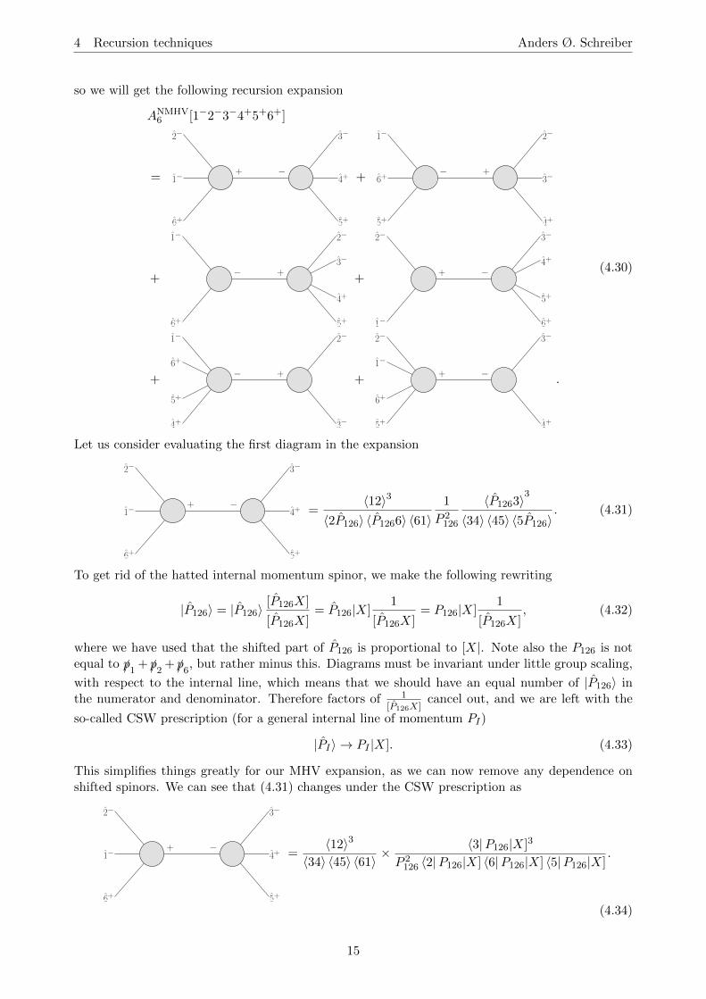
so we will get the following recursion expansion

ANMHV6 [1−2−3−4+5+6+]

=+ −

1−

2− 3−

4+

5+6+

+− +

6+

1− 2−

3−

4+5+

+− +

1− 2−

5+6+

3−

4+

++ −

2− 3−

6+1−

4+

5+

+− +

1− 2−

3−4+

5+

6+

++ −

2− 3−

4+5+

6+

1−

.

(4.30)

Let us consider evaluating the first diagram in the expansion

+ −1−

2− 3−

4+

5+6+

=〈12〉3

〈2P126〉〈P1266〉〈61〉1

P 2126

〈P1263〉3

〈34〉〈45〉〈5P126〉. (4.31)

To get rid of the hatted internal momentum spinor, we make the following rewriting

|P126〉 = |P126〉[P126X]

[P126X]= P126|X]

1

[P126X]= P126|X]

1

[P126X], (4.32)

where we have used that the shifted part of P126 is proportional to [X|. Note also the P126 is notequal to /p1 + /p2 + /p6, but rather minus this. Diagrams must be invariant under little group scaling,

with respect to the internal line, which means that we should have an equal number of |P126〉 inthe numerator and denominator. Therefore factors of 1

[P126X]cancel out, and we are left with the

so-called CSW prescription (for a general internal line of momentum PI)

|PI〉 → PI |X]. (4.33)

This simplifies things greatly for our MHV expansion, as we can now remove any dependence onshifted spinors. We can see that (4.31) changes under the CSW prescription as

+ −1−

2− 3−

4+

5+6+

=〈12〉3

〈34〉〈45〉〈61〉 ×〈3|P126|X]3

P 2126 〈2|P126|X] 〈6|P126|X] 〈5|P126|X]

.

(4.34)

15

5 Summary and outlook Anders Ø. Schreiber

By evaluating the rest of the diagrams in (4.30) and make good choices of reference spinors, tomake as many of the diagrams as possible vanish, then the resulting amplitude can be shown to beequivalent to

ANMHV6 [1−2−3−4+5+6+] =

〈3|P12|6]3

P 2126[21][16] 〈34〉〈45〉〈5|P16|2]

+〈1|P56|4]3

P 2156[23][34] 〈56〉〈61〉〈5|P16|2]

,

(4.35)

which is the expected result for this amplitude (see [5], eq. (3.34)).

We also want to note, that it might seem like the final amplitude depends on the reference spinor|X], as this can be chosen freely, however we are safe as Cauchy’s theorem makes us sure, thatby using any recursion relation with a shifted leg, we always end up back at the real amplitudeevaluating diagrams at the appropriate poles. So any reference spinor will make us arrive at theright amplitude.

5 Summary and outlook

In this project we have explored various aspects of scattering amplitudes and how to calculate them.In section 2 we derived the spinor-helicity formalism, which is very useful for expressing scatteringamplitudes, in a very simple form, in terms of spinor products and Mandelstam invariants.

In section 3 we presented the SU(N) Yang-Mills lagrangian and showed how color decompositionworks, where we seperate amplitudes involving color into a color part and a color-ordered amplitude(independent of color). We also derived how certain helicity configurations make color-orderedamplitudes vanish and thus introduced the MHV classification of color-ordered amplitudes.

The main content of this project is in section 4, where we explored different recursion techniques.Initially we introduced a general recursion relation based on complex momentum shifts of externalparticle momenta. Then we specialized to the BCFW recursion relations with only two externalmomenta being shifted. Then we showed the power of the BCFW relations by making an inductiveproof of the Parke-Taylor formula

Atreen [· · · i− · · · j− · · · ] =

〈ij〉4〈12〉 · · · 〈n1〉 , (5.1)

and by showing an example of the KLT relations between graviton and gluon amplitudes

M4[1−2−3+4+] = s12A4[1

−2−3+4+]A4[1−2−4+3+]. (5.2)

Finally we considered multi leg shifts and the MHV vertex expansion, with the specific example ofexpanding an 6-gluon NMHV amplitude in terms of MHV vertices only, as well as how the CSWprescription works. We also saw that we can choose any reference spinor for the multi leg shift, asthe resulting amplitude is independent of this choice due to Cauchy’s theorem.

The techniques presented in this project could be extended to one loop or maybe higher looplevel amplitudes. This has been explored in [5]. One could also consider extending the recursiontechniques to other types of theories, say the Standard Model. For some specific models involvingthe Higgs, and gluons or partons, this has been explored in [17, 18].

16

6 Appendix A: Proof of spinor helicity identities Anders Ø. Schreiber

6 Appendix A: Proof of spinor helicity identities

Here we make a proof of the remaining spinor helicity identites showcased in the spinor helicitysection, equation (2.11). We start from the top

Charge conjugation of current : [i|γµ |j〉 = 〈j| γµ|i] (6.1)

This identity can easily be realized through the following manipulation of spinor indices

[i|γµ |j〉 = ([i|a, 0)

(0 (σµ)ab

(σµ)ab 0

)(0

|j〉b

)= εbdεbc 〈j|d (σµ)ab|i]c = 〈j|d (σµ)dc|i]c = 〈j| γµ|i] (6.2)

which verifies the identity.

Fierz rearrangement : 〈i| γµ|j] 〈k| γµ|l] = 2 〈ik〉 [jl] (6.3)

We will show this by manipulating spinor indices

〈i| γµ|j] 〈k| γµ|l] = 〈i|a (σµ)ab|j]b 〈k|c (σµ)cd|l]d= −2εacεbd 〈i|a |j]b 〈k|c |l]d= 2εacεdb 〈i|a |j]b 〈k|c |l]d= 2 〈i|a |k〉a [j|d|l]d= 2 〈ik〉 [jl]

(6.4)


Gordon identity : 〈i| γµ|i] = 2pµi (6.5)

Consider again the spinor index manipulation

〈i| γµ|i] = 〈i|a (σµ)ab|i]b = (σµ)ab|i]b 〈i|a = −(σµ)ab(pi)ba = −pνi Tr((σµ)(σν)) = 2pµi (6.6)


Momentum conservation :

n∑i=1

|i〉 [i| = 0⇒n∑

i=1,i 6=j,k[ji] 〈ik〉 = 0 (6.7)

This identity holds from momentum conservation. If we have n momenta that sums to zero

n∑i=1

pµi = 0⇔n∑i=1

pµi (σµ)ab = −n∑i=1

|i]a 〈i|b = 0

We can also contract with σ to get

n∑i=1

|i〉a [i|b = 0 (6.8)

And indeed if j, k 6= i then

n∑i=1

[ji] 〈ik〉 = 0 (6.9)

17

6 Appendix A: Proof of spinor helicity identities Anders Ø. Schreiber

and when j, k = i then spinor products are trivially zero due to antisymmetry.

Schouten identity : 〈ij〉〈kl〉 = 〈ik〉〈jl〉+ 〈il〉〈kj〉 (6.10)

This identity can be shown from the fact that spinor brakets only have two components. So say wehave three two-component spinors, |i〉, |j〉, and |k〉, then we must be able to express one of them asa linear combination of the two others

|k〉 = a |i〉+ b |j〉 , (6.11)

then a = 〈jk〉〈ji〉 and b = 〈ik〉

〈ij〉 , so

|k〉 − a |i〉 − b |j〉 = |k〉+〈jk〉〈ij〉 |i〉+

〈ki〉〈ij〉 |j〉 = 0⇔ |k〉〈ij〉+ |i〉〈jk〉+ |j〉〈ki〉 = 0 (6.12)

or with some fourth spinor 〈l|

〈lk〉〈ij〉+ 〈li〉〈jk〉+ 〈lj〉〈ki〉 = 0 (6.13)

which is equivalent to the given identity.

18

7 Appendix B: The 4-gluon color-ordered MHV amplitude Anders Ø. Schreiber

7 Appendix B: The 4-gluon color-ordered MHV amplitude

In this appendix, we will showcase the full calculation of the color-ordered 4-gluon amplitude withtwo minus helicity gluons and two plus helicity gluons. Specifically we want to calculate the ampli-tude A4[1

−2−3+4+]. Now there are going to be three color-ordered Feynman diagrams contributingto this process, namely

A4[1−2−3+4+] =

1− 2−

3+4+

+

1− 2−

3+4+

+

4+ 3+

2−1−

(7.1)

We use the color-ordered Feynman rules (3.6) and (3.7)

A4[1−2−3+4+] = (ε1 · ε3)(ε2 · ε4)

+ 2εµ1(p1)εµ4(p4)(ηµ1µ4pρ1 + ηµ4ρpµ14 − ηρµ1(p1 + p4)

µ4)ηρσ

(p1 + p4)2

× (ησµ2(p1 + p4)µ3 + ηµ2µ3pσ2 + ηµ3σpµ23 )εµ2(p2)εµ3(p3)

+ 2εµ1(p1)εµ2(p2)(ηµ1µ2pρ1 + ηµ2ρpµ12 − ηρµ1(p1 + p2)

µ2)ηρσ

(p1 + p2)2

× (ησµ3(p1 + p2)µ4 + ηµ3µ4pσ3 + ηµ4σpµ34 )εµ3(p3)εµ4(p4)

= (ε1 · ε3)(ε2 · ε4)

+ 2((ε1 · ε4)p1σ + ε4σ(p4 · ε1)− ε1σ(p1 · ε4 + p4 · ε4))1

(p1 + p4)2

× (εσ2 (p1 · ε3 + p4 · ε3) + (ε2 · ε3)pσ2 + εσ3 (p3 · ε2))

+ 2((ε1 · ε2)p1σ + ε2σ(p2 · ε1)− ε1σ(p1 · ε2 + p2 · ε2))1

(p1 + p2)2

× (εσ3 (p1 · ε4 + p2 · ε4) + (ε3 · ε4)pσ3 + εσ4 (p4 · ε3))= (ε1 · ε3)(ε2 · ε4)

+ 21

(p1 + p4)2[(ε1 · ε4)(p1 · ε2)(p1 · ε3) + (ε1 · ε4)(p1 · ε2)(p4 · ε3) + (ε1 · ε4)(ε2 · ε3)(p1 · p2)

+ (ε1 · ε4)(p1 · ε3)(p3 · ε2) + (ε2 · ε4)(p4 · ε1)(p1 · ε3) + (ε2 · ε4)(p4 · ε1)(p4 · ε3)+ (p2 · ε4)(p4 · ε1)(ε2 · ε3) + (ε3 · ε4)(p4 · ε1)(p3 · ε2)− (ε1 · ε2)(p1 · ε4)(p1 · ε3)− (ε1 · ε2)(p4 · ε4)(p1 · ε3)− (ε1 · ε2)(p1 · ε4)(p4 · ε3)− (ε1 · ε2)(p4 · ε4)(p4 · ε3)− (p2 · ε1)(p1 · ε4)(ε2 · ε3)− (p2 · ε1)(p4 · ε4)(ε2 · ε3)− (ε1 · ε3)(p1 · ε4)(p3 · ε2)− (ε1 · ε3)(p4 · ε4)(p3 · ε2)]

+ 21

(p1 + p2)2[(ε1 · ε2)(p1 · ε3)(p1 · ε4) + (ε1 · ε2)(p1 · ε3)(p2 · ε4) + (ε1 · ε2)(p1 · p3)(ε3 · ε4)

+ (ε1 · ε2)(p1 · ε4)(p4 · ε3) + (ε2 · ε3)(p2 · ε1)(p1 · ε4) + (ε2 · ε3)(p2 · ε1)(p2 · ε4)+ (p3 · ε2)(p2 · ε1)(ε3 · ε4) + (ε2 · ε4)(p2 · ε1)(p4 · ε3)− (ε1 · ε3)(p1 · ε2)(p1 · ε4)− (ε1 · ε3)(p1 · ε2)(p2 · ε4)− (ε1 · ε3)(p2 · ε2)(p1 · ε4)− (ε1 · ε3)(p2 · ε2)(p2 · ε4)− (p3 · ε1)(p1 · ε2)(ε3 · ε4)− (p3 · ε1)(p2 · ε2)(ε3 · ε4)− (ε1 · ε4)(p1 · ε2)(p4 · ε3)− (ε1 · ε4)(p2 · ε2)(p4 · ε3)]

19


= (ε1 · ε3)(ε2 · ε4)

+ 21

(p1 + p4)2[(ε1 · ε4)(p1 · ε2)(p1 · ε3) + (ε1 · ε4)(p1 · ε2)(p4 · ε3) + (ε1 · ε4)(ε2 · ε3)(p1 · p2)

+ (ε1 · ε4)(p1 · ε3)(p3 · ε2) + (ε2 · ε4)(p4 · ε1)(p1 · ε3) + (ε2 · ε4)(p4 · ε1)(p4 · ε3)+ (p2 · ε4)(p4 · ε1)(ε2 · ε3) + (ε3 · ε4)(p4 · ε1)(p3 · ε2)− (ε1 · ε2)(p1 · ε4)(p1 · ε3)− (ε1 · ε2)(p1 · ε4)(p4 · ε3)− (p2 · ε1)(p1 · ε4)(ε2 · ε3)− (ε1 · ε3)(p1 · ε4)(p3 · ε2)]

+ 21

(p1 + p2)2[(ε1 · ε2)(p1 · ε3)(p1 · ε4) + (ε1 · ε2)(p1 · ε3)(p2 · ε4) + (ε1 · ε2)(p1 · p3)(ε3 · ε4)

+ (ε1 · ε2)(p1 · ε4)(p4 · ε3) + (ε2 · ε3)(p2 · ε1)(p1 · ε4) + (ε2 · ε3)(p2 · ε1)(p2 · ε4)+ (p3 · ε2)(p2 · ε1)(ε3 · ε4) + (ε2 · ε4)(p2 · ε1)(p4 · ε3)− (ε1 · ε3)(p1 · ε2)(p1 · ε4)− (ε1 · ε3)(p1 · ε2)(p2 · ε4)− (p3 · ε1)(p1 · ε2)(ε3 · ε4)− (ε1 · ε4)(p1 · ε2)(p4 · ε3)].

We can now insert spinor helicity expressions

A4[1−2−3+4+] =

〈1| γµ|q1] 〈q3| γµ|3] 〈2| γν |q2] 〈q4| γν |4] 〈12〉 [12] 〈14〉 [14]

4 〈12〉 [12] 〈14〉 [14][q11][q22] 〈q33〉〈q44〉

+〈12〉 [12]

2 〈12〉 [12] 〈14〉 [14][q11][q22] 〈q33〉〈q44〉× {〈1| γµ|q1] 〈q4| γµ|4] 〈2| /p1|q2] 〈q3| /p1|3] + 〈1| γµ|q1] 〈q4| γµ|4] 〈2| /p1|q2] 〈q3| /p4|3]

+ 〈1| γµ|q1] 〈q4| γµ|4] 〈2| γν |q2] 〈q3| γν |3](p1 · p2) + 〈1| γµ|q1] 〈q4| γµ|4] 〈q3| /p1|3] 〈2| /p3|q2]+ 〈2| γµ|q2] 〈q4| γµ|4] 〈1| /p4|q1] 〈q3| /p1|3] + 〈2| γµ|q2] 〈q4| γµ|4] 〈1| /p4|q1] 〈q3| /p4|3]

+ 〈2| γµ|q2] 〈q3| γµ|3] 〈1| /p4|q1] 〈q4| /p2|4] + 〈q3| γµ|3] 〈q4| γµ|4] 〈1| /p4|q1] 〈2| /p3|q2]− 〈1| γµ|q1] 〈2| γµ|q2] 〈q4| /p1|4] 〈q3| /p1|3]− 〈1| γµ|q1] 〈2| γµ|q2] 〈q4| /p1|4] 〈q3| /p4|3]

− 〈2| γµ|q2] 〈q3| γµ|3] 〈1| /p2|q1] 〈q4| /p1|4]− 〈1| γµ|q1] 〈q3| γµ|3] 〈q4| /p1|4] 〈2| /p3|q2]}

+〈14〉 [14]

2 〈12〉 [12] 〈14〉 [14][q11][q22] 〈q33〉〈q44〉× {〈1| γµ|q1] 〈2| γµ|q2] 〈q3| /p1|3] 〈q4| /p1|4] + 〈1| γµ|q1] 〈2| γµ|q2] 〈q3| /p1|3] 〈q4| /p2|4]

+ 〈1| γµ|q1] 〈2| γµ|q2] 〈q3| γν |3] 〈q4| γν |4](p1 · p3) + 〈1| γµ|q1] 〈2| γµ|q2] 〈q4| /p1|4] 〈q3| /p4|3]

+ 〈2| γµ|q2] 〈q3| γµ|3] 〈1| /p2|q1] 〈q4| /p2|4] + 〈2| γµ|q2] 〈q3| γµ|3] 〈1| /p2|q1] 〈q4| /p2|4]

+ 〈q3| γµ|3] 〈q4| γµ|4] 〈2| /p3|q2] 〈1| /p2|q1] + 〈2| γµ|q2] 〈q4| γµ|4] 〈1| /p2|q1] 〈q3| /p4|3]

− 〈1| γµ|q1] 〈q3| γµ|3] 〈2| /p1|q2] 〈q4| /p1|4]− 〈1| γµ|q1] 〈q3| γµ|3] 〈2| /p1|q2] 〈q4| /p2|4]

− 〈q3| γµ|3] 〈q4| γµ|4] 〈1| /p3|q1] 〈2| /p1|q2]− 〈1| γµ|q1] 〈q4| γµ|4] 〈2| /p1|q2] 〈q3| /p4|3]}.

We can now Fierz rearrange and insert spinor helicity quantities for /p

A4[1−2−3+4+] =

1

〈12〉 [12] 〈14〉 [14][q11][q22] 〈q33〉〈q44〉{〈1q3〉 [q13] 〈2q4〉 [q24] 〈12〉 [12] 〈14〉 [14]

+ 〈1q4〉 [q14] 〈21〉 [1q2] 〈q31〉 [13] 〈12〉 [12] + 〈1q4〉 [q14] 〈21〉 [1q2] 〈q34〉 [43] 〈12〉 [12]

+ 〈1q4〉 [q14] 〈2q3〉 [q23] 〈12〉 [12] 〈12〉 [12] + 〈1q4〉 [q14] 〈q31〉 [13] 〈23〉 [3q2] 〈12〉 [12]

+ 〈2q4〉 [q24] 〈14〉 [4q1] 〈q31〉 [13] 〈12〉 [12] + 〈2q4〉 [q24] 〈14〉 [4q1] 〈q34〉 [43] 〈12〉 [12]

+ 〈2q3〉 [q23] 〈14〉 [4q1] 〈q42〉 [24] 〈12〉 [12] + 〈q3q4〉 [34] 〈14〉 [4q1] 〈23〉 [3q2] 〈12〉 [12]

− 〈12〉 [q1q2] 〈q41〉 [14] 〈q31〉 [13] 〈12〉 [12]− 〈12〉 [q1q2] 〈q41〉 [14] 〈q34〉 [43] 〈12〉 [12]

− 〈2q3〉 [q23] 〈12〉 [2q1] 〈q41〉 [14] 〈12〉 [12]− 〈1q3〉 [q13] 〈q41〉 [14] 〈23〉 [3q2] 〈12〉 [12]

+ 〈12〉 [q1q2] 〈q31| [13] 〈q41〉 [14] 〈14〉 [14] + 〈12〉 [q1q2] 〈q31〉 [13] 〈q42〉 [24] 〈14〉 [14]

20


+ 〈12〉 [q1q2] 〈q3q4〉 [34] 〈14〉 [14] 〈13〉 [13] + 〈12〉 [q1q2] 〈q41〉 [14] 〈q34〉 [43] 〈14〉 [14]

+ 〈2q3〉 [q23] 〈12〉 [2q1] 〈q42〉 [24] 〈14〉 [14] + 〈2q3〉 [q23] 〈12〉 [2q1] 〈q42〉 [24] 〈14〉 [14]

+ 〈q3q4〉 [34] 〈23〉 [3q2] 〈12〉 [2q1] 〈14〉 [14] + 〈2q4〉 [24] 〈12〉 [2q1] 〈q34〉 [43] 〈14〉 [14]

− 〈1q3〉 [q13] 〈21〉 [1q2] 〈q41〉 [14] 〈14〉 [14]− 〈1q3〉 [q13] 〈21〉 [1q2] 〈q42〉 [24] 〈14〉 [14]

− 〈q3q4〉 [34] 〈13〉 [3q1] 〈21〉 [1q2] 〈14〉 [14]− 〈1q4〉 [q14] 〈21〉 [1q2] 〈q34〉 [43] 〈14〉 [14]}.

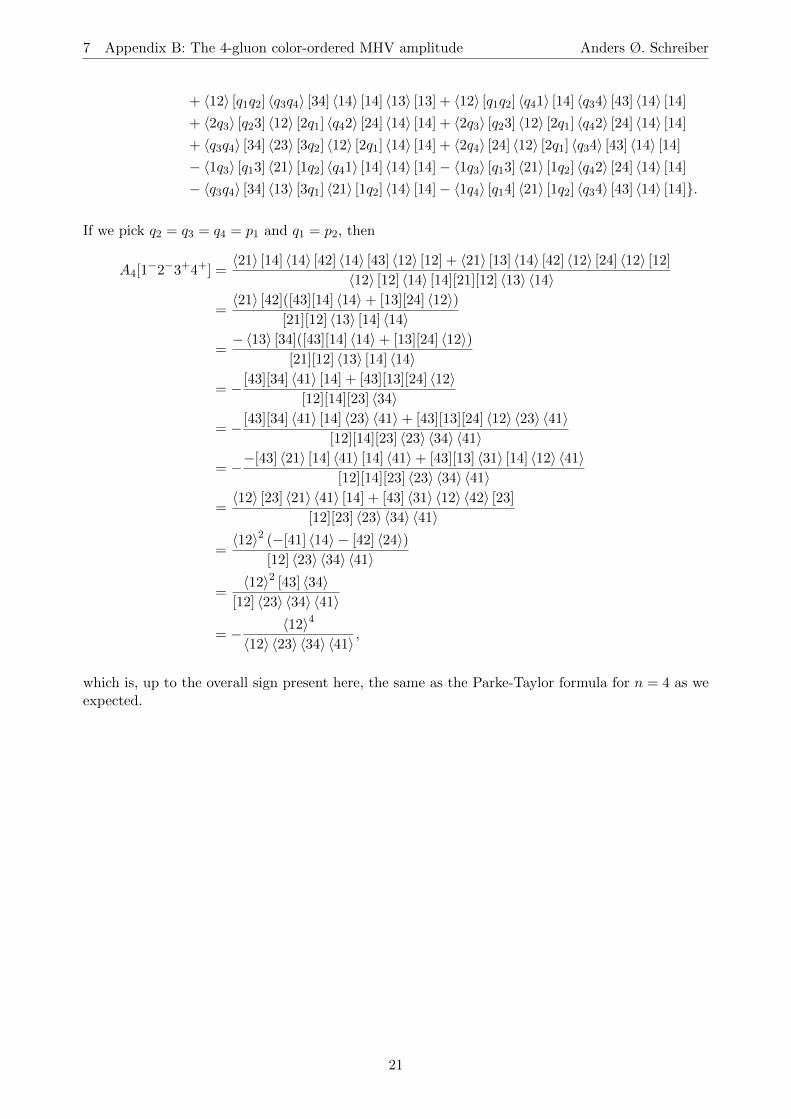
If we pick q2 = q3 = q4 = p1 and q1 = p2, then

A4[1−2−3+4+] =

〈21〉 [14] 〈14〉 [42] 〈14〉 [43] 〈12〉 [12] + 〈21〉 [13] 〈14〉 [42] 〈12〉 [24] 〈12〉 [12]

〈12〉 [12] 〈14〉 [14][21][12] 〈13〉〈14〉

=〈21〉 [42]([43][14] 〈14〉+ [13][24] 〈12〉)

[21][12] 〈13〉 [14] 〈14〉

=−〈13〉 [34]([43][14] 〈14〉+ [13][24] 〈12〉)

[21][12] 〈13〉 [14] 〈14〉

= − [43][34] 〈41〉 [14] + [43][13][24] 〈12〉[12][14][23] 〈34〉

= − [43][34] 〈41〉 [14] 〈23〉〈41〉+ [43][13][24] 〈12〉〈23〉〈41〉[12][14][23] 〈23〉〈34〉〈41〉

= −−[43] 〈21〉 [14] 〈41〉 [14] 〈41〉+ [43][13] 〈31〉 [14] 〈12〉〈41〉[12][14][23] 〈23〉〈34〉〈41〉

=〈12〉 [23] 〈21〉〈41〉 [14] + [43] 〈31〉〈12〉〈42〉 [23]

[12][23] 〈23〉〈34〉〈41〉

=〈12〉2 (−[41] 〈14〉 − [42] 〈24〉)

[12] 〈23〉〈34〉〈41〉

=〈12〉2 [43] 〈34〉

[12] 〈23〉〈34〉〈41〉

= − 〈12〉4〈12〉〈23〉〈34〉〈41〉 ,

which is, up to the overall sign present here, the same as the Parke-Taylor formula for n = 4 as weexpected.

21

8 Appendix C: Little group scaling and 3-particle amplitudes Anders Ø. Schreiber

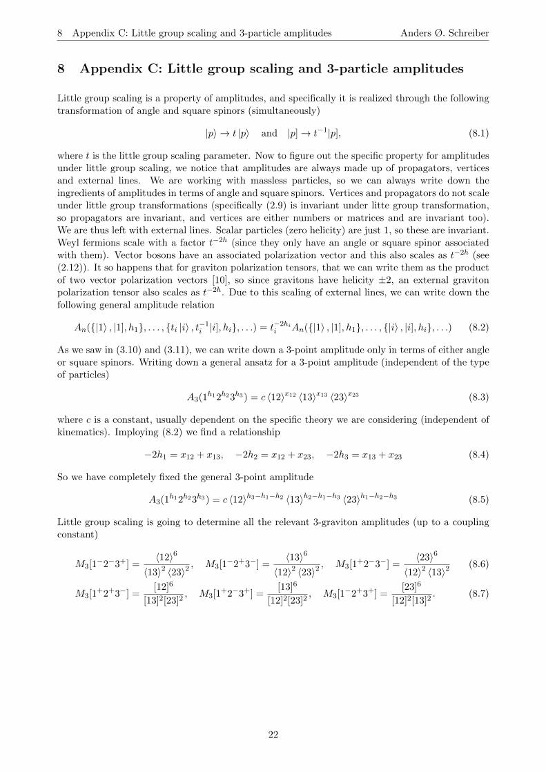
8 Appendix C: Little group scaling and 3-particle amplitudes

Little group scaling is a property of amplitudes, and specifically it is realized through the followingtransformation of angle and square spinors (simultaneously)

|p〉 → t |p〉 and |p]→ t−1|p], (8.1)

where t is the little group scaling parameter. Now to figure out the specific property for amplitudesunder little group scaling, we notice that amplitudes are always made up of propagators, verticesand external lines. We are working with massless particles, so we can always write down theingredients of amplitudes in terms of angle and square spinors. Vertices and propagators do not scaleunder little group transformations (specifically (2.9) is invariant under litte group transformation,so propagators are invariant, and vertices are either numbers or matrices and are invariant too).We are thus left with external lines. Scalar particles (zero helicity) are just 1, so these are invariant.Weyl fermions scale with a factor t−2h (since they only have an angle or square spinor associatedwith them). Vector bosons have an associated polarization vector and this also scales as t−2h (see(2.12)). It so happens that for graviton polarization tensors, that we can write them as the productof two vector polarization vectors [10], so since gravitons have helicity ±2, an external gravitonpolarization tensor also scales as t−2h. Due to this scaling of external lines, we can write down thefollowing general amplitude relation

An({|1〉 , |1], h1}, . . . , {ti |i〉 , t−1i |i], hi}, . . .) = t−2hii An({|1〉 , |1], h1}, . . . , {|i〉 , |i], hi}, . . .) (8.2)

As we saw in (3.10) and (3.11), we can write down a 3-point amplitude only in terms of either angleor square spinors. Writing down a general ansatz for a 3-point amplitude (independent of the typeof particles)

A3(1h12h23h3) = c 〈12〉x12 〈13〉x13 〈23〉x23 (8.3)

where c is a constant, usually dependent on the specific theory we are considering (independent ofkinematics). Imploying (8.2) we find a relationship

−2h1 = x12 + x13, −2h2 = x12 + x23, −2h3 = x13 + x23 (8.4)

So we have completely fixed the general 3-point amplitude

A3(1h12h23h3) = c 〈12〉h3−h1−h2 〈13〉h2−h1−h3 〈23〉h1−h2−h3 (8.5)

Little group scaling is going to determine all the relevant 3-graviton amplitudes (up to a couplingconstant)

M3[1−2−3+] =

〈12〉6

〈13〉2 〈23〉2, M3[1

−2+3−] =〈13〉6

〈12〉2 〈23〉2, M3[1

+2−3−] =〈23〉6

〈12〉2 〈13〉2(8.6)

M3[1+2+3−] =

[12]6

[13]2[23]2, M3[1

+2−3+] =[13]6

[12]2[23]2, M3[1

−2+3+] =[23]6

[12]2[13]2. (8.7)

22

References Anders Ø. Schreiber

References

[1] M. Srednicki, Quantum Field Theory, Cambridge University Press, 2007.

[2] N. Emil J. Bjerrum-Bohr, Quantum Gravity, Effective Fields and String Theory, PhD Thesis(2004).

[3] N. E. J. Bjerrum-Bohr, J. F. Donoghue, B. R. Holstein, L. Plante, and P. Vanhove, Bending ofLight in Quantum Gravity, Phys. Rev. Lett. 114, 061301 (2015).

[4] N. Arkani-Hamed, J. L. Bourjaily, F. Cachazo, A. B. Goncharov, A. Postnikov, J. Trnka, Scat-tering Amplitudes and the Positive Grassmanian, arXiv:1212.5605 [hep-th].

[5] H. Elvang and Y. Huang, Scattering Amplitudes in Gauge Theory and Gravity, First Edition,Cambridge University Press 2015.

[6] L. Dixon, Calculating Scattering Amplitudes Efficiently, arXiv:hep-ph/9601359.

[7] M. Mangano, S. Parke and Z. Xu, Duality and Multi-Gluon Scattering, Nucl. Phys. B298: 653(1988).

[8] S. J. Parke and T. R. Taylor Amplitude for n-Gluon Scattering, Phys. Rev. Lett. 56, 2459 (1986).

[9] H. Kawai, D.C. Lewellen and S.-H.H. Tye, A relation between tree amplitudes of closed and openstrings, Nucl. Phys. B269: 1 (1986).

[10] P. Benincasa, C. Boucher-Veronneau and F. Cachazo, Taming tree amplitudes in general rela-tivity, JHEP 11, 057 (2007).

[11] N. Arkani-Hamed and J. Kaplan, On tree amplitudes in gauge theory and gravity, JHEP 04,076 (2008).

[12] T. Søndergaard, Perturbative Gravity and Gauge-Theory Relations, PhD Thesis (2012).

[13] S. Sannan, Gravity as the limit of the type-II superstring theory, Phys. Rev. D, 34 6 (1986).

[14] K. Risager, A direct proof of the CSW rules, JHEP 0512, 003 (2005).

[15] H. Elvang, D. Z. Freedman, and M. Kiermaier, Proof of the MHV vertex expansion for all treeamplitudes in N = 4 SYM theory, JHEP 0906, 068 (2009).

[16] F. Cachazo, P. Svrcek and E. Witten, MHV vertices and tree amplitudes in gauge theory, JHEP0409, 006 (2004).

[17] L. J. Dixon, E. W. N. Glover, and V. V. Khoze, MHV rules for Higgs plus multi-gluon ampli-tudes, JHEP 0412, 015 (2004).

[18] S. D. Badger, E. W. N. Glover, and V. V. Khoze, MHV rules for Higgs plus multi-partonamplitudes, JHEP 0503, 023 (2005).

23

Documents

ProjectAndersSchreiber