Projecting Global Growth - Trusted Insights for Business ... · PDF fileProjecting Global Growth by Vivian Chen, ... mature and 22 emerging market economies for 2013, ... The trend

1

Projecting Global Growth

by Vivian Chen, Ben Cheng, Gad Levanon, Ataman Ozyildirim and Bart van Ark

This version: November 2012

The Conference Board, Economics Working Papers, EPWP #12 – 02

Abstract

This paper presents the methodology for The Conference Board Global Economic

Outlook 2013, including projections for 11 major regions and individual estimates for 33

mature and 22 emerging market economies for 2013, 2014—2018, and 2019–2025. The

projections are based on a supply-side based growth accounting model that estimates the

contributions of the use of labor, capital, and productivity to the growth of GDP. Capital

and productivity growth are estimated on the basis of a wide range of related variables

during past periods. The trend growth rates that are obtained from this exercise are

adjusted for possible deviations between actual and potential output.

2

1. Introduction and Summary

Since 2008, The Conference Board publishes an annual global economic outlook, projecting

GDP growth for 55 countries using growth accounting techniques. The basis of the framework is

formed by the work of Dale Jorgenson and colleagues, including Jorgenson, Ho and Stiroh (2005)

and Jorgenson and Vu (2008). Over the years we have aimed to improve the projection methods,

using more information from historical performance and adopting procedures to adjust for

cyclical deviations from trend in short term.

This paper describes the methodology and sources underlying the projections of growth of Gross

Domestic Product in the 2013 edition of The Conference Board Global Economic Outlook. It is

an expanded version of the methods implemented in the 2012 edition of the outlook, especially

by basing the methodology more strongly on variables that have an established economic

significance for the projected variables.1

The projections in this paper cover the period 2013-2025, with separate projections for the

medium term (2013-2018) and for the long term (2019-2025). The outlook covers 55 major

economies across 11 global regions, including 33 advanced economies (the United States,

Europe, Japan and other advanced economies) and 22 emerging and developing economies.

Section 2 describes how trend growth is estimated on the basis of an extrapolated growth

accounting model which projects the various growth components of the production function. For

labor quantity (Section 2.1), the measures are primarily based on projections for the working age

population (age of 15-64) from the International Data Base of the U.S. Census Bureau. For labor

composition (Section 2.2), estimates are based on projections of population by level of education

attainment, age and sex by KC et al. (2010). For capital services and total factor productivity

(Section 2.3), we use regression models which are largely based on relevant past-period variables.

The extrapolated growth accounting estimates are provided for 33 advanced economies and 22

major emerging and developing economies. Projections of all input factors are combined to

provide projections of GDP growth in Section 2.4.

1 Vivian Chen, Ben Cheng, Gad Levanon, and Bart van Ark, “Projecting Economic Growth with Growth

Accounting Techniques: The Conference Board Global Economic Outlook 2012 Sources and Methods,” The

Conference Board Economics Program Working Paper Series, EPWP #11 – 07, November 2011.

http://www.census.gov/population/international/data/idb/informationGateway.php

http://www.demographic-research.org/volumes/vol22/15/22-15.pdf

3

The projected GDP growth rates based on the growth accounting framework are to be considered

to represent the trend growth of each economy. In the long run, countries grow according to their

trend.2 In the short run, however, countries deviate from their long-run path due to temporary

fluctuations primarily due to business cycle dynamics. Occasionally, shocks can also occur

which have a deep impact on the structure of the economy, which can permanently change the

course of the trend. The 2008/09 recession represents a combination of business cycle dynamics

and shock effects, which has led to such changes. Section 3 describes the medium-term

adjustments to the trend growth estimates obtained from the extrapolated growth accounts.

Section 4 compares our GDP growth projections with those from other studies. Section 5

concludes.

The outlook for 2013 and beyond suggests some effects of a modest recovery in advanced

economies, which brings these countries to an average growth of 1.8 percent between 2013 and

2018. Among the larger economies, the United States will be outperforming Europe in 2013-

2018 by more than a full percentage point (2.3 and 1.2 percent annual GDP growth, respectively).

However, there remain significant downside risks to even this modest recovery, which could

slow growth to 1.4 percent for advanced economies as a whole.

While growth in emerging and developing economies was surprisingly strong in 2010 and 2011

(7.5 percent and 6.0 percent, respectively), such extraordinary growth started to wind down in

2012 (5.5 percent). Given the current sober conditions in the global economy, there is little scope

for emerging economies to improve their performance in the next few years. For example, the

economies of China and India begin to show signs of maturing beyond 2012, as their trend

growth will begin to slow from 2013-2018 to 2019-2025 (from 5.5 to 3.7 percent in China and

4.7 to 3.9 percent in India). Overall, emerging economies’ growth will slow to 3.3 percent on

average from 4.2 percent from 2013-2018 to 2019-2025.

2 Our trend growth rates may be seen as a proxy to the growth rate of potential output, but as our estimates do not

explicitly account for a non-inflationary constraint on our growth measure, and our estimates are not accompanied

by a measure of potential output, we prefer the use of the term “trend growth”, as our estimates are essentially

derived from past growth trends.

4

In sum, even though growth in the advanced economies is expected to recover beyond 2013,

there will be major offsetting effects from continued slower growth in the emerging markets.

Based on current trends, global GDP is projected to grow at 3.0 percent from 2013-2018, and

then show a further slowdown to 2.5 percent from 2019-2025. At 2.8 percent, on average, global

growth will still be somewhat higher than the period 1980-1995, but about a full percentage point

below the growth rate from 1996-2008.3

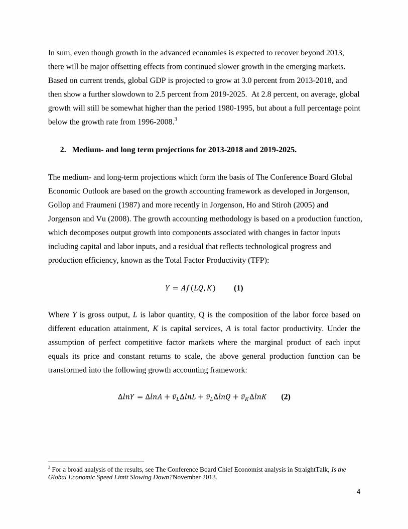
2. Medium- and long term projections for 2013-2018 and 2019-2025.

The medium- and long-term projections which form the basis of The Conference Board Global

Economic Outlook are based on the growth accounting framework as developed in Jorgenson,

Gollop and Fraumeni (1987) and more recently in Jorgenson, Ho and Stiroh (2005) and

Jorgenson and Vu (2008). The growth accounting methodology is based on a production function,

which decomposes output growth into components associated with changes in factor inputs

including capital and labor inputs, and a residual that reflects technological progress and

production efficiency, known as the Total Factor Productivity (TFP):

(1)

Where Y is gross output, L is labor quantity, Q is the composition of the labor force based on

different education attainment, K is capital services, A is total factor productivity. Under the

assumption of perfect competitive factor markets where the marginal product of each input

equals its price and constant returns to scale, the above general production function can be

transformed into the following growth accounting framework:

(2)

3 For a broad analysis of the results, see The Conference Board Chief Economist analysis in StraightTalk, Is the

Global Economic Speed Limit Slowing Down?November 2013.

5

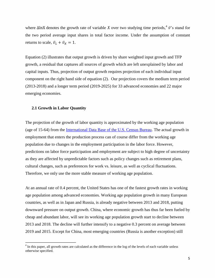
where denotes the growth rate of variable X over two studying time periods,4 ’s stand for

the two period average input shares in total factor income. Under the assumption of constant

returns to scale, .

Equation (2) illustrates that output growth is driven by share weighted input growth and TFP

growth, a residual that captures all sources of growth which are left unexplained by labor and

capital inputs. Thus, projection of output growth requires projection of each individual input

component on the right hand side of equation (2). Our projection covers the medium term period

(2013-2018) and a longer term period (2019-2025) for 33 advanced economies and 22 major

emerging economies.

2.1 Growth in Labor Quantity

The projection of the growth of labor quantity is approximated by the working age population

(age of 15-64) from the International Data Base of the U.S. Census Bureau. The actual growth in

employment that enters the production process can of course differ from the working age

population due to changes in the employment participation in the labor force. However,

predictions on labor force participation and employment are subject to high degree of uncertainty

as they are affected by unpredictable factors such as policy changes such as retirement plans,

cultural changes, such as preferences for work vs. leisure, as well as cyclical fluctuations.

Therefore, we only use the more stable measure of working age population.

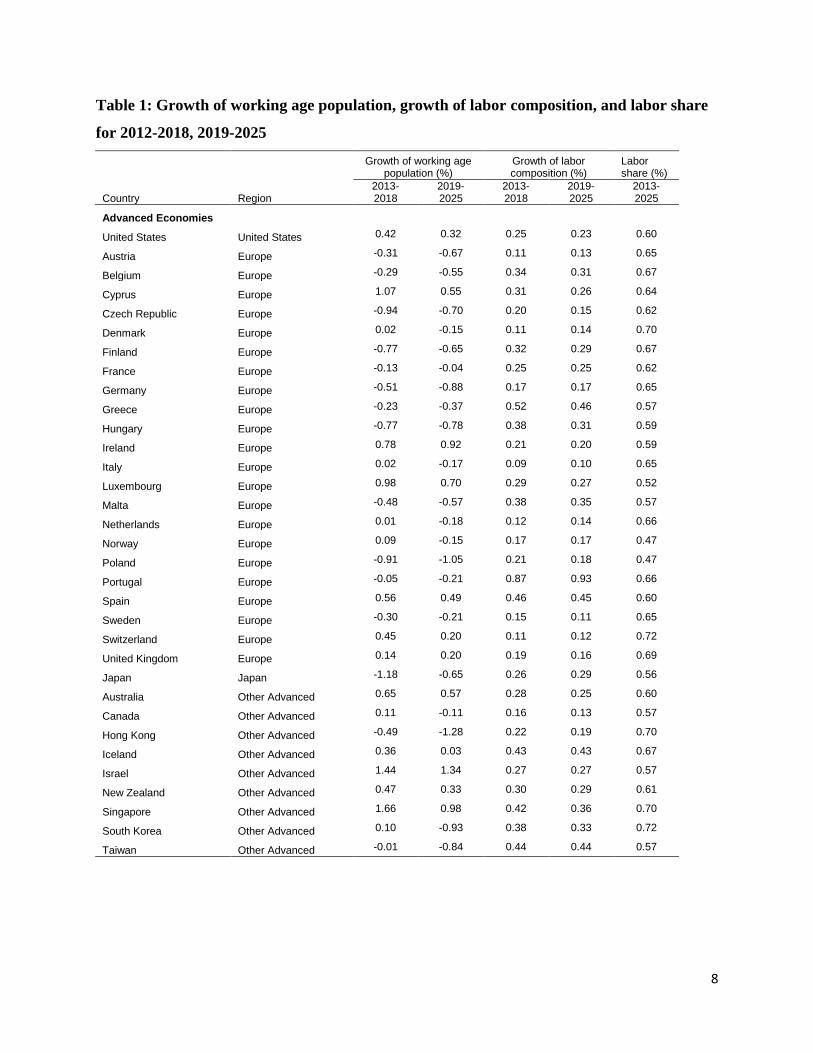
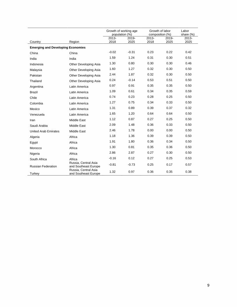
At an annual rate of 0.4 percent, the United States has one of the fastest growth rates in working

age population among advanced economies. Working age population growth in many European

countries, as well as in Japan and Russia, is already negative between 2013 and 2018, putting

downward pressure on output growth. China, where economic growth has thus far been fueled by

cheap and abundant labor, will see its working age population growth start to decline between

2013 and 2018. The decline will further intensify to a negative 0.3 percent on average between

2019 and 2015. Except for China, most emerging countries (Russia is another exception) still

4 In this paper, all growth rates are calculated as the difference in the log of the levels of each variable unless

otherwise specified.


6

enjoy the demographic dividend as their working age population continues to grow though the

pace of the growth will slow from 2013-2018 period to 2019-2025 period.

2.2 Growth in Labor Composition

In addition to the change in labor quantity, an adjustment for changes in the composition of the

labor force in terms of different skill-levels is needed to measure labor’s effective contribution to

output growth. The change of labor composition is constructed on the basis of weighted

measures of different skill-level groups (low, medium and high skilled workers based on

educational attainment) in the labor force:

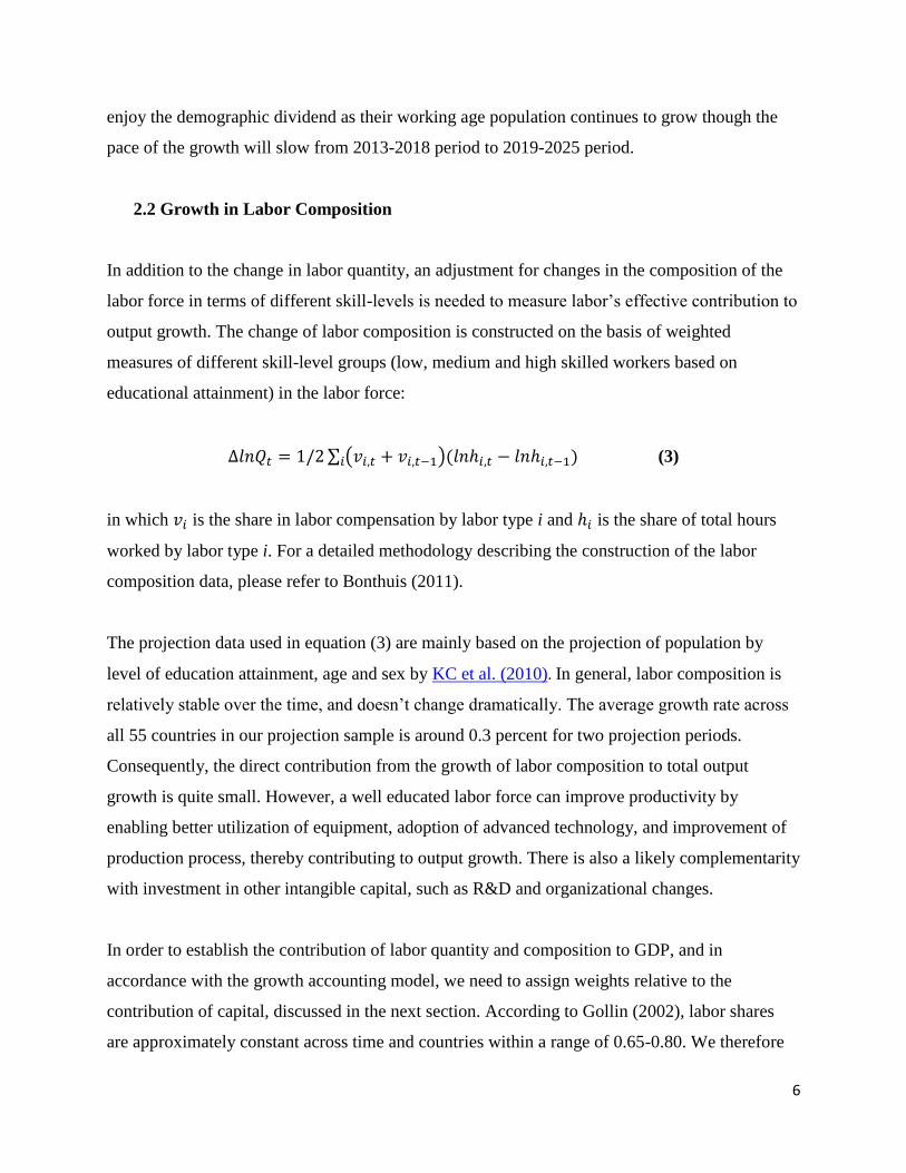
∑ ( ) (3)

in which is the share in labor compensation by labor type i and is the share of total hours

worked by labor type i. For a detailed methodology describing the construction of the labor

composition data, please refer to Bonthuis (2011).

The projection data used in equation (3) are mainly based on the projection of population by

level of education attainment, age and sex by KC et al. (2010). In general, labor composition is

relatively stable over the time, and doesn’t change dramatically. The average growth rate across

all 55 countries in our projection sample is around 0.3 percent for two projection periods.

Consequently, the direct contribution from the growth of labor composition to total output

growth is quite small. However, a well educated labor force can improve productivity by

enabling better utilization of equipment, adoption of advanced technology, and improvement of

production process, thereby contributing to output growth. There is also a likely complementarity

with investment in other intangible capital, such as R&D and organizational changes.

In order to establish the contribution of labor quantity and composition to GDP, and in

accordance with the growth accounting model, we need to assign weights relative to the

contribution of capital, discussed in the next section. According to Gollin (2002), labor shares

are approximately constant across time and countries within a range of 0.65-0.80. We therefore

http://www.demographic-research.org/volumes/vol22/15/22-15.pdf

7

use the average labor share for individual countries in 2006-2012 for the projection years. On

average labor shares are lower in emerging economies because capital is scarcer while labor is

cheaper compared to advanced economies. Our data (see Table 1) confirm this pattern: Mexico,

Turkey and China, have the lowest labor share (between 0.32-0.42) among our projection

countries while labor shares in Korea and Switzerland are more than 0.7.5

5 For countries that we do not have labor share data for, we use 0.7 for advanced countries and 0.5 for emerging

economies.

8

Table 1: Growth of working age population, growth of labor composition, and labor share

for 2012-2018, 2019-2025

Growth of working age

population (%) Growth of labor composition (%)

Labor share (%)

Country Region 2013-2018

2019-2025

2013-2018

2019-2025

2013-2025

Advanced Economies

United States United States 0.42 0.32 0.25 0.23 0.60

Austria Europe -0.31 -0.67 0.11 0.13 0.65

Belgium Europe -0.29 -0.55 0.34 0.31 0.67

Cyprus Europe 1.07 0.55 0.31 0.26 0.64

Czech Republic Europe -0.94 -0.70 0.20 0.15 0.62

Denmark Europe 0.02 -0.15 0.11 0.14 0.70

Finland Europe -0.77 -0.65 0.32 0.29 0.67

France Europe -0.13 -0.04 0.25 0.25 0.62

Germany Europe -0.51 -0.88 0.17 0.17 0.65

Greece Europe -0.23 -0.37 0.52 0.46 0.57

Hungary Europe -0.77 -0.78 0.38 0.31 0.59

Ireland Europe 0.78 0.92 0.21 0.20 0.59

Italy Europe 0.02 -0.17 0.09 0.10 0.65

Luxembourg Europe 0.98 0.70 0.29 0.27 0.52

Malta Europe -0.48 -0.57 0.38 0.35 0.57

Netherlands Europe 0.01 -0.18 0.12 0.14 0.66

Norway Europe 0.09 -0.15 0.17 0.17 0.47

Poland Europe -0.91 -1.05 0.21 0.18 0.47

Portugal Europe -0.05 -0.21 0.87 0.93 0.66

Spain Europe 0.56 0.49 0.46 0.45 0.60

Sweden Europe -0.30 -0.21 0.15 0.11 0.65

Switzerland Europe 0.45 0.20 0.11 0.12 0.72

United Kingdom Europe 0.14 0.20 0.19 0.16 0.69

Japan Japan -1.18 -0.65 0.26 0.29 0.56

Australia Other Advanced 0.65 0.57 0.28 0.25 0.60

Canada Other Advanced 0.11 -0.11 0.16 0.13 0.57

Hong Kong Other Advanced -0.49 -1.28 0.22 0.19 0.70

Iceland Other Advanced 0.36 0.03 0.43 0.43 0.67

Israel Other Advanced 1.44 1.34 0.27 0.27 0.57

New Zealand Other Advanced 0.47 0.33 0.30 0.29 0.61

Singapore Other Advanced 1.66 0.98 0.42 0.36 0.70

South Korea Other Advanced 0.10 -0.93 0.38 0.33 0.72

Taiwan Other Advanced -0.01 -0.84 0.44 0.44 0.57

9

Growth of working age

population (%) Growth of labor composition (%)

Labor share (%)

Country Region 2013-2018

2019-2025

2013-2018

2019-2025

2013-2025

Emerging and Developing Economies

China China -0.02 -0.31 0.23 0.22 0.42

India India 1.59 1.24 0.31 0.30 0.51

Indonesia Other Developing Asia 1.30 0.80 0.30 0.30 0.46

Malaysia Other Developing Asia 1.60 1.27 0.32 0.30 0.50

Pakistan Other Developing Asia 2.44 1.87 0.32 0.30 0.50

Thailand Other Developing Asia 0.24 -0.14 0.53 0.51 0.50

Argentina Latin America 0.97 0.91 0.35 0.35 0.50

Brazil Latin America 1.09 0.61 0.34 0.35 0.59

Chile Latin America 0.74 0.23 0.28 0.25 0.50

Colombia Latin America 1.27 0.75 0.34 0.33 0.50

Mexico Latin America 1.31 0.89 0.39 0.37 0.32

Venezuela Latin America 1.65 1.20 0.64 0.64 0.50

Iran Middle East 1.12 0.87 0.27 0.25 0.50

Saudi Arabia Middle East 2.09 1.48 0.36 0.33 0.50

United Arab Emirates Middle East 2.46 1.78 0.00 0.00 0.50

Algeria Africa 1.18 1.36 0.39 0.39 0.50

Egypt Africa 1.91 1.80 0.36 0.34 0.50

Morocco Africa 1.30 0.81 0.35 0.36 0.50

Nigeria Africa 2.86 2.87 0.27 0.30 0.50

South Africa Africa -0.16 0.12 0.27 0.25 0.53

Russian Federation Russia, Central Asia and Southeast Europe

-0.81 -0.73 0.25 0.17 0.57

Turkey Russia, Central Asia and Southeast Europe

1.32 0.97 0.36 0.35 0.38

10

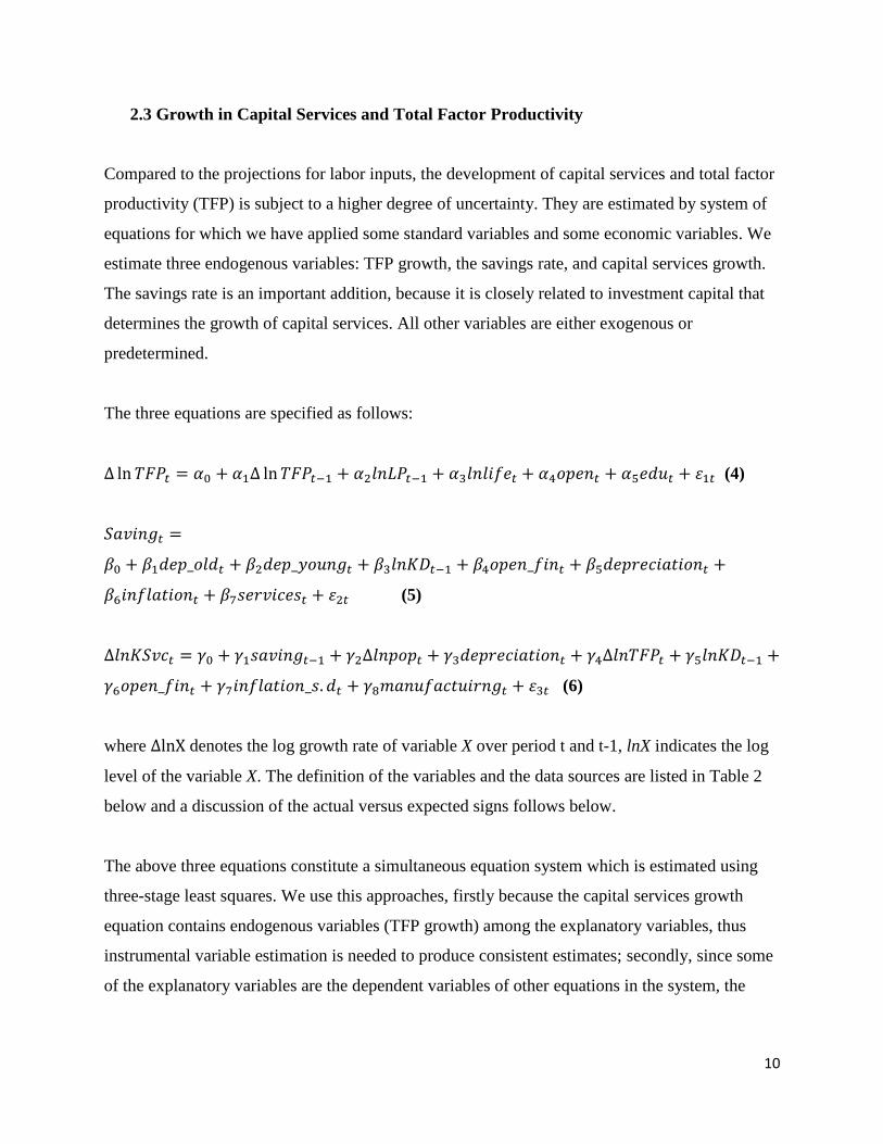
2.3 Growth in Capital Services and Total Factor Productivity

Compared to the projections for labor inputs, the development of capital services and total factor

productivity (TFP) is subject to a higher degree of uncertainty. They are estimated by system of

equations for which we have applied some standard variables and some economic variables. We

estimate three endogenous variables: TFP growth, the savings rate, and capital services growth.

The savings rate is an important addition, because it is closely related to investment capital that

determines the growth of capital services. All other variables are either exogenous or

predetermined.

The three equations are specified as follows:

(4)

(5)

(6)

where denotes the log growth rate of variable X over period t and t-1, lnX indicates the log

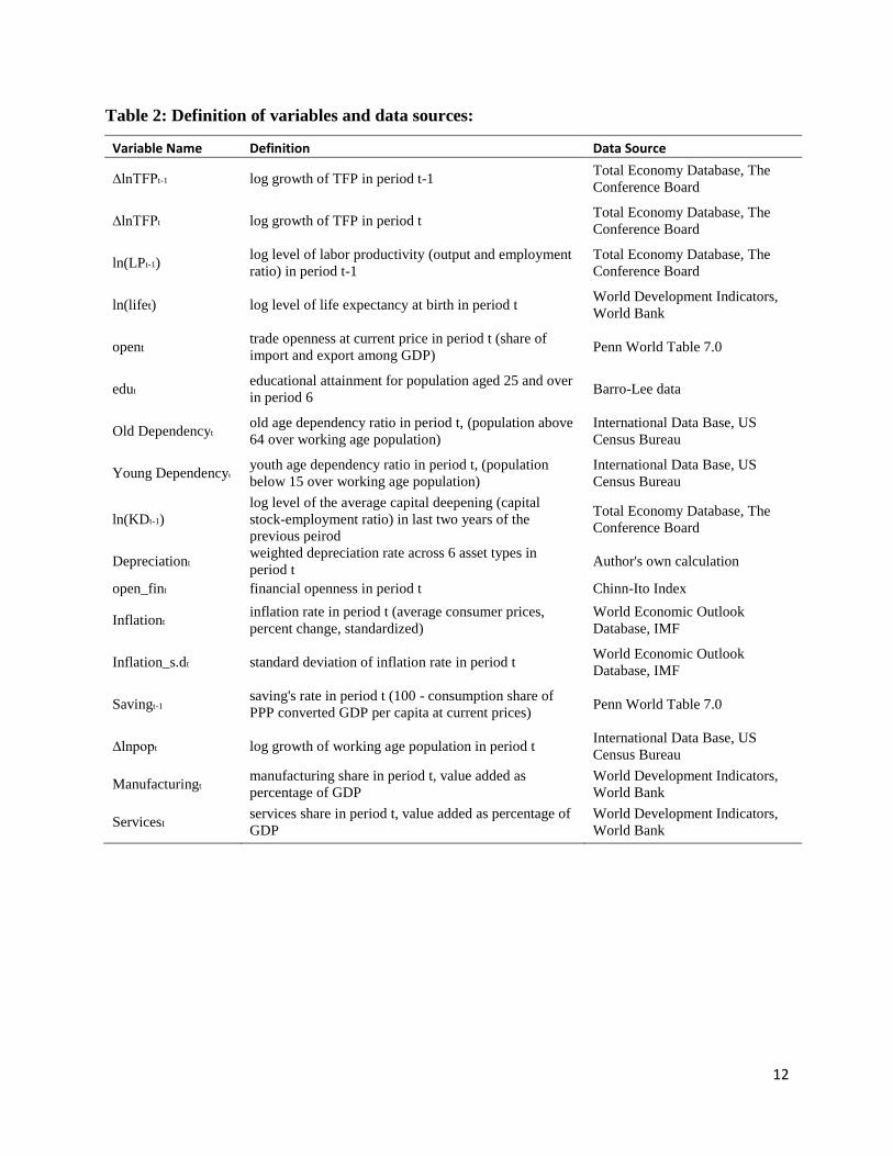
level of the variable X. The definition of the variables and the data sources are listed in Table 2

below and a discussion of the actual versus expected signs follows below.

The above three equations constitute a simultaneous equation system which is estimated using

three-stage least squares. We use this approaches, firstly because the capital services growth

equation contains endogenous variables (TFP growth) among the explanatory variables, thus

instrumental variable estimation is needed to produce consistent estimates; secondly, since some

of the explanatory variables are the dependent variables of other equations in the system, the

11

three error terms are expected to be correlated, thus generalized least squares should be used to

account for the correlation among the error terms across equations.

To implement our regressions, we restrict our sample to 33 advanced economies and 22 major

emerging economies from 1972 to 2012 to ensure the high quality of the data. We divide the 41

years into six time periods: 1972-1978, 1979-1986, 1987-1992, 1993-1998, 1999-2005, and

2006-2012. These divisions are designed to distribute the number of years to each period as

equally as possible. More importantly, we choose divisions so that the initial and end years do

not fall on recession years.6 All annual variables from the data sources are averaged for each

defined period.

6 Recession years vary across countries. We choose divisions based on U.S. recession years because the U.S. is the

largest economy.

12

Table 2: Definition of variables and data sources:

Variable Name Definition Data Source

∆lnTFPt-1 log growth of TFP in period t-1 Total Economy Database, The

Conference Board

∆lnTFPt log growth of TFP in period t Total Economy Database, The

Conference Board

ln(LPt-1) log level of labor productivity (output and employment

ratio) in period t-1

Total Economy Database, The

Conference Board

ln(lifet) log level of life expectancy at birth in period t World Development Indicators,

World Bank

opent trade openness at current price in period t (share of

import and export among GDP) Penn World Table 7.0

edut educational attainment for population aged 25 and over

in period 6 Barro-Lee data

Old Dependencyt old age dependency ratio in period t, (population above

64 over working age population)

International Data Base, US

Census Bureau

Young Dependencyt youth age dependency ratio in period t, (population

below 15 over working age population)

International Data Base, US

Census Bureau

ln(KDt-1)

log level of the average capital deepening (capital

stock-employment ratio) in last two years of the

previous peirod

Total Economy Database, The

Conference Board

Depreciationt weighted depreciation rate across 6 asset types in

period t Author's own calculation

open_fint financial openness in period t Chinn-Ito Index

Inflationt inflation rate in period t (average consumer prices,

percent change, standardized)

World Economic Outlook

Database, IMF

Inflation_s.dt standard deviation of inflation rate in period t World Economic Outlook

Database, IMF

Savingt-1 saving's rate in period t (100 - consumption share of

PPP converted GDP per capita at current prices) Penn World Table 7.0

∆lnpopt log growth of working age population in period t International Data Base, US

Census Bureau

Manufacturingt manufacturing share in period t, value added as

percentage of GDP

World Development Indicators,

World Bank

Servicest services share in period t, value added as percentage of

GDP

World Development Indicators,

World Bank

13

Table 3: Estimation results of simultaneous equations

TFP Growth

Saving

K Services Growth

∆lnTFPt-1 0.0504

(0.98)

ln(LPt-1) -1.056***

(-5.84)

ln(lifet) 2.600*

(1.77)

opent 0.00482***

(3.25)

edut 0.159***

(3.09)

Old Dependencyt

-0.842***

(-7.34)

Young Dependencyt

-0.167***

(-3.46)

ln(KDt-1)

5.086***

-1.112***

(6.90)

(-6.41)

Depreciationt

1.869***

0.425***

(3.79)

(3.23)

open_fint

1.232***

0.128

(2.83)

(1.16)

Inflationt

-0.786

(-0.97)

Servicest

-0.458***

(-7.24)

∆lnTFPt

0.367*

(1.66)

Savingt-1

0.0250

(1.57)

∆lnpopt

0.396**

(2.32)

Inflation_s.dt

-0.00246**

(-2.39)

Manufacturingt

0.0737***

(2.93)

Constant -1.522

6.255

10.81***

(-0.28)

(0.69)

(5.01)

The system of equations is estimated by the 3SLS (three-stage least squares) method.

Total number of observations: 236

z statistics in parentheses

* P<0.1; ** P<0.05; *** P<0.01

14

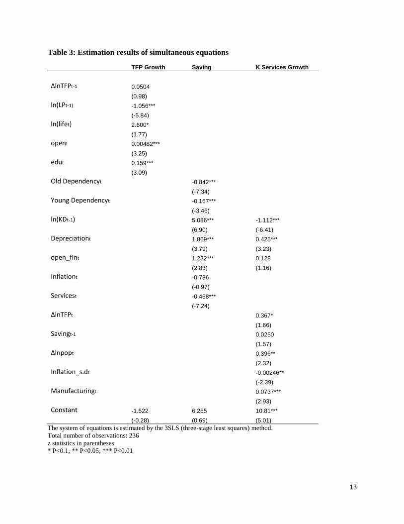
Table 3 reports the results of the simultaneous equation system using the three-stage least

squares estimation. The results are largely consistent with theoretical expectations. Specifically,

the lagged labor productivity variable in TFP growth equation and the lagged capital deepening

variable in the capital services growth equation are specified to test the convergence hypothesis.7

Both of these two lagged variables are significantly negative, lending support to the convergence

hypothesis as the country with higher labor productivity (or capital deepening) level will have

slower growth of total factor productivity (capital services) in the next period. In addition to the

convergence effect, there are some other results worth noting:

A. In the TFP growth equation, the coefficients of life expectancy, trade openness and

education level are all significantly positive. Longer life expectancy is closely related to

better health conditions, a foundation for faster productivity growth. A better educated

labor force is equipped with the necessary knowledge and skills to unravel the

productivity in the production process. Trade openness improves TFP growth probably

via the channel of specialization. 8

B. In the savings equation, both old and youth dependency ratio have a negative effect on

the savings rate as population in these age cohorts mostly do not have income and are

major consumers of education and health care. Higher inflation also affects savings

negatively as it depreciates the money saved for future use. The negative relationship

between the share of the services sector in an economy and the savings rate probably

results from the larger presence of government funded social services, education and

health care, causing people to have less precautionary savings. On the other hand,

depreciation and financial openness have significant positive effect on savings. A higher

depreciation rate requires higher investment (from savings) to maintain the current capital

stock levels. Higher financial openness encourages savings probably because once people

have access to more and better financial instruments, they are motivated to save more of

their current income to invest in various financial products to increase their wealth.

7 Ideally, we want to use TFP and capital services level of the initial year to test convergence. Since we do not have

the level data for TFP and capital services for all countries, labor productivity and capital deepening levels are used

instead in the specification. 8 Alcala and Ciccone (2003) find the causal effect of trade on productivity across countries is statistically and

economically significant as well as robust.

15

C. In the capital services growth equation, the savings rate, financial openness, population

growth, and manufacturing share all lead to higher growth in capital services as one

would expect. Intuitively, the growth accounting identity imposes a negative relationship

between TFP and capital services growth because TFP growth is calculated as a residual

in the equation. However, if TFP growth is pure exogenous, it can affect capital services

positively probably by pushing out the productivity frontier. The significant positive

relationship between capital services and TFP growth according to the simultaneous

equations show that faster TFP growth promotes growth in capital services probably via

increased efficiency in the production process. This result contracts the single equation

estimation result, in which TFP growth has a negative (though not significant) effect on

capital services growth. The difference arises because TFP growth is affected by some of

the same unobserved factors that affect capital services growth, such as institutional

factors. This endogeneity problem is taken care of in the simultaneous equation system

by the 3SLS estimation method. The positive effect from financial openness is probably

related to easier access to investment capital. The positive effect from manufacturing

sector is very significant as the manufacturing sector is the most capital intensive. The

standard deviation of inflation is used as a proxy for the stability of the macroeconomic

environment. The significant negative effect indicates that unstable macro conditions

may deter investment and consequently growth in capital services.

2.4 Growth Projections

Equations (4) – (6) are estimated using the actual data from periods 1 to 6. The estimated

coefficients are then used to derive projections for TFP and capital services growth. To project

TFP and capital services growth for both medium-term (2013-2018, period 7) and long-term

(2019-2025, period 8), we also need to know all the exogenous variables in the system, which

can be divided into three categories.

A. The first category includes variables whose values of medium- and long-term are given:

old and youth dependency ratios, as well as growth in working age population are

provided by International Data Base of the US Census Bureau.

16

B. The second category includes lagged variables whose long-term values need to be

calculated based on medium-term projection: lagged TFP growth, lagged savings rate,

lagged labor productivity and lagged capital deepening. The period 8 value of the first

two lagged variables can be obtained by the projected value of period 7. The lagged labor

productivity level in period 8 is calculated through labor productivity growth, which is

obtained from the difference between GDP growth and employment growth. GDP growth

in period 7 is obtained using projected capital services and TFP growth as explained

above. Employment growth is approximated by the growth of the working age population

available from the International Data Base of the US Census Bureau. The lagged capital

deepening in period 8 is calculated based on the projected growth of capital services in

period 7 together with the growth of working age population.

C. The third category includes contemporary variables whose period 7 and 8 values are

subject to judgment: inflation, standard deviation of inflation, manufacturing and services

share in total value added, life expectancy, trade and financial openness, education

attainment. Shares of manufacturing and services sectors reflect the structure of the

economy; inflation rate and the standard deviation of inflation characterize the macro

condition. The period 7 & 8 values of all these four variables are assumed to remain the

same as period 6. Life expectancy, trade and financial openness and education attainment

are considered as policy oriented variables, whose values are subject to change depending

on a country’s economic condition and development strategy. As a base scenario, we

assume all these four policy oriented variables to remain the same as their period 6 value

for period 7 & 8.9

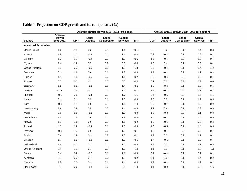
Table 4 lists GDP projections for periods 7 (2013-2018) and 8 (2019-2025) for all 55 economies

as well as the growth contributions of labor, capital and TFP. The average actual GDP growth

between 2006 and 2012 is also reported in the table for comparison purpose.10

9 As the coefficients of these four policy oriented variables are all positive, a positive deviation from the base case

will increase the projected capital services and TFP growth, and consequently GDP growth; and a negative deviation

from the base case will reduce the projected growth. 10

To evaluate the accuracy of our projection, we carried out out-of -sample tests on capital services growth, TFP

growth and GDP growth to measure the deviation of the forecast value from the actual value for period 5 (1999-

2005) and 6 (2006-2012). Please see Appendix for details.

17

Among the advanced economies, GDP growth in the U.S. and most European countries are

projected to recover between 2013 and 2018 from the period of 2006 – 2012, which includes the

great recession and the on-going European debt crisis. The recovery will be most noticeable in

those troubled European countries, such as Greece, Ireland, Italy, Portugal and Spain. On the

other hand, Poland will see a significant growth slow-down from 4.3 percent during the 2006-

2012 period to 1.9 percent during the 2013-2018 period. Outside the U.S. and Europe, most other

advanced economies will experience a decline in GDP growth during the 2013-2018 period.

Such decline will be most evident in the four Asian tigers. Japan will gain half a percentage

growth on average in the next six years. Except for the U.S. and France, the projected GDP

growth will further slow down during the 2019-2025 period in all other advanced countries.

Majority of the emerging economies in our sample experienced higher average GDP growth

during 2006-2012 than the projected GDP growth in the following period (2013-2018). China,

India and Russia ranked the top three in terms of their extraordinary performance during 2006-

2012 compared to the projected growth in 2013-2018. The high speed economic growth in

emerging countries will abate across the board after 2018 with the projected trend growth of

2019-2025 ubiquitously lower than, if not equal to, that of 2013-2018.

18

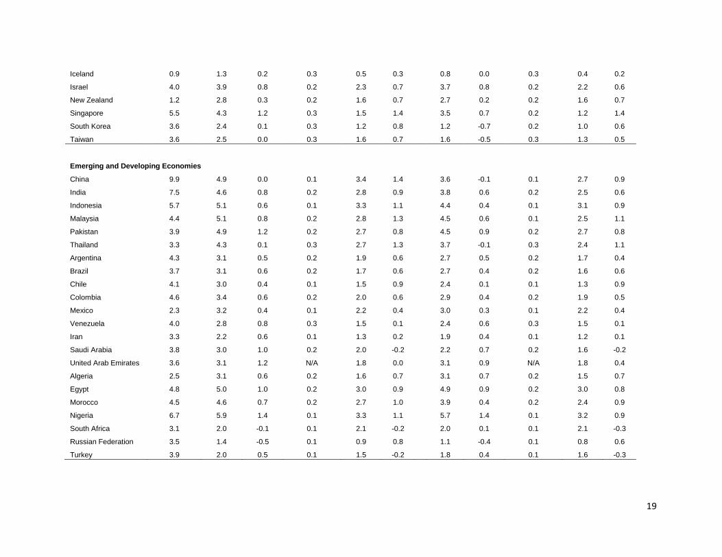
Table 4: Projection on GDP growth and its components (%)

Average annual growth 2013 - 2018 (projection) Average annual growth 2019 - 2025 (projection)

country

Average growth

2006-2012 GDP Labor

Quantity Labor

Composition Capital

Services TFP GDP Labor

Quantity Labor

Composition Capital

Services TFP

Advanced Economies

United States 1.0 1.9 0.3 0.1 1.4 0.1

2.0 0.2 0.1 1.4 0.3

Austria 1.5 1.1 -0.2 0.1 1.1 0.2

0.7 -0.4 0.1 0.9 0.1

Belgium 1.2 1.7 -0.2 0.2 1.2 0.5

1.3 -0.4 0.2 1.0 0.4

Cyprus 1.4 1.9 0.7 0.2 0.6 0.4

1.5 0.4 0.2 0.6 0.4

Czech Republic 2.1 2.3 -0.6 0.1 1.5 1.3

2.3 -0.4 0.1 1.4 1.2

Denmark 0.1 1.6 0.0 0.1 1.2 0.3

1.4 -0.1 0.1 1.1 0.3

Finland 1.1 1.0 -0.5 0.2 1.1 0.2

0.8 -0.4 0.2 0.9 0.1

France 0.7 0.2 -0.1 0.2 0.2 0.0

0.3 0.0 0.2 0.2 0.0

Germany 1.5 1.8 -0.3 0.1 1.4 0.6

1.2 -0.6 0.1 1.2 0.5

Greece -1.6 1.6 -0.1 0.3 1.3 0.1

1.4 -0.2 0.3 1.2 0.2

Hungary -0.1 2.5 -0.4 0.2 1.7 1.1

2.4 -0.5 0.2 1.6 1.1

Ireland 0.1 3.1 0.5 0.1 2.0 0.6

3.0 0.5 0.1 1.9 0.5

Italy -0.4 1.1 0.0 0.1 1.1 -0.1

0.9 -0.1 0.1 1.0 0.0

Luxembourg 1.6 2.9 0.5 0.2 1.4 0.8

2.3 0.4 0.1 0.9 0.9

Malta 2.1 2.0 -0.3 0.2 1.2 0.9

1.8 -0.3 0.2 1.1 0.8

Netherlands 1.0 1.8 0.0 0.1 1.2 0.6

1.5 -0.1 0.1 1.0 0.5

Norway 1.1 1.5 0.0 0.1 1.1 0.2

1.2 -0.1 0.1 0.9 0.3

Poland 4.3 1.9 -0.4 0.1 1.6 0.6

1.5 -0.5 0.1 1.4 0.5

Portugal -0.4 1.7 0.0 0.6 1.0 0.1

1.5 -0.1 0.6 0.9 0.1

Spain 0.4 1.9 0.3 0.3 1.2 0.1

1.7 0.3 0.3 1.1 0.1

Sweden 1.7 1.9 -0.2 0.1 1.5 0.5

1.7 -0.1 0.1 1.3 0.4

Switzerland 1.9 2.1 0.3 0.1 1.3 0.4

1.7 0.1 0.1 1.1 0.3

United Kingdom 0.4 1.1 0.1 0.1 1.0 -0.1

1.1 0.1 0.1 1.0 -0.1

Japan 0.4 0.9 -0.7 0.1 1.1 0.3

0.9 -0.4 0.2 0.9 0.2

Australia 2.7 2.2 0.4 0.2 1.5 0.2

2.1 0.3 0.1 1.4 0.2

Canada 1.5 2.0 0.1 0.1 1.4 0.4

1.7 -0.1 0.1 1.3 0.4

Hong Kong 3.7 2.2 -0.3 0.2 0.6 1.8

1.1 -0.9 0.1 0.3 1.6

19

Iceland 0.9 1.3 0.2 0.3 0.5 0.3

0.8 0.0 0.3 0.4 0.2

Israel 4.0 3.9 0.8 0.2 2.3 0.7

3.7 0.8 0.2 2.2 0.6

New Zealand 1.2 2.8 0.3 0.2 1.6 0.7

2.7 0.2 0.2 1.6 0.7

Singapore 5.5 4.3 1.2 0.3 1.5 1.4

3.5 0.7 0.2 1.2 1.4

South Korea 3.6 2.4 0.1 0.3 1.2 0.8

1.2 -0.7 0.2 1.0 0.6

Taiwan 3.6 2.5 0.0 0.3 1.6 0.7 1.6 -0.5 0.3 1.3 0.5


China 9.9 4.9 0.0 0.1 3.4 1.4

3.6 -0.1 0.1 2.7 0.9

India 7.5 4.6 0.8 0.2 2.8 0.9

3.8 0.6 0.2 2.5 0.6

Indonesia 5.7 5.1 0.6 0.1 3.3 1.1

4.4 0.4 0.1 3.1 0.9

Malaysia 4.4 5.1 0.8 0.2 2.8 1.3

4.5 0.6 0.1 2.5 1.1

Pakistan 3.9 4.9 1.2 0.2 2.7 0.8

4.5 0.9 0.2 2.7 0.8

Thailand 3.3 4.3 0.1 0.3 2.7 1.3

3.7 -0.1 0.3 2.4 1.1

Argentina 4.3 3.1 0.5 0.2 1.9 0.6

2.7 0.5 0.2 1.7 0.4

Brazil 3.7 3.1 0.6 0.2 1.7 0.6

2.7 0.4 0.2 1.6 0.6

Chile 4.1 3.0 0.4 0.1 1.5 0.9

2.4 0.1 0.1 1.3 0.9

Colombia 4.6 3.4 0.6 0.2 2.0 0.6

2.9 0.4 0.2 1.9 0.5

Mexico 2.3 3.2 0.4 0.1 2.2 0.4

3.0 0.3 0.1 2.2 0.4

Venezuela 4.0 2.8 0.8 0.3 1.5 0.1

2.4 0.6 0.3 1.5 0.1

Iran 3.3 2.2 0.6 0.1 1.3 0.2

1.9 0.4 0.1 1.2 0.1

Saudi Arabia 3.8 3.0 1.0 0.2 2.0 -0.2

2.2 0.7 0.2 1.6 -0.2

United Arab Emirates 3.6 3.1 1.2 N/A 1.8 0.0

3.1 0.9 N/A 1.8 0.4

Algeria 2.5 3.1 0.6 0.2 1.6 0.7

3.1 0.7 0.2 1.5 0.7

Egypt 4.8 5.0 1.0 0.2 3.0 0.9

4.9 0.9 0.2 3.0 0.8

Morocco 4.5 4.6 0.7 0.2 2.7 1.0

3.9 0.4 0.2 2.4 0.9

Nigeria 6.7 5.9 1.4 0.1 3.3 1.1

5.7 1.4 0.1 3.2 0.9

South Africa 3.1 2.0 -0.1 0.1 2.1 -0.2

2.0 0.1 0.1 2.1 -0.3

Russian Federation 3.5 1.4 -0.5 0.1 0.9 0.8

1.1 -0.4 0.1 0.8 0.6

Turkey 3.9 2.0 0.5 0.1 1.5 -0.2 1.8 0.4 0.1 1.6 -0.3

20

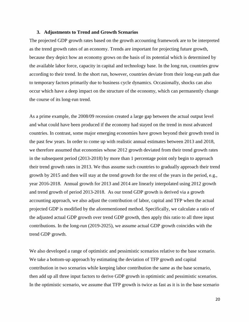
3. Adjustments to Trend and Growth Scenarios

The projected GDP growth rates based on the growth accounting framework are to be interpreted

as the trend growth rates of an economy. Trends are important for projecting future growth,

because they depict how an economy grows on the basis of its potential which is determined by

the available labor force, capacity in capital and technology base. In the long run, countries grow

according to their trend. In the short run, however, countries deviate from their long-run path due

to temporary factors primarily due to business cycle dynamics. Occasionally, shocks can also

occur which have a deep impact on the structure of the economy, which can permanently change

the course of its long-run trend.

As a prime example, the 2008/09 recession created a large gap between the actual output level

and what could have been produced if the economy had stayed on the trend in most advanced

countries. In contrast, some major emerging economies have grown beyond their growth trend in

the past few years. In order to come up with realistic annual estimates between 2013 and 2018,

we therefore assumed that economies whose 2012 growth deviated from their trend growth rates

in the subsequent period (2013-2018) by more than 1 percentage point only begin to approach

their trend growth rates in 2013. We thus assume such countries to gradually approach their trend

growth by 2015 and then will stay at the trend growth for the rest of the years in the period, e.g.,

year 2016-2018. Annual growth for 2013 and 2014 are linearly interpolated using 2012 growth

and trend growth of period 2013-2018. As our trend GDP growth is derived via a growth

accounting approach, we also adjust the contribution of labor, capital and TFP when the actual

projected GDP is modified by the aforementioned method. Specifically, we calculate a ratio of

the adjusted actual GDP growth over trend GDP growth, then apply this ratio to all three input

contributions. In the long-run (2019-2025), we assume actual GDP growth coincides with the

trend GDP growth.

We also developed a range of optimistic and pessimistic scenarios relative to the base scenario.

We take a bottom-up approach by estimating the deviation of TFP growth and capital

contribution in two scenarios while keeping labor contribution the same as the base scenario,

then add up all three input factors to derive GDP growth in optimistic and pessimistic scenarios.

In the optimistic scenario, we assume that TFP growth is twice as fast as it is in the base scenario

21

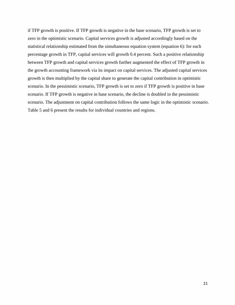
if TFP growth is positive. If TFP growth is negative in the base scenario, TFP growth is set to

zero in the optimistic scenario. Capital services growth is adjusted accordingly based on the

statistical relationship estimated from the simultaneous equation system (equation 6): for each

percentage growth in TFP, capital services will growth 0.4 percent. Such a positive relationship

between TFP growth and capital services growth further augmented the effect of TFP growth in

the growth accounting framework via its impact on capital services. The adjusted capital services

growth is then multiplied by the capital share to generate the capital contribution in optimistic

scenario. In the pessimistic scenario, TFP growth is set to zero if TFP growth is positive in base

scenario. If TFP growth is negative in base scenario, the decline is doubled in the pessimistic

scenario. The adjustment on capital contribution follows the same logic in the optimistic scenario.

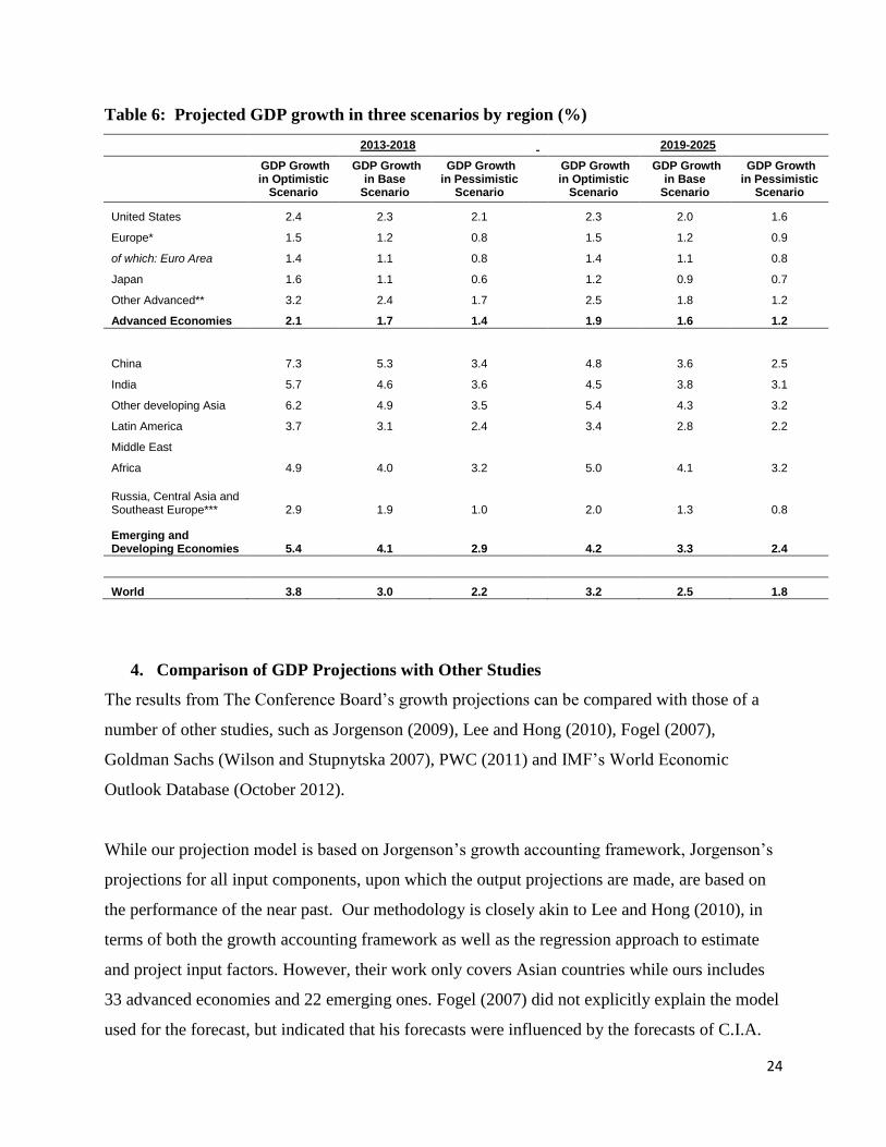
Table 5 and 6 present the results for individual countries and regions.

22

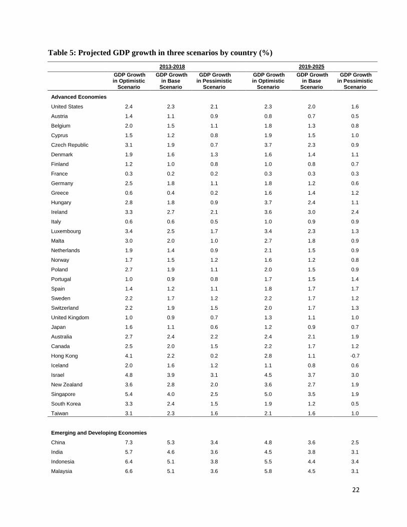
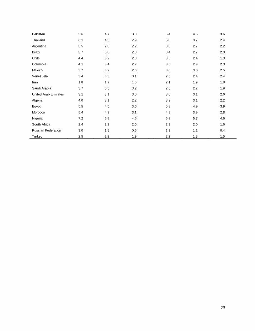
Table 5: Projected GDP growth in three scenarios by country (%)

2013-2018

2019-2025

GDP Growth in Optimistic

Scenario

GDP Growth in Base

Scenario

GDP Growth in Pessimistic

Scenario


Scenario

GDP Growth in Base

Scenario


Scenario

Advanced Economies

United States 2.4 2.3 2.1

2.3 2.0 1.6

Austria 1.4 1.1 0.9

0.8 0.7 0.5

Belgium 2.0 1.5 1.1

1.8 1.3 0.8

Cyprus 1.5 1.2 0.8

1.9 1.5 1.0

Czech Republic 3.1 1.9 0.7

3.7 2.3 0.9

Denmark 1.9 1.6 1.3

1.6 1.4 1.1

Finland 1.2 1.0 0.8

1.0 0.8 0.7

France 0.3 0.2 0.2

0.3 0.3 0.3

Germany 2.5 1.8 1.1

1.8 1.2 0.6

Greece 0.6 0.4 0.2

1.6 1.4 1.2

Hungary 2.8 1.8 0.9

3.7 2.4 1.1

Ireland 3.3 2.7 2.1

3.6 3.0 2.4

Italy 0.6 0.6 0.5

1.0 0.9 0.9

Luxembourg 3.4 2.5 1.7

3.4 2.3 1.3

Malta 3.0 2.0 1.0

2.7 1.8 0.9

Netherlands 1.9 1.4 0.9

2.1 1.5 0.9

Norway 1.7 1.5 1.2

1.6 1.2 0.8

Poland 2.7 1.9 1.1

2.0 1.5 0.9

Portugal 1.0 0.9 0.8

1.7 1.5 1.4

Spain 1.4 1.2 1.1

1.8 1.7 1.7

Sweden 2.2 1.7 1.2

2.2 1.7 1.2

Switzerland 2.2 1.9 1.5

2.0 1.7 1.3

United Kingdom 1.0 0.9 0.7

1.3 1.1 1.0

Japan 1.6 1.1 0.6

1.2 0.9 0.7

Australia 2.7 2.4 2.2

2.4 2.1 1.9

Canada 2.5 2.0 1.5

2.2 1.7 1.2

Hong Kong 4.1 2.2 0.2

2.8 1.1 -0.7

Iceland 2.0 1.6 1.2

1.1 0.8 0.6

Israel 4.8 3.9 3.1

4.5 3.7 3.0

New Zealand 3.6 2.8 2.0

3.6 2.7 1.9

Singapore 5.4 4.0 2.5

5.0 3.5 1.9

South Korea 3.3 2.4 1.5

1.9 1.2 0.5

Taiwan 3.1 2.3 1.6

2.1 1.6 1.0


China 7.3 5.3 3.4

4.8 3.6 2.5

India 5.7 4.6 3.6

4.5 3.8 3.1

Indonesia 6.4 5.1 3.8

5.5 4.4 3.4

Malaysia 6.6 5.1 3.6

5.8 4.5 3.1

23

Pakistan 5.6 4.7 3.8

5.4 4.5 3.6

Thailand 6.1 4.5 2.9

5.0 3.7 2.4

Argentina 3.5 2.8 2.2

3.3 2.7 2.2

Brazil 3.7 3.0 2.3

3.4 2.7 2.0

Chile 4.4 3.2 2.0

3.5 2.4 1.3

Colombia 4.1 3.4 2.7

3.5 2.9 2.3

Mexico 3.7 3.2 2.6

3.6 3.0 2.5

Venezuela 3.4 3.3 3.1

2.5 2.4 2.4

Iran 1.8 1.7 1.5

2.1 1.9 1.8

Saudi Arabia 3.7 3.5 3.2

2.5 2.2 1.9

United Arab Emirates 3.1 3.1 3.0

3.5 3.1 2.6

Algeria 4.0 3.1 2.2

3.9 3.1 2.2

Egypt 5.5 4.5 3.6

5.8 4.9 3.9

Morocco 5.4 4.3 3.1

4.9 3.9 2.8

Nigeria 7.2 5.9 4.6

6.8 5.7 4.6

South Africa 2.4 2.2 2.0

2.3 2.0 1.6

Russian Federation 3.0 1.8 0.6

1.9 1.1 0.4

Turkey 2.5 2.2 1.9

2.2 1.8 1.5

24

Table 6: Projected GDP growth in three scenarios by region (%)

2013-2018 2019-2025


Scenario

GDP Growth in Base

Scenario


Scenario


Scenario

GDP Growth in Base

Scenario


Scenario


2.3 2.0 1.6

Europe* 1.5 1.2 0.8

1.5 1.2 0.9

of which: Euro Area 1.4 1.1 0.8

1.4 1.1 0.8

Japan 1.6 1.1 0.6

1.2 0.9 0.7

Other Advanced** 3.2 2.4 1.7

2.5 1.8 1.2

Advanced Economies 2.1 1.7 1.4

1.9 1.6 1.2

China 7.3 5.3 3.4

4.8 3.6 2.5

India 5.7 4.6 3.6

4.5 3.8 3.1

Other developing Asia 6.2 4.9 3.5

5.4 4.3 3.2

Latin America 3.7 3.1 2.4

3.4 2.8 2.2

Middle East

Africa 4.9 4.0 3.2

5.0 4.1 3.2

Russia, Central Asia and Southeast Europe*** 2.9 1.9 1.0

2.0 1.3 0.8

Emerging and Developing Economies 5.4 4.1 2.9

4.2 3.3 2.4

World 3.8 3.0 2.2

3.2 2.5 1.8

4. Comparison of GDP Projections with Other Studies

The results from The Conference Board’s growth projections can be compared with those of a

number of other studies, such as Jorgenson (2009), Lee and Hong (2010), Fogel (2007),

Goldman Sachs (Wilson and Stupnytska 2007), PWC (2011) and IMF’s World Economic

Outlook Database (October 2012).

While our projection model is based on Jorgenson’s growth accounting framework, Jorgenson’s

projections for all input components, upon which the output projections are made, are based on

the performance of the near past. Our methodology is closely akin to Lee and Hong (2010), in

terms of both the growth accounting framework as well as the regression approach to estimate

and project input factors. However, their work only covers Asian countries while ours includes

33 advanced economies and 22 emerging ones. Fogel (2007) did not explicitly explain the model

used for the forecast, but indicated that his forecasts were influenced by the forecasts of C.I.A.

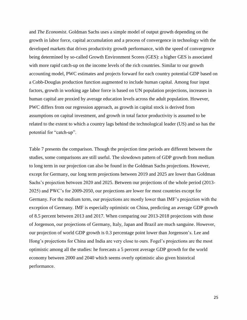
25

and The Economist. Goldman Sachs uses a simple model of output growth depending on the

growth in labor force, capital accumulation and a process of convergence in technology with the

developed markets that drives productivity growth performance, with the speed of convergence

being determined by so-called Growth Environment Scores (GES): a higher GES is associated

with more rapid catch-up on the income levels of the rich countries. Similar to our growth

accounting model, PWC estimates and projects forward for each country potential GDP based on

a Cobb-Douglas production function augmented to include human capital. Among four input

factors, growth in working age labor force is based on UN population projections, increases in

human capital are proxied by average education levels across the adult population. However,

PWC differs from our regression approach, as growth in capital stock is derived from

assumptions on capital investment, and growth in total factor productivity is assumed to be

related to the extent to which a country lags behind the technological leader (US) and so has the

potential for “catch-up”.

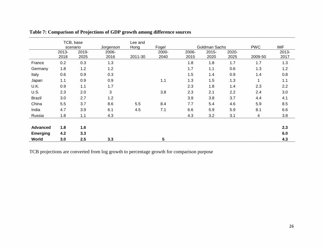
Table 7 presents the comparison. Though the projection time periods are different between the

studies, some comparisons are still useful. The slowdown pattern of GDP growth from medium

to long term in our projection can also be found in the Goldman Sachs projections. However,

except for Germany, our long term projections between 2019 and 2025 are lower than Goldman

Sachs’s projection between 2020 and 2025. Between our projections of the whole period (2013-

2025) and PWC’s for 2009-2050, our projections are lower for most countries except for

Germany. For the medium term, our projections are mostly lower than IMF’s projection with the

exception of Germany. IMF is especially optimistic on China, predicting an average GDP growth

of 8.5 percent between 2013 and 2017. When comparing our 2013-2018 projections with those

of Jorgenson, our projections of Germany, Italy, Japan and Brazil are much sanguine. However,

our projection of world GDP growth is 0.3 percentage point lower than Jorgenson’s. Lee and

Hong’s projections for China and India are very close to ours. Fogel’s projections are the most

optimistic among all the studies: he forecasts a 5 percent average GDP growth for the world

economy between 2000 and 2040 which seems overly optimistic also given historical

performance.

26

Table 7: Comparison of Projections of GDP growth among difference sources

TCB, base scenario Jorgenson

Lee and Hong Fogel Goldman Sachs PWC IMF

2013-2018

2019-2025

2006-2016

2011-30

2000-2040

2006-2015

2015-2020

2020-2025

2009-50

2013-2017

France 0.2 0.3

1.3

1.8 1.8 1.7

1.7

1.3

Germany 1.8 1.2

1.2

1.7 1.1 0.6

1.3

1.2

Italy 0.6 0.9

0.3

1.5 1.4 0.9

1.4

0.8

Japan 1.1 0.9

0.9

1.1

1.3 1.5 1.3

1

1.1

U.K. 0.9 1.1

1.7

2.3 1.8 1.4

2.3

2.2

U.S. 2.3 2.0

3

3.8

2.3 2.1 2.2

2.4

3.0

Brazil 3.0 2.7

1.2

3.9 3.8 3.7

4.4

4.1

China 5.5 3.7

8.6

5.5

8.4

7.7 5.4 4.6

5.9

8.5

India 4.7 3.9

6.1

4.5

7.1

6.6 5.9 5.9

8.1

6.6

Russia 1.8 1.1

4.3

4.3 3.2 3.1

4

3.8

Advanced 1.8 1.6

2.3

Emerging 4.2 3.3

6.0

World 3.0 2.5

3.3

5

4.3

TCB projections are converted from log growth to percentage growth for comparison purpose

27

5. Closing Remarks

The growth accounting framework provides a good starting point for projecting output growth in

the medium and long term. The different methods are strongly dependent on the approach to

estimate capital and TFP growth rates. Does the regression approach provide robust results,

which don’t seem dramatically out of line with other, mostly simpler methods? We believe that

the new methodology combining growth accounting and regression analysis using economic

variables, makes it possible to be more explicit about understanding the sources of growth and

the drivers of change over time.

Our base projections of GDP growth may be seen as relatively low compared with other studies.

However, over a time span as long as the one we have used, there will likely be deviations in

both directions. Despite the transparency and comparability of our approach, the disadvantage is

that there is no simple framework that can take into account all the country specific factors and

potential shocks in the future. That said, our goal is not to provide an explicit forecast in the

sense of the exact growth numbers, but rather to provide a reasonable way of benchmarking

trend growth across a large group of economies. Below are two major directions of the future

work we plan to undertake.

1. The trend growth of labor, capital and productivity are relatively stable factors, although

they require adjustments for cyclical factors for the most recent years and the immediate

future. In the current version of the outlook, we link the short-term growth with medium-

term growth using linear interpolation. Additional research is needed to analyze the path

and timing of the convergence of the short-term growth to trend growth.

2. The growth accounting approach provides projections for the growth of capital services,

TFP and GDP. It is also interesting to examine the level of the potential GDP so that we

can measure the output gap.

28

References

Alcala, Francisco and Antonio Ciccone (2004). “Trade and Productivity,” The Quarterly Journal

of Economics, Vol. 119, No. 2, pp. 613-646.

Bonthuis, Boele (2011). “Constructing a Data Set on Labour Composition Change,” The

Conference Board Economics Program Working Paper Series, December, EPWP#11-04.

Chen, Vivian, Ben Cheng, Gad Levanon and Bart van Ark (2011). “Projecting Economic Growth

with Growth Accounting Techniques: The Conference Board Global Economic Outlook 2012

Sources and Methods,” The Conference Board Economics Program Working Paper Series,

November, EPWP#11-07.

Corrado, Carol, Jonathan Haskel, and Cecilia Jona-Lasinio (2012). "Productivity Growth,

Intangible Capital and ICT: Some International Evidence," forthcoming.

Fogel, Robert W. (2007). “Capitalism and Democracy in 2040: Forecasts and Speculations,”

National Bureau of Economic Research, Working Paper 13184,

http://www.nber.org/papers/w13184.

Gollin, Douglas (2002). “Getting Income Shares Right,” Journal of Political Economy, Vol. 110,

No. 2, pp. 458 – 474.

Hawksworth, John and Anmol Tiwari (2011). “The World in 2050. The Acceleration Shift of

Global Power: Challenges and Opportunities,” PWC.

Heston, Alan, Robert Summers and Bettina Aten, Penn World Table Version 7.0, Center for

International Comparisons of Production, Income and Prices at the University of Pennsylvania,

May 2011.

Horioka, Charles Yuji and Akiko Terada-Hagiwara (2010). “Determinants and Long-term

Projections of Saving Rates in Developing Asia,” ADB Economics Working Paper Series, No.

228.

International Data Base, U.S. Census Bureau,


Jorgenson, Dale W. and Khuong Vu (2008), “Projecting World Economic Growth:

The Contribution of Information Technology”.

Jorgenson, Dale W. and Khuong Vu (2009). “Growth Accounting within the International

Comparison Program,” ICP Bulletin, Vol. 6, No. 1, March, pp. 3-19.

Lee, Jong-Wha and Kiseok Hong (2010). “Economic Growth in Asia: Determinants and

Prospects,” ADB Economics Working Paper Series, No. 220.

http://www.nber.org/papers/w13184


29

Mankiw, Gregory N., David Romer and David N. Weil (1992). “A Contribution to the Empirics

of Economic Growth,” The Quarterly Journal of Economics, Vol. 107, No.2, May, pp.407-437.

Park, Jungsoo (2010). “Projection of Long-Term Total Factor Productivity Growth for 12 Asian

Economies,” ADB Economics Working Paper Series, No. 227.

Shioji, Etsuro and Vu Tuan Khai (2011), “Physical Capital Accumulaiton in Asia-12: Past

Trends and Future Projections,” ADB Economics Working Paper Series, No. 240.

The Conference Board Total Economy Database™, September 2012, http://www.conference-

board.org/data/economydatabase/.

The Conference Board (2012). “Is the Global Economic Speed Limit Slowing Down”

StraightTalk® Series, Vol. 23, No. 3.

Wilson, Dominic and Anna Stupnytska (2007). “The N-11: More Than an Acronym,” Goldman

Sachs Global Economics Paper No: 153.

World Economic Outlook Databases, International Monetary Fund,

http://www.imf.org/external/ns/cs.aspx?id=28

http://www.conference-board.org/data/economydatabase/

http://www.conference-board.org/data/economydatabase/

http://www.imf.org/external/ns/cs.aspx?id=28

30

Appendix

In order to evaluate the accuracy of our projections, we carry out out-of -sample tests on capital

services growth, TFP growth and GDP growth to measure the deviation of the forecast value

from the actual value. Specifically, we use the first four or five periods’ data in simultaneous

equation system to predict capital services and TFP growth in periods 5 or 6. Together with the

labor contribution, we then calculated the projected GDP growth. In the appendix table below,

we list the actual and projected values for capital service growth, TFP growth and GDP growth,

and the corresponding difference between the projected and actual values. Three points worth

noting when reading the numbers in the appendix table:

1. Because we specify lagged variables as explanatory variables in the simultaneous

equation system, the projected capital services growth and TFP growth is affected by the

performance of the previous period. That is why in period 6 (2006 – 2012), which

contains the 2008/09 crisis and on-going European debt crisis, the projected growth is

higher than the actual growth for most advanced economies. This also explains why in

our medium-term projection (2013-2018), the base scenario growth continues the

downward trend. The model specification determines the path dependence nature of the

projection and is not able to forecast any unforeseeable shocks, either negative (such as a

global financial crisis, or the breakup of the euro zone) or positive (such as a strong

acceleration in technological progress and innovation that will lift the world growth out

of the sluggish trajectory). Aware of such limitations, we supplement the projected

growth by optimistic and pessimistic scenarios, in which capital services growth and TFP

growth deviate from the model projections to reflect the possible upside and downside

risks (see section 3).

2. The deviation between the projected GDP growth and actual GDP growth for period 5 &

6 comes not only from the differences in the projected and actual capital services growth

and TFP growth. It is also partially due to the fact that in our projected GDP growth, we

approximate the actual employment growth by the growth in working age population.

The discrepancy will be especially evident in countries with volatile labor participation

rate and employment rate.

31

3. Our medium and long-term projections for China and India may seem low compared with

the actual GDP growth in the past decades in these two countries. However, when

comparing with the projections in period 5 and 6, these projections indicate a gradual

slowdown in China and India instead of a sudden drop from 2013 and onwards. Take

China for example, the projected GDP growth for periods 5 to 8 is 7.5 percent, 6.8

percent, 4.9 percent and 3.6 percent, respectively. It is a result of combined slowdown in

all of the input factors. Specifically, China will run out of the demographic dividend

during 2013-2018 as its working age population growth will decline; capital services

growth gradually slow down as the return to capital declines after many years of intensive

investment and the economy is shifting towards a more consumption driven growth

model; last but not the least, productivity growth weakens as the country matures and the

easy productivity gains from learning the leaders exhaust and future productivity growth

has to originate from technological progress and innovation.

32

Appendix Table: Actual and projected growth of capital services, TFP and GDP, and the

differences

Period 5 (1999-2005)

Capital services growth (%) TFP growth (%) GDP growth (%)

country Actual Projected

Difference (Projected - Actual)

Actual Projected

Difference (Projected -

Actual)

Actual Projected


Actual)

Advanced Economies


0.9 0.5 -0.3

2.9 3.0 0.1

Austria 2.7 3.5 0.8

0.7 1.0 0.3

2.2 2.6 0.4

Belgium 3.7 3.8 0.2

0.1 1.3 1.2

2.1 3.0 0.8

Cyprus 1.1 1.6 0.5

1.5 1.4 0.0

3.6 4.0 0.4

Czech Republic 5.3 4.8 -0.5

1.5 1.8 0.3

3.7 4.3 0.6

Denmark 3.6 3.3 -0.3

0.1 1.0 0.8

1.7 2.3 0.6

Finland 3.2 4.2 1.0

1.2 0.9 -0.3

3.1 2.7 -0.4

France 3.7 1.0 -2.7

0.2 0.8 0.6

2.1 1.8 -0.4

Germany 1.8 3.9 2.1

0.8 1.0 0.2

1.1 2.1 0.9

Greece 5.6 2.1 -3.5

0.1 1.0 0.9

3.9 2.7 -1.2

Hungary 6.8 3.9 -2.9

0.5 1.5 1.0

4.0 3.7 -0.3

Ireland 7.7 7.3 -0.4

0.4 1.6 1.1

6.1 6.5 0.4

Italy 2.8 3.7 0.9

-0.4 0.7 1.1

1.4 2.4 0.9

Luxembourg 5.1 2.7 -2.5

0.8 1.8 1.0

4.8 3.9 -0.9

Malta 1.0 3.2 2.1

0.2 1.8 1.6

1.0 3.8 2.7


0.5 1.3 0.9

2.1 3.0 0.9

Norway 3.8 1.8 -2.0

0.3 0.9 0.6

2.3 2.3 0.0

Poland 4.1 3.2 -0.9

1.3 1.4 0.0

3.4 3.4 0.0

Portugal 5.4 3.7 -1.7

-2.1 1.0 3.2

1.7 3.3 1.6

Spain 4.9 3.8 -1.2

-0.7 0.9 1.6

3.7 3.6 -0.1

Sweden 3.3 4.6 1.3

1.5 1.4 -0.1

3.2 3.6 0.4


0.2 1.2 1.0

1.6 2.8 1.2

United Kingdom 4.6 4.1 -0.5

0.8 0.8 0.0

3.1 3.1 0.0

Japan 1.5 3.2 1.7

0.6 1.1 0.5

1.1 2.7 1.6

Australia 5.1 3.2 -1.9

0.1 1.0 0.9

3.4 3.4 0.0

Canada 4.3 3.7 -0.6

0.3 1.2 0.9

3.3 3.6 0.3

Hong Kong 3.6 1.6 -1.9

2.1 2.9 0.8

4.4 4.3 0.0

Iceland 4.1 2.3 -1.8

2.0 1.2 -0.8

4.2 3.2 -0.9

Israel 4.4 5.4 0.9

0.3 1.4 1.0

3.2 5.1 1.9


0.2 1.4 1.1

3.7 4.3 0.5


3.2 3.0 -0.2

5.4 7.6 2.2

South Korea 5.9 5.3 -0.6

2.9 1.4 -1.4

5.8 3.8 -2.0

Taiwan 5.8 4.7 -1.1

1.5 1.3 -0.2

4.2 4.0 -0.1

33

Period 5 (1999-2005)




Actual Projected


Actual)

Actual Projected


Actual)


China 10.6 7.8 -2.8

4.1 2.6 -1.5

10.1 7.5 -2.6

India 6.6 5.2 -1.4

1.9 0.9 -0.9

6.3 4.6 -1.7

Indonesia 4.3 7.1 2.8

1.3 1.3 0.0

4.1 5.9 1.8


2.2 2.1 -0.1

5.4 7.4 2.1

Pakistan 4.0 5.2 1.2

1.6 0.6 -0.9

4.8 4.9 0.1


2.5 2.1 -0.5

5.1 6.2 1.1

Argentina 1.2 3.6 2.4

-0.8 1.0 1.8

0.4 3.5 3.1

Brazil 2.9 3.9 0.9

-0.5 0.8 1.3

2.6 3.8 1.2

Chile 6.0 3.7 -2.3

-1.6 1.7 3.3

3.7 4.7 1.0

Colombia 2.8 3.4 0.6

-0.8 1.0 1.8

2.3 3.8 1.5

Mexico 4.0 3.7 -0.3

-0.5 1.1 1.6

2.8 4.2 1.5

Venezuela 0.9 3.6 2.7

0.2 0.8 0.6

1.4 3.8 2.3

Iran 2.7 2.3 -0.3

0.9 0.4 -0.6

5.2 3.3 -1.9

Saudi Arabia 3.2 3.4 0.2

-1.1 0.0 1.1

3.2 3.5 0.3

United Arab Emirates 3.7 4.5 0.8

1.6 0.4 -1.2

7.1 5.5 -1.6

Algeria 1.3 2.2 0.9

2.0 1.0 -1.1

4.2 3.7 -0.5

Egypt 3.0 6.3 3.3

0.6 1.2 0.6

4.2 6.1 1.9

Morocco 4.4 5.4 1.0

0.6 1.6 0.9

3.8 5.5 1.7

Nigeria 3.2 3.5 0.4

5.5 -0.6 -6.1

8.3 2.5 -5.8

South Africa 4.4 4.7 0.2

-0.4 -1.4 -1.0

3.6 2.1 -1.5

Russian Federation -1.6 1.1 2.8

6.7 0.7 -6.0

6.5 1.4 -5.1

Turkey 5.8 3.9 -1.9

0.7 0.5 -0.1

3.6 3.9 0.2

34

Period 6 (2006-2012)



Difference (Projected - Actual) Actual Projected



Advanced Economies


0.1 0.7 0.6

1.0 2.9 1.8

Austria 1.8 3.5 1.7

0.6 0.7 0.1

1.5 2.0 0.6

Belgium 2.8 4.2 1.3

-0.5 1.3 1.8

1.2 2.9 1.8

Cyprus 2.4 1.9 -0.5

-0.1 0.9 1.0

1.4 3.3 1.8

Czech Republic 4.1 4.8 0.7

0.3 2.4 2.1

2.1 4.1 2.1

Denmark 2.8 4.3 1.5

-0.7 0.9 1.6

0.1 2.3 2.1

Finland 3.5 3.9 0.5

-0.7 0.8 1.5

1.1 2.2 1.1

France 3.1 0.9 -2.2

-0.7 0.4 1.2

0.7 1.1 0.4

Germany 1.7 4.4 2.8

0.4 1.2 0.8

1.5 2.7 1.2

Greece 3.3 3.6 0.3

-2.0 0.7 2.7

-1.6 2.6 4.2

Hungary 4.2 5.0 0.8

-1.7 2.2 3.9

-0.1 4.3 4.5

Ireland 4.8 5.8 1.0

-0.9 1.5 2.4

0.1 4.8 4.7

Italy 1.4 3.8 2.4

-0.8 0.3 1.1

-0.4 1.9 2.3

Luxembourg 4.4 2.1 -2.3

-1.8 2.1 3.9

1.6 3.9 2.3

Malta 0.4 3.1 2.7

1.0 1.6 0.6

2.1 3.3 1.2


-0.1 1.3 1.4

1.0 2.6 1.6

Norway 4.4 1.8 -2.6

-2.2 0.9 3.1

1.1 2.2 1.1

Poland 4.9 3.7 -1.2

0.9 1.3 0.4

4.3 3.4 -0.9

Portugal 2.9 3.5 0.6

-1.2 0.6 1.7

-0.4 2.4 2.8

Spain 3.7 3.4 -0.2

-0.8 0.6 1.4

0.4 2.7 2.3

Sweden 3.5 4.7 1.2

-0.3 1.2 1.5

1.7 2.9 1.2


0.2 0.9 0.8

1.9 3.0 1.0

United Kingdom 2.7 4.0 1.3

-0.4 0.3 0.7

0.4 2.0 1.5

Japan 0.7 3.0 2.3

0.4 0.7 0.4

0.4 1.7 1.4

Australia 6.2 4.1 -2.1

-1.4 0.7 2.1

2.7 3.3 0.5

Canada 3.8 3.7 -0.1

-0.8 1.1 1.8

1.5 3.2 1.7

Hong Kong 3.0 1.5 -1.6

2.2 3.4 1.2

3.7 4.5 0.8

Iceland -2.7 1.3 4.0

1.4 0.8 -0.6

0.9 2.2 1.2

Israel 4.2 5.6 1.5

0.1 1.3 1.3

4.0 4.9 0.9


-1.3 1.3 2.7

1.2 4.1 2.9


0.1 3.1 3.0

5.5 6.9 1.4

South Korea 5.2 4.9 -0.3

1.8 1.5 -0.3

3.6 3.6 0.0

Taiwan 2.9 4.5 1.6 1.8 1.5 -0.3 3.6 4.1 0.5

35

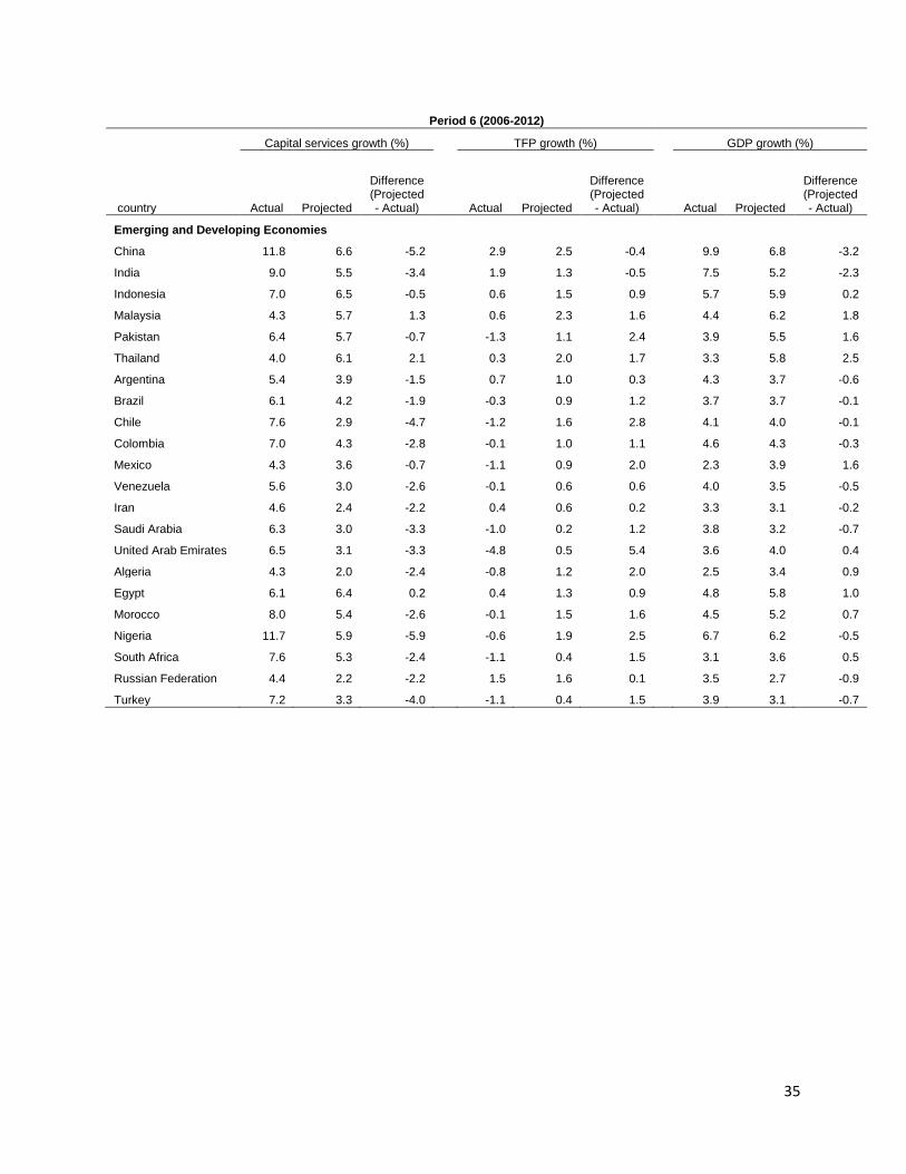
Period 6 (2006-2012)







China 11.8 6.6 -5.2

2.9 2.5 -0.4

9.9 6.8 -3.2

India 9.0 5.5 -3.4

1.9 1.3 -0.5

7.5 5.2 -2.3

Indonesia 7.0 6.5 -0.5

0.6 1.5 0.9

5.7 5.9 0.2


0.6 2.3 1.6

4.4 6.2 1.8

Pakistan 6.4 5.7 -0.7

-1.3 1.1 2.4

3.9 5.5 1.6


0.3 2.0 1.7

3.3 5.8 2.5

Argentina 5.4 3.9 -1.5

0.7 1.0 0.3

4.3 3.7 -0.6

Brazil 6.1 4.2 -1.9

-0.3 0.9 1.2

3.7 3.7 -0.1

Chile 7.6 2.9 -4.7

-1.2 1.6 2.8

4.1 4.0 -0.1

Colombia 7.0 4.3 -2.8

-0.1 1.0 1.1

4.6 4.3 -0.3

Mexico 4.3 3.6 -0.7

-1.1 0.9 2.0

2.3 3.9 1.6

Venezuela 5.6 3.0 -2.6

-0.1 0.6 0.6

4.0 3.5 -0.5

Iran 4.6 2.4 -2.2

0.4 0.6 0.2

3.3 3.1 -0.2

Saudi Arabia 6.3 3.0 -3.3

-1.0 0.2 1.2

3.8 3.2 -0.7

United Arab Emirates 6.5 3.1 -3.3

-4.8 0.5 5.4

3.6 4.0 0.4

Algeria 4.3 2.0 -2.4

-0.8 1.2 2.0

2.5 3.4 0.9

Egypt 6.1 6.4 0.2

0.4 1.3 0.9

4.8 5.8 1.0

Morocco 8.0 5.4 -2.6

-0.1 1.5 1.6

4.5 5.2 0.7

Nigeria 11.7 5.9 -5.9

-0.6 1.9 2.5

6.7 6.2 -0.5

South Africa 7.6 5.3 -2.4

-1.1 0.4 1.5

3.1 3.6 0.5

Russian Federation 4.4 2.2 -2.2

1.5 1.6 0.1

3.5 2.7 -0.9

Turkey 7.2 3.3 -4.0 -1.1 0.4 1.5 3.9 3.1 -0.7

Documents

Projecting Global Growth - Trusted Insights for Business ... · PDF fileProjecting Global Growth by Vivian Chen, ... mature and 22 emerging market economies for 2013, ... The trend