Embed Size (px)
Citation preview
HAL Id: tel-00332787https://pastel.archives-ouvertes.fr/tel-00332787
Submitted on 21 Oct 2008
HAL is a multi-disciplinary open accessarchive for the deposit and dissemination of sci-entific research documents, whether they are pub-lished or not. The documents may come fromteaching and research institutions in France orabroad, or from public or private research centers.
L’archive ouverte pluridisciplinaire HAL, estdestinée au dépôt et à la diffusion de documentsscientifiques de niveau recherche, publiés ou non,émanant des établissements d’enseignement et derecherche français ou étrangers, des laboratoirespublics ou privés.
Projections in several complex variablesChin-Yu Hsiao
To cite this version:Chin-Yu Hsiao. Projections in several complex variables. Mathematics [math]. Ecole PolytechniqueX, 2008. English. tel-00332787
These de Doctorat de Chin-Yu Hsiao sous
la direction du Prof. J. Sjostrand
PROJECTEURS ENPLUSIEURSVARIABLES COMPLEXES

Chin-Yu Hsiao
CMLS, Ecole Polytechnique, 91128 Palaiseau Cedex, France UMR 7640.
E-mail : [email protected]
These presentee pour obtenir le titre de
DOCTEUR DE L’ECOLE POLYTECHNIQUE
specialite: Mathematiques
par
Chin-Yu HSIAO
Projecteurs en Plusieurs
Variables Complexes
Projections in Several Complex Variables
Directeur de these: Johannes SJOSTRAND
Soutenue le 2 juillet 2008 devant le jury compose de
MM. Robert Berman
Bo Berndtsson
Louis Boutet de Monvel
Bernard Helffer
Xiaonan Ma
Johannes Sjostrand
Claude Viterbo
Examinateur
Rapporteur(absent)
Rapporteur
President du jury
Rapporteur
Directeur de these
Examinateur

Remerciements
Je voudrais, en tout premier lieu, exprimer toute ma gratitude à Johannes
Sjöstrand, mon directeur de thèse, non seulement pour sa génerosité et son sou-
tien au cours de ces trois années, mais aussi pour son excellente direction à la
fois avisée et exigeante à laquelle cette thèse doit beaucoup. C’est grâce à lui que
j’ai pu découvrir le domaine de l’analyse microlocale appliquée à l’analyse com-
plexe et le monde de la recherche. J’ai eu beaucoup de plaisir à être son étudiant.
J’aimerais aussi remercier Louis Boutet de Monvel pour sa lecture et les ex-
plications, suggestions et discussions qu’il m’a apportées, Bo Berndtsson pour sa
lecture et remarques et Xiaonan Ma pour sa lecture détaillée et ses corrections.
Je remercie Claude Viterbo, Bernard Helffer et Robert Berman de m’avoir fait
un grand honneur d’être membres de mon jury.
Je tiens à exprimer ma reconnaissance à Bo Berndtsson et Robert Berman
pour avoir fait de ma visit à l’Université de Göteborg en novembre-decembre
2006 un moment inoubliable et pour les discussions qu’on a eu pendant mon
séjour en Suède, qui ont été toutes très utiles.
Cette thèse a été effectuée au Centre de Mathématiques Laurent Schwartz
(CMLS) de l’Ecole Polytechnique, un laboratoire extrêmement accueillant et cha-
leureux dont je voudrais remercier tous les membres.


This Thesis consists of an introduction and the following papers:
Paper I: On the singularities of the Szegö projection for (0,q ) forms
Paper II: On the singularities of the Bergman projection for (0,q ) forms

Introduction
The Bergman and Szegö projections are classical subjects in several com-plex variables and complex geometry. By Kohn’s regularity theorem for the ∂ -Neumann problem (1963, [11]), the boundary behavior of the Bergman kernel ishighly dependent on the Levi curvature of the boundary. The study of the bound-ary behavior of the Bergman kernel on domains with positive Levi curvature(strictly pseudoconvex domains) became an important topic in the field then. In1965, L. Hörmander ([9]) determined the boundary behavior of the Bergman ker-nel. C. Fefferman (1974, [7]) established an asymptotic expansion at the diagonalof the Bergman kernel. More complete asymptotics of the Bergman kernel wasobtained by Boutet de Monvel and Sjöstrand (1976, [6]). They also established anasymptotic expansion of the Szegö kernel on strongly pseudoconvex boundaries.All these developments concerned pseudoconvex domains. For the nonpseudo-convex domain, there are few results. R. Beals and P. Greiner (1988, [1]) provedthat the Szegö projection is a Heisenberg pseudodifferential operator, under cer-tain Levi curvature assumptions. Hörmander (2004, [10]) determined the bound-ary behavior of the Bergman kernel when the Levi form is negative definite bycomputing the leading term of the Bergman kernel on a spherical shell in Cn .
Other developments recently concerned the Bergman kernel for a high powerof a holomorphic line bundle. D. Catlin (1997, [4]) and S. Zelditch (1998, [16])adapted a result of Boutet de Monvel-Sjöstrand for the asymptotics of the Szegökernel on a strictly pseudoconvex boundary to establish the complete asymp-totic expansion of the Bergman kernel for a high power of a holomorphic linebundle with positive curvature. Recently, a new proof of the existence of thecomplete asymptotic expansion was obtained by B. Berndtsson, R. Berman andJ. Sjöstrand (2004, [3]). Without the positive curvature assumption, R. Bermanand J. Sjöstrand (2005, [2]) obtained a full asymptotic expansion of the Bergmankernel for a high power of a line bundle when the curvature is non-degenerate.The approach of Berman and Sjöstrand builds on the heat equation method ofMenikoff-Sjöstrand (1978, [15]). The expansion was obtained independently byX. Ma and G. Marinescu (2006, [14]) (without a phase function) by using a spec-tral gap estimate for the Hodge Laplacian.
Recently, Hörmander (2004, [10]) studied the Bergman projection for (0,q )forms. In that paper (page 1306), Hörmander suggested: "A carefull microlocalanalysis along the lines of Boutet de Monvel-Sjöstrand should give the asymp-
1
totic expansion of the Bergman projection for (0,q ) forms when the Levi form isnon-degenerate."
The main goal for this thesis is to achieve Hörmander’s wish-more precisely,to obtain an asymptotic expansion of the Bergman projection for (0,q ) forms.The first step of my research is to establish an asymptotic expansion of the Szegöprojection for (0,q ) forms. Then, find a suitable operator defined on the bound-ary of domain which plays the same role as the Kohn Laplacian in the approachof Boutet de Monvel-Sjöstrand.
This thesis consists two parts. In the first paper, we completely study theheat equation method of Menikoff-Sjöstrand and apply it to the Kohn Laplaciandefined on a compact orientable connected CR manifold. We then get the fullasymptotic expansion of the Szegö projection for (0,q ) forms when the Levi formis non-degenerate. We also compute the leading term of the Szegö projection.
In the second paper, we introduce a new operator analogous to the KohnLaplacian defined on the boundary of a domain and we apply the method ofMenikoff-Sjöstrand to this operator. We obtain a description of a new Szegö pro-jection up to smoothing operators. Finally, by using the Poisson operator, we getthe full asymptotic expansion of the Bergman projection for (0,q ) forms whenthe Levi form is non-degenerate.
In order to describe the results more precisely, we introduce some notations.Let Ω be a C∞ paracompact manifold equipped with a smooth density of inte-gration. We let T (Ω) and T ∗(Ω) denote the tangent bundle ofΩ and the cotangentbundle ofΩ respectively. The complexified tangent bundle ofΩ and the complex-ified cotangent bundle of Ω will be denoted by CT (Ω) and CT ∗(Ω) respectively.We write ⟨ , ⟩ to denote the pointwise duality between T (Ω) and T ∗(Ω). We extend⟨ , ⟩ bilinearly to CT (Ω)×CT ∗(Ω).
Let E be a C∞ vector bundle over Ω. The spaces of smooth sections of E overΩ and distribution sections of E over Ωwill be denoted by C∞(Ω; E ) andD ′(Ω; E )respectively. Let E ′(Ω; E ) be the subspace of D ′(Ω; E ) of sections with compactsupport in Ω and let C∞0 (Ω; E ) =C∞(Ω; E )
⋂
E ′(Ω; E ).Let C , D be C∞ vector bundles over Ω. Let
A : C∞0 (Ω; C )→D ′(Ω; D).
From now on, we write KA(x , y ) or A(x , y ) to denote the distribution kernel of A.Let
B : C∞0 (Ω; C )→D ′(Ω; D).
We writeA ≡ B
ifKA(x , y ) = K B (x , y )+ F (x , y ),
where F (x , y )∈C∞(Ω×Ω;L (Cy , Dx )).
2
0.1 The Szegö projection
For the precise definitions of some standard notations in CR geometry, see sec-tion 2 of paper I . Let (X ,Λ1,0T (X )) be a compact orientable connected CR mani-fold of dimension 2n−1, n ≥ 2. We take a smooth Hermitian metric ( | ) onCT (X )so that Λ1,0T (X ) is orthogonal to Λ0,1T (X ) and (u | v ) is real if u , v are real tangentvectors, where Λ0,1T (X ) = Λ1,0T (X ). The Hermitian metric ( | ) on CT (X ) induces,by duality, a Hermitian metric on CT ∗(X ) that we shall also denote by ( | ). Forq ∈ N, let Λ0,q T ∗(X ) be the bundle of (0,q ) forms of X . The Hermitian metric ( | )on CT ∗(X ) induces a Hermitian metric on Λ0,q T ∗(X ) also denoted by ( | ).
We take (d m ) as the induced volume form on X and let ( | ) be the inner prod-uct on C∞(X ; Λ0,q T ∗(X )) defined by
( f | g ) =∫
X
( f (z ) | g (z ))(d m ), f , g ∈C∞(X ; Λ0,q T ∗(X )).
Since X is orientable, there is a globally defined real 1 form ω0(z ) of lengthone which is pointwise orthogonal to Λ1,0T ∗(X )⊕Λ0,1T ∗(X ), where
Λ1,0T ∗(X ) = Λ0,1T ∗(X ).
There is a real non-vanishing vector field Y which is pointwise orthogonal toΛ1,0T (X )⊕Λ0,1T (X ). We take Y so that
⟨Y ,ω0⟩=−1, ‖Y ‖= 1.
The Levi form L p (Z , W ), p ∈ X , Z , W ∈ Λ1,0Tp (X ), is the Hermitian quadraticform on Λ1,0Tp (X ) defined as follows:
For any Z , W ∈Λ1,0Tp (X ), pick eZ , fW ∈C∞(X ; Λ1,0T (X )) that satisfy
eZ (p ) =Z , fW (p ) =W . Then L p (Z , W ) =1
2i
D
[eZ ,fW ](p ) ,ω0(p )E
.(0.1)
The eigenvalues of the Levi form at p ∈ X are the eigenvalues of the Hermitianform L p with respect to the inner product ( | ) on Λ1,0Tp (X ).
Let b be the Kohn Laplacian on X and let (q )b denote the restriction to (0,q )forms. Let
π(q ) : L2(X ; Λ0,q T ∗(X ))→Ker(q )b
be the Szegö projection, i.e. the orthogonal projection onto the kernel of(q )b . Let
Kπ(q )(x , y )∈D ′(X ×X ;L (Λ0,q T ∗y (X ),Λ0,q T ∗x (X )))
be the distribution kernel of π(q ) with respect to (d m ). Formally,
(π(q )u )(x ) =
∫
Kπ(q )(x , y )u (y )d m (y ), u (y )∈C∞(X ; Λ0,q T ∗(X )).
We recall
3
Definition 0.1. Given q , 0 ≤ q ≤ n − 1, the Levi form is said to satisfy conditionY (q ) at p ∈ X if for any |J |= q , J = (j1, j2, . . . , jq ), 1≤ j1 < j2 < · · ·< jq ≤ n − 1, wehave
∑
j /∈J
λj −∑
j∈J
λj
<n−1∑
j=1
λj
,
where λj , j = 1, . . . , (n − 1), are the eigenvalues of L p . If the Levi form is non-degenerate at p , then the condition is equivalent to q 6= n+, n−, where (n−, n+),n−+n+ = n −1, is the signature of L p .
When Y (q ) holds at each point of X , Kohn (1972, [8]) proved that
Kπ(q )(x , y )∈C∞(X ×X ;L (Λ0,q T ∗(X ),Λ0,q T ∗(X ))).
When condition Y (q ) fails, one is interested in the Szegö projection on the level of(0,q ) forms. If the Levi form is positive definite at each point of X , Boutet de Mon-vel and Sjöstrand (1976, [6]) obtained the full asymptotic expansion for Kπ(0)(x , y ).If Y (q ) fails, Y (q−1), Y (q+1) hold and the Levi form is non-degenerate, Beals andGreiner (1988, [1]) proved that π(q ) is a Heisenberg pseudodifferential operator.In particular, π(q ) is a pseudodifferential operator of order 0 type ( 1
2, 1
2).
The statement of the main results of paper I
Let Σ be the characteristic manifold of (q )b . We have
Σ=
(x ,ξ)∈ T ∗(X ) \0; ξ=λω0(x ),λ 6= 0
.
Put
Σ+ =
(x ,ξ)∈ T ∗(X ) \0; ξ=λω0(x ),λ> 0
,
Σ− =
(x ,ξ)∈ T ∗(X ) \0; ξ=λω0(x ),λ< 0
.
We assume that the Levi form is non-degenerate at each point of X . Then theLevi form has constant signature (n−, n+), n−+n+ = n −1. We define
Σ = Σ+ if n+ =q 6= n−,
Σ = Σ− if n− =q 6= n+,
Σ = Σ+⋃
Σ− if n+ =q = n−.
The main result of the first paper is the following
Theorem 0.2. Let (X ,Λ1,0T (X )) be a compact orientable connected CR manifold ofdimension 2n − 1, n ≥ 2, with a Hermitian metric ( | ). We assume that the Leviform L is non-degenerate at each point of X . Then, the Levi form has constant
4
signature (n−, n+), n− + n+ = n − 1. Let q = n− or n+. Suppose (q )b has closedrange. Then π(q ) is a well defined continuous operator
π(q ) : H s (X ; Λ0,q T ∗(X ))→H s (X ; Λ0,q T ∗(X )),
for all s ∈R, andWF ′(Kπ(q )) = diag (Σ× Σ),
where H s , s ∈R, is the standard Sobolev space of order s and
WF ′(Kπ(q )) =
(x ,ξ, y ,η)∈ T ∗(X )×T ∗(X ); (x ,ξ, y ,−η)∈WF (Kπ(q ))
.
Here WF (Kπ(q )) is the wave front set of Kπ(q ) in the sense of Hörmander (see Ap-pendix A of the second paper for a review). Moreover, we have
Kπ(q ) = Kπ+ if n+ =q 6= n−,
Kπ(q ) = Kπ− if n− =q 6= n+,
Kπ(q ) = Kπ+ +Kπ− if n+ =q = n−,
where Kπ+(x , y ) satisfies
Kπ+(x , y )≡∫ ∞
0
e iφ+(x ,y )t s+(x , y , t )d t
withs+(x , y , t )∈Sn−1
1,0 (X ×X×]0,∞[;L (Λ0,q T ∗y (X ),Λ0,q T ∗x (X ))),
s+(x , y , t )∼∞∑
j=0
s j+(x , y )t n−1−j
in the symbol space Sn−11,0 (X ×X×]0,∞[;L (Λ0,q T ∗y (X ),Λ
0,q T ∗x (X ))),
where Sm1,0, m ∈ R, is the Hörmander symbol space (see Appendix A of the first
paper for a review and references),
s j+(x , y )∈C∞(X ×X ;L (Λ0,q T ∗y (X ),Λ
0,q T ∗x (X ))), j = 0, 1, . . . ,
and
φ+(x , y )∈C∞(X ×X ), (0.2)
φ+(x ,x ) = 0, (0.3)
φ+(x , y ) 6= 0 if x 6= y , (0.4)
Imφ+(x , y )≥ 0, (0.5)
d xφ+ 6= 0, d yφ+ 6= 0 where Imφ+ = 0, (0.6)
d xφ+(x , y )|x=y =ω0(x ), (0.7)
d yφ+(x , y )|x=y =−ω0(x ), (0.8)
φ+(x , y ) =−φ+(y ,x ). (0.9)
5
Similarly,
Kπ−(x , y )≡∫ ∞
0
e iφ−(x ,y )t s−(x , y , t )d t
with
s−(x , y , t )∈Sn−11,0 (X ×X×]0,∞[;L (Λ0,q T ∗y (X ),Λ
0,q T ∗x (X ))),
s−(x , y , t )∼∞∑
j=0
s j−(x , y )t n−1−j
in the symbol space Sn−11,0 (X ×X×]0,∞[;L (Λ0,q T ∗y (X ),Λ
0,q T ∗x (X ))),
wheres j−(x , y )∈C∞(X ×X ;L (Λ0,q T ∗y (X ),Λ
0,q T ∗x (X ))), j = 0, 1, . . . ,
and −φ−(x , y ) satisfies (0.2)-(0.9).More properties of the phase φ+(x , y ) will be given in Theorem 0.4 and Re-
mark 0.5 below.
Remark 0.3. We notice that if Y (q − 1) and Y (q + 1) hold then (q )b has closedrange.
The tangential Hessian ofφ+(x , y )
Until further notice, we assume that the Levi form is non-degenerate at eachpoint of X . The phaseφ+(x , y ) is not unique. we can replaceφ+(x , y ) by
eφ(x , y ) = f (x , y )φ+(x , y ), (0.10)
where f (x , y )∈C∞(X×X ) is real and f (x ,x ) = 1, f (x , y ) = f (y ,x ). Then eφ satisfies(0.2)-(0.9). We work with local coordinates x = (x1, . . . ,x2n−1) defined on an openset Ω⊂X . We want to know the Hessian
(φ+)′′ =
(φ+)′′x x (φ+)′′x y
(φ+)′′y x (φ+)′′y y
of φ+ at (p , p ) ∈ X ×X . Let U , V ∈ CTp (X )×CTp (X ). From (0.10), we can checkthat¬
eφ′′(p , p )U , V¶
=
(φ+)′′(p , p )U , V
+
d f (p , p ),U
dφ+(p , p ), V
+
d f (p , p ), V
dφ+(p , p ),U
.
Thus, the Hessian (φ+)′′ ofφ+ at (p , p ) is only well-defined on the space
T(p ,p )H+ =¦
W ∈CTp (X )×CTp (X );
dφ+(p , p ), W
= 0©
.
6
In view of (0.7) and (0.8), we see that T(p ,p )H+ is spanned by
(u , v ), (Y (p ), Y (p )), u , v ∈Λ1,0Tp (X )⊕Λ0,1Tp (X ).
We define the tangential Hessian ofφ+(x , y ) at (p , p ) as the bilinear map:
T(p ,p )H+×T(p ,p )H+→C,
(U , V )→¬
(φ′′+)(p , p )U , V¶
, U , V ∈ T(p ,p )H+.
In the section 9 of the first paper, we completely determined the tangential Hes-sian of φ+(x , y ) at (p , p ). For the better understanding, we describe it in somespecial local coordinates. For a given point p ∈X , let
U1(x ), . . . ,Un−1(x )
be an orthonormal frame ofΛ1,0Tx (X ) varying smoothly with x in a neighborhoodof p , for which the Levi form is diagonalized at p . We take local coordinates
x = (x1, . . . ,x2n−1), z j = x2j−1+ i x2j , j = 1, . . . , n −1,
defined on some neighborhood of p such that
ω0(p ) =p
2d x2n−1, x (p ) = 0,
(∂
∂ x j(p ) |
∂
∂ xk(p )) = 2δj ,k , j , k = 1, . . . , 2n −1
and
Uj =∂
∂ z j−
1p
2a j (x )
∂
∂ x2n−1+
2n−2∑
s=1
c j ,s (x )∂
∂ xs, j = 1, . . . , n −1,
where∂
∂ z j=
1
2(∂
∂ x2j−1− i
∂
∂ x2j), j = 1, . . . , n −1,
a j ∈C∞, a j (0) = 0, j = 1, . . . , n −1 and
c j ,s (x )∈C∞, c j ,s (0) = 0, j = 1, . . . , n −1, s = 1, . . . , 2n −2.
The integrability of Λ1,0T (X ), i.e. [Uj ,Uk ]∈Λ1,0T (X ) implies that
∂ a j
∂ z k(0) =
∂ a k
∂ z j(0), j , k = 1, . . . , n −1. (0.11)
Since the Levi form is diagonalized at p with respect to Uj (p ), j = 1, . . . , n −1, wecan check that (see (0.1))
∂ a j
∂ z k(0)−
∂ a k
∂ z j(0) = 2iλjδj ,k , j , k = 1, . . . , n −1, (0.12)
7
where λj , j = 1, . . . , n −1, are the eigenvalues of L p .If φ ∈ C∞(X ×X ), φ(p , p ) = 0, d x ,y φ(p , p ) = d x ,yφ+(p , p ) and the tangential
Hessian of φ(x , y ) at (p , p ) is the same as the tangential Hessian of φ+(x , y ) at(p , p ), then
φ(x , y ′,x2n−1)−φ+(x , y ′,x2n−1) =O(
(x , y ′)
3)
in some neighborhood of (p , p ), where y ′ = (y1, . . . , y2n−2). Moreover, we have thefollowing
Theorem 0.4. With the notations used before, in some neighborhood of (p , p ) ∈X ×X , we have
φ+(x , y ) =p
2(x2n−1− y2n−1)+ in−1∑
j=1
λj
z j −w j
2+
1
2
n−1∑
j ,k=1
∂ a j
∂ z k(0)(z j z k −w j wk )
+∂ a j
∂ z k(0)(z j z k −w j w k )+
∂ a j
∂ z k(0)(z j z k −w j w k )+
∂ a j
∂ z k(0)(z j z k −w j wk )
+n−1∑
j=1
iλj (z j w j − z j w j )+∂ a j
∂ x2n−1(0)(z j x2n−1−w j y2n−1)
+∂ a j
∂ x2n−1(0)(z j x2n−1−w j y2n−1)
+p
2(x2n−1− y2n−1) f (x , y )+O(
(x , y )
3),
f ∈C∞, f (0, 0) = 0, f (x , y ) = f (y ,x ),
y = (y1, . . . , y2n−1), w j = y2j−1+ i y2j , j = 1, . . . , n −1, (0.13)
where λj , j = 1, . . . , n −1, are the eigenvalues of L p andφ+ is as in Theorem 0.2.
Remark 0.5. We use the same notations as in Theorem 0.4. Since
∂ φ+
∂ x2n−1(0, 0) 6= 0,
from the Malgrange preparation theorem (see Theorem B.6 of the first paper),we have
φ+(x , y ) = g (x , y )(p
2x2n−1+h(x ′, y ))
in some neighborhood of (0, 0), where g , h ∈ C∞, g (0, 0) = 1, h(0, 0) = 0 andx ′ = (x1, . . . ,x2n−2). Put
φ(x , y ) =p
2x2n−1+h(x ′, y ).
From the global theory of Fourier integral operators (see Proposition B.21 of thefirst paper), we see that φ+(x , y ) and φ(x , y ) are equivalent at (p ,ω0(p )) in thesense of Melin-Sjöstrand (see Definition B.20 of the first paper). Sinceφ+(x , y ) =−φ+(y ,x ), we can replaceφ+(x , y ) by
φ(x , y )− φ(y ,x )2
.
8
Thenφ+(x , y ) satisfies (0.2)-(0.9). Moreover, we can check that
φ+(x , y ) =p
2(x2n−1− y2n−1)+ in−1∑
j=1
λj
z j −w j
2+
1
2
n−1∑
j ,k=1
∂ a j
∂ z k(0)(z j z k −w j wk )
+∂ a j
∂ z k(0)(z j z k −w j w k )+
∂ a j
∂ z k(0)(z j z k −w j w k )+
∂ a j
∂ z k(0)(z j z k −w j wk )
+n−1∑
j=1
iλj (z j w j − z j w j )+∂ a j
∂ x2n−1(0)(z j x2n−1−w j y2n−1)
+∂ a j
∂ x2n−1(0)(z j x2n−1−w j y2n−1)
+O(
(x , y )
3), (0.14)
where λj , j = 1, . . . , n−1, are the eigenvalues of L p . (Compare (0.14) with (0.13).)
The leading term of the Szegö projection
We have the following corollary of Theorem 0.2.
Corollary 0.6. There exist smooth functions
F+,G+, F−,G− ∈C∞(X ×X ; L (Λ0,q T ∗y (X ),Λ0,q T ∗x (X )))
such that
Kπ+ = F+(−i (φ+(x , y )+ i 0))−n +G+ log(−i (φ+(x , y )+ i 0)),
Kπ− = F−(−i (φ−(x , y )+ i 0))−n +G− log(−i (φ−(x , y )+ i 0)).
Moreover, we have
F+ =n−1∑
0
(n −1−k )!s k+(x , y )(−iφ+(x , y ))k + f+(x , y )(φ+(x , y ))n ,
F− =n−1∑
0
(n −1−k )!s k−(x , y )(−iφ−(x , y ))k + f−(x , y )(φ−(x , y ))n ,
G+ ≡∞∑
0
(−1)k+1
k !s n+k+ (x , y )(−iφ+(x , y ))k ,
G− ≡∞∑
0
(−1)k+1
k !s n+k− (x , y )(−iφ−(x , y ))k , (0.15)
wheref+(x , y ), f−(x , y )∈C∞(X ×X ;L (Λ0,q T ∗y (X ),Λ
0,q T ∗x (X ))).
9
If w ∈Λ0,1T ∗z (X ), let
w ∧,∗ :Λ0,q+1T ∗z (X )→Λ0,q T ∗z (X ), q ≥ 0,
be the adjoint of left exterior multiplication
w ∧ :Λ0,q T ∗z (X )→Λ0,q+1T ∗z (X ).
That is,(w ∧u | v ) = (u |w ∧,∗v ), (0.16)
for all u ∈ Λ0,q T ∗z (X ), v ∈ Λ0,q+1T ∗z (X ). Notice that w ∧,∗ depends anti-linearly onw .
In section 9 of the first paper, we compute F+(x ,x ) and F−(x ,x ).
Proposition 0.7. For a given point x0 ∈X , let
U1(x ), . . . ,Un−1(x )
be an orthonormal frame of Λ1,0Tx (X ), for which the Levi form is diagonalized atx0. Let e j (x ), j = 1, . . . , n −1, denote the basis of Λ0,1T ∗x (X ), which is dual to U j (x ),j = 1, . . . , n − 1. Let λj (x ), j = 1, . . . , n − 1, be the eigenvalues of the Levi form Lx .We assume that q = n+ and that
λj (x0)> 0 if 1≤ j ≤ n+.
Then
F+(x0,x0) = (n −1)!1
2|λ1(x0)| · · · |λn−1(x0)|π−n
j=n+∏
j=1
e j (x0)∧e j (x0)∧,∗.
Proposition 0.8. For a given point x0 ∈X , let
U1(x ), . . . ,Un−1(x )
be an orthonormal frame of Λ1,0Tx (X ), for which the Levi form is diagonalized atx0. Let e j (x ), j = 1, . . . , n −1, denote the basis of Λ0,1T ∗x (X ), which is dual to U j (x ),j = 1, . . . , n−1. Let λj (x ), j = 1, . . . , n−1 be the eigenvalues of the Levi form Lx . Weassume that q = n− and that
λj (x0)< 0 if 1≤ j ≤ n−.
Then
F−(x0,x0) = (n −1)!1
2|λ1(x0)| · · · |λn−1(x0)|π−n
j=n−∏
j=1
e j (x0)∧e j (x0)∧,∗.
10
0.2 The Bergman projection
For the precise definitions of some standard notations in complex geometry andseveral complex variables, see section 2 of paper II . In this section, we assumethat all manifolds are paracompact. Let M be a relatively compact open subsetwith C∞ boundary Γ of a complex manifold M ′ of dimension n with a smoothHermitian metric ( | ) on its holomorphic tangent bundle.
Let F be a C∞ vector bundle over M ′. Let C∞(M ; F ), D ′(M ; F ) and H s (M ; F )denote the spaces of restrictions to M of elements in C∞(M ′; F ), D ′(M ′; F ) andH s (M ′; F ) respectively.
Let Λ1,0T (M ′) and Λ0,1T (M ′) be the holomorphic tangent bundle of M ′ andthe anti-holomorphic tangent boundle of M ′ respectively. We extend the Hermi-tian metric ( | ) toCT (M ′) in a natural way by requiringΛ1,0T (M ′) to be orthogonalto Λ0,1T (M ′) and satisfy
(u | v ) = (u | v ), u , v ∈Λ0,1T (M ′).
For p , q ∈N, letΛp ,q T ∗(M ′) be the bundle of (p ,q ) forms of M ′. The Hermitianmetric ( | ) onCT (M ′) induces a Hermitian metric on Λp ,q T ∗(M ′) also denoted by( | ). Let (d M ′) be the induced volume form on M ′ and let ( | )M be the innerproduct on C∞(M ; Λp ,q T ∗(M ′)) defined by
( f | h)M =∫
M
( f | h)(d M ′), f , h ∈C∞(M ; Λp ,q T ∗(M ′)). (0.17)
Let r ∈C∞(M ′) be a defining function of Γ such that r is real, r = 0 on Γ, r < 0on M and d r 6= 0 near Γ. From now on, we take a defining function r so that
‖d r ‖= 1 on Γ.
Putω0 = J t (d r ). (0.18)
Here J t is the complex structure map for the cotangent bundle.LetΛ1,0T (Γ) be the holomorphic tangent bundle of Γ. The Levi form L p (Z , W ),
p ∈ X , Z , W ∈ Λ1,0Tp (Γ), is the Hermitian quadratic form on Λ1,0Tp (Γ) defined asin (0.1).
For the convenience of the reader, we review the definition of the Kohn Lapla-cian on (0,q ) forms. Let
∂ : C∞(M ′; Λ0,q T ∗(M ′))→C∞(M ′; Λ0,q+1T ∗(M ′))
be the part of the exterior differential operator which maps forms of type (0,q ) toforms of type (0,q +1) and we denote by
∂ f∗
: C∞(M ′; Λ0,q+1T ∗(M ′))→C∞(M ′; Λ0,q T ∗(M ′))
11
the formal adjoint of ∂ . That is
(∂ f | h)M ′ = ( f | ∂ f∗h)M ′ , f ∈C∞0 (M
′; Λ0,q T ∗(M ′)), h ∈C∞(M ′; Λ0,q+1T ∗(M ′)),
where ( | )M ′ is defined by
(g | k )M ′ =∫
M ′(g | k )(d M ′), g , k ∈C∞0 (M
′; Λ0,q T ∗(M ′)).
We shall also use the notation ∂ for the closure in L2 of the ∂ operator, initiallydefined on C∞(M ; Λ0,q T ∗(M ′)) and ∂
∗for the Hilbert space adjoint of ∂ . The do-
main of ∂∗
consists of all f ∈ L2(M ; Λ0,q+1T ∗(M ′)) such that for some constantc > 0,
( f | ∂ g )M
≤ c
g
, for all g ∈C∞(M ; Λ0,q T ∗(M ′)).
For such an f ,g → ( f | ∂ g )M
extends to a bounded anti-linear functional on L2(M ; Λ0,q T ∗(M ′)) so
( f | ∂ g )M = ( ef | g )M
for some ef ∈ L2(M ; Λ0,q T ∗(M ′)). We have ∂∗
f = ef . The ∂ -Neumann Laplacian on(0,q ) forms is then the operator in the space L2(M ; Λ0,q T ∗(M ′))
(q ) = ∂ ∂∗+ ∂∗∂ . (0.19)
We have
Dom(q ) = u ∈ L2(M ; Λ0,q T ∗(M ′)); u ∈Dom∂∗⋂
Dom∂ ,
∂∗u ∈Dom∂ ,∂ u ∈Dom∂
∗.
As before, if w ∈Λ0,1T ∗z (M′), let
w ∧,∗ :Λ0,q+1T ∗z (M′)→Λ0,q T ∗z (M
′) (0.20)
be the adjoint of left exterior multiplication w ∧. (See (0.16).) Let γ denote theoperator of restriction to the boundary Γ. Put
D (q ) =Dom(q )⋂
C∞(M ;Λ0,q T ∗(M ′)).
We have
D (q ) =¦
u ∈C∞(M ; Λ0,q+1T ∗(M ′)); γ(∂ r )∧,∗u = 0, γ(∂ r )∧,∗∂ u = 0©
. (0.21)
12
The boundary conditions
γ(∂ r )∧,∗u = 0, γ(∂ r )∧,∗∂ u = 0, u ∈C∞(M ,Λ0,q T ∗(M ′))
are called ∂ -Neumann boundary conditions.Let
Π(q ) : L2(M ; Λ0,q T ∗(M ′))→Ker(q )
be the Bergman projection, i.e. the orthogonal projection onto the kernel of(q ).Let
KΠ(q )(z , w )∈D ′(M ×M ;L (Λ0,q T ∗w (M′),Λ0,q T ∗z (M
′)))
be the distribution kernel of Π(q ). Formally,
(Π(q )u )(z ) =
∫
M
KΠ(q )(z , w )u (w )d M ′(w ), u (w )∈C∞0 (M ; Λ0,q T ∗(M ′)).
We recall
Definition 0.9. Given q , 0≤ q ≤ n − 1. The Levi form is said to satisfy conditionZ (q ) at p ∈ Γ if it has at least n −q positive or at least q +1 negative eigenvalues.If the Levi form is non-degenerate at p ∈ Γ, let (n−, n+), n−+n+ = n − 1, be thesignature. Then Z (q ) holds at p if and only if q 6= n−.
When Z (q ) holds at each point of Γ, Kohn (1963, [11]) proved that
KΠ(q )(z .w )∈C∞(M ×M ;L (Λ0,q T ∗w (M′),Λ0,q T ∗z (M
′))).
When condition Z (q ) fails, one is interested in the Bergman projection on thelevel of (0,q ) forms. If the Levi form is positive definite at each point of Γ, Kerz-man (1971, [13]) proved that
KΠ(0)(z , w )∈C∞(M ×M \diag (Γ×Γ)).
A complete asymptotic expansion of KΠ(0)(z , z ) at the boundary was given by Fef-ferman (1974, [7]): There are functions a , b ∈C∞(M ) such that
KΠ(0)(z , z ) =a (z )
r (z )n+1+b (z ) log(−r (z )).
Here a (z ) is given for z ∈ Γ by Hörmander (1965, [9]). Complete asymptotics ofKΠ(0)(z , w )when z and w approach the same boundary point in an arbitrary waywas obtained by Boutet de Monvel and Sjöstrand (1976, [6]).
13
Boundary reduction
The Hermitian metric ( | ) on CT (M ′) induces a Hermitian metric ( | ) on CT (Γ).For z ∈ Γ, we identify CT ∗z (Γ)with the space
¦
u ∈CT ∗z (M′); (u | d r ) = 0©
. (0.22)
For q ∈N, the bundle of boundary (0,q ) forms is the vector bundle Λ0,q T ∗(Γ)withfiber
Λ0,q T ∗z (Γ) =¦
u ∈Λ0,q T ∗z (M′); (u | ∂ r (z )∧ g ) = 0, ∀g ∈Λ0,q−1T ∗z (M
′)©
(0.23)
at z ∈ Γ. In view of (0.21), we see that u ∈D (q ) if and only if
γu ∈C∞(Γ; Λ0,q T ∗(Γ)) (0.24)
andγ∂ u ∈C∞(Γ; Λ0,q+1T ∗(Γ)). (0.25)
We take (dΓ) as the induced volume form on Γ and let ( | )Γ be the inner prod-uct on C∞(Γ; Λ0,q T ∗(M ′)) defined by
( f | g )Γ =∫
Γ
( f | g )dΓ, f , g ∈C∞(Γ; Λ0,q T ∗(M ′)). (0.26)
We assume that the Levi form is positive definite at each point of Γ and q =0. As before, let π(0) be the Szegö projection for (0, 0) forms on Γ. Let P be thePoisson operator for functions. That is, if u ∈C∞(Γ), then
Pu ∈C∞(M ), ∂ f∗∂ Pu = 0
andγPu = u .
It is well-known (see ([6])) that
γ∂ Pπ(0) ≡ 0. (0.27)
From this, it is not difficult to see that
Π(0) = Pπ(0)(P∗P)−1P∗+ F, (0.28)
whereP∗ : E ′(M )→D ′(Γ)
is the operator defined by
(P∗u | v )Γ = (u | Pv )M , u ∈ E ′(M ), v ∈C∞(Γ)
14
andF (z , w )∈C∞(M ×M ).
From (0.28), we can obtain the full asymptotic expansion of the Bergman projec-tion for functions.
In the case of (0,q ) forms, in general, the relation (0.27) doesn’t hold. Thismakes it difficult to obtain a full asymptotic expansion of the Bergman projectiondirectly from the Szegö projection. Instead, we introduce a new operator(q )β andobtain a modified Szegö kernel such that (0.27) holds.
The operator(q )β
Let
(q )f = ∂ ∂ f∗+ ∂ f
∗∂ : C∞(M ′; Λ0,q T ∗(M ′))→C∞(M ′; Λ0,q T ∗(M ′)) (0.29)
denote the complex Laplace-Beltrami operator on (0,q ) forms and denote byσ(q )f
the principal symbol of (q )f . Let us consider the map:
F (q ) : H 2(M ; Λ0,q T ∗(M ′))→H 0(M ; Λ0,q T ∗(M ′))⊕H32 (Γ; Λ0,q T ∗(M ′)),
u → ((q )f u ,γu ). (0.30)
Given q , 0≤q ≤ n −1, we assume that
Assumption 0.10. F (k ) is injective, q −1≤ k ≤q +1.
Thus, the Poisson operator for (k )f , q − 1 ≤ k ≤ q + 1, is well-defined. (Seesection 4 of the second paper.) If M ′ is Kähler, then F (q ) is injective for any q ,0≤q ≤ n . (See section 9 of the second paper for the definition and details.)
LetP : C∞(Γ; Λ0,q T ∗(M ′))→C∞(M ; Λ0,q T ∗(M ′)) (0.31)
be the Poisson operator for (q )f . It is well-known (see page 29 of Boutet de Mon-vel [5]) that P extends continuously
P : H s (Γ; Λ0,q T ∗(M ′))→H s+ 12 (M ; Λ0,q T ∗(M ′)), ∀ s ∈R.
LetP∗ : E ′(M ; Λ0,q T ∗(M ′))→D ′(Γ; Λ0,q T ∗(M ′))
be the operator defined by
(P∗u | v )Γ = (u | Pv )M , u ∈ E ′(M ; Λ0,q T ∗(M ′)), v ∈C∞(Γ; Λ0,q T ∗(M ′)).
It is well-known (see page 30 of [5]) that P∗ is continuous:
P∗ : L2(M ; Λ0,q T ∗(M ′))→H12 (Γ; Λ0,q T ∗(M ′))
15
andP∗ : C∞(M ; Λ0,q T ∗(M ′))→C∞(Γ; Λ0,q T ∗(M ′)).
We use the inner product [ | ] on H−12 (Γ; Λ0,q T ∗(M ′)) defined as follows:
[u | v ] = (Pu | Pv )M ,
where u , v ∈H−12 (Γ; Λ0,q T ∗(M ′)). We consider (∂ r )∧,∗ as an operator
(∂ r )∧,∗ : H−12 (Γ; Λ0,q T ∗(M ′))→H−
12 (Γ; Λ0,q−1T ∗(M ′)).
Note that (∂ r )∧,∗ is the pointwise adjoint of ∂ r with respect to ( | ). Let
T : H−12 (Γ; Λ0,q T ∗(M ′))→Ker (∂ r )∧,∗ (0.32)
be the orthogonal projection onto Ker (∂ r )∧,∗ with respect to [ | ]. That is, if u ∈H−
12 (Γ; Λ0,q T ∗(M ′)), then
(∂ r )∧,∗Tu = 0
and[(I −T )u | g ] = 0, ∀ g ∈Ker (∂ r )∧,∗.
In section 4 of the second paper, we will show that T is a classical pseudodiffer-ential operator of order 0 with principal symbol
2(∂ r )∧,∗(∂ r )∧.
Put∂β = Tγ∂ P : C∞(Γ; Λ0,q T ∗(Γ))→C∞(Γ; Λ0,q+1T ∗(Γ)). (0.33)
∂β is a classical pseudodifferential operator of order one from boundary (0,q )forms to boundary (0,q +1) forms,
∂β = ∂b + lower order terms, (0.34)
where ∂b is the tangential Cauchy-Riemann operator and
(∂β )2 = 0.
Let∂β
†: C∞(Γ; Λ0,q+1T ∗(Γ))→C∞(Γ; Λ0,q T ∗(Γ)),
be the formal adjoint of ∂β with respect to [ | ]. ∂β†
is a classical pseudodifferentialoperator of order one from boundary (0,q+1) forms to boundary (0,q ) forms and
∂β†= γ∂ f
∗P.
Put(q )β = ∂β ∂β
†+ ∂β
†∂β : C∞(Γ; Λ0,q T ∗(Γ))→C∞(Γ; Λ0,q T ∗(Γ)).
16
We assume that the Levi form is non-degenerate. Put
Σ−(q ) =
(x ,λω0(x ))∈ T ∗(Γ); λ< 0 and Z (q ) fails at x
,
Σ+(q ) =
(x ,λω0(x ))∈ T ∗(Γ); λ> 0 and Z (q ) fails at x
.
We apply the method of Menikoff-Sjöstrand to (q )β and obtain operators
A ∈ L−112 , 1
2
(Γ; Λ0,q T ∗(Γ),Λ0,q T ∗(Γ)), B−, B+ ∈ L012 , 1
2
(Γ; Λ0,q T ∗(Γ),Λ0,q T ∗(Γ))
such that
(q )β A + B−+ B+ ≡ I ,
WF ′(K B−) = diag (Σ−(q )×Σ−(q )),WF ′(K B+) = diag (Σ+(n −1−q )×Σ+(n −1−q )),
∂βB− ≡ 0, ∂β†B− ≡ 0,
B− ≡ B †− ≡ B 2
−,
where Lm12 , 1
2
is the space of pseudodifferential operators of order m type ( 12
, 12), B †−
is the formal adjoint of B− with respect to [ | ]. We prove that
γ∂ P B− ≡ 0. (0.35)
(See section 7 of the second paper.) From this, we deduce the generalization of(0.28)
Π(q ) = P B−T (P∗P)−1P∗+ F, (0.36)
whereP∗ : E ′(M ; Λ0,q T ∗(M ′))→D ′(Γ; Λ0,q T ∗(M ′))
is the operator defined by
(P∗u | v )Γ = (u | Pv )M , u ∈ E ′(M ; Λ0,q T ∗(M ′)), v ∈C∞(Γ; Λ0,q T ∗(M ′))
andF (z , w )∈C∞(M ×M ;L (Λ0,q T ∗w (M
′),Λ0,q T ∗z (M′))).
The statement of the main results of paper II
We recall the Hörmander symbol spaces
Definition 0.11. Let m ∈R. Let U be an open set in M ′×M ′.
Sm1,0(U×]0,∞[;L (Λ0,q T ∗y (M
′),Λ0,q T ∗x (M′)))
17
is the space of all a (x , y , t ) ∈ C∞(U×]0,∞[;L (Λ0,q T ∗y (M′),Λ0,q T ∗x (M
′))) such thatfor all compact sets K ⊂ U and all α ∈ N2n , β ∈ N2n , γ ∈ N, there is a constantc > 0 such that
∂ αx ∂β
y ∂γ
t a (x , y , t )
≤ c (1+ |t |)m−|γ|, (x , y , t )∈ K×]0,∞[.
Sm1,0 is called the space of symbols of order m type (1, 0). We write S−∞1,0 =
⋂
Sm1,0.
Let Sm1,0(U⋂
(M ×M )×]0,∞[;L (Λ0,q T ∗w (M′),Λ0,q T ∗z (M
′))) denote the space ofrestrictions to U
⋂
(M ×M )×]0,∞[ of elements in
Sm1,0(U×]0,∞[;L (Λ0,q T ∗w (M
′),Λ0,q T ∗z (M′))).
Let
a j ∈Sm j
1,0 (U⋂
(M ×M )×]0,∞[;L (Λ0,q T ∗w (M′),Λ0,q T ∗z (M
′))), j = 0, 1, 2, . . . ,
with m j −∞, j →∞. Then there exists
a ∈Sm01,0 (U⋂
(M ×M )×]0,∞[;L (Λ0,q T ∗w (M′),Λ0,q T ∗z (M
′)))
such that
a −∑
0≤j<k
a j ∈Smk1,0 (U⋂
(M ×M )×]0,∞[;L (Λ0,q T ∗w (M′),Λ0,q T ∗z (M
′))),
for every k ∈N.If a and a j have the properties above, we write
a ∼∞∑
j=0
a j in the space Sm01,0 (U⋂
(M ×M )× [0,∞[;L (Λ0,q T ∗w (M′),Λ0,q T ∗z (M
′))).
LetC , D : C∞0 (M ; Λ0,q T ∗(M ′))→D ′(M ; Λ0,q T ∗(M ′))
with distribution kernels
KC (z , w ), KD(z , w )∈D ′(M ×M ;L (Λ0,q T ∗w (M′),Λ0,q T ∗z (M
′))).
We writeC ≡D mod C∞(U
⋂
(M ×M ))
ifKC (z , w ) = KD(z , w )+ F (z , w ),
whereF (z , w )∈C∞(U
⋂
(M ×M );L (Λ0,q T ∗w (M′),Λ0,q T ∗z (M
′)))
and U is an open set in M ′×M ′.The main result of the second paper is the following
18
Theorem 0.12. Let M be a relatively compact open subset with C∞ boundary Γ ofa complex analytic manifold M ′ of dimension n. We assume that the Levi form isnon-degenerate at each point of Γ. Let q, 0≤ q ≤ n −1. Suppose that Z (q ) fails atsome point of Γ and that Z (q −1) and Z (q +1) hold at each point of Γ. Let
Γq =
z ∈ Γ; Z (q ) fails at z
(0.37)
so that Γq is a union of connected components of Γ. Then
KΠ(q )(z , w )∈C∞(M ×M \diag (Γq ×Γq );L (Λ0,q T ∗w (M′),Λ0,q T ∗z (M
′))).
Moreover, in a neighborhood U of diag (Γq ×Γq ), KΠ(q )(z , w ) satisfies
KΠ(q )(z , w )≡∫ ∞
0
e iφ(z ,w )t b (z , w , t )d t mod C∞(U⋂
(M ×M )) (0.38)
(for the precise meaning of the oscillatory integral∫∞
0e iφ(z ,w )t b (z , w , t )d t , see Re-
mark 1.4 of the second paper) with
b (z , w , t )∈Sn1,0(U⋂
(M ×M )×]0,∞[;L (Λ0,q T ∗w (M′),Λ0,q T ∗z (M
′))),
b (z , w , t )∼∞∑
j=0
b j (z , w )t n−j
in the space Sn1,0(U⋂
(M ×M )×]0,∞[;L (Λ0,q T ∗w (M′),Λ0,q T ∗z (M
′))),
b0(z , z ) 6= 0, z ∈ Γq ,
where
b j (z , w )∈C∞(U⋂
(M ×M );L (Λ0,q T ∗w (M′),Λ0,q T ∗z (M
′))), j = 0, 1, . . . ,
and
φ(z , w )∈C∞(U⋂
(M ×M )), (0.39)
φ(z , z ) = 0, z ∈ Γq , (0.40)
φ(z , w ) 6= 0 if (z , w ) /∈ diag (Γq ×Γq ), (0.41)
Imφ ≥ 0, (0.42)
Imφ(z , w )> 0 if (z , w ) /∈ Γ×Γ, (0.43)
φ(z , w ) =−φ(w , z ). (0.44)
For p ∈ Γq , we have
σ(q )f(z , d zφ(z , w )) vanishes to infinite order at z = p ,
(z , w ) is in some neighborhood of (p , p ) in M ′. (0.45)
19
For z =w , z ∈ Γq , we have
d zφ =−ω0− i d r,
d wφ =ω0− i d r.
Moreover, we have
φ(z , w ) =φ−(z , w ) if z , w ∈ Γq ,
whereφ−(z , w )∈C∞(Γq×Γq ) is the phase appearing in the description of the Szegöprojection. See Theorem 0.2, Theorem 0.4 and Remark 0.5.
From (0.45) and Remark 0.5, it follows that
Theorem 0.13. Under the assumptions of Theorem 0.12, let p ∈ Γq . We chooselocal complex analytic coordinates
z = (z 1, . . . , z n ), z j = x2j−1+ i x2j , j = 1, . . . , n ,
vanishing at p such that the metric on Λ1,0T (M ′) is
n∑
j=1
d z j ⊗d z j at p
and
r (z ) =p
2Im z n +n−1∑
j=1
λj
z j
2+O(|z |3),
where λj , j = 1, . . . , n − 1, are the eigenvalues of L p . (This is always possible.) Wealso write
w = (w1, . . . , wn ), w j = y2j−1+ i y2j , j = 1, . . . , n .
Then, we can takeφ(z , w ) so that
φ(z , w ) =−p
2x2n−1+p
2y2n−1− i r (z )
1+2n−1∑
j=1
a j x j +1
2a 2n x2n
− i r (w )
1+2n−1∑
j=1
a j y j +1
2a 2n y2n
+ in−1∑
j=1
λj
z j −w j
2
+n−1∑
j=1
iλj (z j w j − z j w j )+O
|(z , w )|3
(0.46)
in some neighborhood of (p , p ) in M ′×M ′, where
a j =1
2
∂ σ(q )f
∂ x j(p ,−ω0(p )− i d r (p )), j = 1, . . . , 2n .
20
The leading term of the Bergman projection
We have the following corollary of Theorem 0.12
Corollary 0.14. Under the assumptions of Theorem 0.12 and let U be a smallneighborhood of diag (Γq ×Γq ). Then there exist smooth functions
F,G ∈C∞(U⋂
(M ×M ));L (Λ0,q T ∗w (M′),Λ0,q T ∗z (M
′)))
such that
KΠ(q ) = F (−i (φ(z , w )+ i 0))−n−1+G log(−i (φ(z , w )+ i 0)).
Moreover, we have
F =n∑
j=0
(n − j )!b j (z , w )(−iφ(z , w ))j + f (z , w )(φ(z , w ))n+1,
G ≡∞∑
j=0
(−1)j+1
j !bn+j+1(z , w )(−iφ(z , w ))j mod C∞(U
⋂
(M ×M )) (0.47)
wheref (z , w )∈C∞(U
⋂
(M ×M );L (Λ0,q T ∗w (M′),Λ0,q T ∗z (M
′))).
We have the following
Proposition 0.15. Under the assumptions of Theorem 0.12, let p ∈ Γq , q = n−. Let
U1(z ), . . . ,Un−1(z )
be an orthonormal frame of Λ1,0Tz (Γ), z ∈ Γ, for which the Levi form is diagonal-ized at p . Let e j (z ), j = 1, . . . , n − 1 denote the basis of Λ0,1T ∗z (Γ), z ∈ Γ, which isdual to U j (z ), j = 1, . . . , n − 1. Let λj (z ), j = 1, . . . , n − 1 be the eigenvalues of theLevi form L z , z ∈ Γ. We assume that
λj (p )< 0 if 1≤ j ≤ n−.
Then
F (p , p ) = n !
λ1(p )
· · ·
λn−1(p )
π−n 2
j=n−∏
j=1
e j (p )∧e∧,∗j (p )
(∂ r (p ))∧,∗(∂ r (p ))∧,
(0.48)where F is as in Corollary 0.14.
For the reader
We recall briefly some microlocal analysis that we used in this thesis in AppendixA and B of paper I . These two papers can be read independently. We hope thatthis thesis can serve as an introduction to certain microlocal techniques withapplications to complex geometry and CR geometry.
21
References
[1] R. Beals and P. Greiner, Calculus on Heisenberg manifolds, Annals of Math-ematics Studies, no. 119, Princeton University Press, Princeton, NJ, 1988.
[2] R. Berman and J. Sjöstrand, Asymptotics for Bergman-Hodge kernels for highpowers of complex line bundles, arXiv.org/abs/math.CV/0511158.
[3] B. Berndtsson, R. Berman, and J. Sjöstrand, Asymptotics of Bergman kernels,arXiv.org/abs/math.CV/050636.
[4] D. Catlin, The Bergman kernel and a theorem of Tian, Analysis and geometryin several complex variables (1997), 1–23.
[5] L. Boutet de Monvel, Boundary problems for pseudo-differential operators,Acta Math. 126 (1971), 11–51.
[6] L. Boutet de Monvel and J. Sjöstrand, Sur la singularité des noyaux deBergman et de Szegö, Astérisque 34-35 (1976), 123–164.
[7] C. Fefferman, The Bergman kernel and biholomorphic mappings of pseudo-convex domains, Invent. Math (1974), no. 26, 1–65.
[8] G. B. Folland and J. J. Kohn, The Neumann problem for the Cauchy-Riemanncomplex, Annals of Mathematics Studies, no. 75, Princeton University Press,Princeton, NJ, University of Tokyo Press, Tokyo, 1972.
[9] Hörmander, L2 estimates and existence theorems for the ∂ operator, ActaMath (1965), no. 113, 89–152.
[10] , The null space of the ∂ -neumann operator, Ann. Inst. Fourier (2004),no. 54, 1305–1369.
[11] J.J.Kohn, Harmonic integrals on strongly pseudo-convex manifolds, i, Ann ofMath (1963), no. 78, 112–148.
[12] , Harmonic integrals on strongly pseudo-convex manifolds, ii, Ann ofMath (1964), no. 79, 450–472.
[13] N. Kerzman, The Bergman kernel function and Differentiability at theboundary, Math. Ann. (1971), no. 195, 148–158.
[14] X. Ma and Marinescu G, The first coefficients of the asymptotic expansion ofthe Bergman kernel of the s p i n c Dirac operator, Internat. J. Math (2006),no. 17, 737–759.
22
[15] A. Menikoff and J. Sjöstrand, On the eigenvalues of a class of hypoellipticoperators, Math. Ann. 235 (1978), 55–85.
[16] S. Zelditch, Szegö kernels and a theorem of Tian, Internat. Math. Res. Notices(1998), no. 6, 317–331.
23

On the singularities of the Szegö projectionfor (0,q ) forms
Chin-Yu Hsiao
Abstract
In this paper we obtain the full asymptotic expansion of the Szegö
projection for (0,q ) forms. This generalizes a result of Boutet de Mon-
vel and Sjöstrand for (0, 0) forms. Our main tool is Fourier integral
operators with complex valued phase functions of Melin and Sjös-
trand.
Résumé
Dans ce travail nous obtenons un développement asymptotique
complet du projecteur de Szegö pour les (0,q ) formes. Cela généralise
un resultat de Boutet de Monvel et Sjöstrand pour les (0, 0) formes.
Nous utilisons des opérateurs intégraux de Fourier à phases com-
plexes de Melin et Sjöstrand.
Contents
1 Introduction and statement of the main results 2
2 Cauchy-Riemann manifolds, ∂ b -Complex andb , a review 17
3 The hypoellipicity ofb 28
4 The characteristic equation 32
5 The heat equation, formal construction 39
6 Some symbol classes 50
7 The heat equation 64
8 The Szegö Projection 80
1
9 The leading term of the Szegö Projection 96
10 The Szegö projection on non-orientable CR manifolds 108
A Appendix: Microlocal analysis, a review 111
B Appendix: Almost analytic manifolds, functions and vector fields 130
1 Introduction and statement of the main results
Let (X ,Λ1,0T (X )) be a compact orientable connected CR manifold of dimension
2n − 1, n ≥ 2, (see Definition 2.1) and take a smooth Hermitian metric ( | ) on
CT (X ) so that Λ1,0T (X ) is orthogonal to Λ0,1T (X ) and (u | v ) is real if u , v are
real tangent vectors, where Λ0,1T (X ) = Λ1,0T (X ) and CT (X ) is the complexified
tangent bundle. For p ∈ X , let L p be the Levi form of X at p . (See (1.1) and
Definition 2.6.) Given q , 0≤ q ≤ n − 1, the Levi form is said to satisfty condition
Y (q ) at p ∈ X if for any |J |= q , J = (j1, j2, . . . , jq ), 1≤ j1 < j2 < · · ·< jq ≤ n − 1, we
have
∑
j /∈J
λj −∑
j∈J
λj
<n−1∑
j=1
λj
,
where λj , j = 1, . . . , (n − 1), are the eigenvalues of L p . (For the precise meaning
of the eigenvalues of the Levi form, see Definition 2.8.) If the Levi form is non-
degenerate at p , then Y (q ) holds at p if and only if q 6= n−, n+, where (n−, n+)is the signature of L p , i.e. the number of negative eigenvalues of L p is n− and
n+ + n− = n − 1. Let b be the Kohn Laplacian on X (see [6] or section 2) and
let (q )b denote the restriction to (0,q )-forms. When condition Y (q ) holds, Kohn’s
L2 estimates give the hypoellipicity with loss of one dervative for the solutions
of (q )b u = f . (See [11], [6] and section 3.) The Szegö projection is the orthog-
onal projection onto the kernel of (q )b in the L2 space. When condition Y (q )fails, one is interested in the Szegö projection on the level of (0,q )-forms. Beals
and Greiner (see [1]) used the Heisenberg group to obtain the principal term
of the Szegö projection. Boutet de Monvel and Sjöstrand (see [9]) obtained the
full asymptotic expansion for the Szegö projection in the case of functions. We
have been influenced by these works. The main inspiration for the present paper
comes from Berman and Sjöstrand [3].We now start to formulate the main results. First, we introduce some nota-
tions. Let E be a C∞ vector bundle over a paracompact C∞ manifold Ω. The fiber
of E at x ∈ Ω will be denoted by Ex . Let Y ⊂⊂ Ω be an open set. From now on,
the spaces of smooth sections of E over Y and distribution sections of E over Y
2
will be denoted by C∞(Y ; E ) and D ′(Y ; E ) respectively. Let E ′(Y ; E ) be the sub-
space of D ′(Y ; E ) whose elements have compact support in Y . For s ∈ R, we let
H s (Y ; E ) denote the Sobolev space of order s of sections of E over Y .
Let CT ∗(X ) be the complexified cotangent bundle. The Hermitian metric ( | )on CT (X ) induces, by duality, a Hermitian metric on CT ∗(X ) that we shall also
denote by ( | ). Let Λ0,q T ∗(X ) be the bundle of (0,q )-forms of X . (See (2.5).) The
Hermitian metric ( | ) on CT ∗(X ) induces a Hermitian metric on Λ0,q T ∗(X ) (see
(2.3)) also denoted by ( | ).We take (d m ) as the induced volume form on X . In local coordinates x =
(x1, . . . ,x2n−1), we represent the Hermitian inner product ( | ) on CT (X ) by
(u | v ) = ⟨Hu , v ⟩ , u , v ∈CT (X ),
where H (x ) ∈C∞ and H (x ) is positive definite at each point. Let h(x ) denote the
determinant of H . The induced volume form on X is given by
d m =p
h(x )d x .
Let ( | ) be the inner product on C∞(X ; Λ0,q T ∗(X )) defined by
( f | g ) =∫
X
( f (z ) | g (z ))(d m ), f , g ∈C∞(X ; Λ0,q T ∗(X )).
Let
π : L2(X ; Λ0,q T ∗(X ))→Ker(q )b
be the Szegö projection, i.e. the orthogonal projection onto the kernel of(q )b . Let
Kπ(x , y )∈D ′(X ×X ;L (Λ0,q T ∗y (X ),Λ0,q T ∗x (X )))
be the distribution kernel ofπwith respect to (d m ). HereL (Λ0,q T ∗y (X ),Λ0,q T ∗x (X ))
is the vector bundle with fiber over (x , y ) consisting of the linear maps from
Λ0,q T ∗y (X ) to Λ0,q T ∗x (X ). Formally,
(πu )(x ) =
∫
Kπ(x , y )u (y )p
h(y )d y , u (y )∈C∞(X ; Λ0,q T ∗(X )).
We pause and recall a general fact of distribution theory. (See Hörmander
[17].) Let E and F be C∞ vector bundles over a paracompact C∞ manifold M
equipped with a smooth density of integration. Let
A : C∞0 (M ; E )→D ′(M ; F )
with distribution kernel
KA(x , y )∈D ′(M ×M ;L (Ey , Fx )).
Then the following two statements are equivalent
3
(a) A is continuous: E ′(M ; E )→C∞(M ; F ),
(b) KA ∈C∞(M ×M ;L (Ey , Fx )).
If A satisfies (a) or (b), we say that A is smoothing. Let
B : C∞0 (M ; E )→D ′(M ; F ).
From now on, we write K B (x , y ) or B (x , y ) to denote the distribution kernel of
B and we write A ≡ B or A ≡ B modC∞ if A − B is a smoothing operator. A is
smoothing if and only if A is continuous
A : H scomp (M ; E )→H s+N
loc (M ; F ) for all N ≥ 0, s ∈R,
where
H sloc (M ; F ) =
¦
u ∈D ′(M ; F ); ϕu ∈H s (M ; F ); ∀ϕ ∈C∞0 (M )©
and
H scomp (M ; E ) =H s
loc(M ; E )⋂
E ′(M ; E ).
For z ∈X , let Λ1,0T ∗z (X ) = Λ0,1T ∗z (X ) and let Λ1,0T ∗(X ) denote the vector bundle
with fiber Λ1,0T ∗z (X ) at z ∈X . Locally we can choose an orthonormal frame
ω1(z ), . . . ,ωn−1(z )
for Λ1,0T ∗z (X ), then
ω1(z ), . . . ,ωn−1(z )
is an orthonormal frame for Λ0,1T ∗z (X ). The (2n −2)-form
ω= i n−1ω1 ∧ω1 ∧ · · · ∧ωn−1 ∧ωn−1
is real and is independent of the choice of the orthonormal frame. Thusω can be
considered as a globally defined (2n−2)-form. Locally there is a real 1-formω0(z )of length one which is orthogonal to Λ1,0T ∗z (X )⊕Λ0,1T ∗z (X ). ω0(z ) is unique up to
the choice of sign. Since X is orientable, there is a nowhere vanishing (2n − 1)-form Q on X . Thus,ω0 can be specified uniquely by requiring that
ω∧ω0 = f Q ,
where f is a positive function. Thereforeω0, so chosen, is a uniquely determined
global 1-form. We callω0 the uniquely determined global real 1-form.
Since (u | v ) is real if u , v are real tangent vectors, there is a real non-vanishing
vector field Y which is orthogonal to Λ1,0T (X )⊕Λ0,1T (X ). We write ⟨ , ⟩ to denote
4
the duality between Tz (X ) and T ∗z (X ). We extend ⟨ , ⟩ bilinearly toCTz (X )×CT ∗z (X ).We take Y so that
⟨Y ,ω0⟩=−1, ‖Y ‖= 1.
Therefore Y is uniquely determined. We call Y the uniquely determined global
real vector field.
We recall that the Levi form L p , p ∈ X , is the Hermitian quadratic form on
Λ1,0Tp (X ) defined as follows:
For any Z , W ∈Λ1,0Tp (X ), pick eZ , fW ∈C∞(X ; Λ1,0T (X )) that satisfy
eZ (p ) =Z , fW (p ) =W . Then L p (Z , W ) =1
2i
D
[eZ ,fW ](p ) ,ω0(p )E
.(1.1)
Let Σ be the characteristic manifold of (q )b . We have
Σ=
(x ,ξ)∈ T ∗(X ) \0; ξ=λω0(x ),λ 6= 0
.
Put
Σ+ =
(x ,ξ)∈ T ∗(X ) \0; ξ=λω0(x ),λ> 0
,
Σ− =
(x ,ξ)∈ T ∗(X ) \0; ξ=λω0(x ),λ< 0
.
We assume that the Levi form is non-degenerate at each point of X . Then the
Levi form has constant signature (n−, n+), n−+n+ = n −1. We define
Σ = Σ+ if n+ =q 6= n−,
Σ = Σ− if n− =q 6= n+,
Σ = Σ+⋃
Σ− if n+ =q = n−.
The main result of this work is the following
Theorem 1.1. Let (X ,Λ1,0T (X )) be a compact orientable connected CR manifold
of dimension 2n − 1, n ≥ 2, with a Hermitian metric ( | ). (See Definition 2.1 and
Definition 2.2.) We assume that the Levi form L is non-degenerate at each point
of X . Then, the Levi form has constant signature (n−, n+), n− + n+ = n − 1. Let
q = n− or n+. Suppose (q )b has closed range. Then π is a well defined continuous
operator
π : H s (X ; Λ0,q T ∗(X ))→H s (X ; Λ0,q T ∗(X )),
for all s ∈R, and
WF ′(Kπ) = diag (Σ× Σ),
5
where
WF ′(Kπ) =
(x ,ξ, y ,η)∈ T ∗(X )×T ∗(X ); (x ,ξ, y ,−η)∈WF (Kπ)
.
Here WF (Kπ) is the wave front set of Kπ in the sense of Hörmander [14].Moreover, we have
Kπ = Kπ+ if n+ =q 6= n−,
Kπ = Kπ− if n− =q 6= n+,
Kπ = Kπ+ +Kπ− if n+ =q = n−,
where Kπ+(x , y ) satisfies
Kπ+(x , y )≡∫ ∞
0
e iφ+(x ,y )t s+(x , y , t )d t modC∞
with
s+(x , y , t )∈Sn−11,0 (X ×X×]0,∞[;L (Λ0,q T ∗y (X ),Λ
0,q T ∗x (X ))),
s+(x , y , t )∼∞∑
j=0
s j+(x , y )t n−1−j
in the symbol space Sn−11,0 (X ×X×]0,∞[;L (Λ0,q T ∗y (X ),Λ
0,q T ∗x (X ))),
where Sm1,0, m ∈ R, is the Hörmander symbol space (see Appendix A for a review
and references),
s j+(x , y )∈C∞(X ×X ;L (Λ0,q T ∗y (X ),Λ
0,q T ∗x (X ))), j = 0, 1, . . . ,
and
φ+(x , y )∈C∞(X ×X ), (1.2)
φ+(x ,x ) = 0, (1.3)
φ+(x , y ) 6= 0 if x 6= y , (1.4)
Imφ+(x , y )≥ 0, (1.5)
d xφ+ 6= 0, d yφ+ 6= 0 where Imφ+ = 0, (1.6)
d xφ+(x , y )|x=y =ω0(x ), (1.7)
d yφ+(x , y )|x=y =−ω0(x ), (1.8)
φ+(x , y ) =−φ+(y ,x ). (1.9)
6
Similarly,
Kπ−(x , y )≡∫ ∞
0
e iφ−(x ,y )t s−(x , y , t )d t modC∞
with
s−(x , y , t )∈Sn−11,0 (X ×X×]0,∞[;L (Λ0,q T ∗y (X ),Λ
0,q T ∗x (X ))),
s−(x , y , t )∼∞∑
j=0
s j−(x , y )t n−1−j
in the symbol space Sn−11,0 (X ×X×]0,∞[;L (Λ0,q T ∗y (X ),Λ
0,q T ∗x (X ))),
where
s j−(x , y )∈C∞(X ×X ;L (Λ0,q T ∗y (X ),Λ
0,q T ∗x (X ))), j = 0, 1, . . . ,
and when q = n− = n+,
φ−(x , y ) =−φ+(x , y ).
Formulas for s 0+(x ,x ) and s 0
−(x ,x ) will be given in Proposition 1.7 and Propo-
sition 1.8. More properties of the phase φ+(x , y ) will be given in Theorem 1.4 and
Remark 1.5 below.
Remark 1.2. We notice that if Y (q − 1) and Y (q + 1) hold then (q )b has closed
range. (See section 7.)
Remark 1.3. If (X ,Λ1,0T (X )) is non-orientable, we also have results similar to The-
orem 1.1. (See section 10.)
In the rest of this section, we assume that the Levi form is non-degenerate at
each point of X . The phaseφ+(x , y ) is not unique. we can replaceφ+(x , y ) by
eφ(x , y ) = f (x , y )φ+(x , y ), (1.10)
where f (x , y )∈C∞(X×X ) is real and f (x ,x ) = 1, f (x , y ) = f (y ,x ). Then eφ satisfies
(1.2)-(1.9). We work with local coordinates x = (x1, . . . ,x2n−1) defined on an open
set Ω⊂X . We want to know the Hessian
(φ+)′′ =
(φ+)′′x x (φ+)′′x y
(φ+)′′y x (φ+)′′y y
of φ+ at (p , p ) ∈ X ×X . Let U , V ∈ CTp (X )×CTp (X ). From (1.10), we can check
that¬
eφ′′(p , p )U , V¶
=
(φ+)′′(p , p )U , V
+
d f (p , p ),U
dφ+(p , p ), V
+
d f (p , p ), V
dφ+(p , p ),U
.
7
Thus, the Hessian (φ+)′′ ofφ+ at (p , p ) is only well-defined on the space
T(p ,p )H+ =¦
W ∈CTp (X )×CTp (X );
dφ+(p , p ), W
= 0©
.
In section 8, we will define T(p ,p )H+ as the tangent space of the formal hypersur-
face H+ (see (8.46)) at (p , p )∈X×X . In view of (1.7) and (1.8), we see that T(p ,p )H+is spanned by
(u , v ), (Y (p ), Y (p )), u , v ∈Λ1,0Tp (X )⊕Λ0,1Tp (X ).
We define the tangential Hessian ofφ+(x , y ) at (p , p ) as the bilinear map:
T(p ,p )H+×T(p ,p )H+→C,
(U , V )→¬
(φ′′+)(p , p )U , V¶
, U , V ∈ T(p ,p )H+.
For p ∈X , we take local coordinates x = (x1, . . . ,x2n−1) defined on some neigh-
borhood of p such that
ω0(p ) =p
2d x2n−1, x (p ) = 0.
If φ ∈C∞(X ×X ), φ(p , p ) = 0, d x ,y φ(p , p ) = d x ,yφ+(p , p ) and the tangential Hes-
sian of φ(x , y ) at (p , p ) is the same as the tangential Hessian of φ+(x , y ) at (p , p ),then
φ(x , y ′,x2n−1)−φ+(x , y ′,x2n−1) =O(
(x , y ′)
3)
in some neighborhood of (p , p ), where y ′ = (y1, . . . , y2n−2). Moreover, we have the
following (see section 9)
Theorem 1.4. For p ∈X , let
U1(x ), . . . ,Un−1(x )
be an orthonormal frame of Λ1,0Tx (X ) varying smoothly with x in a neighborhood
of p , for which the Levi form is diagonalized at p . We take local coordinates
x = (x1, . . . ,x2n−1), z j = x2j−1+ i x2j , j = 1, . . . , n −1,
defined on some neighborhood of p such that
ω0(p ) =p
2d x2n−1, x (p ) = 0,
(∂
∂ x j(p ) |
∂
∂ xk(p )) = 2δj ,k , j , k = 1, . . . , 2n −1
8
and
Uj =∂
∂ z j−
1p
2a j (x )
∂
∂ x2n−1+
2n−2∑
s=1
c j ,s (x )∂
∂ xs, j = 1, . . . , n −1,
where∂
∂ z j=
1
2(∂
∂ x2j−1− i
∂
∂ x2j), j = 1, . . . , n −1,
a j ∈C∞, a j (0) = 0,∂ a j
∂ z k(0) = ∂ a k
∂ z j(0), j , k = 1, . . . , n −1 and
c j ,s (x )∈C∞, c j ,s (0) = 0, j = 1, . . . , n −1, s = 1, . . . , 2n −2.
(This is always possible. see section 9.) We also write
y = (y1, . . . , y2n−1), w j = y2j−1+ i y2j , j = 1, . . . , n −1.
Then,
φ+(x , y ) =p
2(x2n−1− y2n−1)+ in−1∑
j=1
λj
z j −w j
2+
1
2
n−1∑
j ,k=1
∂ a j
∂ z k(0)(z j z k −w j wk )
+∂ a j
∂ z k(0)(z j z k −w j w k )+
∂ a j
∂ z k(0)(z j z k −w j w k )+
∂ a j
∂ z k(0)(z j z k −w j wk )
+n−1∑
j=1
iλj (z j w j − z j w j )+∂ a j
∂ x2n−1(0)(z j x2n−1−w j y2n−1)
+∂ a j
∂ x2n−1(0)(z j x2n−1−w j y2n−1)
+p
2(x2n−1− y2n−1) f (x , y )+O(
(x , y )
3),
f ∈C∞, f (0, 0) = 0, f (x , y ) = f (y ,x ), (1.11)
where λj , j = 1, . . . , n −1, are the eigenvalues of L p .
Remark 1.5. We use the same notations as in Theorem 1.4. Since
∂ φ+
∂ x2n−1(0, 0) 6= 0,
from the Malgrange preparation theorem (see Theorem B.6), we have
φ+(x , y ) = g (x , y )(p
2x2n−1+h(x ′, y ))
in some neighborhood of (0, 0), where g , h ∈ C∞, g (0, 0) = 1, h(0, 0) = 0 and
x ′ = (x1, . . . ,x2n−2). Put
φ(x , y ) =p
2x2n−1+h(x ′, y ).
9
From the global theory of Fourier integral operators (see Proposition B.21), we
see that φ+(x , y ) and φ(x , y ) are equivalent at (p ,ω0(p )) in the sense of Melin-
Sjöstrand (see Definition B.20). Since φ+(x , y ) = −φ+(y ,x ), we can replace the
phaseφ+(x , y ) by
φ(x , y )− φ(y ,x )2
.
Thenφ+(x , y ) satisfies (1.2)-(1.9). Moreover, we can check that
φ+(x , y ) =p
2(x2n−1− y2n−1)+ in−1∑
j=1
λj
z j −w j
2+
1
2
n−1∑
j ,k=1
∂ a j
∂ z k(0)(z j z k −w j wk )
+∂ a j
∂ z k(0)(z j z k −w j w k )+
∂ a j
∂ z k(0)(z j z k −w j w k )+
∂ a j
∂ z k(0)(z j z k −w j wk )
+n−1∑
j=1
iλj (z j w j − z j w j )+∂ a j
∂ x2n−1(0)(z j x2n−1−w j y2n−1)
+∂ a j
∂ x2n−1(0)(z j x2n−1−w j y2n−1)
+O(
(x , y )
3), (1.12)
where λj , j = 1, . . . , n−1, are the eigenvalues of L p . (Compare (1.12) with (1.11).)
We have the following corollary of Theorem 1.1. (See section 9.)
Corollary 1.6. There exist smooth functions
F+,G+, F−,G− ∈C∞(X ×X ; L (Λ0,q T ∗y (X ),Λ0,q T ∗x (X )))
such that
Kπ+ = F+(−i (φ+(x , y )+ i 0))−n +G+ log(−i (φ+(x , y )+ i 0)),
Kπ− = F−(−i (φ−(x , y )+ i 0))−n +G− log(−i (φ−(x , y )+ i 0)).
Moreover, we have
F+ =n−1∑
0
(n −1−k )!s k+(x , y )(−iφ+(x , y ))k + f+(x , y )(φ+(x , y ))n ,
F− =n−1∑
0
(n −1−k )!s k−(x , y )(−iφ−(x , y ))k + f−(x , y )(φ−(x , y ))n ,
G+ ≡∞∑
0
(−1)k+1
k !s n+k+ (x , y )(−iφ+(x , y ))k ,
G− ≡∞∑
0
(−1)k+1
k !s n+k− (x , y )(−iφ−(x , y ))k , (1.13)
where
f+(x , y ), f−(x , y )∈C∞(X ×X ;L (Λ0,q T ∗y (X ),Λ0,q T ∗x (X ))).
10
If w ∈Λ0,1T ∗z (X ), let
w ∧,∗ :Λ0,q+1T ∗z (X )→Λ0,q T ∗z (X ), q ≥ 0,
be the adjoint of left exterior multiplication
w ∧ :Λ0,q T ∗z (X )→Λ0,q+1T ∗z (X ).
That is,
(w ∧u | v ) = (u |w ∧,∗v ),
for all u ∈ Λ0,q T ∗z (X ), v ∈ Λ0,q+1T ∗z (X ). Notice that w ∧,∗ depends anti-linearly on
w .
In section 9, we compute F+(x ,x ) and F−(x ,x ).
Proposition 1.7. For a given point x0 ∈X , let
U1(x ), . . . ,Un−1(x )
be an orthonormal frame of Λ1,0Tx (X ), for which the Levi form is diagonalized at
x0. Let e j (x ), j = 1, . . . , n −1, denote the basis of Λ0,1T ∗x (X ), which is dual to U j (x ),j = 1, . . . , n − 1. Let λj (x ), j = 1, . . . , n − 1, be the eigenvalues of the Levi form Lx .
We assume that q = n+ and that
λj (x0)> 0 if 1≤ j ≤ n+.
Then
F+(x0,x0) = (n −1)!1
2|λ1(x0)| · · · |λn−1(x0)|π−n
j=n+∏
j=1
e j (x0)∧e j (x0)∧,∗.
Proposition 1.8. For a given point x0 ∈X , let
U1(x ), . . . ,Un−1(x )
be an orthonormal frame of Λ1,0Tx (X ), for which the Levi form is diagonalized at
x0. Let e j (x ), j = 1, . . . , n −1, denote the basis of Λ0,1T ∗x (X ), which is dual to U j (x ),j = 1, . . . , n−1. Let λj (x ), j = 1, . . . , n−1 be the eigenvalues of the Levi form Lx . We
assume that q = n− and that
λj (x0)< 0 if 1≤ j ≤ n−.
Then
F−(x0,x0) = (n −1)!1
2|λ1(x0)| · · · |λn−1(x0)|π−n
j=n−∏
j=1
e j (x0)∧e j (x0)∧,∗.
11
In the rest of this section, we will explain how to prove Theorem 1.1. Let M
be an open set in Rn and let f , g ∈C∞(M ). We write
f g
if for every compact set K ⊂M there is a constant cK > 0 such that
f ≤ cK g , g ≤ cK f on K .
We will prove the following
Proposition 1.9. Let (X ,Λ1,0T (X )) be a compact orientable connected CR man-
ifold of dimension 2n − 1, n ≥ 2, with a Hermitian metric ( | ). Let (n−, n+),n− + n+ = n − 1, be the signature of the Levi form. Let q = n− or n+. Suppose
(q )b has closed range. Then for every local coordinate patch U with local coordi-
nates x = (x1, . . . ,x2n−1), the distribution kernel of π on U ×U is of the form
Kπ(x , y )≡1
(2π)2n−1
∫
e i (ψ(∞,x ,η)−⟨y ,η⟩)a (∞,x ,η)dη modC∞,
a (∞,x ,η)∈S01,0(T
∗(U ) ;L (Λ0,q T ∗(U ),Λ0,q T ∗(U ))),
a (∞,x ,η)∼∞∑
0
a j (∞,x ,η)
in the symbol space S01,0(T
∗(U );L (Λ0,q T ∗(U ),Λ0,q T ∗(U ))),
where L (Λ0,q T ∗(U ),Λ0,q T ∗(U )) is the vector bundle with fiber (x ,η) consisting of
linear maps from Λ0,q T ∗x (U ) to Λ0,q T ∗x (U ),
a j (∞,x ,η)∈C∞(T ∗(U );L (Λ0,q T ∗(U ),Λ0,q T ∗(U ))), j = 0, 1, . . . ,
a j (∞,x ,λη) =λ−j a j (∞,x ,η),λ≥ 1,
η
≥ 1, j = 0, 1, . . . .
Here
ψ(∞,x ,η)∈C∞(T ∗(U )),
ψ(∞,x ,λη) =λψ(∞,x ,η),λ> 0,
Imψ(∞,x ,η)
η
(dist ((x ,η
η
),Σ))2.
Moreover, for all j = 0, 1, . . .,
¨
a j (∞,x ,η) = 0 in a conic neighborhood of Σ+, if q = n−, n− 6= n+a j (∞,x ,η) = 0 in a conic neighborhood of Σ−, if q = n+, n− 6= n+.
. (1.14)
12
From the global theory of Fourier integral operators (see Melin-Sjöstrand [18]and section 8), we get Theorem 1.1.
Now, we sketch the proof of Proposition 1.9. We will use the heat equation
method. We work with some real local coordinates x = (x1, . . . ,x2n−1) defined on
an open set Ω ⊂ X . We assume that q = n− or q = n+. We will say that a ∈C∞(R+×Ω×R2n−1) is quasi-homogeneous of degree j if
a (t ,x ,λη) =λj a (λt ,x ,η)
for all λ> 0. We consider the problem
¨
(∂t +(q )b )u (t ,x ) = 0 inR+×Ω
u (0,x ) = v (x ). (1.15)
We shall start by making only a formal construction. We look for an approximate
solution of (1.15) of the form
u (t ,x ) = A(t )v (x )
A(t )v (x ) =1
(2π)2n−1
∫
e i (ψ(t ,x ,η)−⟨y ,η⟩)a (t ,x ,η)v (y )d y dη (1.16)
where formally
a (t ,x ,η)∼∞∑
j=0
a j (t ,x ,η),
a j (t ,x ,η) is a matrix-valued quasi-homogeneous function of degree −j .
We let the full symbol of (q )b be:
full symbol of (q )b =2∑
j=0
p j (x ,ξ)
where p j (x ,ξ) is positively homogeneous of order 2− j in the sense that
p j (x ,λη) =λ2−j p j (x ,η),
η
≥ 1, λ≥ 1.
We apply ∂t +(q )b formally inside the integral in (1.16) and then introduce the
asymptotic expansion of (q )b (a e iψ). Set (∂t +(q )b )(a e iψ) ∼ 0 and regroup the
terms according to the degree of quasi-homogeneity. The phaseψ(t ,x ,η) should
solve
∂ ψ
∂ t− i p0(x ,ψ′x ) =O(
Imψ
N), ∀N ≥ 0
ψ|t=0 =
x ,η
. (1.17)
13
This equation can be solved with Imψ(t ,x ,η) ≥ 0 and the phase ψ(t ,x ,η) is
quasi-homogeneous of degree 1. Moreover,
ψ(t ,x ,η) =
x ,η
onΣ, d x ,η(ψ−
x ,η
) = 0 onΣ,
Imψ(t ,x ,η) (
η
t
η
1+ t
η
)dist ((x ,η
η
),Σ))2,
η
≥ 1.
Furthermore, there exists a function ψ(∞,x ,η) ∈ C∞(Ω× R2n−1) with a uniquely
determined Taylor expansion at each point of Σ such that for every compact set
K ⊂Ω× R2n−1 there is a constant cK > 0 such that
Imψ(∞,x ,η)≥ cK
η
(dist ((x ,η
η
),Σ))2,
η
≥ 1.
If λ ∈ C (T ∗Ωr 0), λ > 0 is positively homogeneous of degree 1 and λ|Σ <minλj ,
λj > 0, where ±iλj are the non-vanishing eigenvalues of the fundamental ma-
trix of (q )b , then the solution ψ(t ,x ,η) of (1.17) can be chosen so that for every
compact set K ⊂Ω× R2n−1 and all indices α, β , γ, there is a constant cα,β ,γ,K such
that
∂ αx ∂βη ∂
γt (ψ(t ,x ,η)−ψ(∞,x ,η))
≤ cα,β ,γ,K e−λ(x ,η)t onR+×K .
(For the detail, see Menikoff-Sjöstrand[20] or section 4.)
We obtain the transport equations
(
T (t ,x ,η,∂t ,∂x )a 0 =O(
Imψ
N), ∀N
T (t ,x ,η,∂t ,∂x )a j + l j (t ,x ,η, a 0, . . . , a j−1) =O(
Imψ
N), ∀N .
(1.18)
Let p s0 denote the subprincipal symbol of(q )b (invariantly defined on Σ). (For
the precise meaning of subprincipal symbols, see Definition A.10 and Defini-
tion A.26.) Let Fρ be the fundamental matrix of (q )b at ρ ∈ Σ. (For the precise
meaning of the fundamental matrix, see the discussion before Remark A.43.) We
write etr Fρ to denote∑
λj
, where±iλj are the non-vanishing eigenvalues of Fρ.
Let
inf (p s0 +
1
2etr F ) = inf
λ; λ : eigenvalue of p s0 +
1
2etr F
.
We have on Σ+
inf (p s0 +
1
2etr F )
¨
= 0, q = n+> 0, q 6= n+
. (1.19)
On Σ−
inf (p s0 +
1
2etr F )
¨
= 0, q = n−> 0, q 6= n−
. (1.20)
14
Let
c j (x ,η)∈C∞(T ∗(Ω);L (Λ0,q T ∗(Ω),Λ0,q T ∗(Ω))), j = 0, 1, . . .
be positively homogeneous functions of degree −j . In section 5, we shall show
that we can find solutions
a (t ,x ,η)∼∞∑
j=0
a j (t ,x ,η)
of the system (1.18) with
a j (0,x ,η) = c j (x ,η), j = 0, 1, . . . ,
where a j (t ,x ,η) is a matrix-valued C∞ quasi-homogeneous function of degree
−j . Moreover, a j (t ,x ,η) has unique Taylor expansions on Σ, for all j . Further-
more, there exists ε0 > 0 such that for every compact set K ⊂ Σ and all indices
α,β ,γ, j there exists a constant c > 0 such that
∂γ
t ∂α
x ∂βη a j (t ,x ,η)
≤ c e−ε0t |η|(1+
η
)−j−|β |+γ
onR+× (K⋂
Σ+) if q = n−, n− 6= n+ (1.21)
and
∂γ
t ∂α
x ∂βη a j (t ,x ,η)
≤ c e−ε0t |η|(1+
η
)−j−|β |+γ
onR+× (K⋂
Σ−) if q = n+, n− 6= n+. (1.22)
Let
a (t ,x ,η)∼∞∑
j=0
a j (t ,x ,η)
be the solutions of the system (1.18) with
a (0,x ,η) = I ,
where a j (t ,x ,η) is a C∞ matrix-valued quasi-homogeneous function of degree
−j and I ∈C∞(T ∗(Ω);L (Λ0,q T ∗(Ω) ,Λ0,q T ∗(Ω))) is the identity map. We write
(∂t +(q )b )(e
iψb )∼ 0
if b solves the system (1.18), where b (t ,x ,η) ∼∑∞
j=0 b j (t ,x ,η), b j (t ,x ,η) is a
matrix-valued quasi-homogeneous function of degree m − j , m ∈Z. We use
∂ b(q )b =
(q+1)b ∂ b , ∂b
∗(q )b =
(q−1)b ∂b
∗
15
and get
∂t (∂ b (e iψa ))+(q+1)b (∂ b (e iψa ))∼ 0
∂t (∂b∗(e iψa ))+(q−1)
b (∂b∗(e iψa ))∼ 0.
Put
∂ b (e iψa ) = e iψa , ∂b∗(e iψa ) = e iψ
ea .
We have
(∂t +(q+1)b )(e iψa )∼ 0,
(∂t +(q−1)b )(e iψ
ea )∼ 0.
In view of (1.21) and (1.22) (see Proposition 5.7), we see that a and ea satisfy the
same decay estimates as in (1.21) or (1.22). This also applies to
(q )b (a e iψ) = ∂ b (∂b∗a e iψ)+ ∂b
∗(∂ b a e iψ)
= ∂ b (e iψea )+ ∂b
∗(e iψa ).
Thus, ∂t (a e iψ) satisfies the same decay estimates as in (1.21) or (1.22). Since ∂tψ
satisfies the same decay estimates as in (1.21) or (1.22), ∂t a satisfies the same
decay estimates as in (1.21) or (1.22). Hence, there exist
a j (∞,x ,η)∈C∞(T ∗(Ω);L (Λ0,q T ∗(Ω) ,Λ0,q T ∗(Ω))), j = 0, 1, . . . ,
positively homogeneous of degree −j , and ε0 > 0, such that for every compact
set K ⊂Σ and all indices α,β , j there exists a constant c > 0 such that
∂ αx ∂βη (a j (t ,x ,η)−a j (∞,x ,η))
≤ c e−ε0t |η|(1+
η
)−j−|β | (1.23)
and for all j = 0, 1, . . .,
¨
all derivatives of a j (∞,x ,η) vanish at Σ+, if q = n−, n− 6= n+all derivatives of a j (∞,x ,η) vanish at Σ−, if q = n+, n− 6= n+
. (1.24)
Choose χ ∈ C∞0 (R2n−1) so that χ(η) = 1 when
η
< 1 and χ(η) = 0 when
η
> 2. We formally set
G =1
(2π)2n−1
∫
∫ ∞
0
e i (ψ(t ,x ,η)−⟨y ,η⟩)a (t ,x ,η)
− e i (ψ(∞,x ,η)−⟨y ,η⟩)a (∞,x ,η)
(1−χ(η))d t
dη
16
and
S =1
(2π)2n−1
∫
(e i (ψ(∞,x ,η)−⟨y ,η⟩)a (∞,x ,η))dη.
In section 6, we will show that G is a pseudodifferential operator of order−1 type
( 12
, 12). In section 7, we will show that
S+(q )b G ≡ I
and
(q )b S ≡ 0.
If (q )b has closed range, then
N(q )b +π= I =(q )b N +π,
where N is the partial inverse of (q )b . It is not difficult to see that
π≡S
and
N ≡ (I −S)G .
(See section 8.)
Acknowledgements. The author would like to thank his advisor Johannes Sjös-
trand for his patience, guidance and inspiration.
2 Cauchy-Riemann manifolds, ∂ b -Complex and b ,a review
We will give a brief discussion of the basic elements of CR geometry in a setting
appropriate for our purpose. General references for this section are the books
Boggess [5], Chen-Shaw [6].Let X be a real compact C∞ manifold of dimension 2n − 1, n ≥ 2. Let Tp (X )
and T ∗p (X ) be the tangent space of X at p and the cotangent space of X at p re-
spectively. We write T (X ) and T ∗(X ) to denote the bundles with fibers Tz (X ) and
T ∗z (X ) at z ∈ X respectively. Let CTp (X ) and CT ∗p (X ) be the complexified tangent
space of X at p and the complexified cotangent space of X at p respectively. That
is,
CTp (X ) =¦
u + i v ; u , v ∈ Tp (X )©
, CT ∗p (X ) =n
u + i v ; u , v ∈ T ∗p (X )o
.
We writeCT (X ) andCT ∗(X ) to denote the bundles with fibersCTz (X ) andCT ∗z (X )at z ∈X respectively.
17
Definition 2.1. Let X be a real C∞ manifold of dimension 2n − 1, n ≥ 2, and let
Λ1,0T (X ) be a subbundle of CT (X ). The pair (X ,Λ1,0T (X )) is called a CR manifold
or a CR structure if
(a) dimCΛ1,0Tp (X ) = n −1, p ∈X ,
(b) Λ1,0T (X )⋂
Λ0,1T (X ) = 0, where Λ0,1T (X ) = Λ1,0T (X ),
(c) For any V1, V2 ∈ C∞(U ; Λ1,0T (X )), the Lie bracket [V1, V2] ∈ C∞(U ; Λ1,0T (X )),where U is any open subset of X .
Definition 2.2. Let (X ,Λ1,0T (X )) be a CR manifold. A Hermitian metric ( | ) on
CT (X ) is a complex inner product ( | ) on each CTp (X ) depending smoothly on p
with the properties that Λ1,0Tp (X ) is orthogonal to Λ0,1Tp (X ) and (u | v ) is real if
u , v are real tangent vectors.
Until further notice, we assume that (X ,Λ1,0T (X )) is a compact orientable
connected CR manifold of dimension 2n −1, n ≥ 2, and we fix a Hermitian met-
ric ( | ) on CT (X ). Then there is a real non-vanishing vector field Y on X which is
pointwise orthogonal to Λ1,0T (X )⊕Λ0,1T (X ).We write ⟨ , ⟩ to denote the duality between Tz (X ) and T ∗z (X ). We extend ⟨ , ⟩
bilinearly to CTz (X )×CT ∗z (X ).The Hermitian metric ( | ) on CT (X ) induces, by duality, a Hermitian metric
onCT ∗(X ) that we shall also denote by ( | ) in the following way. For a given point
z ∈X , let Γ be the anti-linear map
Γ :CTz (X )→CT ∗z (X )
defined by
(u | v ) = ⟨u ,Γv ⟩ , u , v ∈CTz (X ). (2.1)
Forω, µ∈CT ∗z (X ), we put
(ω | µ) = (Γ−1µ | Γ−1ω). (2.2)
Let Λr (CT ∗(X )), r ∈N, be the vector bundle of r forms of X . That is, the fiber
of Λr (CT ∗(X )) at z ∈X is the vector space Λr (CT ∗z (X )) of all finite sums of
V1 ∧ · · · ∧Vr , Vj ∈CT ∗z (X ), j = 1, . . . , r.
Here ∧ denotes the wedge product. The Hermitian metric ( | ) on Λr (CT ∗(X )) is
defined by
(u 1 ∧ · · · ∧u r | v1 ∧ · · · ∧vr ) = det
(u j | vk )
1≤j ,k≤r,
u j , vk ∈CT ∗(X ), j , k = 1, . . . , r, (2.3)
18
and we extend the definition to arbitrary forms by sesqui-linearity.
Similarly, let Λr (CT (X )), r ∈ N, be the vector bundle with fiber Λr (CTz (X )) at
z ∈X , the set of all finite sums of
V1 ∧ · · · ∧Vr , Vj ∈CTz (X ), j = 1, . . . , r.
The duality ⟨, ⟩ between Λr (CT (X )) and Λr (CT ∗(X )) is defined by
⟨v1 ∧ · · · ∧vr , u 1 ∧ · · · ∧u r ⟩= det¬
v j , u k
¶
1≤j ,k≤r,
u j ∈CT ∗(X ), v j ∈CT (X ), j = 1, . . . , r.
and we extend the definition by bilinearity.
For z ∈X , let v ∈CTz (X ). For 0≤ r ≤ (2n −2), the contraction
v ù :Λr+1(CT ∗z (X ))→Λr (CT ∗z (X ))
is defined by
⟨v1 ∧ · · · ∧vr , v ùu ⟩= ⟨v ∧v1 ∧ · · · ∧vr , u ⟩
for all u ∈Λr+1(CT ∗z (X )), v j ∈CTz (X ), j = 1, . . . , r .
We have the pointwise orthogonal decomposition
CT (X ) = Λ1,0T (X )⊕Λ0,1T (X )⊕CY . (2.4)
Define the bundle Λ1,0T ∗(X ) of type (1, 0) by
Λ1,0T ∗(X ) = (Λ0,1T (X )⊕CY )⊥ ⊂CT ∗(X ).
Similarly, we set
Λ0,1T ∗(X ) = (Λ1,0T (X )⊕CY )⊥ ⊂CT ∗(X ).
For z ∈X , u ∈Λ1,0Tz (X ), v ∈Λ0,1Tz (X )⊕CY (z ), we have
⟨v,Γu ⟩= (v | u ) = 0,
where Γ is as in (2.1). Thus, ΓΛ1,0Tz (X )⊂Λ1,0T ∗z (X ). Since
dimΓΛ1,0Tz (X ) = dimΛ1,0T ∗z (X ) = n −1,
we have
Λ1,0T ∗z (X ) = ΓΛ1,0Tz (X ).
Similarly,
Λ0,1T ∗z (X ) = ΓΛ0,1Tz (X ).
19
For z ∈X ,ω∈Λ1,0T ∗z (X ), µ∈Λ0,1T ∗z (X ), we have
(ω | µ) = (Γ−1µ | Γ−1ω).
Since Γ−1ω∈Λ1,0Tz (X ), Γ−1µ∈Λ0,1Tz (X ), we have
(ω | µ) = 0.
Thus, Λ1,0T ∗(X ) is pointwise orthogonal to Λ0,1T ∗(X ). For q ∈N, define
Λ0,q T ∗(X ) = Λq (Λ0,1T ∗(X )). (2.5)
That is, the fiber of Λ0,q T ∗(X ) at z ∈X is the vector space Λq (Λ0,1T ∗z (X )) of all finite
sums of
V1 ∧ · · · ∧Vq , Vj ∈Λ0,1T ∗z (X ), j = 1, . . . ,q .
Note that Λ0,q T ∗(X ) = 0 if q ≥ n . We use the Hermitian metric ( | ) on Λ0,q T ∗z (X ),that is naturally obtained from Λq (CT ∗(X )). Similarly, for q ∈ N, let Λ0,q T (X ) be
the vector bundle with fiber Λq (Λ0,1Tz (X )) at z ∈X , the set of all finite sums of
V1 ∧ · · · ∧Vq , Vj ∈Λ0,1Tz (X ), j = 1, . . . ,q .
Let
d : C∞(X ; Λr (CT ∗(X )))→C∞(X ; Λr+1(CT ∗(X )))
be the usual exterior derivative. We recall that the exterior derivative d has the
following properties, where (b ), (c ) are special case of Cartan’s formula:
Lνω= νùdω+d (νùω).
Here ν is a smooth vector field,ω is a q-form andLνω is the Lie derivative ofω
along ν .
(a) If f ∈C∞(X ) then
V, d f
=V ( f ), V ∈C∞(X ; CT (X )).
(b) Ifφ ∈C∞(X ; CT ∗(X )) then
V1 ∧V2, dφ
=V1(
V2,φ
)−V2(
V1,φ
)−
[V1, V2],φ
, (2.6)
where V1, V2 ∈C∞(X ; CT (X )).
(c) Ifφ ∈C∞(X ; Λq−1(CT ∗(X ))), q ≥ 2, then¬
V1 ∧ · · · ∧Vq , dφ¶
=−D
V2 ∧ · · · ∧Vq , d (V ù1 φ)E
+V1(¬
V2 ∧ · · · ∧Vq ,φ¶
)
−¬
[V1, V2]∧V3 ∧ · · · ∧Vq ,φ¶
− · · ·−¬
V2 ∧V3 ∧ · · · ∧ [V1, Vq ],φ¶
, (2.7)
where Vj ∈C∞(X ; CT (X )), j = 1, . . . ,q .
20
(d) Forφ1 ∈C∞(X ; Λr (CT ∗(X ))),φ2 ∈C∞(X ; Λs (CT ∗(X ))), we have
d (φ1 ∧φ2) = dφ1 ∧φ2+(−1)rφ1 ∧dφ2.
(e) d 2 = 0.
Let
π0,q :Λq (CT ∗(X ))→Λ0,q T ∗(X )
be the orthogonal projection map.
Definition 2.3. The tangential Cauchy-Riemann operator:
∂ b : C∞(X ; Λ0,q T ∗(X ))→C∞(X ; Λ0,q+1T ∗(X ))
is defined by
∂ b =π0,q+1 d .
We will show that
∂ b : C∞(X ; Λ0,q T ∗(X ))→C∞(X ; Λ0,q+1T ∗(X ))
is a complex, i.e. ∂2
b = 0. This will follow from the equation d 2 = 0 and some
computations. We need the following
Lemma 2.4. Let q ≥ 1. Let ω be a smooth q-form. We assume that ω(x ) annihi-
lates Λ0,q Tx (X ), for all x ∈X . Then (dω)(x ) annihilates Λ0,q+1Tx (X ), for all x ∈X .
Proof. We proceed by induction over q . For q = 1, we let
V1, V2 ∈C∞(X ; Λ0,1T (X )),
then
⟨V1 ∧V2, dω⟩=V1(⟨V2,ω⟩)−V2(⟨V1,ω⟩)−⟨[V1, V2],ω⟩ .
Since [V1, V2]∈C∞(X ; Λ0,1T (X )), we have ⟨[V1, V2],ω⟩= 0. Thus,
⟨V1 ∧V2, dω⟩= 0.
Let q ≥ 2. Let ω be a smooth q-form. We assume that ω(x ) annihilates
Λ0,q Tx (X ), for all x ∈X . Let
V1, . . . , Vq+1 ∈C∞(X ; Λ0,1T (X )).
21
From (2.7), we have
¬
V1 ∧ · · · ∧Vq+1, dω¶
=−D
V2 ∧ · · · ∧Vq+1, d (V ù1 ω)E
+V1(¬
V2 ∧ · · · ∧Vq+1,ω¶
)
−¬
[V1, V2]∧V3 ∧ · · · ∧Vq+1,ω¶
− · · ·−¬
V2 ∧V3 ∧ · · · ∧ [V1, Vq+1],ω¶
.
Since
[V1, Vj ]∈C∞(X ; Λ0,1T (X )), j = 2, . . . ,q +1,
and
V1(¬
V2 ∧ · · · ∧Vq+1,ω¶
) = 0,
we have¬
V1 ∧ · · · ∧Vq+1, dω¶
=−D
V2 ∧ · · · ∧Vq+1, d (V ù1 ω)E
.
By the induction assumption, we haveD
V2 ∧ · · · ∧Vq+1, d (V ù1 ω)E
= 0.
Thus,¬
V1 ∧ · · · ∧Vq+1, dω¶
= 0.
The lemma follows.
Proposition 2.5. We have
∂2
b = 0.
Proof. If f ∈C∞(X ; Λ0,q T ∗(X )), then
0= d 2 f = d (π0,q+1d f +(I −π0,q+1)d f ).
Now (I −π0,q+1)d f annihilates Λ0,q+1T (X ) pointwise. In view of Lemma 2.4, we
see that
π0,q+2d ((I −π0,q+1)d f ) = 0.
Thus,
0=π0,q+2d 2 f
=π0,q+2dπ0,q+1d f +π0,q+2d ((I −π0,q+1)d f )
=π0,q+2dπ0,q+1d f
= ∂2
b f .
The proposition follows.
22
We take (d m ) as the induced volume form on X introduced in the begining
of the introduction. Let ( | ) be the inner product on C∞(X ; Λ0,q T ∗(X )) defined by
( f | g ) =∫
X
( f (z ) | g (z ))(d m ), f , g ∈C∞(X ; Λ0,q T ∗(X )). (2.8)
Let ∂b∗
be the formal adjoint of ∂ b , that is
(∂ b f | h) = ( f | ∂b∗h), f ∈C∞(X ; Λ0,q T ∗(X )), h ∈C∞(X ; Λ0,q+1T ∗(X )).
∂b∗
is a first order differential operator and
∂b∗
: · · · ←C∞(X ; Λ0,q T ∗(X ))←C∞(X ; Λ0,q+1T ∗(X ))← ·· · .
is a complex.
If w ∈Λ0,1T ∗z (X ), z ∈X , let
w ∧,∗ :Λ0,q+1T ∗z (X )→Λ0,q T ∗z (X )
be the adjoint of left exterior multiplication
w ∧ :Λ0,q T ∗z (X )→Λ0,q+1T ∗z (X ).
That is,
(w ∧u | v ) = (u |w ∧,∗v ),
for all u ∈ Λ0,q T ∗z (X ), v ∈ Λ0,q+1T ∗z (X ). Notice that w ∧,∗ depends anti-linearly on
w . Note that
(u |w ∧v1 ∧ · · · ∧vq ) =¬
Γ−1w ∧Γ−1v1 ∧ · · · ∧Γ−1vq , u¶
=D
Γ−1v1 ∧ · · · ∧Γ−1vq , (Γ−1w )ùuE
= ((Γ−1w )ùu | v1 ∧ · · · ∧vq )
where u ∈Λ0,q+1T ∗z (X ) and v j ∈Λ0,1T ∗z (X ), j = 1, . . . ,q . Thus,
(Γ−1w )ùu =w ∧,∗u , u ∈Λ0,q+1T ∗z (X ).
Locally we can choose an orthonormal frame
ω1(z ), . . . ,ωn−1(z )
for Λ1,0T ∗z (X ), then
ω1(z ), . . . ,ωn−1(z )
23
is an orthonormal frame for Λ0,1T ∗z (X ). The (2n −2)-form
ω= i n−1ω1 ∧ω1 ∧ · · · ∧ωn−1 ∧ωn−1
is real and is independent of the choice of the orthonormal frame. Thus ω can
be considered as a globally defined (2n − 2)-form. Locally there is a real 1-form
ω0(z ) of length one which is orthogonal to
Λ1,0T ∗z (X )⊕Λ0,1T ∗z (X ).
ω0(z ) is unique up to the choice of sign. Since X is orientable, there is a nowhere
vanishing (2n −1)-form Q on X . Thus,ω0 can be specified uniquely by requiring
that
ω∧ω0 = f Q ,
where f is a positive function. Thereforeω0, so chosen, is a uniquely determined
global 1-form. We callω0 the uniquely determined global real 1-form.
We have the pointwise orthogonal decomposition:
CT ∗(X ) = Λ1,0T ∗(X )⊕Λ0,1T ∗(X )⊕λω0; λ∈C . (2.9)
We take Y (already introduced after Definition 2.2 and (2.4)) so that
⟨Y ,ω0⟩=−1, ‖Y ‖= 1.
Therefore Y is uniquely determined. We call Y the uniquely determined global
real vector field. Note that
ω0 =−ΓY .
Definition 2.6. For p ∈ X , the Levi form L p is the Hermitian quadratic form on
Λ1,0Tp (X ) defined as follows:
For any Z , W ∈Λ1,0Tp (X ), pick eZ , fW ∈C∞(X ; Λ1,0T (X )) that satisfy
eZ (p ) =Z , fW (p ) =W . Then L p (Z , W ) =1
2i
D
[eZ ,fW ](p ) ,ω0(p )E
.(2.10)
Here
[eZ ,fW ] = eZfW −fW eZ
denotes the commutator of eZ and fW .
The following lemma shows that the definition of the Levi form L p is inde-
pendent of the choices of eZ and fW .
24
Lemma 2.7. Let eZ ,fW ∈C∞(X ; Λ1,0T (X )). We have
1
2i
D
[eZ ,fW ](p ) ,ω0(p )E
=−1
2i
D
eZ (p )∧fW (p ), dω0(p )E
. (2.11)
Proof. In view of (2.6), we see that
D
eZ ∧fW , dω0
E
= eZ (D
fW ,ω0
E
)−fW (¬
eZ ,ω0
¶
)−D
[eZ ,fW ],ω0
E
.
Sinceω0 is pointwise orthogonal to
Λ1,0T ∗(X )⊕Λ0,1T ∗(X ),
it pointwise annihilates
Λ1,0T (X )⊕Λ0,1T (X ).
We haveD
fW ,ω0
E
= 0,¬
eZ ,ω0
¶
= 0.
Thus,
1
2i
D
[eZ ,fW ](p ) ,ω0(p )E
=−1
2i
D
eZ (p )∧fW (p ), dω0(p )E
.
The lemma follows.
Definition 2.8. The eigenvalues of the Levi form at p ∈ X are the eigenvalues of
the Hermitian form L p with respect to the inner product ( | ) on Λ1,0Tp (X ).
For U , V ∈ C∞(X ; Λ1,0T (X )), we have [U , V ](p ) ∈ CTp (X ), p ∈ X . In view of
(2.4), we see that
[U , V ](p ) =λY (p )+h, h ∈Λ0,1Tp (X )⊕Λ1,0Tp (X ).
Note that
h ,ω0(p )
= 0
and
Y (p ) ,ω0(p )
=−1.
In view of (2.10), we have
[U , V ](p ) =−(2i )L p (U (p ) , V (p ))Y (p )+h. (2.12)
Next we compute ∂ b and ∂b∗.
25
For each point z 0 ∈X , we can choose an orthonormal frame
e1(z ), . . . , en−1(z )
for Λ0,1T ∗z (X ) varying smoothly with z in a neighborhood of z 0. Let Z j (z ), j =1, . . . , n − 1, denote the basis of Λ0,1Tz (X ), which is dual to e j (z ), j = 1, . . . , n − 1.
We have
d f = (∑
e ∧j Z j +∑
e ∧j Z j −ω∧0 Y ) f , f ∈C∞(X ).
If f (z )e j1(z ) ∧ · · · ∧ e jq (z ) ∈ C∞(X ; Λ0,q T ∗(X )) is a typical term in a general (0,q )-form, we have
d ( f (z )e j1(z )∧ · · · ∧ e jq (z )) =∑
(Z j f )e ∧j +(Z j f )e ∧j − (Y f )ω∧0
e j1 ∧ · · · ∧ e jq
+q∑
k=1
(−1)k−1 f (z )e j1 ∧ · · · ∧ (d e jk )∧ · · · ∧ e jq .
Thus,
∂ b ( f (z )e j1(z )∧ · · · ∧ e jq (z )) =n−1∑
j=1
Z j ( f )e j (z )∧e j1 ∧ · · · ∧ e jq
+q∑
k=1
(−1)k−1 f (z )e j1 ∧ · · · ∧ (∂ b e jk )∧ · · · ∧ e jq
= (n−1∑
j=1
Z j ( f )e ∧j )e j1 ∧ · · · ∧ e jq )
+ (n−1∑
j=1
(∂ b e j )∧e ∧,∗j )( f (z )e j1 ∧ · · · ∧ e jq ).
For the given orthonormal frame, the map
e ∧j Z j : C∞(X ; Λ0,q T ∗(X ))→C∞(X ; Λ0,q+1T ∗(X ))
is defined by
(e ∧j Z j )( f (z )e j1(z )∧ · · · ∧ e jq (z )) =Z j ( f )e j (z )∧e j1 ∧ · · · ∧ e jq
and we extend the definition by linearity.
So for the given orthonormal frame we have the identification
∂ b ≡n−1∑
j=1
(e ∧j Z j +(∂ b e j )∧e ∧,∗j )
26
and correspondingly
∂b∗≡
n−1∑
j=1
(e ∧,∗j Z ∗j + e ∧j (∂ b e j )∧,∗),
where the map
e ∧,∗j Z ∗j : C∞(X ; Λ0,q+1T ∗(X ))→C∞(X ; Λ0,q T ∗(X ))
is defined by
(e ∧,∗j Z ∗j )( f (z )e j1(z )∧ · · · ∧ e jq+1(z )) =Z ∗j ( f )e j (z )∧,∗e j1 ∧ · · · ∧ e jq+1
and we extend the definition by linearity.
The Kohn Laplacian b is given by
b = ∂ b∂b∗+ ∂b
∗∂ b .
From now on, we write (q )b to denote the restriction to (0,q )-forms. We have
(q )b =n−1∑
j ,k=1
h
e ∧j Z j +(∂ b e j )∧e ∧,∗j
e ∧,∗k Z ∗k + e ∧k (∂ b ek )∧,∗
+
e ∧,∗k Z ∗k + e ∧k (∂ b ek )∧,∗e ∧j Z j +(∂ b e j )∧e ∧,∗
j
i
=n−1∑
j ,k=1
h
(e ∧j Z j )(e∧,∗k Z ∗k )+ (e
∧,∗k Z ∗k )(e
∧j Z j )
i
+ ε(Z )+ ε(Z ∗)+ zero order terms
=n−1∑
j ,k=1
(e ∧j e ∧,∗k Z j Z
∗k + e ∧,∗
k e ∧j Z ∗kZ j )
+ ε(Z )+ ε(Z ∗)+ zero order terms
=n−1∑
j ,k=1
(e ∧j e ∧,∗k + e ∧,∗
k e ∧j ) Z ∗kZ j +n−1∑
j ,k=1
e ∧j e ∧,∗k [Z j ,Z ∗k ]
+ ε(Z )+ ε(Z ∗)+ zero order terms, (2.13)
where ε(Z ) denotes remainder terms of the form∑n−1
k=1 a k (z )Zk with a k (z ) ∈C∞,
matrix-valued and similarly for ε(Z ∗).Note that
e ∧j e ∧,∗k + e ∧,∗
k e ∧j =δj ,k . (2.14)
We obtain the following
27
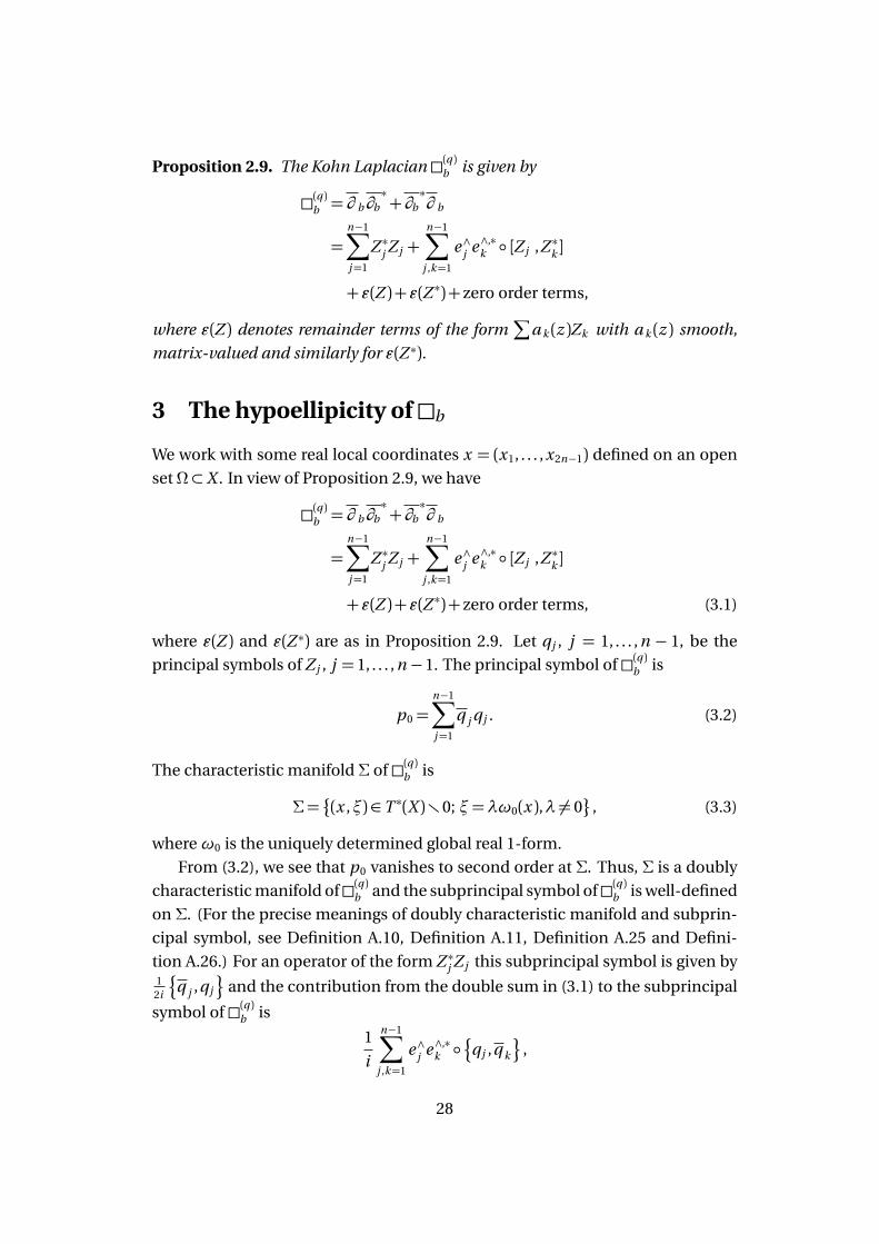
Proposition 2.9. The Kohn Laplacian (q )b is given by
(q )b = ∂ b∂b∗+ ∂b
∗∂ b
=n−1∑
j=1
Z ∗j Z j +n−1∑
j ,k=1
e ∧j e ∧,∗k [Z j ,Z ∗k ]
+ ε(Z )+ ε(Z ∗)+ zero order terms,
where ε(Z ) denotes remainder terms of the form∑
a k (z )Zk with a k (z ) smooth,
matrix-valued and similarly for ε(Z ∗).
3 The hypoellipicity ofb
We work with some real local coordinates x = (x1, . . . ,x2n−1) defined on an open
set Ω⊂X . In view of Proposition 2.9, we have
(q )b = ∂ b∂b∗+ ∂b
∗∂ b
=n−1∑
j=1
Z ∗j Z j +n−1∑
j ,k=1
e ∧j e ∧,∗k [Z j ,Z ∗k ]
+ ε(Z )+ ε(Z ∗)+ zero order terms, (3.1)
where ε(Z ) and ε(Z ∗) are as in Proposition 2.9. Let qj , j = 1, . . . , n − 1, be the
principal symbols of Z j , j = 1, . . . , n −1. The principal symbol of (q )b is
p0 =n−1∑
j=1
q j qj . (3.2)
The characteristic manifold Σ of (q )b is
Σ=
(x ,ξ)∈ T ∗(X )r0; ξ=λω0(x ),λ 6= 0
, (3.3)
whereω0 is the uniquely determined global real 1-form.
From (3.2), we see that p0 vanishes to second order at Σ. Thus, Σ is a doubly
characteristic manifold of(q )b and the subprincipal symbol of(q )b is well-defined
on Σ. (For the precise meanings of doubly characteristic manifold and subprin-
cipal symbol, see Definition A.10, Definition A.11, Definition A.25 and Defini-
tion A.26.) For an operator of the form Z ∗j Z j this subprincipal symbol is given by1
2i
¦
q j ,qj
©
and the contribution from the double sum in (3.1) to the subprincipal
symbol of (q )b is
1
i
n−1∑
j ,k=1
e ∧j e ∧,∗k
¦
qj ,q k
©
,
28
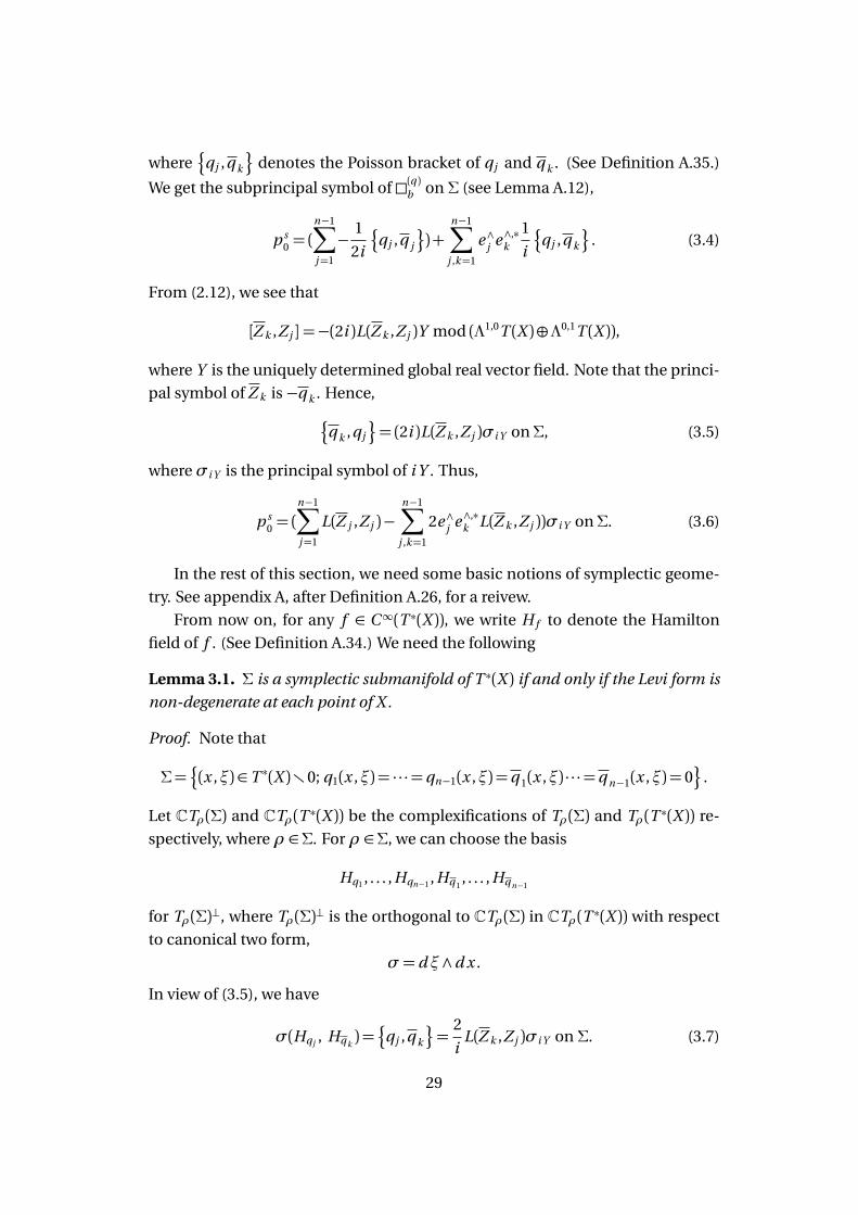
where¦
qj ,q k
©
denotes the Poisson bracket of qj and q k . (See Definition A.35.)
We get the subprincipal symbol of (q )b on Σ (see Lemma A.12),
p s0 = (
n−1∑
j=1
−1
2i
¦
qj ,q j
©
)+n−1∑
j ,k=1
e ∧j e ∧,∗k
1
i
¦
qj ,q k
©
. (3.4)
From (2.12), we see that
[Z k ,Z j ] =−(2i )L(Z k ,Z j )Y mod (Λ1,0T (X )⊕Λ0,1T (X )),
where Y is the uniquely determined global real vector field. Note that the princi-
pal symbol of Z k is −q k . Hence,
¦
q k ,qj
©
= (2i )L(Z k ,Z j )σi Y onΣ, (3.5)
whereσi Y is the principal symbol of i Y . Thus,
p s0 = (
n−1∑
j=1
L(Z j ,Z j )−n−1∑
j ,k=1
2e ∧j e ∧,∗k L(Z k ,Z j ))σi Y onΣ. (3.6)
In the rest of this section, we need some basic notions of symplectic geome-
try. See appendix A, after Definition A.26, for a reivew.
From now on, for any f ∈ C∞(T ∗(X )), we write H f to denote the Hamilton
field of f . (See Definition A.34.) We need the following
Lemma 3.1. Σ is a symplectic submanifold of T ∗(X ) if and only if the Levi form is
non-degenerate at each point of X .
Proof. Note that
Σ=¦
(x ,ξ)∈ T ∗(X )r0; q1(x ,ξ) = · · ·=qn−1(x ,ξ) =q 1(x ,ξ) · · ·=q n−1(x ,ξ) = 0©
.
Let CTρ(Σ) and CTρ(T ∗(X )) be the complexifications of Tρ(Σ) and Tρ(T ∗(X )) re-
spectively, where ρ ∈Σ. For ρ ∈Σ, we can choose the basis
Hq1 , . . . , Hqn−1 , Hq 1, . . . , Hq n−1
for Tρ(Σ)⊥, where Tρ(Σ)⊥ is the orthogonal to CTρ(Σ) in CTρ(T ∗(X )) with respect
to canonical two form,
σ= dξ∧d x .
In view of (3.5), we have
σ(Hqj , Hq k) =¦
qj ,q k
©
=2
iL(Z k ,Z j )σi Y on Σ. (3.7)
29
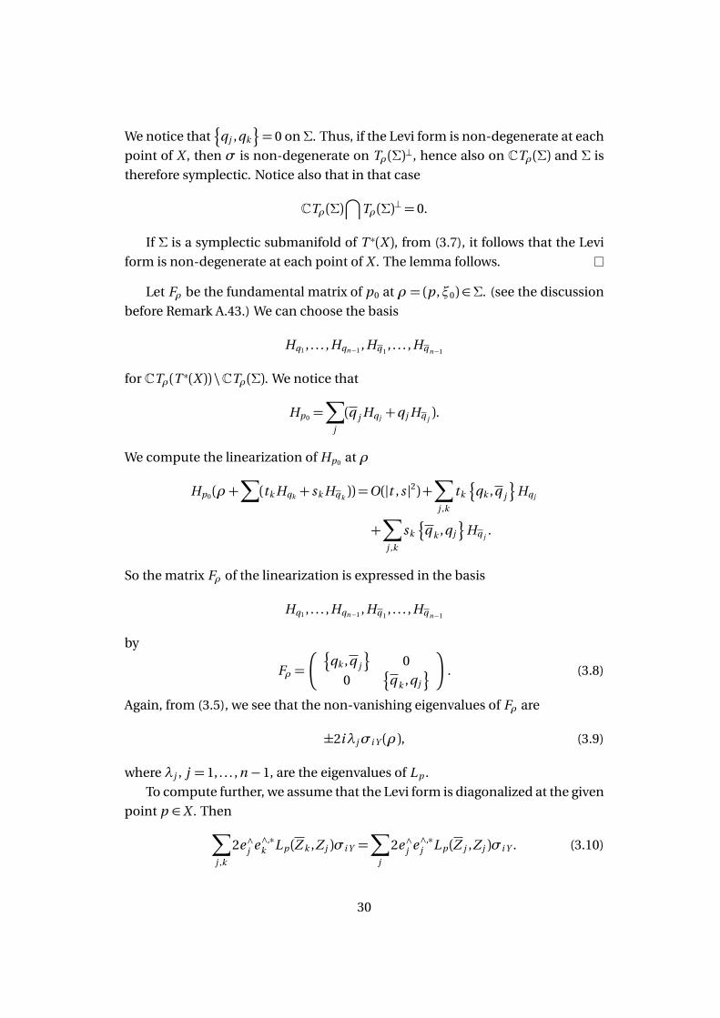
We notice that¦
qj ,qk
©
= 0 on Σ. Thus, if the Levi form is non-degenerate at each
point of X , then σ is non-degenerate on Tρ(Σ)⊥, hence also on CTρ(Σ) and Σ is
therefore symplectic. Notice also that in that case
CTρ(Σ)⋂
Tρ(Σ)⊥ = 0.
If Σ is a symplectic submanifold of T ∗(X ), from (3.7), it follows that the Levi
form is non-degenerate at each point of X . The lemma follows.
Let Fρ be the fundamental matrix of p0 at ρ = (p ,ξ0) ∈Σ. (see the discussion
before Remark A.43.) We can choose the basis
Hq1 , . . . , Hqn−1 , Hq 1, . . . , Hq n−1
for CTρ(T ∗(X )) \CTρ(Σ). We notice that
Hp0 =∑
j
(q j Hqj +qj Hq j).
We compute the linearization of Hp0 at ρ
Hp0(ρ+∑
(tk Hqk + sk Hq k)) =O(|t , s |2)+
∑
j ,k
tk
¦
qk ,q j
©
Hqj
+∑
j ,k
sk
¦
q k ,qj
©
Hq j.
So the matrix Fρ of the linearization is expressed in the basis
Hq1 , . . . , Hqn−1 , Hq 1, . . . , Hq n−1
by
Fρ =
¦
qk ,q j
©
0
0¦
q k ,qj
©
. (3.8)
Again, from (3.5), we see that the non-vanishing eigenvalues of Fρ are
±2iλjσi Y (ρ), (3.9)
where λj , j = 1, . . . , n −1, are the eigenvalues of L p .
To compute further, we assume that the Levi form is diagonalized at the given
point p ∈X . Then
∑
j ,k
2e ∧j e ∧,∗k L p (Z k ,Z j )σi Y =
∑
j
2e ∧j e ∧,∗j L p (Z j ,Z j )σi Y . (3.10)
30
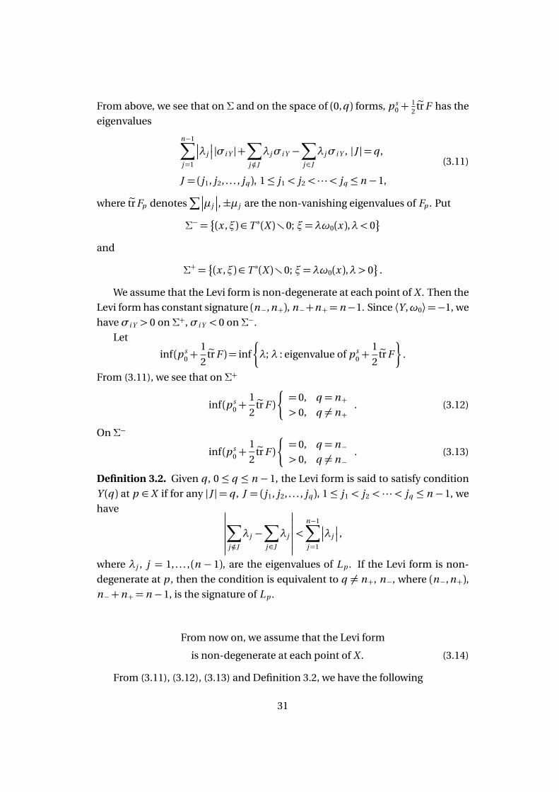
From above, we see that on Σ and on the space of (0,q ) forms, p s0 +
12etr F has the
eigenvalues
n−1∑
j=1
λj
|σi Y |+∑
j /∈J
λjσi Y −∑
j∈J
λjσi Y , |J |=q ,
J = (j1, j2, . . . , jq ), 1≤ j1 < j2 < · · ·< jq ≤ n −1,
(3.11)
where etr Fp denotes∑
µj
, ±µj are the non-vanishing eigenvalues of Fp . Put
Σ− =
(x ,ξ)∈ T ∗(X )r0; ξ=λω0(x ),λ< 0
and
Σ+ =
(x ,ξ)∈ T ∗(X )r0; ξ=λω0(x ),λ> 0
.
We assume that the Levi form is non-degenerate at each point of X . Then the
Levi form has constant signature (n−, n+), n−+n+ = n−1. Since ⟨Y ,ω0⟩=−1, we
haveσi Y > 0 on Σ+,σi Y < 0 on Σ−.
Let
inf (p s0 +
1
2etr F ) = inf
λ; λ : eigenvalue of p s0 +
1
2etr F
.
From (3.11), we see that on Σ+
inf (p s0 +
1
2etr F )
¨
= 0, q = n+> 0, q 6= n+
. (3.12)
On Σ−
inf (p s0 +
1
2etr F )
¨
= 0, q = n−> 0, q 6= n−
. (3.13)
Definition 3.2. Given q , 0 ≤ q ≤ n − 1, the Levi form is said to satisfy condition
Y (q ) at p ∈ X if for any |J |= q , J = (j1, j2, . . . , jq ), 1≤ j1 < j2 < · · ·< jq ≤ n − 1, we
have
∑
j /∈J
λj −∑
j∈J
λj
<n−1∑
j=1
λj
,
where λj , j = 1, . . . , (n − 1), are the eigenvalues of L p . If the Levi form is non-
degenerate at p , then the condition is equivalent to q 6= n+, n−, where (n−, n+),n−+n+ = n −1, is the signature of L p .
From now on, we assume that the Levi form
is non-degenerate at each point of X . (3.14)
From (3.11), (3.12), (3.13) and Definition 3.2, we have the following
31
Proposition 3.3. Let (n−, n+), n−+n+ = n − 1, be the signature of the Levi form
L. p s0 +
12etr F is positive semi-definite and we have that (3.12), (3.13) hold and
p s0 +
12etr F is positive definite when Y (q ) holds, precisely when q /∈ n+, n−.
Let Ω be an open set in RN . Let P be a classical pseudodifferential operator
on Ω of order m > 1. P is said to be hypoelliptic with loss of one derivative if
u ∈ E ′(Ω) and Pu ∈H sloc(Ω) implies u ∈H s+m−1
comp (Ω).We recall classical works by Boutet de Monvel [7] and Sjöstrand [21].
Proposition 3.4. Let Ω be an open set inRN . Let P be a classical pseudodifferential
operator on Ω of order m > 1. The symbol of P takes the form
σP (x ,ξ)∼ pm (x ,ξ)+pm−1(x ,ξ)+pm−2(x ,ξ)+ · · · ,
where p j is positively homogeneous of degree j . We assume that Σ = p−1m (0) is a
symplectic submanifold of codimension 2d , pm ≥ 0 and pm vanishes to precisely
second order on Σ. Let F be the fundamental matrix of pm . Let p sm be the subprin-
cipal symbol of P. Then P is hypoelliptic with loss of one derivative if and only
if
p sm (ρ)+
d∑
j=1
(1
2+αj )
µj
6= 0
at every point ρ ∈Σ for all (α1,α2, . . . ,αd ) ∈Nd , where ±iµj are the eigenvalues of
F at ρ.
Proposition 3.4 also holds if P is a matrix-valued classical pseudodifferential
operator on Ω of order m > 1 with scalar principal symbol.
From Proposition 3.4, we have the following
Proposition 3.5. We recall that we work with the assumption that the Levi form L
is non-degenerate at each point of X . (q )b is hypoelliptic with loss of one derivative
if and only if Y (q ) holds at each point of X .
Remark 3.6. Kohn’s L2 estimates give the hypoellipicity with loss of one dervative
for the solutions(q )b u = f under condition Y (q ). (See Folland-Kohn [11].) Kohn’s
method works as well when the Levi form L is degenerate.
4 The characteristic equation
In this section, we consider the characteristic equation for ∂t +(q )b .
Let p0(x ,ξ) be the principal symbol of (q )b . We work with some real local co-
ordinates x = (x1,x2, . . . ,x2n−1) defined on an open set Ω⊂ X . We identify Ω with
32
an open set inR2n−1. Let ΩC be an almost complexification of Ω. That is, ΩC is an
open set inC2n−1 withΩC⋂
R2n−1 =Ω. We identify T ∗(Ω)withΩ×R2n−1. Similarly,
let T ∗(Ω)C be an open set inC2n−1×C2n−1 with T ∗(Ω)C⋂
(R2n−1×R2n−1) = T ∗(Ω). In
this section, for any function f , we also write f to denote an almost analytic ex-
tension. (See Definition B.1.) We look for solutionsψ(t ,x ,η)∈C∞(R+×T ∗(Ω)\0)of the problem
∂ ψ
∂ t− i p0(x ,ψ′x ) =O(
Imψ
N), ∀N ≥ 0,
ψ|t=0 =
x ,η
(4.1)
with Imψ(t ,x ,η) ≥ 0. More precisely, we look for solutionsψ(t ,x ,η) ∈ C∞(R+×T ∗(Ω) \ 0) with Imψ(t ,x ,η) ≥ 0 such that ψ|t=0 =
x ,η
and for every compact
set K ⊂ T ∗(Ω) \0, N ≥ 0, there exists cK ,N ≥ 0, such that
∂ ψ
∂ t− i p0(x ,ψ′x )
≤ cK ,N
Imψ
Non R+×K .
Let f (x ,ξ), g (x ,ξ)∈C∞(T ∗(Ω)C). We write
f = g mod |Im (x ,ξ)|∞
if, given any compact subset K of T ∗(Ω)C and any integer N > 0, there is a con-
stant c > 0 such that
( f − g )(x ,ξ)
≤ c |Im (x ,ξ)|N , ∀(x ,ξ)∈ K .
Let U and V be C∞ complex vector fields on T ∗(Ω)C. We write
U =V mod |Im (x ,ξ)|∞
if
U ( f ) =V ( f )mod |Im (x ,ξ)|∞
and
U ( f ) =V ( f )mod |Im (x ,ξ)|∞ ,
for all almost analytic functions f on T ∗(Ω)C. In Appendix B, we discuss the no-
tions of almost analytic vector fields and equivalence of almost analytic vector
fields.
In the complex domain, the Hamiltonian field Hp0 is given by
Hp0 =∂ p0
∂ ξ
∂
∂ x−∂ p0
∂ x
∂
∂ ξ.
33
We notice that Hp0 depends on the choice of almost analytic extension of p0 but
we can give an invariant meaning of the exponential map exp(−i t Hp0), t ≥ 0.
Note that Hp0 vanishes on Σ. We consider the real vector field
−i Hp0 +−i Hp0 .
Let Φ(t ,ρ) be the −i Hp0 +−i Hp0 flow. We notice that for every T > 0 there is an
open neighborhood U of Σ in T ∗(Ω)C such that for all 0 ≤ t ≤ T , Φ(t ,ρ) is well-
defined if ρ ∈U . Since we only need to consider Taylor expansions at Σ, for the
convenience, we assume that Φ(t ,ρ) is well-defined for all t ≥ 0 and ρ ∈ T ∗(Ω)C.
We have the following
Proposition 4.1. Let Φ(t ,ρ) be as above. Let U be a real vector field on T ∗(Ω)Csuch that
U =−i Hp0 +−i Hp0 mod |Im (x ,ξ)|∞ .
Let Φ(t ,ρ) be the U flow. Then, for every compact set K ⊂ T ∗(Ω)C, N ≥ 0, there is
cN ,K (t )> 0, such that
Φ(t ,ρ)− Φ(t ,ρ)
≤ cN ,K (t )dist (ρ,Σ)N , ρ ∈ K .
Proof. This follows from Proposition B.13.
For t ≥ 0, let
G t =
(ρ,Φ(t ,ρ)); ρ ∈ T ∗(Ω)C
, (4.2)
whereΦ(t ,ρ) is as in Proposistion 4.1. We call G t the graph of exp (−i t Hp0). Since
Hp0 vanishes on Σ, we have
Φ(t ,ρ) =ρ if ρ ∈Σ.
G t depends on the choice of almost analytic extension of p0. Let p0 be another
almost analytic extension of p0. Let G t be the graph of exp (−i t Hp0). From Propo-
sition 4.1, it follows that G t coincides to infinite order with G t on diag (Σ×Σ), for
all t ≥ 0.
In Menikoff-Sjöstrand [20], it was shown that there exist g (t ,x ,η), h(t ,x ,η)∈C∞(R+×T ∗(Ω)C) such that
G t =
(x , g (t ,x ,η), h(t ,x ,η),η); (x ,η)∈ T ∗(Ω)C
.
Moreover, there existsψ(t ,x ,η)∈C∞(R+×T ∗(Ω)C) such that
g (t ,x ,η)−ψ′x (t ,x ,η)
34
and
h(t ,x ,η)−ψ′η(t ,x ,η)
vanish to infinite order on Σ, for all t ≥ 0. Furthermore, when (t ,x ,η) is real,
ψ(t ,x ,η) solves (4.1) and we have,
Imψ(t ,x ,η)t
1+ t(dist ((x ,η),Σ))2, t ≥ 0,
η
= 1. (4.3)
For the precise meaning of, see the discussion after Proposition 1.8. Moreover,
we have the following
Proposition 4.2. There exists ψ(t ,x ,η) ∈ C∞(R+ × T ∗(Ω) \ 0) such that Imψ ≥ 0
with equality precisely on (0 × T ∗(Ω) \ 0)⋃
(R+ × Σ) and such that (4.1) holds
where the error term is uniform on every set of the form [0, T ]×K with T > 0 and
K ⊂ T ∗(Ω)\0 compact. Furthermore,ψ is unique up to a term which is O(
Imψ
N)
locally uniformly for every N and
ψ(t ,x ,η) =
x ,η
onΣ, d x ,η(ψ−
x ,η
) = 0 onΣ.
Moreover, we have
Imψ(t ,x ,η)
η
t
η
1+ t
η
dist ((x ,η
η
),Σ))2, t ≥ 0,
η
≥ 1. (4.4)
Proposition 4.3. There exists a functionψ(∞,x ,η)∈C∞(T ∗(Ω)\0)with a uniquely
determined Taylor expansion at each point of Σ such that
For every compact set K ⊂ T ∗(Ω) \0 there is a constant cK > 0 such that
Imψ(∞,x ,η)≥ cK
η
(dist ((x ,η
η
),Σ))2,
d x ,η(ψ(∞,x ,η)−
x ,η
) = 0 on Σ.
If λ ∈C (T ∗(Ω) \ 0), λ > 0 and λ|Σ <min
λj
, where ±i
λj
are the non-vanishing
eigenvalues of the fundamental matrix of (q )b , then the solutionψ(t ,x ,η) of (4.1)
can be chosen so that for every compact set K ⊂ T ∗(Ω) \ 0 and all indices α, β , γ,
there is a constant cα,β ,γ,K such that
∂ αx ∂βη ∂
γt (ψ(t ,x ,η)−ψ(∞,x ,η))
≤ cα,β ,γ,K e−λ(x ,η)t onR+×K . (4.5)
For the proofs of Proposition 4.2 and Proposition 4.3, we refer the reader to
Menikoff-Sjöstrand [20]. From the positively homogeneity of p0, it follows that
35
we can chooseψ(t ,x ,η) in Proposition 4.2 to be quasi-homogeneous of degree 1
in the sense that
ψ(t ,x ,λη) =λψ(λt ,x ,η), λ> 0.
(See Definition 5.1.) This makesψ(∞,x ,η) positively homogeneous of degree 1.
We recall that
p0 =q1q 1+ · · ·+qn−1q n−1.
We can take an almost analytic extension of p0 so that
p0(x ,ξ) = p 0(x ,ξ). (4.6)
From (4.6), we have
−∂ ψ
∂ t(t ,x ,−η)− i p0(x ,ψ
′x (t ,x ,−η)) =O(
Imψ
N), t ≥ 0,
for all N ≥ 0, (x ,η) real. Since p0(x ,−ξ) = p0(x ,ξ), we have
−∂ ψ
∂ t(t ,x ,−η)− i p0(x ,−ψ
′x (t ,x ,−η)) =O(
Imψ
N), t ≥ 0, (4.7)
for all N ≥ 0, (x ,η) real. From Proposition 4.2, we can takeψ(t ,x ,η) so that
ψ(t ,x ,η) =−ψ(t ,x ,−η), (x ,η) is real. (4.8)
Hence,
ψ(∞,x ,η) =−ψ(∞,x ,−η), (x ,η) is real. (4.9)
PuteG t =
¦
(y ,η,x ,ξ); (x ,ξ, y ,η)∈G t
©
,
where G t is defined by (4.2). From (4.6), it follows that
Φ(t ,ρ) = Φ(−t ,ρ),
where Φ(t ,ρ) is as in Proposition 4.1. Thus, for all t ≥ 0,
G t = eG t . (4.10)
Put
C t =n
(x ,ψ′x (t ,x ,η),ψ′η(t ,x ,η),η); (x ,η)∈ T ∗(ΩC)o
(4.11)
andeC t =
¦
(y ,η,x ,ξ); (x ,ξ, y ,η)∈C t
©
. (4.12)
Since C t coincides to infinite order with G t on diag (Σ×Σ), for all t ≥ 0, from
(4.10), it follows that C t coincides to infinite order with eC t on diag (Σ×Σ), for all
t ≥ 0. Letting t →∞, we get the following
36
Proposition 4.4. Let
C∞ =n
(x ,ψ′x (∞,x ,η),ψ′η(∞,x ,η),η); (x ,η)∈ T ∗(ΩC)o
(4.13)
andeC∞ =
¦
(y ,η,x ,ξ); (x ,ξ, y ,η)∈C∞©
. (4.14)
Then eC∞ coincides to infinite order with C∞ on diag (Σ×Σ).
From Proposition 4.4 and the global theory of Fourier integral operators (see
Proposition B.21), we have the following
Proposition 4.5. The two phases
ψ(∞,x ,η)−
y ,η
∈C∞(Ω×Ω× R2n−1), −ψ(∞, y ,η)+
x ,η
∈C∞(Ω×Ω× R2n−1)
are equivalent in the sense of Definition B.20.
We recall that
Σ=¦
(x ,ξ)∈ T ∗(Ω)r0; q1(x ,ξ) = · · ·=qn−1(x ,ξ) =q 1(x ,ξ) · · ·=q n−1(x ,ξ) = 0©
.
For any function f ∈C∞(T ∗(Ω)), we use ef to denote an almost analytic extension
with respect to the weight function dist((x ,ξ),Σ). (See Definition B.1.) Set
eΣ=n
(x ,ξ)∈ T ∗(Ω)Cr0; eq1(x ,ξ) = · · ·= eqn−1(x ,ξ) = eq 1(x ,ξ) · · ·= eq n−1(x ,ξ) = 0o
.
(4.15)
We say that eΣ is an almost analytic extension with respect to the weight function
dist((x ,ξ),Σ) ofΣ. Let f (x ,ξ), g (x ,ξ)∈C∞(W ), where W is an open set in T ∗(Ω)C.
We write
f = g mod d∞Σ
if, given any compact subset K of W and any integer N > 0, there is a constant
c > 0 such that
( f − g )(x ,ξ)
≤ c dist ((x ,ξ),Σ)N , ∀(x ,ξ)∈ K .
From the global theory of Fourier integral operators (see Proposition B.21), we
only need to consider Taylor expansions at Σ. We may work with the following
coordinates
Proposition 4.6. Let ρ ∈ Σ. Then in some open neighborhood Γ of ρ in T ∗(Ω)C,
there are C∞ functions
ex j ∈C∞(Γ), eξj ∈C∞(Γ), j = 1, . . . , 2n −1,
such that
37
(a) ex j , eξj , j = 1, . . . , 2n − 1, are almost analytic functions with respect to the
weight function dist((x ,ξ),Σ).
(b)
det∂ (x ,ξ)
∂ (ex , eξ)
6= 0 on (Γ)R,
where (Γ)R =Γ⋂
T ∗(Ω) and ex = (ex1, . . . , ex2n−1), eξ= (eξ1, . . . , eξ2n−1).
(c) ex j , eξj , j = 1, . . . , 2n −1, form local coordinates of Γ.
(d) (ex , eξ) is symplectic to infinite order on Σ. That is,
ex j , exk = 0 mod d∞Σ , eξj , eξk = 0 mod d∞Σ ,
eξj , exk =δj ,k mod d∞Σ ,
where j , k = 1, . . . , 2n −1. Here
f , g
= ∂ f∂ ξ
∂ g∂ x− ∂ f∂ x∂ g∂ ξ
, f , g ∈C∞(Γ).
(e) We write ex ′, ex ′′, eξ′ and eξ′′ to denote (ex1, . . . , exn ), (exn+1, . . . , ex2n−1), (eξ1, . . . , eξn )and (eξn+1, . . . , eξ2n−1) respectively. Then, eΣ
⋂
Γ coincides to infinite order with
¦
(ex , eξ); ex ′′ = 0, eξ′′ = 0©
on Σ⋂
(Γ)R and
Σ⋂
(Γ)R =¦
(ex , eξ); ex ′′ = 0, eξ′′ = 0, ex ′ and eξ′ are real©
.
Furthermore, there is a (n−1)× (n−1)matrix of almost analytic functions A(ex , eξ)such that for every compact set K ⊂ Γ and N ≥ 0, there is a cK ,N > 0, such that
p0(ex , eξ)− i¬
A(ex , eξ)ex ′′, eξ′′¶
≤ cK ,N
(ex ′′, eξ′′)
N
on K ,
and when ex ′ and eξ′ are real, A(ex ′, 0, eξ′, 0) has only positive eigenvalues
|λ1| , . . . , |λn−1| ,
where±iλ1, . . . ,±iλn−1 are the non-vanishing eigenvalues of F (ex ′, 0, eξ′, 0), the fun-
damental matrix of (q )b . In particular,
1
2tr A(ex ′, 0, eξ′, 0) =
1
2etr F (ex ′, 0, eξ′, 0).
Formally, we write
p0(ex , eξ) = i¬
A(ex , eξ)ex ′′, eξ′′¶
+O(
(ex ′′, eξ′′)
N
). (4.16)
38
Proof. See Menikoff-Sjöstrand [20].
Remark 4.7. Set
E =¦
(t ,x ,ξ, y ,η)∈R+×T ∗(Ω)C×T ∗(Ω)C; (x ,ξ, y ,η)∈C t
©
,
where C t is defined by (4.11). Let (ex , eξ) be the coordinates of Proposition 4.6. In
the work of Menikoff-Sjöstrand [20], it was shown that there exists eψ(t , ex , eη) ∈C∞(R+×Γ), where Γ is as in Proposition 4.6, such that
∂ eψ
∂ t− i p0(ex , eψ′
ex ) =O(
(ex ′′, eη′′)
N), for all N > 0,
eψ|t=0 =
ex , eη
and eψ(t , ex , eη) is of the form
eψ(t , ex , eη) =
ex ′, eη′
+¬
e−t A(ex ′,0,eη′,0)ex ′′, eη′′
¶
+ eψ2(t , ex , eη)+ eψ3(t , ex , eη)+ · · · , (4.17)
where A is as in Proposition 4.6 and eψj (t , ex , eη) is a C∞ homogeneous polynomial
of degree j in (ex ′′, eη′′). If λ ∈ C (T ∗(Ω) \ 0), λ > 0 and λ|Σ < minλj with λj >
0, where ±iλj are the non-vanishing eigenvalues of the fundamental matrix of
(q )b , then for every compact set K ⊂ Σ⋂
(Γ)R and all indices α, β , γ, j , there is a
constant cα,β ,γ,j ,K such that
∂ αex ∂
βeη ∂
γt ( eψj (t , ex , eη))
≤ cα,β ,γ,K e−λ(ex ,eη)t onR+×K . (4.18)
Put
eE =
¨
(t , ex ,∂ eψ
∂ ex(t , ex , eη),
∂ eψ
∂ eη(t , ex , eη), eη); t ∈R+, ex , eη∈C∞(Γ)
«
.
We notice that eE coincides to infinite order with E on R+ × diag ((Σ⋂
(Γ)R) ×(Σ⋂
(Γ)R)). (See [20].)
5 The heat equation, formal construction
We work with some real local coordinates x = (x1, . . . ,x2n−1) defined on an open
set Ω⊂X . We identify T ∗(Ω)with Ω×R2n−1.
Definition 5.1. We will say that a ∈ C∞(R+ × T ∗(Ω)) is quasi-homogeneous of
degree j if a (t ,x ,λη) =λj a (λt ,x ,η) for all λ> 0.
39
It is easy to see that if a is quasi-homogeneous of degree j , then ∂ αx ∂βη ∂
γt a is
quasi-homogeneous of degree j −
β
+γ.
In this section, we consider the problem
¨
(∂t +(q )b )u (t ,x ) = 0 inR+×Ω
u (0,x ) = v (x ). (5.1)
We shall start by making only a formal construction. We look for an approximate
solution of (5.1) of the form
u (t ,x ) = A(t )v (x )
A(t )v (x ) =1
(2π)2n−1
∫ ∫
e i (ψ(t ,x ,η)−⟨y ,η⟩)a (t ,x ,η)v (y )d y dη (5.2)
where formally
a (t ,x ,η)∼∞∑
j=0
a j (t ,x ,η), a j (t ,x ,η)∈C∞(R+×T ∗(Ω);L (Λ0,q T ∗(Ω),Λ0,q T ∗(Ω))),
a j (t ,x ,η) is a quasi-homogeneous function of degree −j .
We let the full symbol of (q )b be:
full symbol of (q )b =2∑
j=0
p j (x ,ξ),
where p j (x ,ξ) is positively homogeneous of order 2− j . We apply ∂t +(q )b for-
mally under the integral in (5.2) and then introduce the asymptotic expansion
of(q )b (a e iψ). (See Proposition B.16.) Setting (∂t +(q )b )(a e iψ)∼ 0 and regrouping
the terms according to the degree of quasi-homogeneity. We obtain the transport
equations
(
T (t ,x ,η,∂t ,∂x )a 0 =O(
Imψ
N), ∀N
T (t ,x ,η,∂t ,∂x )a j + l j (t ,x ,η, a 0, . . . , a j−1) =O(
Imψ
N), ∀N .
(5.3)
Here
T (t ,x ,η,∂t ,∂x ) = ∂t − i2n−1∑
j=1
∂ p0
∂ ξj(x ,ψ′x )
∂
∂ x j+q (t ,x ,η)
where
q (t ,x ,η) = p1(x ,ψ′x )+1
2i
2n−1∑
j ,k=1
∂ 2p0(x ,ψ′x )∂ ξj ∂ ξk
∂ 2ψ(t ,x ,η)∂ x j ∂ xk
40
and l j is a linear differential operator acting on a 0, a 1, . . . , a j−1. We note that
q (t ,x ,η)→ q (∞,x ,η) exponentially fast in the sense of (4.5) and that the same
is true for the coefficients of l j .
Let C t , E be as in (4.11) and Remark 4.7. We recall that for t ≥ 0,
C t =
(x ,ξ, y ,η)∈ T ∗(Ω)C×T ∗(Ω)C; ξ=∂ ψ
∂ x(t ,x ,η), y =
∂ ψ
∂ η(t ,x ,η)
,
E =¦
(t ,x ,ξ, y ,η)∈R+×T ∗(Ω)C×T ∗(Ω)C; (x ,ξ, y ,η)∈C t
©
and for t > 0,
(C t )R = diag (Σ×Σ)=
(x ,ξ,x ,ξ)∈ T ∗(Ω)×T ∗(Ω); (x ,ξ)∈Σ
.
If we consider a 0, a 1, . . . as functions on E , then the equations (5.3) involve
differentiations along the vector field
ν =∂
∂ t− i Hp0 .
We can consider only Taylor expansions at Σ. Until further notice, our computa-
tions will only be valid to infinite order on Σ.
Consider ν as a vector field on E . In the coordinates (t ,x ,η) we can express
ν :
ν =∂
∂ t− i
2n−1∑
j=1
∂ p0
∂ ξj(x ,ψ′x )
∂
∂ x j.
We can compute
div (ν ) =1
i
2n−1∑
j=1
∂ 2p0(x ,ψ′x )∂ x j ∂ ξj
+2n−1∑
j ,k=1
∂ 2p0
∂ ξj ∂ ξk(x ,ψ′x )
∂ 2ψ
∂ x j ∂ xk(t ,x ,η)
. (5.4)
For a smooth function a (t ,x ,η)we introduce the 12
density on E
α= a (t ,x ,η)p
d t d x dη
which is well-defined up to some factor i µ. (See Hörmander [14].) The Lie deriva-
tive of α along ν is
Lν (α) = (ν (a )+1
2div (ν )a )
p
d t d x dη.
We see from the expression for T that
(Ta )p
d t d x dη= (Lν +p s0(x ,ψ′x (t ,x ,η)))(a
p
d t d x dη), (5.5)
41
where
p s0(x ,ξ) = p1(x ,ξ)+
i
2
2n−1∑
j=1
∂ 2p0(x ,ξ)∂ x j ∂ ξj
is the subprincipal symbol (invariantly defined on Σ). Now let (ex , eξ) be the coor-
dinates of Proposition 4.6, in which p0 takes the form (4.16). In these coordinates
we have
Hp0(ex , eξ) = i
A(ex , eξ)ex ′′ ,∂
∂ ex ′′
− i
®
tA(ex , eξ)eξ′′,∂
∂ eξ′′
¸
+∑
|α|=1,|β |=1
(ex ′′)α(eξ′′)βBαβ (ex , eξ,∂
∂ ex,∂
∂ eξ) (5.6)
and
ν =∂
∂ t+
A(ex , eψ′x )ex′′,∂
∂ ex ′′
+∑
|α|=1,|β |=1
(ex ′′)α( eψ′x ′′)βCαβ (ex ′, eψ′
ex ,∂
∂ ex). (5.7)
Here eψ(t , ex , eη) is as in Remark 4.7.
Let f (t ,x ,η)∈C∞(R+×T ∗(Ω)C), f (∞,x ,η)∈C∞(T ∗(Ω)C). We say that f (t ,x ,η)converges exponentially fast to f (∞,x ,η) if
f (t ,x ,η)− f (∞,x ,η)
satisfies the same kind of estimates as (4.5). Recalling the form of eψwe obtain
ν = ν =∂
∂ t+
A(ex ′, 0, eη′, 0)ex ′′,∂
∂ ex ′′
+∑
|α+β |=2,α 6=0
(ex ′′)α(eη′′)βDαβ (t , ex , eη,∂
∂ ex) (5.8)
where Dαβ converges exponentially fast to some limit as t →+∞. We have on Σ,
1
2div (ν ) =
1
2tr A(ex ′, 0, eη′, 0) =
1
2etr F (ex ′, 0, eη′, 0) (5.9)
where F (ex ′, 0, eη′, 0) is the fundamental matrix of (q )b . We define ea (t , ex , eη) by
ea (t , ex , eη)p
d t d ex d eη= a (t ,x ,η)p
d t d x dη. (5.10)
Note that the last equation only defines ea up to i µ. We have
(Ta )p
d t d x dη= ( eT ea )p
d t d ex d eη
42
where
eT =∂
∂ t+
A(ex ′, 0, eη′, 0)ex ′′,∂
∂ ex ′′
+1
2etr F (ex ′, 0, eη′, 0)+p s
0(ex′, 0, eη′, 0)+Q(t , ex , eη,
∂
∂ ex). (5.11)
Here
Q(t , ex , eη,∂
∂ ex) =
∑
|α+β |=2,α 6=0
(ex ′′)α(eη′′)βDαβ (t , ex , eη,∂
∂ ex)
+∑
|α+β |=1
(ex ′′)α(eη′′)βEαβ (t , ex , eη).
It is easy to see that Eαβ and Dαβ converge exponentially fast to some limits
Eαβ (∞, ex , eη) and Dαβ (∞, ex , eη) respectively. We need the following
Lemma 5.2. Let A be a d×d matrix having only positive eigenvalues and consider
the map
A : u 7→
*
A
x1
...
xd
,
∂ u∂ x1
...∂ u∂ xd
+
on the space Pm (Rd ) of homogeneous polynomials of degree m . Then
exp(tA )(u ) = u (exp(t A))
and the mapA is a bijection except for m = 0.
Proof. We notice that U (t ) : u 7→ u exp(t A) form a group of operators and that
(∂U (t )∂ t
)
t=0=A .
This shows that U (t ) = exp(tA ). To prove the second statement, suppose that
u ∈ Pm , m ≥ 1 and A (u ) = 0. Then exp(tA )(u ) = u for all t , in other words
u (exp(t A)(x )) = u (x ), t ∈ R, x ∈ Rd . Since exp(t A)(x ) → 0 when t → −∞, we
obtain u (x ) = u (0) = 0, which proves the lemma.
Proposition 5.3. Let
c j (x ,η)∈C∞(T ∗(Ω);L (Λ0,q T ∗(Ω),Λ0,q T ∗(Ω))), j = 0, 1, . . . ,
be positively homogeneous functions of degree −j . Then, we can find solutions
a j (t ,x ,η)∈C∞(R+×T ∗(Ω);L (Λ0,q T ∗(Ω),Λ0,q T ∗(Ω))), j = 0, 1, . . . ,
43
of the system (5.3) with
a j (0,x ,η) = c j (x ,η), j = 0, 1, . . . ,
where a j (t ,x ,η) is a quasi-homogeneous function of degree−j such that a j (t ,x ,η)has unique Taylor expansions on Σ, for all j . Furthermore, let λ(x ,η) ∈ C (T ∗(Ω))and λ|Σ < minτj , where τj are the eigenvalues of 1
2etr F + p s
0 on Σ. Then for all
indices α,β ,γ, j and every compact set K ⊂ Σ there exists a constant c > 0 such
that
∂γ
t ∂α
x ∂βη a j (t ,x ,η)
≤ c e−tλ(x ,η) onR+×K . (5.12)
Proof. We only need to study Taylor expansions on Σ. Let (ex , eξ) be the coordi-
nates of Proposition 4.6. We define ea j (t , ex , eη) from a j (t ,x ,η) as in (5.10). In or-
der to prove (5.12), it is sufficient to prove the corresponding statement for ea j .
(See section 1 of Menikoff-Sjöstrand[20].) We introduce the Taylor expansion of
ea 0 with respect to (ex ′′, eη′′).
ea 0(t , ex , eη) =∞∑
0
ea j0(t , ex , eη),
where ea j0 is a homogeneous polynomial of degree j in (ex ′′, eη′′). Let
c0(ex , eη) =∑
j=0
ec j0(ex , eη),
where ec j0 is a homogeneous polynomial of degree j in (ex ′′, eη′′). From eT ea 0 = 0, we
get
ea 00(t , ex ′, eη′) = e−t ( 1
2etr F+p s
0 )ec 0
0(ex , eη).
It is easy to see that for all indices α, β , γ and every compact set K ⊂ Σ there
exists a constant c > 0 such that
∂γ
t ∂αex ∂
βeη ea
00
≤ c e−tλ(ex ,eη) onR+×K ,
where λ(ex , eη) ∈ C (T ∗(Ω)), λ|Σ <minτj . Here τj are the eigenvalues of 12etr F +p s
0
on Σ.
Again, from eT ea 0 = 0, we get
(∂
∂ t+A +
1
2etr F +p s
0)eaj+10 (t , ex , eη) =eb j+1
0 (t , ex , eη)
where eb j+10 (t , ex , eη) satisfies the same kind of estimate as ea 0
0. By Lemma 5.2, we
see that exp(−tA ) is bounded for t ≥ 0. We deduce a similar estimate for the
44
function ea j+10 (t , ex , eη). Continuing in this way we get all the desired estimates for
ea 0. The next transport equation takes the form eT ea 1 = eb where eb satisfies the
estimates (5.12). We can repeat the procedure above and conclude that ea 1 satis-
fies the estimates (5.12). From above, we see that ea 0, ea 1 have the unique Taylor
expansions on Σ. Continuing in this way we get the proposition.
From Proposition 5.3, we have the following
Proposition 5.4. Suppose condition Y (q ) holds. Let
c j (x ,η)∈C∞(T ∗(Ω);L (Λ0,q T ∗(Ω),Λ0,q T ∗(Ω))), j = 0, 1, . . . ,
be positively homogeneous functions of degree −j . Then, we can find solutions
a j (t ,x ,η)∈C∞(R+×T ∗(Ω);L (Λ0,q T ∗(Ω),Λ0,q T ∗(Ω))), j = 0, 1, . . . ,
of the system (5.3) with
a j (0,x ,η) = c j (x ,η), j = 0, 1, . . . ,
where a j (t ,x ,η) is a quasi-homogeneous function of degree −j and ε0 > 0 such
that for all indices α,β ,γ, j and every compact set K ⊂ Ω there exists a constant
c > 0 such that
∂γ
t ∂α
x ∂βη a j (t ,x ,η)
≤ c e−ε0t |η|(1+
η
)−j−|β |+γ onR+×K . (5.13)
Proposition 5.5. Suppose condition Y (q ) fails. Let (n−, n+), n−+n+ = n − 1, be
the signature of the Levi form. Let
c j (x ,η)∈C∞(T ∗(Ω);L (Λ0,q T ∗(Ω),Λ0,q T ∗(Ω))), j = 0, 1, . . . ,
be positively homogeneous functions of degree −j . Then, we can find solutions
a j (t ,x ,η)∈C∞(R+×T ∗(Ω);L (Λ0,q T ∗(Ω),Λ0,q T ∗(Ω))), j = 0, 1, . . . ,
of the system (5.3) with
a j (0,x ,η) = c j (x ,η), j = 0, 1, . . . ,
where a j (t ,x ,η) is a quasi-homogeneous function of degree −j and such that for
all indices α,β ,γ, j , every ε > 0 and compact set K ⊂Σ there exists a constant c > 0
such that
∂γ
t ∂α
x ∂βη a j (t ,x ,η)
≤ c e εt |η|(1+
η
)−j−|β |+γ onR+×K . (5.14)
45
Furthermore, there exists ε0 > 0 such that for all indices α,β ,γ, j and every com-
pact set K ⊂Σ, there exists a constant c > 0 such that
∂γ
t ∂α
x ∂βη a j (t ,x ,η)
≤ c e−ε0t |η|(1+
η
)−j−|β |+γ
onR+× (K⋂
Σ+) if q = n−, n− 6= n+ (5.15)
and
∂γ
t ∂α
x ∂βη a j (t ,x ,η)
≤ c e−ε0t |η|(1+
η
)−j−|β |+γ
onR+× (K⋂
Σ−) if q = n+, n− 6= n+. (5.16)
We need the following formula
Proposition 5.6. Let Q be a C∞ differential operator on Ω of order k > 0 with full
symbol q (x ,ξ)∈C∞(T ∗(Ω)). For 0≤q ,q1 ≤ n −1, q , q1 ∈N, let
a (t ,x ,η)∈C∞(R+×T ∗(Ω);L (Λ0,q1 T ∗(Ω),Λ0,q T ∗(Ω))).
Then,
Q(x , Dx )(e iψ(t ,x ,η)a (t ,x ,η)) = e iψ(t ,x ,η)∑
|α|≤k
1
α!q (α)(x ,ψ′x (t ,x ,η))(Rα(ψ, Dx )a ),
where
Dx =−i∂x ,
Rα(ψ, Dx )a =Dαy
¦
e iφ2(t ,x ,y ,η)a (t , y ,η)©
y=x,
φ2(t ,x , y ,η) = (x − y )ψ′x (t ,x ,η)− (ψ(t ,x ,η)−ψ(t , y ,η)).
For 0≤q ,q1 ≤ n −1, q , q1 ∈N, let
a j (t ,x ,η)∈C∞(R+×T ∗(Ω);L (Λ0,q1 T ∗(Ω),Λ0,q T ∗(Ω))), j = 0, 1, . . . , (5.17)
be quasi-homogeneous functions of degree m − j , m ∈Z. We assume that
a j (t ,x ,η), j = 0, 1, . . . ,
are the solutions of the system (5.3). From the proof of Proposition 5.3, it follows
that for all indices α,β ,γ, j , every ε > 0 and compact set K ⊂ Σ there exists a
constant c > 0 such that
∂γ
t ∂α
x ∂βη a j (t ,x ,η)
≤ c e εt |η|(1+
η
)m−j−|β |+γ onR+×K . (5.18)
46
Let
a (t ,x ,η)∈C∞(R+×T ∗(Ω);L (Λ0,q1 T ∗(Ω),Λ0,q T ∗(Ω))) (5.19)
be the asymptotic sum of a j (t ,x ,η). (See Definition 6.1 and Remark 6.2 for a
precise meaning.) We formally write
a (t ,x ,η)∼∞∑
j=0
a j (t ,x ,η).
Let
(∂t +(q )b )(e
iψ(t ,x ,η)a (t ,x ,η)) = e iψ(t ,x ,η)b (t ,x ,η),
where
b (t ,x ,η)∼∞∑
j=0
b j (t ,x ,η),
b j (t ,x ,η)∈C∞(R+×T ∗(Ω);L (Λ0,q1 T ∗(Ω),Λ0,q T ∗(Ω))), j = 0, 1, . . . ,
b j (t ,x ,η) is a quasi-homogeneous function of degree m +2− j .
From Proposition 5.6, we see that for all N , every compact set K ⊂ Σ, ε > 0,
there exists c > 0 such that
b (t ,x ,η)
≤ c e εt |η|(
η
−N+
η
2−N(Imψ(t ,x ,η)N ) (5.20)
on R+×K ,
η
≥ 1.
Conversely, if
(∂t +(q )b )(e
iψ(t ,x ,η)a (t ,x ,η)) = e iψ(t ,x ,η)b (t ,x ,η)
and b satisfies the same kind of estimates as (5.20), then a j (t ,x ,η), j = 0, 1, . . .,
solve the system (5.3) to infinite order atΣ. From this and the particular structure
of the problem, we will next show
Proposition 5.7. Let (n−, n+), n−+n+ = n − 1, be the signature of the Levi form.
Suppose condition Y (q ) fails. That is, q = n− or n+. Let
a j (t ,x ,η)∈C∞(R+×T ∗(Ω);L (Λ0,q T ∗(Ω),Λ0,q T ∗(Ω))), j = 0, 1, . . . ,
be the solutions of the system (5.3) with
a 0(0,x ,η) = I , a j (0,x ,η) = 0 when j > 0,
where a j (t ,x ,η) is a quasi-homogeneous function of degree −j . Then we can find
a j (∞,x ,η)∈C∞(T ∗(Ω);L (Λ0,q T ∗(Ω),Λ0,q T ∗(Ω))), j = 0, 1, . . . ,
47
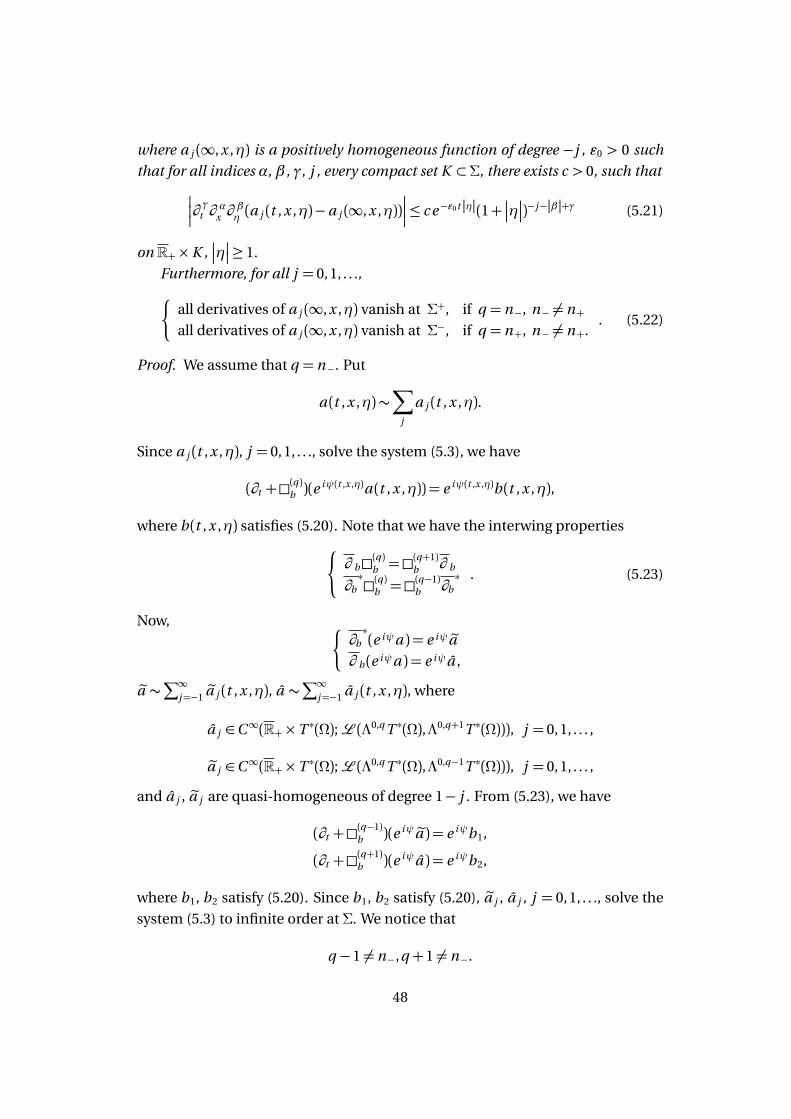
where a j (∞,x ,η) is a positively homogeneous function of degree −j , ε0 > 0 such
that for all indices α, β , γ, j , every compact set K ⊂Σ, there exists c > 0, such that
∂γ
t ∂α
x ∂βη (a j (t ,x ,η)−a j (∞,x ,η))
≤ c e−ε0t |η|(1+
η
)−j−|β |+γ (5.21)
on R+×K ,
η
≥ 1.
Furthermore, for all j = 0, 1, . . .,
¨
all derivatives of a j (∞,x ,η) vanish at Σ+, if q = n−, n− 6= n+all derivatives of a j (∞,x ,η) vanish at Σ−, if q = n+, n− 6= n+.
. (5.22)
Proof. We assume that q = n−. Put
a (t ,x ,η)∼∑
j
a j (t ,x ,η).
Since a j (t ,x ,η), j = 0, 1, . . ., solve the system (5.3), we have
(∂t +(q )b )(e
iψ(t ,x ,η)a (t ,x ,η)) = e iψ(t ,x ,η)b (t ,x ,η),
where b (t ,x ,η) satisfies (5.20). Note that we have the interwing properties
(
∂ b(q )b =
(q+1)b ∂ b
∂b∗(q )b =
(q−1)b ∂b
∗ . (5.23)
Now,¨
∂b∗(e iψa ) = e iψ
ea
∂ b (e iψa ) = e iψa ,
ea ∼∑∞
j=−1 ea j (t ,x ,η), a ∼∑∞
j=−1 a j (t ,x ,η), where
a j ∈C∞(R+×T ∗(Ω);L (Λ0,q T ∗(Ω),Λ0,q+1T ∗(Ω))), j = 0, 1, . . . ,
ea j ∈C∞(R+×T ∗(Ω);L (Λ0,q T ∗(Ω),Λ0,q−1T ∗(Ω))), j = 0, 1, . . . ,
and a j , ea j are quasi-homogeneous of degree 1− j . From (5.23), we have
(∂t +(q−1)b )(e iψ
ea ) = e iψb1,
(∂t +(q+1)b )(e iψa ) = e iψb2,
where b1, b2 satisfy (5.20). Since b1, b2 satisfy (5.20), ea j , a j , j = 0, 1, . . ., solve the
system (5.3) to infinite order at Σ. We notice that
q −1 6= n−,q +1 6= n−.
48
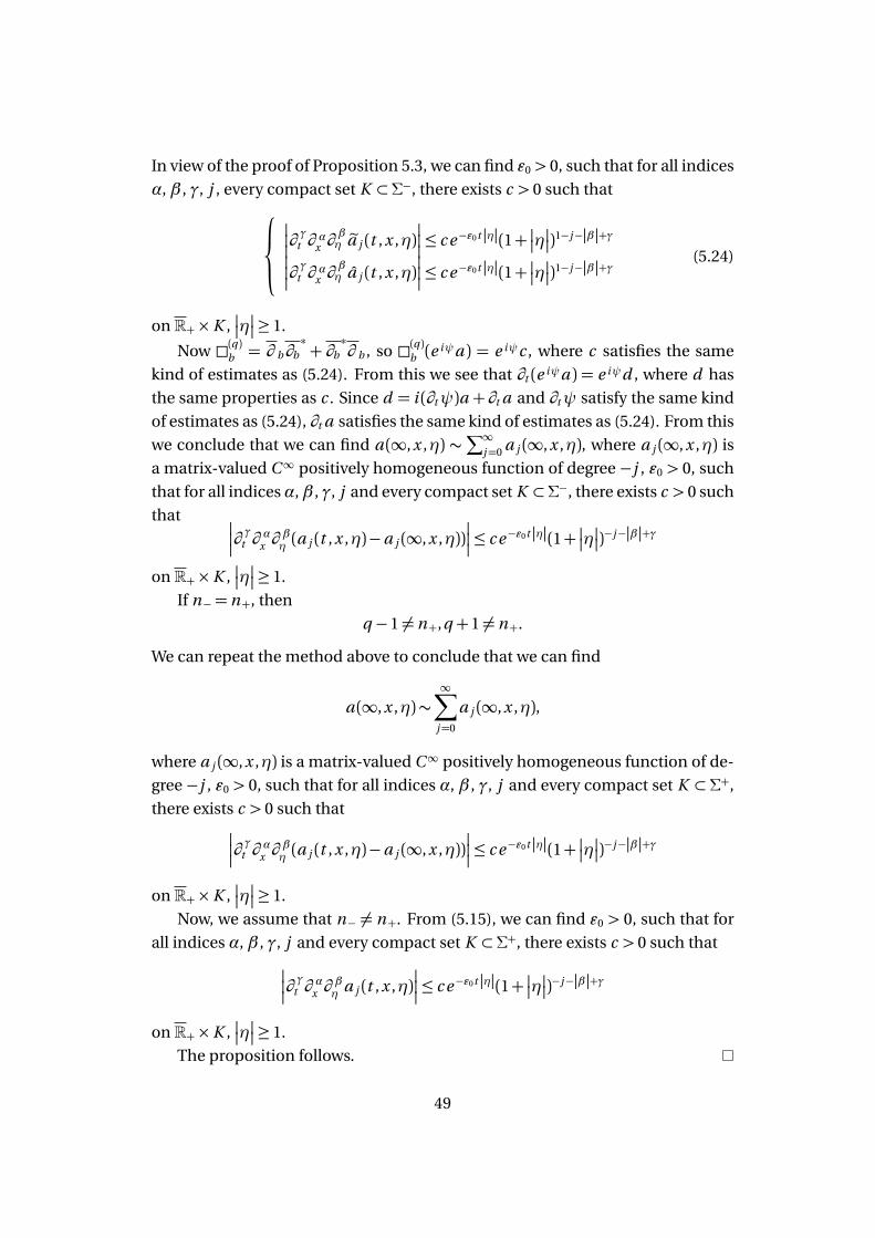
In view of the proof of Proposition 5.3, we can find ε0 > 0, such that for all indices
α, β , γ, j , every compact set K ⊂Σ−, there exists c > 0 such that
∂γ
t ∂α
x ∂βη ea j (t ,x ,η)
≤ c e−ε0t |η|(1+
η
)1−j−|β |+γ
∂γ
t ∂α
x ∂βη a j (t ,x ,η)
≤ c e−ε0t |η|(1+
η
)1−j−|β |+γ (5.24)
on R+×K ,
η
≥ 1.
Now (q )b = ∂ b∂b∗+ ∂b
∗∂ b , so (q )b (e
iψa ) = e iψc , where c satisfies the same
kind of estimates as (5.24). From this we see that ∂t (e iψa ) = e iψd , where d has
the same properties as c . Since d = i (∂tψ)a + ∂t a and ∂tψ satisfy the same kind
of estimates as (5.24), ∂t a satisfies the same kind of estimates as (5.24). From this
we conclude that we can find a (∞,x ,η) ∼∑∞
j=0 a j (∞,x ,η), where a j (∞,x ,η) is
a matrix-valued C∞ positively homogeneous function of degree −j , ε0 > 0, such
that for all indicesα, β , γ, j and every compact set K ⊂Σ−, there exists c > 0 such
that
∂γ
t ∂α
x ∂βη (a j (t ,x ,η)−a j (∞,x ,η))
≤ c e−ε0t |η|(1+
η
)−j−|β |+γ
on R+×K ,
η
≥ 1.
If n− = n+, then
q −1 6= n+,q +1 6= n+.
We can repeat the method above to conclude that we can find
a (∞,x ,η)∼∞∑
j=0
a j (∞,x ,η),
where a j (∞,x ,η) is a matrix-valued C∞ positively homogeneous function of de-
gree −j , ε0 > 0, such that for all indices α, β , γ, j and every compact set K ⊂Σ+,
there exists c > 0 such that
∂γ
t ∂α
x ∂βη (a j (t ,x ,η)−a j (∞,x ,η))
≤ c e−ε0t |η|(1+
η
)−j−|β |+γ
on R+×K ,
η
≥ 1.
Now, we assume that n− 6= n+. From (5.15), we can find ε0 > 0, such that for
all indices α, β , γ, j and every compact set K ⊂Σ+, there exists c > 0 such that
∂γ
t ∂α
x ∂βη a j (t ,x ,η)
≤ c e−ε0t |η|(1+
η
)−j−|β |+γ
on R+×K ,
η
≥ 1.
The proposition follows.
49
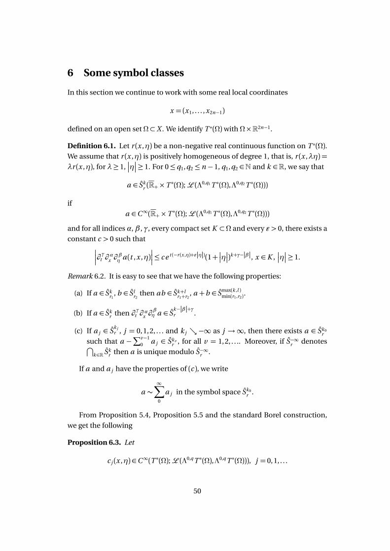
6 Some symbol classes
In this section we continue to work with some real local coordinates
x = (x1, . . . ,x2n−1)
defined on an open set Ω⊂X . We identify T ∗(Ω)with Ω×R2n−1.
Definition 6.1. Let r (x ,η) be a non-negative real continuous function on T ∗(Ω).We assume that r (x ,η) is positively homogeneous of degree 1, that is, r (x ,λη) =λr (x ,η), for λ≥ 1,
η
≥ 1. For 0≤q1,q2 ≤ n −1, q1,q2 ∈N and k ∈R, we say that
a ∈ Skr (R+×T ∗(Ω);L (Λ0,q1 T ∗(Ω),Λ0,q2 T ∗(Ω)))
if
a ∈C∞(R+×T ∗(Ω);L (Λ0,q1 T ∗(Ω),Λ0,q2 T ∗(Ω)))
and for all indices α, β , γ, every compact set K ⊂Ω and every ε > 0, there exists a
constant c > 0 such that
∂γ
t ∂α
x ∂βη a (t ,x ,η)
≤ c e t (−r (x ,η)+ε|η|)(1+
η
)k+γ−|β |, x ∈ K ,
η
≥ 1.
Remark 6.2. It is easy to see that we have the following properties:
(a) If a ∈ Skr1
, b ∈ Slr2
then ab ∈ Sk+lr1+r2
, a +b ∈ Smax(k ,l )min(r1,r2)
.
(b) If a ∈ Skr then ∂ γt ∂ αx ∂
βη a ∈ S
k−|β |+γr .
(c) If a j ∈ Sk jr , j = 0, 1, 2, . . . and k j −∞ as j →∞, then there exists a ∈ Sk0
r
such that a −∑v−1
0 a j ∈ Skvr , for all v = 1, 2, . . .. Moreover, if S−∞r denotes
⋂
k∈R Skr then a is unique modulo S−∞r .
If a and a j have the properties of (c ), we write
a ∼∞∑
0
a j in the symbol space Sk0r .
From Proposition 5.4, Proposition 5.5 and the standard Borel construction,
we get the following
Proposition 6.3. Let
c j (x ,η)∈C∞(T ∗(Ω);L (Λ0,q T ∗(Ω),Λ0,q T ∗(Ω))), j = 0, 1, . . .
50
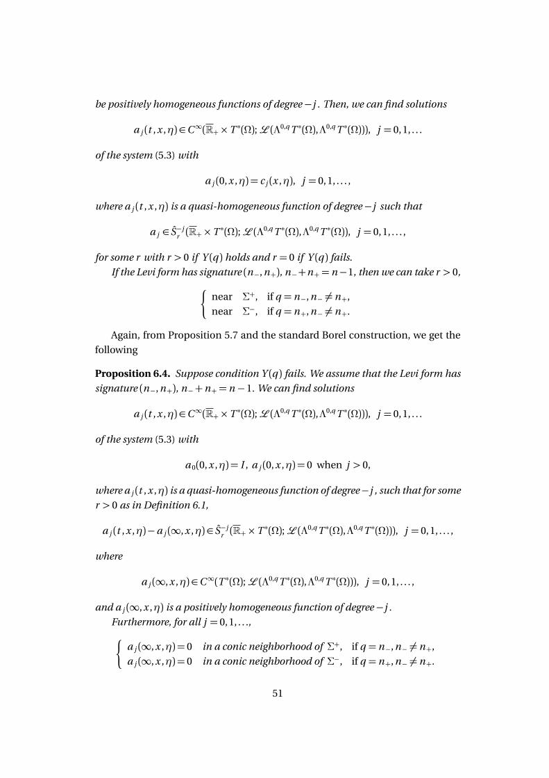
be positively homogeneous functions of degree −j . Then, we can find solutions
a j (t ,x ,η)∈C∞(R+×T ∗(Ω);L (Λ0,q T ∗(Ω),Λ0,q T ∗(Ω))), j = 0, 1, . . .
of the system (5.3) with
a j (0,x ,η) = c j (x ,η), j = 0, 1, . . . ,
where a j (t ,x ,η) is a quasi-homogeneous function of degree −j such that
a j ∈ S−jr (R+×T ∗(Ω);L (Λ0,q T ∗(Ω),Λ0,q T ∗(Ω)), j = 0, 1, . . . ,
for some r with r > 0 if Y (q ) holds and r = 0 if Y (q ) fails.
If the Levi form has signature (n−, n+), n−+n+ = n−1, then we can take r > 0,
¨
near Σ+, if q = n−, n− 6= n+,
near Σ−, if q = n+, n− 6= n+.
Again, from Proposition 5.7 and the standard Borel construction, we get the
following
Proposition 6.4. Suppose condition Y (q ) fails. We assume that the Levi form has
signature (n−, n+), n−+n+ = n −1. We can find solutions
a j (t ,x ,η)∈C∞(R+×T ∗(Ω);L (Λ0,q T ∗(Ω),Λ0,q T ∗(Ω))), j = 0, 1, . . .
of the system (5.3) with
a 0(0,x ,η) = I , a j (0,x ,η) = 0 when j > 0,
where a j (t ,x ,η) is a quasi-homogeneous function of degree−j , such that for some
r > 0 as in Definition 6.1,
a j (t ,x ,η)−a j (∞,x ,η)∈ S−jr (R+×T ∗(Ω);L (Λ0,q T ∗(Ω),Λ0,q T ∗(Ω))), j = 0, 1, . . . ,
where
a j (∞,x ,η)∈C∞(T ∗(Ω);L (Λ0,q T ∗(Ω),Λ0,q T ∗(Ω))), j = 0, 1, . . . ,
and a j (∞,x ,η) is a positively homogeneous function of degree −j .
Furthermore, for all j = 0, 1, . . .,
¨
a j (∞,x ,η) = 0 in a conic neighborhood of Σ+, if q = n−, n− 6= n+,
a j (∞,x ,η) = 0 in a conic neighborhood of Σ−, if q = n+, n− 6= n+.
51
Let b (t ,x ,η)∈ Skr , r > 0. Our next goal is to define the operator
B (t ,x , y ) =
∫
e i (ψ(t ,x ,η)−⟨y ,η⟩)b (t ,x ,η)dη
as an oscillatory integral. We have the following
Proposition 6.5. Let
b (t ,x ,η)∈ Skr (R+×T ∗(Ω);L (Λ0,q1 T ∗(Ω),Λ0,q2 T ∗(Ω)))
with r > 0. Then we can define
B (t ) : C∞0 (Ω; Λ0,q1 T ∗(Ω))→C∞(R+; C∞(Ω; Λ0,q2 T ∗(Ω)))
with distribution kernel
B (t ,x , y ) =
∫
e i (ψ(t ,x ,η)−⟨y ,η⟩)b (t ,x ,η)dη
and B (t ) has a unique continuous extension
B (t ) : E ′(Ω; Λ0,q1 T ∗(Ω))→C∞(R+;D ′(Ω; Λ0,q2 T ∗(Ω))).
We have
B (t ,x , y )∈C∞(R+; C∞(Ω×Ωrdiag (Ω×Ω);L (Λ0,q1 T ∗(Ω),Λ0,q2 T ∗(Ω)))),
and
B (t ,x , y )|t>0 ∈C∞(R+×Ω×Ω;L (Λ0,q1 T ∗(Ω),Λ0,q2 T ∗(Ω))).
Proof. Let
S∗Ω=¦
(x ,η)∈Ω× R2n−1;
η
= 1©
,
and let
V ⊂R+×S∗Ω
be a neighborhood of
(R+× (Σ⋂
S∗Ω))⋃
(0×S∗Ω)
such that
Vt =
(x ,η); (t ,x ,η)∈V
is independent of t for large t . Set
W =
(
(t ,x ,η)∈R+×Ω× R2n−1; (
η
t ,x ,η
η
)∈V
)
.
52
Let χV ∈C∞(R+×S∗(Ω)) have its support in V , be equal to 1 in a neighborhood of
(R+×S∗Σ)⋃
(0×S∗Ω), and be independent of t , for large t . Set
χW (t ,x ,η) =χV (
η
t ,x ,η
η
)∈C∞(R+×Ω× R2n−1).
We have χW (t ,x ,λη) =χW (λt ,x ,η), λ> 0. We can choose V sufficiently small so
that
ψ′x (t ,x ,η)−η
≤
η
2in W. (6.1)
We formally set
B (t ,x , y ) =
∫
e i (ψ(t ,x ,η)−⟨y ,η⟩)(1−χW (t ,x ,η))b (t ,x ,η)dη
+
∫
e i (ψ(t ,x ,η)−⟨y ,η⟩)χW (t ,x ,η)b (t ,x ,η)dη
= B1(t ,x , y )+ B2(t ,x , y )
where in B1(t ,x , y ) and B2(t ,x , y ) we have introduced the cut-off functions (1−χW ) and χW respectively. Choose χ ∈ C∞0 (R2n−1) so that χ(η) = 1 when
η
< 1
and χ(η) = 0 when
η
> 2. Since Imψ > 0 outside (R+ ×Σ)⋃
(0 × R2n−1), we
have
Imψ(t ,x ,η)≥ c
η
outside W,
where c > 0. The kernel
B1,ε(t ,x , y ) =
∫
e i (ψ(t ,x ,η)−⟨y ,η⟩)(1−χW (t ,x ,η))b (t ,x ,η)χ(εη)dη
converges in C∞(R+×Ω×Ω;L (Λ0,q1 T ∗(Ω),Λ0,q2 T ∗(Ω))) as ε→ 0. This means that
B1(t ,x , y ) = limε→0
B1,ε(t ,x , y )∈C∞(R+×Ω×Ω;L (Λ0,q1 T ∗(Ω),Λ0,q2 T ∗(Ω))).
To study B2(t ,x , y ) take a u (y )∈C∞0 (K ; Λ0,q1 T ∗(Ω)), K ⊂⊂Ω and set
χν (η) =χ(2−νη)−χ(21−νη), ν > 0, χ0(η) =χ(η).
Then we have∞∑
ν=0
χν = 1 and 2ν−1 ≤
η
≤ 2ν+1 whenη∈ suppχν , ν 6= 0.
We assume that b (t ,x ,η) = 0 if
η
≤ 1. If x ∈ K , we obtain for all indices α, β and
every ε > 0, there exists cε,α,β ,K > 0, such that
Dαx Dβ
η (χν (η)χW (t ,x ,η)b (t ,x ,η))
≤ cε,α,β ,K e t (−r (x ,η)+ε|η|)(1+
η
)k−|β |. (6.2)
53
Note that
Dαχν (η)
≤ cα(1+
η
)−|α| with a constant independent of ν . We have
B2,ν+1 =
∫ ∫
e i (ψ(t ,x ,η)−⟨y ,η⟩)χν+1(η)χW (t ,x ,η)b (t ,x ,η)u (y )d y dη
= 2(2n−1)ν
∫
e iλ(ψ(λt ,x ,η)−⟨y ,η⟩)χ1(η)χW (t ,x ,λη)b (t ,x ,λη)u (y )d y dη,
where λ= 2ν . Since (6.2) holds, we have
Dαη(χW (t ,x , 2νη)b (t ,x , 2νη))
≤ c 2kν ,
if x ∈ K , 1 <
η
< 4, where c > 0. Since d y (ψ(λt ,x ,η)−
y ,η
) 6= 0, if η 6= 0, we
can integrate by parts and obtain
B2,ν+1
≤ c 2ν (2n−1+k−m )∑
|α|≤m
sup |Dαu | .
Since m can be chosen arbitrary large, we conclude that∑
ν
B2,ν
: converges
and that B (t ) defines an operator
B (t ) : C∞0 (Ωy ; Λ0,q1 T ∗(Ω))→C∞(R+×Ωx ; Λ0,q2 T ∗(Ω)).
Let B ∗(t ) be the formal adjoint of B (t )with respect to ( | ). From (6.1), we see that
ψ′x (t ,x ,η) 6= 0 on W . We can repeat the procedure above and conclude that B ∗(t )defines an operator
C∞0 (Ωx ; Λ0,q2 T ∗(Ω))→C∞(R+×Ωy ; Λ0,q1 T ∗(Ω)).
Hence, we can extend B (t ) to
E ′(Ω; Λ0,q1 T ∗(Ω))→C∞(R+;D ′(Ω; Λ0,q2 T ∗(Ω)))
by the following formula
(B (t )u (y ) | v (x )) = (u (y ) | B ∗(t )v (x )), u ∈ E ′(Ω; Λ0,q1 T ∗(Ω)), v ∈C∞0 (Ω; Λ0,q2 T ∗(Ω)).
When x 6= y and (x , y ) ∈ Σ×Σ, we have dη(ψ(t ,x ,η)−
y ,η
) 6= 0, we can
repeat the procedure above and conclude that
B (t ,x , y )∈C∞(R+; C∞(Ω×Ωrdiag (Ω×Ω);L (Λ0,q1 T ∗(Ω),Λ0,q2 T ∗(Ω)))).
Finally, in view of the exponential decrease as t →∞ of the symbol b (t ,x ,η),we see that the kernel B (t )|t>0 is smoothing.
54
Let b (t ,x ,η) ∈ Skr with r > 0. Our next step is to show that we can also define
the operator
B (x , y ) =
∫
∫ ∞
0
e i (ψ(t ,x ,η)−⟨y ,η⟩)b (t ,x ,η)d t
dη
as an oscillatory integral. We have the following
Proposition 6.6. Let
b (t ,x ,η)∈ Skr (R+×T ∗(Ω);L (Λ0,q1 T ∗(Ω),Λ0,q2 T ∗(Ω)))
with r > 0. We assume that b (t ,x ,η) = 0 when
η
≤ 1. Then we can define
B : C∞0 (Ω; Λ0,q1 T ∗(Ω))→C∞(Ω; Λ0,q2 T ∗(Ω))
with distribution kernel
B (x , y ) =1
(2π)2n−1
∫
∫ ∞
0
e i (ψ(t ,x ,η)−⟨y ,η⟩)b (t ,x ,η)d t
dη
and B has a unique continuous extension
B : E ′(Ω; Λ0,q1 T ∗(Ω))→D ′(Ω; Λ0,q2 T ∗(Ω)).
Moreover, we have
B (x , y )∈C∞(Ω×Ωrdiag (Ω×Ω);L (Λ0,q1 T ∗(Ω),Λ0,q2 T ∗(Ω))).
Proof. Let W and χW (t ,x ,η) be as in Proposition 6.5. We formally set
B (x , y ) =1
(2π)2n−1
∫ ∫ ∞
0
e i (ψ(t ,x ,η)−⟨y ,η⟩)(1−χW (t ,x ,η))b (t ,x ,η)d t dη
+1
(2π)2n−1
∫ ∫ ∞
0
e i (ψ(t ,x ,η)−⟨y ,η⟩)χW (t ,x ,η)b (t ,x ,η)d t dη
= B1(x , y )+ B2(x , y )
where in B1(x , y ) and B2(x , y ) we have introduced the cut-off functions (1−χW )and χW respectively. Since
Imψ(t ,x ,η)≥ c ′
η
outside W,
where c ′ > 0, we have
e i (ψ(t ,x ,η)−⟨y ,η⟩)(1−χW (t ,x ,η))b (t ,x ,η)
≤ c e−c ′|η|e−ε0t |η|(1+
η
)k , ε0 > 0
55
and similar estimates for the derivatives. From this, we see that B1(x , y )∈C∞(Ω×Ω;L (Λ0,q1 T ∗(Ω),Λ0,q2 T ∗(Ω))).
Choose χ ∈ C∞0 (R2n−1) so that χ(η) = 1 when
η
< 1 and χ(η) = 0 when
η
> 2. To study B2(x , y ) take a u (y )∈C∞0 (K ; Λ0,q1 T ∗(Ω)), K ⊂⊂Ω and set
B2,λ(x ) =1
(2π)2n−1
∫ ∞
0
∫ ∫
e i (ψ(t ,x ,η)−⟨y ,η⟩)b (t ,x ,η)χW (t ,x ,η)χ(η
λ)u (y )d y dη
d t .
We have
B2,2λ(x )− B2,λ(x ) =λ2n−1
(2π)2n−1
∫ ∞
0
∫ ∫
e iλ(ψ(λt ,x ,η)−⟨y ,η⟩)χW (t ,x ,λη)b (t ,x ,λη)
(χ(η
2)−χ(η))u (y )d y dη
d t .
Since d y (ψ(λt ,x ,η)−
y ,η
) 6= 0, η 6= 0, we obtain
∫ ∫
e iλ(ψ(λt ,x ,η)−⟨y ,η⟩)χW (t ,x ,λη)b (t ,x ,λη)(χ(η
2)−χ(η))u (y )d y dη
≤ cλ−N∑
|α|≤N
sup
Dαy ,ηχW (t ,x ,λη)b (t ,x ,λη)(χ(
η
2)−χ(η))u (y )
≤ c ′λ−N e−ε0t |η|(1+ |λ|)k ,
where c , c ′, ε0 > 0. Hence B2(x ) = limλ→∞ B2,λ(x ) exists. Thus, B (x , y ) defines an
operator
C∞0 (Ωy ; Λ0,q1 T ∗(Ω))→C∞(Ωx ; Λ0,q2 T ∗(Ω)).
Let B ∗ be the formal adjoint of B with respect to ( | ). Sinceψ′x (t ,x ,η) 6= 0 on W ,
we can repeat the procedure above and conclude that B ∗ defines an operator
C∞0 (Ωx ; Λ0,q2 T ∗(Ω))→C∞(Ωy ; Λ0,q1 T ∗(Ω)).
We can extend B to
E ′(Ω; Λ0,q1 T ∗(Ω))→D ′(Ω; Λ0,q2 T ∗(Ω))
by the following formula
(Bu (y ) | v (x )) = (u (y ) | B ∗v (x )), u ∈ E ′(Ω; Λ0,q1 T ∗(Ω)), v ∈C∞0 (Ω; Λ0,q2 T ∗(Ω)).
Finally, when x 6= y and (x , y )∈Σ×Σ, we have
dη(ψ(t ,x ,η)−
y ,η
) 6= 0,
we can repeat the procedure above and conclude that
B (x , y )∈C∞(Ω×Ωrdiag (Ω×Ω);L (Λ0,q1 T ∗(Ω),Λ0,q2 T ∗(Ω))).
56
Remark 6.7. Let
a (t ,x ,η)∈ Sk0 (R+×T ∗(Ω);L (Λ0,q1 T ∗(Ω),Λ0,q2 T ∗(Ω))).
We assume a (t ,x ,η) = 0, if
η
≤ 1 and
a (t ,x ,η)−a (∞,x ,η)∈ Skr (R+×T ∗(Ω);L (Λ0,q1 T ∗(Ω),Λ0,q2 T ∗(Ω)))
with r > 0, where
a (∞,x ,η)∈C∞(T ∗(Ω);L (Λ0,q1 T ∗(Ω),Λ0,q2 T ∗(Ω))).
Then we can also define
A(x , y ) =
∫
∫ ∞
0
e i (ψ(t ,x ,η)−⟨y ,η⟩)a (t ,x ,η)− e i (ψ(∞,x ,η)−⟨y ,η⟩)a (∞,x ,η)
d t
dη
as an oscillatory integral by the following formula:
A(x , y ) =
∫
∫ ∞
0
e i (ψ(t ,x ,η)−⟨y ,η⟩)(−t )(iψ′
t (t ,x ,η)a (t ,x ,η)+a ′t (t ,x ,η))d t
dη.
We notice that
(−t )(iψ′t (t ,x ,η)a (t ,x ,η)+a ′t (t ,x ,η))∈ Sk+1r , r > 0.
Let B be as in the proposition 6.6. We can show that B is a matrix of pseu-
dodifferential operators of order k type ( 12
, 12). We review some facts about pseu-
dodifferential operators of type ( 12
, 12).
Definition 6.8. Let k ∈R and let 0≤q ≤ n −1, q ∈N.
Sk12 , 1
2
(T ∗(Ω);L (Λ0,q T ∗(Ω),Λ0,q T ∗(Ω)))
is the space of all
a ∈C∞(T ∗(Ω);L (Λ0,q T ∗(Ω),Λ0,q T ∗(Ω)))
such that for every compact sets K ⊂ Ω and all α ∈ N2n−1, β ∈ N2n−1, there is a
constant cα,β ,K > 0 such that
∂ αx ∂βξ a (x ,ξ)
≤ cα,β ,K (1+ |ξ|)k−|β |2 +
|α|2 , (x ,ξ)∈ T ∗(Ω),x ∈ K .
Sk12 , 1
2
is called the space of symbols of order k type ( 12
, 12). We write
S−∞12 , 1
2
=⋂
m∈RSm12 , 1
2
, S∞12 , 1
2
=⋃
m∈RSm12 , 1
2
.
57
Let a (x ,ξ)∈Sk12 , 1
2
(T ∗(Ω);L (Λ0,q T ∗(Ω),Λ0,q T ∗(Ω))). We can also define
A(x , y ) =1
(2π)2n−1
∫
e i⟨x−y ,ξ⟩a (x ,ξ)dξ
as an oscillatory integral and we can show that A is continuous
A : C∞0 (Ω; Λ0,q T ∗(Ω))→C∞(Ω; Λ0,q T ∗(Ω))
and has unique continuous extension
A : E ′(Ω; Λ0,q T ∗(Ω))→D ′(Ω; Λ0,q T ∗(Ω)).
Definition 6.9. Let k ∈ R and let 0 ≤ q ≤ n − 1, q ∈ N. A pseudodifferential
operator of order k type ( 12
, 12) from sections of Λ0,q T ∗(Ω) to sections of Λ0,q T ∗(Ω)
is a continuous linear map
A : C∞0 (Ω; Λ0,q T ∗(Ω))→D ′(Ω; Λ0,q T ∗(Ω))
such that the distribution kernel of A is
KA = A(x , y ) =1
(2π)2n−1
∫
e i⟨x−y ,ξ⟩a (x ,ξ)dξ
with a ∈Sk12 , 1
2
(T ∗(Ω);L (Λ0,q T ∗(Ω),Λ0,q T ∗(Ω))). We call a (x ,ξ) the symbol of A. We
shall write
Lk12 , 1
2
(Ω; Λ0,q T ∗(Ω),Λ0,q T ∗(Ω))
to denote the space of pseudodifferential operators of order k type ( 12
, 12) from
sections of Λ0,q T ∗(Ω) to sections of Λ0,q T ∗(Ω). We write
L−∞12 , 1
2
=⋂
m∈R Lm12 , 1
2
, L∞12 , 1
2
=⋃
m∈R Lm12 , 1
2
.
We recall the following classical proposition of Calderon-Vaillancourt.
Proposition 6.10. If A ∈ Lk12 , 1
2
(Ω; Λ0,q T ∗(Ω),Λ0,q T ∗(Ω)). Then, for every s ∈ R, A is
continuous
A : H scomp(Ω; Λ0,q T ∗(Ω))→H s−k
loc (Ω; Λ0,q T ∗(Ω))
and
A : H sloc(Ω; Λ0,q T ∗(Ω))→H s−k
loc (Ω; Λ0,q T ∗(Ω))
if A is properly supported. (For the precise meaning of properly supported opera-
tors, see the discussion before Definition A.6.)
58
Proof. See Hörmander [15].
We need the following properties of the phaseψ(t ,x ,η).
Lemma 6.11. For every compact set K ⊂Ω and all α∈N2n−1, β ∈N2n−1, |α|+
β
≥1, there exists a constant cα,β ,K > 0, such that
∂ αx ∂βη (ψ(t ,x ,η)−
x ,η
)
≤ cα,β ,K (1+
η
)|α|−|β |
2 (1+Imψ(t ,x ,η))|α|+|β |
2 , if |α|+
β
= 1
and
∂ αx ∂βη (ψ(t ,x ,η)−
x ,η
)
≤ cα,β ,K (1+
η
)1−|β |, if |α|+
β
≥ 2,
where x ∈ K , t ∈R+,
η
≥ 1.
Proof. For
η
= 1, we consider Taylor expansions of ∂x j (ψ(t ,x ,η)−
x ,η
), j =1, . . . , 2n −1, at (x0,η0)∈Σ,
∂x j (ψ(t ,x ,η)−
x ,η
) =∑
k
∂ 2ψ
∂ xk∂ x j(t ,x0,η0)(xk −x (k )0 )
+∑
k
∂ 2ψ
∂ ηk∂ x j(t ,x0,η0)(ηk −η(k )0 )
+O(|(x −x0)|2+
(η−η0)
2),
where x0 = (x(1)0 , . . . ,x (2n−1)
0 ), η0 = (η(1)0 , . . . ,η(2n−1)
0 ). Thus, for every compact set
K ⊂Ω there exists a constant c > 0, such that
∂x (ψ(t ,x ,η)−
x ,η
)
≤ ct
1+ tdist ((x ,η),Σ)),
where x ∈ K , t ∈R+,
η
= 1. From (4.4), we have
Imψ(t ,x ,η) (t
1+ t)dist ((x ,η),Σ))2,
η
= 1.
Hence,
(t
1+ t)
12 dist ((x ,η),Σ)) (Imψ(t ,x ,η))
12 ,
η
= 1.
Thus, for every compact set K ⊂Ω there exists a constant c > 0, such that
∂x (ψ(t ,x ,η)−
x ,η
)
≤ c (t
1+ t)
12 (Imψ(t ,x ,η))
12 ,
η
= 1,x ∈ K .
From above, we get for
η
≥ 1,
∂x (ψ(t ,x ,η)−
x ,η
)
=
η
∂x (ψ(t
η
,x ,η
η
)−
*
x ,η
η
+
)
≤ c
η
12 (
t
η
1+ t
η
)12 (Imψ(t ,x ,η))
12
≤ c ′(1+
η
)12 (1+ Imψ(t ,x ,η))
12 ,
59
where c , c ′ > 0, x ∈ K , t ∈ R+. Here K is as above. Similarly, for every compact
set K ⊂Ω there exists a constant c > 0, such that
∂η(ψ(t ,x ,η)−
x ,η
)
≤ c (1+
η
)−12 (Imψ(t ,x ,η))
12 ,
where x ∈ K , t ∈R+ and
η
≥ 1.
For |α|+
β
≥ 2, we have
∂ αx ∂βη (ψ(t ,x ,η)−
x ,η
)
≤ c (1+
η
)1−|β |,
where c , x ∈ K , t ∈R+ and
η
≥ 1. Here K is as above.
The lemma follows.
We also need the following
Lemma 6.12. For every compact set K ⊂Ω and all α∈N2n−1, β ∈N2n−1, there exist
a constant cα,β ,K > 0 and ε > 0, such that
∂ αx ∂βη (tψ
′t (t ,x ,η))
≤ cα,β ,K (1+
η
)|α|−|β |
2 e−t ε|η|(1+ Imψ(t ,x ,η))1+|α|+|β |
2 ,
if |α|+
β
≤ 1
and
∂ αx ∂βη (tψ
′t (t ,x ,η))
≤ cα,β ,K (1+
η
)1−|β |e−t ε|η|, if |α|+
β
≥ 2,
where x ∈ K , t ∈R+,
η
≥ 1.
Proof. The proof of this lemma is essentially the same as the proof of Lemma 6.11.
We need the following
Lemma 6.13. For every compact set K ⊂Ω and all α∈N2n−1, β ∈N2n−1, there exist
a constant cα,β ,K > 0 and ε > 0, such that
∂ αx ∂βη (e
i (ψ(t ,x ,η)−⟨x ,η⟩)
≤ cα,β ,K (1+
η
)|α|−|β |
2 e−Imψ(t ,x ,η)(1+ Imψ(t ,x ,η))|α|+|β |
2 (6.3)
and
∂ αx ∂βη (e
i (ψ(t ,x ,η)−⟨x ,η⟩tψ′t (t ,x ,η))
≤ cα,β ,K (1+
η
)|α|−|β |
2 e−t ε|η|e−Imψ(t ,x ,η)(1+ Imψ(t ,x ,η))1+|α|+|β |
2 , (6.4)
where x ∈ K , t ∈R+,
η
≥ 1.
60
Proof. First, we prove (6.3). We proceed by induction over |α|+
β
. For |α|+
β
≤1, from Lemma 6.11, we get (6.3). Let |α|+
β
≥ 2. Then
∂ αx ∂βη (e
i (ψ(t ,x ,η)−⟨x ,η⟩)
=
∑
α′+α′′=α,β ′+β ′′=β ,(α′′,β ′′) 6=0
∂ α′
x ∂β ′
η (ei (ψ(t ,x ,η)−⟨x ,η⟩)∂ α′′x ∂
β ′′
η (iψ(t ,x ,η)− i
x ,η
)
.
By the induction assumption, we have for every compact set K ⊂ Ω, there exists
a constant c > 0, such that
∂ α′
x ∂β ′
η (ei (ψ(t ,x ,η)−⟨x ,η⟩)
≤ c (1+
η
)|α′|−|β ′|
2 e−Imψ(t ,x ,η)(1+ Imψ(t ,x ,η))|α′|+|β ′|
2 , (6.5)
where x ∈ K , t ∈R+,
η
≥ 1. From Lemma 6.11, we have
∂ α′′
x ∂β ′′
η (iψ(t ,x ,η)− i
x ,η
)
≤ c (1+
η
)|α′′|−|β ′′|
2 (1+ Imψ(t ,x ,η))|α′′|+|β ′′|
2 , (6.6)
where x ∈ K , t ∈R+,
η
≥ 1. Combining (6.5) with (6.6), we get (6.3).
From Leibniz’s formula, Lemma 6.12 and (6.3), we get (6.4).
Lemma 6.14. Let
b (t ,x ,η)∈ Skr (R+×T ∗(Ω);L (Λ0,q T ∗(Ω),Λ0,q T ∗(Ω))
with r > 0. We assume that b (t ,x ,η) = 0 when
η
≤ 1. Then
q (x ,η) =
∫ ∞
0
e i (ψ(t ,x ,η)−⟨x ,η⟩)b (t ,x ,η)d t ∈Sk−112 , 1
2
(T ∗(Ω);L (Λ0,q T ∗(Ω),Λ0,q T ∗(Ω))).
Proof. From Leibniz’s formula, we have
∂ αx ∂βη (e
i (ψ(t ,x ,η)−⟨x ,η⟩)b (t ,x ,η))
=∑
α′+α′′=α,β ′+β ′′=β
(∂ α′
x ∂β ′
η e i (ψ(t ,x ,η)−⟨x ,η⟩)(∂ α′′x ∂η′′
η b (t ,x ,η)).
From (6.3) and the definition of Skr , we have for every compact set K ⊂ Ω, there
exist a constant c > 0 and ε > 0, such that
∂ αx ∂βη q (x ,η)
≤ c
∫ ∞
0
e−Imψ(t ,x ,η)(1+
η
)k+|α|−|β |
2 (1+ Imψ(t ,x ,η))|α|+|β |
2 e−εt |η|d t
≤ c ′(1+
η
)k−1+ |α|−|β |2 ,
where c ′ > 0, x ∈ K . The lemma follows.
61
We will next show
Proposition 6.15. Let
b (t ,x ,η)∈ Skr (R+×T ∗(Ω);L (Λ0,q T ∗(Ω),Λ0,q T ∗(Ω)))
with r > 0. We assume that b (t ,x ,η) = 0 when
η
≤ 1. Let
B : C∞0 (Ω; Λ0,q T ∗(Ω))→C∞(Ω; Λ0,q T ∗(Ω)),
E ′(Ω; Λ0,q T ∗(Ω))→D ′(Ω; Λ0,q T ∗(Ω)).
be as in Proposition 6.6. Then
B ∈ Lk−112 , 1
2
(Ω; Λ0,q T ∗(Ω),Λ0,q T ∗(Ω))
with symbol
q (x ,η) =
∫ ∞
0
e i (ψ(t ,x ,η)−⟨x ,η⟩)b (t ,x ,η)d t
∈Sk−112 , 1
2
(T ∗(Ω);L (Λ0,q T ∗(Ω),Λ0,q T ∗(Ω))).
Proof. Choose χ ∈ C∞0 (R2n−1) so that χ(η) = 1 when
η
< 1 and χ(η) = 0 when
η
> 2. Take a u (y )∈C∞0 (Ω; Λ0,q T ∗(Ω)), then
Bu = limε→0
1
(2π)2n−1
∫ ∞
0
∫
e i (ψ(t ,x ,η)−⟨y ,η⟩)b (t ,x ,η)u (y )χ(εη)dη
d t
= limε→0
1
(2π)2n−1
∫ ∞
0
e i⟨x−y ,η⟩
∫
e i (ψ(t ,x ,η)−⟨x ,η⟩)b (t ,x ,η)u (y )χ(εη)
dηd t
= limε→0
1
(2π)2n−1
∫
e i⟨x−y ,η⟩q (x ,η)u (y )χ(εη)dη.
From Lemma 6.14, we know that q (x ,η)∈Sk−112 , 1
2
. Thus
limε→0
1
(2π)2n−1
∫
e i⟨x−y ,η⟩q (x ,η)u (y )χ(εη)dη∈ Lk−112 , 1
2
(Ω; Λ0,q T ∗(Ω),Λ0,q T ∗(Ω)).
We need the following
Lemma 6.16. Let
a (∞,x ,η)∈C∞(T ∗(Ω);L (Λ0,q T ∗(Ω),Λ0,q T ∗(Ω)))
62
be a classical symbol of order k , that is
a (∞,x ,η)∼∞∑
j=0
a j (∞,x ,η)
in the symbol space Sk1,0(T
∗(Ω);L (Λ0,q T ∗(Ω),Λ0,q T ∗(Ω))),
where
a j (∞,x ,η)∈C∞(T ∗(Ω);L (Λ0,q T ∗(Ω),Λ0,q T ∗(Ω))), j = 0, 1, . . . ,
a j (∞,x ,λη) =λk−j a j (∞,x ,η), λ≥ 1,
η
≥ 1, j = 0, 1, . . . ,
and Sk1,0 is the Hörmander symbol space. We assume that a (∞,x ,η) = 0 when
η
≤ 1. Then
p (x ,η) =
∫ ∞
0
(e i (ψ(t ,x ,η)−⟨x ,η⟩)− e i (ψ(∞,x ,η)−⟨x ,η⟩))a (∞,x ,η)d t
∈Sk−112 , 1
2
(T ∗(Ω);L (Λ0,q T ∗(Ω),Λ0,q T ∗(Ω))).
Proof. We have
p (x ,η) =
∫ ∞
0
e i (ψ(t ,x ,η)−⟨x ,η⟩)(−t )iψ′t (t ,x ,η)a (∞,x ,η)d t . (6.7)
From (6.4), we can repeat the procedure in the proof of Lemma 6.14 to get the
lemma.
Remark 6.17. Let
a (t ,x ,η)∈ Sk0 (R+×T ∗(Ω);L (Λ0,q T ∗(Ω),Λ0,q T ∗(Ω))).
We assume a (t ,x ,η) = 0, if
η
≤ 1 and
a (t ,x ,η)−a (∞,x ,η)∈ Skr (R+×T ∗(Ω);L (Λ0,q T ∗(Ω),Λ0,q T ∗(Ω)))
with r > 0, where a (∞,x ,η) is as in Lemma 6.16. By Lemma 6.14 and Lemma 6.16,
we have∫ ∞
0
e i (ψ(t ,x ,η)−⟨x ,η⟩)a (t ,x ,η)− e i (ψ(∞,x ,η)−⟨x ,η⟩)a (∞,x ,η)
d t
=
∫ ∞
0
e i (ψ(t ,x ,η)−⟨x ,η⟩)(a (t ,x ,η)−a (∞,x ,η))d t
+
∫ ∞
0
(e i (ψ(t ,x ,η)−⟨x ,η⟩)− e i (ψ(∞,x ,η)−⟨x ,η⟩))a (∞,x ,η))d t
∈Sk−112 , 1
2
(T ∗(Ω);L (Λ0,q T ∗(Ω),Λ0,q T ∗(Ω))).
63
Let
A(x , y ) =1
(2π)2n−1
∫
∫ ∞
0
e i (ψ(t ,x ,η)−⟨y ,η⟩)a (t ,x ,η)−
e i (ψ(∞,x ,η)−⟨y ,η⟩)a (∞,x ,η)
d t
dη
be as in the Remark 6.7. Then as in Proposition 6.15, we can show that
A ∈ Lk−112 , 1
2
(Ω; Λ0,q T ∗(Ω),Λ0,q T ∗(Ω))
with symbol
q (x ,η) =
∫ ∞
0
e i (ψ(t ,x ,η)−⟨x ,η⟩)a (t ,x ,η)− e i (ψ(∞,x ,η)−⟨x ,η⟩)a (∞,x ,η)
d t
∈Sk−112 , 1
2
(T ∗(Ω);L (Λ0,q T ∗(Ω),Λ0,q T ∗(Ω))).
We have the following
Proposition 6.18. Let
a (∞,x ,η)∈C∞(T ∗(Ω);L (Λ0,q T ∗(Ω),Λ0,q T ∗(Ω)))
be a classical symbol of order k . Then
a (x ,η) = e i (ψ(∞,x ,η)−⟨x ,η⟩)a (∞,x ,η)
∈Sk12 , 1
2
(T ∗(Ω);L (Λ0,q T ∗(Ω),Λ0,q T ∗(Ω))).
Proof. In view of Lemma 6.13, we have for every compact set K ⊂ Ω and all α ∈N2n−1, β ∈N2n−1, there exists a constant cα,β ,K > 0, such that
∂ αx ∂βη (e
i (ψ(∞,x ,η)−⟨x ,η⟩)
≤ cα,β ,K (1+
η
)|α|−|β |
2 e−Imψ(∞,x ,η)(1+ Imψ(∞,x ,η))|α|+|β |
2 ,
where x ∈ K ,
η
≥ 1. From this and Leibniz’s formula, we get the proposition.
7 The heat equation
Until further notice, we work with some real local coordinates
x = (x1, . . . ,x2n−1)
defined on an open set Ω⊂X . Let
b (t ,x ,η)∈ Skr (R+×T ∗(Ω);L (Λ0,q T ∗(Ω),Λ0,q T ∗(Ω)))
64
with r > 0. We assume that b (t ,x ,η) = 0 when
η
≤ 1. From now on, we write
1
(2π)2n−1
∫
∫ ∞
0
e i (ψ(t ,x ,η)−⟨y ,η⟩)b (t ,x ,η)d t
dη
to denote the kernel of pseudodifferential operator of order k −1 type ( 12
, 12) from
sections of Λ0,q T ∗(Ω) to sections of Λ0,q T ∗(Ω)with symbol
∫ ∞
0
e i (ψ(t ,x ,η)−⟨x ,η⟩)b (t ,x ,η)d t ∈Sk−112 , 1
2
(T ∗(Ω);L (Λ0,q T ∗(Ω),Λ0,q T ∗(Ω))).
(See Proposition 6.15.)
Let
a (t ,x ,η)∈ Sk0 (R+×T ∗(Ω);L (Λ0,q T ∗(Ω),Λ0,q T ∗(Ω))).
We assume that a (t ,x ,η) = 0 when
η
≤ 1 and that
a (t ,x ,η)−a (∞,x ,η)∈ Skr (R+×T ∗(Ω);L (Λ0,q T ∗(Ω),Λ0,q T ∗(Ω))) with r > 0,
where
a (∞,x ,η)∈C∞(T ∗(Ω);L (Λ0,q T ∗(Ω),Λ0,q T ∗(Ω)))
is a classical symbol of order k . From now on, we write
1
(2π)2n−1
∫
∫ ∞
0
e i (ψ(t ,x ,η)−⟨y ,η⟩)a (t ,x ,η)− e i (ψ(∞,x ,η)−⟨y ,η⟩)a (∞,x ,η)
d t
dη
to denote the kernel of pseudodifferential operator of order k −1 type ( 12
, 12) from
sections of Λ0,q T ∗(Ω) to sections of Λ0,q T ∗(Ω)with symbol
∫ ∞
0
e i (ψ(t ,x ,η)−⟨x ,η⟩)a (t ,x ,η)− e i (ψ(∞,x ,η)−⟨x ,η⟩)a (∞,x ,η)
d t
in Sk−112 , 1
2
((T ∗(Ω);L (Λ0,q T ∗(Ω),Λ0,q T ∗(Ω))). (See Lemma 6.14 and Lemma 6.16.) From
Proposition 5.6, we have the following
Proposition 7.1. Let Q be a C∞ differential operator on Ω of order m . Let
b (t ,x ,η)∈ Skr (R+×T ∗(Ω);L (Λ0,q T ∗(Ω),Λ0,q T ∗(Ω)))
with r > 0. We assume that b (t ,x ,η) = 0 when
η
≤ 1. Set
Q(e i (ψ(t ,x ,η)−⟨y ,η⟩)b (t ,x ,η)) = e i (ψ(t ,x ,η)−⟨y ,η⟩)c (t ,x ,η),
c (t ,x ,η)∈ Sk+mr (R+×T ∗(Ω);L (Λ0,q T ∗(Ω),Λ0,q T ∗(Ω))), r > 0.
65
Put
B (x , y ) =1
(2π)2n−1
∫
∫ ∞
0
e i (ψ(t ,x ,η)−⟨y ,η⟩)b (t ,x ,η)d t
dη,
C (x , y ) =1
(2π)2n−1
∫
∫ ∞
0
e i (ψ(t ,x ,η)−⟨y ,η⟩)c (t ,x ,η)d t
dη.
We have
Q B ≡C .
Proposition 7.2. Let Q be a C∞ differential operator on Ω of order m . Let
b (t ,x ,η)∈ Sk0 (R+×T ∗(Ω);L (Λ0,q T ∗(Ω),Λ0,q T ∗(Ω))).
We assume that b (t ,x ,η) = 0 when
η
≤ 1 and that
b (t ,x ,η)−b (∞,x ,η)∈ Skr (R+×T ∗(Ω);L (Λ0,q T ∗(Ω),Λ0,q T ∗(Ω)))
with r > 0, where
b (∞,x ,η)∈C∞(T ∗(Ω);L (Λ0,q T ∗(Ω),Λ0,q T ∗(Ω)))
is a classical symbol of order k . Set
Q
e i (ψ(t ,x ,η)−⟨y ,η⟩)b (t ,x ,η)− e i (ψ(∞,x ,η)−⟨y ,η⟩)b (∞,x ,η)
= e i (ψ(t ,x ,η)−⟨y ,η⟩)c (t ,x ,η)− e i (ψ(∞,x ,η)−⟨y ,η⟩)c (∞,x ,η),
where
c (t ,x ,η)∈ Sk+m0 (R+×T ∗(Ω);L (Λ0,q T ∗(Ω),Λ0,q T ∗(Ω))),
c (∞,x ,η)∈C∞(T ∗(Ω);L (Λ0,q T ∗(Ω),Λ0,q T ∗(Ω)))
is a classical symbol of order k +m . Then
c (t ,x ,η)− c (∞,x ,η)∈ Sk+mr (R+×T ∗(Ω);L (Λ0,q T ∗(Ω),Λ0,q T ∗(Ω)))
with r > 0. Put
B (x , y ) =1
(2π)2n−1
∫
∫ ∞
0
e i (ψ(t ,x ,η)−⟨y ,η⟩)b (t ,x ,η)−
e i (ψ(∞,x ,η)−⟨y ,η⟩)b (∞,x ,η)
d t
dη,
C (x , y ) =1
(2π)2n−1
∫
∫ ∞
0
e i (ψ(t ,x ,η)−⟨y ,η⟩)c (t ,x ,η)−
e i (ψ(∞,x ,η)−⟨y ,η⟩)c (∞,x ,η)
d t
dη.
We have
Q B ≡C .
66
We return to our problem. From now on, we assume that our operators are
properly supported. We assume that Y (q ) holds. Let
a j (t ,x ,η)∈ S−jr (R+×T ∗(Ω);L (Λ0,q T ∗(Ω),Λ0,q T ∗(Ω))), j = 0, 1, . . . , r > 0,
be as in Proposition 6.3 with a 0(0,x ,η) = I , a j (0,x ,η) = 0 when j > 0. Let
a (t ,x ,η)∼∞∑
j=0
a j (t ,x ,η)
in the symbol space S0r (R+×T ∗(Ω);L (Λ0,q T ∗(Ω),Λ0,q T ∗(Ω))),
where r > 0. Let
(∂t +(q )b )
e i (ψ(t ,x ,η)−⟨y ,η⟩)a (t ,x ,η)
= e i (ψ(t ,x ,η)−⟨y ,η⟩)b (t ,x ,η). (7.1)
From Proposition 5.6, we see that for every compact set K ⊂ Ω, ε > 0 and all
indices α, β and N ∈N, there exists cα,β ,N ,ε,K > 0 such that
∂ αx ∂βη b (t ,x ,η)
≤ cα,β ,N ,ε,K e t (−r (x ,η)+ε|η|)(
η
−N+
η
2−N(Imψ(t ,x ,η))N ), (7.2)
where t ∈R+, x ∈ K ,
η
≥ 1. Choose χ ∈C∞0 (R2n−1) so that χ(η) = 1 when
η
< 1
and χ(η) = 0 when
η
> 2. Set
A(x , y ) =1
(2π)2n−1
∫
∫ ∞
0
e i (ψ(t ,x ,η)−⟨y ,η⟩)a (t ,x ,η)(1−χ(η))d t
dη. (7.3)
We have the following proposition
Proposition 7.3. Suppose Y (q ) holds. Let A = A(x , y ) be as in (7.3). We have
(q )b A ≡ I .
Proof. We have
(q )b
1
(2π)2n−1e i (ψ(t ,x ,η)−⟨y ,η⟩)a (t ,x ,η)(1−χ(η))
=1
(2π)2n−1e i (ψ(t ,x ,η)−⟨y ,η⟩)b (t ,x ,η)(1−χ(η))
−1
(2π)2n−1
∂
∂ t
e i (ψ(t ,x ,η)−⟨y ,η⟩)a (t ,x ,η)
(1−χ(η)),
where b (t ,x ,η) is as in (7.1), (7.2). From Proposition 7.1, we have
(q )b A ≡1
(2π)2n−1
∫
∫ ∞
0
e i (ψ(t ,x ,η)−⟨y ,η⟩)b (t ,x ,η)(1−χ(η))d t
dη
−1
(2π)2n−1
∫
∫ ∞
0
∂
∂ t
e i (ψ(t ,x ,η)−⟨y ,η⟩)a (t ,x ,η)
(1−χ(η))d t
dη.
67
From (7.2), it follows that
1
(2π)2n−1
∫
∫ ∞
0
e i (ψ(t ,x ,η)−⟨y ,η⟩)b (t ,x ,η)(1−χ(η))d t
dη
is smoothing. Choose a cut-off functionχ1(η)∈C∞0 (R2n−1) so thatχ1(η) = 1 when
η
< 1 and χ1(η) = 0 when
η
> 2. Take a
u (y )∈C∞0 (Ω; Λ0,q T ∗(Ω)),
then
limε→0
1
(2π)2n−1
∫ ∫
∫ ∞
0
∂
∂ t
e i (ψ(t ,x ,η)−⟨y ,η⟩a (t ,x ,η)
(1−χ(η))χ1(εη)u (y )d t
dηd y
= limε→0
−1
(2π)2n−1
∫ ∫
e i⟨x−y ,η⟩(1−χ(η))χ1(εη)u (y )dηd y .
Hence
1
(2π)2n−1
∫
∫ ∞
0
∂
∂ t
e i (ψ(t ,x ,η)−⟨y ,η⟩)a (t ,x ,η)
(1−χ(η))d t
dη≡−I .
Thus
(q )b A ≡ I .
Remark 7.4. We assume that Y (q ) holds. From Proposition 7.3, we know that, for
every local coordinate patch X j , there exists a properly supported operator
A j :D ′(X j ; Λ0,q T ∗(X j ))→D ′(X j ; Λ0,q T ∗(X j ))
such that
A j : H sloc(X j ; Λ0,q T ∗(X j ))→H s+1
loc (X j ; Λ0,q T ∗(X j ))
and
(q )b A j − I : H sloc(X j ; Λ0,q T ∗(X j ))→H s+m
loc (X j ; Λ0,q T ∗(X j ))
for all s ∈R and m ≥ 0. We assume that X =⋃k
j=1 X j . Let¦
χj
©
be a C∞ partition
of unity subordinate to¦
X j
©
and set
Au =∑
j
A j (χj u ), u ∈D ′(X ; Λ0,q T ∗(X )).
A is well-defined as a continuous operator
A : H s (X ; Λ0,q T ∗(X ))→H s+1(X ; Λ0,q T ∗(X ))
68
for all s ∈R. We notice that A is properly supported. We have
(q )b A − I : H s (X ; Λ0,q T ∗(X ))→H s+m (X ; Λ0,q T ∗(X ))
for all s ∈R and m ≥ 0.
Now we assume that Y (q ) fails. Let
a j (t ,x ,η)∈ S−j0 (R+×T ∗(Ω);L (Λ0,q T ∗(Ω),Λ0,q T ∗(Ω))), j = 0, 1, . . . ,
and
a j (∞,x ,η)∈C∞(T ∗(Ω);L (Λ0,q T ∗(Ω),Λ0,q T ∗(Ω))), j = 0, 1, . . . ,
be as in Proposition 6.4. We recall that for some r > 0,
a j (t ,x ,η)−a j (∞,x ,η)∈ S−jr (R+×T ∗(Ω);L (Λ0,q T ∗(Ω),Λ0,q T ∗(Ω))), j = 0, 1, . . . .
Let
a (∞,x ,η)∼∞∑
j=0
a j (∞,x ,η)
in the symbol space S01,0(T
∗(Ω);L (Λ0,q T ∗(Ω),Λ0,q T ∗(Ω))). (7.4)
Here S01,0 is the Hörmander symbol space. Let
a (t ,x ,η)∼∞∑
j=0
a j (t ,x ,η)
in the symbol space S00(R+×T ∗(Ω);L (Λ0,q T ∗(Ω),Λ0,q T ∗(Ω))). (7.5)
We take a (t ,x ,η) so that for every compact set K ⊂ Ω and all indices α, β , γ, k ,
there exists c > 0, c is independent of t , such that
∂γ
t ∂α
x ∂βη (a (t ,x ,η)−
k∑
j=0
a j (t ,x ,η))
≤ c (1+
η
)−k−1+γ−|β |, (7.6)
where t ∈R+, x ∈ K ,
η
≥ 1, and
a (t ,x ,η)−a (∞,x ,η)∈ S0r (R+×T ∗(Ω);L (Λ0,q T ∗(Ω),Λ0,q T ∗(Ω)))
with r > 0. Let
(∂t +(q )b )
e i (ψ(t ,x ,η)−⟨y ,η⟩)a (t ,x ,η)
= e i (ψ(t ,x ,η)−⟨y ,η⟩)b (t ,x ,η). (7.7)
Then
b (t ,x ,η)∈ S20(R+×T ∗(Ω);L (Λ0,q T ∗(Ω),Λ0,q T ∗(Ω)))
69
and
b (t ,x ,η)−b (∞,x ,η)∈ S2r (R+×T ∗(Ω);L (Λ0,q T ∗(Ω),Λ0,q T ∗(Ω))) (7.8)
with r > 0, where b (∞,x ,η) is a classical symbol of order 2. Moreover, we have
(∂t +(q )b ) 1
(2π)2n−1
e i (ψ(t ,x ,η)−⟨y ,η⟩)a (t ,x ,η)− e i (ψ(∞,x ,η)−⟨y ,η⟩)a (∞,x ,η)
=1
(2π)2n−1
e i (ψ(t ,x ,η)−⟨y ,η⟩)b (t ,x ,η)− e i (ψ(∞,x ,η)−⟨y ,η⟩)b (∞,x ,η)
. (7.9)
From Proposition 5.6, we see that for every compact set K ⊂Ω and all indices
α, β and N ∈N, there exists cα,β ,N ,K > 0 such that
∂ αx ∂βη b (t ,x ,η)
≤ cα,β ,N ,K (
η
−N+
η
2−N(Imψ(t ,x ,η))N ), (7.10)
where t ∈R+, x ∈ K ,
η
≥ 1. Thus,
∂ αx ∂βη b (∞,x ,η)
≤ cα,β ,N ,K (
η
−N+
η
2−N(Imψ(∞,x ,η))N ). (7.11)
From (7.8), (7.10) and (7.11), it follows that for every compact set K ⊂ Ω, ε > 0
and all indices α, β and N ∈N, there exists cα,β ,N ,ε,K > 0 such that
∂ αx ∂βη
b (t ,x ,η)−b (∞,x ,η)
≤ cα,β ,N ,ε,K
e t (−r (x ,η)+ε|η|)(
η
−N+
η
2−N(Imψ(t ,x ,η))N )
12, (7.12)
where t ∈R+, x ∈ K ,
η
≥ 1, r > 0.
Choose χ ∈ C∞0 (R2n−1) so that χ(η) = 1 when
η
< 1 and χ(η) = 0 when
η
> 2. Set
G (x , y ) =1
(2π)2n−1
∫
∫ ∞
0
e i (ψ(t ,x ,η)−⟨y ,η⟩)a (t ,x ,η)−
e i (ψ(∞,x ,η)−⟨y ,η⟩)a (∞,x ,η)
(1−χ(η))d t
dη. (7.13)
Put
S(x , y ) =1
(2π)2n−1
∫
e i (ψ(∞,x ,η)−⟨y ,η⟩)a (∞,x ,η)dη. (7.14)
We have the following
Proposition 7.5. We assume that Y (q ) fails. Let G and S be as in (7.13) and (7.14)
respectively. Then
S+(q )b G ≡ I
and
(q )b S ≡ 0.
70
Proof. We have
(q )b
1
(2π)2n−1e i (ψ(t ,x ,η)−⟨y ,η⟩)a (t ,x ,η)
=1
(2π)2n−1e i (ψ(t ,x ,η)−⟨y ,η⟩)
b (t ,x ,η)− i∂ ψ
∂ ta −
∂ a
∂ t
,
where b (t ,x ,η) is as in (7.7). Letting t →∞, we get
(q )b
1
(2π)2n−1e i (ψ(∞,x ,η)−⟨y ,η⟩)a (∞,x ,η)
=1
(2π)2n−1e i (ψ(∞,x ,η)−⟨y ,η⟩)b (∞,x ,η),
where b (∞,x ,η) is as in (7.8) and (7.11). From (7.11), we have
1
(2π)2n−1
∫
e i (ψ(∞,x ,η)−⟨y ,η⟩)b (∞,x ,η)dη
is smoothing. Thus
(q )b S ≡ 0.
In view of (7.9), we have
(q )b
1
(2π)2n−1
e i (ψ(t ,x ,η)−⟨y ,η⟩)a (t ,x ,η)(1−χ(η))
− e i (ψ(∞,x ,η)−⟨y ,η⟩)a (∞,x ,η)(1−χ(η)
=1
(2π)2n−1
e i (ψ(t ,x ,η)−⟨y ,η⟩)b (t ,x ,η)
− e i (ψ(∞,x ,η)−⟨y ,η⟩)b (∞,x ,η)
(1−χ(η))
−1
(2π)2n−1
∂
∂ t
e i (ψ(t ,x ,η)−⟨y ,η⟩)a (t ,x ,η)
(1−χ(η)).
From Proposition 7.2, we have
(q )b G =(q )b
1
(2π)2n−1
∫
∫ ∞
0
e i (ψ(t ,x ,η)−⟨y ,η⟩)a (t ,x ,η)
− e i (ψ(∞,x ,η)−⟨y ,η⟩)a (∞,x ,η)
(1−χ(η))d t
dη
≡1
(2π)2n−1
∫
∫ ∞
0
e i (ψ(t ,x ,η)−⟨y ,η⟩)b (t ,x ,η)
− e i (ψ(∞,x ,η)−⟨y ,η⟩)b (∞,x ,η)
(1−χ(η))d t
dη
−∫
∫ ∞
0
∂
∂ t
e i (ψ(t ,x ,η)−⟨y ,η⟩)a (t ,x ,η)
(1−χ(η))d t
dη
.
71
In view of (7.11) and (7.12), we see that
1
(2π)2n−1
∫
∫ ∞
0
e i (ψ(t ,x ,η)−⟨y ,η⟩)b (t ,x ,η)
− e i (ψ(∞,x ,η)−⟨y ,η⟩)b (∞,x ,η)
(1−χ(η))d t
dη
=1
(2π)2n−1
∫
∫ ∞
0
e i (ψ(t ,x ,η)−⟨y ,η⟩)− e i (ψ(∞,x ,η)−⟨y ,η⟩)
b (∞,x ,η)(1−χ(η))d t
dη
+1
(2π)2n−1
∫
∫ ∞
0
e i (ψ(t ,x ,η)−⟨y ,η⟩)
b (t ,x ,η)−b (∞,x ,η)
(1−χ(η))d t
dη
is smoothing.
Choose a cut-off function χ1(η) ∈ C∞0 (R2n−1) so that χ1(η) = 1 when
η
< 1
and χ1(η) = 0 when
η
> 2. Take a u ∈C∞0 (Ω; Λ0,q T ∗(Ω)), then
limε→0
1
(2π)2n−1
∫
∫ ∞
0
∂
∂ t
e i (ψ(t ,x ,η)−⟨y ,η⟩)a (t ,x ,η)
(1−χ(η))χ1(εη)u (y )d t
dηd y
= limε→0
1
(2π)2n−1
∫
e i (ψ(∞,x ,η)−⟨y ,η⟩)a (∞,x ,η)(1−χ(η))χ1(εη)u (y )dηd y
− limε→0
∫
e i⟨x−y ,η⟩(1−χ(η))χ1(εη)u (y )dηd y .
Hence
1
(2π)2n−1
∫
∫ ∞
0
∂
∂ t
e i (ψ(t ,x ,η)−⟨y ,η⟩)a (t ,x ,η)
(1−χ(η))d t
dη≡S− I .
Thus
S+b ,q G ≡ I .
In the remainder of this section, we recall some facts about Hilbert space the-
ory that will be useful later. We recall that C∞(X ; Λ0,q T ∗(X )) carries an inner prod-
uct
(u | v ) =∫
X
(u (z ) | v (z ))(d m ), u ∈C∞(X ; Λ0,q T ∗(X )), v ∈C∞(X ; Λ0,q T ∗(X )).
(See (2.8).) The completion will be denoted L2(X ; Λ0,q T ∗(X )). Let A be as in Re-
mark 7.4. A has a formal adjoint
A∗ :D ′(X ; Λ0,q T ∗(X ))→D ′(X ; Λ0,q T ∗(X ))
(A∗u | v ) = (u | Av ), u ∈C∞(X ; Λ0,q T ∗(X )), v ∈C∞(X ; Λ0,q T ∗(X )).
72
Lemma 7.6. A∗ is well-defined as a continuous operator
A∗ : H s (X ; Λ0,q T ∗(X ))→H s+1(X ; Λ0,q T ∗(X ))
for all s ∈R. Moreover, we have
A∗ ≡ A
Proof. The first statement is a consequence of the theorem of Calderon and Vail-
lancourt. (See Proposition 6.10.) In view of Remark 7.4, we see that (q )b A ≡ I .
Thus
A∗ (q )b ≡ I .
We have
A∗−A ≡ A∗ ((q )b A)−A
≡ (A∗ (q )b ) A −A
≡ A −A
≡ 0.
The lemma follows.
From this, we get a two-sided parametrix for (q )b .
Proposition 7.7. We assume that Y (q ) holds. Let A be as in Remark 7.4. Then
(q )b A ≡ A (q )b ≡ I .
Proof. In view of Lemma 7.6, we have A∗ ≡ A. Thus
I ≡(q )b A ≡ A∗ (q )b ≡ A (q )b .
Remark 7.8. The existence of a two-sided parametrix for (q )b under condition
Y (q ) is a classical result. See Beals-Greiner [1].
Definition 7.9. Suppose Q is a closed densely defined operator
Q : H ⊃DomQ→RanQ ⊂H ,
where H is a Hilbert space. Suppose that Q has closed range. By the partial in-
verse of Q , we mean the bounded operator N : H →H such that
Q N =π2, N Q =π1 on DomQ ,
73
where π1, π2 are the orthogonal projections in H such that
Ranπ1 = (KerQ)⊥, Ranπ2 =RanQ .
In other words, for u ∈H , let
π2u =Qv, v ∈ (KerQ)⊥⋂
DomQ .
Then,
N u = v.
Set
Dom(q )b =n
u ∈ L2(X ; Λ0,q T ∗(X )); (q )b u ∈ L2(X ; Λ0,q T ∗(X ))o
.
Lemma 7.10. We consider (q )b as an operator
(q )b : L2(X ; Λ0,q T ∗(X ))⊃Dom(q )b → L2(X ; Λ0,q T ∗(X )).
If Y (q ) holds, then (q )b has closed range.
Proof. Suppose u j ∈Dom(q )b and
(q )b u j = v j → v in L2(X ; Λ0,q T ∗(X )).
We have to show that there exists u ∈Dom(q )b such that
(q )b u = v.
From Proposition 7.7, we have
(q )b A = I − F1, A(q )b = I − F2,
where Fj , j = 1, 2, are smoothing operators. Now,
A(q )b u j = (I − F2)u j → Av in L2(X ; Λ0,q T ∗(X )).
Since F2 is compact, there exists a subsequence
u jk → u in L2(X ; Λ0,q T ∗(X )), k →∞.
We have (I − F2)u = Av and
(q )b u jk →(q )b u in H−2(X ; Λ0,q T ∗(X )), k →∞.
Thus (q )b u = v . Now v ∈ L2(X ; Λ0,q T ∗(X )), so u ∈ Dom(q )b . We have proved the
lemma.
74
It follows that Ran(q )b = (Ker(q )b )⊥. Notice also that (q )b is self-adjoint. Now,
we can prove the following classical proposition of Beals and Greiner. (See [1].)
Proposition 7.11. Suppose Y (q ) holds. Then dim Ker(q )b < ∞. Let π be the or-
thogonal projection onto Ker(q )b and N be the partial inverse. Thenπ is a smooth-
ing operator and N = A + F where A is as in Proposition 7.7 and F is a smoothing
operator. Let N ∗ be the formal adjoint of N ,
(N ∗u | v ) = (u |N v ), u ∈C∞(X ; Λ0,q T ∗(X )), v ∈C∞(X ; Λ0,q T ∗(X )).
Then,
N ∗ =N on L2(X ; Λ0,q T ∗(X )).
Proof. From Proposition 7.7, we have
A(q )b = I − F1, (q )b A = I − F2,
where F1, F2 are smoothing operators. Thus Ker(q )b ⊂Ker (I−F1). Since F1 is com-
pact, Ker (I − F1) is finite dimensional and contained in C∞(X ; Λ0,q T ∗(X )). Thus
dim Ker(q )b <∞ and Ker(q )b ⊂C∞(X ; Λ0,q T ∗(X )).Let
φ1,φ2, . . . ,φm
be an orthonormal basis for Ker(q )b . The projection π is
given by
πu =m∑
j=1
(u |φj )φj .
Thus π is a smoothing operator. Notice that I −π is the orthogonal projection
onto Ran(q )b since (q )b is formally self-adjoint with closed range.
For u ∈C∞(X ; Λ0,q T ∗(X )), we have
(N −A)u = (A(q )b + F1)N u −Au
= A(I −π)u + F1N u −Au
=−Aπu + F1N ((q )b A + F2)u
=−Aπu + F1(I −π)Au + F1N F2u .
Here
−Aπ, F1(1−π)A : H s (X ; Λ0,q T ∗(X ))→H s+m (X ; Λ0,q T ∗(X ))
for all s ∈R and m ≥ 0, so −Aπ, F1(1−π)A are smoothing operators. Since
F1N F2 : E ′(X ; Λ0,q T ∗(X ))→C∞(X ; Λ0,q T ∗(X ))
→ L2(X ; Λ0,q T ∗(X ))→C∞(X ; Λ0,q T ∗(X )),
75
F1N F2 is a smoothing operator. Thus
N = A + F, F is a smoothing operator.
Since
Nπ=πN = 0=N ∗π=πN ∗ = 0,
we have
N ∗ = (N(q )b +π)N∗ =N(q )b N ∗ =N .
The proposition follows.
Now, we assume that Y (q ) fails but that Y (q − 1), Y (q + 1) hold. In view of
Lemma 7.10, we see that (q−1)b and (q+1)
b have closed range. We write ∂(q )
b to
denote the map
∂ b : C∞(X ; Λ0,q T ∗(X ))→C∞(X ; Λ0,q+1T ∗(X )).
Let ∂(q ),∗b denote the formal adjoint of ∂ b . We have
∂(q ),∗b : C∞(X ; Λ0,q+1T ∗(X ))→C∞(X ; Λ0,q T ∗(X )).
Let N (q+1)b and N (q−1)
b be the partial inverses of(q+1)b and(q−1)
b respectively. From
Proposition 7.11, we have
(N (q+1)b )∗ =N (q+1)
b , (N (q−1)b )∗ =N (q−1)
b ,
where (N (q+1)b )∗ and (N (q−1)
b )∗ are the formal adjoints of N (q+1)b and N (q−1)
b respec-
tively. Letπ(q+1)b andπ(q−1)
b be the orthogonal projections onto the kernels of(q+1)b
and (q−1)b respectively. Put
N = ∂(q ),∗b (N (q+1)
b )2∂(q )
b + ∂(q−1)
b (N (q−1)b )2∂
(q−1),∗b (7.15)
and
π= I − (∂(q ),∗b N (q+1)
b ∂(q )
b + ∂(q−1)
b N (q−1)b ∂
(q−1),∗b ). (7.16)
In view of Proposition 7.11, we see that N is well-defined as a continuous opera-
tor
N : H s (X ; Λ0,q T ∗(X ))→H s (X ; Λ0,q T ∗(X )) (7.17)
and π is well-defined as a continuous operator
π : H s (X ; Λ0,q T ∗(X ))→H s−1(X ; Λ0,q T ∗(X )), (7.18)
for all s ∈R.
Let π∗ and N ∗ be the formal adjoints of π and N respectively. We have the
following
76
Lemma 7.12. If we consider π and N as operators
π, N :D ′(X ; Λ0,q T ∗(X ))→D ′(X ; Λ0,q T ∗(X )),
then
π∗ =π, N ∗ =N , (7.19)
(q )b π= 0=π(q )b , (7.20)
π+(q )b N = I =π+N(q )b , (7.21)
πN = 0=Nπ, (7.22)
π2 =π. (7.23)
Proof. From (7.15) and (7.16), we get (7.19).
For u ∈C∞(X ; Λ0,q+1T ∗(X )), we have
0= ((q+1)b π
(q+1)b u | π(q+1)
b u )
= (∂(q+1)
b π(q+1)b u | ∂
(q+1)
b π(q+1)b u )+ (∂
(q ),∗b π
(q+1)b u | ∂
(q ),∗b π
(q+1)b u ).
Thus,
∂(q+1)
b π(q+1)b = 0, ∂
(q ),∗b π
(q+1)b = 0. (7.24)
Hence, by taking the formal adjoints
π(q+1)b ∂
(q+1),∗b = 0, π(q+1)
b ∂(q )
b = 0. (7.25)
Similarly,
∂(q−1)
b π(q−1)b = 0, π(q−1)
b ∂(q−1),∗b = 0. (7.26)
Note that
∂(q ),∗b
(q+1)b =(q )b ∂
(q ),∗b , ∂
(q−1)
b (q−1)b =(q )b ∂
(q−1)
b . (7.27)
Now,
(q )b (∂(q ),∗b N (q+1)
b ∂(q )
b + ∂(q−1)
b N (q−1)b ∂
(q−1),∗b )
= ∂(q ),∗b
(q+1)b N (q+1)
b ∂(q )
b + ∂(q−1)
b (q−1)b N (q−1)
b ∂(q−1),∗b
= ∂(q ),∗b (I −π(q+1)
b )∂(q )
b + ∂(q−1)
b (I −π(q−1)b )∂
(q−1),∗b
=(q )b .
77
Here we used (7.24), (7.26) and (7.27). Hence,
(q )b π= 0.
We have
π(q )b = ((q )b π)
∗ = 0,
where ((q )b π)∗ is the formal adjoint of (q )b π. We get (7.20).
Now,
(q )b N =
∂(q ),∗b
(q+1)b (N (q+1)
b )2∂(q )
b + ∂(q−1)
b (q−1)b (N (q−1)
b )2∂(q−1),∗b
= ∂(q ),∗b (I −π(q+1)
b )N (q+1)b ∂
(q )
b + ∂(q−1)
b (I −π(q−1)b )N (q−1)
b ∂(q−1),∗b
= ∂(q ),∗b N (q+1)
b ∂(q )
b + ∂(q−1)
b N (q−1)b ∂
(q−1),∗b
= I −π. (7.28)
Here we used (7.24), (7.26) and (7.27). Thus,
(q )b N +π= I .
We have
π+N(q )b = ((q )b N +π)∗ = I ,
where ((q )b N +π)∗ is the formal adjoint of (q )b N +π. We get (7.21).
Now,
N (I −π) =N (∂(q ),∗b N (q+1)
b ∂(q )
b + ∂(q−1)
b N (q−1)b ∂
(q−1),∗b )
= ∂(q ),∗b (N (q+1)
b )2∂(q )
b ∂(q ),∗b N (q+1)
b ∂(q )
b
+ ∂(q−1)
b (N (q−1)b )2∂
(q−1),∗b ∂
(q−1)
b N (q−1)b ∂
(q−1),∗b .
From (7.24), (7.25) and (7.27), we have
∂(q )
b ∂(q ),∗b N (q+1)
b = (I −π(q+1)b )∂
(q )
b ∂(q ),∗b N (q+1)
b
=N (q+1)b (q+1)
b ∂(q )
b ∂(q ),∗b N (q+1)
b
=N (q+1)b ∂
(q )
b ∂(q ),∗b
(q+1)b N (q+1)
b
=N (q+1)b ∂
(q )
b ∂(q ),∗b (I −π(q+1)
b )
=N (q+1)b ∂
(q )
b ∂(q ),∗b .
Similarly, we have
∂(q−1),∗b ∂
(q−1)
b N (q−1)b =N (q−1)
b ∂(q−1),∗b ∂
(q−1)
b .
78
Hence,
N (I −π) = ∂(q ),∗b (N (q+1)
b )2N (q+1)b ∂
(q )
b ∂(q ),∗b ∂
(q )
b
+ ∂(q−1)
b (N (q−1)b )2N (q−1)
b ∂(q−1),∗b ∂
(q−1)
b ∂(q−1),∗b
= ∂(q ),∗b (N (q+1)
b )2N (q+1)b (q+1)
b ∂(q )
b
+ ∂(q−1)
b (N (q−1)b )2N (q−1)
b (q−1)b ∂
(q−1),∗b
= ∂(q ),∗b (N (q+1)
b )2(I −π(q+1)b )∂
(q )
b
+ ∂(q−1)
b (N (q−1)b )2(I −π(q−1)
b )∂(q−1),∗b
= ∂(q ),∗b (N (q+1)
b )2∂(q )
b + ∂(q−1)
b (N (q−1)b )2∂
(q−1),∗b
=N .
Here we used (7.25) and (7.26). Thus,
Nπ= 0.
We have
πN = (Nπ)∗ = 0,
where (Nπ)∗ is the formal adjoint of Nπ. We get (7.22).
Finally,
π= ((q )b N +π)π=π2.
We get (7.23).
The lemma follows.
Lemma 7.13. If we restrict π to L2(X ; Λ0,q T ∗(X )), then π is the orthogonal projec-
tion onto Ker(q )b . Thus, π is well-defined as a continuous operator
π : L2(X ; Λ0,q T ∗(X ))→ L2(X ; Λ0,q T ∗(X )).
Proof. From (7.20), we get Ran (π) ⊂ Ker(q )b in the space of distributions. From
(7.21), we get πu = u , when u ∈Ker(q )b , so Ran (π) =Ker(q )b and
π2 =π=π∗π=π∗.
For ϕ,φ ∈C∞(X ; Λ0,q T ∗(X )), we get
((1−π)ϕ | πφ) = 0
so Ran (I −π)⊥ Ran (π) and ϕ = (I −π)ϕ+πϕ is the orthogonal decomposition.
It follows that π restricted to L2(X ; Λ0,q T ∗(X )) is the orthogonal projection onto
Ker(q )b .
79
Lemma 7.14. If we consider (q )b as an unbounded operator
(q )b : L2(X ; Λ0,q T ∗(X ))⊃Dom(q )b → L2(X ; Λ0,q T ∗(X )),
then (q )b has closed range and
N : L2(X ; Λ0,q T ∗(X ))→Dom(q )b =¦
u ∈ L2(X ; Λ0,q T ∗(X )) ;
(q )b u ∈ L2(X ; Λ0,q T ∗(X ))o
is the partial inverse.
Proof. From (7.21) and Lemma 7.13, we see that
N : L2(X ; Λ0,q T ∗(X ))→Dom(q )b
and Ran(q )b ⊃Ran (I −π). If
(q )b u = v, u , v ∈ L2(X ; Λ0,q T ∗(X )),
then (I −π)v = (I −π)(q )b u = v since π(q )b =(q )b π= 0. Hence
Ran(q )b ⊂Ran (I −π)
so (q )b has closed range.
From (7.22), we know that Nπ=πN = 0. Thus, N is the partial inverse.
From Lemma 7.13 and Lemma 7.14 we get the following classical result. (See
also Beals-Greiner [1].)
Proposition 7.15. We assume that Y (q ) fails but that Y (q −1) and Y (q +1) hold.
Then(q )b has closed range. Let N andπ be as in (7.15) and (7.16) respectively. Then
N is the partial inverse of (q )b and π is the orthogonal projection onto Ker(q )b .
8 The Szegö Projection
In this section, we assume that Y (q ) fails. From Proposition 7.5, we know that,
for every local coordinate patch X j , there exist
G j ∈ L−112 , 1
2
(X j ; Λ0,q T ∗(X j ),Λ0,q T ∗(X j ))
and
S j ∈ L012 , 1
2
(X j ; Λ0,q T ∗(X j ),Λ0,q T ∗(X j ))
80
such that(
S j +(q )b G j ≡ I
(q )b S j ≡ 0(8.1)
in the spaceD ′(X j ×X j ;L (Λ0,q T ∗(X j ),Λ0,q T ∗(X j ))). Furthermore, the distribution
kernel KS j of S j is of the form
KS j (x , y ) =1
(2π)2n−1
∫
e i (ψ(∞,x ,η)−⟨y ,η⟩)a (∞,x ,η)dη, (8.2)
whereψ(∞,x ,η)∈C∞(T ∗(X j )) and
a (∞,x ,η)∈C∞(T ∗(X j );L (Λ0,q T ∗(X j ),Λ0,q T ∗(X j )))
are as in Proposition 4.3 and (7.4). From now on, we assume that S j and G j are
properly supported operators.
We assume that X =⋃k
j=1 X j . Let χj be a C∞ partition of unity subordinate to¦
X j
©
. From (8.1), we have(
S jχj +(q )b G jχj ≡χj
(q )b S jχj ≡ 0(8.3)
in the spaceD ′(X j ×X j ;L (Λ0,q T ∗(X j ),Λ0,q T ∗(X j ))). Thus,(
S+(q )b G ≡ I
(q )b S ≡ 0(8.4)
in the spaceD ′(X ×X ;L (Λ0,q T ∗(X ),Λ0,q T ∗(X ))), where
S, G :D ′(X ; Λ0,q T ∗(X ))→D ′(X ; Λ0,q T ∗(X )),
Su =k∑
j=1
S j (χj u ), u ∈D ′(X ; Λ0,q T ∗(X ))
G u =k∑
j=1
G j (χj u ), u ∈D ′(X ; Λ0,q T ∗(X ))
. (8.5)
Let
S∗,G ∗ :D ′(X ; Λ0,q T ∗(X ))→D ′(X ; Λ0,q T ∗(X ))
be the formal adjoints of S and G respectively. As in Lemma 7.6, we see that S∗
and G ∗ are well-defined as continuous operators(
S∗ : H s (X ; Λ0,q T ∗(X ))→H s (X ; Λ0,q T ∗(X ))
G ∗ : H s (X ; Λ0,q T ∗(X ))→H s+1(X ; Λ0,q T ∗(X )), (8.6)
for all s ∈R. We have the following
81
Lemma 8.1. Let S be as in (8.4), (8.5). We have
S ≡S∗S.
It follows that
S ≡S∗
and
S2 ≡S.
Proof. From (8.4), it follows that
S∗+G ∗(q )b ≡ I .
We have
S ≡ (S∗+G ∗(q )b ) S
≡S∗S+G ∗(q )b S
≡S∗S.
The lemma follows.
Let
H = (I −S) G . (8.7)
H is well-defined as a continuous operator
H : H s (X ; Λ0,q T ∗(X ))→H s+1(X ; Λ0,q T ∗(X ))
for all s ∈R. The formal adjoint H ∗ is well-defined as a continuous operator
H ∗ : H s (X ; Λ0,q T ∗(X ))→H s+1(X ; Λ0,q T ∗(X )),
for all s ∈R.
Lemma 8.2. Let S and H be as in (8.4), (8.5) and (8.7). Then
SH ≡ 0, (8.8)
S+(q )b H ≡ I . (8.9)
Proof. We have
SH ≡S(I −S)G ≡ (S−S2)G ≡ 0
since S2 ≡S, where G is as in (8.4). From (8.4), it follows that
S+(q )b H =S+(q )b (I −S)G
≡ I −(q )b SG
≡ I .
The lemma follows.
82
Lemma 8.3. Let H be as in (8.7). Then
H ≡H ∗.
Proof. Taking the adjoint in (8.9), we get
S∗+H ∗(q )b ≡ I .
Hence
H ≡ (S∗+H ∗(q )b )H ≡S∗H +H ∗(q )b H .
From Lemma 8.1 and Lemma 8.2, we have
S∗H ≡SH ≡ 0.
Hence
H ≡H ∗(q )b H ≡H ∗.
Summing up, we get the following
Proposition 8.4. We assume that Y (q ) fails. Let
(
S :D ′(X ; Λ0,q T ∗(X ))→D ′(X ; Λ0,q T ∗(X ))
H :D ′(X ; Λ0,q T ∗(X ))→D ′(X ; Λ0,q T ∗(X ))
be as in (8.5) and (8.7). Then, S and H are well-defined as continuous operators
S : H s (X ; Λ0,q T ∗(X ))→H s (X ; Λ0,q T ∗(X )), (8.10)
H : H s (X ; Λ0,q T ∗(X ))→H s+1(X ; Λ0,q T ∗(X )), (8.11)
for all s ∈R. Moreover, we have
H(q )b +S ≡S+(q )b H ≡ I , (8.12)
(q )b S ≡S(q )b ≡ 0, (8.13)
S ≡S∗ ≡S2, (8.14)
SH ≡HS ≡ 0, (8.15)
H ≡H ∗. (8.16)
Remark 8.5. If
S′, H ′ :D ′(X ; Λ0,q T ∗(X ))→D ′(X ; Λ0,q T ∗(X ))
83
satisfy (8.10)-(8.16), then
S′ ≡ (H(q )b +S)S′ ≡SS′ ≡S((q )b H ′+S′)≡S
and
H ′ ≡ (H(q )b +S)H ′ ≡ (H(q )b +S′)H ′ ≡H(q )b H ′ ≡H ((q )b H ′+S′)≡H .
Thus,(8.10)-(8.16) determine S and H uniquely up to smoothing operators.
Remark 8.6. Proposition 8.4 is motivated by the work of Boutet de Monvel and
Sjöstrand [9]. See also Beals-Greiner [1].
Now we can prove the following
Proposition 8.7. We assume that Y (q ) fails. Suppose (q )b has closed range. Let N
be the partial inverse of (q )b and let π be the orthogonal projection onto Ker(q )b .
Then
N =H + F,
π=S+K ,
where H, S are as in Proposition 8.4, F , K are smoothing operators.
Proof. We may replace S by I −(q )b H and we have
(q )b H +S = I =H ∗(q )b +S∗.
Now,
π=π((q )b H +S) =πS, (8.17)
hence
π∗ =S∗π∗ =π=S∗π. (8.18)
Similarly,
S = (N(q )b +π)S =πS+N F1, (8.19)
where F1 is a smoothing operator. From (8.17) and (8.19), we have
S−π=S−πS =N F1. (8.20)
Hence
(S∗−π)(S−π) = F ∗1 N 2F1.
On the other hand,
(S∗−π)(S−π) =S∗S−S∗π−πS+π2
=S∗S−π=S−π+ F2,
84
where F2 is a smoothing operator. Here we used (8.17) and (8.18). Now,
F ∗1 N 2F1 :D ′(X ; Λ0,q T ∗(X ))→C∞(X ; Λ0,q T ∗(X ))
→ L2(X ; Λ0,q T ∗(X ))→C∞(X ; Λ0,q T ∗(X )).
Hence F ∗1 N 2F1 is smoothing. Thus S−π is smoothing.
We have,
N −H =N ((q )b H +S)−H
= (I −π)H +NS−H
=NS−πH
=N (S−π)+ F3
=N F4+ F3
where F4 and F3 are smoothing operators. Now,
N −H ∗ =N ∗−H ∗
= F ∗4 N + F ∗3= F ∗4 (N F4+ F3+H )+ F ∗3 .
Note that
F ∗4 N F4 :D ′(X ; Λ0,q T ∗(X ))→C∞(X ; Λ0,q T ∗(X ))
→ L2(X ; Λ0,q T ∗(X ))→C∞(X ; Λ0,q T ∗(X )).
and
F ∗4 H : H s (X ;Λ0,q T ∗(X ))→H s+m (X ;Λ0,q T ∗(X ))
for all s ∈ R and m ≥ 0. Hence N −H ∗ is smoothing and so is (N −H ∗)∗ = N −H .
From Proposition 8.4 and Proposition 8.7, we obtain the following
Theorem 8.8. We assume that Y (q ) fails. Let (n−, n+), n− + n+ = n − 1, be the
signature of the Levi form L. Suppose (q )b has closed range and recall this is the
case when Y (q−1) and Y (q+1) hold. Letπ be the Szegö projection, that is,π is the
orthogonal projection onto Ker(q )b . Then for every local coordinate patch U ⊂ X ,
the distribution kernel of π on U ×U is of the form
Kπ(x , y )≡1
(2π)2n−1
∫
e i (ψ(∞,x ,η)−⟨y ,η⟩)a (∞,x ,η)dη modC∞, (8.21)
85
a (∞,x ,η)∈S01,0(T
∗(U ) ;L (Λ0,q T ∗(U ),Λ0,q T ∗(U ))),
a (∞,x ,η)∼∞∑
0
a j (∞,x ,η)
in the symbol space S01,0(T
∗(U );L (Λ0,q T ∗(U ),Λ0,q T ∗(U ))),
where
a j (∞,x ,η)∈C∞(T ∗(U );L (Λ0,q T ∗(U ),Λ0,q T ∗(U ))), j = 0, 1, . . . ,
a j (∞,x ,λη) =λ−j a j (∞,x ,η),λ≥ 1,
η
≥ 1, j = 0, 1, . . . ,
and Sm1,0, m ∈R, is the Hörmander symbol space. Hereψ(∞,x ,η) is as in Proposi-
tion 4.3 and (4.9). We recall that
ψ(∞,x ,η)∈C∞(T ∗(U )),
ψ(∞,x ,λη) =λψ(∞,x ,η),λ> 0,
Imψ(∞,x ,η)
η
(dist ((x ,η
η
),Σ))2,
ψ(∞,x ,η) =−ψ(∞,x ,−η). (8.22)
Moreover, for all j = 0, 1, . . .,
¨
a j (∞,x ,η) = 0 in a conic neighborhood of Σ+, if q = n−, n− 6= n+,
a j (∞,x ,η) = 0 in a conic neighborhood of Σ−, if q = n+, n− 6= n+.(8.23)
In the rest of this section, we will study the singularities of the distribution
kernel of the Szegö projection. We need
Definition 8.9. Let M be a real paracompact C∞ manifold and let Λ be a C∞
closed submanifold of M . Let U be an open set in M . We let C∞Λ (U ) denote the
set of equivalence classes of f ∈C∞(U ) under the equivalence relation
f ≡ g in the space C∞Λ (U )
if for every z 0 ∈Λ⋂
U , there exists a neighborhood W ⊂U of z 0 such that
f = g +h on W,
where h ∈C∞(W ) and h vanishes to infinite order on Λ⋂
W .
86
In view of Proposition 4.3, we see that ψ(∞,x ,η) has a uniquely determined
Taylor expansion at each point ofΣ. Thus, we can defineψ(∞,x ,η) as an element
in C∞Σ (T ∗(X )). We also write ψ(∞,x ,η) for the equivalence class of ψ(∞,x ,η) in
the space C∞Σ (T ∗(X )).Let M be a real paracompact C∞ manifold and let Λ be a C∞ closed subman-
ifold of M . If x0 ∈Λ, we let A(Λ, n ,x0) be the set
A(Λ, n ,x0) = (U , f 1, . . . , f n ); U is an open neighborhood of x0, f 1, . . . , f n ∈C∞Λ (U ),
f j |Λ⋂U = 0, j = 1, . . . , n , and d f 1, . . . , d f n are linearly independent
over C at each point of U. (8.24)
Definition 8.10. If x0 ∈Λ, we let Ax0(Λ, n ,x0) denote the set of equivalence classes
of A(Λ, n ,x0) under the equivalence relation
Γ1 = (U , f 1, . . . , f n )∼ Γ2 = (V, g 1, . . . , g n ), Γ1,Γ2 ∈ A(Λ, n ,x0),
if there exists an open set W ⊂U⋂
V of x0 such that
g j ≡n∑
k=1
a j ,k f k in the space C∞Λ (W ), j = 1, . . . , n ,
where a j ,k ∈C∞Λ (W ), j , k = 1, . . . , n , and
a j ,k
n
j ,k=1is invertible.
If (U , f 1, . . . , f n )∈ A(Λ, n ,x0), we write (U , f 1, . . . , f n )x0 for the equivalence class
of (U , f 1, . . . , f n ) in Ax0(Λ, n ,x0), which is called the germ of (U , f 1, . . . , f n ) at x0.
Definition 8.11. Let M be a real paracompact C∞ manifold and let Λ be a C∞
closed submanifold of M . A formal manifold Ω of codimensin k at Λ associated
to M is given by:
For each point of x ∈Λ, we assign a germ Γx ∈ Ax (Λ, k ,x ) in such a way that
for every point x0 ∈Λ has an open neighborhood U such that there exist
f 1, . . . , f k ∈C∞Λ (U ), f j |Λ⋂U = 0, j = 1, . . . , k , d f 1, . . . , d f k are linearly
independent over C at each point of U , having the following property:
whatever x ∈U , the germ (U , f 1, . . . , f k )x is equal to Γx .
Formally, we write
Ω= Γx ; x ∈Λ .
If the codimension of Ω is 1, we call Ω a formal hypersurface at Λ.
Let Ω= Γx ; x ∈Λ and Ω1 =¦
eΓx ; x ∈Λ©
be two formal manifolds at Λ. If Γx =eΓx , for all x ∈Λ, we write
Ω=Ω1 at Λ.
87
Definition 8.12. Let Ω = Γx ; x ∈Λ be a formal manifold of codimensin k at Λassociated to M , where Λ and M are as above. The tangent space of Ω at x0 ∈Λ is
given by:
the tangent space of Ω at x0 =¦
u ∈CTx0(M );¬
d f j (x0), u¶
= 0, j = 1, . . . , k©
,
where CTx0(M ) is the complexified tangent space of M at x0 and (U , f 1, . . . , f k ) is
a representative of Γx0 . We write Tx0(Ω) to denote the tangent space of Ω at x0.
Let (x , y ) be some coordinates of X ×X . From now on, we use the notations ξ
and η for the dual variables of x and y respectively.
Remark 8.13. For each point (x0,η0,x0,η0)∈ diag (Σ×Σ), we assign a germ
Γ(x0,η0,x0,η0) = (T∗(X )×T ∗(X ),ξ−ψ′x (∞,x ,η), y −ψ′η(∞,x ,η))(x0,η0,x0,η0). (8.25)
Let C∞ be the formal manifold at diag (Σ×Σ):
C∞ =¦
Γ(x ,η,x ,η); (x ,η,x ,η)∈ diag (Σ×Σ)©
.
C∞ is strictly positive in the sense that
1
iσ(v, v )> 0
for all v ∈ Tρ(C∞) \CTρ(diag (Σ×Σ)), where ρ ∈ diag (Σ×Σ). Here σ is the sym-
plectic two form on CT ∗ρ(X )×CT ∗ρ(X ).
We have the following
Proposition 8.14. There exists a formal manifold J+ =¦
J(x ,η); (x ,η)∈Σ©
at Σ as-
sociated to T ∗(X ) such that
codimJ+ = n −1 (8.26)
and for all (x0,η0)∈Σ, if (U , f 1, . . . , f n−1) is a representative of J(x0,η0), then¦
f j , f k
©
≡ 0 in the space C∞Σ (U ), j , k = 1, . . . , n −1, (8.27)
p0 ≡n−1∑
j=1
g j f j in the space C∞Σ (U ), (8.28)
where g j ∈C∞Σ (U ), j = 1, . . . , n −1, and
1
iσ(H f j , H f j
)> 0 at (x0,η0)∈Σ, j = 1, . . . , n −1. (8.29)
We also write f j to denote an almost analytic extension of f j . Then,
f j (x ,ψ′x (∞,x ,η)) vanishes to infinite order on Σ, j = 1, . . . , n −1. (8.30)
88
Moreover, we have
Tρ(C∞) =(v +n−1∑
j=1
t j H f j (x0,η0), v +n−1∑
j=1
s j H f j(x0,η0));
v ∈ T(x0,η0)(Σ), t j , s j ∈C, j = 1, . . . , n −1, (8.31)
where ρ = (x0,η0,x0,η0)∈ diag (Σ×Σ) and C∞ is as in Remark 8.13.
Proof. See [20].
We return to our problem. We need the following
Lemma 8.15. We have
ψ′′ηη(∞, p ,ω0(p ))ω0(p ) = 0 (8.32)
and
Rank
ψ′′ηη(∞, p ,ω0(p ))
= 2n −2, (8.33)
for all p ∈X .
Proof. Sinceψ′η(∞,x ,η) is positively homogeneous of degree 0, it follows that
ψ′′ηη(∞, p ,ω0(p ))ω0(p ) = 0.
Thus,
Rank
ψ′′ηη(∞, p ,ω0(p ))
≤ 2n −2.
From
Imψ(∞,x ,η)
η
dist ((x ,η
η
); Σ)2
it follows that
Imψ′′ηη(∞, p ,ω0(p ))V 6= 0, if V /∈
λω0(p ); λ∈C
.
Thus, for all V /∈
λω0(p ); λ∈C
, we have
D
ψ′′ηη(∞, p ,ω0(p ))V, VE
=D
Reψ′′ηη(∞, p ,ω0(p ))V, VE
+ iD
Imψ′′ηη(∞, p ,ω0(p ))V, VE
6= 0.
We get (8.33).
89
Until further notice, we assume that q = n+. For p ∈ X , we take local coordi-
nates
x = (x1,x2, . . . ,x2n−1)
defined on some neighborhood Ω of p ∈X such that
ω0(p ) = d x2n−1, x (p ) = 0 (8.34)
and
Λ0,1Tp (X )⊕Λ1,0Tp (X ) =
2n−2∑
j=1
a j∂
∂ x j; a j ∈C, j = 1, . . . , 2n −2
.
We take Ω so that if x0 ∈Ω then η0,2n−1 > 0 whereω0(x0) = (η0,1, . . . ,η0,2n−1).Until further notice, we work in Ω and we work with the local coordinates
x . Choose χ(x ,η) ∈ C∞(T ∗(X )) so that χ(x ,η) = 1 in a conic neighborhood of
(p ,ω0(p )), χ(x ,η) = 0 outside T ∗(Ω), χ(x ,η) = 0 in a conic neighborhood of Σ−
and χ(x ,λη) = χ(x ,η) when λ > 0. We introduce the cut-off functions χ(x ,η)and (1−χ(x ,η)) in the integral (8.21):
Kπ(x , y )≡ Kπ+(x , y )+Kπ−(x , y ),
Kπ+(x , y )≡1
(2π)2n−1
∫
e i (ψ(∞,x ,η)−⟨y ,η⟩)χ(x ,η)a (∞,x ,η)dη,
Kπ−(x , y )≡1
(2π)2n−1
∫
e i (ψ(∞,x ,η)−⟨y ,η⟩)(1−χ(x ,η))a (∞,x ,η)dη. (8.35)
Now, we study Kπ+ . We write t to denote η2n−1. Put η′ = (η1, . . . ,η2n−2). We have
Kπ+(x , y )≡
1
(2π)2n−1
∫
e i (ψ(∞,x ,(η′,t ))−⟨y ,(η′,t )⟩)χ(x , (η′, t ))a (∞,x , (η′, t ))dη′d t
=1
(2π)2n−1
∫ ∞
0
(
∫
e i t (ψ(∞,x ,(w ,1))−⟨y ,(w ,1)⟩)t 2n−2χ(x , (t w , t ))a (∞,x , (t w , t ))d w )d t
(8.36)
where η′ = t w , w ∈R2n−2. The stationary phase method of Melin and Sjöstrand
(see Proposition B.15) then permits us to carry out the w integration in (8.36), to
get
Kπ+(x , y )≡∫ ∞
0
e i tφ+(x ,y )s+(x , y , t )d t (8.37)
90
with
s+(x , y , t )∼∞∑
j=0
s j+(x , y )t n−1−j
in the symbol space Sn−11,0 (Ω×Ω×]0,∞[; L (Λ0,q T ∗y (X ),Λ
0,q T ∗x (X ))), (8.38)
where s j+(x , y ) ∈ C∞(Ω×Ω; L (Λ0,q T ∗y (X ),Λ
0,q T ∗x (X ))), j = 0, 1, . . ., and φ+(x , y ) ∈C∞(Ω×Ω) is the corresponding critical value. (See Proposition B.14 for a review.)
For x ∈Ω, letσ(x )∈R2n−2 be the vector:
(x , (σ(x ), 1))∈Σ+. (8.39)
Since
d w (ψ(∞,x , (w , 1))−
y , (w , 1)
) = 0 at x = y , w =σ(x ),
it follows that when x = y , the corresponding critical point is w =σ(x ) and con-
sequently
φ+(x ,x ) = 0, (8.40)
(φ+)′x (x ,x ) =ψ′x (∞,x , (σ(x ), 1)) = (σ(x ), 1), (φ+)′y (x ,x ) =−(σ(x ), 1). (8.41)
The following is well-known (see Proposition B.14)
Proposition 8.16. In some open neighborhood Q of p in Ω, we have
Imφ+(x , y )≥ c infw∈W
Imψ(∞,x , (w , 1))+
d w (ψ(∞,x , (w , 1))−
y , (w , 1)
)
2
,
(x , y )∈Q ×Q , (8.42)
where c is a positive constant and W is some open set of the origin in R2n−2.
We have the following
Proposition 8.17. In some open neighborhood Q of p in Ω, there is a constant
c > 0 such that
Imφ+(x , y )≥ c
x ′− y ′
2, (x , y )∈Q ×Q , (8.43)
where x ′ = (x1, . . . ,x2n−2), y ′ = (y1, . . . , y2n−2) and
x ′− y ′
2= (x1− y1)2+ · · ·+(x2n−2− y2n−2)2.
Proof. From
ψ(∞,x , (w , 1))−
y , (w , 1)
=
x − y , (w , 1)
+O(|w −σ(x )|2)
91
we can check that
d w (ψ(∞,x , (w , 1))−
y , (w , 1)
) =
x ′− y ′, d w
+O(|w −σ(x )|),
where σ(x ) is as in (8.39) and x ′ = (x1, . . . ,x2n−2), y ′ = (y1, . . . , y2n−2). Thus, there
are constants c1, c2 > 0 such that
d w (ψ(∞,x , (w , 1))−
y , (w , 1)
)
2 ≥ c1
x ′− y ′
2− c2 |w −σ(x )|2
for (x , w ) in some compact set of Ω× R2n−2. If c1
2
(x ′− y ′)
2 ≥ c2 |w −σ(x )|2, then
dω(ψ(∞,x ,ω)−
y ,ω
)
2 ≥c1
2
(x ′− y ′)
2. (8.44)
Now, we assume that
(x ′− y ′)
2 ≤ 2c2
c1|w −σ(x )|2. We have
Imψ(∞,x , (w , 1))≥ c3 |w −σ(x )|2 ≥c1c3
2c2
(x ′− y ′)
2, (8.45)
for (x , w ) in some compact set of Ω×R2n−2, where c3 is a positive constant. From
(8.44), (8.45) and Proposition 8.16, we have
Imφ+(x , y )≥ c
(x ′− y ′)
2
for x , y in some neighborhood of p , where c is a positive constant. We get the
proposition.
Remark 8.18. For each point (x0,x0)∈ diag (Ω×Ω), we assign a germ
H+,(x0,x0) = (Ω×Ω,φ+(x , y ))(x0,x0).
Let H+ be the formal hypersurface at diag (Ω×Ω):
H+ =
H+,(x ,x ); (x ,x )∈ diag (Ω×Ω)
. (8.46)
The formal conic conormal bundle Λφ+t of H+ is given by: For each point
(x0,η0,x0,η0)∈ diag ((Σ+⋂
T ∗(Ω))× (Σ+⋂
T ∗(Ω))),
we assign a germ
Λ(x0,η0,x0,η0) = (T∗(U )×T ∗(U ),ξj − (φ+)′x j
t , j = 1, . . . , 2n −1,
ηj − (φ+)′y jt , j = 1, . . . , 2n −2, φ+(x , y ))(x0,η0,x0,η0),
92
where t = η2n−1
(φ+)′y2n−1
and U ⊂Ω is an open set of x0 such that
(φ+)′y2n−16= 0 on U ×U .
Then,
Λφ+t =n
Λ(x ,η,x ,η); (x ,η,x ,η)∈ diag ((Σ+⋂
T ∗(Ω))× (Σ+⋂
T ∗(Ω)))o
. (8.47)
Λφ+t is a formal manifold at diag ((Σ+⋂
T ∗(Ω))× (Σ+⋂
T ∗(Ω))). In fact, Λφ+t is
the positive Lagrangean manifold associated to φ+t in the sense of Melin and
Sjöstrand. (See [18] and Appendix B.)
Let (W, f 1(x ,ξ, y ,η), . . . , f 4n−2(x ,ξ, y ,η))be a representative ofΓ(x0,η0,x0,η0), where
Γ(x0,η0,x0,η0) is as in (8.25). Put
Γ′(x0,η0,x0,η0)= (W, f 1(x ,ξ, y ,−η), . . . , f 4n−2(x ,ξ, y ,−η))(x0,η0,x0,η0).
Let C ′∞ be the formal manifold at diag (Σ+×Σ+):
C ′∞ =n
Γ′(x ,η,x ,η); (x ,η,x ,η)∈ diag (Σ+×Σ+)o
. (8.48)
We notice that ψ(∞,x ,η)−
y ,η
and φ+(x , y )t are equivalent at each point of
diag ((Σ+⋂
T ∗(Ω))× (Σ+⋂
T ∗(Ω))) in the sense of Definition B.20. From the global
theory of Fourier integral operators (see Proposition B.21), we get
Λφ+t =C ′∞ at diag ((Σ+⋂
T ∗(Ω))× (Σ+⋂
T ∗(Ω))). (8.49)
See Proposition B.7 and Proposition B.21, for the details. Formally,
C∞ =¦
(x ,ξ, y ,η); (x ,ξ, y ,−η)∈Λφ+t
©
.
Put
φ+(x , y ) =−φ+(y ,x ).
We claim that
Λφ+t =Λφ+t at diag ((Σ+⋂
T ∗(Ω))× (Σ+⋂
T ∗(Ω))), (8.50)
where Λφ+t is defined as in (8.47). From Proposition 4.5, it follows that φ+(x , y )tand −φ+(y ,x )t are equivalent at each point of diag ((Σ+
⋂
T ∗(Ω))× (Σ+⋂
T ∗(Ω)))in the sense of Definition B.20. Again from the global theory of Fourier integral
operators we get (8.50).
From (8.50), we get the following
93
Proposition 8.19. There is a function f ∈C∞(Ω×Ω), f (x ,x ) 6= 0, such that
φ+(x , y )+ f (x , y )φ+(y ,x ) (8.51)
vanishes to infinite order on x = y .
From (8.51), we can replaceφ+(x , y ) by
1
2(φ+(x , y )−φ+(y ,x )).
Thus, we have
φ+(x , y ) =−φ+(y ,x ). (8.52)
From (8.41), we see that
(x , d xφ+(x ,x ))∈Σ+, d yφ+(x ,x ) =−d xφ+(x ,x ).
We can replaceφ+(x , y ) by
2φ+(x , y )
d xφ+(x ,x )
+
d xφ+(y , y )
.
Thus,
d xφ+(x ,x ) =ω0(x ), d yφ+(x ,x ) =−ω0(x ). (8.53)
Similarly,
Kπ−(x , y )≡∫ ∞
0
e iφ−(x ,y )t s−(x , y , t )d t ,
where Kπ−(x , y ) is as in (8.35). From (8.22), it follows that when q = n− = n+, we
can takeφ−(x , y ) so that
φ+(x , y ) =−φ−(x , y ).
Our method above only works locally. From above, we know that there exist
open sets X j , j = 1, 2, . . . , k , X =⋃k
j=1 X j , such that
Kπ+(x , y )≡∫ ∞
0
e iφ+,j (x ,y )t s+,j (x , y , t )d t
on X j × X j , where φ+,j satisfies (8.40), (8.42), (8.43), (8.49), (8.52), (8.53) and
s+,j (x , y , t ), j = 0, 1, . . . , are as in (8.38). From the global theory of Fourier inte-
gral operators, we have
Λφ+,j t =C ′∞ =Λφ+,k t at diag ((Σ+⋂
T ∗(X j
⋂
Xk ))× (Σ+⋂
T ∗(X j
⋂
Xk ))),
94
for all j , k , whereΛφ+,j t , Λφ+,k t are defined as in (8.47) and C ′∞ is as in (8.48). Thus,
there is a function f j ,k ∈C∞((X j
⋂
Xk )× (X j
⋂
Xk )), such that
φ+,j (x , y )− f j ,k (x , y )φ+,k (x , y ) (8.54)
vanishes to infinite order on x = y , for all j , k . Let χj (x , y ) be a C∞ partition of
unity subordinate to¦
X j ×X j
©
with
χj (x , y ) =χj (y ,x )
and set
φ+(x , y ) =∑
χj (x , y )φ+,j (x , y ).
From (8.54) and the global theory of Fourier integral operators, it follows that
φ+,j (x , y )t andφ+(x , y )t are equivalent at each point of
diag ((Σ+⋂
T ∗(X j ))× (Σ+⋂
T ∗(X j )))
in the sense of Definition B.20, for all j . Again, from the global theory of Fourier
integral operators, we get the main result of this work
Theorem 8.20. Let (X ,Λ1,0T (X )) be a compact orientable connected CR manifold
of dimension 2n − 1, n ≥ 2. We assume that the Levi form has signature (n−, n+),n−+n+ = n −1. Let q = n− or n+. Suppose (q )b has closed range. Then, we have
Kπ = Kπ+ if n+ =q 6= n−,
Kπ = Kπ− if n− =q 6= n+,
Kπ = Kπ+ +Kπ− if n+ =q = n−,
where Kπ+(x , y ) satisfies
Kπ+(x , y )≡∫ ∞
0
e iφ+(x ,y )t s+(x , y , t )d t modC∞
with
s+(x , y , t )∈Sn−11,0 (X ×X×]0,∞[;L (Λ0,q T ∗y (X ),Λ
0,q T ∗x (X ))),
s+(x , y , t )∼∞∑
j=0
s j+(x , y )t n−1−j
in the symbol space Sn−11,0 (X ×X×]0,∞[; L (Λ0,q T ∗y (X ),Λ
0,q T ∗x (X ))), (8.55)
where
s j+(x , y )∈C∞(X ×X ;L (Λ0,q T ∗y (X ),Λ
0,q T ∗x (X ))), j = 0, 1, . . . ,
95
φ+(x , y )∈C∞(X ×X ),
φ+(x ,x ) = 0,
φ+(x , y ) 6= 0 if x 6= y ,
Imφ+(x , y )≥ 0,
d xφ+ 6= 0, d yφ+ 6= 0 where Imφ+ = 0,
d xφ+(x , y )|x=y =ω0(x ), (8.56)
d yφ+(x , y )|x=y =−ω0(x ), (8.57)
φ+(x , y ) =−φ+(y ,x )
Moreover,φ+(x , y ) satisfies (8.43) and (8.49). Similarly,
Kπ−(x , y )≡∫ ∞
0
e iφ−(x ,y )t s−(x , y , t )d t modC∞
with
s−(x , y , t )∈Sn−11,0 (X ×X×]0,∞[;L (Λ0,q T ∗y (X ),Λ
0,q T ∗x (X ))),
s−(x , y , t )∼∞∑
j=0
s j−(x , y )t n−1−j
in the symbol space Sn−11,0 (X ×X×]0,∞[; L (Λ0,q T ∗y (X ),Λ
0,q T ∗x (X ))),
where
s j−(x , y )∈C∞(X ×X ;L (Λ0,q T ∗y (X ),Λ
0,q T ∗x (X ))), j = 0, 1, . . . ,
and when q = n− = n+,
φ−(x , y ) =−φ+(x , y ).
9 The leading term of the Szegö Projection
To compute the leading term of the Szegö projection, we have to know the tan-
gential Hessian ofφ+(x , y ) at each point of diag (X×X ) (see (9.1)), whereφ+(x , y )is as in Theorem 8.20. We work with local coordinates x = (x1, . . . ,x2n−1) defined
on an open set Ω ⊂ X . The tangential Hessian of φ+(x , y ) at (p , p ) ∈ diag (X ×X )is the bilinear map:
T(p ,p )H+×T(p ,p )H+→C,
(u , v )→¬
(φ′′+)(p , p )u , v¶
, u , v ∈ T(p ,p )H+, (9.1)
96
where H+ is as in (8.46) and
(φ+)′′ =
(φ+)′′x x (φ+)′′x y
(φ+)′′y x (φ+)′′y y
.
From (8.56) and (8.57), we have¬
(d xφ+(p , p ), d yφ+(p , p )), (u , v )¶
= 0, u , v ∈Λ1,0Tp (X )⊕Λ0,1Tp (X )
and¬
(d xφ+(p , p ), d yφ+(p , p )), (Y (p ), Y (p ))¶
= 0.
Thus, T(p ,p )H+ at (p , p ) is spanned by
(u , v ), (Y (p ), Y (p )), u , v ∈Λ1,0Tp (X )⊕Λ0,1Tp (X ). (9.2)
Now, we compute the the tangential Hessian of φ+(x , y ) at (p , p ) ∈ diag (X ×X ). We need to understand the tangent space of the formal manifold
J+ =¦
J(x ,η); (x ,η)∈Σ©
at ρ = (p ,λω0(p ))∈Σ+, λ> 0, where J+ is as in Proposition 8.14.
Let λj , j = 1, . . . , n − 1, be the eigenvalues of the Levi form L p . We recall
that 2i
λj
σi Y (ρ)
, j = 1, . . . , n − 1 and −2i
λj
σi Y (ρ)
, j = 1, . . . , n − 1, are the
non-vanishing eigenvalues of the fundamental matrix Fρ. (See (3.9).) Let Λ+ρ ⊂CTρ(T ∗(X )) be the span of the eigenspaces of Fρ corresponding to 2i
λj
σi Y (ρ)
,
j = 1, . . . , n−1. It is well known (see [21], [20] and Boutet de Monvel-Guillemin [8])that
Tρ(J+) =CTρ(Σ)⊕Λ+ρ, Λ+ρ = Tρ(J+)⊥,
where Tρ(J+)⊥ is the orthogonal to Tρ(J+) in CTρ(T ∗(X )) with respect to the sym-
pletic two formσ. We need the following
Lemma 9.1. Let ρ = (p ,λω0(p ))∈Σ+, λ> 0. Let
Z 1(x ), . . . ,Z n−1(x )
be an orthonormal frame of Λ1,0Tx (X ) varying smoothly with x in a neighborhood
of p , for which the Levi form is diagonalized at p . Let qj (x ,ξ), j = 1, . . . , n − 1, be
the principal symbols of Z j (x ), j = 1, . . . , n −1. Then, Λ+ρ is spanned by¨
Hqj (ρ), if 1i
¦
qj ,q j
©
(ρ)> 0
Hq j(ρ), if 1
i
¦
qj ,q j
©
(ρ)< 0. (9.3)
We recall that (see (3.5))
1
i
¦
qj ,q j
©
(ρ) =−2λL p (Z j ,Z j ).
97
Proof. In view of (3.8), we see that Hqj (ρ) and Hq j(ρ) are the eigenvectors of the
fundamental matrix Fρ corresponding to¦
qj ,q j
©
(ρ) and¦
q j ,qj
©
(ρ), for all j .
SinceΛ+ρ is the span of the eigenspaces of the fundamental matrix Fρ correspond-
ing to 2iλ
λj
, j = 1, . . . , n−1, where λj , j = 1, . . . , n−1, are the eigenvalues of the
Levi form L p . Thus, Λ+ρ is spanned by
¨
Hqj (ρ), if 1i
¦
qj ,q j
©
(ρ)> 0
Hq j(ρ), if 1
i
¦
qj ,q j
©
(ρ)< 0.
We assume that (U , f 1, . . . , f n−1) is a representative of Jρ. We also write f j to
denote an almost analytic extension of f j , for all j . It is well known that (see [20]and (8.30)) there exist h j (x , y )∈C∞(X ×X ), j = 1, . . . , n −1, such that
f j (x , (φ+)′x )−h j (x , y )φ+(x , y )
vanishes to infinite order on x = y , j = 1, . . . , n −1. (9.4)
From Lemma 9.1, we may assume that
¨
H f j (ρ) =Hqj (ρ), if 1i
¦
qj ,q j
©
(ρ)> 0
H f j (ρ) =Hq j(ρ), if 1
i
¦
qj ,q j
©
(ρ)< 0. (9.5)
Here qj , j = 1, . . . , n −1, are as in Lemma 9.1.
We take local coordinates
x = (x1, . . . ,x2n−1), z j = x2j−1+ i x2j , j = 1, . . . , n −1,
defined on some neighborhood of p such that
ω0(p ) =p
2d x2n−1, x (p ) = 0,
(∂
∂ x j(p ) |
∂
∂ xk(p )) = 2δj ,k , j , k = 1, . . . , 2n −1
and
Z j =∂
∂ z j−
1p
2a j (x )
∂
∂ x2n−1+
2n−2∑
s=1
c j ,s (x )∂
∂ xs, j = 1, . . . , n −1,
where Z j , j = 1, . . . , n −1, are as in Lemma 9.1,
∂
∂ z j=
1
2(∂
∂ x2j−1− i
∂
∂ x2j), j = 1, . . . , n −1,
98
a j ∈C∞, a j (0) = 0, j = 1, . . . , n −1 and
c j ,s (x )∈C∞, c j ,s (0) = 0, j = 1, . . . , n −1, s = 1, . . . , 2n −2. (9.6)
Since¬
[Z j ,Z k ](p ),ω0(p )¶
= 0 and¬
[Z j ,Zk ](p ),ω0(p )¶
= 2iλjδj ,k , we can check
that
∂ a j
∂ z k(0) =
∂ a k
∂ z j(0), j , k = 1, . . . , n −1,
∂ a j
∂ z k(0)−
∂ a k
∂ z j(0) = 2iλjδj ,k , j , k = 1, . . . , n −1, (9.7)
where λj , j = 1, . . . , n −1, are the eigenvalues of L p . Let ξ= (ξ1, . . . ,ξ2n−1) denote
the dual variables of x . We have
qj (x ,ξ) =i
2(ξ2j−1+ iξ2j )−
ip
2a j (x )ξ2n−1+ i
2n−2∑
s=1
c j ,s (x )ξs , j = 1, . . . , n −1,
where qj , j = 1, . . . , n −1, are as in Lemma 9.1. We may assume that
λj > 0, j = 1, . . . ,q , λj < 0, j =q +1, . . . , n −1.
From (9.5), we can check that
f j (x ,ξ) =−i
2(ξ2j−1− iξ2j )+
ip
2a j (x )ξ2n−1− i
2n−2∑
s=1
c j ,s (x )ξs +O(
(x ,ξ′)
2),
j = 1, . . . ,q , ξ′ = (ξ1, . . . ,ξ2n−2)
f j (x ,ξ) =i
2(ξ2j−1+ iξ2j )−
ip
2a j (x )ξ2n−1+ i
2n−2∑
s=1
c j ,s (x )ξs +O(
(x ,ξ′)
2),
j =q +1, . . . , n −1, ξ′ = (ξ1, . . . ,ξ2n−2). (9.8)
We write
y = (y1, . . . , y2n−1), w j = y2j−1+ i y2j , j = 1, . . . , n −1,
∂
∂w j=
1
2(∂
∂ y2j−1− i
∂
∂ y2j),
∂
∂w j=
1
2(∂
∂ y2j−1+ i
∂
∂ y2j), j = 1, . . . , n −1
and∂
∂ z j=
1
2(∂
∂ x2j−1+ i
∂
∂ x2j), j = 1, . . . , n −1.
From (9.4) and (9.8), we have
− i∂ φ+
∂ z j+
ip
2a j
∂ φ+
∂ x2n−1= h j (x , y )φ+(x , y )+O(
(x , y )
2), j = 1, . . . ,q ,
i∂ φ+
∂ z j−
ip
2a j
∂ φ+
∂ x2n−1= h j (x , y )φ+(x , y )+O(
(x , y )
2), j =q +1, . . . , n −1. (9.9)
99
From (9.9), it is straight forward to see that
∂ 2φ+
∂ z j ∂ z k(0, 0) =
∂ a j
∂ z k(0),
∂ 2φ+
∂ z j ∂ z k(0, 0) =
∂ a j
∂ z k(0), 1≤ j ≤q , 1≤ k ≤ n −1,
∂ 2φ+
∂ z j ∂ z k(0, 0) =
∂ a j
∂ z k(0),
∂ 2φ+
∂ z j ∂ z k(0, 0) =
∂ a j
∂ z k(0), q +1≤ j ≤ n −1, 1≤ k ≤ n −1,
∂ 2φ+
∂ z j ∂wk(0, 0) =
∂ 2φ+
∂ z j ∂w k(0, 0) = 0, 1≤ j ≤q , 1≤ k ≤ n −1,
∂ 2φ+
∂ z j ∂wk(0, 0) =
∂ 2φ+
∂ z j ∂w k(0, 0) = 0, q +1≤ j ≤ n −1, 1≤ k ≤ n −1,
∂ 2φ+
∂ z j ∂ x2n−1(0, 0)+
∂ 2φ+
∂ z j ∂ y2n−1(0, 0) =
∂ a j
∂ x2n−1(0), 1≤ j ≤q ,
∂ 2φ+
∂ z j ∂ x2n−1(0, 0)+
∂ 2φ+
∂ z j ∂ y2n−1(0, 0) =
∂ a j
∂ x2n−1(0), q +1≤ j ≤ n −1. (9.10)
Since d xφ+|x=y =ω0(x ), we have
f j (x , (φ+)′x (x ,x )) = 0, j = 1, . . . , n −1.
Thus,
i∂ φ+
∂ z j(x ,x )−
ip
2a j (x )
∂ φ+
∂ x2n−1(x ,x ) =O(|x |2), j = 1, . . . ,q ,
− i∂ φ+
∂ z j(x ,x )+
ip
2a j (x )
∂ φ+
∂ x2n−1(x ,x ) =O(|x |2), j =q +1, . . . , n −1. (9.11)
From (9.11), it is straight forward to see that
∂ 2φ+
∂ z j ∂ z k(0, 0)+
∂ 2φ+
∂ z j ∂wk(0, 0) =
∂ a j
∂ z k(0), 1≤ j ≤q , 1≤ k ≤ n −1,
∂ 2φ+
∂ z j ∂ z k(0, 0)+
∂ 2φ+
∂ z j ∂w k(0, 0) =
∂ a j
∂ z k(0), 1≤ j ≤q , 1≤ k ≤ n −1,
∂ 2φ+
∂ z j ∂ z k(0, 0)+
∂ 2φ+
∂ z j ∂wk(0, 0) =
∂ a j
∂ z k(0), q +1≤ j ≤ n −1, 1≤ k ≤ n −1,
∂ 2φ+
∂ z j ∂ z k(0, 0)+
∂ 2φ+
∂ z j ∂w k(0, 0) =
∂ a j
∂ z k(0), q +1≤ j ≤ n −1, 1≤ k ≤ n −1,
∂ 2φ+
∂ z j ∂ x2n−1(0, 0)+
∂ 2φ+
∂ z j ∂ y2n−1(0, 0) =
∂ a j
∂ x2n−1(0), 1≤ j ≤q ,
∂ 2φ+
∂ z j ∂ x2n−1(0, 0)+
∂ 2φ+
∂ z j ∂ y2n−1(0, 0) =
∂ a j
∂ x2n−1(0), q +1≤ j ≤ n −1. (9.12)
100
Sinceφ+(x , y ) =−φ+(y ,x ), from (9.10), we have
∂ 2φ+
∂ z j ∂wk(0, 0) =−
∂ 2φ+∂w j ∂ z k
(0, 0)
=−∂ 2φ+
∂w j ∂ z k(0, 0) = 0, q +1≤ k ≤ n −1.
Combining this with (9.12), we get
∂ 2φ+
∂ z j ∂ z k(0, 0) =
∂ a j
∂ z k(0), 1≤ j ≤q , q +1≤ k ≤ n −1. (9.13)
Similarly,
∂ 2φ+
∂ z j ∂ z k(0, 0) =
∂ a j
∂ z k(0), 1≤ j ≤q , 1≤ k ≤q ,
∂ 2φ+
∂ z j ∂ z k(0, 0) =
∂ a j
∂ z k(0), q +1≤ j ≤ n −1, q +1≤ k ≤ n −1. (9.14)
From (9.10) and (9.12), we have
∂ 2φ+
∂ z j ∂wk(0, 0) =
∂ a j
∂ z k(0)−
∂ 2φ+
∂ z j ∂ z k(0, 0)
=∂ a j
∂ z k(0)−
∂ a k
∂ z j(0) =−2iλjδj ,k , 1≤ j , k ≤q . (9.15)
Similarly,∂ 2φ+
∂ z j ∂w k(0, 0) = 2iλjδj ,k , q +1≤ j , k ≤ n −1. (9.16)
Sinceφ+(x ,x ) = 0, we have
∂ 2φ+
∂ x2n−1∂ x2n−1(0, 0)+2
∂ 2φ+
∂ x2n−1∂ y2n−1(0, 0)+
∂ 2φ+
∂ y2n−1∂ y2n−1(0, 0) = 0. (9.17)
Combining (9.10), (9.12), (9.13), (9.14), (9.15), (9.16) and (9.17), we completely
determine the tangential Hessian ofφ+(x , y ) at (p , p ).
Theorem 9.2. For p ∈X , let
Z 1(x ), . . . ,Z n−1(x )
be an orthonormal frame of Λ1,0Tx (X ) varying smoothly with x in a neighborhood
of p , for which the Levi form is diagonalized at p . We take local coordinates
x = (x1, . . . ,x2n−1), z j = x2j−1+ i x2j , j = 1, . . . , n −1,
101
defined on some neighborhood of p such that
ω0(p ) =p
2d x2n−1, x (p ) = 0,
(∂
∂ x j(p ) |
∂
∂ xk(p )) = 2δj ,k , j , k = 1, . . . , 2n −1
and
Z j =∂
∂ z j−
1p
2a j (x )
∂
∂ x2n−1+
2n−2∑
s=1
c j ,s (x )∂
∂ xs, j = 1, . . . , n −1,
where∂
∂ z j=
1
2(∂
∂ x2j−1− i
∂
∂ x2j), j = 1, . . . , n −1,
a j ∈C∞, a j (0) = 0,∂ a j
∂ z k(0) = ∂ a k
∂ z j(0), j , k = 1, . . . , n −1 and
c j ,s (x )∈C∞, c j ,s (0) = 0, j = 1, . . . , n −1, s = 1, . . . , 2n −2.
We also write
y = (y1, . . . , y2n−1), w j = y2j−1+ i y2j , j = 1, . . . , n −1.
Then,
φ+(x , y ) =p
2(x2n−1− y2n−1)+ in−1∑
j=1
λj
z j −w j
2+
1
2
n−1∑
j ,k=1
∂ a j
∂ z k(0)(z j z k −w j wk )
+∂ a j
∂ z k(0)(z j z k −w j w k )+
∂ a j
∂ z k(0)(z j z k −w j w k )+
∂ a j
∂ z k(0)(z j z k −w j wk )
+n−1∑
j=1
iλj (z j w j − z j w j )+∂ a j
∂ x2n−1(0)(z j x2n−1−w j y2n−1)
+∂ a j
∂ x2n−1(0)(z j x2n−1−w j y2n−1)
+p
2(x2n−1− y2n−1) f (x , y )+O(
(x , y )
3),
f ∈C∞, f (0, 0) = 0, f (x , y ) = f (y ,x ), (9.18)
where λj , j = 1, . . . , n −1, are the eigenvalues of L p .
We have the classical formulas∫ ∞
0
e−t x t m d t =
(
m !x−m−1, if m ∈Z, m ≥ 0(−1)m
(−m−1)! x−m−1(logx + c −
∑−m−11
1j), if m ∈Z, m < 0
. (9.19)
Here x 6= 0, Rex ≥ 0 and c is the Euler constant, i.e.
c = limm→∞
(m∑
1
1
j− log m ).
102
Note that∫ ∞
0
e iφ+(x ,y )t∞∑
j=0
s j+(x , y )t n−1−j d t
= limε→0+
∫ ∞
0
e−(−iφ+(x ,y )t+ε)∞∑
j=0
s j+(x , y )t n−1−j d t .
We have the following corollary of Theorem 8.20
Corollary 9.3. There exist smooth functions
F+,G+, F−,G− ∈C∞(X ×X ; L (Λ0,q T ∗y (X ),Λ0,q T ∗x (X )))
such that
Kπ+ = F+(−i (φ+(x , y )+ i 0))−n +G+ log(−i (φ+(x , y )+ i 0)),
Kπ− = F−(−i (φ−(x , y )+ i 0))−n +G− log(−i (φ−(x , y )+ i 0)).
Moreover, we have
F+ =n−1∑
0
(n −1−k )!s k+(x , y )(−iφ+(x , y ))k + f+(x , y )(φ+(x , y ))n ,
F− =n−1∑
0
(n −1−k )!s k−(x , y )(−iφ−(x , y ))k + f−(x , y )(φ−(x , y ))n ,
G+ ≡∞∑
0
(−1)k+1
k !s n+k+ (x , y )(−iφ+(x , y ))k ,
G− ≡∞∑
0
(−1)k+1
k !s n+k− (x , y )(−iφ−(x , y ))k , (9.20)
where s k+, k = 0, 1, . . ., are as in (8.55) and
f+(x , y ), f−(x , y )∈C∞(X ×X ;L (Λ0,q T ∗y (X ),Λ0,q T ∗x (X ))).
In the rest of this section, we assume that q = n+. We will compute the lead-
ing term of Kπ+ . For a given point p ∈X , we can take local coordinates
x = (x1,x2, . . . ,x2n−1)
defined on some neighborhood Ω of p ∈X such that
w0(p ) = d x2n−1, x (p ) = 0,
103
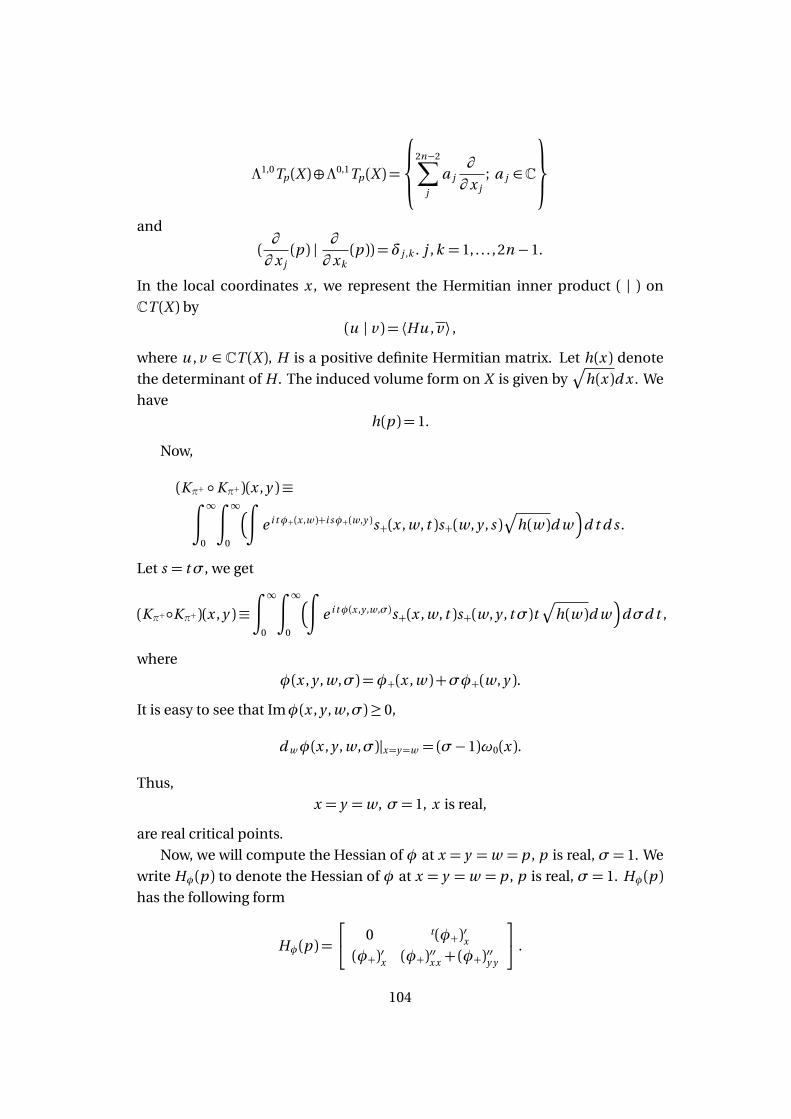
Λ1,0Tp (X )⊕Λ0,1Tp (X ) =
2n−2∑
j
a j∂
∂ x j; a j ∈C
and
(∂
∂ x j(p ) |
∂
∂ xk(p )) =δj ,k . j , k = 1, . . . , 2n −1.
In the local coordinates x , we represent the Hermitian inner product ( | ) on
CT (X ) by
(u | v ) = ⟨Hu , v ⟩ ,
where u , v ∈ CT (X ), H is a positive definite Hermitian matrix. Let h(x ) denote
the determinant of H . The induced volume form on X is given byp
h(x )d x . We
have
h(p ) = 1.
Now,
(Kπ+ Kπ+)(x , y )≡∫ ∞
0
∫ ∞
0
∫
e i tφ+(x ,w )+i sφ+(w ,y )s+(x , w , t )s+(w , y , s )p
h(w )d w
d t d s .
Let s = tσ, we get
(Kπ+Kπ+)(x , y )≡∫ ∞
0
∫ ∞
0
∫
e i tφ(x ,y ,w ,σ)s+(x , w , t )s+(w , y , tσ)tp
h(w )d w
dσd t ,
where
φ(x , y , w ,σ) =φ+(x , w )+σφ+(w , y ).
It is easy to see that Imφ(x , y , w ,σ)≥ 0,
d wφ(x , y , w ,σ)|x=y=w = (σ−1)ω0(x ).
Thus,
x = y =w , σ= 1, x is real,
are real critical points.
Now, we will compute the Hessian of φ at x = y =w = p , p is real, σ= 1. We
write Hφ(p ) to denote the Hessian of φ at x = y =w = p , p is real, σ = 1. Hφ(p )has the following form
Hφ(p ) =
0 t(φ+)′x(φ+)′x (φ+)′′x x +(φ+)
′′y y
.
104
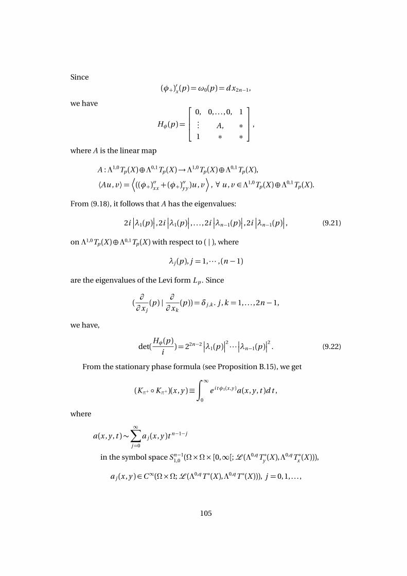
Since
(φ+)′x (p ) =ω0(p ) = d x2n−1,
we have
Hφ(p ) =
0, 0, . . . , 0, 1... A, ∗1 ∗ ∗
,
where A is the linear map
A :Λ1,0Tp (X )⊕Λ0,1Tp (X )→Λ1,0Tp (X )⊕Λ0,1Tp (X ),
⟨Au , v ⟩=D
((φ+)′′x x +(φ+)′′y y )u , v
E
, ∀ u , v ∈Λ1,0Tp (X )⊕Λ0,1Tp (X ).
From (9.18), it follows that A has the eigenvalues:
2i
λ1(p )
, 2i
λ1(p )
, . . . , 2i
λn−1(p )
, 2i
λn−1(p )
, (9.21)
on Λ1,0Tp (X )⊕Λ0,1Tp (X )with respect to ( | ), where
λj (p ), j = 1, · · · , (n −1)
are the eigenvalues of the Levi form L p . Since
(∂
∂ x j(p ) |
∂
∂ xk(p )) =δj ,k . j , k = 1, . . . , 2n −1,
we have,
det(Hφ(p )
i) = 22n−2
λ1(p )
2 · · ·
λn−1(p )
2. (9.22)
From the stationary phase formula (see Proposition B.15), we get
(Kπ+ Kπ+)(x , y )≡∫ ∞
0
e i tφ1(x ,y )a (x , y , t )d t ,
where
a (x , y , t )∼∞∑
j=0
a j (x , y )t n−1−j
in the symbol space Sn−11,0 (Ω×Ω× [0,∞[;L (Λ0,q T ∗y (X ),Λ
0,q T ∗x (X ))),
a j (x , y )∈C∞(Ω×Ω;L (Λ0,q T ∗(X ),Λ0,q T ∗(X ))), j = 0, 1, . . . ,
105
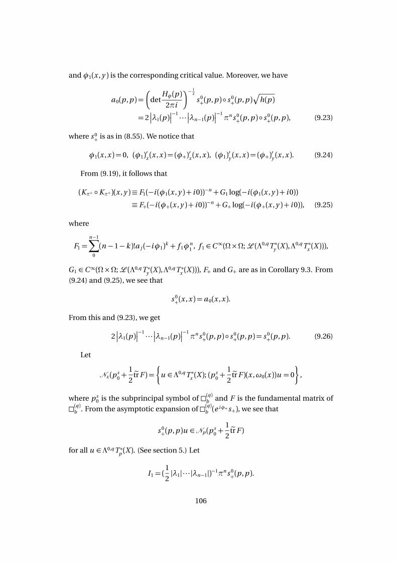
andφ1(x , y ) is the corresponding critical value. Moreover, we have
a 0(p , p ) =
detHφ(p )
2πi
− 12
s 0+(p , p ) s 0
+(p , p )p
h(p )
= 2
λ1(p )
−1 · · ·
λn−1(p )
−1πn s 0
+(p , p ) s 0+(p , p ), (9.23)
where s 0+ is as in (8.55). We notice that
φ1(x ,x ) = 0, (φ1)′x (x ,x ) = (φ+)′x (x ,x ), (φ1)′y (x ,x ) = (φ+)′y (x ,x ). (9.24)
From (9.19), it follows that
(Kπ+ Kπ+)(x , y )≡ F1(−i (φ1(x , y )+ i 0))−n +G1 log(−i (φ1(x , y )+ i 0))
≡ F+(−i (φ+(x , y )+ i 0))−n +G+ log(−i (φ+(x , y )+ i 0)), (9.25)
where
F1 =n−1∑
0
(n −1−k )!a j (−iφ1)k + f 1φn1 , f 1 ∈C∞(Ω×Ω;L (Λ0,q T ∗y (X ),Λ
0,q T ∗x (X ))),
G1 ∈C∞(Ω×Ω;L (Λ0,q T ∗y (X ),Λ0,q T ∗x (X ))), F+ and G+ are as in Corollary 9.3. From
(9.24) and (9.25), we see that
s 0+(x ,x ) = a 0(x ,x ).
From this and (9.23), we get
2
λ1(p )
−1 · · ·
λn−1(p )
−1πn s 0
+(p , p ) s 0+(p , p ) = s 0
+(p , p ). (9.26)
Let
Nx (p s0 +
1
2etr F ) =
u ∈Λ0,q T ∗x (X ); (ps0 +
1
2etr F )(x ,ω0(x ))u = 0
,
where p s0 is the subprincipal symbol of (q )b and F is the fundamental matrix of
(q )b . From the asymptotic expansion of (q )b (eiφ+s+), we see that
s 0+(p , p )u ∈Np (p s
0 +1
2etr F )
for all u ∈Λ0,q T ∗p (X ). (See section 5.) Let
I1 = (1
2|λ1| · · · |λn−1|)−1πn s 0
+(p , p ).
106
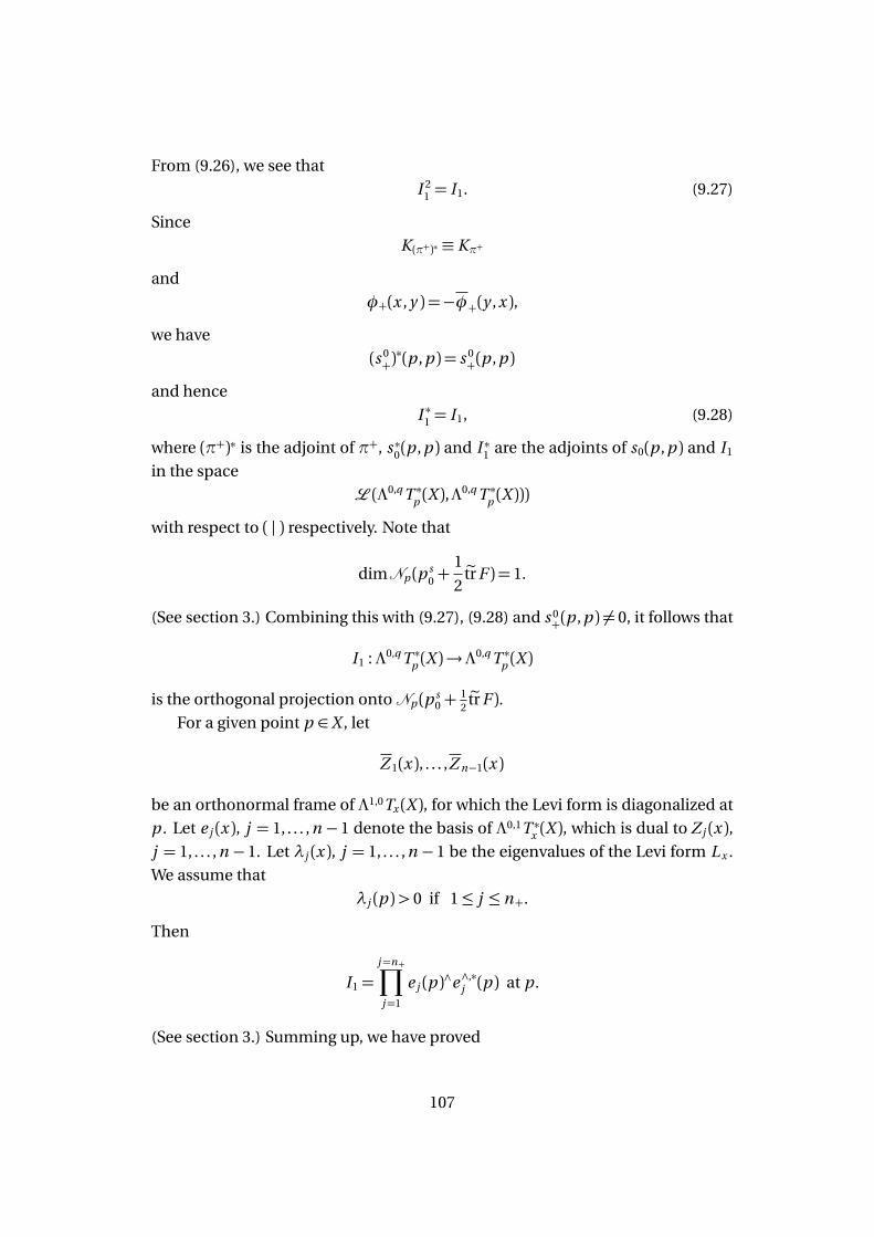
From (9.26), we see that
I 21 = I1. (9.27)
Since
K (π+)∗ ≡ Kπ+
and
φ+(x , y ) =−φ+(y ,x ),
we have
(s 0+)∗(p , p ) = s 0
+(p , p )
and hence
I ∗1 = I1, (9.28)
where (π+)∗ is the adjoint of π+, s ∗0(p , p ) and I ∗1 are the adjoints of s0(p , p ) and I1
in the space
L (Λ0,q T ∗p (X ),Λ0,q T ∗p (X )))
with respect to ( | ) respectively. Note that
dimNp (p s0 +
1
2etr F ) = 1.
(See section 3.) Combining this with (9.27), (9.28) and s 0+(p , p ) 6= 0, it follows that
I1 :Λ0,q T ∗p (X )→Λ0,q T ∗p (X )
is the orthogonal projection ontoNp (p s0 +
12etr F ).
For a given point p ∈X , let
Z 1(x ), . . . ,Z n−1(x )
be an orthonormal frame of Λ1,0Tx (X ), for which the Levi form is diagonalized at
p . Let e j (x ), j = 1, . . . , n − 1 denote the basis of Λ0,1T ∗x (X ), which is dual to Z j (x ),j = 1, . . . , n − 1. Let λj (x ), j = 1, . . . , n − 1 be the eigenvalues of the Levi form Lx .
We assume that
λj (p )> 0 if 1≤ j ≤ n+.
Then
I1 =j=n+∏
j=1
e j (p )∧e ∧,∗j (p ) at p .
(See section 3.) Summing up, we have proved
107
Proposition 9.4. For a given point x0 ∈X , Let
Z 1(x ), . . . ,Z n−1(x )
be an orthonormal frame of Λ1,0Tx (X ), for which the Levi form is diagonalized at
x0. Let e j (x ), j = 1, . . . , n − 1 denote the basis of Λ0,1T ∗x (X ), which is dual to Z j (x ),j = 1, . . . , n−1. Let λj (x ), j = 1, . . . , n−1 be the eigenvalues of the Levi form Lx . We
assume that q = n+ and that
λj (x0)> 0 if 1≤ j ≤ n+.
Then
F+(x0,x0) = (n −1)!1
2|λ1(x0)| · · · |λn−1(x0)|π−n
j=n+∏
j=1
e j (x0)∧e j (x0)∧,∗.
10 The Szegö projection on non-orientable CR man-ifolds
In this section, (X ,Λ1,0T (X )) is a compact connected not necessarily orientable
CR manifold of dimension 2n−1, n ≥ 2. We will use the same notations as before.
The definition of the Levi form (see 2.6) depends on the choices ofω0. However,
the number of non-zero eigenvalues is independent of the choices of ω0. Thus,
it makes sense to say that the Levi-form is non-degenerate. As before, we assume
that the Levi form L is non-degenerate at each point of X . We have the following
Lemma 10.1. Let (n−, n+), n− +n+ = n − 1, be the signature of the Levi-form L.
(The signature of the Levi-form L depends on the choices of ω0.) If n− 6= n+ at a
point of X , then X is orientable.
Proof. Since X is connected, n− 6= n+ at a point of X implies n− 6= n+ at each
point of X . Let X =⋃
Uj , where Uj is a local coordinate patch of X . On Uj , we
can choose an orthonormal frame
ω1,j (x ), . . . ,ωn−1,j (x )
for Λ1,0T ∗x (Uj ), then
ω1,j (x ), . . . ,ωn−1,j (x )
is an orthonormal frame for Λ0,1T ∗x (Uj ). The (2n −2)-form
ωj = i n−1ω1,j ∧ω1,j ∧ · · · ∧ωn−1,j ∧ωn−1,j
108
is real and is independent of the choice of the orthonormal frame. There is a real
1-form ω0,j (x ) of length one which is orthogonal to Λ1,0T ∗x (Uj )⊕Λ0,1T ∗x (Uj ). We
take ω0,j so that n− < n+ on Uj . Since ω0,j is unique up to sign and n− < n+ on
Uj , for all j , we have
ω0,j (x ) =ω0,k (x ) on Uj
⋂
Uk ,
soω0 is globally defined. The lemma follows.
We only need to consider the case n− = n+. We recall that if n− = n+ then(q )b
has closed range. In view of the proof of Theorem 8.20, we have the following
Theorem 10.2. Let (n−, n+) be the signature of the Levi form. We assume that
q = n− = n+. Put
Σ =
(x ,ξ)∈ T ∗(X ) \0; ξ=λω0(x ),λ 6= 0
,
whereω0 is the locally unique real 1 form determined up to sign by
‖ω0‖= 1, ω0⊥(Λ0,1T ∗(X )⊕Λ1,0T ∗(X )).
Then π is a well defined operator
π : H sloc (X ; Λ0,q T ∗(X ))→H s
loc (X ; Λ0,q T ∗(X )),
for all s ∈R, and
WF′(Kπ) = diag (Σ× Σ),
where
WF′(Kπ) =
(x ,ξ, y ,η)∈ T ∗(X )×T ∗(X ); (x ,ξ, y ,−η)∈WF(Kπ)
.
Here WF(Kπ) is the wave front set of Kπ in the sense of Hörmander [14].For every local coordinate patch U, we fix aω0 on U. We define
Σ+ =
(x ,ξ)∈ T ∗(U ) \0; ξ=λω0(x ),λ> 0
,
Σ− =
(x ,ξ)∈ T ∗(U ) \0; ξ=λω0(x ),λ< 0
.
We have
Kπ = Kπ+ +Kπ− on U ×U ,
where Kπ+(x , y ) satisfies
Kπ+(x , y )≡∫ ∞
0
e iφ+(x ,y )t s+(x , y , t )d t on U ×U
109
with
s+(x , y , t )∈Sn−11,0 (U ×U×]0,∞[;L (Λ0,q T ∗y (X ),Λ
0,q T ∗x (X ))),
s+(x , y , t )∼∞∑
j=0
s j+(x , y )t n−1−j
in the symbol space Sn−11,0 (U ×U×]0,∞[;L (Λ0,q T ∗y (X ),Λ
0,q T ∗x (X ))),
where
s j+(x , y )∈C∞(U ×U ;L (Λ0,q T ∗y (X ),Λ
0,q T ∗x (X ))), j = 0, 1, . . . ,
φ+(x , y )∈C∞(U ×U ),
φ+(x ,x ) = 0,
φ+(x , y ) 6= 0 if x 6= y ,
Imφ+(x , y )≥ 0,
d xφ+ 6= 0, d yφ+ 6= 0 where Imφ+ = 0,
d xφ+(x , y )|x=y =ω0(x ),
d yφ+(x , y )|x=y =−ω0(x ),
φ+(x , y ) =−φ+(y ,x ).
Moreover,φ+(x , y ) satisfies (9.18). Similarly,
Kπ−(x , y )≡∫ ∞
0
e iφ−(x ,y )t s−(x , y , t )d t modC∞
with
s−(x , y , t )∈Sn−11,0 (U ×U×]0,∞[;L (Λ0,q T ∗y (X ),Λ
0,q T ∗x (X ))),
s−(x , y , t )∼∞∑
j=0
s j−(x , y )t n−1−j
in the symbol space Sn−11,0 (U ×U×]0,∞[;L (Λ0,q T ∗y (X ),Λ
0,q T ∗x (X ))),
where
s j−(x , y )∈C∞(U ×U ;L (Λ0,q T ∗y (X ),Λ
0,q T ∗x (X ))), j = 0, 1, . . . ,
φ−(x , y ) =−φ+(x , y ).
110
A Appendix: Microlocal analysis, a review
We will give a brief discussion of microlocal analysis in a setting appropriate
for our purpose. For more details on the subject, see Hörmander [15], Grigis-
Sjöstrand [12] and Melin-Sjöstrand [18]. Our presentation is essentially taken
from Grigis-Sjöstrand [12] and Hörmander [15].Let Ω ⊂ Rn be an open set. From now on, we write xα = xα1
1 · · ·xαnn , ∂ αx =
∂ α1x1· · ·∂ αn
xn, Dα
x = Dα1x1· · ·Dαn
xnand |α| = α1 + · · ·+αn , where x = (x1, . . . ,xn ), Dx j =
−i∂x j . We have the following
Definition A.1. Let Ω⊂Rn be an open set. Let m ∈R. Sm (Ω×RN ) is the space of
all a ∈ C∞(Ω×RN ) such that for all compact sets K ⊂ Ω and all α ∈ Nn , β ∈ NN ,
there is a constant c > 0 such that
∂ αx ∂βξ a (x ,ξ)
≤ c (1+ |ξ|)m−|β |, (x ,ξ)∈ K ×RN .
Sm is called the space of symbols of order m . We write S−∞ =⋂
Sm , S∞ =⋃
Sm .
We next study asymptotic sums of symbols.
Proposition A.2. Let Ω ⊂ Rn be an open set. Let a j ∈ Sm j (Ω×RN ), j = 0, 1, 2, . . .
with m j −∞, j →∞. Then there exists a ∈Sm0(Ω×RN ) unique modulo (i.e. up
to some element in) S−∞(Ω×RN ), such that a −∑
0≤j<k a j ∈Smk (Ω×RN ), for every
k ∈N.
Proof. See Grigis-Sjöstrand [12] or Hörmander [14].
If a and a j have the properties of Proposition A.2, we write
a ∼∞∑
0
a j
and we call a the asymptotic sum of a j .
Definition A.3. LetΩ⊂Rn be an open set. The set Smcl (Ω×RN )of all a ∈Sm (Ω×RN )
such that
a (x ,ξ)∼∞∑
0
a j (x ,ξ),
where a j ∈C∞(Ω×RN ) is positively homogeneous of degree m − j when |ξ| ≥ 1,
will be called the space of classical symbols of order m .
The positively homogeneity in the definition means that
a j (x ,λξ) =λm−j a j (x ,ξ), |ξ| ≥ 1, λ≥ 1.
111
Definition A.4. Let Ω ⊂ Rn be an open set. A function ϕ(x ,ξ) ∈ C∞(Ω× RN ) is
called a phase function if for all (x ,ξ)∈Ω× RN :
(a) Imϕ(x ,ξ)≥ 0,
(b) ϕ(x ,λξ) =λϕ(x ,ξ) for all λ> 0,
(c) dϕ 6= 0.
Let Ω ⊂ Rn be an open set. Let D ′(Ω) be the space of Schwartz distributions
on Ω. Let
E ′(Ω) =
u ∈D ′(Ω); supp u is compact
.
Let ϕ(x ,ξ) be a phase function on Ω× RN and let a (x ,ξ) ∈Sm (Ω×RN ). Choose a
cut-off function χ(ξ) ∈ C∞(RN ) so that χ(ξ) = 1 when |ξ|< 1 and χ(ξ) = 0 when
|ξ|> 2. For all u ∈C∞0 (Ω), set
I (a ,ϕ)u = limε→0
∫
e iϕ(x ,ξ)a (x ,ξ)u (x )χ(εξ)d x dξ. (A.1)
Then I (a ,ϕ)∈D ′(Ω). More precisely, we have the following
Proposition A.5. Let Ω ⊂ Rn be an open set. Let ϕ(x ,ξ) be a phase function on
Ω×RN . Then there is a unique way of defining I (a ,ϕ)∈D ′(Ω) for a ∈S∞ such that
I (a ,ϕ) is defined by
I (a ,ϕ) =
∫
e iϕ(x ,ξ)a (x ,ξ)dξ
when a ∈Sm (Ω×RN ), m <−N and such that for every m ∈R, the map
Sm (Ω×RN )3 a → I (a ,ϕ)
is continuous.
Proof. See Grigis-Sjöstrand [12] or Hörmander [14].
Let Y ⊂ Rm1 , Z ⊂ Rm2 be open sets. We recall that the Schwartz kernel theo-
rem(see Hörmander [17]) states that there is a bijection between the set of distri-
butions K ∈D ′(Y ×Z ) and the set of continuous linear operators
A : C∞0 (Z )→D′(Y ).
The correspondence is given by
⟨Au , v ⟩Y = ⟨K , v ⊗u ⟩Y×Z , u ∈C∞0 (Z ), v ∈C∞0 (Y ),
112
where ⟨ , ⟩Y and ⟨ , ⟩Y×Z denote the duality brackes for D ′(Y )×C∞0 (Y ) and D ′(Y ×Z )×C∞0 (Y ×Z ) respectively and (v ⊗u )(y , z ) = v (y )u (z ). We call K the distribu-
tion kernel of A, and write K = KA . Moreover, the following two conditions are
equivalent:
(i) KA ∈C∞(Y ×Z ),
(ii) A is continuous E ′(Z )→C∞(Y ).
If A satisfies (i) or (ii), we say that A is smoothing. Let B be a continuous linear
operator
B : C∞0 (Z )→D′(Y ).
We write A ≡ B if A − B is a smoothing operator.
In order to simplify the discussion of composition of some operators, it is
convenient to introduce the notion of properly supported operators. Let C be a
closed subset of Y ×Z . We say that C is proper if the two projections
Πy : (y , z )∈C → y ∈ Y
Πz : (y , z )∈C → z ∈Z
are proper, that is the inverse image of every compact subset of Y and Z respec-
tively is compact.
A continuous linear operator
A : C∞0 (Z )→D′(Y )
is said to be properly supported if supp KA ⊂ Y ×Z is proper. If A is properly
supported, then A is continuous
C∞0 (Z )→E′(Y )
and A has a unique continuous extension
C∞(Z )→D ′(Y ).
Definition A.6. Let Y ⊂Rm1 , Z ⊂Rm2 be open sets. Let ϕ be a phase function on
Y ×Z × RN . Let a ∈Sm (Y ×Z ×RN ). Then a Fourier integral operator of order m
is a continuous linear map
A : C∞0 (Z )→D′(Y )
such that KA = I (a ,ϕ). Formally we write
Au (y ) =
∫ ∫
e iϕ(y ,z ,ξ)a (y , z ,ξ)u (z )d z dξ, u ∈C∞0 (Z ).
113
Definition A.7. Let Ω ⊂ RN be an open set. Let m ∈ R. A pseudodifferential
operator of order m is a continuous linear map:
A : C∞0 (Ω)→D′(Ω)
such that
KA =1
(2π)NI (a ,ϕ)
with a ∈Sm (Ω×Ω×RN ), ϕ(x , y ,ξ) = (x − y )ξ. Formally,
Au (x ) =1
(2π)N
∫ ∫
e i (x−y )ξa (x , y ,ξ)u (y )d y dξ, u ∈C∞0 (Ω).
We shall write Lm (Ω) to denote the space of pseudodifferential operators of order
m .
We collect some facts about pseudodifferential operators. For the proofs, see
Grigis-Sjöstrand [12] or Hörmander [15].Let Ω⊂RN be an open set. Let
Au (x ) =1
(2π)N
∫ ∫
e i (x−y )ξa (x , y ,ξ)u (y )d y dξ (A.2)
be a pseudodifferential operator of order m , where a ∈Sm (Ω×Ω×RN ). Then we
have the following properties:
(a) A is continuous
C∞0 (Ω)→C∞(Ω)
and has unique continuous extension
E ′(Ω)→D ′(Ω).
(b) If a ∈ S−∞(Ω×Ω×RN ), then KA ∈ C∞(Ω×Ω) and A is continuous E ′(Ω)→C∞(Ω), conversely if KA ∈ C∞, then there is a ∈ S−∞(Ω×Ω×RN ) such that
(A.2) holds.
We write L−∞(Ω) to denote the space of operators with a ∈S−∞(Ω×Ω×RN ).
(c) We recall that the singular support of KA is the smallest closed subset L of
Ω×Ω such that KA ∈ C∞((Ω×Ω) \ L). We write sing supp KA to denote the
singular support of KA . Then
sing supp KA ⊂ diag (Ω×Ω)= (x ,x )∈Ω×Ω .
114
(d) A has decomposition A = A ′+A ′′, where A ′ ∈ Lm (Ω) is properly supported
and A ′′ ∈ L−∞(Ω).
(e) Let A = A ′+A ′′ be the decomposition in (d). Set
A ′u (x ) =1
(2π)N
∫ ∫
e i (x−y )ξa (x , y ,ξ)u (y )d y dξ, u ∈C∞0 (Ω).
Then
a (x ,ξ) := e−i xξA ′(e i xξ)∈Sm (Ω×RN )
and has the asymptotic expansion
a (x ,ξ)∼∑
α∈NN
1
α!(∂ αξ Dα
y a (x , y ,ξ))
x=y. (A.3)
We call a (x ,ξ) the symbol of A. a (x ,ξ) is up to some element in S−∞(Ω×RN ). We write a (x ,ξ) =σA(x ,ξ). Moreover,
Au (x )≡1
(2π)N
∫
e i xξa (x ,ξ)u (ξ)dξ
=1
(2π)N
∫
e i⟨x−y ,ξ⟩a (x ,ξ)u (y )d y dξ,
where u (ξ) is the Fourier transform of u ∈C∞0 (Ω).
(f ) Let
(u | v ) =∫
u (y )v (y )d y
be the inner product on L2(Ω). We define the adjoint
A∗ : C∞0 (Ω)→D′(Ω)
by (Au | v ) = (u | A∗v ), u , v ∈C∞0 (Ω). The distribution kernel of A∗ is
KA∗(x , y ) = KA(y ,x )
and A∗ ∈ Lm (Ω). Moreover, σA∗ ∈ Sm and σA∗ has the following asymptotic
formula
σA∗(x ,ξ)∼∑
α∈NN
1
α!∂ αξ Dα
xσA(x ,ξ). (A.4)
(g) Let A ∈ Lm (Ω), B ∈ Lm ′(Ω), with at least one of A, B properly supported.
Then A B ∈ Lm+m ′(Ω) and
σAB (x ,ξ)∼∑
α∈NN
∂ αξ σA(x ,ξ)DαxσB (x ,ξ)
α!. (A.5)
115
(h) We writeS (RN ) to denote the set of allφ ∈C∞(RN ) such that
supx
xβ∂ αφ(x )
<∞
for all multi-indices α and β . Let S ′(RN ) be the dual space of S (RN ), i.e.
S ′(RN ) is the space of all continuous linear forms onS (RN ). We recall that
the Sobolev space H s (RN ), s ∈ R, is the space of all u ∈ S ′(RN ) such that
u (ξ) is locally square integrable and
‖u ‖2s =
1
(2π)N
∫
u (ξ)2
(1+ |ξ|2)s dξ<∞,
where u (ξ) is the Fourier transform of u . Define the Fréchet space
H sloc(Ω) =
¦
u ∈D ′(Ω); ϕa ∈H s (RN ), ∀ϕ ∈C∞0 (Ω)©
and
H scomp(Ω) =H s
loc(Ω)⋂
E ′(Ω).
If A ∈ Lm (Ω), then A is continuous
H scomp(Ω)→H s−m
loc (Ω).
If A ∈ Lm (Ω) is properly supported, then A is continuous
H sloc(Ω)→H s−m
loc (Ω).
Our next aim is to define pseudodifferential operators on a manifold. First
we must discuss changes of variables and the notions of principal symbol and
subprincipal sympol. Let κ : Ω→ Ωκ be a diffeomorphism map, where Ω, Ωκ are
open sets in RN . If A ∈ Lm (Ω), we want to study
eA = (κ−1)∗ A κ∗ : C∞0 (Ωκ)→C∞(Ωκ),
u ∈C∞0 (Ωκ)→ A(u κ) κ−1 ∈C∞(Ωκ).
We have the following
Proposition A.8. Let Ω, Ωκ ⊂RN be open sets. Let
κ :Ω→Ωκ
be a diffeomorphism. If A ∈ Lm (Ω). Then
eA = (κ−1)∗ A κ∗ ∈ Lm (Ωκ).
116
Moreover, we have the asymptotic expansion
σeA(κ(x ),ξ)∼
∑
α∈NN
∂ αξ a (x , tκ′(x )ξ)Dαy e i⟨ρx (y ),ξ⟩
α!
y=x
, (A.6)
where ρx (y ) = κ(y )−κ(x )−κ′(x )(y − x ) vanishes of second order at x . The terms
in the series are in Sm−| α2 |(Ω×RN ).
Proof. See Hörmander [14].
Definition A.9. LetΩ⊂RN be an open set. Let A ∈ Lm (Ω). We define the principal
symbol of A as the image ofσA in
(Sm/Sm−1)(Ω×RN ).
We then have a surjective map
Lm →Sm/Sm−1(Ω×RN )
which gives rise to a bijection
Lm/Lm−1→Sm/Sm−1(Ω×RN ).
Let Ω ⊂ RN be an open set. Let Lmcl (Ω) ⊂ Lm (Ω) be the space of pseudodif-
ferential operators A with σA ∈ Smcl . For such an operator we can identify the
principal symbol in Smcl /S
m−1cl with the positively homogenous function a m (x ,ξ)
in the asymptotic expansion
σA ∼∞∑
0
a m−j (x ,ξ), (A.7)
where a m−j (x ,ξ) is positively homogenous function of degree m − j .
Returning to the changes of variables for eA ∈ Lm (Ωκ), we see from (A.6) that
σeA(κ(x ),ξ)−σA(x , tκ′(x )ξ)∈Sm−1(Ω×RN ). (A.8)
If a , ea denote the principal symbols of A, eA, we get the relation
ea (κ(x ),ξ) = a (x , tκ′(x )ξ). (A.9)
Definition A.10. Let Ω⊂RN be an open set. Let A ∈ Lmcl (Ω) with symbol σA(x ,ξ)
as in (A.7). The subprincipal symbol of A is defined by
a s (x ,ξ) = a m−1(x ,ξ)+i
2
N∑
j=1
∂ 2a m (x ,ξ)∂ x j ∂ ξj
. (A.10)
117
Definition A.11. Let Ω⊂RN be an open set. Let A ∈ Lmcl (Ω) with symbol σA(x ,ξ)
as in (A.7). We say that (x0,ξ0) is a doubly characteristic point of A if
(a) a m (x0,ξ0) = 0,
(b) ( ∂ a m
∂ ξj)(x0,ξ0) = 0, j = 1, . . . , N ,
(c) ( ∂ a m
∂ x j)(x0,ξ0) = 0, j = 1, . . . , N .
We need the following (see Sjöstrand [21])
Lemma A.12. Let Ω⊂RN be an open set. Suppose that P = AQ1Q2+ B, where A ∈Lm
cl (Ω), Q1, Q2 ∈ L0cl(Ω), B ∈ Lm−1
cl (Ω) are properly supported classical pseudodiffer-
ential operators with principal symbols a , q1, q2, b respectively. Let ρ ∈ T ∗(Ω)r 0
be a point where q1 =q2 = 0. If we write the symbol of P as
p (x ,ξ) = pm (x ,ξ)+pm−1(x ,ξ)mod Sm−2
where pm and pm−1 are positively homogeneous of degree m and m − 1, then the
subprincipal symbol of P at ρ is given by the formula
p s (ρ) =b (ρ)+a (ρ)(2i )−1 q1,q2
(ρ).
In particular, if E ∈ Lkcl(Ω) is an elliptic operator with principal symbol e (x ,ξ), that
is e (x ,ξ) 6= 0, for all (x ,ξ) ∈Ω, then the subprincipal symbols of E P and P E at
ρ are e (ρ)p s (ρ).
Let Ω, Ωκ be open sets in RN . Let
κ :Ω→Ωκ
be a diffeomorphism. Let A ∈ Lmcl (Ω)with symbolσA(x ,ξ) as in (A.7). Let
eA = (κ−1)∗ A κ∗ ∈ Lmcl (Ωκ)
with symbol
σeA ∼
∞∑
j=0
ea m−j ,
where ea m−j is positively homogeneous of degree m − j . Let ρ = (x0, tκ′(x0)ξ0) be
a doubly characteristic point of A. From Taylor’s formula, we have
a m (x ,ξ) =2N∑
j ,k=1
a j ,k (x ,ξ)qj (x ,ξ)qk (x ,ξ) near ρ,
118
where a j ,k , j , k = 1, . . . , 2N , are positively homogeneous C∞ functions of degree
m and qj , j = 1, . . . , 2N , are positively homogeneous C∞ functions of degree 0
with qj (ρ) = 0, j = 1, . . . , 2N . If Q j ∈ L0cl(Ω) and A j ,k ∈ Lm
cl (Ω) are properly sup-
ported classical pseudodifferential operators with principal symbols qj and a j ,k
respectively, then
A =∑
j ,k
A j ,kQ jQk + B
near ρ, where B ∈ Lm−1cl (Ω). We denote the principal symbol of B by b . We have
eA =∑
j ,k
eA j ,k eQ j eQk + eB
near eρ = (κ(x0),ξ0), where eA j ,k = (κ−1)∗ A j ,k κ∗ ∈ Lmcl (Ωκ), eQ j = (κ−1)∗ Q j κ∗ ∈
Lmcl (Ωκ), eB = (κ
−1)∗ B κ∗ ∈ Lmcl (Ωκ). We denote the principal symbols by ea j ,k , eqj
and eb . From Lemma A.12, we have
a s (ρ) =b (ρ)+ (2i )−1∑
j ,k
a j ,k (ρ)¦
qj ,qk
©
(ρ)
and
ea s (eρ) =eb (eρ)+ (2i )−1∑
j ,k
ea j ,k (eρ)¦
eqj , eqk
©
(ρ),
where a s and ea s are the subprincipal symbols of A and eA respectively. In view of
(A.9), we have a s (ρ) = ea s (eρ). Summing up, we have proved
Proposition A.13. Let Ω, Ωκ be open sets in RN . Let
κ :Ω→Ωκ
be a diffeomorphism. Let A ∈ Lmcl (Ω)with symbolσA(x ,ξ) as in (A.7). Then
eA = (κ−1)∗ A κ∗ ∈ Lmcl (Ωκ)
with symbol
σeA ∼
∞∑
j=0
ea m−j ,
where ea m−j is positively homogeneous of degree m − j . We have
ea m (κ(x ),ξ) = a m (x , tκ′(x )ξ).
Moreover, if (x0, tκ′(x0)ξ0) is a doubly characteristic point of A, then (κ(x0),ξ0) is
also a doubly characteristic point of eA and
ea s (κ(x0),ξ0) = a s (x0, tκ′(x0)ξ0),
where a s , ea s denote the subprincipal symbols of A and eA respectively.
119
Definition A.14. Let m ∈R. A pseudodifferential operator of order m on a para-
compact C∞ manifold Ω is a continuous linear map
A : C∞0 (Ω)→C∞(Ω)
such that for every local coordinate patch Ωκ ⊂Ωwith coordinates
Ωκ 3 x → κ(x ) = (x1, . . . ,xN )∈ eΩκ ⊂RN ,
we have
(κ−1)∗ A κ∗ ∈ Lm (eΩκ).
We shall write A ∈ Lm (Ω) and extend A to a map
E ′(Ω)→D ′(Ω).
Definition A.15. Let Ω be a paracompact C∞ manifold of dimension N . Let m ∈R. Sm (T ∗(Ω)) is the set of all a ∈C∞(T ∗(Ω)) such that pullback to T ∗(eΩκ) = eΩκ×RN
is in Sm (eΩκ×RN ) for every coordinate patch Ωκ with coordinates eΩκ.
Definition A.16. LetΩbe a paracompact C∞manifold of dimension N . Smcl (T
∗(Ω))is the set of all a ∈Sm (T ∗(Ω)) such that pullback to T ∗(eΩκ) = eΩκ×RN is in Sm
cl (eΩκ×RN ) for every coordinate patch Ωκ with coordinates eΩκ. We call Sm
cl (T∗(Ω)) the
space of classical symbols of order m .
Lemma A.17. Let Ω1 and Ω2 be open sets in RN and let
φ :Ω1→Ω2
and
Φ :Ω1→GL (N ,R)(the group of invertible N ×N matrices)
be C∞ maps. Then
a 1(x ,ξ) = a 2(φ(x ),Φ(x )ξ)
is in Sm (Ω1×RN ) for every a 2 ∈Sm (Ω2×RN ).
Proof. See Hörmander [14].
From Lemma A.17, we see that to check that a ∈ Sm (T ∗(Ω)) it is enough to
check the requirement of Definition A.15 for an atlas and the definition agrees
with our earlier one if Ω⊂RN .
120
Definition A.18. Let Ω be a paracompact C∞ manifold of dimension N . If A ∈Lm (Ω) then the restriction of A to Ωκ identified with eΩκ defines a symbol in
Sm/S−∞(eΩκ×RN ),
where Ωκ is a local coordinate patch with coordinates eΩκ. If
a κ ∈Sm (T ∗(Ωκ))
is the pullback of a representative then
a κ−a κ′ ∈Sm−1(T ∗(Ωκ⋂
Ωκ′))
by Proposition A.8 for every pair of coordinate patches. With a locally finite par-
tition of unity¦
ψj
©
subordinate to a covering by coordinate patches Ωκj we set
a =∑
ψj a κj ∈Sm (T ∗(Ω))
and obtain
a −a κ ∈Sm−1(T ∗(Ωκ))
for every κ. This determines a modulo Sm−1(T ∗(Ω)) so we define the principal
symbol of A as the image of a in
Sm/Sm−1(T ∗(Ω)).
Let Ω be a paracompact C∞ manifold. Let A ∈ Lmcl (Ω) with symbol σA(x ,ξ) as
in (A.7). We identify the principal symbol of A with a m .
Definition A.19. Let Ω be a paracompact C∞ manifold. Let A ∈ Lm (Ω). If a ∈Sm (T ∗(Ω)) is the principal symbol of A then A is said to be non-characteristic at
(x0,ξ0)∈ T ∗(Ω)r0 if
ab −1∈S−1(T ∗(Ω))
in a conic neighborhood of (x0,ξ0) for some b ∈ S−m (T ∗(Ω)). We say that (x ,ξ) ∈T ∗(Ω) \ 0 is a characteristic point of A if (x ,ξ) is not a non-characteristic point of
A. Let Σ be the set of characteristic points of A. We call Σ the characteristic set of
A. Σ is a closed conic subset of T ∗(Ω) \0.
Let Ω be a paracompact C∞ manifold. Let A ∈ Lmcl (Ω) with symbol σA(x ,ξ) as
in (A.7). The condition of the definition A.19 is equivalent to a m (x0,ξ0) 6= 0 and
Σ=
(x ,ξ)∈ T ∗(Ω); a m (x ,ξ) = 0
.
121
Definition A.20. Let Ω be a paracompact C∞ manifold. Let A ∈ Lmcl (Ω) and let
Σ be the characteristic set of A. We say that (x ,ξ) ∈ Σ is a doubly characteristic
point of A if for every local coordinate patchΩκ, (x ,ξ)∈Ωκ, with local coordinateseΩκ, (x ,ξ) is a doubly characteristic point of eA, where eA is the pull back of A to eΩκ.
If every (x ,ξ) ∈Σ is a doubly characteristic point, we call Σ doubly characteristic
set.
Definition A.21. Let Ω be a paracompact C∞ manifold and let A ∈ Lmcl (Ω). Let
ρ = (x0,ξ0) be a doubly characteristic point of A. Let Ωκ, ρ ∈ Ωκ, be a local coor-
dinate patch with local coordinates eΩκ and let eA be the pull back of A to eΩκ. The
subprincipal symbol of A at ρ is the value ea s (ρ), where ea s is the subprincipal
symbol of eA.
In view of Proposition A.13, we see that the definition above makes sense. We
must review some facts about pseudodifferential operators between sections of
vector bundles. This will be important in this work.
Definition A.22. Let E and F be complex C∞ vector bundles over a C∞ manifold
Ω. Let m ∈R. Then a pseudodifferential operator of order m from sections of E
to sections of F is a continuous linear map
A : C∞0 (Ω; E )→C∞(Ω; F )
such that for every open set Y ⊂Ωwhere E and F are trivialized by
φE : EY → Y ×Ce , φF : FY → Y ×C f ,
there is a f × e matrix of pseudodifferential operators A j ,k ∈ Lm (Ω) such that
(φF (Au )|Y )j =∑
k
A j ,k (φE u )k , u ∈C∞0 (Y ; E ).
We shall then write A ∈ Lm (Ω; E , F ).
For every coordinate patch Ωκ ⊂Ω, let
v 1κ, v 2
κ, . . . , v eκ
and
w 1κ, w 2
κ, . . . , w fκ
be local frames of E and F respectively. Then, for every α ∈ C∞(Ωκ; E ) and a ∈C∞(Ωκ; F ), we have
α=∑
j
αjκ(x )v
jκ(x ), a =
∑
j
a jκ(x )w
jκ(x ),
122
where αjκ(x ), a j
κ(x )∈C∞(Ωκ). If Ωκ′⋂
Ωκ 6=φ, we write
α=∑
j
αjκv jκ =
∑
j
αjκ′v
jκ′ ,
a =∑
j
a jκw j
κ =∑
j
a jκ′w
jκ′ .
We have
α1κ′(x )
...
αeκ′(x )
= eκ′,κ(x )
α1κ(x )...
αeκ(x )
,
a 1κ′(x )
...
a fκ′(x )
= f κ′,κ(x )
a 1κ(x )...
a fκ(x )
,
where eκ′,κ(x ), f κ′,κ(x ) are the transition matrices of E and F respectively.
LetL (E , F ) be the vector bundle over T ∗(Ω) \ 0 with fiber at (x ,ξ) consisting
of the linear maps from Ex to Fx . Every α∈C∞(T ∗(Ω);L (E , F )) is represented by
α(x ,ξ) =
a j ,kvκ,wκ(x ,ξ)
,
α(x ,ξ) : Ex → Fx ,∑
j
s j v jκ(x )→
∑
j
t j w jκ(x ), t j =
∑
k
a j ,kvκ,wκ(x ,ξ)sk , x ∈Ωκ. (A.11)
If Ωκ⋂
Ωκ′ 6=φ, we have
a j ,kvκ′ ,wκ′
(x ,ξ)
= f κ′,κ(x )
a j ,kvκ,wκ(x ,ξ)
eκ,κ′(x ). (A.12)
We have the following
Definition A.23. Let E and F be complex C∞ vector bundles over a C∞ manifold
Ω. Let m ∈R. Sm (T ∗(Ω);L (E , F )) is the set of all
α∈C∞(T ∗(Ω);L (E , F ))
such that if we write α= (a j ,kvκwκ(x ,ξ)) as in (A.11), then
a j ,kvκ,wκ(x ,ξ)∈Sm (T ∗(Ωκ)) for every j , k .
Definition A.24. Let E and F be complex C∞ vector bundles over a C∞ manifold
Ω and let a (x ,ξ) ∈Sm (T ∗(Ω);L (E , F )). We say that a (x ,ξ) is a classical symbol, if
we write a (x ,ξ) =
a j ,kvκ,wκ(x ,ξ)
as in (A.11), then a j ,kvκ,wκ is a classical symbol, for
every j , k . We shall write Smcl (T
∗(Ω);L (E , F )) to denote the space of all classical
symbols.
123
Let E and F be complex C∞ vector bundles over a C∞ manifold Ω and let
A ∈ Lm (Ω; E , F ). For every coordinate patch Ωκ, we write
A = (A j ,kvκ,wκ), A j ,k
vκ,wκ∈ Lm (Ω),
A : C∞0 (Ωκ; E )→C∞(Ωκ; F ),∑
j
s j (x )v jκ(x ) 7→
∑
j
t j (x )w jκ(x ), t j =
∑
k
A j ,kvκ,wκ
sk . (A.13)
We define the symbol of A as
σA(x ,ξ) =
σAj ,kvκ ,wκ(x ,ξ)
.
If Ωκ′⋂
Ωκ 6=φ, we have
A j ,kvκ′ ,wκ′
= f κ′,κ(x )
A j ,kvκ,wκ
eκ,κ′(x ). (A.14)
From (A.14), we have
σAj ,kvκ′ ,wκ′(x ,ξ)
− f κ′,κ(x )
σAj ,kvκ ,wκ(x ,ξ)
eκ,κ′(x )∈Sm−1(T ∗(Ωκ′⋂
Ωκ);L (E , F )).(A.15)
We define the principal symbol of A at (x ,ξ)∈ T ∗(Ωκ) as the image ofσA(x ,ξ) in
(Sm/Sm−1)(T ∗(Ωκ);L (E , F )).
From (A.15), we see that the principal symbol of A is well-defined as an element
in
(Sm/Sm−1)(T ∗(Ω);L (E , F )).
We write Lmcl (Ω; E , F ) to denote the space of pseudodifferential operators of
order m from sections of E to sections of F withσA ∈Smcl (T
∗(Ω);L (E , F )).
Definition A.25. Let E and F be complex C∞ vector bundles over a C∞ manifold
Ω and let A ∈ Lmcl (Ω; E , F ). For every coordinate Ωκ, we write A = (A j ,k
vκ,wκ), A j ,kvκ,wκ ∈
Lm (Ωκ), as in (A.13). We say that (x0,ξ0) ∈ T ∗(Ωκ) \ 0 is a doubly characteristic
point of A if (x0,ξ0) is a doubly characteristic point of A j ,kvκ,wκ for every j , k .
Definition A.26. Let E and F be complex C∞ vector bundles over a C∞ manifold
Ω and let A ∈ Lmcl (Ω; E , F ). Let (x0,ξ0) be a doubly characteristic point of A. For
every coordinate Ωκ, (x0,ξ0) ∈ T ∗(Ωκ) \ 0, we write A = (A j ,kvκ,wκ), A j ,k
vκ,wκ ∈ Lm (Ωκ),as in (A.13). Let a s ,j ,k
vκ,wκ(x0,ξ0) be the subprincipal of A j ,k at (x0,ξ0), for every j , k .
From (A.14) and Lemma A.12 , we have
a s ,j ,kvκ′ ,wκ′
(x0,ξ0)
= f κ′,κ(x0)
a s ,j ,kvκ,wκ(x0,ξ0)
eκ,κ′(x0) (A.16)
124
on T ∗(Ωκ⋂
Ωκ′), where eκ′,κ(x ), f κ′,κ(x ) are the transition matrices of E and F re-
spectively. We define the subprincipal symbol of A at (x0,ξ0) as
a s ,j ,kvκ,wκ(x0,ξ0)
∈L (Ex0 , Fx0).
From (A.16), we see that the subprincipal of A is invariantly defined at every dou-
bly characteristic point of A.
We must make some comments on symplectic geometry. This will also be
important in this work. Our presentation is essentially taken from Duistermaat
[10], Hörmander [15] and Sjöstrand [21].First, we review some facts about symplectic vector spaces.
Definition A.27. An antisymmetric nondegenerate bilinear form on a finite di-
mensional vector space E is called a symplectic form on E . A symplectic vector
space is a pair (E ,σ) consisting of a finite dimensional vector space E and a sym-
plectic formσ on E .
σ is nondegenerate means that
σ(v, v ′) = 0, ∀v ′ ∈ E ⇒ v = 0.
Definition A.28. If (E1,σ1), (E2,σ2) are symplectic vector spaces and
T : E1→ E2
is a linear bijection with T ∗σ2 =σ1, that is
σ1(v, w ) =σ2(T v, Tw ), v, w ∈ E1,
then T is called a symplectic isomorphism.
In the vector space T ∗(Rn ) = (x ,ξ); x ,ξ∈Rn the symplectic form
σ=∑
dξj ∧d x j
is the bilinear form
σ((x ,ξ), (x ′,ξ′)) =
x ′ ,ξ
−
x ,ξ′
.
If e j and εj are the unit vectors along the x j and ξj axes respectively, then we
have for j , k = 1, . . . , n
σ(e j , ek ) =σ(εj ,εk ) = 0,
σ(εj , ek ) =−σ(ek ,εj ) =δj k
125
where δj k = 1 when j = k and δj k = 0 when j 6= k .
Let (E ,σ) be a symplectic vector space. Note that the linear bijection map-
ping
A : E → T ∗(Rn )
sending the vectors (e1, . . . , en , f 1, . . . , f n ) into the standard basis of T ∗(Rn ) is a
symplectic isomorphism if and only if for all j , k = 1, . . . , n
σ(e j , ek ) = 0,
σ( f j , f k ) = 0,
σ( f j , ek ) =δj ,k .
(A.17)
(e1, . . . , en , f 1, . . . , f n ) is called symplectic coordinates of (E ,σ)
Lemma A.29. Every symplectic vector space (E ,σ) admits a linear symplectic iso-
morphism
T : E → T ∗(Rn ).
Proof. See Duistermaat [10] or Hörmander [15].
If L is a linear subspace of E then we define its orthocomplement Lσ in E
with respect toσ by
Lσ = e ∈ E ;σ(e , l ) = 0 for all l ∈ L .
We have the following rules
L ⊂M ⇒Mσ ⊂ Lσ,
(Lσ)σ = L,
(L⋂
M )σ = Lσ+Mσ, (L+M )σ = Lσ⋂
Mσ,
dim Lσ = dim E −dim L.
Definition A.30. A linear subspace L of E is called isotropic, Lagrangian resp.
involutive, if L ⊂ Lσ, L = Lσ and L ⊃ Lσ respectively.
Definition A.31. A symplectic form on a manifold Ω is a 2-formσ on Ω such that
dσ= 0
and σρ is a symplectic form on Tρ(Ω), for each ρ ∈Ω. A symplectic manifold is a
pair (Ω,σ) consisting of a manifold Ω and a symplectic formσ on Ω.
126
Definition A.32. A submanifold V of a symplectic manifold is called symplectic,
isotropic, Lagrangian, involutive respectively, if at every point of V the tangent
space of V has this property.
Suppose (M ,σ), (N ,τ) are symplectic manifolds. Let
Φ : M →N
be a C∞-map. Let DΦ be the differential map, that is,
DΦρ : Tρ(M )→ Tρ(N )
v →d
d t(Φ α(t ))
t=0,
where α(t ) is a C 1-curve with α(0) =ρ and α′(0) = v .
Definition A.33. If (M ,σ), (N ,τ) are symplectic manifolds and
Φ : M →N
is a diffeomorphism withΦ∗τ=σ, that is, DΦρ is a symplectic isomorphism from
(Tρ(M ),σρ) to (TΦ(ρ)(N ),τΦ(ρ)) for all ρ ∈M , then Φ is called a canonical transfor-
mation.
Definition A.34. Let (M ,σ) be a symplectic manifold. For any f ∈ C∞(M ) the
Hamilton field H f is the unique C∞ vector field on M such that H f ùσ=−d f . We
notice that H f ùσ is a 1-form defined by
(H f ùσ)ρ(eρ) =σρ(H f (ρ), eρ),
where eρ ∈ Tρ(M ).
Definition A.35. Let (M ,σ) be a symplectic manifold. If f , g ∈ C∞(M ) then the
Poisson brackets
f , g
∈C∞(M ) are defined by
f , g
=H f g =σ(H f , Hg ).
Remark A.36. In symplectic coordinates (x ,ξ), we have
H f =∑
j
(∂ f
∂ ξj
∂
∂ x j−∂ f
∂ x j
∂
∂ ξj).
Let Ω be a C∞ manifold. Let
π : T ∗(Ω)→Ω
be the natural projection map.
127
Definition A.37. The canonical 1-form on T ∗(Ω) is the 1-form α given by
α(x ,ξ) = ξ Dπ(x ,ξ) for all (x ,ξ)∈ T ∗(Ω).
Definition A.38. σ= dσ is called the canonical 2-form on T ∗(Ω).
Remark A.39. (a) In canonical coordinates (x ,ξ)we have
α=∑
ξj d x j
and hence
σ=∑
dξj ∧d x j .
(b) T ∗(Ω)with canonical 2-formσ is a symplectic manifold.
Let (M ,σ) be a symplectic manifold. If
Φ : M → T ∗(Rn )
is a canonical transformation, then Φ is called a canonical coordinatization. It
is well-known that the functions x1, . . . ,xn ,ξ1, . . . ,ξn form local canonical coordi-
nates of (M ,σ) if and only if for all j , k = 1, . . . , n :
¦
x j ,xk
©
= 0,¦
ξj ,ξk
©
= 0,¦
ξj ,xk
©
=δj k .
We call x1, . . . ,xn ,ξ1, . . . ,ξn the symplectic coordinates of (M ,σ).
Proposition A.40. Suppose (M ,σ) is a symplectic manifold. Then dim M is even,
say 2n, and for each m0 ∈M there is a canonical coordinates of a neighborhood U
of m0.
Proof. See Duistermaat [10] or Hörmander [15].
Let (S,σ) be a symplectic vector space. Let Q(x ,ξ) be a real positive semi-
definite quadratic form in S. Let
Q(X , Y ) =
X ,Q ′′Y
be the corresponding symmetric form. Here Q ′′ is the Hessian of Q(x ,ξ). We have
the following definition
Definition A.41. The linear map F in S is defined by
σ(Y , F X ) =Q(Y , X ), X , Y ∈S
will be called the fundamental matrix of Q .
128
The symmetry of Q means that
σ(F X , Y ) =−σ(X , F Y ),
that is, F is skew symmetric with respect to σ. We notice that the preceding
definition is still applicable if Q is complex valued provied we replace S by its
complexification
SC = X + i Y ; X , Y ∈S
with the obvious complex symplectic structure.
Proposition A.42. Let Q(x ,ξ) be a real positive semi-definite quadratic form in S.
Let
Q(X , Y ) =
X ,Q ′′Y
be the corresponding symmetric form. Here Q ′′ is the Hessian of Q(x ,ξ). Then one
can choose symplectic coordinates x ,ξ such that
Q(x ,ξ) =k∑
j=1
1
2µj (x 2
j +ξ2j )+
k+l∑
k+1
x 2j
where µj > 0.
Proof. See Hörmander [15].
From Proposition A.42, we see that ±iµj are the non-vanishing eigenvalues
of the fundamental matrix F of Q . We write etr F =∑k
j=1
µj
.
Let Ω be a C∞ manifold of dimension n . Let p ∈ Ω and let f ∈ C 2(Ω) with
d f (p ) = 0. In local coordinates (x1, . . . ,xn ), we define
f ′′p =
∂ 2 f
∂ x j ∂ xk(p )
n
j ,k=1
.
Since d f (p ) = 0, f ′′p is well-defined as a linear map
f ′′p : Tp (Ω)→C,
t , s →D
t , f ′′p sE
,
where t , s ∈ Tp (Ω).If (S,σ) is a symplectic manifold and f ∈C 2(S) is real valued, d f = 0 at ρ ∈S.
Let Fρ be the fundamental matrix of f ′′ρ . We also call Fρ the fundamental matrix
of f . In symplectic coordinates (x ,ξ) the matrix F becomes
∂ 2 f∂ x∂ ξ
∂ 2 f∂ ξ∂ ξ
− ∂ 2 f∂ x∂ x
− ∂ 2 f∂ ξ∂ x
!
.
From this we see that the fundamental matrix F is the linearization of H f .
129
Remark A.43. The symplectic reduction of quadratic forms is an old topic in me-
chanics. It is also important for the study of hypoelliptic operators. See Boutet
de Monvel [7] and Sjöstrand [21].
B Appendix: Almost analytic manifolds, functions andvector fields
We will give a brief discussion of almost analytic manifolds, functions and vector
fields in a setting appropriate for our purpose. For more details on the subject,
see Melin-Sjöstrand [18].Let W ⊂Cn be an open set and let f ∈C∞(W ). In this section, we will use the
following notations:
∂ f =n∑
j=1
∂ f
∂ z jd z j
and
∂ f =n∑
j=1
∂ f
∂ z jd z j .
Definition B.1. Let W ⊂Cn be an open set and letφ(z ) be a positive continuous
function on W . If f ∈C∞(W ), we say that f is almost analytic with respect to the
weight function φ if, given any compact subset K of W and any integer N ≥ 0,
there is a constant c > 0 such that
∂ f (z )
≤ cφ(z )N , ∀z ∈ K .
Whenφ(z ) = |Im z |we simply say that f is almost analytic.
Definition B.2. Let f 1, f 2 ∈C∞(W )with W ,φ as above. We say that f 1 and f 2 are
equivalent with respect to the weight function φ if, given any compact subset K
of W and any integer N > 0, there is a constant c > 0 such that
( f 1− f 2)(z )
≤ cφ(z )N , ∀z ∈ K .
Whenφ(z ) = |Im z |we simply say that they are equivalent and we write
f 1 ∼ f 2.
The following proposition is due to Hörmander. For a proof, see [18].
Proposition B.3. Let W ⊂Cn be an open set and let WR =W⋂
Rn . If f ∈C∞(WR)then f has an almost analytic extension, uniquely determined up to equivalence.
130
Definition B.4. Let U be an open subset of Cn and let Λ be a C∞ submanifold of
codimension 2k of U . We say that Λ is an almost analytic manifold if for every
point z 0 of Λ⋂
Rn there exist an open neighborhood V of z 0 in U and k complex
C∞ almost analytic functions f 1, . . . , f k defined on V such that
Λ⋂
V is defined by the equations f 1(z ) = · · ·= f k (z ) = 0,
∂ f 1, . . . ,∂ f k are linearly independent over C at every point of V .
Definition B.5. Let Λ1 and Λ2 be two C∞ closed submanifolds of an open set
U ⊂Cn . We say that Λ1 and Λ2 are equivalent (and we write Λ1 ∼ Λ2) if they have
the same intersection with Rn and the same dimension and if for every open set
V ⊂⊂U and N ∈Nwe have
dist (z ,Λ2)≤ cN ,V |Im z |N , z ∈V⋂
Λ1, cN ,V > 0.
It is trivial that ∼ is an equivalence relation and that Λ1 and Λ2 are tangen-
tial to infinite order in the real points when Λ1 ∼ Λ2. We recall the Malgrange
preparation theorem (see Theorem 7.57 in Hörmander [17])
Theorem B.6. Let f j (t ,x ), j = 1, . . . , n, be complex valued C∞ functions in a neigh-
borhood of (0, 0) in Rn+m with f j (0, 0) = 0, j = 1, . . . , n, and
det
∂ f j (0, 0)∂ tk
n
j ,k=1
6= 0.
If g ∈C∞ in a neighborhood of (0, 0)we can then find qj (t ,x )∈C∞ in a neighbor-
hood of (0, 0), j = 1, . . . , n, and r (x )∈C∞ in a neighborhood of 0 so that
g (t ,x ) =n∑
j=1
qj (t ,x ) f j (t ,x )+ r (x )
in a neighborhood of (0, 0).
In section 8, we need the following
Proposition B.7. Let W be an open neighborhood of the origin in Cn+m . Let
f j (z , w ), g j (z , w ), j = 1, . . . , n, be almost analytic functions on W with f j (0, 0) = 0,
g j (0, 0) = 0, j = 1, . . . , n,
det
∂ f j (0, 0)∂ z k
n
j ,k=1
6= 0
and ∂ g 1, . . . ,∂ g n are linearly independent over C at the origin. Let
Λ1 =
(z , w )∈W ; f 1(z , w ) = . . .= f n (z , w ) = 0
131
and
Λ2 =
(z , w )∈W ; g 1(z , w ) = . . .= g n (z , w ) = 0
.
If Λ1 coincides to infinite order with Λ2 at (0, 0)we can then find a j ,k (z , w )∈C∞ in
a neighborhood of (0, 0), j , k = 1, . . . , n, with det
a j ,k (0, 0)n
j ,k=16= 0 so that
g j (z , w )−n∑
k=1
a j ,k (z , w ) f k (z , w )
vanishes to infinite order at (0, 0), for all j .
Proof. We write z = x + i y , w = u + i v , where x , y ∈ Rn , u , v ∈ Rm . From
Theorem B.6, it follows that
g j (x , u ) =n∑
k=1
a j ,k (x , u ) f k (x , u )+ r (u ), j = 1, . . . , n ,
in a real neighborhood of (0, 0), where a j ,k (x , u ) ∈ C∞ in a real neighborhood of
(0, 0), j , k = 1, . . . , n . Since Λ1 coincides to infinite order with Λ2 at (0, 0), it follows
that r (u ) vanishes to infinite order at 0. Since f k (0, 0) = 0, k = 1, . . . , n , we have
d g j (0, 0) =n∑
k=1
a j ,k (0, 0)d f k (0, 0), j = 1, . . . , n .
Hence
det
a j ,k (0, 0)n
j ,k=16= 0.
Let a j ,k (z , w ) be an almost analytic extension of a j ,k (x , u ) to a complex neigh-
borhood of (0, 0), where j , k = 1, . . . , n . Then
g j (z , w )−n∑
k=1
a j ,k (z , w ) f k (z , w )
also vanishes to infinite order at (0, 0), for all j .
We need the following
Lemma B.8. Let Ω, Ωκ be open sets in Rn . Let
κ :Ω→Ωκ
be a diffeomorphism. Let ΩC and ΩCκ be open sets in Cn with
ΩC⋂
Rn =Ω, ΩCκ⋂
Rn =Ωκ.
132
Let
eκ :ΩC→ΩCκbe an almost analytic extension of κ. We take ΩC and ΩCκ so that eκ is a diffeomor-
phism. If Λ is an almost analytic manifold of ΩC, then eκ(Λ) is an almost analytic
manifold of ΩCκ . Moreover, if
κ :ΩC→ΩCκis another almost analytic extension of κ and κ is a diffeomorphism, then
κ(Λ)∼ eκ(Λ).
Furthermore, if Λ1 ∼Λ2, then
eκ(Λ1)∼ eκ(Λ2),
where Λ1 and Λ2 are almost analytic manifolds of ΩC.
We shall now generalize the notion of almost analytic manifolds. We have the
following
Definition B.9. Let X be a n dimensional real paracompact C∞ manifold. An
almost analytic manifold Λ associated to X is given by
(a) A locally closed set ΛR. (Locally closed means that every point of ΛR has an
neighborhoodω in X such that ΛR⋂
ω is closed inω.)
(b) A covering of ΛR by open coordinate patches
κα : X ⊃Xα→Ωα ⊂Rn , α∈ J
and almost analytic manifolds Λα ⊂ΩCα with
Λα⋂
Rn :=ΛαR = κα(Xα⋂
ΛR).
Here ΩCα ⊂ Cn is some open set with ΩCα⋂
Rn = Ωα and the Λα shall satisfy
the following compatibility conditions: If
κβα = κβ κ−1α : κα(Xα
⋂
Xβ )→ κβ (Xα⋂
Xβ )
and if eκβα is an almost analytic extension of κβα, then eκβα(Λα) and Λβ are
equivalent near all points of κβ (Xα⋂
Xα⋂
ΛR).
The Λα are called local representatives of Λ and we shall say that two almost
analytic manifolds Λ, Λ′ associated to X are equivalent (and we write Λ ∼ Λ′) if
ΛR =Λ′R and if the corresponding local representatives are equivalent as in (b ).
133
Similarly we extend the notion of almost analytic functions and equivalence
of almost analytic functions.
Definition B.10. Let W be an open subset of Cn and let V be a complex C∞
vector field on W . We say that V is almost analytic if V ( f ) is almost analytic and
V ( f )∼ 0 for all almost analytic functions f on W .
We identify Cn with R2n . We shall denote the real coordinates by x j , y j , j =1, . . . , n , and the complex coordinates by z j = x j + i y j , j = 1, . . . , n .
Definition B.11. Let W be an open subset of Cn and let
U =n∑
j=1
a j (z )∂
∂ z j+
n∑
j=1
b j (z )∂
∂ z j,
V =n∑
j=1
c j (z )∂
∂ z j+
n∑
j=1
d j (z )∂
∂ z j,
be complex C∞ vector fields on W , where
a j (z ),b j (z ), c j (z ), d j (z )∈C∞(W ), j = 1, . . . , n .
We say that U and V are equivalent if
a j (z )− c j (z )∼ 0, b j (z )−d j (z )∼ 0
for all j . If U and V are equivalent, we write
U ∼V.
Clearly U is almost analytic if and only if
U ∼n∑
j=1
a j (z )∂
∂ z j,
where a j , j = 1, . . . , n , are almost analytic. We have the following easy lemma
Lemma B.12. Let W be an open subset of Cn and let V be an almost analytic
vector field on W . Then
V ( f )∼ (V +V )( f ) for all almost analytic functions f . (B.1)
If U is a real vector field on W and
U ( f )∼V ( f ) for all almost analytic functions f ,
then
U ∼V +V .
134
We have the following
Proposition B.13. Let W be an open subset of Cn and let Σ be a C∞ closed sub-
manifold of Rn . Let V be an almost analytic vector field on W . We assume that
V = 0 on Σ.
Let Φ(t ,ρ) be the V +V flow. Let U be a real vector field on W such that
U ∼V +V .
Let Φ(t ,ρ) be the U flow. Then, for every compact set K ⊂ W , N ≥ 0, there is a
cN ,K (t )> 0, such that
Φ(t ,ρ)− Φ(t ,ρ)
≤ cN ,K (t )dist (ρ,Σ)N , ρ ∈ K .
Proof. We have the following well-known fact: If Z is a smooth vector field on an
open set Ω ⊂ Rn with Z (x0) = 0 and Ψ(t ,x ) = exp (t Z )(x ), then Ψ(t ,x0) = x0 and
∂ αx Ψ(t ,x )|x=x0 , α ∈ Nn , only depend on (∂ βx Z )(x0), β ∈ Nn . In our situation, we
therefore have that Φ(t ,ρ), Φ(t ,ρ) have the same Taylor expansion at every point
of Σ.
The following proposition is useful (see section 2 of Melin-Sjöstrand [18])
Proposition B.14. Assume that f (x , w ) is a C∞ complex function in a neighbor-
hood of (0, 0) in Rn+m and that
Im f ≥ 0, Im f (0, 0) = 0, f ′x (0, 0) = 0, det f ′′x x (0, 0) 6= 0. (B.2)
Let ef (z , w ), z = x + i y , w ∈ Cm , denote an almost analytic extension of f to a
complex neighborhood of (0, 0) and let z (w ) denote the solution of
∂ ef
∂ z(z (w ), w ) = 0
in a neighborhood of 0 in Cm . Then,
∂
∂w( ef (z (w ), w ))−
∂
∂wef (z , w )|z=z (w ), w is real
vanishes to infinite order at 0∈Rm . (B.3)
Moreover, there is a constant c > 0 such that near the origin we have
Im ef (z (w ), w )≥ c |Im z (w )|2 , w ∈Rm (B.4)
and
Im ef (z (w ), w )≥ c infx∈Ω
Im f (x , w )+
d x f (x , w )
2
, w ∈Rm , (B.5)
where Ω is some open set of the origin in Rn .
We call ef (z (w ), w ) the corresponding critical value.
135
Proof. For a proof of (B.4), see [18]. We only prove (B.5). In view of the proof of
(B.4) (see p.147 of [18]), we see that
Im ef (z (w ), w )≥ c
inft∈Rn ,|t |≤1
Im f (Re z (w )− t |Im z (w )| , w )+ |Im z (w )|2
(B.6)
for w small, where w is real and c is a positive constant. Using the almost ana-
lyticity, we get by Taylor’s formula:
f ′x (x , w ) = f ′′z z (z (w ), w )(x − z (w ))+O(|x − z (w )|2+ |Im z (w )|2) (B.7)
for x , w small, where w is real. Since f ′′z z is invertible near the origin, we have
that when w ∈Rm is close to the origin,
|Im z (w )|2 ≥ c
f ′x (Re z (w )− t |Im z (w )| , w )
2
for all t ∈ Rn , |t | ≤ 1, where c is a positive constant. From this and (B.6), we get
(B.5).
In the following, we let z = z (w ) be the point defined as above. We recall the
stationary phase formula of Melin and Sjöstrand
Proposition B.15. Let f (x , w ) be as in Proposition B.14. Then there are neighbor-
hoods U and V of the origin in Rn and Rm respectively and differential operators
C f ,j in x of order ≤ 2j which are C∞ functions of w ∈V such that
∫
e i t f (x ,w )u (x , w )d x−
det
t ef ′′z z (z (w ), w )2πi
!
− 12e i t ef (z (w ),w )
N−1∑
0
(C f ,j eu )(z (w ), w )t −j
≤ cN t −N− n2 , t ≥ 1, (B.8)
where u ∈ C∞0 (U × V ). Here ef and eu are almost analytic extensions of f and u
respectively. The function
det
t ef ′′z z (z (w ), w )2πi
!
− 12
is the branch of the square root of
det
t ef ′′z z (z (w ), w )2πi
!
−1
which is continuously deformed into 1 under the homotopy
s ∈ [0, 1]→ i−1(1− s ) ef ′′z z (z (w ), w )+ s I ∈GL (n ,C).
136
We need the following asymptotic formula (see Melin-Sjöstrand [18])
Proposition B.16. Let P ∈ Lm (Rn ) and let ϕ(x ) ∈ C∞(Rn ) satisfy Imϕ ≥ 0 and
dϕ 6= 0 where Imϕ = 0. Let u (x )∈C∞0 (Rn ). If p (x ,ξ) is the full symbol of P, then
P(e i tϕ(x )u (x ))∼ e i tϕ(x )∑
α
1
α!ep (α)(x , tϕ′x (x ))
1
α!Dα
y (u (y )ei tρ(x ,y ))|y=x (B.9)
with asymptotic convergence in Sm0,1(Rn×R+), where ep is an almost analytic exten-
sion of p and
ρ(x , y ) =ϕ(y )−ϕ(x )−¬
y −x ,ϕ′x (x )¶
.
Definition B.17. The C∞ function ϕ(x ,θ ) defined in an open conic set V ⊂Rn ×RN \0 is called a non-degenerate complex phase function if
(a) dϕ 6= 0.
(b) ϕ(x ,θ ) is positively homogeneous of degree 1.
(c) Put
C =¦
(x ,θ )∈V ; ϕ′θ (x ,θ ) = 0©
.
The differentials d ( ∂ ϕ∂ θj), j = 1, . . . , N , are linearly independent over the com-
plex numbers on C .
(d) Imϕ ≥ 0.
Letφ(x ,θ ) be a non-degenerate complex phase function in a conic open sub-
set Γ of Rn × RN . Let
Cφ =¦
(x ,θ )∈ Γ;φ′θ (x ,θ ) = 0©
.
By Euler’s homogeneity relation, we have φ(x ,θ ) = θ .φ′θ (x ,θ ) = 0 on Cφ and
therefore Imφ vanishes on Cφ. So does d (Imφ), for otherwise there would be a
change of sign of Imφ.
Let eφ be an almost analytic extension of φ in a conic open set eΓ ⊂ Cn × CN ,eΓ⋂
(Rn × RN ) = Γ. We can choose eφ such that eφ is homogeneous of degree 1. Set
eφ′eθ= (∂
eθ1eφ, . . . ,∂
eθNeφ)
andeφ′ex = (∂ex1
eφ, . . . ,∂exneφ).
Let
Ceφ =¦
(ex , eθ )∈ eΓ; eφ′eθ(ex , eθ ) = 0
©
, (B.10)
Λeφ =¦
(ex , eφ′ex (ex , eθ )); (ex , eθ )∈C
eφ
©
. (B.11)
137
Λeφ is an almost analytic manifold and
(Λeφ)R =Λ eφ
⋂
(Rn × Rn ) =¦
(x ,φ′x (x ,θ )); (x ,θ )∈Cφ©
.
Let eφ1 be another almost analytic extension ofφ in eΓ. We have
Λeφ ∼Λ eφ1
.
(See [18].) Moreover, we have the following
Proposition B.18. For every point (x0,ξ0) ∈ (Λ eφ)R and after suitable change of
local x coordinates, Λeφ is equivalent to a manifold
−ex =∂ h(eξ)
∂ eξ, eξ∈CN
in some open neighborhood of (x0,ξ0), where h is an almost analytic function and
Im h ≥ 0 on RN with equality at ξ0.
Definition B.19. An almost analytic manifold satisfying the conditions of Propo-
sition B.18 at every real point for some real symplectic coordinate (x ,ξ) is called
a positive Lagrangean manifold.
Letϕ andψbe non-degenerate phase functions defined in small conic neigh-
borhoods of (x0,θ0)∈Rn×RN and (x0, w0)∈Rn×RM respectively. We assume that
ϕ′θ (x0,θ0) = 0,ψ′w (x0, w0) = 0 and that
ϕ′x (x0,θ0) =ψ′x (x0, w0) = ξ0,
where the last equation is a definition. Put λ0 = (x0,ξ0). We have the following
definition
Definition B.20. We say that ϕ and ψ are equivalent at λ0 for classical symbols
if there is a conic neighborhood Λ of (x0,θ0) such that for every distribution
A =
∫
e iϕ(x ,θ )a (x ,θ )dθ ,
where a (x ,θ )∈Smcl (Rn ×RN )with support in Λ, there exists
b (x , w )∈Sm+N−M
2cl (Rn ×RM )
with support in a conic neighborhood of (x0,ω0) such that
A − B ∈C∞,
where B =∫
e iψ(x ,w )b (x , w )d w and vise versa.
138
The global theory of Fourier integral operators with complex phase is the fol-
lowing
Proposition B.21. Let ϕ and ψ be non-degenerate phase functions defined in
small conic neighborhoods of (x0,θ0) ∈ Rn × RN and (x0, w0) ∈ Rn × RM respec-
tively. We assume that ϕ′θ (x0,θ0) = 0,ψ′w (x0, w0) = 0 and that
ϕ′x (x0,θ0) =ψ′x (x0, w0) = ξ0.
Then ϕ andψ are equivalent at (x0,ξ0) for classical symbols if and only if Λeϕ and
Λeψ are equivalent in some neighborhood of (x0,ξ0), where eϕ and eψ are almost
analytic extensions of ϕ andψ respectively and Λeϕ, Λ
eψ are as in (B.11).
References
[1] R. Beals and P. Greiner, Calculus on Heisenberg manifolds, Annals of Math-
ematics Studies, no. 119, Princeton University Press, Princeton, NJ, 1988.
[2] R. Berman, Bergman kernel asymptotics and holomorphic Morse inequali-
ties, Ph.D. thesis, Chalmers University of Technology and Göteborg Univer-
sity, Göteborg, Sweden, April 2006.
[3] R. Berman and J. Sjöstrand, Asymptotics for Bergman-Hodge kernels for high
powers of complex line bundles, arXiv.org/abs/math.CV/0511158.
[4] B. Berndtsson, R. Berman, and J. Sjöstrand, Asymptotics of Bergman kernels,
arXiv.org/abs/math.CV/050636.
[5] A. Boggess, CR manifolds and the tangential Cauchy-Riemann complex,
Studies in Advanced Mathematics, CRC Press, 1991.
[6] S.-C. Chen and M.-C Shaw, Partial differential equations in several complex
variables, AMS/IP Studies in Advanced Mathematics, vol. 19, Amer. Math.
Soc., 2001.
[7] L. Boutet de Monvel, Hypoelliptic operators with double characteristics and
related pseudo-differential operators, Comm. Pure Appl. Math. 27 (1974),
585–639.
[8] L. Boutet de Monvel and V. Guillemin, The spectral theory of toeplitz opera-
tors, Annals of Mathematics Studies, vol. 99, Princeton University Press, NJ;
University of Tokyo Press, Tokyo, 1981.
139
[9] L. Boutet de Monvel and J. Sjöstrand, Sur la singularité des noyaux de
Bergman et de Szegö, Astérisque 34-35 (1976), 123–164.
[10] J. J. Duistermaat, Fourier integral operators, Progress in Mathmatics, vol.
130, Birkhäuser Boston, Inc., Boston, MA, 1996.
[11] G. B. Folland and J. J. Kohn, The Neumann problem for the Cauchy-Riemann
complex, Annals of Mathematics Studies, no. 75, Princeton University Press,
Princeton, NJ, University of Tokyo Press, Tokyo, 1972.
[12] A. Grigis and J. Sjöstrand, Microlocal analysis for differential operators. An
introduction, London Mathematical Society Lecture Note Series, vol. 196,
Cambridge University Press, Cambridge, 1994.
[13] B. Helffer and J. Sjöstrand, Semiclassical analysis for Harper’s equation. III.
Cantor structure of the spectrum, Mém. Soc. Math. France (N.S.) (1989),
no. 39, 1–124.
[14] L. Hörmander, Fourier integral operators, I, Acta Math. 127 (1971), 79–183.
[15] , The analysis of linear partial differential operators III pseudodif-
ferential operators, Grundlehren der Mathematischen Wissenschaften, vol.
274, Springer-Verlag, Berlin, 1985.
[16] , The analysis of linear partial differential operators IV Fourier inte-
gral operators, Grundlehren der Mathematischen Wissenschaften, vol. 275,
Springer-Verlag, Berlin, 1985.
[17] , The analysis of linear partial differential operators I distribution the-
ory and Fourier analysis, Classics in Mathematics, Springer-Verlag, Berlin,
2003.
[18] A. Melin and J. Sjöstrand, Fourier integral operators with complex-valued
phase functions, Springer Lecture Notes in Math, vol. 459, pp. 120–223,
Springer-Verlag, Berlin, 1974.
[19] , Fourier integral operators with complex phase and parametrix for
an interior boundary value problem, Comm. Partial Diff. Eqns. 1(4) (1976),
313–400.
[20] A. Menikoff and J. Sjöstrand, On the eigenvalues of a class of hypoelliptic
operators, Math. Ann. 235 (1978), 55–85.
140
[21] J. Sjöstrand, Parametrices for pseudodifferential operators with multiple
characteristics, Ark. Mat. 12 (1974), 85–130.
[22] F. Treves, Introduction to pseudodifferential and Fourier integral operators II
Fourier integral operators, Plenum Press, New York, NY, 1980.
141

On the singularities of the Bergmanprojection for (0,q ) forms
Chin-Yu Hsiao
Abstract
We obtain the full asymptotic expansion of the Bergman projec-
tion for (0,q ) forms when the Levi form is non-degenerate. This gen-
eralizes a result of Boutet de Monvel and Sjöstrand for (0, 0) forms.
We introduce a new operator analogous to the Kohn Laplacian de-
fined on the boundary of a domain and we apply the heat equation
method of Menikoff and Sjöstrand to this operator. We obtain a de-
scription of a new Szegö projection up to smoothing operators. Fi-
nally, by using the Poisson operator, we get our main result.
Résumé
Nous obtenons un développement asymptotique de la singular-
ité du noyau de Bergman pour les (0,q ) formes quand la forme de
Levi est non-dégénérée. Cela généralise un résultat de Boutet de
Monvel et Sjöstrand pour les (0, 0) formes. Nous introduisons un
nouvel opérateur analogue au laplacien de Kohn, défini sur le bord
du domaine et nous y appliquons la méthode de Menikoff-Sjöstrand.
Cela donne une description modulo des opéreateurs régularisants
d’un nouvel projecteur de Szegö. Finalement, en utilisant l’opérateur
de Poisson, nous obtenons notre résultat principal.
Contents
1 Introduction and statement of the main results 2
2 Terminology and notations, a review 14
3 The ∂ -Neumann problem, a review 22
4 The operator T 26
1
5 The principal symbols of γ∂ P and γ∂ f∗P 31
6 The operator(q )β 35
7 The heat equation for(q )β 40
8 The Bergman projection 53
9 Examples 669.1 Complex projective space . . . . . . . . . . . . . . . . . . . . . . . . . . . . . . . 68
9.2 Spherical shell in Cn . . . . . . . . . . . . . . . . . . . . . . . . . . . . . . . . . . . 73
A Appendix: The wave front set of a distribution, a review 74
1 Introduction and statement of the main results
In this paper, we assume that all manifolds are paracompact. (For the precise
definition, see page 156 of Kelley [19].) Let M be a relatively compact open sub-
set with C∞ boundary Γ of a complex manifold M ′ of dimension n with a smooth
Hermitian metric ( | ) on its holomorphic tangent bundle. (See (1.1).) The Hermi-
tian metric induces a Hermitian metric on the bundle of (0,q ) forms of M ′ (see
the discussion after (1.1) and section 2) and a positive density (d M ′)(see (1.3)).
Let be the ∂ -Neumann Laplacian on M (see Folland and Kohn [9] or (1.6))
and let (q ) denote the restriction to (0,q ) forms. For p ∈ Γ, let L p be the Levi
form of Γ at p (see (1.12) or Definition 2.2). Given q , 0 ≤ q ≤ n − 1, the Levi
form is said to satisfy condition Z (q ) at p ∈ Γ if it has at least n − q positive or
at least q + 1 negative eigenvalues. When condition Z (q ) holds at each point of
Γ, Kohn’s L2 estimates give the hypoellipicity with loss of one dervative for the
solutions of (q )u = f . (See [9] or Theorem 3.6.) The Bergman projection is the
orthogonal projection onto the kernel of (q ) in the L2 space. When condition
Z (q ) fails at some point of Γ, one is interested in the Bergman projection on the
level of (0,q ) forms. When q = 0 and the Levi form is positive definite, the exis-
tence of the complete asymptotic expansion of the singularities of the Bergman
projection was obtained by Fefferman [8] on the diagonal and subsequently by
Boutet de Monvel and Sjöstrand (see [7]) in complete generality. If q = n −1 and
the Levi form is negative definite, Hörmander [17] obtained the corresponding
asymptotics for the Bergman projection in the distribution sense. We have been
influenced by these works.
We now start to formulate the main results. First, we introduce some nota-
tions. Let Ω be a C∞ manifold. We let T (Ω) and T ∗(Ω) denote the tangent bundle
2
of Ω and the cotangent bundle of Ω respectively. The complexified tangent bun-
dle of Ω and the complexified cotangent bundle of Ω will be denoted by CT (Ω)and CT ∗(Ω) respectively. Let E be a C∞ vector bundle over Ω. The fiber of E at
x ∈ Ω will be denoted by Ex . Let Y ⊂⊂ Ω be an open set. The spaces of smooth
sections of E over Y and distribution sections of E over Y will be denoted by
C∞(Y ; E ) and D ′(Y ; E ) respectively. Let E ′(Y ; E ) be the subspace of D ′(Y ; E )of sections with compact support in Y . For s ∈ R, we let H s (Y ; E ) denote the
Sobolev space of order s of sections of E over Y . Put
H sloc (Y ; E ) =¦
u ∈D ′(Y ; E ); ϕu ∈H s (Y ; E ), ∀ϕ ∈C∞0 (Y )©
and
H scomp (Y ; E ) =H s
loc(Y ; E )⋂
E ′(Y ; E ).
Let F be a C∞ vector bundle over M ′. Let C∞(M ; F ), D ′(M ; F ), H s (M ; F ) denote
the spaces of restrictions to M of elements in C∞(M ′; F ),D ′(M ′; F ) and H s (M ′; F )respectively. Let C∞0 (M ; F ) be the subspace of C∞(M ; F ) of sections with com-
pact support in M .
Let Λ1,0T (M ′) and Λ0,1T (M ′) be the holomorphic tangent bundle of M ′ and
the anti-holomorphic tangent boundle of M ′ respectively. (See (2.4).) In local
coordinates z = (z 1, . . . , z n ), we represent the Hermitian metric on Λ1,0T (M ′) by
(u | v ) = g (u , v ), u , v ∈Λ1,0T (M ′),
g =n∑
j ,k=1
g j ,k (z )d z j ⊗d z k , (1.1)
where g j ,k (z ) = g k ,j (z ) ∈C∞, j , k = 1, . . . , n , and
g j ,k (z )n
j ,k=1is positive definite
at each point. We extend the Hermitian metric ( | ) toCT (M ′) in a natural way by
requiring Λ1,0T (M ′) to be orthogonal to Λ0,1T (M ′) and satisfy
(u | v ) = (u | v ), u , v ∈Λ0,1T (M ′).
The Hermitian metric ( | ) on CT (M ) induces, by duality, a Hermitian metric
on CT ∗(M ) that we shall also denote by ( | ). (See (2.9).) For q ∈N, let Λ0,q T ∗(M ′)be the bundle of (0,q ) forms of M ′. (See (2.6).) The Hermitian metric ( | ) on
CT ∗(M ′) induces a Hermitian metric on Λ0,q T ∗(M ′) also denoted by ( | ). (See
(2.11).)
Let r ∈C∞(M ′) be a defining function of Γ such that r is real, r = 0 on Γ, r < 0
on M and d r 6= 0 near Γ. From now on, we take a defining function r so that
‖d r ‖= 1 on Γ.
3
The Hermitian metric ( | ) on CT (M ′) induces a Hermitian metric ( | ) on
CT (Γ). For z ∈ Γ, we identify CT ∗z (Γ)with the space
¦
u ∈CT ∗z (M′); (u | d r ) = 0©
. (1.2)
We associate to the Hermitian metric∑n
j ,k=1 g j ,k (z )d z j⊗d z k a real (1, 1) form
( see page 144 of Kodaira [20])
ω= in∑
j ,k=1
g j ,k d z j ∧d z k .
Let
d M ′ =ωn
n !(1.3)
be the volume element (see also (2.12)) and let ( | )M be the inner product on
C∞(M ; Λ0,q T ∗(M ′)) defined by
( f | h)M =∫
M
( f | h)(d M ′) =
∫
M
( f | h)ωn
n !, f , h ∈C∞(M ; Λ0,q T ∗(M ′)). (1.4)
Similarly, we take (dΓ) as the induced volume form on Γ (see (2.18)) and let ( | )Γbe the inner product on C∞(Γ; Λ0,q T ∗(M ′)) defined by
( f | g )Γ =∫
Γ
( f | g )dΓ, f , g ∈C∞(Γ; Λ0,q T ∗(M ′)). (1.5)
Let4Γ be the real Laplacian on Γ and denote byσ4Γ the principal symbol of4Γ.
Let
∂ : C∞(M ′; Λ0,q T ∗(M ′))→C∞(M ′; Λ0,q+1T ∗(M ′))
be the part of the exterior differential operator which maps forms of type (0,q ) to
forms of type (0,q +1) and we denote by
∂ f∗
: C∞(M ′; Λ0,q+1T ∗(M ′))→C∞(M ′; Λ0,q T ∗(M ′))
the formal adjoint of ∂ . That is
(∂ f | h)M ′ = ( f | ∂ f∗h)M ′ , f ∈C∞0 (M
′; Λ0,q T ∗(M ′)), h ∈C∞(M ′; Λ0,q+1T ∗(M ′)),
where ( | )M ′ is defined by
(g | k )M ′ =
∫
M ′
(g | k )(d M ′), g , k ∈C∞0 (M′; Λ0,q T ∗(M ′)).
4
We shall also use the notation ∂ for the closure in L2 of the ∂ operator, initially
defined on C∞(M ; Λ0,q T ∗(M ′)) and ∂∗
for the Hilbert space adjoint of ∂ . The do-
main of ∂∗
consists of all f ∈ L2(M ; Λ0,q+1T ∗(M ′)) such that for some constant
c > 0,
( f | ∂ g )M
≤ c
g
, for all g ∈C∞(M ; Λ0,q T ∗(M ′)).
For such an f ,
g → ( f | ∂ g )M
extends to a bounded anti-linear functional on L2(M ; Λ0,q T ∗(M ′)) so
( f | ∂ g )M = ( ef | g )M
for some ef ∈ L2(M ; Λ0,q T ∗(M ′)). We have ∂∗
f = ef . The ∂ -Neumann Laplacian on
(0,q ) forms is then the self-adjoint operator in the space L2(M ; Λ0,q T ∗(M ′)) (see
chapter I of [9])(q ) = ∂ ∂
∗+ ∂
∗∂ . (1.6)
We notice that
Dom(q ) = u ∈ L2(M ; Λ0,q T ∗(M ′)); u ∈Dom∂∗⋂
Dom∂ ,
∂∗u ∈Dom∂ , ∂ u ∈Dom∂
∗ (1.7)
and C∞(M ; Λ0,q T ∗(M ′))⋂
Dom(q ) is dense in Dom(q ). (See also page 14 of [9].)Let
(q )f = ∂ ∂ f∗+ ∂ f
∗∂ : C∞(M ′; Λ0,q T ∗(M ′))→C∞(M ′; Λ0,q T ∗(M ′)) (1.8)
denote the complex Laplace-Beltrami operator on (0,q ) forms and denote by
σ(q )fthe principal symbol of (q )f . Let γ denote the operator of restriction to the
boundary Γ. Let us consider the map:
F (q ) : H 2(M ; Λ0,q T ∗(M ′))→H 0(M ; Λ0,q T ∗(M ′))⊕H32 (Γ; Λ0,q T ∗(M ′)),
u → ((q )f u ,γu ). (1.9)
Given q , 0≤q ≤ n −1, we assume that
Assumption 1.1. F (k ) is injective, q −1≤ k ≤q +1.
Thus, the Poisson operator for (k )f , q − 1 ≤ k ≤ q + 1, is well-defined. (See
section 4.) If M ′ is Kähler, then F (q ) is injective for any q , 0≤ q ≤ n . (See section
9 for the definition and details.)
5
We write ⟨ , ⟩ to denote the duality between Tz (M ′) and T ∗z (M′). We extend ⟨ , ⟩
bilinearly to CTz (M ′)×CT ∗z (M′). Let ∂
∂ rbe the dual vector of d r . That is
(u |∂
∂ r) = ⟨u , d r ⟩ , (1.10)
for all u ∈CT (M ′). Put
ω0 = J t (d r ), (1.11)
where J t is the complex structure map for the cotangent bundle. (See (2.2).)
Let Λ1,0T (Γ) and Λ0,1T (Γ) be the holomorphic tangent bundle of Γ and the
anti-holomorphic tangent bundle of Γ respectively. (See (2.22).) The Levi form
L p (Z , W ), p ∈ Γ, Z , W ∈ Λ1,0Tp (Γ), is the Hermitian quadratic form on Λ1,0Tp (Γ)defined as follows:
For any Z , W ∈Λ1,0Tp (Γ), pick eZ , fW ∈C∞(Γ; Λ1,0T (Γ)) that satisfy
eZ (p ) =Z , fW (p ) =W . Then L p (Z , W ) =1
2i
D
[eZ ,fW ](p ) ,ω0(p )E
.(1.12)
The eigenvalues of the Levi form at p ∈ Γ are the eigenvalues of the Hermitian
form L p with respect to the inner product ( | ) on Λ1,0Tp (Γ). If the Levi form is
non-degenerate at p ∈ Γ, let (n−, n+), n−+n+ = n−1, be the signature and notice
that Z (q ) holds at p if and only if q 6= n−.
We recall the Hörmander symbol spaces
Definition 1.2. Let m ∈R. Let U be an open set in M ′×M ′.
Sm1,0(U×]0,∞[;L (Λ0,q T ∗y (M
′),Λ0,q T ∗x (M′)))
is the space of all a (x , y , t ) ∈ C∞(U×]0,∞[;L (Λ0,q T ∗y (M′),Λ0,q T ∗x (M
′))) such that
for all compact sets K ⊂ U and all α ∈ N2n , β ∈ N2n , γ ∈ N, there is a constant
c > 0 such that
∂ αx ∂β
y ∂γ
t a (x , y , t )
≤ c (1+ |t |)m−|γ|, (x , y , t )∈ K×]0,∞[.
Sm1,0 is called the space of symbols of order m type (1, 0). We write S−∞1,0 =
⋂
Sm1,0.
Let Sm1,0(U⋂
(M ×M )×]0,∞[;L (Λ0,q T ∗w (M′),Λ0,q T ∗z (M
′))) denote the space of
restrictions to U⋂
(M ×M )×]0,∞[ of elements in
Sm1,0(U×]0,∞[;L (Λ0,q T ∗w (M
′),Λ0,q T ∗z (M′))).
Let
a j ∈Sm j
1,0 (U⋂
(M ×M )×]0,∞[;L (Λ0,q T ∗w (M′),Λ0,q T ∗z (M
′))), j = 0, 1, 2, . . . ,
6
with m j −∞, j →∞. Then there exists
a ∈Sm01,0 (U⋂
(M ×M )×]0,∞[;L (Λ0,q T ∗w (M′),Λ0,q T ∗z (M
′)))
such that
a −∑
0≤j<k
a j ∈Smk1,0 (U⋂
(M ×M )×]0,∞[;L (Λ0,q T ∗w (M′),Λ0,q T ∗z (M
′))),
for every k ∈N. (See Proposition 1.8 of Grigis-Sjöstrand [11] or Hörmander [13].)If a and a j have the properties above, we write
a ∼∞∑
j=0
a j in the space Sm01,0 (U⋂
(M ×M )× [0,∞[;L (Λ0,q T ∗w (M′),Λ0,q T ∗z (M
′))).
Let
Π(q ) : L2(M ; Λ0,q T ∗(M ′))→Ker(q )
be the Bergman projection, i.e. the orthogonal projection onto the kernel of(q ).Let
KΠ(q )(z , w )∈D ′(M ×M ;L (Λ0,q T ∗w (M′),Λ0,q T ∗z (M
′)))
be the distribution kernel of Π(q ). Formally,
(Π(q )u )(z ) =
∫
M
KΠ(q )(z , w )u (w )d M ′(w ), u (w )∈C∞0 (M ; Λ0,q T ∗(M ′)).
Let X and Y be C∞ vector bundles over M ′. Let
C , D : C∞0 (M ; X )→D ′(M ; Y )
with distribution kernels
KC (z , w ), KD(z , w )∈D ′(M ×M ;L (Xw , Yz )).
We write
C ≡D mod C∞(U⋂
(M ×M ))
if
KC (z , w ) = KD(z , w )+ F (z , w ),
where F (z , w )∈C∞(U⋂
(M ×M );L (Xw , Yz )) and U is an open set in M ′×M ′.
Given q , 0≤q ≤ n −1. Put
Γq =
z ∈ Γ; Z (q ) fails at z
. (1.13)
If the Levi form is non-degenerate at each point of Γ, then Γq is a union of con-
nected components of Γ.
The main result of this work is the following
7
Theorem 1.3. Let M be a relatively compact open subset with C∞ boundary Γ of
a complex analytic manifold M ′ of dimension n. We assume that the Levi form is
non-degenerate at each point of Γ. Let q, 0≤ q ≤ n −1. Suppose that Z (q ) fails at
some point of Γ and that Z (q −1) and Z (q +1) hold at each point of Γ. Then
KΠ(q )(z , w )∈C∞(M ×M \diag (Γq ×Γq );L (Λ0,q T ∗w (M′),Λ0,q T ∗z (M
′))).
Moreover, in a neighborhood U of diag (Γq ×Γq ), KΠ(q )(z , w ) satisfies
KΠ(q )(z , w )≡∫ ∞
0
e iφ(z ,w )t b (z , w , t )d t mod C∞(U⋂
(M ×M )) (1.14)
(for the precise meaning of the oscillatory integral∫∞
0e iφ(z ,w )t b (z , w , t )d t , see Re-
mark 1.4 below) with
b (z , w , t )∈Sn1,0(U⋂
(M ×M )×]0,∞[;L (Λ0,q T ∗w (M′),Λ0,q T ∗z (M
′))),
b (z , w , t )∼∞∑
j=0
b j (z , w )t n−j
in the space Sn1,0(U⋂
(M ×M )×]0,∞[;L (Λ0,q T ∗w (M′),Λ0,q T ∗z (M
′))),
b0(z , z ) 6= 0, z ∈ Γq ,
where
b j (z , w )∈C∞(U⋂
(M ×M );L (Λ0,q T ∗w (M′),Λ0,q T ∗z (M
′))), j = 0, 1, . . . ,
and
φ(z , w )∈C∞(U⋂
(M ×M )), (1.15)
φ(z , z ) = 0, z ∈ Γq , (1.16)
φ(z , w ) 6= 0 if (z , w ) /∈ diag (Γq ×Γq ), (1.17)
Imφ ≥ 0, (1.18)
Imφ(z , w )> 0 if (z , w ) /∈ Γ×Γ, (1.19)
φ(z , w ) =−φ(w , z ). (1.20)
For p ∈ Γq , we have
σ(q )f(z , d zφ(z , w )) vanishes to infinite order at z = p ,
(z , w ) is in some neighborhood of (p , p ) in M ′. (1.21)
8
For z =w , z ∈ Γq , we have
d zφ =−ω0− i d r,
d wφ =ω0− i d r.
Moreover, we have
φ(z , w ) =φ−(z , w ) if z , w ∈ Γq ,
whereφ−(z , w )∈C∞(Γq×Γq ) is the phase appearing in the description of the Szegö
projection in [18]. See Theorem 1.5 and Theorem 7.15 below.
Remark 1.4. Letφ(z , w ) and b (z , w , t ) be as in Theorem 1.3. Let y = (y1, . . . , y2n−1)be local coordinates on Γ and extend y1, . . . , y2n−1 to real smooth functions in
some neighborhood of Γ. We work with local local coordinates
w = (y1, . . . , y2n−1, r )
defined on some small neighborhood U of p ∈ Γq . Let u ∈ C∞0 (U ; Λ0,q T ∗(M ′)).Choose a cut-off function χ(t )∈C∞(R) so that χ(t ) = 1 when |t |< 1 and χ(t ) = 0
when |t |> 2. Set
(Bεu )(z ) =
∫ ∫ ∞
0
e iφ(z ,w )t b (z , w , t )χ(εt )u (w )d t d w .
Since d yφ 6= 0 where Imφ = 0 (see (7.31)), we can integrate by parts in y and t
and obtain
limε→0(Bεu )(z )∈C∞(M ; Λ0,q T ∗(M ′)).
This means that
B = limε→0
Bε : C∞(M ; Λ0,q T ∗(M ′))→C∞(M ; Λ0,q T ∗(M ′))
is continuous. We write B (z , w ) to denote the distribution kernel of B . Formally,
B (z , w ) =
∫ ∞
0
e iφ(z ,w )t b (z , w , t )d t .
From (1.21) and Remark 1.5 of [18] it follows that
Theorem 1.5. Under the assumptions of Theorem 1.3, let p ∈ Γq . We choose local
complex analytic coordinates
z = (z 1, . . . , z n ), z j = x2j−1+ i x2j , j = 1, . . . , n ,
9
vanishing at p such that the metric on Λ1,0T (M ′) is
n∑
j=1
d z j ⊗d z j at p
and
r (z ) =p
2Im z n +n−1∑
j=1
λj
z j
2+O(|z |3),
where λj , j = 1, . . . , n − 1, are the eigenvalues of L p . (This is always possible. See
Lemma 3.2 of [17].) We also write
w = (w1, . . . , wn ), w j = y2j−1+ i y2j , j = 1, . . . , n .
Then, we can takeφ(z , w ) so that
φ(z , w ) =−p
2x2n−1+p
2y2n−1− i r (z )
1+2n−1∑
j=1
a j x j +1
2a 2n x2n
− i r (w )
1+2n−1∑
j=1
a j y j +1
2a 2n y2n
+ in−1∑
j=1
λj
z j −w j
2
+n−1∑
j=1
iλj (z j w j − z j w j )+O
|(z , w )|3
(1.22)
in some neighborhood of (p , p ) in M ′×M ′, where
a j =1
2
∂ σ(q )f
∂ x j(p ,−ω0(p )− i d r (p )), j = 1, . . . , 2n .
We have the following corollary of Theorem 1.3
Corollary 1.6. Under the assumptions of Theorem 1.3 and let U be a small neigh-
borhood of diag (Γq ×Γq ). Then there exist smooth functions
F,G ∈C∞(U⋂
(M ×M ));L (Λ0,q T ∗w (M′),Λ0,q T ∗z (M
′)))
such that
KΠ(q ) = F (−i (φ(z , w )+ i 0))−n−1+G log(−i (φ(z , w )+ i 0)).
Moreover, we have
F =n∑
j=0
(n − j )!b j (z , w )(−iφ(z , w ))j + f (z , w )(φ(z , w ))n+1,
G ≡∞∑
j=0
(−1)j+1
j !bn+j+1(z , w )(−iφ(z , w ))j mod C∞(U
⋂
(M ×M )) (1.23)
10
where
f (z , w )∈C∞(U⋂
(M ×M );L (Λ0,q T ∗w (M′),Λ0,q T ∗z (M
′))).
If w ∈Λ0,1T ∗z (M′), let
w ∧,∗ :Λ0,q+1T ∗z (M′)→Λ0,q T ∗z (M
′) (1.24)
be the adjoint of left exterior multiplication
w ∧ :Λ0,q T ∗z (M′)→Λ0,q+1T ∗z (M
′).
That is,
(w ∧u | v ) = (u |w ∧,∗v ), (1.25)
for all u ∈Λ0,q T ∗z (M′), v ∈Λ0,q+1T ∗z (M
′). Notice that w ∧,∗ depends anti-linearly on
w .
Let Λ0,1T ∗(Γ) be the bundle of boundary (0, 1) forms. (See (2.23) and (2.29).)
Proposition 1.7. Under the assumptions of Theorem 1.3, let p ∈ Γq , q = n−. Let
Z 1(z ), . . . ,Z n−1(z )
be an orthonormal frame of Λ1,0Tz (Γ), z ∈ Γ, for which the Levi form is diagonal-
ized at p . Let e j (z ), j = 1, . . . , n − 1 denote the basis of Λ0,1T ∗z (Γ), z ∈ Γ, which is
dual to Z j (z ), j = 1, . . . , n − 1. Let λj (z ), j = 1, . . . , n − 1 be the eigenvalues of the
Levi form L z , z ∈ Γ. We assume that
λj (p )< 0 if 1≤ j ≤ n−.
Then
F (p , p ) = n !
λ1(p )
· · ·
λn−1(p )
π−n 2
j=n−∏
j=1
e j (p )∧e ∧,∗j (p )
(∂ r (p ))∧,∗(∂ r (p ))∧,
(1.26)
where F is as in Corollary 1.6.
In the rest of this section, we outline the proof of Theorem 1.3. We assume
that the Levi form is non-degenerate at each point of Γ. We pause and recall a
general fact of distribution theory. (See Hörmander [16].) Let E , F be C∞ vector
bundles over C∞ manifolds G and H respectively. We take smooth densities of
integration on G and H respectively. Let
A : C∞0 (G ; E )→D ′(H ; F )
with distribution kernel
KA(x , y )∈D ′(H ×G ;L (Ey , Fx )).
Then the following two statements are equivalent
11
(a) A is continuous: E ′(G ; E )→C∞(H ; F ),
(b) KA ∈C∞(H ×G ;L (Ey , Fx )).
If A satisfies (a) or (b), we say that A is smoothing. Let
B : C∞0 (G ; E )→D ′(H ; F ).
From now on, we write K B (x , y ) or B (x , y ) to denote the distribution kernel of B
and we write
A ≡ B
if A − B is a smoothing operator.
Let
P : C∞(Γ; Λ0,q T ∗(M ′))→C∞(M ; Λ0,q T ∗(M ′)) (1.27)
be the Poisson operator for (q )f which is well-defined since we assumed (1.9) to
be injective. It is well-known that P extends continuously
P : H s (Γ; Λ0,q T ∗(M ′))→H s+ 12 (M ; Λ0,q T ∗(M ′)), ∀ s ∈R.
(See page 29 of Boutet de Monvel [5].) Let
P∗ : E ′(M ; Λ0,q T ∗(M ′))→D ′(Γ; Λ0,q T ∗(M ′))
be the operator defined by
(P∗u | v )Γ = (u | Pv )M , u ∈ E ′(M ; Λ0,q T ∗(M ′)), v ∈C∞(Γ; Λ0,q T ∗(M ′)).
It is well-known (see page 30 of [5]) that P∗ is continuous:
P∗ : L2(M ; Λ0,q T ∗(M ′))→H12 (Γ; Λ0,q T ∗(M ′))
and
P∗ : C∞(M ; Λ0,q T ∗(M ′))→C∞(Γ; Λ0,q T ∗(M ′)).
We use the inner product [ | ] on H− 12 (Γ; Λ0,q T ∗(M ′)) defined as follows:
[u | v ] = (Pu | Pv )M ,
where u , v ∈H− 12 (Γ; Λ0,q T ∗(M ′)). We consider (∂ r )∧,∗ as an operator
(∂ r )∧,∗ : H− 12 (Γ; Λ0,q T ∗(M ′))→H− 1
2 (Γ; Λ0,q−1T ∗(M ′)).
Note that (∂ r )∧,∗ is the pointwise adjoint of ∂ r with respect to ( | ). Let
T : H− 12 (Γ; Λ0,q T ∗(M ′))→Ker (∂ r )∧,∗ (1.28)
12
be the orthogonal projection onto Ker (∂ r )∧,∗ with respect to [ | ]. That is, if u ∈H− 1
2 (Γ; Λ0,q T ∗(M ′)), then
(∂ r )∧,∗Tu = 0
and
[(I −T )u | g ] = 0, ∀ g ∈Ker (∂ r )∧,∗.
In section 4, we will show that T is a classical pseudodifferential operator of order
0 with principal symbol
2(∂ r )∧,∗(∂ r )∧.
For q ∈ N, let Λ0,q T ∗(Γ) be the bundle of boundary (0,q ) forms. (See (2.29).) If
u ∈C∞(Γ; Λ0,q T ∗(M ′)), then u ∈Ker (∂ r )∧,∗ if and only if u ∈C∞(Γ; Λ0,q T ∗(Γ)). Put
∂β = Tγ∂ P : C∞(Γ; Λ0,q T ∗(Γ))→C∞(Γ; Λ0,q+1T ∗(Γ)). (1.29)
∂β is a classical pseudodifferential operator of order one from boundary (0,q )forms to boundary (0,q +1) forms. It is easy to see that
∂β = ∂b + lower order terms, (1.30)
where ∂b is the tangential Cauchy-Riemann operator. (See [9] or section 6.) In
section 6, we will show that
(∂β )2 = 0.
Let
∂β†
: C∞(Γ; Λ0,q+1T ∗(Γ))→C∞(Γ; Λ0,q T ∗(Γ)),
be the formal adjoint of ∂β with respect to [ | ]. ∂β†
is a classical pseudodifferential
operator of order one from boundary (0,q+1) forms to boundary (0,q ) forms. In
section 6, we will show that
∂β†= γ∂ f
∗P.
Put
(q )β = ∂β ∂β†+ ∂β
†∂β : C∞(Γ; Λ0,q T ∗(Γ))→C∞(Γ; Λ0,q T ∗(Γ)).
For simplicity, we assume that Γ = Γq , Γq 6= Γn−1−q . We can repeat the method
of [18] (see section 7) to construct
A ∈ L−112 , 1
2
(Γ; Λ0,q T ∗(Γ),Λ0,q T ∗(Γ)), B ∈ L012 , 1
2
(Γ; Λ0,q T ∗(Γ),Λ0,q T ∗(Γ))
such that
A(q )β + B ≡ B +(q )β A ≡ I ,
∂βB ≡ 0, ∂β†B ≡ 0,
B ≡ B † ≡ B 2,
13
where Lm12 , 1
2
is the space of pseudodifferential operators of order m type ( 12
, 12) (see
Definition 7.11) and B † is the formal adjoint of B with respect to [ | ]. Moreover,
K B (x , y ) satisfies
K B (x , y )≡∫ ∞
0
e iφ−(x ,y )t b (x , y , t )d t ,
where φ−(x , y ) and b (x , y , t ) are as in Theorem 7.15. In section 8, we will show
that
Π(q ) ≡ P BT (P∗P)−1P∗ mod C∞(M ×M )
and
P BT (P∗P)−1P∗(z , w )≡∫ ∞
0
e iφ(z ,w )t b (z , w , t )d t mod C∞(M ×M ),
whereφ(z , w ) and b (z , w , t ) are as in Theorem 1.3.
Acknowledgements. The author would like to thank his advisor Johannes Sjös-
trand for his patience, guidance and inspiration.
2 Terminology and notations, a review
In this section, we will review some standard terminology in complex geometry.
For more details on the subject, see Kodaira [20].Let E be a finite dimensional vector space with a complex structure J . By
definition, a complex structure J is a R-linear map
J : E → E
that satisfies
J 2 =−I .
Let CE be the complexification of E . That is,
CE = u + i v ; u , v ∈ E .
Any vector in CE can be written
f = u + i v
where u , v ∈ E and anyR-linear map between real vector spaces can be extended
to a C-linear map between the complexifications, simply by putting
T f = Tu + i T v.
14

In particular, we can extend J to a C-linear map
J :CE →CE .
Clearly, it still holds that J 2 = −I . This implies that we have a decomposition as
a direct sum
CE =Λ1,0E ⊕Λ0,1E
where
J u = i u if u ∈Λ1,0E
and
J u =−i u if u ∈Λ0,1E .
Let us now return to our original situation where E = Tp (M ′), p ∈M ′. Given
holomorphic coordinates
z j = x j + i y j , j = 1, . . . , n
we get a basis for Tp (M ′)
∂
∂ x1,∂
∂ y1, . . . ,
∂
∂ xn,∂
∂ yn.
The complex structure J on Tp (M ′) is defined by
J (∂
∂ x j) =
∂
∂ y j, j = 1, . . . , n ,
J (∂
∂ y j) =−
∂
∂ x j, j = 1, . . . , n .
(2.1)
J does not depend on the choice of holomorphic coordinates.
The complex structure map
J t : T ∗p (M′)→ T ∗p (M
′),
for the cotangent space is defined as the adjoint of J , that is ⟨J u ,ν⟩ = ⟨u , J t ν⟩,u ∈ Tp (M ′), v ∈ T ∗p (M
′). We have
¨
J t (d x j ) =−d y j , j = 1, . . . , n ,
J t (d y j ) = d x j , j = 1, . . . , n .(2.2)
We can now apply our previous discussion of complex structures on real vector
spaces to Tp (M ′) and T ∗p (M′). We then get decompositions
CTp (M ′) = Λ1,0Tp (M ′)⊕Λ0,1Tp (M ′),
CT ∗p (M′) = Λ1,0T ∗p (M
′)⊕Λ0,1T ∗p (M′). (2.3)
15
For u ∈Λ1,0Tp (M ′), ν ∈Λ0,1T ∗p (M′),
−i ⟨u ,ν⟩=
u , J t ν
= ⟨J u ,ν⟩= i ⟨u ,ν⟩ .
Thus,
⟨u ,ν⟩= 0.
In terms of local coordinates z = (z 1, . . . , z n ), z j = x j + i y j , j = 1, . . . , n , we have
Λ1,0Tp (M ′) =
n∑
j=1
a j∂
∂ z j; a j ∈C, j = 1, . . . , n
,
Λ0,1Tp (M ′) =
n∑
j=1
a j∂
∂ z j; a j ∈C, j = 1, . . . , n
(2.4)
and
Λ1,0T ∗p (M′) =
n∑
j=1
a j d z j ; a j ∈C, j = 1, . . . , n
,
Λ0,1T ∗p (M′) =
n∑
j=1
a j d z j ; a j ∈C, j = 1, . . . , n
. (2.5)
Here∂
∂ z j=
1
2(∂
∂ x j− i
∂
∂ y j),
∂
∂ z j=
1
2(∂
∂ x j+ i
∂
∂ y j), j = 1, . . . , n ,
and
d z j = d x j + i d y j , d z j = d x j − i d y j , j = 1, . . . , n .
For p , q ∈N, the bundle of (p ,q ) forms of M ′ is given by
Λp ,q T ∗(M ′) = Λp (Λ1,0T ∗(M ′))∧Λq (Λ0,1T ∗(M ′)). (2.6)
That is, the fiber of Λp ,q T ∗(M ′) at z ∈ M ′ is the vector space Λp (Λ1,0T ∗z (M′)) ∧
Λq (Λ0,1T ∗z (M′)) of all finite sums of
W1 ∧ · · · ∧Wp ∧V1 ∧ · · · ∧Vq ,
where
Wk ∈Λ1,0T ∗z (M′), k = 1, . . . , p , Vj ∈Λ0,1T ∗z (M
′), j = 1, . . . ,q .
16
Here ∧ denotes the wedge product.
We recall that if
g j ,k
1≤j ,k≤nis a positive definite Hermitian matrix then the
(1, 1) tensor form g =∑n
j ,k=1 g j ,k d z j ⊗d z k can be viewed as a Hermitian metric
( | ) on CT (M ′) in the following way:
1
2(g (u , v )+ g (v, u )) = (u | v ) = g (u , v ), u , v ∈Λ1,0T (M ′),
(u |w ) = 0, u ∈Λ1,0T (M ′), w ∈Λ0,1T (M ′),
(u | v ) = (u | v ), u , v ∈Λ0,1T (M ′).
We can check that
(J u | J v ) = (u | v ), u , v ∈CT (M ′).
For t , s ∈ T (M ′), we write
t =1
2(u +u ), s =
1
2(v +v ), u , v ∈Λ1,0T (M ′).
Then,
(t | s ) =1
4(u | v )+
1
4(u | v ) =
1
2Re (u | v )
is real. Thus, the Hermitian metric g induces a J -invariant Riemannian metric
( | ) on T (M ′).The Hermitian metric ( | ) on CT (M ) induces, by duality, a Hermitian metric
onCT ∗(M ) that we shall also denote by ( | ) in the following way. For a given point
z ∈M ′, let A be the anti-linear map
A :CTz (M ′)→CT ∗z (M′)
defined by
(u | v ) = ⟨u , Av ⟩ , u , v ∈CTz (M ′). (2.7)
Since ( | ) and ⟨, ⟩ are real, A maps Tz (M ′) to T ∗z (M′). A simple computation shows
that
J t A J = A, J A−1 J t = A−1.
In particular (since A is anti-linear),
AΛ1,0Tz (M ′) = Λ1,0T ∗z (M′), AΛ0,1Tz (M ′) = Λ0,1T ∗z (M
′). (2.8)
Forω, µ∈CT ∗z (M′), we put
(ω | µ) = (A−1µ | A−1ω). (2.9)
We have
(ω | µ) = 0 ifω∈Λ1,0T ∗z (M′), µ∈Λ0,1T ∗z (M
′). (2.10)
17
The Hermitian metric ( | ) on Λp ,q T ∗(M ′) is defined by
(w1 ∧ · · · ∧wp ∧u 1 ∧ · · · ∧uq | t1 ∧ · · · ∧ tp ∧v1 ∧ · · · ∧vq )
= det
(w j | tk )
1≤j ,k≤pdet
(u j | vk )
1≤j ,k≤q,
u j , vk ∈Λ0,1T ∗(M ′), j , k = 1, . . . ,q , w j , tk ∈Λ1,0T ∗(M ′), j , k = 1, . . . , p , (2.11)
and we extend the definition to arbitrary (p ,q ) forms by sesqui-linearity.
We associate to the Hermitian metric∑n
j ,k=1 g j ,k (z )d z j⊗d z k a (1, 1) form (see
page 144 of Kodaira [20])
ω= in∑
j ,k=1
g j ,k d z j ∧d z k .
ω is a real (1, 1) form. Put G (z ) = det
g j ,k (z )n
j ,k=1. Then by an elementary cal-
culation (see page 146 of Kodaira [20]),
ωn = i n n !G (z )d z 1 ∧d z 1 ∧ · · · ∧d z n ∧d z n . (2.12)
Since
g j ,k (z )n
j ,k=1is positive definite, G (z )> 0. Therefore using
d M ′ =ωn
n !(2.13)
as the volume element, we define the integral of a continuous function f (z ) on
M by
∫
M
f (z )(d M ′) =
∫
M
f (z )ωn
n !=
∫
M
f (z )i nG (z )d z 1 ∧d z 1 ∧ · · · ∧d z n ∧d z n . (2.14)
We work with local coordinates
z j = x2j−1+ i x2j , j = 1, . . . , n .
Put
Fj ,k (z ) = (∂
∂ x j|∂
∂ xk), j , k = 1, . . . , 2n
and
F (z ) = det
Fj ,k (z )
1≤j ,k≤2n.
Lemma 2.1. We have
p
F (z )d x1 ∧d x2 ∧ · · · ∧d x2n =ωn
n !. (2.15)
18
Proof. For a given point p ∈M ′, we may assume that
ω(p ) = in∑
j=1
d z j ∧d z j .
Thus,
(∂
∂ x j(p ) |
∂
∂ xk(p )) = 2δj ,k , j , k = 1, . . . , 2n ,
andp
F (p )d x1 ∧d x2 ∧ · · · ∧d x2n = 2n d x1 ∧d x2 ∧ · · · ∧d x2n .
By an elementary calculation,
ωn
n !(p ) = i n d z 1 ∧d z 1 ∧ · · · ∧d z n ∧d z n
= 2n d x1 ∧d x2 ∧ · · · ∧d x2n .
The lemma follows.
Let ( | )M be the inner product on C∞(M ; Λp ,q T ∗(M ′)) defined by
( f | h)M =∫
M
( f | h)(d M ′), f , h ∈C∞(M ; Λp ,q T ∗(M ′)). (2.16)
The Hermitian metric ( | ) on CT (M ′) induces a Hermitian metric ( | ) on
CT (Γ). For p ∈ Γ, we have
Tp (Γ) =
u ∈ Tp (M ′); ⟨u , d r ⟩= (u |∂
∂ r) = 0
,
where∂
∂ r= A−1d r.
Here A is as in (2.7). We take (dΓ) as the induced volume form on Γ. Let x =(x1, . . . ,x2n−1) be a system of local coordinates on Γ. Put
h j ,k (x ) = (∂
∂ x j|∂
∂ xk), j , k = 1, . . . , 2n −1.
Put
H (x ) = det
h j ,k (x )2n−1
j ,k=1. (2.17)
Then,
dΓ=p
H (x )d x1 ∧ · · · ∧d x2n−1. (2.18)
19
We identify CT ∗p (Γ)with the space
u ∈CT ∗p (M′);
u ,∂
∂ r
= (u | d r ) = 0
. (2.19)
Put
Cp = Tp (Γ)⋂
J Tp (Γ),
C ∗p = T ∗p (Γ)⋂
J t T ∗p (Γ)
and
ω0 = J t (d r ), (2.20)
Y = J (∂
∂ r). (2.21)
We have
Cp =¦
u ∈ Tp (Γ);
u ,ω0(p )
= 0©
, C ∗p =n
u ∈ T ∗p (Γ);
u , Y (p )
= 0o
.
Note that
dimRCp = dimRC ∗p = 2n −2.
As before, we have
CCp =Λ1,0Tp (Γ)⊕Λ0,1Tp (Γ)
and
CC ∗p =Λ1,0T ∗p (Γ)⊕Λ
0,1T ∗p (Γ),
where
J u = i u if u ∈Λ1,0Tp (Γ),
J u =−i u if u ∈Λ0,1Tp (Γ) (2.22)
and
J tµ= iµ if µ∈Λ1,0T ∗p (Γ),
J tµ=−iµ if µ∈Λ0,1T ∗p (Γ). (2.23)
We have the orthogonal decompositions with respect to ( | )
CTp (Γ) = Λ1,0Tp (Γ)⊕Λ0,1Tp (Γ)⊕
λY (p ); λ∈C
,
CT ∗p (Γ) = Λ1,0T ∗p (Γ)⊕Λ
0,1T ∗p (Γ)⊕
λω0(p ); λ∈C
.
20
We notice that
J (i Y +∂
∂ r) = J
i J (∂
∂ r)+
∂
∂ r
=−i (i Y +∂
∂ r).
Thus, i Y + ∂∂ r∈Λ0,1T (M ′). Near Γ, put
T ∗,0,1z =¦
u ∈Λ0,1T ∗z (M′); (u | ∂ r (z )) = 0
©
(2.24)
and
T 0,1z =
u ∈Λ0,1Tz (M ′); (u | (i Y +∂
∂ r)(z )) = 0
. (2.25)
We have the orthogonal decompositions with respect to ( | )
Λ0,1T ∗z (M′) = T ∗,0,1
z ⊕¦
λ(∂ r )(z ); λ∈C©
, (2.26)
Λ0,1Tz (M ′) = T 0,1z ⊕
λ(i Y +∂
∂ r)(z ); λ∈C
. (2.27)
Note that
T ∗,0,1z =Λ0,1T ∗z (Γ), T 0,1
z =Λ0,1Tz (Γ), z ∈ Γ.
For q ∈N, the bundle of boundary (0,q ) forms is given by
Λ0,q T ∗(Γ) = Λq (Λ0,1T ∗(Γ)). (2.28)
Note that
Λ0,q T ∗z (Γ) =¦
u ∈Λ0,q T ∗z (M′); (u | ∂ r (z )∧ g ) = 0, ∀g ∈Λ0,q−1T ∗z (M
′)©
. (2.29)
Let ( | )Γ be the inner product on C∞(Γ; Λ0,q T ∗(M ′)) defined by
( f | g )Γ =∫
Γ
( f | g )dΓ, f , g ∈C∞(Γ; Λ0,q T ∗(M ′)), (2.30)
where dΓ is as in (2.18).
We recall the following
Definition 2.2. For p ∈ Γ, the Levi form L p (Z , W ), Z , W ∈Λ1,0Tp (Γ), is the Hermi-
tian quadratic form on Λ1,0Tp (Γ) defined as follows:
For any Z , W ∈Λ1,0Tp (Γ), pick eZ , fW ∈C∞(Γ; Λ1,0T (Γ)) that satisfy
eZ (p ) =Z , fW (p ) =W . Then L p (Z , W ) =1
2i
D
[eZ ,fW ](p ) ,ω0(p )E
.(2.31)
Here
[eZ ,fW ] = eZfW −fW eZ
denotes the commutator of eZ and fW .
21
It is easy to see that the definition of the Levi form L p is independent of the
choices of eZ and fW . We give it in detail for the convenience of the reader
Lemma 2.3. Let eZ ,fW ∈C∞(Γ; Λ1,0T (Γ)). We have
1
2i
D
[eZ ,fW ](p ) ,ω0(p )E
=−1
2i
D
eZ (p )∧fW (p ), dω0(p )E
. (2.32)
Proof. See Lemma 2.7 of [18].
Definition 2.4. The eigenvalues of the Levi form at p ∈ Γ are the eigenvalues of
the Hermitian form L p with respect to the inner product ( | ) on Λ1,0Tp (Γ).
Now, we work with local coordinates z = (z 1, . . . , z n ) defined on some neigh-
borhood U ⊂M ′ of p ∈ Γ. We have
d r =n∑
j=1
∂ r
∂ z jd z j +
n∑
j=1
∂ r
∂ z jd z j
and
ω0 = J t (d r ) = in∑
j=1
∂ r
∂ z jd z j − i
n∑
j=1
∂ r
∂ z jd z j .
Then by an elementary calculation,
dω0 =−2in∑
j ,k=1
∂ 2r
∂ z k∂ z jd z k ∧d z j .
From this and Lemma 2.3, we get the following
Proposition 2.5. Let U =∑n
k=1 u k∂∂ z k
, V =∑n
j=1 v j∂∂ z j∈Λ1,0Tp (Γ). Then,
L p (U , V ) =n∑
j ,k=1
∂ 2r
∂ z k∂ z j(p )u k v j . (2.33)
3 The ∂ -Neumann problem, a review
The ∂ -Neumann problem is a generalization to several complex variables of the
Laplace operator of one complex variable and the Cauchy-Riemann operator
∂ /∂ z . In this section, we will give a brief discussion of the ∂ -Neumann prob-
lem in a setting appropriate for our purpose. General references for this section
are the books by Hörmander [15], Folland-Kohn [9] and Chen-Shaw [3].As in section 1, let M be a relatively compact open subset with C∞ boundary
Γ of a complex analytic manifold M ′ of dimension n with a Hermitian metric
22
g =∑n
j ,k=1 g j ,k d z j ⊗ d z k on its holomorphic tangent bundle. We will use the
same notations as before. Let x = (x1, . . . ,x2n−1) be a system of local coordinates
on Γ and extend x1, . . . ,x2n−1 to real smooth functions in some neighborhood of
Γ. We recall that (see (2.18)) the induced volume form on Γ is given by
dΓ=p
H (x )d x1 ∧ · · · ∧d x2n−1,
where
H (x ) = det
h j ,k (x )2n−1
j ,k=1, h j ,k (x ) = (
∂
∂ x j|∂
∂ xk), j , k = 1, . . . , 2n −1.
We assume that
d M ′ = |F (x , r )|d x1 ∧ · · · ∧d x2n−1 ∧d r,
where d M ′ is as in (2.13) and F (x , r )∈C∞. From (2.15), we see that
dΓ= |F (x , 0)|d x1 ∧ · · · ∧d x2n−1. (3.1)
We have the following
Lemma 3.1. For all f ∈C∞(M ; Λ0,q T ∗(M ′)), g ∈C∞(M ; Λ0,q+1T ∗(M ′)),
(∂ f | g )M = ( f | ∂ f∗g )M +(γ f | γ(∂ r )∧,∗g )Γ, (3.2)
where (∂ r )∧,∗ is defined by (1.24). We recall that ∂ f∗
is the formal adjoint of ∂ and
γ is the operator of restriction to the boundary Γ.
Proof. By using a partition of unity we may assume that f and g are supported in
a coordinate patch U ⊂M ′. Let x = (x1, . . . ,x2n−1) be a system of local coordinates
on Γ. We work with local coordinates z = (x1, . . . ,x2n−1, r ). Put
d M ′ = |F (x , r )|d x1 · · ·d x2n−1d r.
Let H be the Heaviside function. Then
(∂ f | g )M =∫
Cn
H (−r )(∂ f | g ) |F (x , r )|d x d r
=
∫
Cn
(∂ (H (−r ) f ) | g ) |F (x , r )|d x d r
+
∫
Cn
δ(−r )((∂ r )∧ f | g ) |F (x , r )|d x d r
= ( f | ∂ f∗g )M +(γ f | γ(∂ r )∧,∗g )Γ.
The lemma follows.
23
As in section 1, We also use the notation ∂ for the closure in L2 of the ∂ oper-
ator, initially defined on C∞(M ; Λ0,q T ∗(M ′)). We notice that
Dom∂ = u ∈ L2(M ; Λ0,q T ∗(M ′)); there exist u j ∈C∞(M ; Λ0,q T ∗(M ′)), j = 1, 2, . . . ,
and v ∈ L2(M ; Λ0,q+1T ∗(M ′)), such that u j → u in L2(M ; Λ0,q T ∗(M ′)),
j →∞, and ∂ u j → v in L2(M ; Λ0,q+1T ∗(M ′)), j →∞. (3.3)
We write ∂ u = v .
The Hilbert space adjoint ∂∗
of ∂ is defined on the domain of ∂∗
consisting of
all f ∈ L2(M ; Λ0,q+1T ∗(M ′)) such that for some constant c > 0,
( f | ∂ g )M
≤ c
g
, for all g ∈C∞(M ; Λ0,q T ∗(M ′)).
For such a f ,
g → ( f | ∂ g )M
extends to a bounded anti-linear functional on L2(M ; Λ0,q T ∗(M ′)) so
( f | ∂ g )M = ( ef | g )M
for some ef ∈ L2(M ; Λ0,q T ∗(M ′)). We have ∂∗
f = ef .
From Lemma 3.1, it follows that
Dom∂∗⋂
C∞(M ; Λ0,q+1T ∗(M ′)) =¦
u ∈C∞(M ; Λ0,q+1T ∗(M ′)); γ(∂ r )∧,∗u = 0©
(3.4)
and
∂∗= ∂ f
∗on Dom∂
∗⋂C∞(M ; Λ0,q+1T ∗(M ′)). (3.5)
The ∂ -Neumann Laplacian on (0,q ) forms is then the operator in the space
L2(M ; Λ0,q T ∗(M ′))(q ) = ∂ ∂
∗+ ∂
∗∂ .
We notice that (q ) is self-adjoint. (See chapter I of Folland-Kohn [9].) We have
Dom(q ) = u ∈ L2(M ; Λ0,q T ∗(M ′)); u ∈Dom∂∗⋂
Dom∂ ,
∂∗u ∈Dom∂ ,∂ u ∈Dom∂
∗.
Put
D (q ) =Dom(q )⋂
C∞(M ;Λ0,q T ∗(M ′)).
From (3.4), we have
D (q ) =¦
u ∈C∞(M ; Λ0,q+1T ∗(M ′)); γ(∂ r )∧,∗u = 0, γ(∂ r )∧,∗∂ u = 0©
. (3.6)
24
In view of (2.29), we see that u ∈D (q ) if and only if
γu ∈C∞(Γ; Λ0,q T ∗(Γ)) (3.7)
and
γ∂ u ∈C∞(Γ; Λ0,q+1T ∗(Γ)). (3.8)
We have the following
Lemma 3.2. Let q ≥ 1. For every u ∈Dom∂∗⋂
C∞(M ; Λ0,q+1T ∗(M ′)), we have
∂∗u ∈Dom∂
∗⋂C∞(M ; Λ0,q T ∗(M ′)).
Proof. Let u ∈ Dom∂∗⋂
C∞(M ; Λ0,q+1T ∗(M ′)). For g ∈ C∞(M ; Λ0,q−1T ∗(M ′)), we
have
0= (∂ f∗∂∗u | g )M = (∂
∗u | ∂ g )M − (γ(∂ r )∧,∗∂
∗u | γg )Γ
= (u | ∂ ∂ g )M − (γ(∂ r )∧,∗∂∗u | γg )Γ
=−(γ(∂ r )∧,∗∂∗u | γg )Γ.
Here we used (3.2). Thus,
γ(∂ r )∧,∗∂∗u = 0.
The lemma follows.
Definition 3.3. The boundary conditions
γ(∂ r )∧,∗u = 0, γ(∂ r )∧,∗∂ u = 0, u ∈C∞(M ,Λ0,q T ∗(M ′))
are called ∂ -Neumann boundary conditions.
Definition 3.4. The ∂ -Neumann problem in M is the problem of finding, given
a form f ∈C∞(M ; Λ0,q T ∗(M ′)), another form u ∈D (q ) verifying
(q )u = f .
Definition 3.5. Given q , 0≤ q ≤ n − 1. The Levi form is said to satisfy condition
Z (q ) at p ∈ Γ if it has at least n −q positive or at least q +1 negative eigenvalues.
If the Levi form is non-degenerate at p ∈ Γ, let (n−, n+), n−+n+ = n − 1, be the
signature. Then Z (q ) holds at p if and only if q 6= n−.
We have the following classical results (see Folland-Kohn [9])
25
Theorem 3.6. (Kohn) We assume that Z (q ) is satisfied at each point of Γ. Then
Ker(q ) is a finite dimensional subspace of C∞(M ; Λ0,q T ∗(M ′)), (q ) has closed
range and Π(q ) is a smoothing operator. That is, the distribution kernel
KΠ(q )(z , w )∈C∞(M ×M ;L (Λ0,q T ∗w (M′),Λ0,q T ∗z (M
′))).
Moreover, there exists an operator
N (q ) : L2(M ; Λ0,q T ∗(M ′))→Dom(q )
such that
N (q )(q )+Π(q ) = I on Dom(q ),
(q )N (q )+Π(q ) = I on L2(M ; Λ0,q T ∗(M ′)).
Furthermore, N (q )
C∞(M ; Λ0,q T ∗(M ′))
⊂ C∞(M ; Λ0,q T ∗(M ′)) and for each s ∈ Rand all f ∈C∞(M ; Λ0,q T ∗(M ′)), there is a constant c > 0, such that
N (q ) f
s+1≤ c
f
s
where ‖ ‖s denotes any of the equivalent norms defining H s (M ; Λ0,q T ∗(M ′)).
Theorem 3.7. (Kohn) Suppose that Z (q ) fails at some point of Γ and that Z (q−1)and Z (q +1) hold at each point of Γ. Then,
Π(q )u = (I − ∂ N (q−1)∂∗− ∂
∗N (q+1)∂ )u , u ∈Dom∂
∗⋂C∞(M ; Λ0,q T ∗(M ′)),
where N (q+1) and N (q−1) are as in Theorem 3.6. In particular,
Π(q ) : Dom∂∗⋂
C∞(M ; Λ0,q T ∗(M ′))→D (q ).
4 The operator T
By Assumption 1.1, the map
F (q ) : H 2(M ; Λ0,q T ∗(M ′))→H 0(M ; Λ0,q T ∗(M ′))⊕H32 (Γ; Λ0,q T ∗(M ′)),
u → ((q )f u ,γu ),
is injective. The Poisson operator
P : C∞(Γ; Λ0,q T ∗(M ′))→C∞(M ; Λ0,q T ∗(M ′))
26
of (q )f is well-defined. That is, if
u ∈C∞(Γ; Λ0,q T ∗(M ′)),
then
Pu ∈C∞(M ; Λ0,q T ∗(M ′)), (q )f Pu = 0
and
γPu = u .
Moreover, if v ∈C∞(M ; Λ0,q T ∗(M ′)) and (q )f v = 0, then
v = Pγv.
It is well-known (see page 29 of [5]) that P extends continuously
P : H s (Γ; Λ0,q T ∗(M ′))→H s+ 12 (M ; Λ0,q T ∗(M ′)), ∀ s ∈R.
Let
P∗ : E ′(M ; Λ0,q T ∗(M ′))→D ′(Γ; Λ0,q T ∗(M ′))
be the operator defined by
(P∗u | v )Γ = (u | Pv )M , u ∈ E ′(M ; Λ0,q T ∗(M ′)), v ∈C∞(Γ; Λ0,q T ∗(M ′)).
It is well-known (see page 30 of [5]) that P∗ is continuous:
P∗ : L2(M ; Λ0,q T ∗(M ′))→H12 (Γ; Λ0,q T ∗(M ′))
and
P∗ : C∞(M ; Λ0,q T ∗(M ′))→C∞(Γ; Λ0,q T ∗(M ′)).
Let L be a classical pseudodifferential operator on a C∞ manifold. From now
on, we letσL denote the principal symbol of L. The operator
P∗P : C∞(Γ; Λ0,q T ∗(M ′))→C∞(Γ; Λ0,q T ∗(M ′))
is a classical elliptic pseudodifferential operator of order−1 and invertible (since
P is injective). (See Boutet de Monvel [4].) Letp
−4Γ be the square root of −4Γ.
It is well-known (see [4]) that
σP∗P =σ(2p−4Γ)−1 . (4.1)
Let
(P∗P)−1 : C∞(Γ; Λ0,q T ∗(M ′))→C∞(Γ; Λ0,q T ∗(M ′))
be the inverse of P∗P . (P∗P)−1 is a classical elliptic pseudodifferential operator of
order 1 with scalar principal symbol. We have
σ(P∗P)−1 =σ2p−4Γ . (4.2)
27
Definition 4.1. The Neumann operatorN (q ) is the operator on C∞(Γ; Λ0,q T ∗(M ′))defined as follows:
N (q ) f = γ∂
∂ rP f , f ∈C∞(Γ; Λ0,q T ∗(M ′)).
The following is well-known (see page 95 of [10])
Lemma 4.2.N (q ) : C∞(Γ; Λ0,q T ∗(M ′))→C∞(Γ; Λ0,q T ∗(M ′))
is a classical elliptic pseudodifferential operator of order 1 with scalar principal
symbol and we have
σN (q ) =σp−4Γ . (4.3)
We use the inner product [ | ] on H− 12 (Γ; Λ0,q T ∗(M ′)) defined as follows:
[u | v ] = (Pu | Pv )M = (P∗Pu | v )Γ, (4.4)
where u , v ∈H− 12 (Γ; Λ0,q T ∗(M ′)). We consider (∂ r )∧,∗ as an operator
(∂ r )∧,∗ : H− 12 (Γ; Λ0,q T ∗(M ′))→H− 1
2 (Γ; Λ0,q−1T ∗(M ′)).
Let
T : H− 12 (Γ; Λ0,q T ∗(M ′))→Ker (∂ r )∧,∗ =H− 1
2 (Γ; Λ0,q T ∗(Γ)) (4.5)
be the orthogonal projection onto Ker (∂ r )∧,∗ with respect to [ | ]. That is, if u ∈H− 1
2 (Γ; Λ0,q T ∗(M ′)), then
(∂ r )∧,∗Tu = 0
and
[(I −T )u | g ] = 0, ∀ g ∈Ker (∂ r )∧,∗.
Lemma 4.3. T is a classical pseudodifferential operator of order 0 with principal
symbol
2(∂ r )∧,∗(∂ r )∧.
Moreover,
I −T = (P∗P)−1(∂ r )∧R , (4.6)
where
R : C∞(Γ; Λ0,q T ∗(M ′))→C∞(Γ; Λ0,q−1T ∗(M ′))
is a classical pseudodifferential operator of order −1.
28
Proof. Let
E = 2(∂ r )∧,∗(∂ r )∧,∗†+2
(∂ r )∧,∗†(∂ r )∧,∗,
E : H− 12 (Γ; Λ0,q T ∗(M ′))→H− 1
2 (Γ; Λ0,q T ∗(M ′)),
where
(∂ r )∧,∗† is the formal adjoint of (∂ r )∧,∗ with respect to [ | ]. That is,
[(∂ r )∧,∗u | v ] = [u |
(∂ r )∧,∗†v ],
u ∈H− 12 (Γ; Λ0,q T ∗(M ′)), v ∈H− 1
2 (Γ; Λ0,q−1T ∗(M ′)).
We can check that
(∂ r )∧,∗†= (P∗P)−1(∂ r )∧(P∗P). (4.7)
Thus, the principal symbol of E is
2(∂ r )∧,∗(∂ r )∧+2(∂ r )∧(∂ r )∧,∗.
Since ‖d r ‖= 1= (
∂ r
2+ ‖∂ r ‖2)
12 on Γ, we have
∂ r
2= ‖∂ r ‖2 =
1
2on Γ. (4.8)
From this, we can check that
2(∂ r )∧,∗(∂ r )∧+2(∂ r )∧(∂ r )∧,∗ = I : H− 12 (Γ; Λ0,q T ∗(M ′))→H− 1
2 (Γ; Λ0,q T ∗(M ′)),
where I is the identity map. E is a classical elliptic pseudodifferential operator
with principal symbol I . Then dim Ker E <∞. Let G be the orthogonal projection
onto Ker E and N be the partial inverse. Then G is a smoothing operator and N
is a classical elliptic pseudodifferential operator of order 0 with principal symbol
I (up to some smoothing operator). We have
E N +G = 2
(∂ r )∧,∗(∂ r )∧,∗†+2
(∂ r )∧,∗†(∂ r )∧,∗
N +G = I (4.9)
on H− 12 (Γ; Λ0,q T ∗(M ′)). Put
eT = 2(∂ r )∧,∗(∂ r )∧,∗†N +G .
Note that
Ker E =n
u ∈H− 12 (Γ; Λ0,q T ∗(M ′)); (∂ r )∧,∗u = 0,
(∂ r )∧,∗†u = 0o
.
From this and (∂ r )∧,∗ (∂ r )∧,∗ = 0, we see that
eT g ∈Ker (∂ r )∧,∗, g ∈H− 12 (Γ; Λ0,q T ∗(M ′)).
29
From (4.9), we have
I − eT = 2
(∂ r )∧,∗†(∂ r )∧,∗N
and
[(I − eT )g | u ] = [2
(∂ r )∧,∗†(∂ r )∧,∗N g | u ]= [2(∂ r )∧,∗N g | (∂ r )∧,∗u ]
= 0, u ∈Ker (∂ r )∧,∗, g ∈H− 12 (Γ; Λ0,q T ∗(M ′)).
Thus,
g = eT g +(I − eT )g
is the orthogonal decomposition with respect to [ | ]. Hence,
eT = T.
The lemma follows.
Now, we assume that Z (q ) fails at some point of Γ and that Z (q−1) and Z (q+1) hold at each point of Γ. We recall that
Π(q )u = (I − ∂ N (q−1)∂∗− ∂
∗N (q+1)∂ )u , u ∈Dom∂
∗⋂C∞(M ; Λ0,q T ∗(M ′)).
(See Theorem 3.7.)
Proposition 4.4. We assume that Z (q ) fails at some point of Γ and that Z (q − 1)and Z (q +1) hold at each point of Γ. Then,
Π(q )u =Π(q )PT (P∗P)−1P∗u
= (I − ∂ N (q−1)∂∗− ∂
∗N (q+1)∂ )PT (P∗P)−1P∗u ,
u ∈C∞(M ; Λ0,q T ∗(M ′)), (4.10)
where N (q+1), N (q−1) are as in Theorem 3.6 and T is as in (4.5). In particular,
Π(q ) : C∞(M ; Λ0,q T ∗(M ′))→D (q ).
Proof. Let u ∈C∞(M ; Λ0,q T ∗(M ′)). We claim that
u −Π(q )PT (P∗P)−1P∗u ∈
Ker(q )⊥
. (4.11)
Let v ∈Dom∂∗⋂
C∞(M ; Λ0,q T ∗(M ′)). From Theorem 3.7, we know that
Π(q )v ∈D (q ).
30
Since Π(q )v is harmonic,
Π(q )v = PγΠ(q )v.
Note that
P(P∗P)−1P∗ : C∞(M ; Λ0,q T ∗(M ′))→Ker(q )f
is the orthogonal projection with respect to ( | )M . That is,
( f −P(P∗P)−1P∗ f | Pγg )M = 0, f , g ∈C∞(M ; Λ0,q T ∗(M ′)).
We have
(Π(q )PT (P∗P)−1P∗u | Π(q )v )M= (PT (P∗P)−1P∗u | Π(q )v )M= (PT (P∗P)−1P∗u | PγΠ(q )v )M= (P(P∗P)−1P∗u | PγΠ(q )v )M= (u | Π(q )v )M . (4.12)
Thus,
(u −Π(q )PT (P∗P)−1P∗u | Π(q )v )M = 0. (4.13)
Since Dom∂∗⋂
C∞(M ; Λ0,q T ∗(M ′)) is dense in L2(M ; Λ0,q T ∗(M ′)), we get (4.11).
Thus,
Π(q )u =Π(q )PT (P∗P)−1P∗u .
Since PT (P∗P)−1P∗u ∈ Dom∂∗⋂
C∞(M ; Λ0,q T ∗(M ′)), we get the last identity in
(4.10). The proposition follows.
5 The principal symbols of γ∂ P and γ∂ f∗P
First, we compute the principal symbols of ∂ and ∂ f∗. For each point z 0 ∈ Γ, we
can choose an orthonormal frame
t1(z ), . . . , tn−1(z ) (5.1)
for T ∗,0,1z varying smoothly with z in a neighborhood of z 0, where T ∗0,1
z is defined
by (2.24). Then (see (2.26))
t1(z ), . . . , tn−1(z ), tn (z ) :=∂ r (z )
∂ r (z )
is an orthonormal frame for Λ0,1T ∗z (M′). Let
T1(z ), . . . , Tn−1(z ), Tn (z ) (5.2)
31
denote the basis of Λ0,1Tz (M ′)which is dual to
t1(z ), . . . , tn (z ).
We have (see (2.27))
Tn =i Y + ∂
∂ r
i Y + ∂∂ r
. (5.3)
Note that
T1(z ), . . . , Tn−1(z ) is an orthonormal frame for Λ0,1Tz (Γ), z ∈ Γ, (5.4)
and
t1(z ), . . . , tn−1(z ) is an orthonormal frame for Λ0,1T ∗z (Γ), z ∈ Γ. (5.5)
We have
∂ f =
n∑
j=1
t ∧j Tj
f , f ∈C∞(M ′).
If f (z )t j1(z )∧· · ·∧t jq (z )∈C∞(M ′; Λ0,q T ∗(M ′)) is a typical term in a general (0,q )form, we have
∂ f =n∑
j=1
(Tj f )t ∧j t j1 ∧ · · · ∧ t jq
+q∑
k=1
(−1)k−1 f (z )t j1 ∧ · · · ∧ (∂ t jk )∧ · · · ∧ t jq .
So for the given orthonormal frame we have
∂ =n∑
j=1
t ∧j Tj + lower order terms
=n−1∑
j=1
t ∧j Tj +(∂ r )∧
∂ r
i Y + ∂
∂ r
i Y + ∂∂ r
+ lower order terms (5.6)
and correspondingly
∂ f∗=
n−1∑
j=1
t ∧,∗j T ∗j +
(∂ r )∧,∗
∂ r
i Y − ∂
∂ r
i Y + ∂∂ r
+ lower order terms. (5.7)
We consider
γ∂ P : C∞(Γ; Λ0,q T ∗(M ′))→C∞(Γ; Λ0,q+1T ∗(M ′))
32
and
γ∂ f∗P : C∞(Γ; Λ0,q+1T ∗(M ′))→C∞(Γ; Λ0,q T ∗(M ′)).
γ∂ P and γ∂ f∗P are classical pseudodifferential operators of order 1. From (4.8),
we know that
∂ r
=1p
2on Γ.
We can check that
i Y +∂
∂ r
=p
2 on Γ.
Combining this with (5.6), (5.7) and (4.3), we get
γ∂ P =n−1∑
j=1
t ∧j Tj +(∂ r )∧ (i Y +p
−4Γ)+ lower order terms (5.8)
and
γ∂ f∗P =
n−1∑
j=1
t ∧,∗j T ∗j +(∂ r )∧,∗ (i Y −
p
−4Γ)+ lower order terms. (5.9)
From Lemma 3.2, it follows that
γ∂ f∗P : C∞(Γ; Λ0,q+1T ∗(Γ))→C∞(Γ; Λ0,q T ∗(Γ)). (5.10)
Put
Σ+ =
(x ,λω0(x ))∈ T ∗(Γ)r0; λ> 0
,
Σ− =
(x ,λω0(x ))∈ T ∗(Γ)r0; λ< 0
. (5.11)
We recall thatω0 = J t (d r ). In section 8, we need the following
Proposition 5.1. The map
γ(∂ r )∧,∗∂ P : C∞(Γ; Λ0,q T ∗(Γ))→C∞(Γ; Λ0,q T ∗(Γ)).
is a classical pseudodifferential operator of order one from boundary (0,q ) forms
to boundary (0,q ) forms and we have
γ(∂ r )∧,∗∂ P =1
2(i Y +p
−4Γ)+ lower order terms. (5.12)
In particular, it is elliptic outside Σ−.
33
Proof. Note that
γ(∂ r )∧,∗∂ P = γ(∂ r )∧,∗∂ P +γ∂ P(∂ r )∧,∗ (5.13)
on the space C∞(Γ; Λ0,q T ∗(Γ)). From (5.8), we have
γ(∂ r )∧,∗∂ P =n−1∑
j=1
(∂ r )∧,∗t ∧j
Tj+
(∂ r )∧,∗(∂ r )∧
(i Y +p
−4Γ)
+ lower order terms
and
γ∂ P(∂ r )∧,∗ =n−1∑
j=1
t ∧j (∂ r )∧,∗
Tj+
(∂ r )∧(∂ r )∧,∗
(i Y +p
−4Γ)
+ lower order terms.
Thus,
γ(∂ r )∧,∗∂ P +γ∂ P(∂ r )∧,∗ =n−1∑
j=1
t ∧j (∂ r )∧,∗+(∂ r )∧,∗t ∧j
Tj
+
(∂ r )∧(∂ r )∧,∗+(∂ r )∧,∗(∂ r )∧
(i Y +p
−4Γ)
+ lower order terms. (5.14)
Note that
t ∧j (∂ r )∧,∗+(∂ r )∧,∗t ∧j = 0, j = 1, . . . , n −1, (5.15)
and
(∂ r )∧(∂ r )∧,∗+(∂ r )∧,∗(∂ r )∧ =1
2. (5.16)
Combining this with (5.14) and (5.13), we get (5.12).
Note that
σi Y+p−4Γ(x ,ξ) =−⟨Y ,ξ⟩+ ‖ξ‖= |ξ|+(ω0 | ξ)≥ 0
with equality precisely when ξ=−λω0, λ≥ 0. The proposition follows.
For z ∈ Γ, put
I 0,q T ∗z (M′) =¦
u ∈Λ0,q T ∗z (M′); u = (∂ r )∧g , g ∈Λ0,q−1T ∗z (M
′)©
. (5.17)
I 0,q T ∗z (M ) is orthogonal to Λ0,q T ∗z (Γ). In section 7, we need the following
34
Proposition 5.2. The operator
γ(∂ r )∧∂ f∗P(P∗P)−1 : C∞(Γ; I 0,q T ∗(M ′))→C∞(Γ; I 0,q T ∗(M ′)).
is a classical pseudodifferential operator of order one,
γ(∂ r )∧∂ f∗P(P∗P)−1 = (i Y −
p
−4Γ)p
−4Γ+ lower order terms. (5.18)
It is elliptic outside Σ+.
Proof. Note that
γ(∂ r )∧∂ f∗P(P∗P)−1 = γ(∂ r )∧∂ f
∗P(P∗P)−1+γ∂ f
∗P(P∗P)−1(∂ r )∧ (5.19)
on the space C∞(Γ; I 0,q T ∗(Γ)). From (5.9) and (4.2), we have
γ(∂ r )∧∂ f∗P(P∗P)−1 =
n−1∑
j=1
(∂ r )∧t ∧,∗j
T ∗j 2p
−4Γ
+
(∂ r )∧(∂ r )∧,∗
(i Y −p
−4Γ) 2p
−4Γ
+ lower order terms (5.20)
and
γ∂ f∗P(P∗P)−1(∂ r )∧ =
n−1∑
j=1
t ∧,∗j (∂ r )∧
T ∗j 2p
−4Γ
+
(∂ r )∧,∗(∂ r )∧
(i Y −p
−4Γ) 2p
−4Γ
+ lower order terms. (5.21)
Thus,
γ(∂ r )∧∂ f∗P(P∗P)−1+γ∂ f
∗P(P∗P)−1(∂ r )∧
=n−1∑
j=1
t ∧,∗j (∂ r )∧+(∂ r )∧t ∧,∗
j
T ∗j 2p
−4Γ
+
(∂ r )∧,∗(∂ r )∧+(∂ r )∧(∂ r )∧,∗
(i Y −p
−4Γ) 2p
−4Γ
+ lower order terms.
(5.22)
Combining this with (5.19), (5.15) and (5.16), we get (5.18). The proposition fol-
lows.
6 The operator(q )βPut
∂β = Tγ∂ P : C∞(Γ; Λ0,q T ∗(Γ))→C∞(Γ; Λ0,q+1T ∗(Γ)). (6.1)
35
We recall that (see (4.5)) the orthogonal projection T onto Ker (∂ r )∧,∗ with respect
to [ | ] is a classical pseudodifferential operator of order 0 with principal symbol
2(∂ r )∧,∗(∂ r )∧.
(See Lemma 4.3.) ∂β is a classical pseudodifferential operator of order one from
boundary (0,q ) forms to boundary (0,q +1) forms.
Lemma 6.1. We have
(∂β )2 = 0.
Proof. Let u , v ∈C∞(Γ; Λ0,q T ∗(Γ)). We claim that
[Tγ∂ P(I −T )γ∂ Pu | v ] = 0. (6.2)
We have
[Tγ∂ P(I −T )γ∂ Pu | v ] = [γ∂ P(I −T )γ∂ Pu | v ] (since v ∈Ker (∂ r )∧,∗)
= (Pγ∂ P(I −T )γ∂ Pu | Pv )M
= (∂ P(I −T )γ∂ Pu | Pv )M (∂ P f ∈Ker(q )f , ∀ f ∈C∞)
= (P(I −T )γ∂ Pu | ∂ f∗Pv )M (since Pv ∈Dom∂
∗)
= [(I −T )γ∂ Pu | γ∂ f∗Pv ].
From Lemma 3.2, we have
γ∂ f∗Pv ∈Ker (∂ r )∧,∗.
Thus,
[(I −T )γ∂ Pu | γ∂ f∗Pv ] = 0.
We get (6.2), and hence
Tγ∂ Pγ∂ Pu = Tγ∂ PTγ∂ Pu , u ∈C∞(Γ; Λ0,q T ∗(Γ)).
Now,
(∂β )2 = Tγ∂ PTγ∂ P = Tγ∂ Pγ∂ P = Tγ∂2P = 0.
The lemma follows.
We pause and recall the tangential Cauchy-Riemann operator. For z ∈ Γ, let
π0,qz :Λ0,q T ∗z (M
′)→Λ0,q T ∗z (Γ)
36
be the orthogonal projection map (with respect to ( | )). We can check that
π0,qz = 2(∂ r (z ))∧,∗(∂ r (z ))∧.
For an open set U ⊂ Γ, the tangential Cauchy-Riemann operator:
∂b : C∞(U ; Λ0,q T ∗(Γ))→C∞(U ; Λ0,q+1T ∗(Γ))
is now defined as follows: for anyφ ∈C∞(U ; Λ0,q T ∗(Γ)), let eU be an open set in M ′
with eU ∩Γ =U and pick φ1 ∈C∞( eU ; Λ0,q T ∗(M ′)) that satisfies π0,qz (φ1(z )) =φ(z ),
for all z ∈U . Then ∂bφ is defined to be a smooth section in C∞(U ; Λ0,q+1T ∗(Γ)):
z →π0,qz (γ∂ φ1(z )).
It is not difficult to check that the definition of ∂b is independent of the choice of
φ1. Since ∂2= 0, we have ∂b
2= 0 and we have the following boundary complex
∂b : · · · →C∞(U ;Λ0,q T ∗(Γ))→C∞(U ;Λ0,q+1T ∗(Γ))→ ·· · .
Let ∂b∗
be the formal adjoint of ∂b with respect to ( | )Γ, that is
(∂ b f | h)Γ = ( f | ∂b∗h)Γ, f ∈C∞0 (U ;Λ0,q T ∗(Γ)), h ∈C∞(U ;Λ0,q+1T ∗(Γ)).
∂b∗
is a differential operator of order one from boundary (0,q+1) forms to bound-
ary (0,q ) forms and
∂b∗
: · · · ←C∞(U ;Λ0,q T ∗(Γ))←C∞(U ;Λ0,q+1T ∗(Γ))← ·· · .
is a complex.
From the definition of ∂b , we know that
∂b = 2(∂ r )∧,∗(∂ r )∧γ∂ P.
Since the principal symbol of T is 2(∂ r )∧,∗(∂ r )∧, it follows that
∂β = ∂b + lower order terms. (6.3)
Let
∂β†
: C∞(Γ; Λ0,q+1T ∗(Γ))→C∞(Γ; Λ0,q T ∗(Γ)), (6.4)
be the formal adjoint of ∂β with respect to [ | ], that is
[∂β f | h] = [ f | ∂β†h], f ∈C∞(Γ; Λ0,q T ∗(Γ)), h ∈C∞(Γ; Λ0,q+1T ∗(Γ)).
∂β†
is a classical pseudodifferential operator of order one from boundary (0,q+1)forms to boundary (0,q ) forms.
37
Lemma 6.2. We have
∂β†= γ∂ f
∗P.
Proof. Let u ∈C∞(Γ; Λ0,q T ∗(Γ)), v ∈C∞(Γ; Λ0,q+1T ∗(Γ)). We have
[∂βu | v ] = [Tγ∂ Pu | v ] = [γ∂ Pu | v ]= (Pγ∂ Pu | Pv )M = (∂ Pu | Pv )M
= (Pu | ∂ f∗Pv )M = [u | γ∂ f
∗Pv ],
and the lemma follows.
Remark 6.3. We can check that on boundary (0,q ) forms, we have
∂β†= γ∂ f
∗P = ∂b
∗+ lower order terms. (6.5)
Set
(q )β = ∂β†∂β + ∂β∂β
†:D ′(Γ; Λ0,q T ∗(Γ))→D ′(Γ; Λ0,q T ∗(Γ)). (6.6)
(q )β is a classical pseudodifferential operator of order two from boundary (0,q )forms to boundary (0,q ) forms. We recall that the Kohn Laplacian on Γ is given
by
(q )b = ∂b∂b∗+ ∂b
∗∂b :D ′(Γ; Λ0,q T ∗(Γ))→D ′(Γ; Λ0,q T ∗(Γ)).
From (6.3) and (6.5), we see that
σ(q )b=σ(q )β
and the characteristic manifold of (q )β is
Σ=Σ+⋃
Σ−,
where Σ+, Σ− are given in (5.11). (See section 3 of [18].) Moreover, σ(q )βvanishes
to second order on Σ and we have
(q )β =(q )b + L 1, (6.7)
where L 1 is a classical pseudodifferential operator of order one with
σL 1 = 0 at each point of Σ. (6.8)
The following is well-known (see Lemma 3.1 of [18])
Lemma 6.4. Σ is a symplectic submanifold of T ∗(Γ) if and only if the Levi form is
non-degenerate at each point of Γ.
38
Let p sβ denote the subprincipal symbol of (q )β (invariantly defined on Σ) and
let Fβ (ρ) denote the fundamental matrix of σ(q )βat ρ ∈ Σ. We write etr Fβ (ρ) to
denote∑
λj
, where ±iλj are the non-vanishing eigenvalues of Fβ (ρ). From
(6.7) and (6.8), we see that
p sβ +
1
2etr Fβ = p s
b +1
2etr Fb on Σ,
where p sb is the subprincipal symbol of (q )b and Fb is the fundamental matrix of
σ(q )b. We have the following
Lemma 6.5. Let ρ = (p ,ξ)∈Σ. Then
1
2etr Fβ +p s
β =n−1∑
j=1
λj
|σi Y |+
n−1∑
j=1
L p (T j , Tj )−n−1∑
j ,k=1
2t ∧j t ∧,∗k L p (T k , Tj )
σi Y at ρ,
(6.9)
where λj , j = 1, . . . , n − 1, are the eigenvalues of L p and Tj , t j , j = 1, . . . , n − 1, are
as in (5.4) and (5.5).
Proof. See section 3 of [18].
It is not difficult to see that on Σ the action of 12etr Fβ +p s
β on boundary (0,q )forms has the eigenvalues
n−1∑
j=1
λj
|σi Y |+∑
j /∈J
λjσi Y −∑
j∈J
λjσi Y , |J |=q ,
J = (j1, j2, . . . , jq ), 1≤ j1 < j2 < · · ·< jq ≤ n −1.
(6.10)
(See section 3 of [18].) We assume that the Levi form is non-degenerate at p ∈ Γ.
Let (n−, n+), n−+n+ = n −1, be the signature of L p . Since ⟨Y ,ω0⟩=−1, we have
σi Y > 0 on Σ+,σi Y < 0 on Σ−.
Let
inf (p sβ +
1
2etr Fβ )(ρ) = inf
λ; λ : eigenvalue of (p sβ +
1
2etr Fβ )(ρ)
, ρ ∈Σ.
From (6.10), we see that at (p ,ω0(p ))∈Σ+,
inf (p sβ +
1
2etr Fβ )
¨
= 0, q = n+> 0, q 6= n+
. (6.11)
At (p ,−ω0(p ))∈Σ−,
inf (p sβ +
1
2etr Fβ )
¨
= 0, q = n−> 0, q 6= n−
. (6.12)
39
Definition 6.6. Given q , 0 ≤ q ≤ n − 1, the Levi form is said to satisfy condition
Y (q ) at p ∈ Γ if for any |J | = q , J = (j1, j2, . . . , jq ), 1 ≤ j1 < j2 < · · · < jq ≤ n − 1, we
have
∑
j /∈J
λj −∑
j∈J
λj
<n−1∑
j=1
λj
,
where λj , j = 1, . . . , (n − 1), are the eigenvalues of L p . If the Levi form is non-
degenerate at p , then the condition is equivalent to q 6= n+, n−, where (n−, n+),n−+n+ = n −1, is the signature of L p .
From now on, we assume that the Levi form
is non-degenerate at each point of Γ. (6.13)
By classical works of Boutet de Monvel [6] and Sjöstrand [26], we get the fol-
lowing
Proposition 6.7. (q )β is hypoelliptic with loss of one derivative if and only if Y (q )holds at each point of Γ.
7 The heat equation for(q )βIn this section, we will apply some results of Menikoff and Sjöstrand [24] to con-
struct approximate orthogonal projection for(q )β . Our presentation is essentially
taken from [18]. The reader who is familiar with [18] may go directly to Theo-
rem 7.15.
Until further notice, we work with real local coordinates x = (x1,x2, . . . ,x2n−1)defined on a connected open set Ω⊂ Γ. Thus, the Levi form has constant signa-
ture on Ω. For any C∞ function f , we also write f to denote an almost analytic
extension. (For the precise meaning of almost analytic functions, we refer the
reader to Definition 1.1of [23].) We let the full symbol of (q )β be:
full symbol of (q )β ∼∞∑
j=0
qj (x ,ξ),
where qj (x ,ξ) is positively homogeneous of order 2− j .
First, we consider the characteristic equation for ∂t +(q )β . We look for solu-
tionsψ(t ,x ,η)∈C∞(R+×T ∗(Ω) \0) of the problem
∂ ψ
∂ t− iq0(x ,ψ′x ) =O(
Imψ
N), ∀N ≥ 0,
ψ|t=0 =
x ,η
(7.1)
40
with Imψ(t ,x ,η)≥ 0.
Let U be an open set in Rn and let f , g ∈C∞(U ). We write
f g
if for every compact set K ⊂U there is a constant cK > 0 such that
f ≤ cK g , g ≤ cK f on K .
We have the following
Proposition 7.1. There exists ψ(t ,x ,η) ∈ C∞(R+ × T ∗(Ω) \ 0) such that Imψ ≥ 0
with equality precisely on (0 × T ∗(Ω) \ 0)⋃
(R+ × Σ) and such that (7.1) holds
where the error term is uniform on every set of the form [0, T ]×K with T > 0 and
K ⊂ T ∗(Ω) \0 compact. Furthermore,
ψ(t ,x ,η) =
x ,η
onΣ, d x ,η(ψ−
x ,η
) = 0 onΣ,
ψ(t ,x ,λη) =λψ(λt ,x ,η), λ> 0,
Imψ(t ,x ,η)
η
t
η
1+ t
η
dist ((x ,η
η
),Σ))2, t ≥ 0,
η
≥ 1. (7.2)
Proposition 7.2. There exists a functionψ(∞,x ,η)∈C∞(T ∗(Ω)\0)with a uniquely
determined Taylor expansion at each point of Σ such that
For every compact set K ⊂ T ∗(Ω) \0 there is a constant cK > 0 such that
Imψ(∞,x ,η)≥ cK
η
(dist ((x ,η
η
),Σ))2,
d x ,η(ψ(∞,x ,η)−
x ,η
) = 0 on Σ.
If λ ∈C (T ∗(Ω) \ 0), λ > 0 and λ|Σ <min
λj
, where ±i
λj
are the non-vanishing
eigenvalues of the fundamental matrix of (q )β , then the solutionψ(t ,x ,η) of (7.1)
can be chosen so that for every compact set K ⊂ T ∗(Ω) \ 0 and all indices α, β , γ,
there is a constant cα,β ,γ,K such that
∂ αx ∂βη ∂
γt (ψ(t ,x ,η)−ψ(∞,x ,η))
≤ cα,β ,γ,K e−λ(x ,η)t onR+×K . (7.3)
For the proof of Proposition 7.1 and Proposition 7.2, we refer the reader to
Menikoff-Sjöstrand [24].
Definition 7.3. We will say that a ∈ C∞(R+ × T ∗(Ω)) is quasi-homogeneous of
degree j if a (t ,x ,λη) =λj a (λt ,x ,η) for all λ> 0.
41
We consider the problem(
(∂t +(q )β )u (t ,x ) = 0 inR+×Ω
u (0,x ) = v (x ). (7.4)
We shall start by making only a formal construction. We look for an approximate
solution of (7.4) of the form
u (t ,x ) = A(t )v (x )
A(t )v (x ) =1
(2π)2n−1
∫ ∫
e i (ψ(t ,x ,η)−⟨y ,η⟩)a (t ,x ,η)v (y )d y dη (7.5)
where formally
a (t ,x ,η)∼∞∑
j=0
a j (t ,x ,η), a j (t ,x ,η)∈C∞(R+×T ∗(Ω);L (Λ0,q T ∗(Γ),Λ0,q T ∗(Γ))),
a j (t ,x ,η) is a quasi-homogeneous function of degree −j .
We apply ∂t +(q )β formally under the integral in (7.5) and then introduce the
asymptotic expansion of (q )β (a e iψ). Setting (∂t +(q )β )(a e iψ)∼ 0 and regrouping
the terms according to the degree of quasi-homogeneity. We obtain the transport
equations(
T (t ,x ,η,∂t ,∂x )a 0 =O(
Imψ
N), ∀N
T (t ,x ,η,∂t ,∂x )a j + l j (t ,x ,η, a 0, . . . , a j−1) =O(
Imψ
N), ∀N .
(7.6)
Here
T (t ,x ,η,∂t ,∂x ) = ∂t − i2n−1∑
j=1
∂ q0
∂ ξj(x ,ψ′x )
∂
∂ x j+q (t ,x ,η)
where
q (t ,x ,η) =q1(x ,ψ′x )+1
2i
2n−1∑
j ,k=1
∂ 2q0(x ,ψ′x )∂ ξj ∂ ξk
∂ 2ψ(t ,x ,η)∂ x j ∂ xk
and l j (t ,x ,η) is a linear differential operator acting on a 0, a 1, . . . , a j−1. We can
repeat the method of [18] (see Proposition 5.7 of [18]) to get the following
Proposition 7.4. Let (n−, n+), n−+n+ = n − 1, be the signature of the Levi form
on Ω. We can find solutions
a j (t ,x ,η)∈C∞(R+×T ∗(Ω);L (Λ0,q T ∗(Γ),Λ0,q T ∗(Γ))), j = 0, 1, . . . , (7.7)
of the system (7.6) with
a 0(0,x ,η) = I , a j (0,x ,η) = 0 when j > 0, (7.8)
42
where a j (t ,x ,η) is a quasi-homogeneous function of degree −j , such that a j has
unique Taylor expansions on Σ. Moreover, we can find
a j (∞,x ,η)∈C∞(T ∗(Ω);L (Λ0,q T ∗(Γ),Λ0,q T ∗(Γ))), j = 0, 1, . . . ,
where a j (∞,x ,η) is a positively homogeneous function of degree −j , ε0 > 0 such
that for all indices α, β , γ, j , every compact set K ⊂Σ, there exists c > 0, such that
∂γ
t ∂α
x ∂βη (a j (t ,x ,η)−a j (∞,x ,η))
≤ c e−ε0t |η|(1+
η
)−j−|β |+γ (7.9)
on R+×K ,
η
≥ 1.
Furthermore, for all j = 0, 1, . . .,
¨
all derivatives of a j (∞,x ,η) vanish at Σ+ if q 6= n+all derivatives of a j (∞,x ,η) vanish at Σ− if q 6= n−
(7.10)
and¨
a 0(∞,x ,η) 6= 0 at each point of Σ+ if q = n+a 0(∞,x ,η) 6= 0 at each point of Σ− if q = n−
. (7.11)
Definition 7.5. Let r (x ,η) be a non-negative real continuous function on T ∗(Ω).We assume that r (x ,η) is positively homogeneous of degree 1, that is, r (x ,λη) =λr (x ,η), for λ≥ 1,
η
≥ 1. For 0≤q ≤ n −1 and k ∈R, we say that
a ∈ Skr (R+×T ∗(Ω);L (Λ0,q T ∗(Γ),Λ0,q T ∗(Γ)))
if
a ∈C∞(R+×T ∗(Ω);L (Λ0,q T ∗(Γ),Λ0,q T ∗(Γ)))
and for all indices α, β , γ, every compact set K ⊂Ω and every ε > 0, there exists a
constant c > 0 such that
∂γ
t ∂α
x ∂βη a (t ,x ,η)
≤ c e t (−r (x ,η)+ε|η|)(1+
η
)k+γ−|β |, x ∈ K ,
η
≥ 1.
Remark 7.6. It is easy to see that we have the following properties:
(a) If a ∈ Skr1
, b ∈ Slr2
then ab ∈ Sk+lr1+r2
, a +b ∈ Smax(k ,l )min(r1,r2)
.
(b) If a ∈ Skr then ∂ γt ∂ αx ∂
βη a ∈ S
k−|β |+γr .
(c) If a j ∈ Sk jr , j = 0, 1, 2, . . . and k j −∞ as j →∞, then there exists a ∈ Sk0
r
such that a −∑v−1
0 a j ∈ Skvr , for all v = 1, 2, . . .. Moreover, if S−∞r denotes
⋂
k∈R Skr then a is unique modulo S−∞r .
43
If a and a j have the properties of (c ), we write
a ∼∞∑
0
a j in the symbol space Sk0r .
From Proposition 7.4 and the standard Borel construction, we get the follow-
ing
Proposition 7.7. Let (n−, n+), n−+n+ = n − 1, be the signature of the Levi form
on Ω. We can find solutions
a j (t ,x ,η)∈C∞(R+×T ∗(Ω);L (Λ0,q T ∗(Γ),Λ0,q T ∗(Γ))), j = 0, 1, . . .
of the system (7.6) with
a 0(0,x ,η) = I , a j (0,x ,η) = 0 when j > 0,
where a j (t ,x ,η) is a quasi-homogeneous function of degree−j , such that for some
r > 0 as in Definition 7.5,
a j (t ,x ,η)−a j (∞,x ,η)∈ S−jr (R+×T ∗(Ω);L (Λ0,q T ∗(Γ),Λ0,q T ∗(Γ))), j = 0, 1, . . . ,
where
a j (∞,x ,η)∈C∞(T ∗(Ω);L (Λ0,q T ∗(Γ),Λ0,q T ∗(Γ))), j = 0, 1, . . . ,
and a j (∞,x ,η) is a positively homogeneous function of degree −j .
Furthermore, for all j = 0, 1, . . .,¨
a j (∞,x ,η) = 0 in a conic neighborhood of Σ+, if q 6= n+,
a j (∞,x ,η) = 0 in a conic neighborhood of Σ−, if q 6= n−.
Remark 7.8. Let
b (t ,x ,η)∈ Skr (R+×T ∗(Ω);L (Λ0,q T ∗(Γ),Λ0,q T ∗(Γ)))
with r > 0. We assume that b (t ,x ,η) = 0 when
η
≤ 1. Letχ ∈C∞0 (R2n−1) be equal
to 1 near the origin. Put
Bε(x , y ) =
∫
∫ ∞
0
e i (ψ(t ,x ,η)−⟨y ,η⟩)b (t ,x ,η)d t
χ(εη)dη.
For u ∈C∞0 (Ω; Λ0,q T ∗(Γ)), we can show that
limε→0(
∫
Bε(x , y )u (y )d y )∈C∞(Ω; Λ0,q T ∗(Γ))
44
and
B : C∞0 (Ω; Λ0,q T ∗(Γ))→C∞(Ω; Λ0,q T ∗(Γ))
u → limε→0(
∫
Bε(x , y )u (y )d y ),
is continuous. Formally,
B (x , y ) =
∫
∫ ∞
0
e i (ψ(t ,x ,η)−⟨y ,η⟩)b (t ,x ,η)d t
dη.
Moreover, B has a unique continuous extension
B : E ′(Ω; Λ0,q T ∗(Γ))→D ′(Ω; Λ0,q T ∗(Γ))
and
B (x , y )∈C∞(Ω×Ωrdiag (Ω×Ω);L (Λ0,q T ∗(Γ),Λ0,q T ∗(Γ))).
For the details, we refer the reader to Proposition 6.6 of [18].
Remark 7.9. Let
a (t ,x ,η)∈ Sk0 (R+×T ∗(Ω);L (Λ0,q T ∗(Γ),Λ0,q T ∗(Γ))).
We assume a (t ,x ,η) = 0, if
η
≤ 1 and
a (t ,x ,η)−a (∞,x ,η)∈ Skr (R+×T ∗(Ω);L (Λ0,q T ∗(Γ),Λ0,q T ∗(Γ)))
with r > 0, where
a (∞,x ,η)∈C∞(T ∗(Ω);L (Λ0,q T ∗(Γ),Λ0,q T ∗(Γ))).
Then we can also define
A(x , y ) =
∫
∫ ∞
0
e i (ψ(t ,x ,η)−⟨y ,η⟩)a (t ,x ,η)− e i (ψ(∞,x ,η)−⟨y ,η⟩)a (∞,x ,η)
d t
dη
(7.12)
as an oscillatory integral by the following formula:
A(x , y ) =
∫
∫ ∞
0
e i (ψ(t ,x ,η)−⟨y ,η⟩)(−t )(iψ′
t (t ,x ,η)a (t ,x ,η)+a ′t (t ,x ,η))d t
dη.
We notice that
(−t )(iψ′t (t ,x ,η)a (t ,x ,η)+a ′t (t ,x ,η))∈ Sk+1r , r > 0.
45
We recall the following
Definition 7.10. Let k ∈R. Sk12 , 1
2
(T ∗(Ω);L (Λ0,q T ∗(Γ),Λ0,q T ∗(Γ))) is the space of all
a ∈C∞(T ∗(Ω);L (Λ0,q T ∗(Γ),Λ0,q T ∗(Γ)))
such that for every compact sets K ⊂ Ω and all α ∈ N2n−1, β ∈ N2n−1, there is a
constant cα,β ,K > 0 such that
∂ αx ∂βξ a (x ,ξ)
≤ cα,β ,K (1+ |ξ|)k−|β |2 +
|α|2 , (x ,ξ)∈ T ∗(Ω),x ∈ K .
Sk12 , 1
2
is called the space of symbols of order k type ( 12
, 12).
Definition 7.11. Let k ∈ R. A pseudodifferential operator of order k type ( 12
, 12)
from sections of Λ0,q T ∗(Γ) to sections of Λ0,q T ∗(Γ) is a continuous linear map
A : C∞0 (Ω; Λ0,q T ∗(Γ))→D ′(Ω; Λ0,q T ∗(Γ))
such that the distribution kernel of A is
KA = A(x , y ) =1
(2π)2n−1
∫
e i⟨x−y ,ξ⟩a (x ,ξ)dξ
with a ∈ Sk12 , 1
2
(T ∗(Ω);L (Λ0,q T ∗(Γ),Λ0,q T ∗(Γ))). We call a (x ,ξ) the symbol of A. We
shall write
Lk12 , 1
2
(Ω; Λ0,q T ∗(Γ),Λ0,q T ∗(Γ))
to denote the space of pseudodifferential operators of order k type ( 12
, 12) from
sections of Λ0,q T ∗(Γ) to sections of Λ0,q T ∗(Γ).
We recall the following classical proposition of Calderon-Vaillancourt. (See
Hörmander [14].)
Proposition 7.12. If A ∈ Lk12 , 1
2
(Ω; Λ0,q T ∗(Γ),Λ0,q T ∗(Γ)). Then, for every s ∈ R, A is
continuous
A : H scomp(Ω; Λ0,q T ∗(Γ))→H s−k
loc (Ω; Λ0,q T ∗(Γ)).
We have the following
Proposition 7.13. Let
a (t ,x ,η)∈ Sk0 (R+×T ∗(Ω);L (Λ0,q T ∗(Γ),Λ0,q T ∗(Γ))).
We assume a (t ,x ,η) = 0, if
η
≤ 1 and
a (t ,x ,η)−a (∞,x ,η)∈ Skr (R+×T ∗(Ω);L (Λ0,q T ∗(Γ),Λ0,q T ∗(Γ)))
46
with r > 0, where
a (∞,x ,η)∈C∞(T ∗(Ω);L (Λ0,q T ∗(Γ),Λ0,q T ∗(Γ))).
Let
A(x , y ) =1
(2π)2n−1
∫
∫ ∞
0
e i (ψ(t ,x ,η)−⟨y ,η⟩)a (t ,x ,η)−
e i (ψ(∞,x ,η)−⟨y ,η⟩)a (∞,x ,η)
d t
dη
be as in (7.12). Then
A ∈ Lk−112 , 1
2
(Ω; Λ0,q T ∗(Γ),Λ0,q T ∗(Γ))
with symbol
q (x ,η) =
∫ ∞
0
e i (ψ(t ,x ,η)−⟨x ,η⟩)a (t ,x ,η)− e i (ψ(∞,x ,η)−⟨x ,η⟩)a (∞,x ,η)
d t
∈Sk−112 , 1
2
(T ∗(Ω);L (Λ0,q T ∗(Γ),Λ0,q T ∗(Γ))).
Proof. See Lemma 6.16 and Remark 6.17 of [18].
From now on, we write
1
(2π)2n−1
∫
∫ ∞
0
e i (ψ(t ,x ,η)−⟨y ,η⟩)a (t ,x ,η)− e i (ψ(∞,x ,η)−⟨y ,η⟩)a (∞,x ,η)
d t
dη
to denote the kernel of pseudodifferential operator of order k −1 type ( 12
, 12) from
sections of Λ0,q T ∗(Γ) to sections of Λ0,q T ∗(Γ)with symbol
∫ ∞
0
e i (ψ(t ,x ,η)−⟨x ,η⟩)a (t ,x ,η)− e i (ψ(∞,x ,η)−⟨x ,η⟩)a (∞,x ,η)
d t ,
where a (t ,x ,η) and a (∞,x ,η) are as in Proposition 7.13.
The following is essentially well-known (See page 72 of [24].)
Proposition 7.14. Let Q be a properly supported pseudodifferential operator on Ωof order k > 0 with classical symbol q (x ,ξ)∈C∞(T ∗(Ω)). Let
b (t ,x ,η)∈ Sm0 (R+×T ∗(Ω);L (Λ0,q T ∗(Γ),Λ0,q T ∗(Γ))).
We assume that b (t ,x ,η) = 0 when
η
≤ 1 and that
b (t ,x ,η)−b (∞,x ,η)∈ Smr (R+×T ∗(Ω);L (Λ0,q T ∗(Γ),Λ0,q T ∗(Γ)))
47
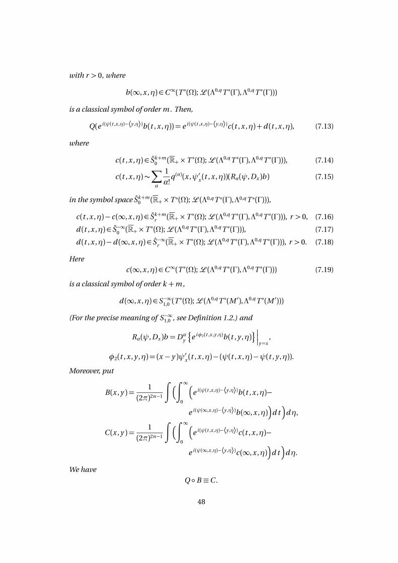
with r > 0, where
b (∞,x ,η)∈C∞(T ∗(Ω);L (Λ0,q T ∗(Γ),Λ0,q T ∗(Γ)))
is a classical symbol of order m . Then,
Q(e i (ψ(t ,x ,η)−⟨y ,η⟩)b (t ,x ,η)) = e i (ψ(t ,x ,η)−⟨y ,η⟩)c (t ,x ,η)+d (t ,x ,η), (7.13)
where
c (t ,x ,η)∈ Sk+m0 (R+×T ∗(Ω);L (Λ0,q T ∗(Γ),Λ0,q T ∗(Γ))), (7.14)
c (t ,x ,η)∼∑
α
1
α!q (α)(x ,ψ′x (t ,x ,η))(Rα(ψ, Dx )b ) (7.15)
in the symbol space Sk+m0 (R+×T ∗(Ω);L (Λ0,q T ∗(Γ),Λ0,q T ∗(Γ))),
c (t ,x ,η)− c (∞,x ,η)∈ Sk+mr (R+×T ∗(Ω);L (Λ0,q T ∗(Γ),Λ0,q T ∗(Γ))), r > 0, (7.16)
d (t ,x ,η)∈ S−∞0 (R+×T ∗(Ω);L (Λ0,q T ∗(Γ),Λ0,q T ∗(Γ))), (7.17)
d (t ,x ,η)−d (∞,x ,η)∈ S−∞r (R+×T ∗(Ω);L (Λ0,q T ∗(Γ),Λ0,q T ∗(Γ))), r > 0. (7.18)
Here
c (∞,x ,η)∈C∞(T ∗(Ω);L (Λ0,q T ∗(Γ),Λ0,q T ∗(Γ))) (7.19)
is a classical symbol of order k +m ,
d (∞,x ,η)∈S−∞1,0 (T∗(Ω);L (Λ0,q T ∗(M ′),Λ0,q T ∗(M ′)))
(For the precise meaning of S−∞1,0 , see Definition 1.2.) and
Rα(ψ, Dx )b =Dαy
¦
e iφ2(t ,x ,y ,η)b (t , y ,η)©
y=x,
φ2(t ,x , y ,η) = (x − y )ψ′x (t ,x ,η)− (ψ(t ,x ,η)−ψ(t , y ,η)).
Moreover, put
B (x , y ) =1
(2π)2n−1
∫
∫ ∞
0
e i (ψ(t ,x ,η)−⟨y ,η⟩)b (t ,x ,η)−
e i (ψ(∞,x ,η)−⟨y ,η⟩)b (∞,x ,η)
d t
dη,
C (x , y ) =1
(2π)2n−1
∫
∫ ∞
0
e i (ψ(t ,x ,η)−⟨y ,η⟩)c (t ,x ,η)−
e i (ψ(∞,x ,η)−⟨y ,η⟩)c (∞,x ,η)
d t
dη.
We have
Q B ≡C .
48
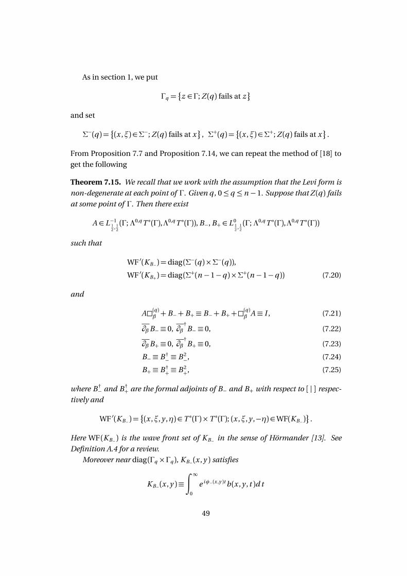
As in section 1, we put
Γq =
z ∈ Γ; Z (q ) fails at z
and set
Σ−(q ) =
(x ,ξ)∈Σ−; Z (q ) fails at x
, Σ+(q ) =
(x ,ξ)∈Σ+; Z (q ) fails at x
.
From Proposition 7.7 and Proposition 7.14, we can repeat the method of [18] to
get the following
Theorem 7.15. We recall that we work with the assumption that the Levi form is
non-degenerate at each point of Γ. Given q, 0≤q ≤ n −1. Suppose that Z (q ) fails
at some point of Γ. Then there exist
A ∈ L−112 , 1
2
(Γ; Λ0,q T ∗(Γ),Λ0,q T ∗(Γ)), B−, B+ ∈ L012 , 1
2
(Γ; Λ0,q T ∗(Γ),Λ0,q T ∗(Γ))
such that
WF ′(K B−) = diag (Σ−(q )×Σ−(q )),WF ′(K B+) = diag (Σ+(n −1−q )×Σ+(n −1−q )) (7.20)
and
A(q )β + B−+ B+ ≡ B−+ B++(q )β A ≡ I , (7.21)
∂βB− ≡ 0, ∂β†B− ≡ 0, (7.22)
∂βB+ ≡ 0, ∂β†B+ ≡ 0, (7.23)
B− ≡ B †− ≡ B 2
−, (7.24)
B+ ≡ B †+ ≡ B 2
+, (7.25)
where B †− and B †
+ are the formal adjoints of B− and B+ with respect to [ | ] respec-
tively and
WF ′(K B−) =
(x ,ξ, y ,η)∈ T ∗(Γ)×T ∗(Γ); (x ,ξ, y ,−η)∈WF(K B−)
.
Here WF (K B−) is the wave front set of K B− in the sense of Hörmander [13]. See
Definition A.4 for a review.
Moreover near diag (Γq ×Γq ), K B−(x , y ) satisfies
K B−(x , y )≡∫ ∞
0
e iφ−(x ,y )t b (x , y , t )d t
49
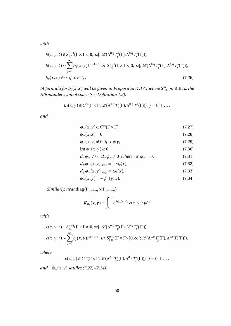
with
b (x , y , t )∈Sn−11,0 (Γ×Γ×]0,∞[;L (Λ0,q T ∗y (Γ),Λ
0,q T ∗x (Γ))),
b (x , y , t )∼∞∑
j=0
b j (x , y )t n−1−j in Sn−11,0 (Γ×Γ×]0,∞[;L (Λ0,q T ∗y (Γ),Λ
0,q T ∗x (Γ))),
b0(x ,x ) 6= 0 if x ∈ Γq , (7.26)
(A formula for b0(x ,x ) will be given in Proposition 7.17.) where Sm1,0, m ∈R, is the
Hörmander symbol space (see Definition 1.2),
b j (x , y )∈C∞(Γ×Γ;L (Λ0,q T ∗y (Γ),Λ0,q T ∗x (Γ))), j = 0, 1, . . . ,
and
φ−(x , y )∈C∞(Γ×Γ), (7.27)
φ−(x ,x ) = 0, (7.28)
φ−(x , y ) 6= 0 if x 6= y , (7.29)
Imφ−(x , y )≥ 0, (7.30)
d xφ− 6= 0, d yφ− 6= 0 where Imφ− = 0, (7.31)
d xφ−(x , y )|x=y =−ω0(x ), (7.32)
d yφ−(x , y )|x=y =ω0(x ), (7.33)
φ−(x , y ) =−φ−(y ,x ). (7.34)
Similarly, near diag (Γn−1−q ×Γn−1−q ),
K B+(x , y )≡∫ ∞
0
e iφ+(x ,y )t c (x , y , t )d t
with
c (x , y , t )∈Sn−11,0 (Γ×Γ×]0,∞[;L (Λ0,q T ∗y (Γ),Λ
0,q T ∗x (Γ))),
c (x , y , t )∼∞∑
j=0
c j (x , y )t n−1−j in Sn−11,0 (Γ×Γ×]0,∞[;L (Λ0,q T ∗y (Γ),Λ
0,q T ∗x (Γ))),
where
c (x , y )∈C∞(Γ×Γ;L (Λ0,q T ∗y (Γ),Λ0,q T ∗x (Γ))), j = 0, 1, . . . ,
and −φ+(x , y ) satifies (7.27)-(7.34).
50
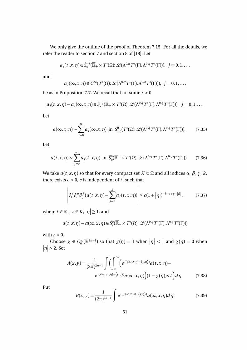
We only give the outline of the proof of Theorem 7.15. For all the details, we
refer the reader to section 7 and section 8 of [18]. Let
a j (t ,x ,η)∈ S−j0 (R+×T ∗(Ω);L (Λ0,q T ∗(Γ),Λ0,q T ∗(Γ))), j = 0, 1, . . . ,
and
a j (∞,x ,η)∈C∞(T ∗(Ω);L (Λ0,q T ∗(Γ),Λ0,q T ∗(Γ))), j = 0, 1, . . . ,
be as in Proposition 7.7. We recall that for some r > 0
a j (t ,x ,η)−a j (∞,x ,η)∈ S−jr (R+×T ∗(Ω);L (Λ0,q T ∗(Γ),Λ0,q T ∗(Γ))), j = 0, 1, . . . .
Let
a (∞,x ,η)∼∞∑
j=0
a j (∞,x ,η) in S01,0(T
∗(Ω);L (Λ0,q T ∗(Γ),Λ0,q T ∗(Γ))). (7.35)
Let
a (t ,x ,η)∼∞∑
j=0
a j (t ,x ,η) in S00(R+×T ∗(Ω);L (Λ0,q T ∗(Γ),Λ0,q T ∗(Γ))). (7.36)
We take a (t ,x ,η) so that for every compact set K ⊂ Ω and all indices α, β , γ, k ,
there exists c > 0, c is independent of t , such that
∂γ
t ∂α
x ∂βη (a (t ,x ,η)−
k∑
j=0
a j (t ,x ,η))
≤ c (1+
η
)−k−1+γ−|β |, (7.37)
where t ∈R+, x ∈ K ,
η
≥ 1, and
a (t ,x ,η)−a (∞,x ,η)∈ S0r (R+×T ∗(Ω);L (Λ0,q T ∗(Γ),Λ0,q T ∗(Γ)))
with r > 0.
Choose χ ∈ C∞0 (R2n−1) so that χ(η) = 1 when
η
< 1 and χ(η) = 0 when
η
> 2. Set
A(x , y ) =1
(2π)2n−1
∫
∫ ∞
0
e i (ψ(t ,x ,η)−⟨y ,η⟩)a (t ,x ,η)−
e i (ψ(∞,x ,η)−⟨y ,η⟩)a (∞,x ,η)
(1−χ(η))d t
dη. (7.38)
Put
B (x , y ) =1
(2π)2n−1
∫
e i (ψ(∞,x ,η)−⟨y ,η⟩)a (∞,x ,η)dη. (7.39)
51
Since a j (t ,x ,η), j = 0, 1, . . ., solve the transport equations (7.6), we can check that
B +(q )β A ≡ I ,
(q )β B ≡ 0.
From the global theory of Fourier integral operators (see Melin-Sjöstrand [23]),
we get
K B ≡ K B− +K B+ ,
wher K B− and K B+ are as in Theorem 7.15. By using a partition of unity we get the
global result.
Remark 7.16. For more properties of the phaseφ−(x , y ), see section 8 and section
9 of [18].
We can repeat the computation of the leading term of the Szegö projection
(see section 9 of [18]), to get the following
Proposition 7.17. Let p ∈ Γq , q = n−. Let
Z 1(x ), . . . ,Z n−1(x )
be an orthonormal frame of Λ1,0Tx (Γ), for which the Levi form is diagonalized at
p . Let e j (x ), j = 1, . . . , n − 1, denote the basis of Λ0,1T ∗x (Γ), which is dual to Z j (x ),j = 1, . . . , n − 1. Let λj (x ), j = 1, . . . , n − 1, be the eigenvalues of the Levi form Lx .
We assume that
λj (p )< 0 if 1≤ j ≤ n−.
Then
b0(p , p ) =1
2
λ1(p )
· · ·
λn−1(p )
π−n
j=n−∏
j=1
e j (p )∧e j (p )∧,∗,
where b0 is as in (7.26).
In section 8, we need the following
Proposition 7.18. Suppose that Z (q ) fails at some point of Γ. Let B− be as in
Theorem 7.15. Then,
γ∂ P B− ≡ 0. (7.40)
Proof. In view of Theorem 7.15, we know that
Tγ∂ P B− = ∂βB− ≡ 0, γ∂ f∗P B− = ∂β
†B− ≡ 0.
52
Combining this with (∂ ∂ f∗+ ∂ f
∗∂ )P = 0, we have
γ∂ f∗Pγ∂ P B− =−γ∂ Pγ∂ f
∗P B− ≡ 0
and
γ∂ f∗P(I −T )γ∂ P B− = γ∂ f
∗Pγ∂ P B−−γ∂ f
∗PTγ∂ P B− ≡ 0. (7.41)
Combining this with (4.6), we get
γ∂ f∗P(P∗P)−1(∂ r )∧Rγ∂ P B− ≡ 0.
Thus,
γ(∂ r )∧∂ f∗P(P∗P)−1(∂ r )∧Rγ∂ P B− ≡ 0. (7.42)
In view of Proposition 5.2, we know that
γ(∂ r )∧∂ f∗P(P∗P)−1 : C∞(Γ; I 0,q T ∗(M ′))→C∞(Γ; I 0,q T ∗(M ′))
is elliptic near Σ−, where I 0,q T ∗z (M′) is as in (5.17). Since
WF ′(K B−)⊂ diag (Σ−×Σ−),
we get
(∂ r )∧Rγ∂ P B− ≡ 0.
(See Proposition A.6 and Proposition A.7.) Thus, by (4.6),
(I −T )γ∂ P B− ≡ 0.
The proposition follows.
8 The Bergman projection
Given q , 0≤q ≤ n −1. In this section, we assume that Z (q ) fails at some point of
Γ and that Z (q−1) and Z (q+1) hold at each point of Γ. In view of Proposition 4.4,
we know that
Π(q ) : C∞(M ; Λ0,q T ∗(M ′))→D (q ).
Put
K = γΠ(q )P : C∞(Γ; Λ0,q T ∗(Γ))→C∞(Γ; Λ0,q T ∗(Γ)). (8.1)
Let K † be the formal adjoint of K with respect to [ | ]. That is,
K † :D ′(Γ; Λ0,q T ∗(Γ))→D ′(Γ; Λ0,q T ∗(Γ))
[K †u | v ] = [u | K v ], u ∈D ′(Γ; Λ0,q T ∗(Γ)), v ∈C∞(Γ; Λ0,q T ∗(Γ)).
53
Lemma 8.1. We have
K †v = K v,
v ∈C∞(Γ; Λ0,q T ∗(Γ)).
Proof. For u , v ∈C∞(Γ; Λ0,q T ∗(Γ)), we have
[K u | v ] = [γΠ(q )Pu | v ]= (Π(q )Pu | Pv )M
= (Pu | Π(q )Pv )M
= [u | K v ].
Thus,
K †v = K v.
The lemma follows.
We can extend K to
D ′(Γ; Λ0,q T ∗(Γ))→D ′(Γ; Λ0,q T ∗(Γ))
by the following formula
[K u | v ] = [u | K †v ], u ∈D ′(Γ; Λ0,q T ∗(Γ)), v ∈C∞(Γ; Λ0,q T ∗(Γ)).
Lemma 8.2. Let u ∈D ′(Γ; Λ0,q T ∗(Γ)). We have
WF (K u )⊂Σ−.
Proof. Let u ∈D ′(Γ; Λ0,q T ∗(Γ)). We have
(γ(∂ r )∧,∗∂ P)(K u ) = 0.
In view of Proposition 5.1, we know that γ(∂ r )∧,∗∂ P is elliptic outside Σ−. The
lemma follows.
Lemma 8.3. Let B− be as in Theorem 7.15. We have
B−K ≡ K B− ≡ K .
Proof. Let A, B− and B+ be as in Theorem 7.15. In view of Theorem 7.15, we have
B−+ B++A(q )β ≡ I .
54
We may replace B+ by I −A(q )β − B− and get
B−+ B++A(q )β = I .
It is easy to see that
(q )β K = 0.
Thus,
K = (B−+ B++A(q )β )K = (B−+ B+)K . (8.2)
Let u ∈D ′(Γ; Λ0,q T ∗(Γ)). From Lemma 8.2, we know that
WF (K u )⊂Σ−.
Note that
WF ′(K B+)⊂ diag (Σ+×Σ+).
Thus,
B+K u ∈C∞,
so B+K is smoothing and
(B−+ B+)K ≡ B−K .
From this and (8.2), we get
K ≡ B−K
and
K = K † ≡ K † B †− ≡ K B−.
The lemma follows.
We pause and introduce some notations. Let X and Y be C∞ vector bundles
over M ′ and Γ respectively. Let
C , D : C∞(Γ; Y )→D ′(M ; X )
with distribution kernels
KC (z , y ), KD(z , y )∈D ′(M ×Γ;L (Yy , Xz )).
We write
C ≡D mod C∞(M ×Γ)
if
KC (z , y ) = KD(z , y )+ F (z , y ),
where F (z , y )∈C∞(M ×Γ;L (Yy , Xz )).
55
Lemma 8.4. We have
Π(q )P B− ≡Π(q )P modC∞(M ×Γ). (8.3)
Proof. From Lemma 8.3, we have
K = γΠ(q )P ≡ K B− = γΠ(q )P B−.
Thus,
Π(q )P = PγΠ(q )P ≡ PγΠ(q )P B− modC∞(M ×Γ).
We get (8.3).
Put
Q = P B−T (P∗P)−1P∗ : C∞(M ; Λ0,q T ∗(M ′))→C∞(M ; Λ0,q T ∗(M ′)), (8.4)
where T is as in (4.5).
Proposition 8.5. We have
Q ≡Π(q ) modC∞(M ×M ).
Proof. We have
Π(q )Q =Π(q )P B−T (P∗P)−1P∗ ≡Π(q )PT (P∗P)−1P∗ modC∞(M ×M ). (8.5)
Here we used (8.3). From (8.5) and the first part of (4.10), we get
Π(q )Q ≡Π(q ) modC∞(M ×M ). (8.6)
From Theorem 3.7, we have
Π(q )Q = (I − ∂∗N (q+1)∂ − ∂ N (q−1)∂
∗)Q ,
where N (q+1) and N (q−1) are as in Theorem 3.6. From (7.40), (7.22) and Lemma 6.2,
we see that
∂Q ≡ 0, ∂∗Q ≡ 0 modC∞(M ×M ).
Thus,
Π(q )Q = (I − ∂∗N (q+1)∂ − ∂ N (q−1)∂
∗)Q ≡Q modC∞(M ×M ).
From this and (8.6), the proposition follows.
56
Let x = (x1, . . . ,x2n−1) be a system of local coordinates on Γ and extend
x1, . . . ,x2n−1
to real smooth functions in some neighborhood of Γ. We write
(ξ1, . . . ,ξ2n−1,θ )
to denote the dual variables of (x1, . . . ,x2n−1, r ). We write
z = (x1, . . . ,x2n−1, r ), x = (x1, . . . ,x2n−1, 0)
and
ξ= (ξ1, . . . ,ξ2n−1), ζ= (ξ1, . . . ,ξ2n−1,θ ).
Until further notice, we work with the local coordinates z = (x , r ) defined on
some neighborhood of p ∈ Γ.
We represent the Riemannian metric on T (M ′) by
h =2n∑
j ,k=1
h j ,k (z )d x j ⊗d xk , d x2n = d r,
where h j ,k (z ) = hk ,j (z ), j , k = 1, . . . , n , and
h j ,k (z )
1≤j ,k≤2nis positive definite at
each point of M ′. Put
h j ,k (z )−1
1≤j ,k≤2n=
h j ,k (z )
1≤j ,k≤2n.
It is well-known (see page 99 of [25]) that
(q )f =−1
2
h2n ,2n (z )∂ 2
∂ r 2+2
2n−1∑
j=1
h2n ,j (z )∂ 2
∂ r ∂ x j+T (r )
+lower order terms, (8.7)
where
T (r ) =2n−1∑
j ,k=1
h j ,k (z )∂ 2
∂ x j ∂ xk. (8.8)
Note that
T (0) =4Γ+ lower order terms (8.9)
and
h2n ,2n (x ) = 1, h2n ,j (x ) = 0, j = 1, . . . , 2n −1. (8.10)
We let the full symbol of (q )f be:
full symbol of (q )f =2∑
j=0
qj (z ,ζ)
where qj (z ,ζ) is a homogeneous polynomial of order 2− j in ζ. We have the
following
57
Proposition 8.6. Let φ− ∈C∞(Γ×Γ) be as in Theorem 7.15. Then, in some neigh-
borhood U of diag (Γq ×Γq ) in M ′×M ′, there exists a smooth function
eφ(z , y )∈C∞((M ×Γ)⋂
U )
such that
eφ(x , y ) =φ−(x , y ),
Im eφ ≥ 0,
d zeφ 6= 0, d yeφ 6= 0 where Im eφ = 0,
Im eφ > 0 if r 6= 0, (8.11)
and
q0(z , eφ′z )
vanishes to infinite order on r = 0. We write ∂∂ r (z ) to denote ∂
∂ racting in the z
variables. We have
∂
∂ r (z )eφ(z , y )|r=0 =−i
p
−σ4Γ(x , (φ−)′x ) (8.12)
in some neighborhood of x = y , where
Rep
−σ4Γ(x , (φ−)′x )> 0.
Proof. From (8.7) and (8.8), we have
q0(z ,ζ) =1
2h2n ,2n (z )θ 2+
2n−1∑
j=1
h2n ,j (z )θξj + g (z ,ξ),
g (x ,ξ) =−1
2σ4Γ , (8.13)
where g (z ,ξ) is the principal symbol of − 12
T (r ).We consider the Taylor expansion of q0(z ,ζ)with respect to r ,
q0(z ,ζ) =1
2θ 2−
1
2σ4Γ +
∞∑
j=1
g j (x ,ξ)r j +∞∑
j=1
s j (x ,ζ)θ r j . (8.14)
We introduce the Taylor expansion of eφ(z , y )with respect to r ,
eφ(z , y ) =φ−(x , y )+∞∑
1
φj (x , y )r j .
Let
φ1(x , y ) =−ip
−σ4Γ(x , (φ−)′x ).
58
Since (φ−)′x |x=y = −ω0(x ) is real, we choose the branch ofp
−σ4Γ(x , (φ−)′x ) so
that
Rep
−σ4Γ(x , (φ−)′x )> 0
in some neighborhood of x = y , r = 0. Put
eφ1(z , y ) =φ−(x , y )+ rφ1(x , y ).
We have
q0(z , ( eφ1)′z ) =O(r ).
Similarly, we can findφ2(x , y ) so that
q0(z , ( eφ2)′z ) =O(r 2),
where eφ2(z , y ) =φ−(x , y ) + rφ1(x , y ) + r 2φ2(x , y ). Continuing in this way we get
the phase eφ(z , y ) such that
eφ(x , y ) =φ−(x , y )
and
q0(z , eφ′z )
vanishes to infinite order on r = 0. The proposition follows.
Remark 8.7. Let eφ(z , y ) be as in Proposition 8.6 and let
d (z , y , t )∈Sm1,0(M ×Γ×]0,∞[;L (Λ0,q T ∗y (M
′),Λ0,q T ∗z (M′)))
with support in some neighborhood of diag (Γq × Γq ). (For the meaning of the
space Sm1,0(M ×Γ×]0,∞[;L (Λ0,q T ∗y (M
′),Λ0,q T ∗z (M′))), see Definition 1.2.) Choose
a cut-off function χ(t ) ∈ C∞(R) so that χ(t ) = 1 when |t | < 1 and χ(t ) = 0 when
|t |> 2. For all u ∈C∞(Γ; Λ0,q T ∗(M ′)), set
(Dεu )(z ) =
∫ ∫ ∞
0
e i eφ(z ,y )t d (z , y , t )χ(εt )u (y )d t d y .
Since Im eφ ≥ 0 and d yeφ 6= 0 where Im eφ = 0, we can integrate by parts in y , t and
obtain
limε→0(Dεu )(z )∈C∞(M ; Λ0,q T ∗(M ′)).
This means that
D = limε→0
Dε : C∞(Γ; Λ0,q T ∗(M ′))→C∞(M ; Λ0,q T ∗(M ′))
is continuous. Formally,
D(z , y ) =
∫ ∞
0
e i eφ(z ,y )t d (z , y , t )d t .
59
Proposition 8.8. Let
B−(x , y ) =
∫ ∞
0
e iφ−(x ,y )t b (x , y , t )d t
be as in Theorem 7.15. We have
P B−(z , y )≡∫ ∞
0
e i eφ(z ,y )teb (z , y , t )d t modC∞(M ×Γ)
witheb (z , y , t )∈Sn−1
1,0 (M ×Γ×]0,∞[;L (Λ0,q T ∗y (M′),Λ0,q T ∗z (M
′))),
eb (z , y , t )∼∞∑
j=0
eb j (z , y )t n−1−j
in the space Sn−11,0 (M ×Γ×]0,∞[;L (Λ0,q T ∗y (M
′),Λ0,q T ∗z (M′))), where
eb j (z , y )∈C∞(M ×Γ;L (Λ0,q T ∗y (M′),Λ0,q T ∗z (M
′))), j = 0, 1, . . . .
Proof. Put
b (x , y , t )∼∞∑
j=0
b j (x , y )t n−1−j
and formally set
eb (z , y , t )∼∞∑
j=0
eb j (z , y )t n−1−j .
We notice that
B−(x , y )∈C∞(Γ×Γ \diag (Γq ×Γq );L (Λ0,q T ∗y (Γ),Λ0,q T ∗z (Γ))).
For simplicity, we may assume that b (x , y , t ) = 0 outside some small neighbor-
hood of diag (Γq ×Γq ). Put
(q )f (eb (z , y , t )e i eφt ) = ec (z , y , t )e i eφt .
From (7.29) and (8.11), we know that near diag (Γq × Γq ), eφ(z , y ) = 0 if and only
if x = y , r = 0. From this observation, we see that if ec (z , y , t ) vanishes to infinite
order on diag (Γq ×Γq )×R+, we can integrate by parts and obtain
limε→0
∫ ∞
0
e i eφtec (z , y , t )χ(εt )d t ≡ 0 modC∞(M ×Γ),
60
where χ(t ) is as in Remark 8.7. Thus, we only need to consider the Taylor ex-
pansion of eb (z , y , t ) on x = y , r = 0. We introduce the asymptotic expansion of
(q )f (eb e i eφt ). Setting
(q )f (eb e i eφt )∼ 0
and regrouping the terms according to the degree of homogeneity. We obtain the
transport equations¨
T (z , y ,∂z )eb0(z , y ) = 0
T (z , y ,∂z )eb j (z , y )+ l j (z , y ,eb0(z , y ), . . . ,eb j−1(z , y )) = 0, j = 1, 2, . . . .(8.15)
Here
T (z , y ,∂z ) =−i2n−1∑
j=1
∂ q0
∂ ξj(z , eφ′z )
∂
∂ x j− i∂ q0
∂ θ(z , eφ′z )
∂
∂ r
+R(z , y ),
where
R(z , y ) =q1(z , eφ′z )+1
2i
2n∑
j ,k=1
∂ 2q0(z , eφ′z )∂ ξj ∂ ξk
∂ 2eφ
∂ x j ∂ xk, x2n = r, ξ2n = θ ,
and l j is a linear differential operator acting on eb0(z , y ), . . . ,eb j−1(z , y ).We introduce the Taylor expansion of eb0(z , y )with respect to r ,
eb0(z , y ) =b0(x , y )+∞∑
1
b j0(x , y )r j .
Since∂ q0
∂ θ|r=0 = θ
andeφ′r |r=0 =−ip
−σ4Γ(x , (φ−)′x ),
we have∂ q0
∂ θ(z , eφ′z )|r=0 6= 0
in some neighborhood of x = y . Thus, we can find b 10(x , y )r such that
T (z , y ,∂z )(b0(x , y )+b 10(x , y )r ) =O(|r |)
in some neighborhood of r = 0, x = y . We can repeat the procedure above to find
b 20(x , y ) such that
T (z , y ,∂z )(b0(x , y )+2∑
k=1
b k0 (x , y )r k ) =O(|r |2)
61
in some neighborhood of r = 0, x = y . Continuing in this way we solve the first
transport equation to infinite order at r = 0, x = y .
For the second transport equation, we can repeat the method above to solve
the second transport equation to infinite order at r = 0, x = y . Continuing in this
way we solve (8.15) to infinite order at r = 0, x = y .
Put
eB (z , y ) =
∫ ∞
0
e i eφ(z ,y )teb (z , y , t )d t .
From the construction above, we see that
(q )feB ≡ 0 modC∞(M ×Γ), γ eB ≡ B−. (8.16)
It is well-known (see chapter XX of [14]) that there exists
G : C∞(M ; Λ0,q T ∗(M ′))→C∞(M ; Λ0,q T ∗(M ′))
such that
G(q )f +Pγ= I on C∞(M ; Λ0,q T ∗(M ′)). (8.17)
From this and (8.16), we have
eB = (G(q )f +Pγ) eB ≡ P B− modC∞(M ×Γ).
The proposition follows.
From Proposition 8.8, we have
C (z , y ) := P B−T (P∗P)−1(z , y )≡∫ ∞
0
e i eφ(z ,y )t c (z , y , t )d t modC∞(M ×Γ)
with
c (z , y , t )∈Sn1,0(M ×Γ×]0,∞[;L (Λ0,q T ∗y (M
′),Λ0,q T ∗z (M′))),
c (z , y , t )∼∞∑
j=0
c j (z , y )t n−j
in the space Sn1,0(M ×Γ×]0,∞[;L (Λ0,q T ∗y (M
′),Λ0,q T ∗z (M′))). Let
C ∗ : C∞(M ; Λ0,q T ∗(M ′))→D ′(Γ; Λ0,q T ∗(M ′))
be the operator defined by
(C ∗u | v )Γ = (u | C v )M , u ∈C∞(M ; Λ0,q T ∗(M ′)), v ∈C∞(Γ; Λ0,q T ∗(M ′)).
62
The distribution kernel of C ∗ is
C ∗(y , z )≡∫ ∞
0
e−i eφ(z ,y )t c ∗(y , z , t )d t modC∞(Γ×M ) (8.18)
where
c ∗(y , z , t )∈Sn1,0(Γ×M×]0,∞[;L (Λ0,q T ∗z (M
′),Λ0,q T ∗y (M′))),
(c ∗(y , z , t )µ | ν ) = (µ | c (y , z , t )ν ), µ∈Λ0,q T ∗z (M′), ν ∈Λ0,q T ∗y (M
′),
c ∗(y , z , t )∼∞∑
j=0
c ∗j (y , z )t n−j
in Sn1,0(Γ×M×]0,∞[;L (Λ0,q T ∗z (M
′),Λ0,q T ∗y (M′))). The oscillatory integral (8.18) is
defined as follows: Let u ∈C∞(M ; Λ0,q T ∗(M ′)). Set
(C ∗εu )(y ) =
∫ ∫ ∞
0
e−i eφ(z ,y )t c ∗(y , z , t )χ(εt )u (z )d t d z ,
where χ is as in Remark 8.7. Since d xeφ 6= 0 where Im eφ = 0, we can integrate by
parts in x and t and obtain
limε→0(C ∗εu )(y )∈C∞(Γ; Λ0,q T ∗(M ′)).
This means that
C ∗ = limε→0
C ∗ε : C∞(M ; Λ0,q T ∗(M ′))→C∞(Γ; Λ0,q T ∗(M ′))
is continuous.
We can repeat the proof of Proposition 8.6 to find
φ(z , w )∈C∞(M ×M )
such that
φ(z , y ) = eφ(z , y ),
Imφ ≥ 0,
Imφ > 0 if (z , w ) /∈ Γ×Γ
and
q0(w ,−φ′w )
vanishes to infinite order on r = 0. Since φ−(x , y ) = −φ−(y ,x ), we can take
φ(z , w ) so that
φ(z , w ) =−φ(w , z ).
63
As in the proof of Proposition 8.8, we can find
a ∗(w , z , t )∈Sn1,0(M ×M × [0,∞[;L (Λ0,q T ∗z (M
′),Λ0,q T ∗w (M′))),
a ∗(w , z , t )∼∞∑
j=0
a ∗j (w , z )t n−j
in Sn1,0(M ×M×]0,∞[;L (Λ0,q T ∗z (M
′),Λ0,q T ∗w (M′))), such that
a ∗(y , z , t ) = c ∗(y , z , t )
and
(q )f (a∗(w , z , t )e−iφ(z ,w )t )
vanishes to infinite order on diag (Γq ×Γq )×R+. From (8.17), we have
PC ∗(w , z )≡∫ ∞
0
e−iφ(z ,w )t a ∗(w , z , t )d t modC∞(M ×M ).
Thus,
C P∗(z , w ) = P B−T (P∗P)−1P∗(z , w )≡∫ ∞
0
e iφ(z ,w )t a (z , w , t )d t modC∞(M ×M ),
a (z , w , t )∈Sn1,0(M ×M × [0,∞[;L (Λ0,q T ∗w (M
′),Λ0,q T ∗z (M′))),
a (z , w , t )∼∞∑
j=0
a j (z , w )t n−j
in the space Sn1,0(M×M×]0,∞[;L (Λ0,q T ∗w (M
′),Λ0,q T ∗z (M′))). From this and Propo-
sition 8.5, we get the main result of this work
Theorem 8.9. Given q, 0 ≤ q ≤ n − 1. Suppose that Z (q ) fails at some point of Γand that Z (q −1) and Z (q +1) hold at each point of Γ. Then
KΠ(q )(z , w )∈C∞(M ×M \diag (Γq ×Γq );L (Λ0,q T ∗w (M′),Λ0,q T ∗z (M
′))).
Moreover, in a neighborhood U of diag (Γq ×Γq ), KΠ(q )(z , w ) satisfies
KΠ(q )(z , w )≡∫ ∞
0
e iφ(z ,w )t a (z , w , t )d t mod C∞(U⋂
(M ×M )) (8.19)
with
a (z , w , t )∈Sn1,0(U⋂
(M ×M )×]0,∞[;L (Λ0,q T ∗w (M′),Λ0,q T ∗z (M
′))),
64
a (z , w , t )∼∞∑
j=0
a j (z , w )t n−j
in the space Sn1,0(U⋂
(M ×M )×]0,∞[;L (Λ0,q T ∗w (M′),Λ0,q T ∗z (M
′))),
a 0(z , z ) 6= 0, z ∈ Γq ,
where
a j (z , w )∈C∞(U⋂
(M ×M );L (Λ0,q T ∗w (M′),Λ0,q T ∗z (M
′))), j = 0, 1, . . . ,
and
φ(z , w )∈C∞(U⋂
(M ×M )), (8.20)
φ(z , z ) = 0, z ∈ Γq , (8.21)
φ(z , w ) 6= 0 if (z , w ) /∈ diag (Γq ×Γq ), (8.22)
Imφ ≥ 0, (8.23)
Imφ(z , w )> 0 if (z , w ) /∈ Γ×Γ, (8.24)
φ(z , w ) =−φ(w , z ). (8.25)
For p ∈ Γq , we have
σ(q )f(z , d zφ(z , w )) vanishes to infinite order at z = p ,
(z , w ) is in some neighborhood of (p , p ) in M ′. (8.26)
For z =w , z ∈ Γq , we have
d zφ =−ω0− i d r,
d wφ =ω0− i d r.
As before, we put
B−(x , y )≡∫ ∞
0
e iφ−(x ,y )t b (x , y , t )d t ,
b (x , y , t )∼∞∑
j=0
b j (x , y )t n−1−j ,
and
KΠ(q )(z , w )≡∫ ∞
0
e iφ(z ,w )t a (z , w , t )d t
a (z , w , t )∼∞∑
j=0
a j (z , w )t n−j .
65
Since Π(q ) ≡ P B−T (P∗P)−1P∗,
(P∗P)−1 = 2p
−4Γ+ lower order terms
and
T = 2(∂ r )∧,∗(∂ r )∧+ lower order terms,
we have
a 0(x ,x ) = 2σp−4Γ(x , (φ−)′y (x ,x ))b0(x ,x )2(∂ r (x ))∧,∗(∂ r (x ))∧, x ∈ Γ.
Since (φ−)′y (x ,x ) =ω0(x ) and ‖ω0‖= 1 on Γ, it follows that
a 0(x ,x ) = 4b0(x ,x )(∂ r (x ))∧,∗(∂ r (x ))∧. (8.27)
From this and Proposition 7.17, we get the following
Proposition 8.10. Under the assumptions of Theorem 8.9, let p ∈ Γq , q = n−. Let
Z 1(z ), . . . ,Z n−1(z )
be an orthonormal frame of Λ1,0Tz (Γ), z ∈ Γ, for which the Levi form is diagonal-
ized at p . Let e j (z ), j = 1, . . . , n − 1 denote the basis of Λ0,1T ∗z (Γ), z ∈ Γ, which is
dual to Z j (z ), j = 1, . . . , n − 1. Let λj (z ), j = 1, . . . , n − 1 be the eigenvalues of the
Levi form L z , z ∈ Γ. We assume that
λj (p )< 0 if 1≤ j ≤ n−.
Then
a 0(p , p ) =
λ1(p )
· · ·
λn−1(p )
π−n 2
j=n−∏
j=1
e j (p )∧e ∧,∗j (p )
(∂ r (p ))∧,∗(∂ r (p ))∧. (8.28)
9 Examples
The aim of this section is to illustrate the results in some simple examples. First,
we will show that when M ′ is Kähler (see below), then F (q ) is injective for any q ,
0≤q ≤ n . We recall that F (q ) is defined by (1.9).
As before, let g =∑n
j ,k=1 g j ,k d z j ⊗d z k be the Hermitian metric on Λ1,0T (M ′)and let
ω= in∑
j ,k=1
g j ,k d z j ∧d z k
66
be the associated real (1, 1)-form. We call g a Kähler metric if dω = 0. ω is
then called its Kähler form. A complex manifold endowed with a Kähler metric is
called a Kähler manifold.
Let
∂ : C∞(M ′; Λp ,q T ∗(M ′))→C∞(M ′; Λp+1,q T ∗(M ′))
be the part of the exterior differential operator which maps forms of type (p ,q )to forms of type (p +1,q ) and we denote by
∂ ∗f : C∞(M ′; Λp+1,q T ∗(M ′))→C∞(M ′; Λp ,q T ∗(M ′))
the formal adjoint of ∂ . The following is well-known (see page 113 of Morrow
and Kodaira [25])
Proposition 9.1. If M ′ is Kähler, then
∂ ∂ ∗f + ∂∗
f ∂ = ∂ ∂ f∗+ ∂ f
∗∂
on the space C∞(M ′; Λp ,q T ∗(M ′)), 0≤ p ,q ≤ n.
Note that
∂ ∗f u = 0, u ∈C∞(M ′; Λ0,q T ∗(M ′)), ∂ u = 0, u ∈C∞(M ′; Λp ,n T ∗(M ′))
and
∂ f∗u = 0, u ∈C∞(M ′; Λp ,0T ∗(M ′)), ∂ u = 0, u ∈C∞(M ′; Λn ,q T ∗(M ′)).
Now, we assume that M ′ is Kähler. We claim that F (q ) is injective, for any q ,
0 ≤ q ≤ n . Given q , 0 ≤ q ≤ n . Let u ∈ Ker F (q ). Then, u ∈ C∞(M ; Λ0,q T ∗(M ′)),∂ u = 0, ∂ f
∗u = 0 and γu = 0. From Proposition 9.1, we can check that
∂ u = 0.
We work with local coordinates z = (z 1, . . . , z n ) defined on some neighborhood of
p ∈ Γ. We write
u =∑
J
u J d z J , J = (j1, . . . , jq ), 1≤ j1 < j2 < · · ·< jq ≤ n .
Since ∂ u = 0, for any J ,∂ u J
∂ z j= 0, j = 1, . . . , n .
u J is holomorphic and γu J = 0. Thus, u J = 0 and consequently u = 0. We have
proved the claim.
67
9.1 Complex projective space
For a point (ξ0,ξ1, . . . ,ξn )∈Cn+1 \ (0, 0, . . . , 0),
ξ= (λξ0,λξ1, . . . ,λξn ); λ∈C
is a complex line through 0 = (0, 0, . . . , 0). The collection of all complex lines
through 0 is called the n-dimensional complex projective space and denoted by
CPn . A point ξ of CPn represents a complex line
ξ= (λξ0, . . . ,λξn ); λ∈C .
ξ0, . . . ,ξn are called the homogeneous coordinates of ξ ∈ CPn and denoted by
ξ= (ξ0, . . . ,ξn ). The equality
(ξ′0, . . . ,ξ′n ) = (ξ0, . . . ,ξn )
means that ξ′0 =λξ0, . . . ,ξ′n =λξn for some λ 6= 0, λ∈C. Put
Uj =¦
ξ= (ξ0, . . . ,ξn )∈CPn ; ξj 6= 0©
. (9.1)
ξ∈Uj is represented as
ξ= (ξ0
ξj, . . . ,
ξj−1
ξj, 1,ξj+1
ξj, . . . ,
ξn
ξj).
The map
z j : ξ→ z j (ξ) = (ξ0
ξj, . . . ,
ξj−1
ξj,ξj+1
ξj, . . . ,
ξn
ξj)
= (z 1, . . . , z n ) (9.2)
gives local coordinates on Uj whereUj = z j (Uj ) =Cn . If
z = (z 1, . . . , z n )∈ z j (Uj
⋂
Uk ), j > k ,
then z k 6= 0. The coordinates transformations
τk ,j : z j (Uj
⋂
Uk )→ z k (Uj
⋂
Uk ),
(z 1, . . . , z n )→ (z 1
z k, . . . ,
z k−1
z k,
z k+1
z k, . . . ,
z j−1
z k,
1
z k,
z j+1
z k, . . . ,
z n
z k) (9.3)
are biholomorphic. CPn is a complex manifold obtained by glueing the (n + 1)-copies of Cn via the isomorphisms (9.3).
68
On Uν , put
a ν (ξ) =1
|ξν |2(|ξ0|2+ · · ·+ |ξn |2), ξ= (ξ0, . . . ,ξn ). (9.4)
Now, we work with local coordinates
z = (z 1, . . . , z n ) = (ξ0
ξν, . . . ,
ξν−1
ξν,ξν+1
ξν, . . . ,
ξn
ξν) (9.5)
defined on Uν . Then,
a ν (z ) = 1+n∑
j=1
z j
2.
We can check that
∂ ∂ log a ν (z ) =n∑
j ,k=1
g j ,k d z j ∧d z k ,
where
g j ,k =1
a ν (z )2(a ν (z )δj ,k − z j z k ). (9.6)
Here δj ,k = 0 if j 6= k , δj ,k = 1 if j = k . The Hermitian metric∑n
j ,k=1 g j ,k d z j ⊗d z k
is easily seen to be positive definite. Note that
a ν (z ) =
eν ,µ(z )
2aµ(z ), eν ,µ =
ξµ
ξνon Uν
⋂
Uµ.
eν ,µ is a non-vanishing holomorphic function. Hence
∂ ∂ log a ν (z ) = ∂ ∂ log aµ(z ) on Uν
⋂
Uµ.
Thus,∑n
j ,k=1 g j ,k d z j ⊗d z k gives a Hermitian metric on CPn . Its associated real
(1, 1)-form is given by
ω= i∂ ∂ log a ν (z )
= i d ∂ log a ν (z ) on Uν ,
since d = ∂ +∂ . Therefore dω= 0 and∑n
j ,k=1 g j ,k d z j ⊗d z k is a Kähler metric on
CPn .
Now, we fix the Hermitian metric above onCPn . Let
r (ξ) =1
|ξ|2(−λ0 |ξ0|2−λ1 |ξ1|2− · · ·−λk0
ξk0
2+λk0+1
ξk0+1
2+ · · ·+λn |ξn |2),
where |ξ|2 = |ξ0|2+ · · ·+ |ξn |2, λj > 0, j = 0, 1, . . . , n . Put
Γ= ξ∈CPn ; r (ξ) = 0 , M = ξ∈CPn ; r (ξ)< 0 .
It is easy to see that d r 6= 0 at each point of Γ.
69
Lemma 9.2. Γ is connected.
Proof. Let ξ= (ξ0, . . . ,ξn ), ξ′ = (ξ′0, . . . ,ξ′n )∈ Γ. We have
λ0 |ξ0|2+λ1 |ξ1|2+ · · ·+λk0
ξk0
2=λk0+1
ξk0+1
2+ · · ·+λn |ξn |2
and
λ0
ξ′0
2+λ1
ξ′1
2+ · · ·+λk0
ξ′k0
2
=λk0+1
ξ′k0+1
2
+ · · ·+λn
ξ′n
2.
Since C is connected, we can find continuous curves
c j (t ) : [0, 1]→C, j = 0, 1, . . . , n ,
such that
c j (0) = ξj , c j (1) = ξ′j , j = 0, 1, . . . , n .
Put
d (t )2 =λ0 |c0(t )|2+ · · ·+λk0
ck0(t )
2
λk0+1
ck0+1(t )
2+ · · ·+λn |cn (t )|2
.
Then,
d (0) = d (1) = 1.
Put
c (t ) : [0, 1]→ Γt → (c0(t ), . . . , ck0(t ), d (t )ck0+1(t ), . . . , d (t )cn (t )).
Then,
c (0) = ξ, c (1) = ξ′.
The lemma follows.
Now, we work with local coordinates
(z 1, . . . , z n ) = (ξ1
ξ0,ξ2
ξ0, . . . ,
ξn
ξ0)
defined on U0. Then,
r (z ) =1
a 0(z )(−λ0−λ1 |z 1|2− · · ·−λk0
z k0
2+λk0+1
z k0+1
2+ · · ·+λn |z n |2),
where a 0(z ) = 1+∑n
j=1
z j
2. Let U =∑n
k=1 u k∂∂ z k
, V =∑n
j=1 v j∂∂ z j∈ Λ1,0Tp (Γ),
p ∈ Γ. From (2.33), we have
L p (U , V ) =1
a 0(p )
d r (p )
(−k0∑
j=1
λj u j w j +n∑
j=k0+1
λj u j w j ). (9.7)
70
We notice that U =∑n
j=1 u j∂∂ z j∈Λ1,0Tp (Γ) if and only if
n∑
j=1
∂ r
∂ z ju j =−
k0∑
j=1
λj z j u j +n∑
k0+1
λj z j u j = 0, p = (z 1, . . . , z n ). (9.8)
Proposition 9.3. The Levi form is non-degenerate at each point of Γ and we have
Γ=Γk0 . That is, the number of negative eigenvalues of the Levi form is k0.
Proof. Let p = (z 1, . . . , z n ) ∈ Γ and let U =∑n
j=1 u j∂∂ z j∈ Λ1,0Tp (Γ). If L p (U , W ) = 0
for all W ∈Λ1,0Tp (Γ), from (9.7), (9.8), we see that
(u 1, . . . , u n ) = c (z 1, . . . , z n ), c ∈C.
From (9.8), we have
−k0∑
j=1
λj z j u j +n∑
k0+1
λj z j u j = c (−k0∑
j=1
λj
z j
2+
n∑
k0+1
λj
z j
2) =λ0c = 0.
Thus, c = 0 and consequently the Levi form is non-degenerate at p .
We compute the signature of the Levi form at
z 0 = (0, . . . , 0,
r
λ0
λn)∈ Γ.
From (9.8), we have
Λ1,0Tz 0(Γ) =
n−1∑
j=1
u j∂
∂ z j; u j ∈C, j = 1, . . . , n −1
.
For U =∑n−1
k=1 u k∂∂ z k
, V =∑n−1
j=1 v j∂∂ z j∈Λ1,0Tz 0(Γ), we have
L z 0(U , V ) =1
a 0(z 0)‖d r (z 0)‖(−
k0∑
j=1
λj u j w j +n−1∑
j=k0+1
λj u j w j ).
Thus, the number of negative eigenvalues of L z 0 is k0. The proposition follows.
From Theorem 1.3, we know that if q 6= k0, then
KΠ(q ) ∈C∞(M ×M ;L (Λ0,q T ∗w (M′),Λ0,q T ∗z (M
′))).
71
If q = k0, then Z (q − 1) and Z (q + 1) hold at each point of Γ. From Theorem 1.3,
we have
KΠ(q ) ≡∫ ∞
0
e iφ(z ,w )t b (z , w , t )d t modC∞(M ×M )
with
b (z , w , t )∈Sn1,0(M ×M×]0,∞[;L (Λ0,q T ∗w (M
′),Λ0,q T ∗z (M′))),
b (z , w , t )∼∞∑
j=0
b j (z , w )t n−j
in the space Sn1,0(M ×M×]0,∞[;L (Λ0,q T ∗w (M
′),Λ0,q T ∗z (M′))),
b0(z , z ) 6= 0, z ∈ Γ.
We continue to work with local coordinates
(z 1, . . . , z n ) = (ξ1
ξ0,ξ2
ξ0, . . . ,
ξn
ξ0)
defined on U0. We study the leading term of KΠ(q ) at
z 0 = (0, . . . , 0,
r
λ0
λn).
It is straight forward to see that
g (z 0) =n−1∑
j=1
1
a 0(z 0)d z j ⊗d z j +
1
a 0(z 0)2d z n ⊗d z n ,
‖d r (z 0)‖2 = 2λnλ0
and
∂ r (z 0) =1
a 0(z 0)
p
λ0λn d z n ,
where
a 0(z 0) =λn +λ0
λn.
We can check thatp
a 0(z 0)∂
∂ z 1, . . . ,p
a 0(z 0)∂
∂ z n−1
is an orthonormal frame of Λ0,1Tz 0(Γ) and the eigenvalues of L z 0 are
−1
‖d r (z 0)‖λ1, . . . ,−
1
‖d r (z 0)‖λk0 ,
1
‖d r (z 0)‖λk0+1, . . . ,
1
‖d r (z 0)‖λn .
72
Put
e1 =1p
a 0(z 0)d z 1, . . . , en−1 =
1p
a 0(z 0)d z n−1.
From Proposition 1.7, we have
b0(z 0, z 0) = 2 |λ1| · · · |λn−1| |d r (z 0)|−(n+1)π−n
k0∏
j=1
e ∧j e ∧,∗j
(∂ r (z 0))∧,∗(∂ r (z 0))∧.
9.2 Spherical shell inCn
Consider the spherical shell
M = z ∈Cn ; R0 < |z |<R1 ,
where 0<R0 <R1, n ≥ 3 and
|z |=p
|z 1|2+ · · ·+ |z n |2.
We take the Hermitian metric
g =n∑
j ,k=1
d z j ⊗d z k
on Λ1,0T (Cn ). The Levi form of
Γ= z ∈Cn ; |z |=R0⋃
z ∈Cn ; |z |=R1
has n−1 positive eigenvalues at the outer boundary but n−1 negative eigenval-
ues at the inner one. We consider (0, n −1) forms. Since n ≥ 3, Z (n −2) and Z (n )hold at each point of Γ. From Theorem 1.3, we know that
KΠ(n−1) ∈C∞(M ×M \diag (Γn−1×Γn−1);L (Λ0,n−1T ∗w (Cn ),Λ0,n−1T ∗z (C
n ))).
In a neighborhood U of diag (Γn−1×Γn−1), KΠ(n−1)(z , w ) satisfies
KΠ(n−1)(z , w )≡∫ ∞
0
e iφ(z ,w )t b (z , w , t )d t mod C∞(U⋂
(M ×M )) (9.9)
with
b (z , w , t )∈Sn1,0(U⋂
(M ×M )×]0,∞[;L (Λ0,n−1T ∗w (Cn ),Λ0,n−1T ∗z (C
n ))),
b (z , w , t )∼∞∑
j=0
b j (z , w )t n−j
73
in the space Sn1,0(U⋂
(M ×M )×]0,∞[;L (Λ0,n−1T ∗w (Cn ),Λ0,n−1T ∗z (Cn ))),
b0(z , z ) 6= 0, z ∈ Γn−1.
Put
r (z ) =p
2(R0− |z |) near Γn−1.
We have d r = 1 and
∂ r =−1
p2 |z |(z 1d z 1+ · · ·+ z n d z n ).
We consider
p = (0, . . . , 0, R0)∈ Γn−1.
We can check that∂
∂ z 1, . . . ,
∂
∂ z n−1
is an orthonormal frame of Λ0,1Tp (Γ) and the eigenvalues of L p are
−1p
2R0
, . . . ,−1p
2R0
.
From Proposition 1.7, we have
b0(p , p ) = (p
2R0)−(n−1)π−n
n−1∏
j=1
d z ∧j d z ∧,∗j
(d z ∧,∗n d z ∧n ).
A Appendix: The wave front set of a distribution, areview
We will give a brief discussion of wave front set in a setting appropriate for our
purpose. For more details on the subject, see Hörmander [14], Hörmander [16]and Grigis-Sjöstrand [11]. Our presentation is essentially taken from [11]. For all
the proofs of this section, we refer the reader to chapter 7 of [11], chapter V I I I
of [14] and chapter X V I I I of [16].We will asume the reader is familiar with some basic notions and facts of mi-
crolocal analysis such as: Hörmander symbol spaces, pseudodifferential opera-
tors. Nevertheless we recall briefly some of this notions.
Let Ω ⊂ Rn be an open set. From now on, we write xα = xα11 · · ·xαn
n , ∂ αx =∂ α1
x1· · ·∂ αn
xn, Dα
x = Dα1x1· · ·Dαn
xnand |α| = α1 + · · ·+αn , where x = (x1, . . . ,xn ), Dx j =
−i∂x j . We have the following
74
Definition A.1. Let m ∈ R. Sm1,0(Ω×RN ) is the space of all a ∈ C∞(Ω×RN ) such
that for all compact sets K ⊂ Ω and all α ∈ Nn , β ∈ NN , there is a constant c > 0
such that
∂ αx ∂βξ a (x ,ξ)
≤ c (1+ |ξ|)m−|β |, (x ,ξ)∈ K ×RN .
Sm1,0 is called the space of symbols of order m . We write S−∞1,0 =
⋂
Sm1,0, S∞1,0 =⋃
Sm1,0.
Let Y ⊂ Rm1 , Z ⊂ Rm2 be open sets. We recall that the Schwartz kernel theo-
rem(see Hörmander [16]) states that there is a bijection between the set of distri-
butions K ∈D ′(Y ×Z ) and the set of continuous linear operators
A : C∞0 (Z )→D′(Y ).
The correspondence is given by
⟨Au , v ⟩Y = ⟨K , v ⊗u ⟩Y×Z , u ∈C∞0 (Z ), v ∈C∞0 (Y ),
where ⟨ , ⟩Y and ⟨ , ⟩Y×Z denote the duality brackes for D ′(Y )×C∞0 (Y ) and D ′(Y ×Z )×C∞0 (Y ×Z ) respectively and (v ⊗u )(y , z ) = v (y )u (z ). We call K the distribu-
tion kernel of A, and write K = KA . Moreover, the following two conditions are
equivalent:
(i) KA ∈C∞(Y ×Z ),
(ii) A is continuous E ′(Z )→C∞(Y ).
If A satisfies (i) or (ii), we say that A is smoothing. Let B be a continuous linear
operator
B : C∞0 (Z )→D′(Y ).
We write A ≡ B if A − B is a smoothing operator.
In order to simplify the discussion of composition of some operators, it is
convenient to introduce the notion of properly supported operators. Let C be a
closed subset of Y ×Z . We say that C is proper if the two projections
Πy : (y , z )∈C → y ∈ Y
Πz : (y , z )∈C → z ∈Z
are proper, that is the inverse image of every compact subset of Y and Z respec-
tively is compact.
A continuous linear operator
A : C∞0 (Z )→D′(Y )
75
is said to be properly supported if supp KA ⊂ Y ×Z is proper. If A is properly
supported, then A is continuous
C∞0 (Z )→E′(Y )
and A has a unique continuous extension
C∞(Z )→D ′(Y ).
Definition A.2. Let k ∈R. A pseudodifferential operator of order k type (1, 0) is a
continuous linear map
A : C∞0 (Ω)→D′(Ω)
such that the distribution kernel of A is
KA = A(x , y ) =1
(2π)n
∫
e i⟨x−y ,ξ⟩a (x ,ξ)dξ
with a ∈Sk1,0(T ∗(Ω)). We shall write Lk
1,0(Ω) to denote the space of pseudodifferen-
tial operators of order k type (1, 0).
Definition A.3. Let
A =1
(2π)n
∫
e i (x−y )ξa (x ,ξ)dξ∈ Lm1,0(Ω), a ∈Sm
1,0(T∗(Ω)).
Then A is said to be elliptic at (x0,ξ0)∈ T ∗(Ω)r0 if
ab −1∈S−11,0(T
∗(Ω))
in a conic neighborhood of (x0,ξ0) for some b ∈S−m1,0 (T ∗(Ω)).
From now on, all pseudofifferential operators in this section will be assumed
properly supported.
Definition A.4. Let u ∈D ′(Ω), (x0,ξ0)∈ T ∗(Ω)\0. We say that u is C∞ near (x0,ξ0)if there exists A ∈ L0
1,0(Ω) elliptic at (x0,ξ0), such that Au ∈ C∞(Ω). We let WF (u )be the set of points in T ∗(Ω) \0, where u is not C∞.
Lemma A.5. Let u ∈D ′(Ω). Then u ∈C∞(Ω) if and only if WF (u ) = ;.
Let K ∈D ′(Ω×Ω). Put
WF ′(K ) =
(x ,ξ, y ,η); (x ,ξ, y ,−η)∈WF (K )
.
76
Proposition A.6. Let
A =1
(2π)n
∫
e i (x−y )ξa (x ,ξ)dξ∈ Lm1,0(Ω), a ∈Sm
1,0(T∗(Ω)).
Let Λ be the smallest closed cone in T ∗(Ω) \ 0 such that for any χ ∈ C∞(T ∗(Ω)),χ(x ,λξ) =χ(x ,ξ) and χ = 0 in some conic neighborhood of Λ, we have
χa ∈S−∞1,0 (T∗(Ω)).
Then
WF ′(KA) = diag (Λ×Λ).
Moreover, let u ∈D ′(Ω). Then,
WF (Au )⊂Λ⋂
WF (u ).
Proposition A.7. Let
K : C∞0 (Ω)→D′(Ω)
with distribution kernel K ∈D ′(Ω×Ω). We assume that
WF ′(K )⊂
(x ,ξ,x ,ξ); (x ,ξ)∈ T ∗(Ω) \0
.
Then, there is a unique way of definingK u for every u ∈ E ′(Ω) so that the map
u ∈ E ′(Ω)→K u ∈D ′(Ω)
is continuous. Moreover, we have
WF (K u )⊂(x ,ξ); (x ,ξ,x ,ξ)∈WF ′(K )
for some (x ,ξ)∈WF (u ).
References
[1] R. Berman, Bergman kernel asymptotics and holomorphic Morse inequali-
ties, Ph.D. thesis, Chalmers University of Technology and Göteborg Univer-
sity, Göteborg, Sweden, April 2006.
[2] R. Berman and J. Sjöstrand, Asymptotics for Bergman-Hodge kernels for high
powers of complex line bundles, arXiv.org/abs/math.CV/0511158.
[3] S.-C. Chen and M.-C. Shaw, Partial differential equations in several complex
variables, AMS/IP Studies in Advanced Mathematics, vol. 19, Amer. Math.
Soc., 2001.
77
[4] L. Boutet de Monvel, Comportement d’un opérateur pseudo-différentiel sur
une variété à bord I et II, J. Anal. Math. 17 (1966), 241–304.
[5] , Boundary problems for pseudo-differential operators, Acta Math.
126 (1971), 11–51.
[6] , Hypoelliptic operators with double characteristics and related
pseudo-differential operators, Comm. Pure Appl. Math. 27 (1974), 585–639.
[7] L. Boutet de Monvel and J. Sjöstrand, Sur la singularité des noyaux de
Bergman et de Szegö, Astérisque 34-35 (1976), 123–164.
[8] C. Fefferman, The Bergman kernel and biholomorphic mappings of pseudo-
convex domains, Invent. Math (1974), no. 26, 1–65.
[9] G. B. Folland and J. J. Kohn, The Neumann problem for the Cauchy-Riemann
complex, Annals of Mathematics Studies, no. 75, Princeton University Press,
Princeton, NJ, University of Tokyo Press, Tokyo, 1972.
[10] P. C. Greiner and E. M. Stein, Estimates for the ∂ -Neumann problem, Math.
Notes, no. 19, Princeton University Press, Princeton, NJ, 1977.
[11] A. Grigis and J. Sjöstrand, Microlocal analysis for differential operators. An
introduction, London Mathematical Society Lecture Note Series, vol. 196,
Cambridge University Press, Cambridge, 1994.
[12] L. Hörmander, L2 estimates and existence theorems for the ∂ operator, Acta
Math (1965), no. 113, 89–152.
[13] , Fourier integral operators, I, Acta Math. 127 (1971), 79–183.
[14] , The analysis of linear partial differential operators III pseudodif-
ferential operators, Grundlehren der Mathematischen Wissenschaften, vol.
274, Springer-Verlag, Berlin, 1985.
[15] , An introduction to complex analysis in several variables, North-
Holland mathematical library, North Holland Publ.Co, Amsterdam, 1990.
[16] , The analysis of linear partial differential operators I distribution the-
ory and fourier analysis, Classics in Mathematics, Springer-Verlag, Berlin,
2003.
[17] , The null space of the ∂ -neumann operator, Ann. Inst. Fourier (2004),
no. 54, 1305–1369.
78
[18] C.-Y. Hsiao, The Szegö projection, in preparation (2008).
[19] J. Kelley, General Topology, Graduate Texts in Mathematics, vol. 27,
Springer-verlag, New York, NY, 1975.
[20] K. Kodaira, Complex Manifolds and Deformation of Complex Structures,
classics in mathematics, Springer-Verlag, New York, 1986.
[21] J.J. Kohn, Harmonic integrals on strongly pseudo-convex manifolds, i, Ann
of Math (1963), no. 78, 112–148.
[22] , Harmonic integrals on strongly pseudo-convex manifolds, ii, Ann of
Math (1964), no. 79, 450–472.
[23] A. Melin and J. Sjöstrand, Fourier integral operators with complex-valued
phase functions, Springer Lecture Notes in Math, vol. 459, pp. 120–223,
Springer-Verlag, Berlin, 1974.
[24] A. Menikoff and J. Sjöstrand, On the eigenvalues of a class of hypoelliptic
operators, Math. Ann. 235 (1978), 55–85.
[25] J. Morrow and K. Kodaira, Complex Manifolds, Athena series; selected topics
in mathematics, Holt, Rinehart and Winston, New York, 1971.
[26] J. Sjöstrand, Parametrices for pseudodifferential operators with multiple
characteristics, Ark. Mat. 12 (1974), 85–130.
[27] M. Taylor, Partial Differential Equations II, Applied mathematical sciences,
vol. 116, Springer-verlag, New York, NY, 1996.
[28] F. Treves, Introduction to pseudodifferential and Fourier integral operators II
Fourier integral operators, Plenum Press, New York, NY, 1980.
79


![HSIAO Presentation Jan192011-FINAL.ppt [Read-Only] VT Hsiao Presentation... · Presentation before Vermont State Legislature January 19, 2011 Photo: Dennis Tangney Jr. Existing Major](https://img.pdfslide.net/doc/110x75/5e16268472fe0330901002ac/hsiao-presentation-jan192011-finalppt-read-only-vt-hsiao-presentation-presentation.jpg)