42

Projective Reparameterization of

Rational Bezier Simplices

Michael McCool

Dynamic Graphics Project , CSRI , University of Toronto 6 King's College Road, Toronto, Ontario , M5S IAI

Internet : mccool(Mgp. utor onto . ca

AB ST RACT

A gr'oup-theor'etic analysis is applied to find th e trans­f01'11wtion of the homogeneous control points of k­dim ensional B ezier simplices {such as two dim ensional triangles and three dim ensional tetrah edra} under' a k­dim ensional projec tive reparam eterization, This trans­f ormation has applications in the perspec tive projec ti on of textur'es represented as triangular spline intensity sur­f ace.s, in arbitrary B ezier simplicial subdivision, and in weight normalization ,

Th e th eoretical re sults contained in this exposition ar'e generalizations of similar results for 1-dimensional Bezie r curves, reported by Richard R , Patterson in 1985,

RESU M E

lin e analyse en theorie des groupes est fait e pour trou­ver la transformation des points de controle homog f'.1les pour' un simplexe Bezier de dimension k , en fai sant !me repclrand terisation projectif de dim ension k , On peut utili.s er cette transformation pour la projection en pel'.spec tive de.s texture.s fait es avec les surfaces splines d 'intensite, pour la sous-division des simplexes Bh iers, et pour regular'iser les poids pour la n ormalisa tion ,

Les re.s ultats theoretiqu es qu 'on pre.sente dan s cet ex­pose sont des generalisations des re.sultats que Richard R , Patterson a presen te en 1985 pour des courbes B eziers ayant une seule dim ension ,

KEYWORDS : rational Bezier s pline curves, triangles, and surfaces; perspective; projec ti ve transform a­tion and reparameterization ; ra tional reparamete r­ization ; texture mapping ,

1 INTRODUCTION

It is a well known result that the perspective projecti on of a spline space curve or surface can be represented as a rational spline curve or surface [7] , It is less well

und erstood how an intensity fun cti on, or texture, repre­sented as a spline is transform ed by th e same opera ti on, In the space spline case, the positions and weights of th e control points are changed , In the case of an inten­si ty dis tri bu tion , the perspecti ve transformation results instead in a projective reparameterization , I t will be shown in this paper th a t this can also be represented as a change in the values and weights of the control points, The required transformation opera tes by blendin g t he same coordinate of different control points , rather than blending different coordinates of each control point as in th e space s pline,

A projective transform a tion , of which th e perspec­tive transformation is one case, can be represented as a fractional linear transformation, In one dimension , this transform ati on is given by

a + bx u = c + dx'

If this transform ation is substituted into a polynomial of order n , th en the result ' is a ratio of polynomials of order n , We will call such ratios of polynomials ratio nal fun ctions, Su bsti t u tion of this same transform ation into a rational fun ction will yi eld another rational function of the same ord er. Ra tion al fun ctions of a gi ven order are therefore closed under proj ective reparameterization , In th e same way, m -variate ra tional fun ctions are closed under fr ac tion al linear m-variate t ransforms of the form

a + 2::':1 b iXi Uk = ,\,m '

C + ~j=1 d jxj

Results for the projective reparameterization of nonuniform ra tional B-spline curves were presented by Lee [5], The tensor product B-spline basis function typ­ically used for B-spline surfaces does not remain a ten­sor product und er projec tion , so it is difficult t o use th a t result directly, Instead , we will work with the sim­pler Bezier tri angul ar s urfaces firs t with the hope t ha t res ults can lat er be extended to t riangular B-spline s ur­faces,

A projec tive transformation can be represented as a change from one homogeneous coordinate system to an­other. We would like to represent a change of para­metri c coordina te system as a transformation of control

Graphics Interface '93

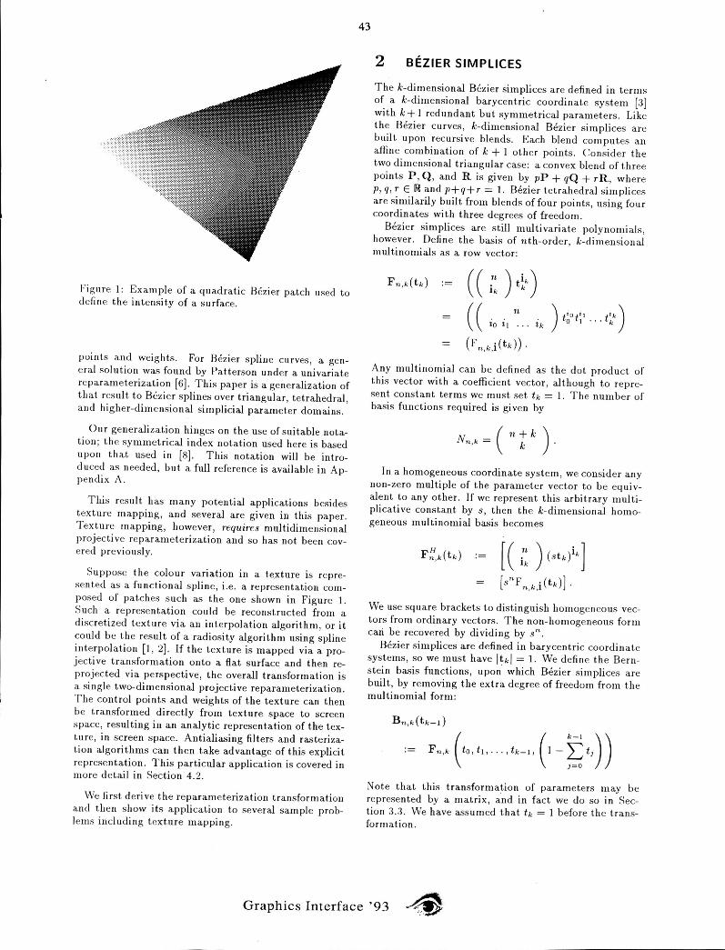
Figure 1: Example of a quadratic Bezier patch used to defin e the intensity of a surface.

points and weights . For Bezier spline curves, a gen­eral solu tion was found by Patterson under a univariate reparamete rization [6]. This paper is a generalization of that result to Bezier splines over triangular, tetrahed ral , and higher-dim ension al simpli cial parameter domains.

Our generalization hinges on the use of suitable nota­tion; th e symmetrical index notation used here is based upon that used in [8]. This notation will be intro­duced as needed, but a full reference is available in Ap­pendix A.

This resul t has m any potential applications besides texture mapping , and several are given in this paper. Texture mapping , however , requires multidimensional projecti ve reparameterization and so has not been cov­ered previously.

Suppose t he colour variation in a texture is repre­se nted as a functional spline, i.e. a representation com­posed of patches such as the one shown ·in Figure 1. Such a representation could be reconstructed from a discretized texture vi a an interpolation algorithm, or it co uld be th e result of a radiosity algorithm using spline interpolation [1 , 2]. If the texture is mapped via a pro­jecti ve transformation on to a flat surface and then re­projected via perspective, the overall transformation is a single two-dimensional projective reparameterization . The control points and weights of the tex ture can then be transformed direc tly from texture space to screen space, res ulting in an analytic representation of the tex­ture, in screen space. Antialiasing filters and rasteriza­tion algorithms can then take advantage of this explicit representation. This particular appli cation is covered in more detail in Section 4.2.

We first deri ve the reparameterization transformation and then show its application to several sample prob­lems including texture ma pping.

43

2 BEZIER SIMPlICES

The k-dimensional Bezier simplices a re defined in terms of a k-dimensional barycentric coordinate system [3] with k + 1 redundant but symmetrical paramete rs. Like the Bezier curves, k-dimensional Bh ier sim plices a re built upon rec ursive blends. Each blend computes an affine combination of k + ]. other points . Consider the two dim ensional triangular case: a co nvex blend of three points P , Q , and R is given by pP + qQ + rR, wh ere 1) , q, r E Rand p+q+r = 1. Bezier tetrah edral simplices are simil arily built from blends offour points , using four coordinates with three degrees of freedom .

Bezier simpli ces are still multivariate polynomials , however. Defin e the basis of nth-order, k-dim ensional multinomials as a row vector:

) tiOtit tlk) , 0 1 .. . k tk

Any mul tinomial can be defin ed as the dot prod uct of this vector with a coefficient vector , although to repre­sent constant terms we must set h = 1. The number of basis functions required is given by

( n + k ) Nn.k = k

In a homogeneous coordinate system, we consider any non-zero multiple of the parameter vector to be eq uiv­alent to any other. If we represent this arbitrary multi­plicative constant by s, then the k-dirn ensional homo­geneous multinomial basis beco mes

[ ( ;: ) (stk) i k]

[s" F n.d (tk)]'

We use square brackets to distinguish homogeneo us vec­tors from ordinary vec tors. The non-homogeneo us form cari be recovered by dividing by Sn'

Bezier simplices are defin ed in barycentri c coordinate systems, so we must have Itkl = 1. We defin e the Bern­stein basis functions , upon' which Bezier simpli ces are built, by removing the extra deg ree of freedom from the multinomial form:

B n.dtk-d

Fn.k (to,t1, ... ,tk-1, (1 -~tj)) Note that this transformation of parameters may be represented by a matrix, ~nd in fact we do so in Sec­tion 3.3. We have assumed that h = 1 befo re the trans­formation.

Graphics Interface '93

With these definitions , we can finally define the nth order, k-dimensional homogeneously parameterized Bernstein-Bezier basis functions as

The nth order, k-dimensional homogeneous Bezier simplices P;;,k are defined by

44

where pHis a N n,k X (m + 1) matrix; a column vector of row vectors, each row being a m-channel homogeneous control vertex of the form :

The superscript is a label , not an exponent. The switch value Pi is 1 for finite control points and 0 for points at infinity. The value wi is called the weight of control

vertex pf . The matrix of control vertices can be factored into

the product of a diagonal weight matrix Wand a nor­mali zed version of the control points QH:

pH WQH

diag( Wi) ([pi, pi, ... pi, Pi]) .

This defin es a Bezier simplex over the projective pa­rameter space RPk. Therefore, P ;; k is an injective map from Rpk into Rpm, where Rpl is the real projective space of dimension t.

The form of the nth order rational Bezier simplex, after normalization , is given by

which is a m-dimensional row vector indexed by q, the channel index. Because of the fact that the Bernstein basis forms a partition of unity, this reduces to a. non­rational form if all weights are equal and all control poin ts are fini te:

R

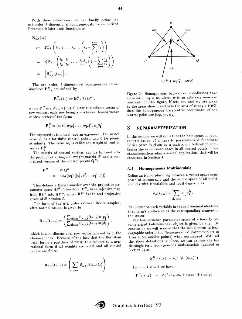
p Q

WpP + wqQ + wTR

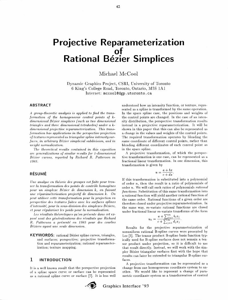
Figure 2: Homogeneous barycentric coordinates have wp + WT + wq = w, where w is an arbitrary non-zero constant . In this figure , if wp, WT, and wq are given by the areas shown, and W is the area of triangle P RQ, then the homogeneous barycentric coordinates of the central point are [wp, WT, wq] .

3 REPARAMETERIZATION

In this section we will show that the homogeneous repa­rameterization of a linearly parameterized functional Bezier patch is given by a matrix multiplication com­bining the same ·coordinat~s in all control points. This characterization admits several applications that will be examined in Section 4.

3.1 Homogeneous Multinomials

Define an isomorphism rPn between a vector space com­posed of tensors Sn,k and the vector space of all multi­nomials with k variables and total degree 11 as

rPn(Sn,k) = L: sik X~k.

li k I=n

The power on each variable in the multinomial identifi es that term's coefficient as the corresponding element of the tensor.

The homogeneous parameter space of a linearly pa­rameterized k-dimensional object is given by Sl,k. By convention we will assume that the last element in lexi­cographic order is the "homogeneous" parameter, set to 1 (or 0, for infinite points) when normalized . With all the above definitions in place, we can express the ba­sic single-term homogeneous multinomials (defined in Section 2) as

For 11 = 1, k = 2 we have

Graphics Interface '93

[

Foo l

F OIO

F IOO

8001 8010 SIOO r

and for It = 2, k = 2 we have

~ .:;' ( 860 1 X6 + 861OX ~ + s~oox~ + 28oolsoloxoxI + 28001 SI00XOX2

+ 2S0108100XIX2

Fo0 2 8501 FOil 2800 I So 10 F 020 8610 FIO I 2800 1 SIOO F l lo = 280108100 F 200 8ioo

3 .2 Projective Reparameterization

) T

A projective reparameterization of a k-dimensional ho­mogeneo us multinomial can be represented by a (k + 1) x (k + 1) matrix post multiplying the parameter vec­tor . For any given (k + 1) x (k + 1) matrix M = [mij], the repa rameterized multinomials are given by

ljJ;; 1 (ljJI (sl,kMr)

ljJ;; 1 (ljJI (SI ,kr) on ,k(M)

We can find the Nn,k x Nn,k matrix on,k(M) by direct sy mbolic computation I or by transforming the generat­ing fun ction into a combinatoric expression . See Ap­pendix C for specific examples, and Appendix B for the com binato ric form of this operator.

The combinatori c operator On ,k is a homomorphism of the group of (k+ 1) x (k+ 1) matrices; a proof is provided in Appendix B. Therefore in verses map to inverses, and m at rix mul tiplications inside the isomo rphism can be moved outside by mapping the component matrices through the On ,k operator.

3 .3 Reparameterization of Bezier Simplices

The On ,k (M) matrices only al low reparameterization of homogeneo us multinomials. To reparameterize Bezier simplices, we have to preceed the reparameterization matrix by a matrix that transforms the multinomials into Bezie r bas is functions. Such a matrix for triangles is given by

o -1 ) - 1 . 1 o

The inverse of this matrix , which we shall need later , is given by

I Maple cod e is avail able dgp .ut'o ro nto.ca (128 .100 .1.129) .

o 1 o

via a no nymous ftp from

45

We will also define Mn = On.k\Mt}; since On ,k is a ho­momorphism , M;;I = on ,k(M I- ). The generalization of these matrices to higher dimensions should be obvious. Now

F ;;'dsl,kMI )

F ;;,k(SI ,k )Mn .

Defin e ' the matrix operator pn,k such that

We have

F;;'dSI ,k )On ,k(A)Mn

F;;,k(SI,kA)Mn

B ;;,dsl ,kA)

B ;;,dsl ,k)Pn,d A )

F ;;,dsl ,k )MnPn ,k (A) .

Therefore, Pn,k is a conjugate representatiGil to On,k:

M;:IOn ,k(A)Mn

On ,k(M I-I AMI)

Recall our definition of a patch expressed as a matrix product:

P ;;,dSl ,k) = B ;;,dsl,k) pH

.

If we substitute our expression for an arbitrary proJec­tive reparameterization , we get

where

B ;;,dsl,kA) p H

B ;;'dsl,k )Pn ,k (A) p H

B ;;,dsl ,k)VH

,

is the new set of control points. This transformation can also be expressed as

v H = Pn ,i.(A)WQH

for normalized control points. If Pn ,k(A) is diagonal, then only the weights need to be changed to carry out the reparameterization.

3 .4 Complexity

A projective reparameterization of a Bezier simplex co r­responds to a projective transformation of each coo rdi­nate of its control points, treated together as a vector in Nn,k-dimensional space. The transformation of these control points is combinatorically related to the repa­rameterization matrix A, and is given by the Nn ,k x Nn ,k matrix pn k(A). Performing the matrix multiplication Pn ,dA) p H requires O((m + l)N~,d operations for m channels, with no assumptions about weights. It should be noted t hat Nn,k = O(nk) , so the complexity m ay be

G raphic s In terface '93

written 0(mn2k ). Compare this to a spatial projec­ti ve transformation gi ven by a (k + 1) x (k + 1) ma­trix B: VH = p H B. This multiplication requires only O((k + 1)2 Nn ,k) = 0(k2n k ) operations.

Summary: the upper bound on complexity of general reparameterization has an ex tra factor of O(m;t k /k2) over spat ial transformation . This res ult does not pre­clude special cases from being more effi cient , however. For some matri ces A , Pn,k(A) may be sparse, di agonal, or afford a recursi ve factorization into sparse ma trices.

4 APPLICATIONS

In this section we cover some specific applications of the relationship we have derived.

4. 1 Weight Normalization

I t is known in the case of rational Bezier curves that varying patterns of weights can lead to the same space curve, al bei t wi th different pa rameterizations . A curve is considered to have a normalized weight pattern when Wan = 1 and WnO = 1.

Correspondingly, we defin e the weight pattern of a surface to be normalized wh en the weights at all "cor­ilers" have been set to 1. Corners have one index se t to n and all others set to O. This normalization must be acco mplished without changing th e sha pe of the s urface, and prefera bly by only changing the weights.

Consider first th e problem of normalizing a su rface that uses the hom oge neous multinomials Ft: k as a basis. T he surface is given by ,

for some matri x of normalized homogeneo us control points Q H and matrix of weights W = diag(wi)' Define the reparamete rizi ng transformation matrix

Ark = diag(To, TI , ... , Tk).

This transformation fixes the corn er paramete r values in IRpk, since constant factors can be ignored in proj ective space.

TO (1,0,0, ... , 0) (l,O,O, ... ,O)Ark TI(0 , 1,0, ... , 0) (0,1,0, ... , 0)Ark T2(0 , 0, 1, ... , 0) (0 , 0, 1, .. . ,0)Ark

Tk(O, 0, 0 ... , 1) (0,0 , 0, ... , 1 )Ark •

If the parametric co rn er points are fixed in projective space, th en the shape of the resulting curve will be un­changed.

Consider on ,k( A r k ). Each entry in this matrix is com­posed of sums of products of entries of Ark' Only diag­onal elements contain terms t hat are composed entirely of diagonal elements of A. TherefC:re, if Ark is diago­nal then so is on,dAr k ) and on,dA~k)W , The weights

46

will chan ge but the Euclidean positions of the co ntrol verti ces will not .

Create the vector Vn ,k to contain the di ago nal entri es of b",dA"k)' It can be seen that the ith element of v

will be equal to ri . Therefore, to normali ze the corn er weights , we simply set the elements of rk as foll ows:

TO WOOO .. 00n

Wooo . . 0nO

Tk_1 WO nO .. 000

WnOO .. 000

Furthermore, let.

Brk MIAr.M~1

TO 0 0 0 TO - Tk 0 TI 0 0 TI - Tk 0 0 T2 0 T2 - Tk

0 0 0 Tk-I Tk-I - Tk 0 0 0 0 Tk

This reparameterization fixes the projective parameters

TO (1 , 0 , 0, ... , 0 , 1) (l , O, O, . .. , O, l )Brk

TI (0 , 1, 0, ... ,0, 1) (0,1 , 0, ... , 0, 1)Br.

T2 (0, 0 , 1, .. . , 0, 1) (O,O , l , ... , O, l)Br k

rk(O , O, O, ... ,O, l) (O,O,O, ... , O,l)Br • .

Sin ce the' paramet ri c corners of the Bezier patch are fixed , the shape will remain unchanged .

Note that Pn,k(Brk ) on , k(M~1 Br.MI ) bn,k (Ar.) , so we can state the Bezier reparameteriza­tion using Brk :

pH (SI ,k Br.)

pH (SI ,k)

B t:,dsl ,k Brk)WQH

Bt:,k (SI ,k)Pn,k{ Br. )WQ H

Bt:,k (SI ,k)On ,k (Ark )WQ H

B t:,dsl,k)W'QH.

The matrix Brk gives the same transformation as Ark ' but with respec t to the Bernst ein-Bezier basis .

4. 2 Perspective Reparameterization

Perspective projection is the most obvious a nd in­escapable non-affine projective transformation in com­puter graphics. The persp ective projec tion of a flat t ex­t ure mapped polygon results in a projective reparame­teri zation of the colour function. Hence, if the texture is

Graphics Interface '93

represented as a two-dimensional fun ctio nal Bezier sur­face , then the rational Bhier representation in screen coo rdinates may be found .

We first review the parameterization , projection, and transformation composition process that takes place during texture mapping.

4.2.1 Texture Transformations

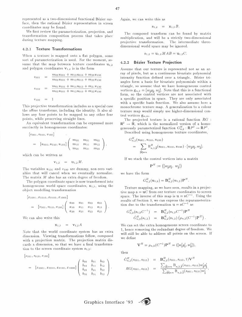
When a texture is mapped onto a flat polygon , some sort of parameterization is used. For the moment , as­s um e that th e map betwee n texture coordinates UI ,2 and polygon coordinates VI ,2 is in the form

rnOOUOOI + rnlOUOIO + m 20 UI OO VOOI + rnl2UOIO + 1n22UIOO 17L02UOOI

rnOI UOOI + 1nl I UOIO + 1n21 UIOO VOIO

rn02UOO I + 1n12UOIO + 1n22UIOO

This projective transformation includes as a special case the affine transforms, including the j.dentity. It also al­lows any four points to be mapped to any other four points, while preserving st raight lines .

An equivalent transformation can be expressed more succinctly in homogeneo us coo rdinates:

[VOOI, VOIO, VIOO ]

( rn oo rn OI l1L0 2 ), [UOOI, UOIO, UIOO] rnl O rnll rnl 2

rn20 7n21 rn22

which can be written as

VI ,2 UI ,2M.

The variables UIOO and VIOO are dummy, non-zero vari­a bles that will cancel wh en we event ually normalize. The matrix M also has an extra degree of freedom .

The polygon coordinate space is now transformed into h O lllogeneo ~ s world space coo rdinates, XI ,3, using the object modelling transformation

[ XOOOI , XOOIO , XO I OO, XIOOO]

[ VOO I ,VOIO,V I OO ] (

aOO aOI a02 a03 ). alO all al2 al 3

a20 a21 a22 a23

We can also wri te this

XI ,3 VI ,2A

Note that the world coordinate system has an extra dimension . Vi ewing transformations follow , composed with a projection matrix. The projection matrix dis­cards a dim ension , so that we have a final transform a­tion to the screen coordinate system SI,2:

[SOOI, SOlO, SIOO ]

[,,'"' , ,,",,, "'"', ","00] ( )

47

Again, we can write this as

SI,2 XI ,3 B .

T he composed transform can be found by matrix multiplication, and will be a strictly two-dimensional projec tive transformation. The intermediate three­dimensional world space may be ignored.

4.2.2 Bezier Texture Projection

Assume that our texture is represented not as an ar­ray of pixels , but as a continuous bivariate polynomial intensity function defin ed over a triangle. Bezier tri­angles form a basis for bivariate polynomials within a triangl e, so assum e that we have homogeneo us control verti~es gn ,2 = [wigi , wi]' Note that this is a functional form , so the co ntrol vertices are not associated with a specific position in space. They are only associated with a specific basis function . We also assume here a monochrome texture map. A generalization to a colour texture map would simply use higher-dimensional con­trol vertices g n,m.

The projected texture is a rational fun ction RC : !R2

-+ !R , which is the normalized version of a homo­geneously parameterized fu.nction C;;,2 : !Rp2 -+ !Rpl .

Desc ribed using homogeneous texture coo rdinates,

C;;'2(UOOI, UOIO, UIOO)

L B:,I,i(uOOI ,UO IO,UIOO)' [w igi ,wi]'

lil=n

If we stack the control vertices into a mat rix

we have the form

C;;,2(UI ,2) = B;;,2(UI ,2) pH .

Texture mapping , as we have seen, results in a projec­tive map S = uC from our texture coordinates to screen space. The inverse of this map is U = sC- I. Using the res ults of Section 3, we can express the reparameteriza­tion due to th e transformation u = sC- 1 as

C;;,2(SI,2C- I )

(;;;'2 (SI,2)

We can set the extra homogeneous screen coordinate to 1, hence removing th e redundant degree of freedom. We will still be able to address all points on the screen. If we defin e

H -I) H ([" ']) Y = Pn ,k(C P = wigi, wi '

then

B;;:2(SOOI,SOI0, 1)yH

RC( SOOI , SOlO) Llil=n Bn ,2,i (SOOI, SOlO )wigi

Llil=n Bn ,2,i (SOOI, sOIO)wi '

Graphics Interface '93

4.2.3 Evaluation

To evaluate the texture map in screen space, we need to evaluate RG( SOO I , SOlO) which is a ratio of linear CO Ill ­

binations of Bezier bas is functions in screen space.. U n­fortunately, every new output control value depends, in ge neral , on every input control value. This non-locality limits the practical use of this technique, unless the tex­ture is broken up into many segments of low order. For cubic triangles , N 3 ,2 = 10, and so a brute-force transfor­mation of a single segment requires 200 multiplications and 180 additions, not to mention the computation of Pn ,k «(,'-1). Since N2 ,2 = 6, quadratic triangles require 72 multiplications and 60 additions. Linear tri angles require 18 multiplications and 12 additions. .

In the special ca'5e in which all the control points have been normalized so all wi = 1, then half the multipli­cations may be eliminated. This is the case where the source is always known to be a polynomial , which can be a rranged in a texture mapping application .

4.3 Arbitrary Subdivision

Suppose we were given a triangular rational Bezier patch and needed to extract som~ arbitrary triangular subpatch, with the subpatch represented a'5 a triangular Bezier patch (i. e. in terms of control points).

Defin e the parametri c corners of the su bpatch by the homogeneous parameters

a ( aOO 1 , ao 10 , a 100 ) ,

b (bool , bolo , blOo ) ,

c (C001 , C010,C 100).

To create the subpatch, we have to describe a transfor­mation t hat maps

aM Sa = (1,0,0),

bM -+ Sb = (0 , 1,0),

cM S e = (0,0 , 1) .

Such a transformation is given by

a0 10

bolO

C0 10

alOO ) blOo M l .

C100

We define this matrix by its inverse because the inverse is exactly what will be needed .

Recall that a rational, triangular Bezier patch is given in homogeneo us coordinates by .

We can reparameterize this patch so that the desired triangle lies in the stand ard parameter range using th e param eter transformation Ul ,2 = Vl ,2 M- l :

P ;;,2(Vl ,2M- l)

i> ;;,2 (Vl ,2 )

B;;,2 (Vl,2 M-I )pH ,

B;;'2(Vl ,2 ) (Pn,2(M -l )p H),

B;;'2(Vl ,2)yH.

48

The control points of the subdivided patch are th ere­fore yH = Pn,2(M- l )pH . Once again , this is a rel­atively expensive operation; however, the fact that it is totally general can be useful in some cases. There are, for example , no restrictions on the orientation of the subpatch with respec t to the larger patch, and no special ca'5es.

5 CONCLUSIONS

A multidimensional generalization of a 1-D result has been presented . The general theoretical result ha'5 many applications, although specialization is needed to derive effici ent algorithms. Application of the techniques pre­sented in this paper results in algorithms for a variety of applications of rational reparameterization of poly­nomial spline surfaces, including weight normalization , texture mapping , and subdivision.

6 ACKNOWLEDGEMENTS

The long-term financial support of the Natural Sciences and Engineering Research Council of Canada and the lnformation Technology Research Centre of Ontario is gratefull y acknowledged . Our graphics lab has also ben­efi ted from the generous financial support of Alia'5 Re­search, Apple Computer, DEC and Xerox Corp.

The referees provided useful suggestions that led to an improvement in the notation from horrific to merely baroque; the readers should be as thankful as the author is! Eugene Fiume provided additional assistance in this regard.

Timely and appreciated assistance in the translation of the abstract into a r esume fran~ais was provided by Michiel van de Panne, Kim H. Veltman , and Marc Ouel­lette.

A NOTATION

The objects used to construct Bezier simplices are most properly understood as tensors. A symmetrical multiin­dex notation is used to refer to elements of these tensors and they are implicitly stacked in lexicographical ord er: This is formalized in the foll owing sections.

A.I Tensors and Multiindices

Defin e the simplicial tenso r Sn ,k := {si.} such that h =

{io, il , . .. ,id with ij EN and Ihl:= L~=oiJ = 11. Note that the multiindex h has k+ 1 elements , although it is redundant and should be considered as only having dimension k. .

We will call k the order of the tensor Sn ,k , and 11 th e dimension. The short form Sk := Sl ,k may be used for one-dimensional vectors, hence i k = il ,k. When pos­sible and unambiguo us, we will leave out comma') in su bscripts of the elements of tenso rs.

Graphics Interface '93

Examples:

81 ,2 (SOOI,SOIO , SIOO)

~ {soo~l,o~~,olO} 82 ,2 ( S 002 , SOII,S020,SI01 , 8110,S200)

~ { SIO~~O~;IO ' }

S002, SIOI, S020

For a one-dimensional tensor Xk , define exponentia­tion by a multiindex of the same dimension as

Define the multiindex combination , with lik I = n , as

( n ) h

n

nk 'I j=O l).

n

A. 2 Stacking

Tensors are somewhat awkward to work with, especially tensors of the form used here, where the entire multiin­dex has to be considered to determine a valid (or equi v­alently, non-zero) element of the tensor. While keeping the tensor structure in mind, we would like to map the variables into a familiar matrix-vector form. This we can accomplish with a stacking operator. The stacking operator simply arranges the elements of a tensor in a specific order wi thin a row vector. A matrix can then specify arbitrary linear combinations of tensor elements to create a new tensor.

The stacking operator is defined by any bijective map­ping On,k : N k + 1 -+ N of the multiindex onto a single index: i = On,k(h). This mapping is invertible by defi­nition.

There are many possible stacking maps, but to make the mathematics cleaner we can choose maps that sat­isfy some simple conditions. The stacking map should map (0,0, .... , n) to 1, should not have any gaps, and should be lexicographically ordered.

A mapping that satisfies these conditions in two di­mensIOns IS

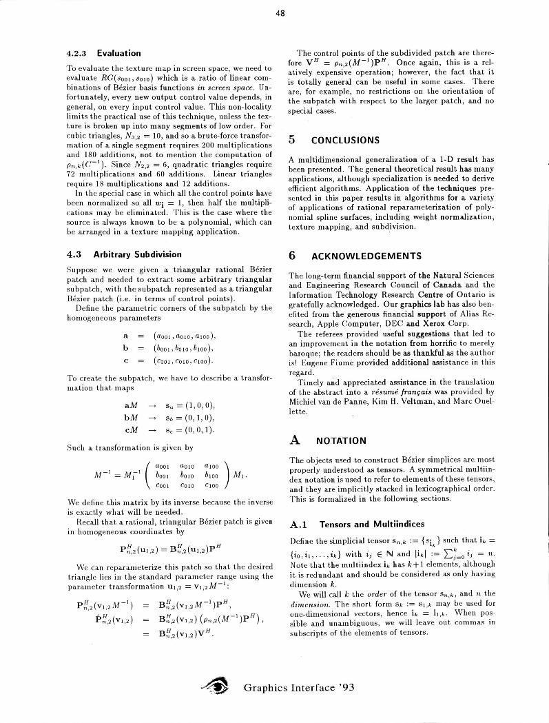
An example for 11 = 5 is given in Table 1. The maximum value in this mapping, which is also

the number of tensor elements, is given by

. (n+l)(n+2) N n ,2 := On,2(12 = , nOO) = 2 .

Note that we typically write multiindices in reverse order in subscripts , so that the most significant digit

49

5 16 Os ,2(i2, i l , io) 4 11 17 3 7 12 18 2 4 8 13 19

1 1 2 5 9 14 20 II 0 1 3 6 10 15 21

0 1 2 3 4 5 l2 ---+

Table 1: Example mapping between tensor and linear indices for n=5,k=2 (three-variable multiindices). Note that io is redundant.

comes first. In other words, the index 102 indicates io = 2, i l = 0, i2 = 1.

In general, these mappings are generated by [4] (pp. 297- 298,303):

O (')'_2:k (k-.r-1+Lik=+lii) n k Ik ._ T. , k-r r=O

For example, the mapping 1Il three dimensions would be

On,3(h) =

=

( 2 + i3 i i2 + i 1 )

+ ( 1 + i~ + i2 ) + ( i; ) + 1

(2 + i3 + i2 + iI)(l + i3 + i2 + iI)( i3 + i2 + i1) 6

(1 + i3 + i2)( i3 + i2) , + 2 + '3 + 1.

Inverses of these maps may be computed via a lookup table.

B PROOF OF HOMO MO RPHISM

If M is a (k+ 1) x (k+ 1) invertible matrix , let 4>n(M) be the column vector of multinomials obtained by applying </>n to every row of M . Let 4>n(M) = (pj(Xk))T = Pk(Xk)T, where pj(Xk) is a multinomial in Xk and j is the index of the corresponding row in M.

Before continuing with the proof of homomorphism, we need the following:

LEMMA: Given Vk E Rk +1 and M an invertible (k + 1) x (k + 1) matrix, tlien </>n(vkM) = vk4>n(M).

PROOF OF LEMMA: Let an,k = (xikf be an Nn,k el­ement column vector containing the power basis of multinomials in Xk of total degree n. Then </>n(Vk) = Vkan,k, and

(vkM)an,k = vk(Man ,k) vk4>n(M) . •

Graphics Interface '93

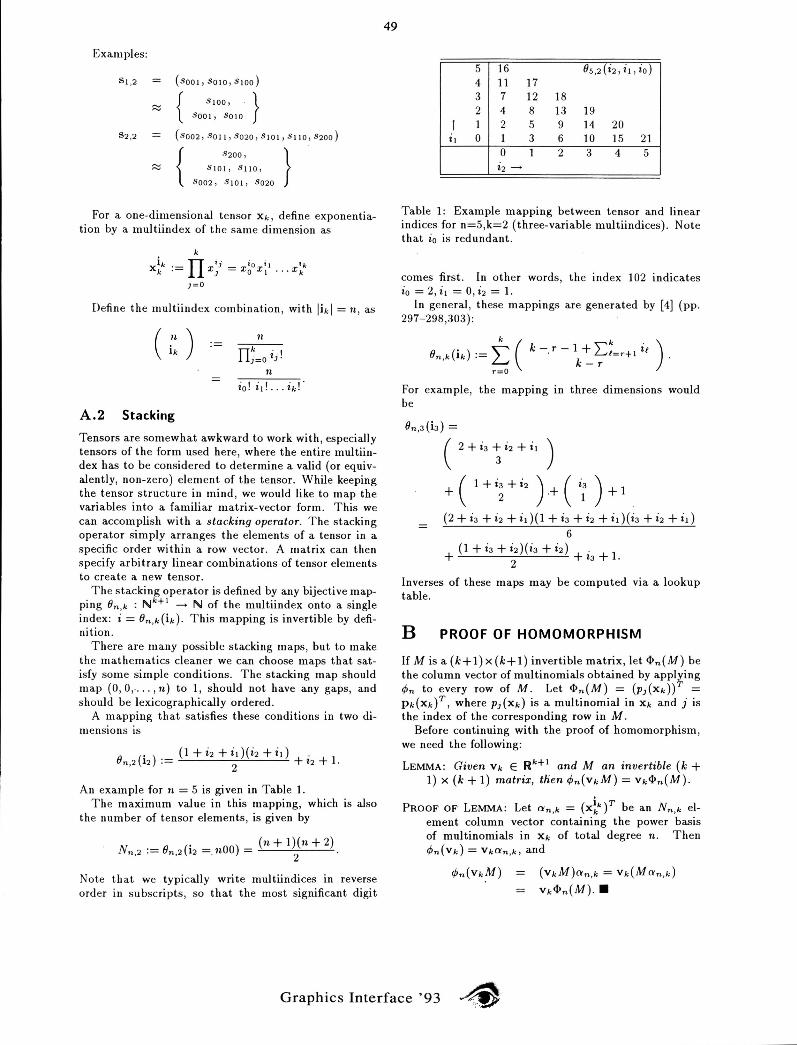
Now we can prove the following theorem, which shows that the reparameterization can be externalized , and also gi ves a more explici t form for eval uating the com­bina torical matrix:

THEOREM 1: If Dn ,k (M) is defin ed by

Fn ,k(SkM) = Fn ,dSk)Dn ,d M ),

th en

Dn ,dM) = pg(Xk)p?(Xk) ... pL, (Xk)Pk(Xk) pg(Xk)P?(Xk) .. . pi-, (Xk)pZ-' (Xk) pg(Xk)P?(Xk) ... pi-, (Xk)pZ-2(Xk)

l)g-' (x k)pl (Xk) . . . pL , (xkh)~(Xk) PO'(Xk)P?(Xk) .. ·pL, (Xk)p~(Xk)

= ~~' ( (pik (Xk)) T) .

PROOF OF THEOREM 1: Combine the Lemma and the multinomial theorem:

,p;; ' (,p ,(skM),,)

,p ;;' ({sk~,(M)}n)

.~ ' ( {t. ,,p,(x,) n ,p ;;' (.2: ( ;: ) S~kP~k(Xk))

Il k I=n

50

,p;; ' (( ( ;: ) S~k) (p~k (Xk) f)

( ( ;: ) S~k ) ~;;' ( (p~k (Xk)f) Fn ,k(Sk)Dn ,k(M) . •

THEOREM 2: The operator Dn ,k is a homomorphism of th e gmup of invertible (k + 1) x (k + 1) matricies.

PROOF OF THEOREM 2: Let A , B be two invertible (k+ 1) x (k + 1) matrici es. Note that

Fn ,k(Sk(AB))

Fn ,k((SkA)B)

Fn ,k(Sk )Dn,k(A B) ,

Fn ,k (Sk )Dn ,k(A )Dn ,k (B) .

By the associativity of matrix multiplication, we must have D" ,k(AB) = Dn,k(A)Dn,d B) on th e linear span of Fn ,dsk). Since Fn,dsk) spans all of Rk+', D,. ,k is a homomorphism. •

C COMBINATORIAL MATRICES

Let

M= ( ~ G

b e H

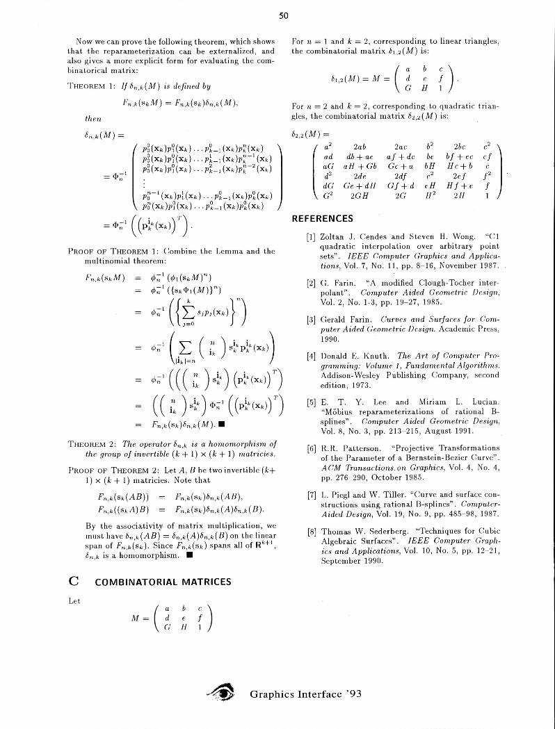
For n = 1 and k = 2, co rres ponding to linear triangles, the combinatorial matrix D, ,2 (M) is :

D,,2(M) = M = ( ~ b { ). e

G H

For n = 2 and k = 2, co rresponding to quadra ti c tri an-gles, the combinato ri al matrix D2,2(M) is:

D2 ,2 (M) =

( a' 2ab 2ac b2 2bc c2

) ad db+ ae af + dc be bf + ec cf aG aH + Gb Gc+a bH Hc +b c d2 2de 2df e2 2ef f 2

dG Ge+dH Gf+d eH Hf+ e f (;2 2G H 2G H2 2H

REFERENCES

[1] Zoltan J. Cendes and Steven H. Wong. "C l quadratic interpolati on over a rbitrary poin t sets". IEEE Computer Graphics and Applica­tions , Vo!. 7, No. 11 , pp . 8-16 , November 1987.

[2] G . Farin. "A modified Clough-Tocher inte r­polant". Computer Aided Geometric Design, Vo!. 2, No. 1-3, pp. 19- 27, 1985.

[3] Gerald Farin. Curves and Surf aces f or Co m­puter A ided Geometric Des ign. Academic Press, 1990.

[4] Donald E. Knuth. Th e A7·t of Computer Pro­gramming: Volum e J, Fundam ental Algorithms. Addison- Wesley Publishing Company, second edition , 1973.

[5] E.T. Y. Lee and Miriam L. Lucian. "Miibius reparameterizations of rat ional B­splines" . Computer A ided Geometric Desigll, Vo!. 8, No. 3, pp . 213- 215 , August 1991.

[6] R. R. Patterson. " Project i ve Transformations of the Parameter of a Berns tein-Bezier Cu rve" . ACM Transactions . on Graphics, Vo!. 4, No. 4, pp. 276-290 , October 1985.

[7] L. Piegl and W . Tiller. "Curve and surface co n­structions using rational B-splines". Computer­Aided Design, Vo!. 19 , No. 9, pp. 48.')-98, 1987.

[8] Thomas W. Sederberg. "Techniques for Cubic Algebraic Surfaces". I EEE Computer Graph­ics and Applications, Vo!. 10 , No. 5, pp . 12- 21, September 1990.

Graphics Interface '93