Propagation of Financial Shocks in an Input-Output Economy

with Trade and Financial Linkages of Firms

Job Market Paper

updates at: http://www.columbia.edu/~sl3256/research.html

Shaowen Luo∗

Columbia University

December 2, 2015

Abstract

Firms are connected through the production network. At the same time, the pro-

duction linkages coincide with financial linkages because of delays to input payments.

This paper investigates how these interconnected production and financial linkages lead

to the propagation of financial shocks both upstream and downstream. First, I show

that financial shocks can propagate upstream if there are financial linkages of firms

and financial frictions in trade. Second, I find, based on the input-output matrix and

the bond yield data in the U.S., upstream propagation of financial shocks is stronger

than downstream propagation. Third, I elaborate a DSGE model that can capture this

pattern of shocks and generate quantitative predictions. Fourth, I demonstrate that

credit policies would have a stronger impact if liquidity were transferred to downstream

sectors after aggregate liquidity shocks.

1 Introduction

An economy is an entangled network of specialized productions that are interconnected

through inter-firm trade within and across sectors. In the course of this trade, the products

∗Department of Economics, Columbia University, 420 W 118 St, New York, NY 10027(sl3256@columbia.edu). I am grateful to Ricardo Reis for his constant guidance and support. I would alsolike to thank Jushan Bai, Richard Clarida, Gauti Eggertsson, Jennifer La’O, Frederic Mishkin, Emi Naka-mura, Serena Ng, Stephanie Schmitt-Grohe, Jon Steinsson, Alireza Tahbaz-Salehi, Martin Uribe, MichaelWoodford, Pierre Yared for their invaluable advice. Discussions with and comments by Sergey Kolbin, Sav-itar Sundaresan, Daniel Villar and other seminar participants at Columbia greatly improved this paper. Allremaining errors are mine.

1

of one firm may be purchased and consumed by another firm as inputs. In addition, there is

often a waiting period between the moment in which a cost is incurred and the later point at

which cash flow materializes. In this way, the production network also creates and sustains

a trade credit network. An idiosyncratic financial shock may therefore spread through the

production and financial linkages of firms. It is necessary to determine how the interaction

between the production network and the trade credit network affects the propagation of

financial shocks.

The automotive industry crisis of 2008-2010 offers an example of how a financial shock to

one firm impacts its suppliers and customers. First, a financial shock to a firm may reduce

its demand for the goods and services of its suppliers. For example, General Motors Co.

significantly reduced its demand owing to a severe liquidity problem.1 Consequently, Amer-

ican Axle & Manufacturing Holdings Inc., one of the major suppliers of GM, experienced a

net loss of $112.1 million in the fourth quarter of 2008.2,3 Second, when a firm experiences a

financial shock, it may postpone repaying trade credit to its suppliers and reduce the provi-

sion of trade credit to its customers.4 For example, General Motors Co. and Chrysler Group

LLC. had in excess of $21 billion in domestic trade payables as of September 30, 2008.5 The

failure to meet these payments soon crippled GM’s suppliers during the crisis.

This paper builds an input-output model with trade credit to facilitate the study of the

propagation of financial shocks. To begin with, a simple network model is presented in

an effort to explain the mechanism behind the propagation of financial shocks, specifically

a static model with a vertical production network structure and financial linkages among

firms. To capture financial frictions, I assume that firms have a working capital requirement

on inputs, and thus need to pay wages and intermediate input costs in advance of production.

To satisfy this requirement, firms acquire loans as well as trade credit from suppliers. Ac-

cordingly, firms are financially interlocked through trade: suppliers can use payments from

customers as working capital, while at the same time the balance sheets of trading parties

become interlocked through accounts-payable and accounts-receivable.

My model shows that the production and financial linkages among firms serve to prop-

agate financial shocks both upstream and downstream. A positive borrowing cost shock to

1A combination of tight credit and declining sales caused the crisis in the U.S. auto industry from 2008to 2010. This paper focuses on the impact of credit contraction in the production network.

2“American Axle CEO: ‘2008 Is the Year From Hell’.” 30 January 2009, Dow Jones International News.3Similarly, in the 1997 Korean financial crisis, Kia Motors suffered liquidity problems that affected its

16,000 domestic suppliers. Source: “South Korea’s Kia Buckles, And Suppliers Begin to Break.” 22 August1997, The Wall Street Journal .

4Trade credit is the single most important source of external finance for firms (Boissay and Gropp (2007)).Trade credits are short-term loans that a supplier provides to a customer upon purchase of its product, andthat thus constitute a form of deferred payment. A discussion of trade credit is provided in Appendix A.

5“US CREDIT - A GM failure risks more debt losses, default chain.” 11 December 2008, Reuters News.

2

loans increases the input cost, reduces intermediate input demand and affects intermediate

input suppliers. This is upstream propagation. The same shock increases the production

price, which creates supply impact and affects product consumers. This is downstream

propagation. The mechanisms behind these processes are as follows.

Two countervailing effects determine the extent of upstream propagation following a

positive borrowing cost shock: the income effect decreases intermediate input demand, since

production falls on account of the financial distress; the substitution effect, on the other hand,

increases intermediate input demand. Because of delays to intermediate input payments,

the marginal cost of intermediate input is less sensitive to borrowing cost shocks than is the

marginal cost of labor. Consequently, firms will substitute labor with intermediate inputs

after the shock. An important aspect of trade credit is that it amplifies the substitution

effect and attenuates upstream propagation of a shock.

In like manner, two countervailing effects determine the extent of downstream propaga-

tion following a shock: the cost effect increases product price, while the discount effect de-

creases product price. Products are sold to downstream firms, which make early payments,

and to households, which make late payments. Because producers value early payments,

there is a price discount for downstream firms. Here again, trade credit plays a significant

role, this time by weakening the discount effect and amplifying downstream propagation.

The relative strength of upstream versus downstream propagation therefore depends on the

level of trade credit.

Next I examine whether upstream or downstream propagation of financial shocks is re-

vealed in the data, which in my analysis suggests that upstream propagation of financial

shocks is stronger than downstream propagation. Using changes in sectoral bond yields as

an indicator of idiosyncratic financial shocks to each sector, I find that sectors are more sen-

sitive to financial shocks that hit their customers than to shocks that hit their suppliers. A

1% change in the bond yield of the customers of a sector generates a negative 0.17% output

change in the focal sector. The same shock hit the sector’s suppliers, by contrast, has no

significant impact on the focal sector.

Afterwards, I use a DSGE model to numerically examine the transmission of idiosyncratic

financial shocks. The input-output structure is standard (and follows that of Long and

Plosser (1983) or Acemoglu et al. (2012)). In the economy, firms issue claims in order to

purchase capital and acquire loans in order to satisfy their working capital requirements.

Financial intermediaries supply liquidity to firms and face balance sheet constraints that are

endogenously determined, in keeping with the framework developed by Gertler and Karadi

(2011). Moreover, firms share liquidity with other firms through trade credit, just as in my

static model, while they retain some flexibility for adjusting the level of trade credit.

3

By analyzing the model, I find the following results. This model indicates that the up-

stream propagation of financial shocks is stronger than the downstream propagation. It also

demonstrates that trade credit increases the output correlation of firms. Furthermore, com-

pared with a representative firm model, aggregate variables in the network model are more

responsive to shocks of all kinds. The input-output structure generates a strong amplification

effect on the aggregate impact of shocks.

Finally, the policy implication of my model is that credit policies would have a stronger

impact if liquidity were transferred to downstream sectors after aggregate liquidity shocks.

According to Gertler and Karadi (2011), the severity of a recession could be mitigated if

policymakers were to supply liquidity during extreme economic conditions.6 Such was the

thinking behind the policy whereby Federal Reserve loans to private entities and other central

banks reached $1.5 trillion by the end of 2008 in the wake of the Lehman Brothers bankruptcy

(Price (2012)). However, which types of sectors or institutions should policymakers supply

liquidity to? The implications of credit policies that channel liquidity to specific sectors

or firms cannot be well studied by means of a representative firm model, though they can

be investigated using my model.7 My findings here suggest that it would be optimal if

policymakers target liquidity in downstream sectors following an aggregate liquidity shock,8

since the financial condition of downstream sectors is more important systemically, given

that financial shocks mainly propagate upstream. For example, credit policies that supply

liquidity to the construction sector would have stronger impacts than those to the utility

sector after a uniform liquidity contraction across sectors.

Literature review. To my knowledge, this is the first paper that studies the input-output

structure and trade-credit network in a general equilibrium framework. This project fits

into three strands of literature, namely (1) production networks; (2) trade credit; and (3)

financial frictions. Long and Plosser (1983) inaugurated the study of sectoral co-movements

6There are well-documented instances when just this policy was implemented. Thus, for example, theFederal Reserve granted the Continental Illinois National Bank and Trust Company access to the discountwindow from May 1984 through February 1985 despite the company’s effective insolvency, and in an earlierinstance, in 1970, it indirectly channeled credit to the commercial papers market in order to relieve thefinancial stress on the Penn Central Transportation Co. (Price (2012)). The bailout of General Motors Co. in2009 undoubtedly saved that firm’s suppliers from bankruptcy. Nonetheless, during the 1997 Korean financialcrisis, Kia’s suppliers complained that the liquidity injected into the banking system by Korea’s central bankhad failed to reach them. Source: “Auto Suppliers Turn Around: New Credit, Quick Restructurings of GMand Chrysler Sustained Parts Makers.” 26 December 2009, The Wall Street Journal. “South Korea’s KiaBuckles, And Suppliers Begin to Break.” 22 August, 1997, The Wall Street Journal .

7Using a heterogeneous agent model, Reis (2009) suggests that providing credit to traders in securitiesmarkets can restore liquidity with fewer government funds than extending credit to the originators of loans.

8Naturally, political barriers could complicate supplying liquidity to specific firms or sectors, though thefact is that policymakers do provide liquidity in this way during extreme economic conditions (such as theexamples provided in footnotes 5 and 6).

4

using a network model, sowing the seeds of a rich literature that has focused on the aggregate

volatility generated by idiosyncratic shocks.9 As presented by di Giovanni et al. (2014), there

are two effects that are at work. First, idiosyncratic shocks have sizeable aggregate effects

if there are strong input-output linkages between firms, which is the linkages effect (Bak

et al. (1993), Horvath (1998, 2000), Dupor (1999), Shea (2002), Conley and Dupor (2003),

Foerster et al. (2011), Acemoglu et al. (2012, 2015b), Jones (2011, 2012) etc.). Second,

idiosyncratic shocks can directly contribute to aggregate fluctuations, which is the direct

effect (Jovanovic (1987), Gabaix (2011), Carvalho and Gabaix (2013)). Of particular note

here is the study by Acemoglu et al. (2015a) of the propagation of supply and demand shocks

through input-output and geographic networks. My predictions for the propagation of these

types of shocks are consistent with their work. My emphasis, however, is on the transmission

of financial shocks in the input-output structure.

In research on the production network, financial frictions were not considered until the

study by Bigio and La’O (2013), following which Su (2014) and this paper represent contri-

butions to network-based approaches to the amplification of financial shocks. Aside from the

questions these three papers focus on, the nature of the financial friction in these three papers

is also different. Unlike Bigio and La’O (2013), my approach takes into account financial

linkages of firms and establishes a micro foundation for the financial sector. And while Su

(2014) presents a network model that accommodates financial frictions in the capital input,

he does not account for financial frictions in trade, for which reason his model is allocation-

ally equivalent to a horizontal one and can only describe the downstream propagation of

financial shocks.

Second, several theories have been put forward to explain why suppliers provide trade

credit to customers (e.g. Peterson and Rajan (1997), Burkart and Ellingsen (2004), Cunat

(2007)). My analysis follows that of Kiyotaki and Moore (1997) in emphasizing the role of

trade credit in the propagation of shocks. Regarding the third strand of inquiry, financial

frictions have been extensively studied in the literature on the 2008 financial crisis (e.g.

Gertler and Karadi (2011), Curdia and Woodford (2011)). This paper builds on these previ-

ous approaches in order to elaborate a heterogeneous firm model for the study of the impact

of idiosyncratic and aggregate financial shocks.

In what follows, Section 2 presents a simple static model to illustrate the propagation of

shocks in a chain economy. In Section 3, I discuss my empirical findings on the propagation

of financial shocks. Section 4 presents my DSGE model, and Section 5 calibrates the model

9There is also a branch of literature on the propagation of shocks in financial networks, e.g. Allen andGale (2000), Acemoglu et al. (2015c). The focus of this paper is the propagation of shocks in productionnetworks.

5

and forms quantitative predictions. Credit policy implications are the subject of Section

6. Section 7 concludes the paper with a summary of my findings and a discussion of their

implications.

2 A Simple Model

In this section I consider a simple economy in order to study the mechanism of the propa-

gation of financial shocks. In my model here, firms are connected vertically in a production

chain. The interconnected production and financial linkages among the firms lead to the

propagation of financial shocks both upstream and downstream.

Figure 1: Horizontal VS Network Economy

Firm 1 Firm 2 Firm 3

Final Output

a. Horizontal Economy b. Network Economy

Firm 1

Firm 2

Firm 3

Final Output

2.1 A horizontal economy with financial frictions

Before proceeding with this discussion, it will be useful to consider a horizontal economy

as the benchmark. In this simple economy, three firms produce three types of specialized

intermediate products m1,m2,m3 with prices p1, p2, p3 correspondingly. The flow of

goods in this economy is illustrated in Figure 1 panel a. Under these circumstances, there

are no connections among the firms, and labor li is the sole input of Firm i. Intermediate

sectors thus have the following production functions,

m1 = z1lα11 , m2 = z2l

α22 , m3 = z3l

α33 ,

where zi denotes technology. To capture financial frictions, I assume a working capital

requirement on labor exits. Firms in this case need to borrow in order to pay for their labor

6

cost at the beginning of each production period. I further assume a small open economy in

which firms obtain credit from the rest of the world with a fixed interest rate R. Policymakers

in addition impose a borrowing tax ei on each unit of the credit obtained by firm i.10 Thus,

the borrowing fee of firm i is Ri = R + ei. For simplicity, I assume that R = 1. The

tax revenue, which equals to the total borrowing cost, is distributed to households through

lump-sum transfers.

In this economy, the final output is

Y = Ξmζh11 m

ζh22 m

ζh33 , (1)

where Ξ is a constant, ζhi denotes the final share of product i. A representative household

solves the following problem,

maxC,L

log(C)− L, (2)

s.t. C = wL+ Ψ,

where Ψ represents the tax revenue distributed to households, and w is the wage rate.

Households make choices of consumption C and labor supply L subject to their budget

constraint. The market clearing condition of goods follows Y = C. The labor market

clearing condition follows L =∑3

i=1 li.

Given zi, Ri for i ∈ 1, 2, 3, a competitive equilibrium in this horizontal economy is

represented by a group of endogenous variables mi, li, L, Y , C, Ψ, pi, w for i ∈ 1, 2, 3,such that (1) each firm maximizes its own profits, (2) each household maximizes its own

utility, and (3) goods and labor markets clear.

The equilibrium results are presented in Appendix B.1.

2.2 A network economy with financial frictions

Unlike in a horizontal economy, firms in a network are interconnected through trade. Thus,

consider a production network in which three firms are vertically linked. The input-output

structure is illustrated in Figure 1 panel b. For the sake of simplicity, Firm 1 is the furthest

upstream, while Firm 3 is the furthest downstream. All three firms supply input that

figures in the production of the final goods. Each firm produces output using Cobb-Douglas

10The borrowing tax comes through the banking system implicitly. This assumption provides one justifi-cation for idiosyncratic borrowing costs. In the general model presented in Section 4, I will provide a microfoundation for the firm specific interest rates.

7

technologies production functions given by the following,

m1 = z1lα11 , m2 = z2l

α22 m1−α2

21 , m3 = z3lα33 m1−α3

32 ,

where mi+1,i denotes the intermediate inputs of Firm i+ 1 for i ∈ 2, 3, and α1 = 1. Firms

have a working capital requirement on labor and intermediate inputs. Again, firms pay an

exogenous borrowing fee Ri on each unit of the borrowed funds. Producers could, however,

defer a proportion of their intermediate input payments using trade credit. A proportion θi

of intermediate input payments is paid after production without borrowing cost. Let pi+1,i

denote the price of product i paid by Firm i+ 1 for i ∈ 2, 3.The final output of the economy is,

Y = ζ−ζ11 ζ−ζ22 ζ−ζ33 yζ11 yζ22 y

ζ33 ,

where yi represents output i used in the final production, and ζi represents the share of

production i in the final product. Unlike intermediate firms, final producers pay input

payments at the end of the production period with price pi.

Households under these conditions solve the same problem in like manner as they do in the

horizontal economy (Equation 2). The goods market clearing conditions are: m1 = m21 +y1,

m2 = m32 + y2, m3 = y3, and Y = C. The labor market clearing condition is L =∑3

i=1 li.

Given zi, Ri for i ∈ 1, 2, 3, a competitive equilibrium in the network economy is a

group of endogenous variables mi, li, yi, pi for i ∈ 1, 2, 3 and m21, m32, L, Y , C, Ψ,

p21, p32, w, such that, (1) each firm maximizes profits, (2) each household maximizes its

utility, (3) goods and labor markets clear.

2.2.1 Financial linkages of firms

In this economy, firms pay a proportion (1− θi) of their intermediate input purchases at the

beginning of the production period and pay the balance at the end. Therefore, each firm i

has accounts-payable that equal θi of its total intermediate input costs, and has accounts-

receivable that equal θj of its sales to firm j. When θi = 0, intermediate input costs have

to be paid fully before production; when θi = 1, there are no financial frictions in trade.

Early payments received by suppliers can then be used to pay their input costs. Thus, firms

are interconnected through both the production network and the trade credit network. The

financial linkages of these three firms are presented in Table 1. Obviously, upstream firms

provide additional credit to downstream firms, compared to which upstream firms naturally

have more working capital.

8

Table 1: Financial linkages of firms in the network model

Accounts-payable Accounts-receivable Net working capital from tradeFirm 1 0 θ2p21m21 (1− θ2)p21m21

Firm 2 θ2p21m21 θ3p32m32 −(1− θ2)p21m21 + (1− θ3)p32m32

Firm 3 θ3p32m32 0 −(1− θ3)p32m32

Financial linkages among firms play important roles in the sensitivity of these firms to

shocks. On the one hand, the working capital of upstream firms is more sensitive to economic

fluctuations, which finding is consistent with those of Kalemli-Ozcan et al. (2012). A shock

to a downstream firm would impact the early payments to its upstream firms, which would

in turn cause fluctuations in the working capital of these upstream firms. Working capital

increases relatively more for upstream firms during booms and declines relatively more for

upstream firms during recessions. On the other hand, trade credit increases the correlation

of firms; firms share liquidity with surrounding firms through trade credit. Thus Raddatz

(2008) shows empirically that trade credit increases sectoral output correlations. A detailed

theoretical explanation is provided in Section 4.

2.2.2 Solve the problem

In this economy, the firms maximize their profit. For example, Firm 2 solves the following

problem,

maxl2,m32,m21,y2

[(1− θ3)R2 + θ3]p32m32 + p2y2 − wl2R2 − [(1− θ2)R2 + θ2]p21m21

s.t. z2lα22 m1−α2

21 ≥ m32 + y2

The first term represents the benefit of selling products to Firm 3. The marginal benefit of

selling one unit of m32 is [p32 + (R2 − 1)(1 − θ3)p32], where the second term represents the

benefit derived from borrowing cost saving. Through first order conditions, I find that

p32 = p2/[θ3 + (1− θ3)R2]. (3)

Close reality, price and trade credit are bundled together in the contract. The price is low

when θ3 is small.

The equilibrium results of this economy are presented in Appendix B.1.

9

Proposition 1. (a) If there are no financial frictions in trade (i.e. θi = 1 ∀i), the network

economy can be allocationally equivalent to the horizontal economy. In either economy, the

aggregate output follows,

Y = ΘzV11 zV22 zV33 R−V11 R−α2V22 R−α3V3

3 ,

if Ξ = Θ and ζhi = Vi.11 The labor allocation is give by li = αiVi

Ri.

(b) If there are financial frictions in trade (i.e. θi ∈ [0, 1) ∀i), the network economy

cannot be allocationally equivalent to the horizontal economy. In the network economy, the

aggregate output follows,

Y = ΘzV11 zV22 zV33 R−V11 R−α2V22 R−α3V3

3([θ2 + (1− θ2)R1]

[θ2 + (1− θ2)R2]

)V1−ζ1 ( [θ3 + (1− θ3)R2]

[θ3 + (1− θ3)R3]

)V2−ζ2.

The labor allocation is given by Equations 41-43 in Appendix B.1.

In the absence of financial frictions in inter-firm trade, an economy with input-output

connections is isomorphic to a horizontal economy with a certain construction of param-

eters.12 However, when there are financial frictions in inter-firm trade, an economy with

input-output connections cannot be isomorphic to a horizontal economy. The labor allo-

cation under these circumstances depends on the financial condition of other firms in the

network economy, while in the case of a horizontal economy it depends only on the firm’s

own financial condition (according to Equations 41-43). Moreover, idiosyncratic shocks in

a network economy spill over from one firm to another along the production chain; output

sensitivity to shocks differs according to the network locations of these firms, as is discussed

in next subsection.

2.2.3 The propagation of financial shocks

Having established the network model, I will now discuss how financial shocks propagate

through the economy. Specifically, given that production processes are sequential, it is crucial

to determine whether shocks propagate upstream or downstream. Propagation is upstream

if a firm-specific shock spills over to the firm’s suppliers. Propagation is downstream if a

11Θ = [αα22 (1− α2)1−α2 ]ζ2 [αα3

3 (1− α3)(1−α3)αα2(1−α3)2 (1− α2)(1−α2)(1−α3)]ζ3 , V1 = ζ3(1− α2)(1− α3) +

ζ2(1− α2) + ζ1, V2 = ζ3(1− α3) + ζ2, V3 = ζ3.12This result is close to the finding by Bigio and La’O (2013) that, without frictions, an economy’s network

structure is irrelevant. Baqaee (2015) presents a similar result. Notably, I show that the network structuresare irrelevant provided that there are no frictions in inter-firm trade.

10

firm-specific shock affects the firm’s customers. In terms of the model just elaborated, the

question becomes whether a borrowing cost R2 shock will impact Firm 1 or Firm 3.

Proposition 2. (a) Financial shocks generate strong upstream and downstream propagations

in a network economy with trade credit. The elasticity of output i with respect to the borrowing

cost of Firm 2 is,∂mi

∂R2

R2

mi

= fi(R1, R2, R3),

with fi ≤ 0 (refer to Appendix B.2). If θi = 0 ∀i, there is no downstream propagation and

f3 = 0. If θi = 1 ∀i, there is no upstream propagation and f1 = 0.

(b) The upstream propagation of a R2 shock is more likely to dominate the downstream

propagation as trade credit decreases. Suppose that

(i) All firms face the same borrowing cost: Ri = R ∀i.(ii) All firms use the same amount of trade credit: θi = θ ∀i.Upstream propagation is stronger than downstream propagation if,

θ <(1− α2)ζ2R

(1− α2)ζ2R + α2(1− α3)[ζ1 + (1− α2)(ζ2 + (1− α3)ζ3)].

The proof of Proposition 2 is presented in Appendix B.2.

Upstream propagation. Two factors affect the intermediate input demand of Firm 2 after

a positive R2 shock, which factors are in turn related to the upstream propagation and the

sensitivity of m1 to R2. On the one hand, the income effect decreases intermediate input

demand, since production falls on account of the financial distress. On the other hand, the

substitution effect increases the intermediate input demand. Trade credit defers part of the

intermediate input payments. The marginal cost of labor for Firm 2 is wR2. The marginal

cost of intermediate inputs of Firm 2 is p21[(1 − θ2)R2 + θ2], which is less sensitive to R2

shocks. Thus, Firm 2 will substitute labor with intermediate inputs after a positive R2 shock.

The substitution effect attenuates the negative impact to m1. Notably, as θ2 increases, this

substitution effect becomes stronger and the upstream propagation effect is diminished. In

the extreme case that θi = 1 ∀i, there is no upstream propagation because the income and

the substitution effect cancel each other out in the Cobb-Douglas production structure.

Downstream propagation. Two factors affect the product prices of Firm 2, which factors

are in turn related to the downstream propagation and the sensitivity of m3 to R2. On the

one hand, the cost effect increases product price p32. On the other hand, the discount effect

decreases p32. When R2 is high, Firm 2 gives a large discount to Firm 3, which pays in

advance (Equation 3). The discount effect attenuates the negative impact to m3. It is again

notable that, as θ3 decreases, the discount effect becomes stronger and the downstream prop-

11

agation effect is diminished. In the extreme case that θi = 0∀i, the downstream propagation

effect disappears.

The relative strength of upstream versus downstream propagation depends of course on

parameter values. With a moderate amount of trade credit, the upstream propagation effect

is stronger than the downstream effect. Moreover, trade credit takes the form of external

loans that firms receive from their suppliers, and this kind of credit relaxes the financial

constraints of the firm to which it is extended. On the one hand, accounts-payable alleviates

the financial constraint on the firm and attenuates the transmission of financial shocks. On

the other hand, accounts-receivable amplifies the financial stress of the firm and strengthens

the transmission of financial shocks.

2.2.4 The importance of firms - the influence vector

The propagation of shocks is closely related to the systemic importance of firms in the

economy. Consider a general input-output structure, where the production function is,

mi = zilαii (ΠN

j=1mωijij )1−αi , (4)

and (1 − αi)ωij captures the direct use of product j for the production of i. All the other

conditions in the network economy are the same as before. The equilibrium level of the output

of firms is a log-linear function of the productivities and borrowing fees in the economy.

Again, the financial shocks propagate both upstream and downstream. Refer to Appendix

B.3 for detail.

Let z denote a vector of the log productivity deviation from steady state level (zi). Let

R denote a vector of the log borrowing fee deviation from steady state level (Ri). Let ζ

denote a vector of the final share (ζi). Let Ω denote the direct input-output matrix with

entry (1− αi)ωij, i.e.

Ω =

(1− α1)ω11 (1− α1)ω12 · · · (1− α1)ω1N

(1− α2)ω21 (1− α2)ω22 · · · (1− α2)ω2N

......

. . ....

(1− αN)ωN1 (1− αN)ωN2 · · · (1− αN)ωNN

. (5)

Proposition 3. Assume that the labor shares of all firms are equal αi = α∀i and the steady

state borrowing costs of all firms are R. Then, in the competitive equilibrium of the network

12

economy, the log deviation of the aggregate output (GDP) from its steady state is given by

Y = v′z + (vR)′R,

where v and vR are N-dimensional vectors given by

v ≡ (I − Ω′)−1ζ, (6)

vR ≡ −(I1 − I2Ω)′v, (7)

where I1 and I2 are constants. 13

Hence, the equilibrium value of the aggregate output is a log-linear function of the pro-

ductivities and borrowing costs in the economy. The coefficients for these shocks are the

influence vectors . The influence vectors capture how firm-level changes in productivity and

borrowing costs propagate to other firms and ultimately affect aggregate output. The in-

fluence vector of productivity is v, which is similar to the influence vector presented in

the existing network literature (e.g. Acemoglu et al. (2012) and Bigio and La’O (2013)).14

Nonetheless, the influence vector of the borrowing fee is vR, which is different from the con-

ventional influence vector v. Moreover, each element vi of v corresponds to the well-known

notion of Bonacich centrality (e.g. Acemoglu et al. (2015b)), which captures the systemic

importance of a firm’s productivity. Accordingly, I define each element vRi of vR as financial

centrality , which captures the systemic importance of a firm’s financial condition.

Notably, the last term in the bracket (I2Ω) attenuates the impact of the borrowing

condition of upstream sectors on the aggregate output; the term is positive when θ 6= 1 ∀i,and disappears when θ = 1 ∀i. This term exists because of the financial frictions in trade

and financial linkages among firms. It is a decreasing function of θi, and is maximized at

θi = 0. In economies with small θi, the financial condition of downstream sectors has a

stronger impact on the aggregate economy and is more important systemically than that of

the upstream sectors. This feature is also related to the fact that the upstream propagation

of financial shocks is strong in the network model.

13I1 is a diagonal matrix with diagonal values α+(1−α) (1−θi)R[(1−θi)R+θi]

. I2 is a diagonal matrix with diagonal

values (1−θi)R[(1−θi)R+θi]

. Refer to Appendix B.3 for detail. The log deviation of the firm output (mi) from steady

state level is also presented in Appendix B.3.14Remarkably, the influence vector cannot be equal to the vector of equilibrium shares of sales when there

is market imperfection, i.e. vi 6= pimi∑Nj=1 pjmj

. This result is consistent with Hulten (1978) and Bigio and La’O

(2013).

13

2.3 Conclusions to be drawn from the simple model

In the case of a simple network model with financial frictions and trade credit, then, it

is to be noted that financial constraint generates a strongly negative impact on aggregate

output. Moreover, depending on the level of financial frictions in trade, the propagation

of financial shocks could be either upstream or downstream.15 In particular, I want to

call attention to the fact that financial frictions in trade and financial linkages of firms

can generate strong upstream propagation of financial shocks. Supply shocks, by contrast,

always propagate downstream, and demand shocks always propagate upstream, regardless

of the level of financial frictions in trade (as discussed in Appendix B.2).

While my prediction of the propagation of supply and demand shocks is consistent with

the empirical findings in the existing literature (like Shea (2002), Acemoglu et al. (2015a)),

the question remains regarding which propagation pattern of financial shocks is actually

revealed in the data, so I will take up this question in the next section.

3 Empirical Findings

In what follows, I present my primary empirical findings on the propagation of financial

shocks.

3.1 Upstream versus downstream

A theoretical model could offer a precise prediction for the form of the propagation of shocks,

though the direction taken by shocks would remain unclear in the data, because firm i could

be both a supplier and a customer of firm j. The concepts of the upstream and downstream

propagation, as well as the relative upstreamness and downstreamness of a firm, therefore

need to be defined within the context of a more general network structure.

To begin with, (1 − αi)ωij captures the amount of j used as an input in producing $1

worth of i output as mentioned in the Section 2.2.4. Thus, the input-output matrix Ω (in

Equation 5) only captures the direct use of inputs in the production network. Instead, the

n-step indirect use of inputs can be captured by Ωn. Thus, the geometric summations of Ω

reflect both the direct and indirect use of one product for the production of another product.

I define this quantity by

H ≡ Ω(I − Ω)−1, (8)

15Effects propagate only downstream when there are no financial frictions in trade, and only upstreamwhen there is a working capital requirement on all intermediate inputs; propagation occurs in both directionswhen trade credit is between 0 and 1.

14

with entry denoted by hij. It also equals Ω times the Leontief inverse of the economy.

Therefore, hij presents the total use (or demand) of j for the production of i. It is closely

related to the downstream impact from j to i. hij is used in the next subsection to construct

a measure of shocks transmitted downstream.

Meanwhile, Ω is the matrix with entries (1 − αi)ωij, where ωij ≡ ωijpimipjmj

, that denotes

sales from j to i normalized by sales of industry j. The matrix

H ≡ Ω(I − Ω)−1 (9)

has entries hij, which variable captures the total supply from j to i. It is closely related to

the upstream impact from i to j. hij is used to construct a measure of shocks transmitted

upstream in the next subsection.

Moreover, hi =∑

j hij captures the total usage of intermediate inputs for the production

of i. The larger the value of hi, the further downstream the firm is in the network. hi =∑

j hji

captures the total supply of intermediate input i. The larger hi is, the further upstream the

firm is located in the network.

3.2 Empirical approach

The propagation of financial shocks is assessed using a method that compares the relative

strength of upstream versus downstream propagation in a manner similar to the method

employed by Acemoglu et al. (2015a), which takes the following form:

∆mit = βupUPit−1 + βdownDOWNit−1 + βsishockit−1 + βmmit−1 + εit, (10)

where i indexes sub-sectors, εit is an error term. ∆mit is sectoral output change. UPit

and DOWNit stand for shocks working through the network. Specifically, UPit measures

the shocks to an industry’s customers that flow up the production chain, while DOWNit

measures the shocks to suppliers of an industry that flow down the production chain. These

shocks are calculated as follows:

UPit =∑j

hji · shockjt, (11)

DOWNit =∑j

hij · shockjt. (12)

Thus, UPit is a measure of shocks to the customers of industry i that is weighted according

to the entry of H. DOWNit is a measure of shocks to suppliers of industry i that is weighted

15

likewise according to the entry of H. shockit is the idiosyncratic part of the financial shock.

The focus of this regression is βup and βdown.

I lag variables related to financial shocks on the right hand side of Equation 10 in order to

avoid concerns about contemporaneous joint determination.16 In my baseline results, I allow

only a single lag of the dependent variable. I controlled for additional lags in robustness

checks.

3.3 Data sources

The industry-level data for manufacturing was obtained from the Industrial Production Index

by the Federal Reserve Board of the United States. This index reports the level of production

for the period 1986-2015 on a monthly basis. Changes in industrial production (∆mit) are

measured at different frequencies (such as monthly, quarterly or biannually). Here I utilize

the data at the 4-digit NAICS level.

To measure the linkages among industries (hij, hji), I use the Input-Output Table created

by the Bureau of Economic Analysis. This table reports the usages of industry i’s output

in industry j’s production, as well as the direct usage of industry i’s output in the final

consumption.

TRACE (the Trade Reporting and Compliance Engine) collects corporate bond tick data

from 2002 to 2015, and this dataset is used to measure idiosyncratic financial shocks at the

sectoral level (shockit). The first step in doing so was to normalize the data to a monthly

frequency tied to the last observation of each month. Industry-specific financial shocks are

calculated using TRACE data of bond yields that are measured as the mean of bond yield

changes by industries. In the second step, I regress monthly sectoral bond yield changes on

Federal Funds rate change and Aaa bond index change; the residual of this regression is the

instrument of sectoral idiosyncratic financial shocks.

3.4 Empirical results

My primary empirical results are presented in Table 2. Regression (1) reports the results

of Equation 10 at the biannual frequency. Regressions (2) and (3) are event studies of

Lehman Brothers’ bankruptcy, carried out as cross section regressions. Notably, regression

16The bias in the panel regression is not strong in this case, given my sample size.

16

Table 2: UP vs. DOWN

Panel Cross Sectionbiannual (2003.01-2014.12) 6 months after Lehman Bankruptcy

(1) (2) (3)

UPi -0.0929** -0.3042*** -0.1724**[0.0441] [0.0733] [0.0695]

DOWNi 0.1645 -0.1969 -0.0635[0.1687] [0.2715] [0.2550]

Shocki -0.4395*** -0.4008* -0.4469**[0.1221] [0.2337] [0.2022]

εdemandi,2008 0.1835***[0.0383]

εsupplyi,2008 0.0305[0.0686]

∆mit−1 0.0891* 0.6062*** 0.5047***[0.0502] [0.0543] [0.0607]

Time Fixed Effect XSector Fixed Effect X

Observations 1357 61 61# of sectors 59 - -

Note: ∗, ∗∗, and ∗∗∗ indicate statistical significance at the 10%, 5%, and 1% levels

respectively. (1) Panel regression reports standard errors clustered by sector and

are unweighted. Independent variables are lagged by one period. Two sectors are

dropped due to high serial correlation between UPit and DOWNit. In cross section

regressions (2) and (3), dependent variable is the sectoral output change 6 months

after Lehman’s collapse (i.e. from 2008.09 to 2009.02). Independent variables are the

respective changes of each variable 3-month after Lehman’s collapse (i.e. from 2008.09

to 2008.11). εdemandi,2008 and εsupplyi,2008 are measured using commodity output changes from

the end of 2007 to the end of 2008.

(3) controls for demand and supply shocks to each sector.17 εdemand2008 represents demand

side shocks that came from sectoral output changes of an industry’s customers in 2008.

17Ideally, supply and demand side shocks should be controlled in the regression. However, sectoral levelsupply and demand side shocks remain unavailable for all sectors in the economy or at frequencies higherthan yearly. I constructed εdemandit =

∑j hij∆outputjt as instruments for supply shocks and εsupplyit =∑

j hji∆outputjt as instruments for demand shocks. ∆outputjt is constructed based on the yearly changein sectoral output at the 4-digit NAICS level using the total commodity output in the BEA Input-Outputtable.

17

εsupply2008 represents supply side shocks that come from sectoral output changes by an industry’s

suppliers in the same year. Regressions with different frequencies and robustness checks are

reported in Appendix C.2.18

Clearly, upstream effects that come from financial shocks to an industry’s customers

strongly influence the output of the focal sector. Downstream effects that come from financial

shocks to an industry’s suppliers, on the other hand, are less significant.19 According to

regression (3), a 1% increase in one sector’s bond yield generates a -0.45% change in that

sector’s output. A 1% increase in the bond yield of one sector’s customers would impact the

focal sector’s output by -0.17%.

4 A General Network Model With Trade Credit

Section 2 explains that financial shocks can propagate both upstream and downstream in

an economy with production and trade credit networks. Notably, financial frictions in trade

and financial linkages of firms are key elements in my model to generate upstream propa-

gation. However, the relative strength of upstream versus downstream propagation depends

on parameters. In Section 3, I find that the upstream propagation of financial shocks is

stronger than the downstream propagation in reality. In this section, I am ready to build

a general network model that can capture this pattern quantitatively, and then use it as a

laboratory to understand the credit policy. Specifically, I consider a DSGE model with an

input-output structure in which firms are linked financially. This section illustrates one way

to incorporate financial frictions and the trade credit network into a dynamic input-output

model that can be used to calibrate and study the U.S. economy in Section 5.

The input-output structure of the model follows that of Long and Plosser (1983) and

Acemoglu et al. (2012). The financial friction is introduced through the working capital

requirements of the production sector. The financial intermediaries that face endogenously

determined balance sheet constraints follow the framework of Gertler and Karadi (2011).

Furthermore, firms are connected financially through the trade credit network, as discussed

by Kiyotaki and Moore (1997). Figure 2 illustrates the economic structure assumed by

this paper. The solid grey arrows represent the flow of goods while the dashed red arrows

represent the flow of capital. Different from a representative or horizontal economy, the

18Regression 10 with different frequencies is presented in Table 8. Also, cross section regressions withdependent variables that have been measured at different horizons are reported in Table 9. Lastly, as anindex of robustness, Table 10 reports the regression results with additional lags of independent variables.

19On the financial side, Hertzel et al. (2008) provide empirical evidence that firms’ equity price returnsrespond to events affecting their customers and suppliers, such as bankruptcy filings. Specifically, customersof firms that file for bankruptcy generally do not experience a contagion effect, while suppliers of such firmsdo. This result is in line with my empirical finding on the real activities.

18

economy studied in this paper has an input-output structure and financial linkages of firms

(represented by the thick grey arrow and the thick red arrow).

Figure 2: The model structure

Firm 1

Firm 2

Households

Bank 1

Flow of goods Flow of capital

Bank 2

Wholesaler Retailer

Capital Market 2

Capital Market 1

4.1 Intermediate Goods Firms.

There are N sectors in the economy. Each sector produces one type of product. Firms

within each sector are homogeneous and competitive. The intermediate goods are consumed

by other firms within and across sectors, and are used by wholesalers. Each sector produces

output using the following Cobb-Douglas production function,

mit = zαiit lαiit (ξitkit−1)βi

(ΠNi=1m

ωijij,t

)γi, (13)

where zit denotes technology, ξit denotes the quality of capital. mij,t denotes the amount

of product j used by sector i. The exponent ωij denotes the share of good j in the total

intermediate input use of sector i. Assume constant returns to scale αi + βi + γi = 1 and∑j ωij = 1. Up to now, I have presented a standard input-output network model. I will now

introduce the working capital requirement and financial frictions into this model.

At the end of period t, an intermediate goods firm acquires capital kit from the capital

market i for the production in period t+1. The firm issues Sit claims equal to kit, and prices

each claim at the capital price of Qit in order to acquire funds for capital from financial

intermediaries at the beginning of the period. Thus, the total amount of funds obtained for

the capital purchase is Qitkit, which equals QitSit. Given that firms earn zero profits, firms

resell the capital to the capital market and pay out the ex-post return to capital and the

sales of capital to the financial intermediaries at the end of period t+ 1. Accordingly, the

19

stochastic return of a given financial intermediary’s investment on a capital asset of firm i

is,

Rik,t+1 = ξi,t+1ui,t+1 +Qit+1 − δ

Qit

, (14)

where ui,t+1 is the capital utilization rate at period t+1, δ is the depreciation rate of capital.

Assume that the replacement price of the depreciated capital is unity, so the value of the

capital stock after production is (Qit+1 − δ)ξit+1kit.

Furthermore, I assume that firms dealing in intermediate goods face a working capital

requirement on labor and intermediate inputs. In particular, the labor expenditure and the

intermediate input purchases need to be paid in full in advance of production. Firms therefore

need additional banking credit. They do so via loans Lit from banks at the beginning of

period t, which pays a non-contingent interest rate RiLt at the beginning of period t. I

simplify the model by further assuming that there is no friction in the process of obtaining

funds. There is no information friction or moral hazard problems between firms and banks.

Additionally, suppliers provide liquidity to their customers in the form of trade credit.

Firms in sector i only need to pay (1−θi)pjtmijt to their suppliers in sector j at the beginning

of period t and to clear their accounts payable θipjtmijt at the end of period t.20

Moreover, I introduce a flexible trade credit adjustment feature into the model. Firm i

could adjust its level of accounts-payable θij while supplier j takes θij as a given.21 Nonethe-

less, there is a quadratic trade credit adjustment cost

C(θij, θi) = ς(θij − θi)2 (15)

per dollar unit of input purchases, where θi is the steady state trade credit of firms in sector

i. The cost is zero when θij = θi. ς controls the size of the cost. Trade credit adjustment is

more flexible when ς is small (i.e. ∂C/∂ς > 0).

20As discussed by Kiyotaki and Moore (1997), a supply contract and a debt contract between two tradingparties are bundled together. The deferment of part of the purchase can be considered as customers borrowingfrom suppliers. Alternatively, the suppliers borrow from customers because they are paid something inadvance of product delivery. In this model, I simply assume that all firms are produced simultaneously andthat products are delivered simultaneously in the network. The distinctions between borrower and lenderare not important for my argument.

21It is well observed in reality that customers have stronger bargaining power on trade credit.

20

Thus, each firm solves the following problem,

maxlit,mijtNj=1,mjitNj=1,yit,θijt

∑j

[(1− θjit)RiLt + θjit]pjitmjit + pityit − wtlitRiLt − uitξitkit−1

−∑j

[(1− θijt)RiLt + θijt]pijtmijt −∑j

C(θijt, θi)pijtmijt

+Φit

[(zitlit)

αi(ξitkit−1)βi(Πjmωijijt )γi −

∑j

mjit − yit

]. (16)

Φit is the Lagrangian multiplier and corresponds to the marginal benefit of producing one

unit of product. The total working capital requirement for intermediate inputs is∑N

j=1(1−θijt)pijtmijt. Equivalently, firms in sector i also receive (1− θjit)pjitmjit from their customers

in sector j at the beginning of t and have account receivables θjitpjitmjit. The total working

capital gain from trade is∑N

j=1(1 − θjit)pjitmjit. Firms are linked through production and

trade credit networks.

Managers make two-step decisions. Initially, they decide the level of trade credit for each

intermediate input purchase, θijt. They then choose lit,mijt,mjit, yit given θijt, θjit. A

firm’s problem is solved through backward induction.

The first-order conditions of the problem that occurs in the context of the second choosing

step are,

∂mjit : pjit[(1− θjit)RiLtθjit] = Φit (17)

∂lit : αiΦitmit = wlitRiLt (18)

∂mijt : [(1− θijt)RiLt + θijt] pijtmijt = Φitγiωijmit (19)

∂yit : Φit = pit (20)

Notably, pijt = pjt/[(1− θijt)RjLt + θijt]. The price of product j purchased by sector i, pijt,

depends on θijt. The higher the trade credit, the more expensive the product price becomes.

Producers naturally value early payments, and a manager, recognizing this, chooses trade

credit level θijt in the first step so as to minimize the unit intermediate input cost. The trade-

off for adjusting trade credit is as follows. The benefit of increasing θijt is the reduction of

banking loans and interest costs. The cost of increasing θijt is the increase in intermediate

input price pijt given that ∂pijt/∂θijt > 0. There is moreover a trade credit adjustment cost

per dollar purchases, C(θijt, θi). Thus, the manager solves the following problem,

minθijt

[(1− θijt)RiLt + θijt] pijt + C(θijt, θi)pijt

21

s.t. pijt = pjt/[(1− θijt)RjLt + θijt]

Therefore, the optimal level of trade credit is,

θijt = f(ς, θi, Rit, Rjt) (21)

with

∂θijt/∂Rit > 0,

∂θijt/∂Rjt < 0,

|∂θijt/∂ς| < 0,

θijt = θi, when Rit = Rjt.

Further, trade credit is more sensitive to the relative financial condition of the two trading

parties when ς is low. In the extreme case that ς = 0, trade credit becomes fully flexible.

Under these conditions, θijt = 1 when RiLt > RjLt and θijt = 0 when RiLt < RjLt.

Proposition 4. Trading parties share liquidity through the trade credit mechanism. θijt is

an increasing function of RiLt and a decreasing function of RjLt. Sectoral correlation is high

when trade credit adjustment is flexible.

When firm i finds that bank loans are becoming costly, it increases trade credit. When its

suppliers are suffering financially, firm i shrinks its accounts-payable. This finding provides

a theoretical foundation on the fact that financially distressed firm may postpone repaying

trade credit to its suppliers and reduce the provision of trade credit to its customers as

discussed in the introduction. This response consistent with the finding by Gao (2014) that

trade credit plays an important role as an inter-firm financing channel by allowing firms

to share liquidity with each other. It is also in line with the empirical finding that an

increase in the use of trade credit along the product chain that links two sectors results in an

increase in correlation between them (Raddatz (2008)). In addition, this model predicts that

sectoral correlation is even higher when trade credit adjustment is flexible. An idiosyncratic

liquidity shock could thus spill over to surrounding firms vigorously. If one firm has a

liquidity problem, its accounts-payable would increase. Consequently, the financial stress is

transmitted to its suppliers.

22

4.2 Retailers and Wholesale Firms.

Wholesale firms in the economy produce wholesale product Ywt, which is a composite of the

products produced by each sector. The wholesale output and the price are represented by:

Ywt = ΠNi=1ζ

−ζii yζiit , Pwt = Πn

i=1pζiit ,

where yit is the amount of products produced by sector i and used in the production of

wholesale goods. ζi governs the share of output i used in the production of final goods.

Consumption goods are sold by a set of monopolistically competitive retailers uniformly

distributed from 0 to 1, who can costlessly differentiate the single final good assembled by

wholesale firms. One unit of wholesale output Yw is required to make a unit of retail output

with marginal cost Pw. The final output composite is,

Yt =

(∫ 1

0

Yε−1ε

rt dr

) εε−1

,

where Yrt is the retail output of retailer r. Retailers face nominal rigidities following Calvo

model. They could freely adjust their price with probability 1− γ each period; the problem

is identifying the optimal price P ∗rt. By tedious but straightforward derivation in Appendix

D.1, I have

P ∗rtPt

=ε

ε− 1

∑∞i=0 β

iγiΛt+i,tPwt+i

(Pt+iPt

)εYt+i∑∞

i=0 βiγiΛt+i,t

(Pt+iPt

)ε−1

Yt+i

.

Thus, the innovation of the aggregate price level is,

P 1−εt = (1− γ)P ∗1−εrt + γ(Pt−1)1−ε. (22)

4.3 Capital Producer.

At the end of period t, competitive capital producers in each sector buy capital from their

respective capital markets, and repair and build new capital. Capital producers make new

capital using input of final output and are subject to adjustment costs. They sell new capital

kit to firms in sector i at the price Qit, so their problem is to,

maxIit

QitIit −

[1 +

ηI2

(IitIi,t−1

− 1

)2]Iit. (23)

23

Thus, the price of capital goods is equal to the marginal cost of investment goods production

as follows,

Qit = 1 +1

2ηI(

IitIi,t−1

− 1)2 +IitIi,t−1

ηI(IitIi,t−1

− 1)− Et[βΛt+1(Ii,t+1

Iit)2ηI(

Ii,t+1

Iit− 1)].

The capital innovation is:

kit = eψit(1− δ)ki,t−1 + Iit.

4.4 Households.

There is a continuum of identical households with a fraction 1−u of workers and a fraction u

of bankers. Over time, an individual switch between a worker and a banker with probability

(1− τ). In other words, a banker at time t stays as a banker at time t+ 1 with probability

τ .

Workers supply labor lt to the production sector and return their wages to households.

Bankers manage financial intermediaries and transfer profits back to households. Households

consume Ct and save. They save by depositing funds in banks or by purchasing government

debt. Both deposits and government debt are one-period riskless assets that pay the real

return of Rt. I consider these two assets perfect substitutes and denote them by Bt. The

households’ welfare function is,

maxE0

∞∑i=0

βi[ln(Ct+i − hCt+i−1)− χ

1 + ψl1+ψt+i

]. (24)

The budget constraint they face is,

Ct = wtlt + Πt + Tt +Rt−1Bt−1 −Bt, (25)

where wt is real wage, lt denotes the aggregate labor and equals∑

i lit in equilibrium, Πt

represents profits distributed from bankers and capital producing firms, Tt represents gov-

ernment transfers. Let %t denotes the marginal utility of consumption. Denote the stochastic

discount factor Λt,t+1 ≡ %t+1

%t.

4.5 Financial Intermediaries.

The structure of financial intermediaries generally follows that of Gertler and Karadi (2011),

but with the following modifications. Financial intermediaries (banks) are segmented into

N groups. Each production sector i is connected to a unique banking group i. Hence, banks

24

of group i cannot finance firms in sector j 6= i.22 I further assume that there is no lending

among banks. Each period, banks use their own net worth Nit and the deposit Bit from

households in order to finance their purchases of financial claims Sit and loans Lit. The

intermediary balance sheet of banks in group i is,

QitSit + Lit = Nit +Bit. (26)

The return of Sit is realized by the end of period t+ 1 with a stochastic return Rikt+1. Lit is

matured by the end of period t with a non-contingent return RiLt . Also, banks pay a non-

contingent return Rt to households at period t+ 1. Their net worth then evolves according

to

Nit+1 = Rik,t+1QitSit +RiL,tLit −RtBit (27)

The financial intermediary’s objective is to maximize:

Vit(Nt) = maxEt∞∑j=0

(1− τ)τ jβj+1Λt,t+1+j(Ni,t+1+j), (28)

given that the probability of a banker becoming a worker in the next period is (1−τ). For the

intermediary to operate, the risk premium must be positive, i.e. EtβiΛt,t+1(Rikt+1+i−Rt+i) ≥

0 and EtβiΛt,t+1(RiLt+i−Rt+i) ≥ 0. However, in order to prohibit intermediaries expanding

their assets indefinitely when risk premium is positive, I introduce the following incentive

constraint,

Vit ≥ λi(QitSit + Lit). (29)

Bankers will lose their expected terminal wealth Vit if they divert assets, while their gain

from such an action is λi(QitSit + Lit).

The binding incentive constraint in equilibrium implies that the leverage ratio (QitSit+LitNit

)

denoted by φit equals,

φit =ηit

λi − ditνkit − (1− dit)νlit, (30)

with

νkit = Et[(1− τ)βΛt,t+1(Rik,t+1 −Rt) + βΛt,t+1τxkit,t+1νkit+1],

νlit = Et[(1− τ)βΛt,t+1(RiLt −Rt) + βΛt,t+1τxlit,t+1νlit+1],

22This is consistent with the finding by Chodorow-Reich (2014) that bank-borrower relationships aresticky.

25

and

ηit ≡ Et[(1− τ)Λt,t+1Rt + βΛt,t+1τzit,t+1ηit+1],

where dit = QitSitQitSit+Lit

is the share of risky assets, xkit,t+j ≡ Qi,t+jSi,t+jQitSit

and xlit,t+j ≡ Li,t+jLit

are the gross growth rate in assets between t and t + j, and zit,t+j ≡ Nit+jNit

is the gross

growth rate of net worth. νit is the expected discounted marginal gain that a unit enjoys by

expanding its assets, when net worth remains constant, and is an increasing function of the

risk premium. ηit is the expected discounted value of having an additional unit of net worth,

when the asset remains constant. As derived in Appendix D.3, the first order conditions of

the problem facing banks imply the no-arbitrage condition,

Et(Ht,t+1Rik,t+1) = Et(Ht,t+1)RiLt,

where Ht,t+1 = βΛt,t+1[(1 − τ) + τ(νkit+1dit+1φit+1 + νlit+1(1 − dit+1)φit+1 + ηit+1)]. The

evolution of bankers’ net worth can be expressed as,

Nit = [(Rikt −Rt−1)dit−1φit−1 + (RiLt−1 −Rt−1)(1− dit−1)φit−1 +Rt−1]Nit−1. (31)

Notably, the sensitivity of Nit to the excess return is increasing in the leverage ratio φit−1.

Therefore, φi is an important factor affecting the sectoral sensitivity to financial shocks.

The total net worth of bankers in group i includes the net worth of existing bankers Niet

together with the net worth of new bankers Nint,

Nit = Neit +Nnit,

where Neit = τ [(Rikt − Rt−1)dit−1φit−1 + (RiLt−1 − Rt−1)(1 − dit−1)φit−1 + Rt−1]Nit−1. A

financial shock represents an unexpected contraction of the existing bankers’ net worth.

Assuming further that a fraction of ωi/(1 − τ) of the total assets of exiting bankers

((1− τ)(QitSit−1 + Lit−1)) is transferred to new bankers, I have

Nnit = ωi(QitSit−1 + Lit−1).

4.6 Monetary policy and Government Expenditure

Monetary policy follows a simple Taylor rule with interest rate smoothing. The nominal

interest rate follows,

it = (1− ρ)[i+ κππt + κy(log Yt − log Y ∗t )] + ρit−1 + εit, (32)

26

where i denotes the steady state nominal rate, πt represents inflation and Y ∗t is the natural

level of output.

Government expenditure G is financed by lump sum taxes.

4.7 Equilibrium

The competitive equilibrium in the general model is defined as follows:

A competitive equilibrium consists of a collection of quantities mit,mijt, yit, lit, lt, kit, θijt, Ywt,

Yt, Iit Ct, Gt, Sit, Nit, Neit, Nnit, Lit, and a sequence of prices Rik,t, RiL,t, Rt, it, Qit, pit, pijt, Pwt,

πt, wt, for i ∈ 1, ..., N and j ∈ 1, ..., N, such that

1. Intermediate firms maximize profits (16). Capital producers maximize profit (23).

Wholesalers and retailers maximize profits.

2. Households maximize utility (24).

3. Financial intermediaries maximize expected wealth (28).

4. Goods, labor, capital and credit markets clear.

The equilibrium results can be obtained by solving Equations (50)-(75) in Appendix D.4.

5 Quantitative Predictions

5.1 Calibration

I have calibrated the general model using the U.S. data at the 2-digit NAICS level. I exclude

the governmental sector, as well as the finance and insurance subsectors from the FIRE

(finance, insurance and real estate) sector.23

Conventional Parameters. Conventional parameters (such as the discount factor and the

Calvo parameter) follow the calibration by Gertler and Karadi (2011) and are listed in Table

3.

Input-output Structure, Labor, Capital, Intermediate Input Share, and Final Output

Share. The input-output structure ωij is calibrated using the BEA input-output table. La-

bor share αi, capital share βi and intermediate input share γi are listed in Table 4. αi and βi

23The objective of the government is not profit maximization. The finance and insurance firms cannotbe formulated by the production problem presented in Section 4 because their investment strategies andbalance sheet composites are complicated. Moreover, the trade credit of these two types of firms is not thesame as that of goods producers.

27

are calibrated using the BEA GDP by Industry Value-added Components Table (1998-2013)

and the calibration method follows Su (2014) (refer to Appendix D.5).

Banking Parameters. ωi (the proportional transfer to the entering bankers) and λi (the

fraction of capital that can be diverted) are calibrated to match φi (the leverage of each

sector) and RiL (the banking lending rate). I assume the steady state RiL to be identical

across sectors.24 It is calibrated to hit the steady state credit spread. The leverage level of

each sector is measured using the Compustat Data, which is listed in Table 4. The survival

rate of bankers τ adopts the value set by Gertler and Karadi (2011), which hits the average

horizon of bankers within a given decade.

Trade credit. The trade credit level θij corresponds to accounts-payable over cost of

goods sold.25 Table 6 in Appendix A presents accounts-payable over cost of goods sold

from all sectors, based on Compustat data (measured as the median of each sector in each

time period, and averaged from 2000 to 2014).26 Additionally, the Quarterly Financial

Report (QFR) collects quarterly aggregate statistics on the financial results and positions

of U.S. corporations. QFR is more comprehensive than Compustat, but it only covers four

industry sectors, mining, manufacturing, wholesale and retail. All four of these measures

of the standardized trade credit are relatively stable over the QFR sample period (2000q4-

2014q4) as presented in Table 7 in Appendix A.27 Moreover, these measures using QFR data

approximate the measures using Compustat data (compare Table 6 and Table 7). Therefore,

I calibrate θi using the Compustat measure. The trade credit adjustment cost ς is estimated

to match the standard deviation of accounts payable over total sales in the QFR data.

5.2 The propagation of financial shocks

Before calibrating the model completely, I would like first to compare the propagation of

financial shocks predicted by the model with my empirical findings.

Factors that are specific to certain firms, such as intermediate input share, capital share,

leverage and trade credit, all have strong impacts on the sensitivity of these firms’ output to

shocks. In order to focus on the propagation effect along the production chain, I simulate a

9-firm circle network model. Firm i uses intermediate inputs i − 1 (as illustrated in Figure

24No strong empirical evidence shows that sectoral interest rates differ significantly in the long run.25Although accounts-payable is a stock variable, it is close to its flow value because the length of the

trade credit period is generally less than a quarter. I obtained accounts-payable and cost of goods sold fromquarterly financial reports.

26The financial and insurance sectors have accounts payable over cost of goods sold at a level of 60. Thebalance sheets of these financial sectors are complicated, and the definition of accounts-payable in thosesectors differs from that used in other production sectors.

27I standardize accounts payable and accounts receivable based on total sales and total assets.

28

Table 3: Parameters

conventional parameters

β 0.99 discount rateh 0.815 habit parameterφ 0.276 inverse Frisch elasticity of labor supplyχ 3.4108 relative utility weight of laborηI 1.728 investment adjustment costγ 0.779 probability of keeping price fixedκπ 1.5 inflation coefficient of the taylor ruleκy 0.5/4 output gap coefficient of the taylor ruleG/Y 0.2 steady state proportion of government expenditures

unconventional parameters

θ 0.972 survival rate of bankersς 0.1 trade credit adjustment cost

Table 4: Sectoral Level Parameters

sector labor share capital share intermediate share final share trade credit leverageαi βi γi ζi θi φi

Agriculture 0.24 0.18 0.58 0.01 0.43 1.70Mining 0.23 0.39 0.37 0.01 1.00 1.53Utility 0.17 0.41 0.42 0.02 0.49 3.24Construction 0.39 0.13 0.48 0.07 0.43 2.35Manufacturing 0.20 0.16 0.64 0.21 0.49 1.50Wholesale 0.37 0.33 0.31 0.04 0.44 2.30Retail 0.41 0.27 0.32 0.10 0.42 1.99Transportation 0.35 0.16 0.50 0.02 0.30 2.33Information 0.25 0.30 0.45 0.04 0.64 1.58real estate 0.24 0.48 0.28 0.15 0.64 2.27PBS 0.50 0.13 0.37 0.06 0.37 1.53Education 0.53 0.08 0.40 0.17 0.25 1.77Arts 0.38 0.18 0.44 0.07 0.21 1.92Other services 0.49 0.13 0.38 0.04 0.37 2.33

Average 0.33 0.45 0.22 - 0.45 2.00

29

Figure 3: Supply chain of a circle economy

12

3

N

3). The only difference among the firms is their relative location along the supply chain.

A symmetric network model allows me to focus on the propagation effect of shocks in the

model. I calibrate the economy using the parameters in Table 3 and the average labor share,

capital share, trade credit and leverage ratios in the U.S. economy (as presented in the last

row of Table 4).28

I impose an unexpected banking net worth shock to bankers linked to Firm 5, εNe5,

namely a contraction of the existing bankers’ net worth Ne5; specifically, I assume that their

net worth declines by one percent and that the decline is transferred to households. One

immediate consequence is a rise in the cost of borrowing (R5Lt) for Firm 5. The borrowing

costs of other firms in the economy are also affected. This negative financial shock impacts

the outputs of all firms, 5 included.

Table 5: Model vs. Data: the propagation of financial shocks

Data Model

UPi,t=0 -0.1724** -0.1979***

DOWNi,t=0 -0.0635 -0.1294 ***

Shocki,t=0 -0.4469** -0.4360***

Notes: ∗∗∗ indicate statistical significance at the 1% levels. The

dependent variable is the first 6-month output change mi,t=6m

after the shock. Shocki,t=0 is the borrowing cost RiL change

upon the impact of εNe5. UPi,t=0 and DOWNi,t=0 follow Equa-

tions 11 and 12. The first column copies regression result (3)

in Table 2.

I run regression 10 using the simulated data. The primary result is presented in Table

28Final share is set to be 1/9.

30

5. In the regression, the dependent variable represents the change in each firm’s output six

months after the shock.29 The independent variables are the loan rate change at the moment

the shock is felt Shocki,t=0 = RiL,t=0, the shocks transmitted from customers UPi,t=0 =∑j hjiRjL,t=0 and the shocks transmitted from suppliers DOWNi,t=0 =

∑j hijRjL,t=0. In

general, my model performs reasonably well with respect to the impact of the interest rate

shock and the propagation of shocks in the production network.

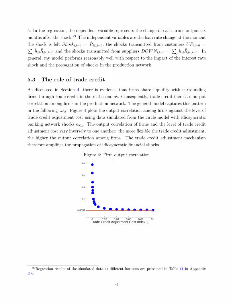
5.3 The role of trade credit

As discussed in Section 4, there is evidence that firms share liquidity with surrounding

firms through trade credit in the real economy. Consequently, trade credit increases output

correlation among firms in the production network. The general model captures this pattern

in the following way. Figure 4 plots the output correlation among firms against the level of

trade credit adjustment cost using data simulated from the circle model with idiosyncratic

banking network shocks εNei . The output correlation of firms and the level of trade credit

adjustment cost vary inversely to one another: the more flexible the trade credit adjustment,

the higher the output correlation among firms. The trade credit adjustment mechanism

therefore amplifies the propagation of idiosyncratic financial shocks.

Figure 4: Firm output correlation

Trade Credit Adjustment Cost Index &0 0.02 0.04 0.06 0.08 0.1

0.5052

0.6

0.7

0.8

0.9firm output correlation

29Regression results of the simulated data at different horizons are presented in Table 11 in AppendixD.6.

31

5.4 Amplification effect of the network structure

After confirming that the general model could capture empirical patterns presented in Section

3, I proceed to calibrate the model fully using the 14-sector data in Table 4. I begin by

comparing the network model with a representative firm model. Consider a representative

firm model with the same type of financial frictions described in Section 4. The parameters in

this economy are calibrated using data in Table 3 and the last row of Table 4. As illustrated

in Figure 5, the sensitivity of aggregate variables to shocks is very different in these two types

of economies. Figure 5 plots the impulse responses of aggregate output Y , consumption C,

investment I and premium (E(Rik)−R) after an aggregate banking net worth Ne shock, an

aggregate technology shock z, a capital quality shock ξ and monetary policy shock i.30 Ne

shock is an unanticipated negative 1% reduction in the existing banker’s net worth within

each sector. The technology z shock is a negative 1% innovation in TFP of each sector,

which is an AR1 process with autocorrelation 0.95. ξ shock is a negative 1% change in

capital quality of each sector and is AR1 with autocorrelation 0.66. Monetary policy i shock

is an unanticipated 10 basis-point increase in the short-term interest rate.

Remarkably, the input-output structure generates an amplification effect on the aggregate

impact of shocks. Compared with a representative firm model (indicated by the dashed black

line), a network economy (indicated by the solid red line) is more responsive to all manner

of shocks. Consider, for example, an aggregate banking net worth shock: the responses of

the premium (E(Rk) − R) in these two types of models are not significantly different from

each other. Because the financial intermediaries have the same type of horizontal structure

in these two models, a uniform contraction of Ne impacts the interest rate Rk and RL

through the same mechanism within each banking sector. Consequently, the responses of

the premium are similar. Nonetheless, the response of Y in the network model is more than

two times stronger than it is in a representative firm model. Unlike bankers, firms in the

network economy are interconnected. The input-output linkages among firms amplify the

negative impact of the high borrowing cost and the liquidity shock. Similarly, the technology

or capital quality shocks propagate upstream and downstream in the production network and

ultimately affect aggregate output. The network structure amplifies the aggregate impact of

the shock.

30(E(Rk) − R) is calculated as the average premium across sectors; I is the total investment in theeconomy.

32

Figure 5: Aggregate variables response to banking net worth (Ne), technology (z), capitalquality (ξ) and monetary (i)

20 40

bank

net

wor

th

#10-3

-2

-1

0Y

20 40

#10-4

-15

-5

5

C

20 40

#10-3

-10

-5

0

I

20 40

#10-4

0

4

8E(R

k)-R

20 40

tech

nolo

gy

-0.02

-0.01

0Y

20 40-0.015

-0.01

0C

20 40

-0.06

-0.03

0I

20 40

#10-4

0

10

20E(R

k)-R

20 40

capi

tal q

ualit

y

-0.05

-0.025

0Y

20 40

-0.06

-0.03

0C

20 40

-0.1

0

0.1I

20 40

#10-3

0

3

6

E(Rk)-R

Quarters20 40

mon

etar

y po

licy

#10-3

-2

-1

0Y

Quarters20 40

#10-4

-10

-5

0

C

Quarters20 40

#10-3

-10

-5

0

I

Quarters20 40

#10-4

0

5

E(Rk)-R

-­‐4.0E-­‐04

-­‐3.5E-­‐04

-­‐3.0E-­‐04

-­‐2.5E-­‐04

-­‐2.0E-­‐04

-­‐1.5E-­‐04

-­‐1.0E-­‐04

-­‐5.0E-­‐05

0.0E+00 1 2 3 4 5

output (with trade credit adjustment)

fix tc high cost mid cost low cost

Representative Firm Model Network

33

6 Credit Policy Implication

Suppose that, during a severe financial crisis, a policymaker is willing to facilitate lending.

Let Spit and Lpit be the value of assets intermediated by the financial intermediaries, and let Sgit

and Lgit be the value of assets intermediated by the government. Under these circumstances,

the total value of intermediated assets of sector i is,

Sit = Spit + Sgit,

Lit = Lpit + Lgit.

To facilitate lending, the policymaker issues government debt to households that pay the

riskless rate Rt, and it lends funds to non-financial firms at the banking credit rate RiLt.

For the policymaker, unlike for the financial intermediaries, there are no frictions on issuing

debt and purchasing private assets. Whereas there are N types of assets according to the

issuing sector, the policymaker is flexible in targeting liquidities. The policymaker could

then either lend funds to all sectors proportionally (according to their market size), or could

target liquidity to specific sectors. The total value of assets intermediated by the government

would be,

CPt =N∑i

CPit =N∑i

(QitSgit + Lgit) (33)

Suppose the credit policy follows that

CPt+1 = ρCPCPt + εCPt+1, with εCPt = −ϑεNet , (34)

where ϑ is a constant and εNet is the banking net worth shock. Accordingly, the total value

of assets intermediated by the policymaker would be proportional to the contraction of the

banking net worth, and CPt follows an AR1 process. Moreover, following Gertler and Karadi

(2011), this central bank intermediation involves the loss of efficiency; specifically, there is

an efficiency cost of o for every unit of central bank credit that is supplied.

I compare credit policies by targeting liquidity to different sectors. Let YCPoni denote the

aggregate output change after an aggregate financial shock (Ne shock) and a sector-specific

credit policy shock (i.e. CPt = CPit, CPjt = 0,∀j 6= i). The comparison of YCPoni across i

makes clear which sector i the central bank should target with loans during the crisis.

I simulate the model with ϑ = 5% and o = 0.01. Figure 6 plots the response of the

aggregate output and the premium after a -1% Ne shock and a credit policy targeting

the real estate sector. Compared with an economy that lacks credit policies, this economy

34

Figure 6: Aggregate variables response to banking net worth (Ne) and credit policy (CP )shocks

10 20 30 40

#10-3

-2.5

-2

-1.5

-1

-0.5

0aggregate output Y

without credit policy target credit policy to sector i20 40

#10-4

0

2

4

6

risk premium E(Rk)-R

Ne shock is a negative 1% change in the banking net worth of each sector. Credit policy is a 5% of the Neshock targeting real estate with a quarterly autoregressive factor of 0.8.

Figure 7: YCPoni

(a) Contemporaneous response

Upstreamness1 2 3 4

#10-4

-6

-5

-4

-3

-2

AgricultureMining

Utility

Construction

ManufacturingWholesale

Retail Transportation

InformationReal Estate

Professrional business services

Education

ArtsOther services

(b) 2-year cumulative change

Upstreamness1 2 3 4

-0.016

-0.015

-0.014

-0.013

-0.012

Agriculture

MiningUtility

Construction

Manufacturing

Wholesale

RetailTransportation

Information

Real Estate

Professrional business services

Education

Arts

Other services

In panel (a) contemporaneous response, each red dot represents YCPoni upon the impact of the Neand credit policy shocks. The real estate dot corresponds the cross point of the red curve with they-axis in the left panel of Figure 6. In panel (b) 2-year cumulative change, each red dot represents∑t=8

t=0 YCPoni,t. The real estate dot corresponds to the size of the pink area in the left panel ofFigure 6.

35

experiences less output contraction and a smaller premium increase.

Given that government has the ability to target liquidity to different sectors, the question

arises as to which sector or sectors should be treated as priorities following aggregate financial

shocks.31 Figure 7 plots YCPoni in the short run and in the long run against the relative

upstreamness of each sector.32 It turns out that credit policies have greater impact when

liquidity is supplied to downstream sectors, which is not surprising, given that financial

shocks propagate upstream. Moreover, this result is consistent with Proposition 3 that the

financial condition of the downstream sector is more important systemically.

7 Conclusions

This paper investigates how the interaction between the production network and trade credit

network affect the propagation of financial shocks. Using the U.S. input-output matrix and

the bond yield data, I find strong upstream propagation of financial shocks. A 1% increase

in the bond yield of one sector’s customers (weighted by their input-output linkages) could

impact the focal sector’s output by -0.17%. To capture this pattern in an input-output model,

it has been shown to be important to introduce financial friction in trade and interlocked

balance sheets of trading parties. I have incorporated financial frictions and the trade credit

network into an input-output model and have thereby been able to generate quantitative

predictions consistent with my empirical findings. In addition, I have demonstrated that

credit policies have a greater impact when liquidity is supplied to downstream sectors after

an aggregate liquidity shock. For downstream sectors are more important systemically, given

that financial shocks propagate upstream.

This paper represents the first theoretical study to introduce a trade credit network into

an input-output model within a general equilibrium framework. Financial market loans and

trade credit are the two most important sources of external finance for firms. Through

the trade credit mechanism, each firm shares liquidity with surrounding firms, and as a

consequence idiosyncratic shocks spread through trade and financial linkages of firms.

My findings here may serve to stimulate further research. Thus, for example, interesting

results might be observed in a model based on a micro-founded trade credit structure. If one

31I focus on the credit policy implications after those of aggregate financial shocks, where the liquiditycontraction across sectors is uniformly distributed. In the case of unbalanced financial shocks across sectors,it is obvious that the policymaker should supply liquidity to sectors that have experienced the strongestliquidity shock.

32Different measures of the long run change of YCPoni have been examined. For example, the scatter plotof the 10-year cumulative change of YCPoni and the upstreamness of sectors behaves in a manner qualitativelysimilar to that found in Panel (b) of Figure 7. The 2-year cumulative change of YCPoni corresponds to thetotal size of the pink and green areas in the left panel of Figure 6.

36

were to allow a trade credit default, a strong liquidity shock to one firm could cause a cascade

of defaults throughout the trade credit network, setting off an avalanche of production failure

and generating a persistent aggregate output contraction. The work discussed here also

suggests that inter-bank lending could play an important role in recovery from idiosyncratic

shocks. In reality, there exists both a complicated production network and an entangled

financial network. An idiosyncratic financial shock not only transfers through the input-

output network, but also spills over in the banking network. It is my hope that this paper

will encourage further theoretical and empirical studies on the role of financial frictions in

the input-output economy.

37

References

Acemoglu, Daron, Ufuk Akcigit, and William Kerr (2015a), “Networks and the macroecon-

omy: An empirical exploration.” NBER Macro Conference.

Acemoglu, Daron, Vasco M. Carvalho, Asuman Ozdaglar, and Alireza Tahbaz-Salehi (2012),

“The network origins of aggregate fluctuations.” Econometrica, 80.

Acemoglu, Daron, Asuman Ozdaglar, and Alireza Tahbaz-Salehi (2015b), “Networks, shocks,

and systemic risk.” In The Oxford Handbook on the Economics of Networks (Yann

Bramoulle, Andrea Galeotti, and Brian Rogers, eds.), Oxford University Press, Oxford.

Acemoglu, Daron, Asuman Ozdaglar, and Alireza Tahbaz-Salehi (2015c), “Systemic risk and

stability in financial networks.” American Economic Review, 105.

Allen, Franklin and Douglas Gale (2000), “Financial contagion.” Journal of Political Econ-

omy, 108.

Bak, Per, Kan Chen, Jose Scheinkman, and Michael Woodford (1993), “Aggregate fluctua-

tions from independent sectoral shocks: self-organized criticality in a model of production

and inventory dynamics.” Ricerche Economiche, 47, 3–30.

Baqaee, David R. (2015), “Cascading failures in production networks.” Working paper.

Bigio, Saki and Jennifer La’O (2013), “Financial frictions in production networks.” Working

paper.

Boissay, Frederic and Reint Gropp (2007), “Trade credit defaults and liquidity provision by

firms.” European Central Bank, Working Paper Series No. 753.

Burkart, Mike and Tore Ellingsen (2004), “In-kind finance: A theory of trade credit.” Amer-

ican Economic Review, 94.

Carvalho, Vasco M. and Xavier Gabaix (2013), “The great diversification and its undoing.”

American Economic Review, 103.

Chodorow-Reich, Gabriel (2014), “The employment effects of credit market disruptions:

Firm-level evidence from the 20089 financial crisis.” The Quarterly Journal of Economics,

129.

Conley, Timothy G. and Bill Dupor (2003), “A spatial analysis of sectoral complementarity.”

Journal of Political Economy, 111.

38

Cunat, Vicente (2007), “Trade credit: Suppliers as debt collectors and insurance providers.”

Review of Financial Studies, 20, 491–527.

Curdia, Vasco and Michael Woodford (2011), “The central-bank balance sheet as an instru-

ment of monetary policy.” Journal of Monetary Economics, 58, 54–79.

di Giovanni, Julian, Andrei A. Levchenko, and Isabelle Mejean (2014), “Firms, destinations,

and aggregate fluctuations.” Econometrica, 82, 13031340.

Dupor, Bill (1999), “Aggregation and irrelevance in multi-sector models.” Journal of Mon-

etary Economics, 43.

Foerster, Andrew T., Pierre-Daniel G. Sarte, and Mark W. Watson (2011), “Sectoral ver-

sus aggregate shocks: A structural factor analysis of industrial production.” Journal of

Political Economy, 119, 1–38.

Gabaix, Xavier (2011), “The granular origins of aggregate fluctuations.” Econometrica, 79.

Gao, Janet (2014), “Business networks, firm connectivity, and firm policies.” Working paper.

Gertler, Mark and Peter Karadi (2011), “A model of unconventional monetary policy.”

Journal of Monetary Economics, 58, 17–34.

Hertzel, Michael G., Zhi Li, Micah S. Officer, and Kimberly J. Rodgers (2008), “Officer

and inter-firm linkages and the wealth effects of financial distress along the supply chain.”

Journal of Financial Economics, 87, 374–387.

Horvath, Michael (1998), “Cyclicality and sectoral linkages: aggregate fluctuations from

independent sectoral shocks.” Review of Economic Dynamics, 1.

Horvath, Michael (2000), “Sectoral shocks and aggregate fluctuations.” Journal of Monetary

Economics, 45.

Hulten, Charles R. (1978), “Growth accounting with intermediate inputs.” The Review of

Economic Studies, 45.

Jones, Charles I. (2011), “Intermediate goods and weak links: A theory of economic devel-

opment.” American Economic Journal: Macroeconomics, 3, 1–28.

Jones, Charles I. (2012), “Misallocation, economic growth, and input-output economics.” In

Advances in Economics and Econometrics (M. Arellano D. Acemoglu and E. Dekel, eds.),

Cambridge University Press, New York.

39

Jovanovic, Boyan (1987), “Micro shocks and aggregate risk.” Quarterly Journal of Eco-

nomics, 102.

Kalemli-Ozcan, Sebnem, Hyun Song Shin Se-Jik Kim, Bent E. Sørensen, and Sevcan Yesiltas

(2012), “Financial shocks in production chains.” Unpublished manuscript.

Kiyotaki, Nobuhiro and John Moore (1997), “Credit chains.” Unpublished manuscript.

Long, John B. and Charles I. Plosser (1983), “Real business cycles.” Journal of Political

Economy, 91.

Nilsen, Jeffrey H. (2002), “Trade credit and the bank lending channel.” Journal of Money,

Credit and Banking, 34.

Peterson, Michell A. and Raghuram G. Rajan (1997), “Trade credit: Theories and evidence.”

Review of Financial Studies, 10.

Price, David A. (2012), “When the fed conducts credit policy.” Federal Reserve Region

Focus.

Raddatz, Claudio (2008), “Credit chains and sectoral comovement: Does the use of trade

credit amplify sectoral shocks?” Policy Research Working Paper Series 4525, The World

Bank.

Reis, Ricardo (2009), “Interpreting the unconventional u.s. monetary policy of 2007-09.”

Brookings Papers on Economic Activity, 40, 119–165.

Shea, John (2002), “Complementarities and comovements.” Journal of Money, Credit, and

Banking, 34, 412433.

Su, Hsuan-Li (2014), “Financial frictions, capital misallocation, and input-output linkages.”

Working paper.

40

A Appendix: Trade Credit

Trade credit is a short-term loan a supplier provides to its customer upon a purchase of its

product. It is the single most important source of external finance for firms (Boissay and

Gropp (2007)). Two types of trade credit rules are common (Nilsen (2002)). One type is a

one part contract, Net-30. Suppliers give buyer 30-day interest free loans. The other type

is a two part contract, 2/10 Net 30. If customers pay within 10 days of delivery, then they

qualify a 2% discount; otherwise they can pay up to 30 days after delivery.

Empirical evidence shows that the implicit interest rate in a trade credit agreement is

usually very high as compared with the rate on bank credit.33 Peterson and Rajan (1997) for

example, conservatively estimate trade credit cost and find it more expensive than 99.8% of

the loans. The high interest rate on trade credit arises because of an insurance premium and

a default premium. Suppliers provide financing help through trade credit or defer payments

when customers have already exhausted their bank credit line. In my model, I do not consider

trade credit interests. However, my results about the propagation of financial shocks still

hold in a set up with positive trade credit interest rates.

Several theories have been put forth to explain why suppliers provide credit to customers

even though those firms cannot get additional banking credit. On the one hand, suppliers

would like to keep business relationship as the cost of losing customers is high. On the other

hand, suppliers may have an information advantage over banks and have a comparative ad-

vantage in liquidating collateral that the borrower may put up to secure the loan. Moreover,

the transaction argument states that trade credit reduces the transaction cost of paying bills.

Also, there are papers study the role of trade credit in mitigating supply chain moral hazard.

This paper does not focus on explaining the existence and the optimal choice of trade credit,

but it studies the impact of trade credit on the propagation of shocks.

Notably, a trade credit debtor in bankruptcy almost surely default on the claims held by

its trade creditors (Boissay and Gropp (2007)). Shocks to the liquidity of some firms caused

by the default of the customers, may in turn cause default or postponement of accounts

payables on their suppliers and propagate upstream through the production chain. A distress

at a single firm may induce a cascade of defaults throughout the production chain. The trade

credit propagation mechanism will amplify the impact of idiosyncratic shocks on aggregate

output. Thus, this mechanism creates a big multiplier effect. Although this feature is not

included in this paper, it is worth investigating in my future research.

33Be aware that price may be in the form of intrinsic interest.

41

Table 6: Trade Credit (Compustat)

AP/COGS AP/S AR/S AP/TA AR/TAAgriculture 0.43 0.30 0.41 0.05 0.04Mining 1.00 0.50 0.60 0.05 0.05Utilities 0.49 0.36 0.51 0.04 0.06Construction 0.43 0.34 0.88 0.10 0.20Manufacturing 0.49 0.32 0.57 0.07 0.13Wholesale trade 0.44 0.33 0.41 0.18 0.21Retail trade 0.42 0.28 0.09 0.14 0.05Transportation 0.30 0.22 0.37 0.04 0.09Information 0.64 0.26 0.57 0.05 0.09FIRRL 60.42 25.68 0.68 0.56 0.07PBS 0.37 0.23 0.66 0.06 0.20Educational 0.25 0.16 0.57 0.05 0.15Arts 0.21 0.15 0.05 0.04 0.01Other services 0.37 0.23 0.22 0.06 0.07

Table 7: Trade Credit (QFR)

AP/S AR/S AP/TA AR/TAMining 0.49 0.64 0.05 0.06Manufacturing 0.31 0.45 0.07 0.10Wholesale trade 0.33 0.36 0.20 0.22Retail trade 0.28 0.14 0.16 0.08

42

B Appendix: Simple Network Models

B.1 Equilibrium results

The horizontal economy:

Notably, the labor demand function in this economy follows,

αipimi = Riwli, i ∈ 1, 2, 3. (35)

The equilibrium output of firms are functions of their own technology level zi and the interest

rate Ri, i.e.

mhi = zi(R

−1i αiζ

hi )αi , i ∈ 1, 2, 3. (36)

The equilibrium aggregate output becomes,

Y h = Ξ(mh1)ζ

h1 (mh

2)ζh2 (mh

3)ζh3 (37)

The network economy:

The equilibrium sectoral outputs of the TC-network economy are,

m1 =z1

R1

ζ1 + (1− α2)

[θ2 + (1− θ2)R1]

[θ2 + (1− θ2)R2]

[ζ2 + (1− α3)ζ3

[θ3 + (1− θ3)R2]

[θ3 + (1− θ3)R3]

](38)

m2 = z2z1−α21 αα2

2 (1− α2)1−α2R−(1−α2)1 R−α2

2([θ2 + (1− θ2)R1]

[θ2 + (1− θ2)R2]

)1−α2[ζ2 + (1− α3)ζ3

[θ3 + (1− θ3)R2]

[θ3 + (1− θ3)R3]

](39)

m3 = z3z1−α32 z

(1−α2)(1−α3)1 αα3

3 (1− α3)1−α3αα2(1−α3)2 (1− α2)(1−α2)(1−α3)ζ3R

−(1−α2)(1−α3)1 R

−α2(1−α3)2 R−α3

3([θ2 + (1− θ2)R1]

[θ2 + (1− θ2)R2]

)(1−α2)(1−α3)([θ3 + (1− θ3)R2]

[θ3 + (1− θ3)R3]

)1−α3

(40)

The labor allocation is,

l1 =

ζ1 + (1− α2)

[θ2 + (1− θ2)R1]

[θ2 + (1− θ2)R2]

[ζ2 + (1− α3)ζ3

[θ3 + (1− θ3)R2]

[θ3 + (1− θ3)R3]

]· α1

R1

, (41)

l2 =

ζ2 + (1− α3)ζ3

[θ3 + (1− θ3)R2]

[θ3 + (1− θ3)R3]

· α2

R2

, (42)

l3 = ζ3 ·α3

R3

, (43)

43

The aggregate output is,

Y = ΘzV11 zV22 zV33 R−V11 R−α2V22 R−α3V3

3([θ2 + (1− θ2)R1]

[θ2 + (1− θ2)R2]

)V1−ζ1 ( [θ3 + (1− θ3)R2]

[θ3 + (1− θ3)R3]

)V2−ζ2. (44)

B.2 Propagation of Shocks

B.2.1 Supply shocks

I begin the analysis of supply shocks by analyzing their transmission. In particular, I want to

consider technology shocks in the network economy. Clearly, the technologies employed by

upstream firms have significant impact on the outputs of their downstream firms (according

to Equation 38-40).

Proposition 5. In the network model with financial frictions, supply shocks generate strong

downstream propagation. Moreover, downstream firms with larger shares of intermediate

inputs (1−αi+1) are more affected by this downstream propagation. The elasticity of sectoral

output with respect to the technology of firm 2 (z2) is,

∂m1

∂z2

z2

m1

= 0,∂m2

∂z2

z2

m2

= 1,∂m3

∂z2

z2

m3

= (1− α3),

Technology shocks mainly generate downstream propagation because they lead to sig-

nificant changes in intermediate input prices. Moreover, the share of intermediate inputs

in the production function ((1 − αi)) controls the power of this downstream propagation.

Intuitively, the larger the intermediate input usage of a firm, the more sensitive the firm is

to shocks that flow down the production chain.

B.2.2 Demand shocks

To explain the propagation of demand shocks in a production chain, I modify the non-

production side of the model slightly, as follows: 1) the aggregate consumption of households

is measured as a composite of the three specialized products: C = cζ11 cζ22 c

ζ33 ; 2) a government

that collects lump-sum taxes to finance its expenditures g1, g2, g3 is posited. The budget

constraints of households thus become∑

i pici + T = wL+ Ψ. The budget constraint of the

government becomes∑

i pigi = T . The market clearing conditions become

m1 = m21 + c1 + g1, m2 = m32 + c2 + g2, m3 = c3 + g3.

44

By the zero profit condition,

p1 =w

z1

,

p2 =1

z2

(1

α2

)α2(

1

1− α2

)(1−α2)

wα2p(1−α2)1 ,

p3 =1

z3

(1

α3

)α3(

1

1− α3

)(1−α3)

wα3p(1−α3)2 .

Normalize w to be 1. I have sectoral prices, p1, p2, p3 are independent of the demand shock.

Consumption c1, c2, c3 is independent of the demand shock. m3 doesn’t change. ∆m2

equals ∆g2.

From this starting point, the impact of demand shocks such as government expenditure

shocks (gi shocks) to the economy can be analyzed. Solving for the equilibrium of this

economy generates the following result.

Proposition 6. In the network model, when government expenditure is taken into account,

demand shocks generate strong upstream propagation. Moreover, firms that have a larger

proportion of output purchased by the impacted firms (ρi ≡ mi+1,i

mi) are naturally more sen-

sitive to the demand shock. The sensitivity of firm outputs to the government expenditure

shock to product 2 (g2) is,

∂m1

∂g2

= f(ρ1),∂m2

∂g2

= 1,∂m3

∂g2

= 0,

with ∂f(ρ1)∂ρ1

> 0.

Consumption and price levels of the economy remain constant. The affected firms adjust

their production levels, and thus their input demands, after the government expenditure

shock. As a consequence, demand-side shocks mainly create upstream propagation. More-

over, the share of sectoral output used as intermediate inputs ρi governs the strength of this

upstream propagation. Intuitively, the larger this share is, the more sensitive the firm is to

shocks that flow up the production chain.

45

B.2.3 Financial shocks

The elasticities of sectoral output with respect to the interest rate of firm 2 (R2) are,

∂m1

∂R2

R2

m1

=(1− α2)ζ2[θ2 + (1− θ2)R1]

[θ2 + (1− θ2)R2]2

[−(1− θ2) + (1− α3)ζ3

θ2−θ3[θ3+(1−θ3)R3]

]R2

ζ1 + (1− α2) [θ2+(1−θ2)R1][θ2+(1−θ2)R2]

[ζ2 + (1− α3)ζ3

[θ3+(1−θ3)R2][θ3+(1−θ3)R3]

]∂m2

∂R2

R2

m2

= −α2 − (1− α2)(1− θ2)R2

θ2 + (1− θ2)R2

+(1− α3)ζ3(1− θ3)R2

ζ2 + (1− α3)ζ3θ3+(1−θ3)R2

θ3+(1−θ3)R3

,

∂m3

∂R2

R2

m3

= −(1− α3)

[α2 + (1− α2)

(1− θ2)R2

θ2 + (1− θ2)R2

− (1− θ3)R2

θ3 + (1− θ3)R2

].

If θi = 0,∀i,

∂m1

∂R2

R2

m1

= −(1− α2)ζ2z1Υ1

R2m1

,∂m2

∂R2

R2

m2

= −ζ2z2z1−α21 Υ2

R2m2

,∂m3

∂R2

R2

m3

= 0.

If θi = 1,∀i,

∂m1

∂R2

R2

m1

= 0,∂m2

∂R2

R2

m2

= −α2,∂m3

∂R2

R2

m3

= −α2(1− α3).

B.3 The influence vector

Proof of Proposition 3. By the zero profit condition,

pi = ααii (1− αi)1−αiΠ(ωij)ωij(1−αi) 1

ziwαiRαi

i ΠNj=1

(pj

[(1− θi)Ri + θi]

[(1− θi)Rj + θi]

)ωij(1−αi).

Log linearize:

αiw = zi + pi − (1− αi)∑

ωij pj

−[αi + (1− αi)

(1− θi)R[(1− θi)R + θi]

]Ri + (1− αi)

(1− θi)R[(1− θi)R + θi]

∑ωijRj.

Define the following vectors,

z =

z1

z2

...

zN

, R =

R1

R2

...

RN

, p =

p1

p2

...

pN

Ω =

(1− α1)ω11 (1− α1)ω12 · · · (1− α1)ω1N

(1− α2)ω21 (1− α2)ω22 · · · (1− α2)ω2N

......

. . ....

(1− αN)ωN1 (1− αN)ωN2 · · · (1− αN)ωNN

46

I1 =

α1 + (1− α1) (1−θ1)R

[(1−θ1)R+θ1]0 · · · 0

0 α2 + (1− α2) (1−θ2)R

[(1−θ2)R+θ2]· · · 0

......

. . ....

0 0 · · · αN + (1− αN) (1−θN )R

[(1−θN )R+θN ]

I2 =

(1−θ1)R

[(1−θ1)R+θ1]0 · · · 0

0 (1−θ2)R

[(1−θ2)R+θ2]· · · 0

......

. . ....

0 0 · · · (1−θN )R

[(1−θN )R+θN ]

Assume αi = αj, thus

α1w = z− [I1 − I2Ω]R + (I − Ω)p,

where 1 is a column vector of N ones.

Multiplying this equation by ((I − Ω′)−1ζ)′ obtains

w = v′[z− (I1 − I2Ω)R].

with

v ≡ (I − Ω′)−1ζ.

ζ ′p corresponds to the aggregate price index P , which is constant.

From households’ optimization problem, we have Y = w. Thus,

Y = v′[z− (I1 − I2Ω)R].

Solve yi and mi. Henceforth, I solve for yi and mi. From firms’ first order conditions I

obtain,(1− θij)Ri + θij(1− θij)Rj + θij

pjmij = (1− αi)ωijpimi,

wliRi = αipimi.

From the final producer’s first order conditions I have,

piyi = ζiY = ζiw.

47

Log linearize the production function and substitute the first three equations, I obtain,

mi = zi + αi(mi + pi − w − Ri) + (1− αi)∑j

ωij[mi + pi − pj

− (1− θi)R[(1− θi)R + θi]

Ri +(1− θi)R

[(1− θi)R + θi]Rj],

⇒

0 = zi + αi(−yi − Ri) + (1− αi)∑j

ωij

yj − yi −

(1− θi)R[(1− θi)R + θi]

Ri +(1− θi)R

[(1− θi)R + θi]Rj

.

Thus,

y = [I − Ω]−1[z− (I1 − I2Ω)]R,

where y is a vector of yi.

From goods market clearing condition, I obtain

mi = yi +∑j

mji

= yi +∑j

(1− αj)ωjimjyiyj

ζjζi

[(1− θj)Ri + θj]

[(1− θj)Rj + θj],

ζimi

yi= ζi +

∑j

(1− αj)ωjiζjmj

yj

[(1− θj)Ri + θj]

[(1− θj)Rj + θj].

Denote ti = miyi

, I obtain

ζititi =∑j

(1− αj)ωjiζj tj[tj +

(1− θj)R[(1− θj)R + θj]

(Ri − Rj)

].

Further replace ωji by ωji ≡ 11−αj

mjipjimipi

= ωjimj pjmipi

, then34

ti =∑j

(1− αj)ωji[tj +

(1− θj)R[(1− θj)R + θj]

(Ri − Rj)

].

34Notice that at ωji = 11−αj

mjipjimj pj

.

48

Denote,

Ω =

(1− α1)ω11 (1− α1)ω12 · · · (1− α1)ω1N

(1− α2)ω21 (1− α2)ω22 · · · (1− α2)ω2N

......

. . ....

(1− αN)ωN1 (1− αN)ωN2 · · · (1− αN)ωNN

Thus

t = [I − Ω′]−1[I∑ − Ω′I2]R,

where I∑ is a diagonal matrix with diagonal element∑

j(1− αj)ωji(1−θj)R

[(1−θj)R+θj ]. Given that,

ti = mi − yi, so t = m− y.

Thus, the vector of the log deviation of firm output from the steady state (mi) follows,

m = [I − Ω]−1z−

[I − Ω′]−1[−I∑ + Ω′I2] + [I − Ω]−1(I1 − I2Ω)]

R. (45)

The first term in the brace captures upstream propagation of the interest rate shock, while the

second term captures downstream propagation. This equation indicates that financial shocks

propagate both upstream and downstream, while supply side shocks (such as technology

shocks) only propagate downstream.

C Appendix: Empirical Results & Robustness Checks

C.1 The U.S. input-output matrix

Figure 8 plots the input-output matrix (Ω) of the U.S..

C.2 Empirical results

49

Figure 8: The U.S. Input-Output Matrix

Destination Industry (Output)

AgricultureMining

Utility

Construction

Manufacturing

WholesaleRetail

Transportation

Information

FinanInsurRealEstate

ProfBusiServ

EducationArts

OtherServices

Government

Sup

plie

rs (

Inpu

t)

Government

OtherServices

Arts

Education

ProfBusiServ

FinInsurRealEst

Information

Transportation

Retail

Wholesale

Manufacturing

Construction

Utility

Mining

AgricultureInput-Output Matrix

Table 8: UP vs. DOWN - panel

dependent variable: mit (2002.09-2014.12)(1) (2) (3) (4)monthly quarterly 6-month yearly

UPit−1 -0.0876** -0.1704*** -0.0929** -0.1108*[0.0338] [0.0301] [0.0441] [0.0564]

DOWNit−1 0.0479 0.1779 0.1645 0.0374[0.0605] [0.1252] [0.1687] [0.1927]

Shockit−1 0.0685 -0.0917 -0.4395*** -0.2775**[0.0480] [0.1058] [0.1221] [0.1230]

mit−1 -0.1270*** 0.0027 0.0891* -0.0851[0.0358] [0.0424] [0.0502] [0.0701]

Observations 8,673 2,832 1,357 649Group 59 59 59 59

Notes: Estimations include time and sector fixed effects, report stan-dard errors clustered by sector and are unweighted. ∗, ∗∗, and ∗∗∗

indicate statistical significance at the 10%, 5%, and 1% levels re-spectively.

50

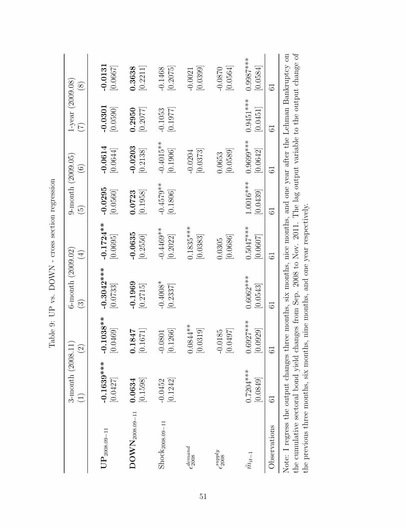
Tab

le9:

UP

vs.

DO

WN

-cr

oss

sect

ion

regr

essi

on

3-m

onth

(200

8.11

)6-

mon

th(2

009.

02)

9-m

onth

(200

9.05

)1-

year

(200

9.08

)(1

)(2

)(3

)(4

)(5

)(6

)(7

)(8

)

UP

2008.0

9−

11

-0.1

639***

-0.1

038**

-0.3

042***

-0.1

724**

-0.0

295

-0.0

614

-0.0

301

-0.0

131

[0.0

427]

[0.0

469]

[0.0

733]

[0.0

695]

[0.0

560]

[0.0

644]

[0.0

590]

[0.0

667]

DO

WN

2008.0

9−

11

0.0

634

0.1

847

-0.1

969

-0.0

635

0.0

723

-0.0

203

0.2

950

0.3

638

[0.1

598]

[0.1

671]

[0.2

715]

[0.2

550]

[0.1

958]

[0.2

138]

[0.2

077]

[0.2

211]

Shock

2008.0

9−

11

-0.0

452

-0.0

801

-0.4

008*

-0.4

469*

*-0

.457

9**

-0.4

015*

*-0

.105

3-0

.146

8[0

.124

2][0

.126

6][0

.233

7][0

.202

2][0

.180

6][0

.190

6][0

.197

7][0

.207

5]

εdem

and

2008

0.08

44**

0.18

35**

*-0

.020

4-0

.002

1[0

.031

9][0

.038

3][0

.037

3][0

.039

9]

εsupply

2008

-0.0

185

0.03

050.

0653

-0.0

870

[0.0

497]

[0.0

686]

[0.0

589]

[0.0

564]

mit−

10.

7204

***

0.69

27**

*0.

6062

***

0.50

47**

*1.

0016

***

0.96

99**

*0.

9451

***

0.99

87**

*[0

.084

9][0

.092

9][0

.054

3][0

.060

7][0

.043

9][0

.064

2][0

.045

1][0

.058

4]

Obse

rvat

ions

6161

6161

6161

6161

Not

e:I

regr

ess

the

outp

ut

chan

ges

thre

em

onth

s,si

xm

onth

s,nic

em

onth

s,an

don

eye

araf

ter

the

Leh

man

Ban

kru

ptc

yon

the

cum

ula

tive

sect

oral

bon

dyie

ldch

ange

sfr

omSep

.20

08to

Nov

.20

11.

The

lag

outp

ut

vari

able

toth

eou

tput

chan

geof

the

pre

vio

us

thre

em

onth

s,si

xm

onth

s,nin

em

onth

s,an

don

eye

arre

spec

tive

ly.

51

Table 10: UP vs. DOWN: additional lags

dependent variable: mit (2002.09-2014.12)(1) (2) (3) (4)monthly quarterly 6-month yearly

L.upshock -0.0557 -0.1963*** -0.1029** -0.0985*[0.0358] [0.0343] [0.0415] [0.0576]

L2.upshock -0.0905** 0.0281 -0.0612 0.0454[0.0352] [0.0341] [0.0421] [0.0392]

L.downshock 0.0428 0.2187 0.1686 0.0610[0.0670] [0.1327] [0.1747] [0.2002]

L2.downshock -0.1389** -0.1045 -0.0254 -0.0164[0.0655] [0.1106] [0.1149] [0.1471]

L.ownshock 0.0479 -0.0641 -0.4374*** -0.3317**[0.0489] [0.1189] [0.1238] [0.1362]

L2.ownshock 0.0778 -0.2173** -0.0790 -0.1668[0.0659] [0.0859] [0.0902] [0.1218]

L.dip -0.0078 0.0087 -0.0804** -0.0473[0.0277] [0.0412] [0.0364] [0.0418]

L2.dip -0.1306*** 0.0394 0.0768 -0.1039[0.0385] [0.0291] [0.0509] [0.0724]

Observations 8,673 2,832 1,357 649Group 59 59 59 59

Notes: Estimations include time and sector fixed effects, reportstandard errors clustered by sector and are unweighted. ∗, ∗∗, and∗∗∗ indicate statistical significance at the 10%, 5%, and 1% levelsrespectively.

52

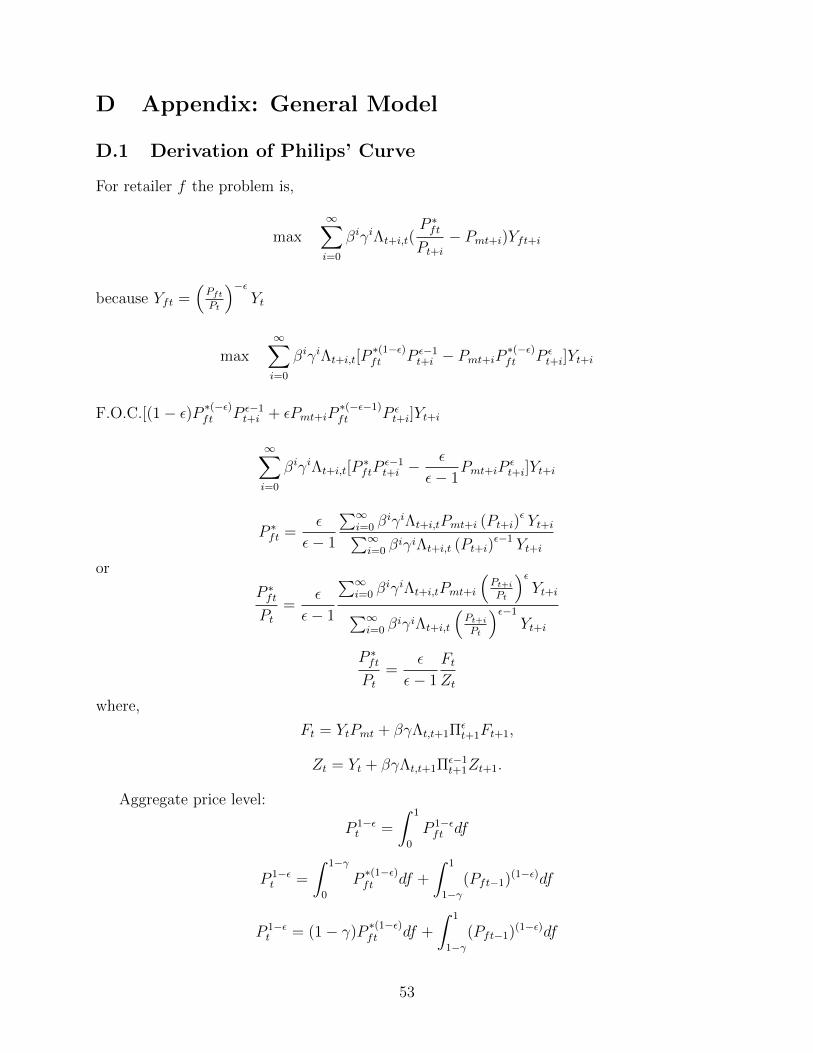
D Appendix: General Model

D.1 Derivation of Philips’ Curve

For retailer f the problem is,

max∞∑i=0

βiγiΛt+i,t(P ∗ftPt+i

− Pmt+i)Yft+i

because Yft =(PftPt

)−εYt

max∞∑i=0

βiγiΛt+i,t[P∗(1−ε)ft P ε−1

t+i − Pmt+iP∗(−ε)ft P ε

t+i]Yt+i

F.O.C.[(1− ε)P ∗(−ε)ft P ε−1t+i + εPmt+iP

∗(−ε−1)ft P ε

t+i]Yt+i

∞∑i=0

βiγiΛt+i,t[P∗ftP

ε−1t+i −

ε

ε− 1Pmt+iP

εt+i]Yt+i

P ∗ft =ε

ε− 1

∑∞i=0 β

iγiΛt+i,tPmt+i (Pt+i)ε Yt+i∑∞

i=0 βiγiΛt+i,t (Pt+i)

ε−1 Yt+i

or

P ∗ftPt

=ε

ε− 1

∑∞i=0 β

iγiΛt+i,tPmt+i

(Pt+iPt

)εYt+i∑∞

i=0 βiγiΛt+i,t

(Pt+iPt

)ε−1

Yt+i

P ∗ftPt

=ε

ε− 1

FtZt

where,

Ft = YtPmt + βγΛt,t+1Πεt+1Ft+1,

Zt = Yt + βγΛt,t+1Πε−1t+1Zt+1.

Aggregate price level:

P 1−εt =

∫ 1

0

P 1−εft df

P 1−εt =

∫ 1−γ

0

P∗(1−ε)ft df +

∫ 1

1−γ(Pft−1)(1−ε)df

P 1−εt = (1− γ)P

∗(1−ε)ft df +

∫ 1

1−γ(Pft−1)(1−ε)df

53

P 1−εt = (1− γ)P

∗(1−ε)ft + γ(Pt−1)(1−ε)

Denote

π∗t ≡P ∗ftPt−1

π1−εt = (1− γ)π

∗(1−ε)t + γ

π∗t =ε

1− εFtZtπt

D.2 Output loss from price dispersion

Yft =

(PftPt

)−εYt

Ywt =

∫Yftdf =

∫ (PftPt

)−εYtdf = Yt

∫ (PftPt

)−εdf

Dt ≡∫ (

PftPt

)−εdf

Dt =

∫ 1−γ

0

(P ∗ftPt

)−εdf +

∫ γ

0

(Pft−1

Pt−1

)−ε(Pt−1

Pt

)−εdf

Dt = (1− γ)π∗−επε + γDt−1πε

Yw = DY

D.3 Financial Intermediary

The intermediary balance sheet of banks in group i is,

QitSit + Lit = Nit +Bit. (46)

Their net worth evolves according to:

Nit+1 = (Rik,t+1 −Rt)QitSit + (RiL,t −Rt)Lit +RtNit (47)

Thus,

Nit = [(Rikt −Rt−1)dit−1φit−1 + (RiLt−1 −Rt−1)(1− dit−1)φit−1 +Rt−1]Nit−1.

54

Denote zit−1,t = NitNit−1

is the gross growth rate of net worth. Financial intermediary’s objective

is to maximize:

Vit(Nit) = maxEt∞∑j=0

(1− τ)τ jβj+1Λt,t+1+j(Ni,t+1+j), (48)

Thus, it can be written as,

Vit(Nit) = νkitQitSit + νlitLit + ηitNit

with

νkit = Et[(1− τ)βΛt,t+1(Rik,t+1 −Rt) + βΛt,t+1τxkit,t+1νkit+1],

νlit = Et[(1− τ)βΛt,t+1(RiLt −Rt) + βΛt,t+1τxlit,t+1νlit+1],

and

ηit ≡ Et[(1− τ)Λt,t+1Rt+1 + βΛt,t+1τzit,t+1ηit+1].

xkit,t+j ≡ Qi,t+jSi,t+jQitSit

and xlit,t+j ≡ Li,t+jLit

are the gross growth rate in assets between t and

t+ j, and zit,t+j ≡ Nit+jNit

is the gross growth rate of net worth. νit is the expected discounted

marginal gain of expanding assets by a unit, holding net worth constant. It is an increasing

function of the risk premium. ηit is the expected discounted value of having an additional

unit of net worth, holding asset constant.

Given the binding incentive constraint,

Vit(Nit) ≥ λi(QitSit + Lit),

I obtain leverage ratio,

φit =ηit

λi − ditνkit − (1− dit)νlit. (49)

Proof of the non-arbitrage condition

Vit(Nit) = (1− τ)βE(Λt,t+1Nit+1) + τβE(Λt,t+1Vit+1)

I have,

[νkitditφit + νlit(1− dit)φit + ηit]Nit =

βΛt,t+1[(1− τ) + τ(νkit+1dit+1φit+1 + νlit+1(1− dit+1)φit+1 + ηit+1)]

·[(Rik,t+1 −Rt)ditφit + (RiL,t −Rt)(1− dit)φit +Rt]Nit

55

Denote Ht,t+1 = βΛt,t+1[(1− τ) + τ(νkit+1dit+1φit+1 + νlit+1(1− dit+1)φit+1 + ηit+1)]. Thus,

νkit = Ht,t+1(Rik,t+1 −Rt)

νlit = Ht,t+1(RiLt −Rt)

ηit = Ht,t+1Rt

Denote hit as the Lagrangian multiplier. The bankers’ problem can be written as,

maxdit,φit

(1 + hit)[νkitditφit + νlit(1− dit)φit + ηit]− hitλit[νkitditφit + νlit(1− dit)φit]

The F.O.C. implies

νkit = νlit

Thus,

Et(Ht,t+1Rik,t+1) = Et(Ht,t+1)RiLt

D.4 Equilibrium Conditions

Household:

Euler equation:

EtβΛt,t+1Rt+1 = 1 (50)

Stochastic discount rate:

Λt,t+1 ≡%t+1

%t

%t = (Ct − hCt−1)−1 − βhEt(Ct+1 − hCt)−1

Labor market equilibrium:

%twt = χlψt (51)

Financial intermediary:

Value of bank’s capital

νkit = Et[(1− τ)βΛt,t+1(Rik,t+1 −Rt) + βΛt,t+1τxkit,t+1νkit+1]

νlit = Et[(1− τ)βΛt,t+1(RiLt −Rt) + βΛt,t+1τxlit,t+1νlit+1]

Value of banks’ net wealth

ηit = Et[(1− τ)Λt,t+1Rt+1 + βΛt,t+1τzit,t+1ηit+1]

56

Optimal leverage

φit =ηit

λi − ditνkit − (1− dit)νlitGrowth rate of banks’ capital

zit,t+1 = [(Rikt −Rt−1)dit−1φit−1 + (RiLt−1 −Rt−1)(1− dit−1)φit−1 +Rt−1]

Growth rate of banks’ net wealth

xkit−1,t =ditφt

dit−1φit−1

zit,t+1

xlit−1,t =(1− dit)φit

(1− dit−1)φit−1

zit,t+1

Aggregate capital , net worth

QitSit + Lit = φitNit (52)

Sit = kit (53)

Lit = wlit +∑

(1− θijt)pijtmijt −∑

(1− θjit)pjitmjit (54)

Risky asset share

dit =QitSit

QitSit + Lit

Non-arbitrage condition,

νkit = νlit

Banks’ net worth

Nit = Neit +Nnit (55)

Existing banks’ net worth accumulation

Neit = τ [(Rikt −Rt−1)dit−1φit−1 + (RiLt−1 −Rt−1)(1− dit−1)φit−1 +Rt−1]Nit−1eNei (56)

New banks’ net worth

Nnit = ω(QitSit−1 + Lit−1) (57)

The return of the capital

Rik,t+1 = eψt+1uit+1 + (1− δ)Qit+1

Qit

(58)

Production sector

57

Intermediate goods production function:

mit = zαiit lαiit (eψtkit−1)βi

(Πni=1m

ωijij,t

)1−αi−βi (59)

Labor demand

wtlitRiLt = αipi,tmit (60)

Capital demand

uiteψtkit−1 = βipi,tmit

Intermediate goods demand

[[(1− θijt)RiLt + θijt] + ς(θijt − θi)2]pij,tmij,t = γiωijpi,tmit (61)

pijt = pjt/[(1− θijt)RjLt + θijt] (62)

Trade credit:

2ς(θijt − θi)[(1− θijt)RjLt + θijt] + (RjLt − 1)ς(θijt − θi)2 = (RiLt −RjLt) (63)

Wholesaler:

Yw = Πni=1ζ

−ζii yζii (64)

yi = ζi

(piPw

)−1

Yw (65)

Capital goods producer

Qit = 1 +1

2ηI(

IitIit−1

− 1)2 +IitIit−1

ηI(IitIit−1

− 1)− Et[βΛt+1(Iit+1

Iit)2ηI(

Iit+1

Iit− 1)] (66)

Retailer:

Y = YwD (67)

where

Dt =

(1− γ)

(ε

ε− 1

FtZt

)−επε + γDt−1π

ε

,

Ft = YtPmt + βγΛt,t+1πεFt+1

Zt = Yt + βγΛt,t+1πε−1Zt+1

58

Price index

1 = γπε−1 + (1− γ)

(ε

ε− 1

FtZt

)1−ε

(68)

Capital accumulation equation

kit = eψt(1− δ)kit−1 + Iit (69)

Goods market clearing:n∑j=1

mij + yi = mi (70)

Yt = Ct +Gt +∑i

[Iit +ηI2

(IitIit−1

− 1

)2

Iit] (71)

Labor market clearing:N∑i=1

lit = lt (72)

Fisher equation

it = RtEt(πt+1) (73)

Markup:

X = 1/Pw

Interest rate rule:

it = iρit−1

(1

βπκπt

(Xεε−1

)κy)(1−ρi)

ei (74)

Government expenditure:

Gt = Geg (75)

D.5 Calibration of labor share and capital share

αi and βi are calibrated using the BEA GDP by Industry Value-added Components Table

(1998-2013) and the calibration method follows Su (2014).

Labor share = Compensation of employees +1/2 of the noncorporate part of other gross

operating surplus.

Capital share = Gross operating surplus + taxes on production and imports less subsidies

−1/2 of the noncorporate part of other gross operating surplus.

59

D.6 Propagation of financial shocks

Table 11: UP vs. DOWN - model simulation

mit one quarter 6-month 3-quarter one year

UPi,t=0 -0.1895*** -0.1979*** -0.1970*** -0.1887***

DOWNi,t=0 -0.0894*** -0.1293 *** -0.1818*** -0.2397***

Shocki,t=0 -0.3961*** -0.4360*** -0.4968*** -0.5684***

Notes: ∗∗∗ indicate statistical significance at the 1% levels. The dependent

variables are the first quarter output change mi,t=1q, the first 6-month output

change mi,t=6m and the first year output change mi,t=1y respectively. Shocki,t=0

is the borrowing cost RiL change upon the impact of εNe5. The constructions

of UPi,t=0 and DOWNi,t=0 follows Equations 11 and 12.

60