Fourth International Symposium on Marine Propulsors smp’15, Austin, Texas, USA, June 2015

Propeller Analysis Using RANS/BEM Coupling Accounting for Blade Blockage

David Hally1

1 Defence Research and Development Canada

PO Box 1012, Dartmouth, Nova Scotia, Canada B2Y 3Z7

ABSTRACT

A popular method for analyzing a propeller operating

behind a ship is to couple a Reynolds-averaged Navier-

Stokes (RANS) solution of the flow around the hull with a

solution for the flow around the propeller calculated using

the Boundary Element Method (BEM). In the RANS/BEM

coupling procedure, it is important that both solvers agree

on the upstream propeller induction. Failure to do so causes

an under-prediction of the thrust and torque. A method of

accounting for the blade blockage by adding source terms to

the equation of continuity in the RANS solver is described.

Estimates of the importance of the blade blockage effect are

obtained by analyzing the propeller of the well-known

KRISO container ship (KCS).

Keywords

Propellers, effective wake, RANS, BEM.

1 INTRODUCTION

Although full Reynolds-averaged Navier Stokes (RANS)

solutions of a propeller operating behind a ship are

becoming more and more common, coupling a RANS

solver for the flow around the ship with a solver using the

boundary element method (BEM) for the propeller is an

attractive alternative since far less CPU time is required. In

the coupling scheme, the influence of the propeller on the

RANS solution is usually introduced via a force field

mimicking the action of the propeller; the influence of the

hull on the BEM solution is introduced via an inflow wake

calculated from the RANS solution but from which the

propeller induction calculated by the BEM solver has been

subtracted. Several iterations of RANS and BEM solutions

are made until the BEM inflow wake, usually called the

effective wake, no longer changes significantly.

For this scheme to work well it is important for two reasons

that the force field used by the RANS solver generates an

accurate representation of the flow upstream of the

propeller:

1. It is the effect of the propeller induction on the hull that

is the direct cause of the propeller-hull interaction.

Inaccuracy in the induction will lead to inaccuracy in the

flow over the hull and therefore in the effective wake;

these, in turn cause inaccuracies in the predicted

resistance of the hull and the predicted characteristics of

the propeller (thrust, torque, etc.).

2. Since the propeller induction included in the RANS wake

is removed by subtracting from it the propeller induction

calculated by the BEM solver, any mismatch between the

propeller induction calculated by the RANS and BEM

solvers will appear as a contribution to the effective

wake.

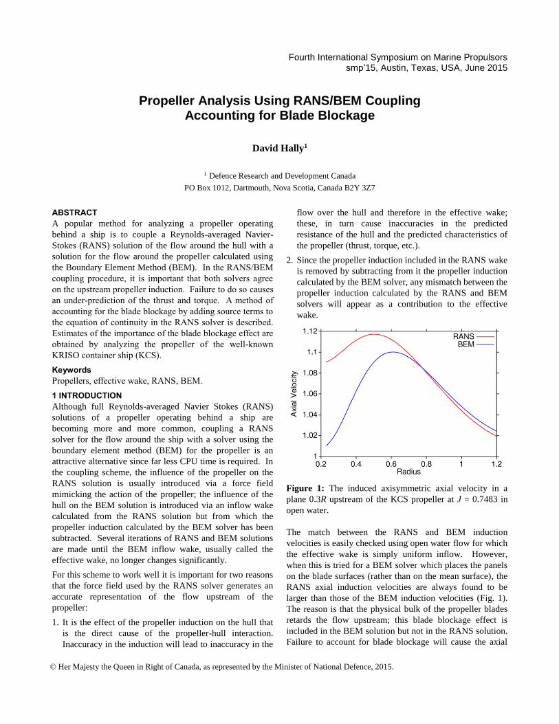
Figure 1: The induced axisymmetric axial velocity in a

plane 0.3R upstream of the KCS propeller at J = 0.7483 in

open water.

The match between the RANS and BEM induction

velocities is easily checked using open water flow for which

the effective wake is simply uniform inflow. However,

when this is tried for a BEM solver which places the panels

on the blade surfaces (rather than on the mean surface), the

RANS axial induction velocities are always found to be

larger than those of the BEM induction velocities (Fig. 1).

The reason is that the physical bulk of the propeller blades

retards the flow upstream; this blade blockage effect is

included in the BEM solution but not in the RANS solution.

Failure to account for blade blockage will cause the axial

© Her Majesty the Queen in Right of Canada, as represented by the Minister of National Defence, 2015.

velocity in the effective wake to be increased by the

discrepancy effectively increasing the advance coefficient,

J, and reducing the predicted thrust and torque.

Besides the numerical errors caused by the mismatch in

induction, the blade blockage has physical effects. Since

the induction is reduced, so is the thrust deduction. The

difference between the nominal and effective wakes will

also be somewhat smaller; since the effective wake is

normally accelerated relative to the nominal wake, the blade

blockage will tend to decrease the wake fraction, 1 − 𝑤.

For a fixed rotation rate, both effects lead to an increase of

speed at the self-propulsion point; if the speed is held

constant, both tend to decrease the rotation rate. Are these

changes significant?

Hally and Laurens (1998) attempted to account for the blade

blockage by calculating the flow within the blades in the

BEM solver and using the pressure difference across the

blade surface to adjust the force used in the RANS solver.

Rijpkema et al. (2013) removed the blade blockage from the

BEM induction by calculating it using only the dipole terms

in the BEM solution; since they use BEM based on the

Morino method (Morino and Kuo 1974), the blade blockage

is represented by the source terms; however, this approach

has the disadvantage that the induction is overestimated, so

the difference between the nominal and effective wakes will

also be overestimated. Therefore, while it reduces the

numerical errors by avoiding the mismatch in the induction,

it retains errors caused by the physical effects of an

overestimated induction in the RANS solution.

This paper describes a third method: the blade blockage is

included in the RANS solution by adding mass source terms

to the equation of motion. Because the blockage is

modelled in both RANS and BEM calculations, the

numerical errors caused by a mismatch in induction are

avoided and the physical effects of the blockage are taken

into account. It has been implemented using the open

source RANS solver OpenFOAM® and the BEM propeller

code PROCAL developed by Cooperative Research Ships.

PROCAL uses the Morino method (Morino and Kuo 1974)

to calculate the velocity potential of the disturbed flow and

has been validated extensively (Vaz and Bosschers 2006,

Bosschers et al. 2008).

The new method has been used to investigate the

importance of the blade blockage on the calculation of

propeller performance.

2 RANS EQUATIONS WITH MASS SOURCES

When the blade blockage is modelled using mass source

terms, the equations of motion to be solved by the RANS

solver are

𝜕𝑣𝑖

𝜕𝑥𝑖

= 𝑀, (1)

𝜕𝑣𝑖

𝜕𝑡+

𝜕(𝑣𝑖𝑣𝑗)

𝜕𝑥𝑗

=

−1

𝜌

𝜕𝑝

𝜕𝑥𝑖

+𝜕

𝜕𝑥𝑗

[𝜈𝑡 (𝜕𝑣𝑖

𝜕𝑥𝑗

+𝜕𝑣𝑗

𝜕𝑥𝑖

) + 𝛿𝑖𝑗

𝜕𝑣𝑘

𝜕𝑥𝑘

] + 𝐹𝑖 + 𝑀𝑣𝑖

(2)

with implicit summation over repeated indices. The

specific mass source density, 𝑀, and the force density, 𝐹𝑖,

are determined from the BEM solution from the mass flux

through each blade panel and the pressure on each blade

panel respectively. The term proportional to 𝑀 in the

momentum equation (Eq. 2) arises when one puts the

convective term in strong conservation form since the

divergence of the velocity is no longer uniformly zero. To

be completely consistent, one should add similar terms to

the transport equations in the turbulence model. However,

for the calculations described here, that was not done.

Adding these terms would cause small changes to the flow

downstream of the propeller; the change to the effective

wake would be negligible.

Although, as indicated in Eq. 2, it is possible to use

unsteady force and mass source fields in the RANS solver,

the computational effort increases significantly. Since the

main purpose for using the RANS/BEM coupling is to

reduce the computation time, in the method described here

the force and mass source fields are averaged in time. The

RANS solution is then steady.

The RANS solver used in the method must allow source

terms to be added to both the continuity equation and the

momentum equations.

2.1 Calculation of the force and mass source densities

The calculation of the force and mass source densities is

done in a cylindrical coordinate system, (𝑥, 𝑟, 𝜃), aligned

with the propeller axis. The force density at a point within

the volume swept out by the propeller is

𝑭 = ∑

𝑍𝑝�̂�

2𝜋𝜌𝑟|�̂� ∙ �̂�|𝑓,𝑏

(3)

where 𝑍 is the number of blades, 𝑝 is the pressure on the

blade as it passes through the point, �̂� is the normal to the

blade, 𝜌 is the fluid density and �̂� is a unit vector in the

direction of rotation. The sum represents the fact that at

each point one gets a contribution from both the face and

the back of each blade. The dot product in the denominator

is a geometric factor which accounts for the orientation of

the blade normal to the direction of averaging (�̂�).

Similarly, the specific mass source density is obtained from

the mass flux through the blades by the inflow:

𝑀 = ∑

−𝑍(𝑽 + 𝜔𝑟�̂�) ∙ �̂�

2𝜋𝑟|�̂� ∙ �̂�|𝑓,𝑏

= ∑−𝑍𝑽 ∙ �̂�

2𝜋𝑟|�̂� ∙ �̂�|𝑓,𝑏

+𝑍𝜔

2𝜋∑ sgn(�̂� ∙ �̂�)

𝑓,𝑏

= ∑−𝑍𝑽 ∙ �̂�

2𝜋𝑟|�̂� ∙ �̂�|𝑓,𝑏

(4)

Notice that the term in 𝜔 will vanish because the

contribution from the face of the blade will exactly cancel

the contribution from the back.

It is assumed that in the BEM solver the blades are covered

by a mesh of quadrilateral panels which rotate through

constant time steps. At each time step, the pressure at each

panel corner point is known. As it rotates from one time

step to the next, each panel sweeps out a hexahedral prism

in the cylindrical coordinate space. The integrals of 𝑭 and

𝑀 over the hexahedron are easily calculated by constructing

a trilinear interpolant between the values at the corner

points. One obtains the force and volume rate associated

with the hexahedron. Like the methods of force allocation

described by Hally and Laurens (1998) and Rijpkema et al.

(2013), each hexahedron is split into smaller hexahedra

until the force and mass rate from each can be assigned to a

cell in the RANS grid. The following algorithm is used:

1. Make a queue of all the hexahedra. The initial order of

the hexahedra is not important.

2. Assign a split level of zero to each hexahedron.

3. Set a maximum allowed split level.

4. For each hexahedron, find the cells in the RANS grid

which contain its corner points and store them with the

hexahedron.

5. Repeat until the queue is empty:

a. Remove the first hexahedron from the queue.

b. If any two neighbouring corner points lie in different

RANS cells that are not neighbours, then split the

hexahedron in the direction of the edge, set the split

level for each new hexahedron to the split level of the

original hexahedron, and add the two hexahedra to the

end of the queue. When the hexahedron is split, four

new corner points are created; the RANS cells

containing the corner points are found and stored with

the new hexahedra.

c. Otherwise, if all the corner points lie in the same

RANS cell, calculate the force and volume rate for the

hexahedron and assign them to that cell.

d. Otherwise, if the split level is the maximum allowed,

calculate the force and volume rate for the hexahedron

then, for each corner point, assign one eighth of the

force and volume rate to the RANS cell containing the

corner.

e. Otherwise, split the hexahedron along its longest edge,

set the split level for the two new hexahedra to one

more than the split level of the original hexahedron,

and add the two hexahedra to the end of the queue.

6. For each cell in the RANS grid, divide the assigned force

and volume rate by the volume of the cell to obtain a

force density and specific mass density for the cell.

Step 4.b ensures that all the cells in the RANS grid which

touch a hexahedron will be allocated a portion of its force

and volume rate. Without this step, when the hexahedra are

larger than the RANS cells (e.g. in the boundary layer of the

shaft) it would be possible to miss RANS cells resulting in

very uneven force and mass density fields.

Note, too, that the split level of a hexahedron is not

increased until the criterion in 4.b. is satisfied; therefore the

maximum split level is the number of times a hexahedron

can be split once all its corner points lie in neighbouring

cells in the RANS grid. A maximum split level of 3

provides a reasonable compromise between execution time

and accuracy of the force and mass density distributions.

To implement this algorithm efficiently, it is essential that

the search to find which cell in the RANS grid contains a

corner point can be performed quickly. For this purpose the

collection of RANS cells is first reduced to contain only

those cells which intersect the swept volume of the blades.

A hierarchy of bounding boxes for these cells is

constructed. Each member of the hierarchy contains a

range of cells, a bounding box for all the cells, and two

pointers to lower branch of the hierarchy covering the first

half of the range and the second half of the range. At the

lowest level of the hierarchy, the range consists of a single

cell. The cell containing a point is obtained by traversing

the hierarchy to find a collection of cells whose bounding

boxes contain the point (typically there will be only one or

two of them), then querying those cells to determine which

contains the point. The complexity of the search algorithm

is 𝑂(log 𝑁) where 𝑁 is the number of cells in the reduced

set of RANS cells.

The full allocation algorithm requires that the following

information be available from the RANS solver:

1. the number of cells in the RANS grid;

2. the volume of any cell;

3. a function to determine whether a point lies in a given

cell;

4. a function that indicates whether a given pair of cells are

neighbours; and

5. a bounding box for any cell (easily constructed from the

corner points of the cell).

Each of these is available in the OpenFOAM mesh data

structures.

2.2 Implementation in OpenFOAM

In the SIMPLE algorithm as implemented in OpenFOAM,

the linearized discretized momentum equations are written

in the form

𝑨𝑼 = 𝑯 − ∇𝑝 (5) Where 𝑼 represents the velocity at each cell, 𝑨 is a

diagonal matrix and 𝑯 includes all the off-diagonal terms

not dependent on the pressure. This equation is used to

obtain an expression for 𝑼,

𝑼 = 𝑨−1𝑯 − 𝑨−1∇𝑝, (6)

the divergence of which provides an equation for the

pressure, 𝑝:

𝛁 ∙ (𝑨−1∇𝑝) = 𝛁 ∙ (𝑨−1𝑯) − 𝑀 (7)

Therefore, in OpenFOAM, the source term 𝐹𝑖 + 𝑀𝑣𝑖 must

be added to the momentum equations and the source term

−𝑀 to the pressure equation.

To apply source terms in OpenFOAM one defines a class

which applies the sources to the appropriate equations.

Compiled code for the class is loaded at run-time. This

mechanism has been used to implement the algorithm

described in Sec. 2.1 and to apply the force and mass

densities to the momentum and pressure equations.

However, in OpenFOAM version 2.1 it is assumed that

there will be no sources for the pressure equation so an

additional modification is required to include them.

Unfortunately, OpenFOAM contains many different solvers

depending on the type of flow that is to be solved (steady,

incompressible, with free surface, etc.) and each must be

modified separately to include the mass density terms. To

date, we have only modified simpleFoam, the solver for

incompressible steady single-phase flows.

3 IMPLEMENTATION OF THE RANS/BEM COUPLING

The effective wake is the total wake in the propeller disk

(𝑥 = 0) with the propeller induction subtracted from it. At

iteration i of the RANS/BEM coupling, an approximation to

the effective wake is given by

𝒗eff𝑖 (𝑟, 𝜃) = 𝒗RANS

𝑖−1 (0, 𝑟, 𝜃)

− (𝒗BEM𝑖−1 (0, 𝑟, 𝜃) − 𝒗eff

𝑖−1(𝑟, 𝜃))

= 𝒗eff𝑖−1(𝑟, 𝜃) + ∆𝒗(0, 𝑟, 𝜃)

(8)

where 𝒗RANS is the total wake calculated by the RANS

solver, 𝒗BEM the total wake calculated by the BEM solver

and ∆𝒗 is their difference. The term in brackets is the

induced velocity calculated by the BEM solver since

𝒗eff𝑖−1(𝑟, 𝜃) is the wake in the propeller plane used as the

inflow to the BEM solver on the previous iteration.

Because of the presence of the propeller blades,

𝒗BEM𝑖−1 (𝑥, 𝑟, 𝜃) is only available at points upstream of the

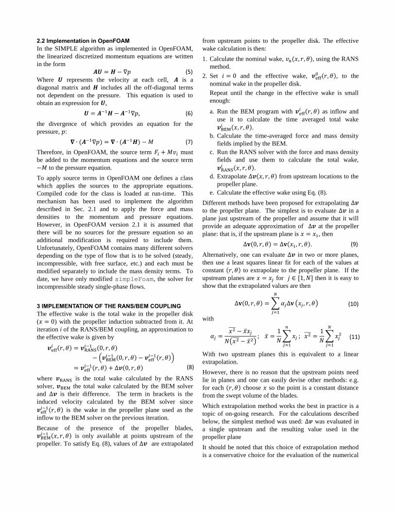
propeller. To satisfy Eq. (8), values of ∆𝒗 are extrapolated

from upstream points to the propeller disk. The effective

wake calculation is then:

1. Calculate the nominal wake, 𝑣n(𝑥, 𝑟, 𝜃), using the RANS

method.

2. Set 𝑖 = 0 and the effective wake, 𝒗eff0 (𝑟, 𝜃), to the

nominal wake in the propeller disk.

Repeat until the change in the effective wake is small

enough:

a. Run the BEM program with 𝒗eff𝑖 (𝑟, 𝜃) as inflow and

use it to calculate the time averaged total wake

𝒗BEM𝑖 (𝑥, 𝑟, 𝜃).

b. Calculate the time-averaged force and mass density

fields implied by the BEM.

c. Run the RANS solver with the force and mass density

fields and use them to calculate the total wake,

𝒗RANS𝑖 (𝑥, 𝑟, 𝜃).

d. Extrapolate ∆𝒗(𝑥, 𝑟, 𝜃) from upstream locations to the

propeller plane.

e. Calculate the effective wake using Eq. (8).

Different methods have been proposed for extrapolating ∆𝒗

to the propeller plane. The simplest is to evaluate ∆𝒗 in a

plane just upstream of the propeller and assume that it will

provide an adequate approximation of ∆𝒗 at the propeller

plane: that is, if the upstream plane is 𝑥 = 𝑥1, then

∆𝐯(0, 𝑟, 𝜃) = ∆𝐯(𝑥1, 𝑟, 𝜃). (9)

Alternatively, one can evaluate ∆𝒗 in two or more planes,

then use a least squares linear fit for each of the values at

constant (𝑟, 𝜃) to extrapolate to the propeller plane. If the

upstream planes are 𝑥 = 𝑥𝑗 for 𝑗 ∈ [1, 𝑁] then it is easy to

show that the extrapolated values are then

∆𝐯(0, 𝑟, 𝜃) = ∑ 𝛼𝑗∆𝐯

𝑁

𝑗=1

(𝑥𝑗 , 𝑟, 𝜃)

(10)

with

𝛼𝑗 =

𝑥2̅̅ ̅ − �̅�𝑥𝑗

𝑁(𝑥2̅̅ ̅ − �̅�2); �̅� =

1

𝑁∑ 𝑥𝑗

𝑛

𝑗=1

; 𝑥2̅̅ ̅ =1

𝑁∑ 𝑥𝑗

2

𝑁

𝑗=1

(11)

With two upstream planes this is equivalent to a linear

extrapolation.

However, there is no reason that the upstream points need

lie in planes and one can easily devise other methods: e.g.

for each (𝑟, 𝜃) choose 𝑥 so the point is a constant distance

from the swept volume of the blades.

Which extrapolation method works the best in practice is a

topic of on-going research. For the calculations described

below, the simplest method was used: ∆𝒗 was evaluated in

a single upstream and the resulting value used in the

propeller plane

It should be noted that this choice of extrapolation method

is a conservative choice for the evaluation of the numerical

errors associated with the mismatch of the RANS and BEM

induction. When blade blockage is ignored, the mismatch

increases as one approaches the propeller. Linear or least

squares extrapolation of ∆𝒗 to the propeller plane will then

tend to increase the mismatch causing larger errors.

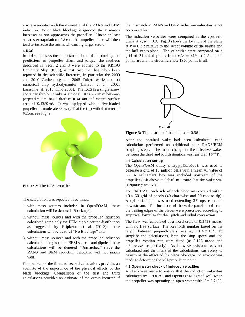
4 KCS

In order to assess the importance of the blade blockage on

predictions of propeller thrust and torque, the methods

described in Secs. 2 and 3 were applied to the KRISO

Container Ship (KCS), a test case that has often been

reported in the scientific literature, in particular the 2000

and 2010 Gothenburg and 2005 Tokyo workshops on

numerical ship hydrodynamics (Larrson et al., 2002,

Larsson et al. 2013, Hino 2005). The KCS is a single screw

container ship built only as a model. It is 7.2785m between

perpendiculars, has a draft of 0.3418m and wetted surface

area of 9.4389 m2. It was equipped with a five-bladed

propeller of moderate skew (24º at the tip) with diameter of

0.25m: see Fig. 2.

Figure 2: The KCS propeller.

The calculation was repeated three times:

1. with mass sources included in OpenFOAM; these

calculation will be denoted “Blockage”;

2. without mass sources and with the propeller induction

calculated using only the BEM dipole source distribution

as suggested by Rijpkema et al. (2013); these

calculations will be denoted “No Blockage” and

3. without mass sources and with the propeller induction

calculated using both the BEM sources and dipoles; these

calculations will be denoted “Unmatched” since the

RANS and BEM induction velocities will not match

well.

Comparison of the first and second calculations provides an

estimate of the importance of the physical effects of the

blade blockage. Comparison of the first and third

calculations provides an estimate of the errors incurred if

the mismatch in RANS and BEM induction velocities is not

accounted for.

The induction velocities were compared at the upstream

plane at 𝑥/𝑅 = 0.3. Fig. 3 shows the location of the plane

at 𝑥 = 0.3𝑅 relative to the swept volume of the blades and

the hull centreplane. The velocities were compared on a

grid of 21 radial points from 𝑟 𝑅⁄ = 0.19 to 1.2 and 90

points around the circumference: 1890 points in all.

Figure 3: The location of the plane 𝑥 = 0.3𝑅.

After the nominal wake had been calculated, each

calculation performed an additional four RANS/BEM

coupling steps. The mean change in the effective wakes

between the third and fourth iteration was less than 10−4𝑉.

4.1 Calculation set-up

The OpenFOAM utility snappyHexMesh was used to

generate a grid of 10 million cells with a mean 𝑦+ value of

66. A refinement box was included upstream of the

propeller disk above the shaft to ensure that the wake was

adequately resolved.

For PROCAL, each side of each blade was covered with a

40 × 30 grid of panels (40 chordwise and 30 root to tip).

A cylindrical hub was used extending 3𝑅 upstream and

downstream. The locations of the wake panels shed from

the trailing edges of the blades were prescribed according to

empirical formulae for their pitch and radial contraction

The flow was calculated at a fixed draft of 0.3418 metres

with no free surface. The Reynolds number based on the

length between perpendiculars was 𝑅𝑒 = 1.4 × 107. To

simplify the calculations, both the ship speed and the

propeller rotation rate were fixed (at 2.196 m/sec and

9.5 revs/sec respectively). As the wave resistance was not

calculated and the intent of the calculations was solely to

determine the effect of the blade blockage, no attempt was

made to determine the self-propulsion point.

4.2 Open water check of induced velocities

A check was made to ensure that the induction velocities

calculated by PROCAL and OpenFOAM agreed well when

the propeller was operating in open water with J = 0.7483,

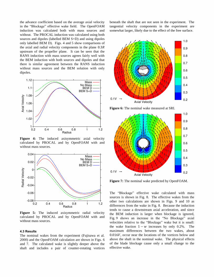
the advance coefficient based on the average axial velocity

in the “Blockage” effective wake field. The OpenFOAM

induction was calculated both with mass sources and

without. The PROCAL induction was calculated using both

sources and dipoles (labelled BEM S+D) and using dipoles

only labelled BEM D). Figs. 4 and 5 show comparisons of

the axial and radial velocity components in the plane 0.3𝑅

upstream of the propeller plane. It can be seen that the

RANS induction with mass sources agrees fairly well with

the BEM induction with both sources and dipoles and that

there is similar agreement between the RANS induction

without mass sources and the BEM solution with only

dipoles.

Figure 4: The induced axisymmetric axial velocity

calculated by PROCAL and by OpenFOAM with and

without mass sources.

Figure 5: The induced axisymmetric radial velocity

calculated by PROCAL and by OpenFOAM with and

without mass sources.

4.3 Results

The nominal wakes from the experiment (Fujisawa et al.

2000) and the OpenFOAM calculation are shown in Figs. 6

and 7. The calculated wake is slightly deeper above the

shaft and includes a pair of counter-rotating vortices

beneath the shaft that are not seen in the experiment. The

tangential velocity components in the experiment are

somewhat larger, likely due to the effect of the free surface.

Figure 6: The nominal wake measured at SRI.

Figure 7: The nominal wake predicted by OpenFOAM.

The “Blockage” effective wake calculated with mass

sources is shown in Fig. 8. The effective wakes from the

other two calculations are shown in Figs. 9 and 10 as

differences from the wake in Fig. 8. Because the induction

tends to cause a downstream axial acceleration, and since

the BEM induction is larger when blockage is ignored,

Fig. 9 shows an increase in the “No Blockage” axial

velocities relative to the “Blockage” wake but it is small:

the wake fraction 1 − 𝑤 increases by only 0.2%. The

maximum differences between the two wakes, about

0.016𝑉, occur near the locations of the vortices below and

above the shaft in the nominal wake. The physical effects

of the blade blockage cause only a small change to the

effective wake.

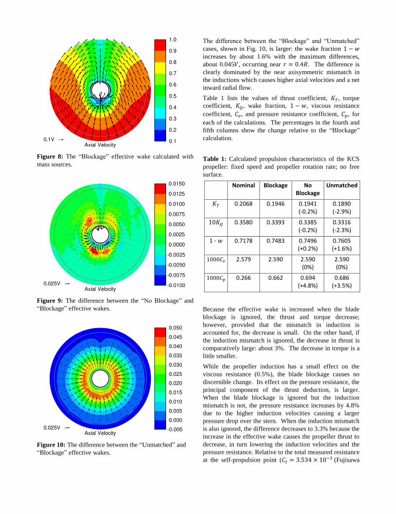
Figure 8: The “Blockage” effective wake calculated with

mass sources.

Figure 9: The difference between the “No Blockage” and

“Blockage” effective wakes.

Figure 10: The difference between the “Unmatched” and

“Blockage” effective wakes.

The difference between the “Blockage” and “Unmatched”

cases, shown in Fig. 10, is larger: the wake fraction 1 − 𝑤

increases by about 1.6% with the maximum differences,

about 0.045𝑉, occurring near 𝑟 = 0.4𝑅. The difference is

clearly dominated by the near axisymmetric mismatch in

the inductions which causes higher axial velocities and a net

inward radial flow.

Table 1 lists the values of thrust coefficient, 𝐾𝑇, torque

coefficient, 𝐾𝑄, wake fraction, 1 − 𝑤, viscous resistance

coefficient, 𝐶𝑣, and pressure resistance coefficient, 𝐶𝑝, for

each of the calculations. The percentages in the fourth and

fifth columns show the change relative to the “Blockage”

calculation.

Table 1: Calculated propulsion characteristics of the KCS

propeller: fixed speed and propeller rotation rate; no free

surface.

Nominal Blockage No Blockage

Unmatched

𝐾𝑇 0.2068 0.1946 0.1941 (-0.2%)

0.1890 (-2.9%)

10𝐾𝑄 0.3580 0.3393 0.3385 (-0.2%)

0.3316 (-2.3%)

1 - 𝑤 0.7178 0.7483 0.7496 (+0.2%)

0.7605 (+1.6%)

1000𝐶𝑣 2.579 2.590 2.590 (0%)

2.590 (0%)

1000𝐶𝑝 0.266 0.662 0.694 (+4.8%)

0.686 (+3.5%)

Because the effective wake is increased when the blade

blockage is ignored, the thrust and torque decrease;

however, provided that the mismatch in induction is

accounted for, the decrease is small. On the other hand, if

the induction mismatch is ignored, the decrease in thrust is

comparatively large: about 3%. The decrease in torque is a

little smaller.

While the propeller induction has a small effect on the

viscous resistance (0.5%), the blade blockage causes no

discernible change. Its effect on the pressure resistance, the

principal component of the thrust deduction, is larger.

When the blade blockage is ignored but the induction

mismatch is not, the pressure resistance increases by 4.8%

due to the higher induction velocities causing a larger

pressure drop over the stern. When the induction mismatch

is also ignored, the difference decreases to 3.3% because the

increase in the effective wake causes the propeller thrust to

decrease, in turn lowering the induction velocities and the

pressure resistance. Relative to the total measured resistance

at the self-propulsion point (𝐶𝑡 = 3.534 × 10−3 (Fujisawa

et al. 2000)) these represent changes of about 0.9% and

0.7% respectively; that is, failure to account for the blade

blockage causes a change in the total resistance of a little

less than 1% (it will be smaller at full scale).

If blade blockage is not accounted for, the increase in

pressure resistance and the decrease in thrust combine to

require an increase of thrust at the self-propulsion point: if

the mismatch in induction is taken into account, the

required increase is about 1.4%; if the mismatch in

induction is ignored it is about 4%.

6 CONCLUSIONS Failure to account for blade blockage when matching the

RANS and BEM induction will lead to errors in ship

powering predictions. The calculations described here

suggest that, for typical single screw vessels, the physical

effect of the blockage is to increase the thrust required at the

self-propulsion point by the order of 1%. Most of this is

due to an increase in the thrust deduction caused by the

slower velocities upstream of the propeller caused by the

blockage; a smaller part is caused by a small increase of the

axial velocities in the effective wake causing the propeller

to deliver less thrust.

When RANS/BEM coupling is used, the blade blockage

also causes a mismatch in the induction velocities predicted

by the RANS and BEM solvers since the blockage will be

included in the BEM solution but not in the RANS solution.

If this mismatch is not accounted for, the under-prediction

of the required thrust at the self-propulsion point will be of

the order of 4%. If linear or least squares extrapolation is

used for ∆𝑣, this under-prediction will be larger (likely

about 5%).

The mismatch in the RANS and BEM inductions can be

corrected either by introducing the blockage into the RANS

solution as described in Sec. 2 or by removing it from the

BEM solution as in the method of Rijpkema et al. The

former method has the advantage that the physical effects of

the blockage are also included in the solution while they are

ignored by the latter method. However, since the physical

effects are small enough that they are very likely within the

overall accuracy of the method, either method should give

acceptable results.

REFERENCES

Bosschers, J., Vaz, G., Starke A.R., and van Wijngaarden, E.

(2008). “Computational analysis of propeller sheet

cavitation and propeller-ship interaction,” Proc. of

RINA MARINE CFD Conference CFD2008,

Southampton, UK.

Hally, D., and Laurens J.-M. (1998). “Numerical Simulation

of Hull-propeller Interaction Using Force Fields with

Navier-Stokes Computations,” Ship Technology

Research, 45(1), 28-36.

Hino, T. (2005). Proc. of CFD Workshop Tokyo 2005,

Tokyo, Japan.

Rijpkema, D., Starke, B., and Bosschers, J. (2013).

“Numerical simulation of propeller-hill interaction and

determination of the effective wake field using a hybrid

RANS-BEM approach,” Proc. 3rd International

Symposium on Marine Propulsors, Launceston,

Tasmania, Australia.

Fujisawa, J., Ukon, Y., Kume, K., and Takeshi, H. (2000),

“Local Velocity Field Measurements Around the KCS

Model (SRI M.S. No. 631) in the SRI 400m Towing

Tank,” SPD Report No. 00-003-2, Ship Research

Institute, Ministry of Transport, Japan.

Larsson, L., Stern, F. and Bertram, V. (eds.), (2002).

Gothenburg 2000, A Workshop on Numerical Ship

Hydrodynamics, Chalmers University of Technology.

Larsson, L., Stern, F. and Visonneau, M. (eds.), (2013).

Numerical Ship Hydrodynamics: An assessment of the

Gothenburg 2010 workshop, Springer.

Morino, L. and Kuo, C.C. (1974). “Subsonic Potential

Aerodynamics for complex configurations,” AIAA

Journal 12(2), 191-197.

Vaz, G. and Bosschers, J. (2006). “Modelling of three-

dimensional sheet cavitation on marine propellers using

a boundary element method,” Proc. of 6th Inter. Symp.

On Cavitation CAV2006, Wageningen, The Netherlands.

DISCUSSION

Question from Dmitriy Ponkratov

How were the induced velocities calculated?

Author’s Closure

As described in Section 3, the induced velocity is obtained

from the BEM solution by subtracting the current estimate

of the effective wake (the inflow into the propeller) from

the BEM velocity field in the propeller plane (𝑥 = 0). At

iteration i this can be written as:

𝐯ind𝑖 (0, 𝑟, 𝜃) = 𝐯BEM

𝑖 (0, 𝑟, 𝜃) − 𝐯eff𝑖 (𝑟, 𝜃).

Note that the induced velocities are only needed in the

propeller plane but, to calculate them, it is necessary to

extrapolate the values of 𝐯BEM𝑖 from values upstream of the

propeller. The extrapolation procedure is also described in

Section 3.

Question from Johan Bosschers

Thank you for your presentation. Does the inclusion of the

mass terms in the RANS solver have an influence on the

iterative convergence?

Author’s Closure

Not of any significance. Figure 11 shows the RMS

difference in effective wake axial velocity between

iterations for each of the three cases that we computed

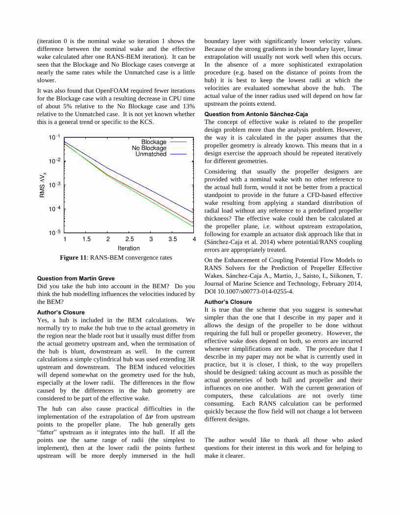
(iteration 0 is the nominal wake so iteration 1 shows the

difference between the nominal wake and the effective

wake calculated after one RANS-BEM iteration). It can be

seen that the Blockage and No Blockage cases converge at

nearly the same rates while the Unmatched case is a little

slower.

It was also found that OpenFOAM required fewer iterations

for the Blockage case with a resulting decrease in CPU time

of about 5% relative to the No Blockage case and 13%

relative to the Unmatched case. It is not yet known whether

this is a general trend or specific to the KCS.

Figure 11: RANS-BEM convergence rates

Question from Martin Greve

Did you take the hub into account in the BEM? Do you

think the hub modelling influences the velocities induced by

the BEM?

Author’s Closure

Yes, a hub is included in the BEM calculations. We

normally try to make the hub true to the actual geometry in

the region near the blade root but it usually must differ from

the actual geometry upstream and, when the termination of

the hub is blunt, downstream as well. In the current

calculations a simple cylindrical hub was used extending 3R

upstream and downstream. The BEM induced velocities

will depend somewhat on the geometry used for the hub,

especially at the lower radii. The differences in the flow

caused by the differences in the hub geometry are

considered to be part of the effective wake.

The hub can also cause practical difficulties in the

implementation of the extrapolation of ∆𝒗 from upstream

points to the propeller plane. The hub generally gets

“fatter” upstream as it integrates into the hull. If all the

points use the same range of radii (the simplest to

implement), then at the lower radii the points furthest

upstream will be more deeply immersed in the hull

boundary layer with significantly lower velocity values.

Because of the strong gradients in the boundary layer, linear

extrapolation will usually not work well when this occurs.

In the absence of a more sophisticated extrapolation

procedure (e.g. based on the distance of points from the

hub) it is best to keep the lowest radii at which the

velocities are evaluated somewhat above the hub. The

actual value of the inner radius used will depend on how far

upstream the points extend.

Question from Antonio Sánchez-Caja

The concept of effective wake is related to the propeller

design problem more than the analysis problem. However,

the way it is calculated in the paper assumes that the

propeller geometry is already known. This means that in a

design exercise the approach should be repeated iteratively

for different geometries.

Considering that usually the propeller designers are

provided with a nominal wake with no other reference to

the actual hull form, would it not be better from a practical

standpoint to provide in the future a CFD-based effective

wake resulting from applying a standard distribution of

radial load without any reference to a predefined propeller

thickness? The effective wake could then be calculated at

the propeller plane, i.e. without upstream extrapolation,

following for example an actuator disk approach like that in

(Sánchez-Caja et al. 2014) where potential/RANS coupling

errors are appropriately treated.

On the Enhancement of Coupling Potential Flow Models to

RANS Solvers for the Prediction of Propeller Effective

Wakes. Sánchez-Caja A., Martio, J., Saisto, I., Siikonen, T.

Journal of Marine Science and Technology, February 2014,

DOI 10.1007/s00773-014-0255-4.

Author’s Closure

It is true that the scheme that you suggest is somewhat

simpler than the one that I describe in my paper and it

allows the design of the propeller to be done without

requiring the full hull or propeller geometry. However, the

effective wake does depend on both, so errors are incurred

whenever simplifications are made. The procedure that I

describe in my paper may not be what is currently used in

practice, but it is closer, I think, to the way propellers

should be designed: taking account as much as possible the

actual geometries of both hull and propeller and their

influences on one another. With the current generation of

computers, these calculations are not overly time

consuming. Each RANS calculation can be performed

quickly because the flow field will not change a lot between

different designs.

The author would like to thank all those who asked

questions for their interest in this work and for helping to

make it clearer.