Embed Size (px)
Citation preview
Properties of Cherednik algebras
and graded Hecke algebras
by
Katrin Eva Gehles
A thesis submitted to the
Faculty of Information and Mathematical Sciences
at the University of Glasgow
for the degree of
Doctor of Philosophy
April 2006
c© K E Gehles 2006

i
For my family
Acknowledgements
Above all I am grateful to my supervisors Ken A. Brown and Iain Gordon for their con-
tinuous assistance and encouragement. Their guidance and advice has been invaluable.
My special thanks go to my family for their love and support, which kept me grounded.
I also wish to thank all the postgraduate students and friends I met along the way, most
notably Mo, without whom my stay in Glasgow could not have been as enjoyable.
Finally, I thank EPSRC and the University of Glasgow for their financial support
throughout my studies.
ii
Summary
The objects of investigation in this thesis are four distinct but related types of algebras,
namely the Cherednik algebras and graded Hecke algebras of the title. There are two
aspects which connect these four kinds of algebras. Firstly, they are all non-commutative
deformations of some skew group algebras. Secondly, symplectic reflection algebras ap-
pear in all cases as certain specialisations or degenerations of the algebras in question. Our
interest lies in examining ring-theoretic properties of these algebras with a view towards
applications to geometric questions.
In Chapter 1 we present some basic definitions and background material, which we will
refer to in the remainder of this document.
Chapter 2 is dedicated to introducing the three types of algebras that are subsumed
under the name Cherednik algebras. These are the double affine Hecke algebra, the trigono-
metric double affine Hecke algebra and the rational Cherednik algebra, see [Che04] for an
overview. We begin a ring-theoretic study of the double affine Hecke algebra and the
trigonometric double affine Hecke algebra. In particular, we provide at least partial an-
swers to the questions whether these rings are noetherian and prime. We also investigate
their global dimensions. Cherednik algebras all display a dichotomy in their behaviour
depending on the specialisation of certain parameters. The parameter specialisations for
which the Cherednik algebras are finitely generated over their centres and thus PI algebras
are of particular interest to us, because in these cases connections to algebraic geometry
come to the forefront. Therefore, we investigate the ring-theoretic properties of the PI
Cherednik algebras in more detail and provide faithful representations for these algebras.
Our description of these representations is very explicit and makes statements by [Obl04]
precise. From these representations we obtain embeddings of the PI Cherednik algebras
iii
iv
into skew group algebras.
The second aim of our study of Cherednik algebras is to understand the connections
between the PI cases of these three kinds of algebras. In Chapter 3 we concentrate on the
Cherednik algebras attached to the root system of type A1. In this example we are able
to set up a framework of relations between the PI Cherednik algebras. The processes of
degeneration and completion, which make up this framework, are described in sufficient
detail to enable us to transfer across geometric information from the PI rational Cherednik
algebra to the PI double affine Hecke algebra. Following Lusztig’s work on affine Hecke
algebras in [Lus89] we first consider the process of degeneration: using certain filtrations
of the Cherednik algebras and the corresponding associated graded algebras one can pass
from the double affine Hecke algebra via the trigonometric double affine Hecke algebra to
the rational Cherednik algebra. Secondly, again extending the work in [Lus89], we show
that the PI Cherednik algebras of type A1 are isomorphic after completing at suitable
ideals. These isomorphisms turn out to be isomorphisms between the completions of the
skew group algebras into which we embedded the PI Cherednik algebras in the previous
chapter. Chapter 3 concludes with an explanation of how this framework of degeneration
and completion can be used to answer geometric questions about these PI algebras.
Finally, Chapter 4 contains our work on graded Hecke algebras, which were defined
by [Dri86] and [RS03]. We show that, similarly to the Cherednik algebras, graded Hecke
algebras are finitely generated over their centres precisely when certain parameters are
specialised to zero. Graded Hecke algebras can be viewed as generalisations of symplectic
reflection algebras and our result generalises work by Etingof and Ginzburg for symplectic
reflection algebras, [EG02]. After deriving some of the basic properties of graded Hecke
algebras we introduce the theory of PBW deformations to motivate the definition of these
algebras. We then proceed by examining the spherical subalgebra of a graded Hecke
algebra, which plays a crucial role in proving our main theorem. In our treatment we
follow the strategy used in [EG02] to study symplectic reflection algebras. The concept
of a Poisson bracket and the theory of orbit varieties feature in the proofs of further
preliminary results. The understanding we gained from considering graded Hecke algebras
as PBW deformations then allows us to deduce the main theorem.
Statement
This thesis is submitted in accordance with regulations for the degree of Doctor of Philos-
ophy in the University of Glasgow. No part of this thesis has previously been submitted
by me for a degree at this or any other university.
Chapter 1 covers definitions and basic results. Sections 3.2, 3.3, 4.3 - 4.5 consist of
the author’s original work. Further original work by the author is contained in Chapter 2
unless referenced otherwise.
v
Contents
Acknowledgements ii
Summary iii
Statement v
Introduction 1
1 Notation and preliminaries 12
1.1 Localisations of non-commutative rings . . . . . . . . . . . . . . . . . . . . . 12
1.2 Associated graded algebras . . . . . . . . . . . . . . . . . . . . . . . . . . . 14
1.3 PI algebras . . . . . . . . . . . . . . . . . . . . . . . . . . . . . . . . . . . . 15
1.4 Smoothness and Azumaya algebras . . . . . . . . . . . . . . . . . . . . . . . 17
1.5 Completions . . . . . . . . . . . . . . . . . . . . . . . . . . . . . . . . . . . . 18
1.6 Skew group algebras and invariant rings . . . . . . . . . . . . . . . . . . . . 19
2 Cherednik algebras 23
2.1 The double affine Hecke algebra . . . . . . . . . . . . . . . . . . . . . . . . . 24
2.1.1 Definition and first properties . . . . . . . . . . . . . . . . . . . . . . 24
2.1.2 The specialisation q = 1 . . . . . . . . . . . . . . . . . . . . . . . . . 33
2.2 The trigonometric double affine Hecke algebra . . . . . . . . . . . . . . . . . 40
2.2.1 Definition and first properties . . . . . . . . . . . . . . . . . . . . . . 40
2.2.2 The specialisation q = 0 . . . . . . . . . . . . . . . . . . . . . . . . . 52
2.3 The rational Cherednik algebra . . . . . . . . . . . . . . . . . . . . . . . . . 57
2.3.1 Definition and first properties . . . . . . . . . . . . . . . . . . . . . . 57
2.3.2 The specialisation q = 0 . . . . . . . . . . . . . . . . . . . . . . . . . 59
vi
CONTENTS vii
3 Equivalences of PI Cherednik algebras of type A1 63
3.1 The root system of type A1 . . . . . . . . . . . . . . . . . . . . . . . . . . . 63
3.1.1 The DAHA of type A1 . . . . . . . . . . . . . . . . . . . . . . . . . . 64
3.1.2 The trigonometric DAHA of type A1 . . . . . . . . . . . . . . . . . . 65
3.1.3 The RCA of type A1 . . . . . . . . . . . . . . . . . . . . . . . . . . . 66
3.2 Degenerations for type A1 . . . . . . . . . . . . . . . . . . . . . . . . . . . . 67
3.2.1 From the DAHA to the trigonometric DAHA . . . . . . . . . . . . . 67
3.2.2 From the trigonometric DAHA to the RCA . . . . . . . . . . . . . . 70
3.3 Completions for type A1 . . . . . . . . . . . . . . . . . . . . . . . . . . . . . 73
3.3.1 From the RCA to the trigonometric DAHA - at ideals corresponding
to the origin . . . . . . . . . . . . . . . . . . . . . . . . . . . . . . . 73
3.3.2 From the RCA to the trigonometric DAHA - at arbitrary maximal
ideals . . . . . . . . . . . . . . . . . . . . . . . . . . . . . . . . . . . 78
3.3.3 From the trigonometric DAHA to the DAHA - at ideals correspond-
ing to the origin . . . . . . . . . . . . . . . . . . . . . . . . . . . . . 82
3.3.4 From the trigonometric DAHA to the DAHA - at arbitrary maximal
ideals . . . . . . . . . . . . . . . . . . . . . . . . . . . . . . . . . . . 87
3.3.5 Geometric application . . . . . . . . . . . . . . . . . . . . . . . . . . 89
4 Graded Hecke algebras 93
4.1 Definition and first properties . . . . . . . . . . . . . . . . . . . . . . . . . . 93
4.2 PBW deformation . . . . . . . . . . . . . . . . . . . . . . . . . . . . . . . . 98
4.3 The spherical subalgebra . . . . . . . . . . . . . . . . . . . . . . . . . . . . . 109
4.4 Preliminary results . . . . . . . . . . . . . . . . . . . . . . . . . . . . . . . . 113
4.5 Proof of the main theorem . . . . . . . . . . . . . . . . . . . . . . . . . . . . 120
A Embeddings for PI Cherednik algebras of type A1 128
References 130
Introduction
Our research into the properties of Cherednik algebras and graded Hecke algebras was
inspired by results of first Etingof and Ginzburg in [EG02], then Gordon in [Gor03a], and
finally Oblomkov in [Obl04]. In these papers the representation theory of non-commutative
algebras is employed to tackle questions in algebraic geometry.
Symplectic reflection algebras
Traditionally, if G is a finite group acting on a smooth complex affine algebraic variety
X, then the orbit variety X/G can be studied via its coordinate ring C[X]G, the ring
of G-invariant regular functions on X. This study is part of geometric invariant theory.
One of the natural questions to ask is whether the variety X/G is smooth. When X is
a vector space and G acts linearly, the Chevalley-Shephard-Todd theorem implies that
X/G is smooth if and only if G is generated by complex reflections in its action on X.
If the variety X/G is singular, a possible next step is to find a smooth deformation of
the singularities. Recently, for example in [EG02], researchers have investigated the skew
group algebra C[X] ∗ G in order to study the G-equivariant geometry of X. Here C[X]
denotes the coordinate ring of X. The centre of C[X] ∗G is precisely the ring C[X]G. In
the case of a symplectic vector space V over C and G ⊆ GL(V ) a group that preserves the
symplectic form on V , Etingof and Ginzburg study non-commutative deformations of the
algebra C[V ] ∗G to great effect in [EG02]. They call the deformation algebras that occur
symplectic reflection algebras (SRA). In some cases their techniques indeed lead to the
discovery of smooth deformations of the singular symplectic varieties V/G. This work is
extended in [Gor03a] and produces an almost complete classification of the cases in which
a smooth deformation exists. There has also been progress on making the relationship
between the deformations and desingularisations of V/G precise, see for example [GS04].
1
CONTENTS 2
The algebras that we will explore in the following all demonstrate similar behaviour to
SRAs. In fact, Cherednik algebras and graded Hecke algebras are all directly related to
SRAs. Some of these algebras are generalisations or special cases of SRAs, whereas others
can be degenerated to a particular kind of SRA. Therefore we will expand a little on SRAs
before we examine the actual subjects of this thesis.
An SRA, say H, is a filtered algebra and is defined in such a way that grH ∼= C[V ]∗G,
where grH denotes the associated graded algebra of H. This fact is called the PBW
property of SRAs. SRAs depend on some deformation parameters and the PBW result
ensures that the algebras do not collapse for any specialisations of these parameters. The
characteristics of SRAs differ vastly depending on the specialisations of the deformation
parameters, one of which we denote by q. In particular, if q = 0 the SRA has a large centre
and the algebra is finitely generated over its centre. It is an old result that an algebra
which is finitely generated over its centre satisfies a polynomial identity. Therefore we
call this specialisation the PI case. When the parameter q is specialised to other values,
however, the centres of the SRAs are trivial. Thus it is the PI case in which questions
about the geometric structure of the variety corresponding to the centre of an SRA arise.
See [Bro02] for a survey of these results.
A key result in [EG02] - with a view to non-commutative geometry - is that the centre of
a PI SRA is a deformation of the coordinate ring of the variety V/G. The results in [EG02]
and [Gor03a] use representation theory to determine whether or not this deformation is
smooth. Firstly, if an SRA H is finitely generated over its centre, it can be shown, using
a generalised version of Schur’s lemma, that all simple H-modules are finite dimensional.
Secondly, there exists an upper bound for the dimensions of the simple H-modules and
the maximal dimension of a simple H-module is called the PI degree of H. Etingof and
Ginzburg showed in [EG02] that this number equals |G|, the order of the group. Finally,
if there exists a simple H-module of dimension less than |G|, then the algebra H is not
Azumaya. In the case of a PI SRA it is shown in [EG02] that the algebra H is Azumaya
if and only if the variety corresponding to its centre is smooth.
We will see that the Cherednik algebras and graded Hecke algebras are not only also
non-commutative deformations of skew group algebras, but they display the same di-
chotomy of behaviour for distinct specialisations of the deformation parameters as the
SRAs. Moreover, PBW results, analogous to the one for SRAs, exist in all our cases.
CONTENTS 3
More generally, the four types of algebras under investigation in this thesis are all
interesting examples of non-commutative affine C-algebras. They are interesting objects
to study in the area of non-commutative algebraic geometry, since they provide examples
of algebras which are finitely generated over their centres. Thus for these algebras there is
a strong connection between the geometry of the varieties associated to their centres and
the structure of the algebra itself and its representation theory. In addition, the various
Cherednik algebras and graded Hecke algebras have been crucial in proving results in other
areas of mathematics. In the following we will briefly mention some of these successes and
challenges involving Cherednik algebras and graded Hecke algebras.
Cherednik algebras
Let us specify which three algebras we subsume under the expression Cherednik algebras
and illustrate their interconnections. Suppose W is a finite Weyl group acting on its
reflection representation V over C and denote the dual space by V ∗. Then V ∗ contains
the root system R spanned by the simple roots α1, . . . , αn. Let β1, . . . , βn denote the
fundamental weights. In this situation we obtain a linear action of W on C[V ], the
algebra of polynomial functions on V . Hence C[V ] = C[x1, . . . , xn], where xi := xαi and
xα =∑n
i=1 λixi whenever α =∑n
i=1 λiαi. For w ∈W the action is given by wxα = xw(α).
Alternatively, one can begin by setting xi := xβiand then proceed in the same way.
Similarly, a multiplicative action on C[V ±1] := C[X±11 , . . . , X±1
n ] can be defined if we let
Xα =∏ni=1X
λii whenever α =
∑ni=1 λiαi. The actions of W on C[V ∗] and C[(V ∗)±1] are
given analogously.
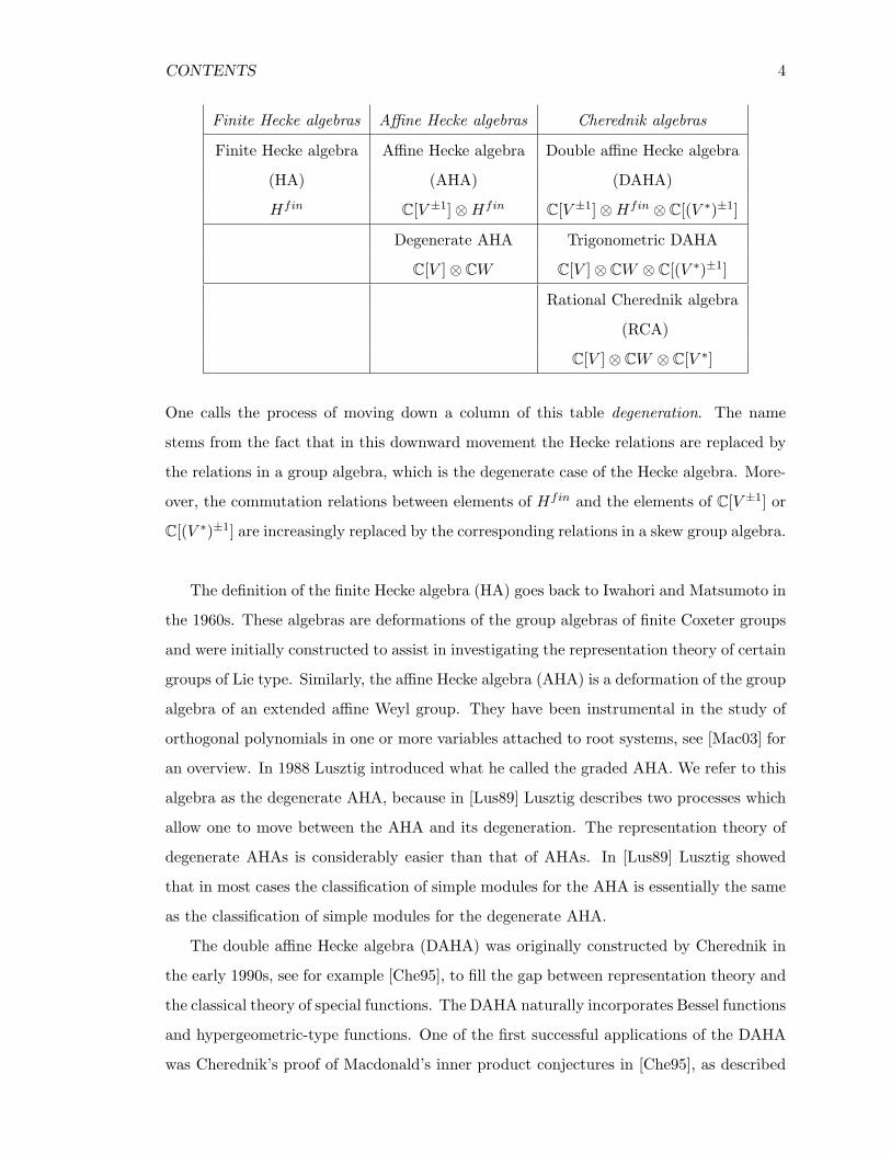
Over the last decades various Hecke-type algebras associated to W have been con-
structed, including the algebras we refer to as Cherednik algebras. These algebras can
be arranged in the following table, see [Rou05], which describes their structure as vector
spaces. The algebras in the right column of the table are the ones that we call Cherednik
algebras.
CONTENTS 4
Finite Hecke algebras Affine Hecke algebras Cherednik algebras
Finite Hecke algebra Affine Hecke algebra Double affine Hecke algebra
(HA) (AHA) (DAHA)
Hfin C[V ±1]⊗Hfin C[V ±1]⊗Hfin ⊗ C[(V ∗)±1]
Degenerate AHA Trigonometric DAHA
C[V ]⊗ CW C[V ]⊗ CW ⊗ C[(V ∗)±1]
Rational Cherednik algebra
(RCA)
C[V ]⊗ CW ⊗ C[V ∗]
One calls the process of moving down a column of this table degeneration. The name
stems from the fact that in this downward movement the Hecke relations are replaced by
the relations in a group algebra, which is the degenerate case of the Hecke algebra. More-
over, the commutation relations between elements of Hfin and the elements of C[V ±1] or
C[(V ∗)±1] are increasingly replaced by the corresponding relations in a skew group algebra.
The definition of the finite Hecke algebra (HA) goes back to Iwahori and Matsumoto in
the 1960s. These algebras are deformations of the group algebras of finite Coxeter groups
and were initially constructed to assist in investigating the representation theory of certain
groups of Lie type. Similarly, the affine Hecke algebra (AHA) is a deformation of the group
algebra of an extended affine Weyl group. They have been instrumental in the study of
orthogonal polynomials in one or more variables attached to root systems, see [Mac03] for
an overview. In 1988 Lusztig introduced what he called the graded AHA. We refer to this
algebra as the degenerate AHA, because in [Lus89] Lusztig describes two processes which
allow one to move between the AHA and its degeneration. The representation theory of
degenerate AHAs is considerably easier than that of AHAs. In [Lus89] Lusztig showed
that in most cases the classification of simple modules for the AHA is essentially the same
as the classification of simple modules for the degenerate AHA.
The double affine Hecke algebra (DAHA) was originally constructed by Cherednik in
the early 1990s, see for example [Che95], to fill the gap between representation theory and
the classical theory of special functions. The DAHA naturally incorporates Bessel functions
and hypergeometric-type functions. One of the first successful applications of the DAHA
was Cherednik’s proof of Macdonald’s inner product conjectures in [Che95], as described
CONTENTS 5
in the survey by Kirillov, [Kir97]. In addition to combinatorics, connections and potential
applications have been found to Lie algebras, Verlinde algebras and Kac-Moody algebras
for example, see [Che05, Introduction] for an overview. Cherednik attaches particular
importance to the example of the DAHA for the symmetric group in two letters, that is for
the root system of type A1. He believes that the DAHA of type A1 is the natural successor
of the Lie algebra sl(2), a major player in representation theory, see [Che05, Sections 0.2.1
and 0.3.2].
The trigonometric DAHA is a degeneration of the DAHA and should, therefore, be
called degenerate DAHA. We will follow convention, however, and will proceed with the
name trigonometric DAHA. This algebra is an extension of the degenerate AHA as defined
by Lusztig. It was defined and studied by Cherednik who investigated its applications to
harmonic analysis, in particular to non-symmetric spherical functions and non-symmetric
polynomials, see again [Che05, Introduction] for a more detailed exposition.
Finally there is the double degenerate DAHA, which is usually referred to as the ra-
tional Cherednik algebra (RCA). The RCA is a special case of an SRA. The underlying
vector space is V ⊕ V ∗ which can be equipped with a symplectic structure that is pre-
served under the action of the group W . For trigonometric DAHAs and DAHAs one only
knows how to construct them using a Weyl group W , whereas RCAs can be constructed
for any complex reflection group. In addition to the connection to algebraic geometry via
deformations and resolutions of singularities that we outlined above, let us mention a few
other areas of applications: Hilbert schemes of points on surfaces, see [GS05] and [GS06],
diagonal coinvariants, see [Hai94] and [Gor03b] and the Calogero-Moser space in integrable
systems, see [EG02].
The purpose of our work on Cherednik algebras is twofold. Firstly we begin a ring-
theoretic investigation of the Cherednik algebras, and secondly we study the interconnec-
tions between these algebras.
Ring-theoretic properties of Cherednik algebras
Our treatment of the Cherednik algebras is abstract and purely algebraic. We only consider
the application of our results to algebraic geometry, in the framework outlined for SRAs.
The study of the ring-theoretic properties of Cherednik algebras has been limited so far.
Most was previously known about the RCA, see for example the survey [Bro02], and we
CONTENTS 6
will not prove any new results for RCAs. Some results for the DAHA and the trigonometric
DAHA appear in [Obl04] and in [Che05]. However, questions as to whether DAHAs and
trigonometric DAHAs are noetherian and prime have not been approached. These are some
of the most basic questions from a ring-theoretic point of view. Moreover, we study some
homological properties of the Cherednik algebras, which become important in geometric
applications. Our results are summarised below.
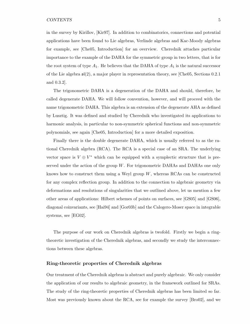
The dichotomy exhibited in the properties of SRAs - and therefore also of RCAs -
depending on the specialisation of the deformation parameter q is mirrored by a similar
dichotomy for DAHAs and trigonometric DAHAs. The DAHA is a PI algebra if the
deformation parameter q = 1, which is a result in [Obl04]. The trigonometric DAHA is a
PI algebra if and only if the deformation parameter q = 0, which was stated without proof
in [Obl04] and is proved in this thesis. The situation can be summarised in the following
table:
Cherednik algebra DAHA trigonometric DAHA RCA
Symbol H H H
Parameters tα, q tα, q tα, q
Parameter specialisations for which PI q = 1 q = 0 q = 0
Much of Cherednik’s work excludes the PI cases, because of the type of applications he is
interested in. Even when he considers DAHAs for q = 1, an additional relation between
the deformation parameters is imposed. An important feature in the study of Cherednik
algebras is the existence of faithful representations in terms of Dunkl-type operators, see
[Che05, Sections 2.12.2 - 2.12.4] for an overview. However, the representations mentioned
there are not faithful in the PI cases. Therefore, a limiting procedure has to be adopted
to deal with these cases, as was mentioned and proved for some examples in [Obl04]. See
also [Rou05, Section 5.1] for PI RCAs. In this thesis we will provide explicit descriptions
of faithful representations for almost all PI Cherednik algebras. These representations
provide us with embeddings of the PI Cherednik algebras into skew group algebras, which
will be our main tools in proving ring-theoretic results about the PI DAHA and the PI
trigonometric DAHA:
Result 1. Let H be a PI Cherednik algebra with parameter specialisation as in the table
above. Then there exists an embedding H → S[δ−1], where S is a certain nice skew group
algebra, which is well understood, and δ ∈ S. If H is a DAHA, there are some restrictions
on the Weyl group.
CONTENTS 7
Our aim was to obtain results for the general setup as well, where the deformation
parameters are not specialised. In this situation our results are more complete for the
trigonometric DAHA than the DAHA:
Result 2.
(i) The DAHA is prime and of infinite global dimension. If we specialise the DAHA
such that q = 1, then the PI DAHA is prime and noetherian. For most Weyl groups the
PI DAHA has finite GK dimension and its PI degree is |W |. If a point in its centre is
smooth then this point is Azumaya.
(ii) The trigonometric DAHA is noetherian, prime and has finite GK dimension and
finite global dimension. The PI trigonometric DAHA is noetherian, prime, has finite GK
and finite global dimension and has PI degree |W |. A point in its centre is smooth if and
only if this point is Azumaya.
Equivalences of Cherednik algebras
Understanding the connections between the Cherednik algebras is the second focal point
of our study. We have already mentioned that the Cherednik algebras are connected by a
process called degeneration which takes one from the DAHA to the trigonometric DAHA
and finally to the RCA. There is a second process, usually called completion, which reverses
the degeneration. These processes were first described by Lusztig in [Lus89] for the AHA
and the degenerate AHA. His techniques will be crucial for our work. Cherednik describes
the completion processes for the Cherednik algebras when they are not PI in [Che04, Sec-
tion 2]. This construction relies on the faithful representations of the Cherednik algebras
via Dunkl-type operators, which are invalid in the PI cases. If the Cherednik algebras are
not PI, then Cherednik’s construction implies that there is a natural equivalence of the
categories of finite dimensional modules for the RCA, the trigonometric DAHA and the
DAHA, see [BEG03, Proposition 7.1]. Thus the processes of degeneration and completion
provide equivalences that can be used to transfer results between the algebras.
It is our aim to take a first step towards filling the gap by investigating equivalences
between PI Cherednik algebras via the processes of degeneration and completion. In light
of the geometric application that we have in mind these cases are the ones of most relevance
to us. The idea is to achieve a level of understanding of these processes that enables us
to transfer across information that is known about the geometry of the centres of RCAs
from [EG02] and [Gor03a] to the trigonometric DAHA and the DAHA. In order to achieve
CONTENTS 8
this detailed understanding we will concentrate on the important and sufficiently small
examples of the Cherednik algebras attached to the symmetric group on two letters. In
these cases we are able to carry out all calculations very explicitly. We believe that the
degenerations and completions constructed in this document for the root system of type
A1 provide the required framework of equivalences and that it will be possible to generalise
them to most Weyl groups.
Result 3. Let W = S2.
(i) There exists a filtration of the DAHA H such that grH ∼= H, where H denotes the
trigonometric DAHA.
(ii) There exists a filtration of the trigonometric DAHA H such that grH ∼= H, where
H denotes the RCA.
We note that the degeneration process that we describe in this result is valid for the
general Cherednik algebras of type A1, not just for the PI cases.
Result 4. Let W = S2 and assume that we specialise the parameters of the Cherednik
algebras such that q = 1, q = 0, q = 0.
(i) For appropriate completions, H and H, we have
H ∼= H.
(ii) For appropriate completions, H and H, we have H ∼= H.
The key tools in constructing completions of the PI Cherednik algebras are the em-
beddings into skew group algebras that we constructed for PI Cherednik algebras. In
fact, we construct completions between the relevant skew group algebras and then restrict
them to the Cherednik algebras, a strategy that is outlined by Lusztig in [Lus89]. In both
the degeneration and the completion process we will need two steps to proceed from the
RCA to the DAHA and will always use the trigonometric DAHA as a connecting element.
Cherednik and Ostrik sketch a direct process to move between the RCA and the DAHA,
see [CO03], for specialisations where these algebras are not PI algebras. We were not able
to find an equivalent process for the PI case. There exist two distinct presentations for
trigonometric DAHAs, one of which is more suitable for constructing equivalences with
the RCA whereas the other is instrumental in finding the equivalences with the DAHA.
Since we utilize the trigonometric DAHA as an intermediate step for both the degenera-
tion and completion processes, we require embeddings of the trigonometric DAHA for both
presentations. An overview over the presentations and embeddings for the PI Cherednik
algebras of type A1 is given in the table in Appendix A.
CONTENTS 9
Furthermore, we divide our treatment of completions of Cherednik algebras into two
cases. In Gordon’s work in [Gor03a] a nice central subalgebra of an RCA is used to show
that the centre of some PI RCAs is always singular. The singularity always appears at
the origin of the variety corresponding to this nice central subalgebra. For the purpose
of constructing our completions we also use nice central subalgebras of the PI Cherednik
algebras. Thus with our geometric application in mind it is natural to investigate com-
pletions at the maximal ideals corresponding to the origins of these varieties first. To
complete the picture we secondly consider completions at arbitrary maximal ideals of the
relevant central subalgebras.
Graded Hecke algebras
In this thesis we are also concerned with graded Hecke algebras. These algebras were first
described by Drinfeld in [Dri86] and then studied in detail by Ram and Shepler in [RS03].
Drinfeld calls these algebras degenerate AHAs, but Ram and Shepler show that they are
true generalisations of the degenerate AHAs defined by Lusztig in [Lus89]. Therefore, we
will use the name graded Hecke algebras created by Ram and Shepler. Recently, in [Wit05]
Witherspoon has generalised these algebras even further by constructing twisted graded
Hecke algebras.
The ingredients for a graded Hecke algebra are a finite dimensional vector space V over
C and a finite subgroup of GL(V ). One then considers deformations of the skew group
algebra S(V ) ∗ G. We observe that S(V ) = C[V ∗], the coordinate ring of the complex
affine algebraic variety V ∗. Such a deformation is called a graded Hecke algebra if it
satisfies a PBW property similar to the one for SRAs. This means that the graded Hecke
algebra, A say, is a filtered algebra such that grA ∼= S(V ) ∗ G. Ram and Shepler show
very explicitly in [RS03, Section 3] that Lusztig’s degenerate AHAs are examples of graded
Hecke algebras. Whereas in Lusztig’s construction the structure of a finite real reflection
group is required, the construction of Drinfeld attaches a graded Hecke algebra to any
complex reflection group. One hopes that such algebras could be helpful instruments
in exploring the representation theory of the corresponding groups in the same way as
degenerate AHAs have been in the representation theory of Weyl groups. In their paper
mentioned above Ram and Shepler provide a classification of all graded Hecke algebras for
finite real and complex reflection groups. Suprisingly, there are complex reflection groups
CONTENTS 10
for which no nontrivial graded Hecke algebras exist.
The definition of graded Hecke algebras can also be motivated by deformation theory
as they are precisely the PBW deformations of S(V ) ∗G of a certain kind. This approach
gives an explanation for the choice of the construction of graded Hecke algebras. Moreover,
it is helpful in understanding the algebraic structure of graded Hecke algebras. A clue as
to what structure one might expect stems from the fact that one can view graded Hecke
algebras as generalisations of SRAs. Namely, if the vector space V possesses a symplectic
structure and the group G preserves this structure, then SRAs appear naturally as special
cases of graded Hecke algebras. Thus the obvious question to ask is whether graded
Hecke algebras display the same dichotomy as SRAs in their behaviour depending on
specialisations of the deformation parameters. More precisely, the question is whether
there are certain specialisations of the deformation parameters for which graded Hecke
algebras have large centres such that they are finitely generated over their centres and are
consequently PI. The purpose of our work is to find an answer to this question. If the
answer is affirmative, then these algebras again become of interest in non-commutative
algebraic geometry, in the same vein as SRAs.
We recall that an SRA is a PI algebra if and only if the parameter q = 0. This is a result
of [EG02, Theorem 3.1] and [BG03, Proposition 7.2]. As it turns out there is more than
one deformation parameter which controls whether or not graded Hecke algebras are PI.
We denote these parameters by q1, . . . , qN . This makes the case of graded Hecke algebras
more complicated than that of SRAs. The reason for this lies in the additional symplectic
structure that is available in the case of SRAs. When studying SRAs one can reduce
to the situation where V is a symplectic vector space such that V does not admit any
non-degenerate G-invariant subspaces. For such a vector space the space of G-invariant
antisymmetric bilinear forms on V , ((∧2 V )∗)G, is one-dimensional. This dimension gives
rise to the one parameter q, the specialisation of which determines whether an SRA is
PI or not. In general, when no additional structure is imposed on V , the dimension of
the space ((∧2 V )∗)G can be greater than one, say N . This leads to the appearance of N
deformation parameters qi. We show
Result 5. A graded Hecke algebra is PI if and only if qi = 0 for all i = 1, . . . , N .
Our work relies heavily on the results in [EG02] and [BG03, Proposition 7.2] and the
techniques developed in [EG02]. We have to make modifications though to account for
the fact that we maintain a general setup and do not assume a symplectic structure. Our
CONTENTS 11
results confirm a claim made by Etingof and Ginzburg in [EG02, Remark (ii) in Section
1] and we also give precise conditions for this claim.
Structure of the thesis
The structure of this document is as follows. In Chapter 1 we give definitions and results
that we will assume as background material in what follows. Chapter 2 contains the
definitions of the Cherednik algebras. Here we also prove basic ring-theoretic properties
and facts about homological dimensions for these algebras. We place emphasis on the
PI Cherednik algebras in preparation for Chapter 3. Result 1 is contained in Theorems
2.1.10 and 2.2.14 and Proposition 2.3.6. Part (i) of Result 2 is a summary of results in
Sections 2.1.1 and 2.1.2, Part (ii) can be found in Sections 2.2.1 and 2.2.2. In Chapter 3
we concentrate on the root system of type A1. In this setting we construct equivalences
between PI Cherednik algebras via the processes of degeneration and completion. The
theorems in Sections 3.2.1 and 3.2.2 are combined in Result 3. The details of Result
4 can be found in Theorems 3.3.3, 3.3.11, 3.3.15 and 3.3.22. We conclude the chapter
with an outline of the potential application of the constructed equivalences to algebraic
geometry. In the last chapter we describe our research into graded Hecke algebras and
provide detailed proofs of the results in [EG02] that we use. Corollary 4.5.5 is Result 5.
Chapter 1
Notation and preliminaries
We begin by introducing various definitions and concepts that will occur throughout the
remaining chapters. The main references for non-commutative ring theory are [MR87]
and [GW89]. For commutative algebra and algebraic geometry we use [Eis95] and [Har77].
Some results on invariant rings are taken from [Ben93]. Furthermore, references will be
provided within each of the following sections.
1.1 Localisations of non-commutative rings
A central part of our work is to determine whether or not certain algebras are noetherian
or prime. When we speak of a non-commutative ring being noetherian, we mean that it
is both right and left noetherian, unless we state otherwise. There are some easy ways of
deducing that a ring is noetherian:
Theorem 1.1.1. [GW89, Chapter 1] Let B be a ring.
(i) If B is commutative and finitely generated over C, then B is noetherian.
(ii) If B is noetherian, then any factor ring of B is also noetherian.
(iii) If B is a finitely generated module over a commutative noetherian subring, then
B is noetherian.
In addition to these facts, we will use localisations of the algebras in question and as-
sociated graded techniques to prove the properties of being noetherian or prime. The
subsequent definitions and results on localisation of non-commutative rings are taken
from [GW89, Chapter 9].
Let B be a non-commutative ring and let C be a multiplicatively closed subset of B.
12
CHAPTER 1. NOTATION AND PRELIMINARIES 13
Definition 1.1.2. A right localisation of B with respect to C (or a right quotient ring of
B with respect to C) is a ring Q together with a ring homomorphism θ : B → Q such that
(i) θ(c) is a unit in Q for all c ∈ C,
(ii) each element of Q has the form θ(b)θ(c)−1 for some b ∈ B, c ∈ C,
(iii) ker(θ) = b ∈ B | bc = 0 for some c ∈ C.
The definition of a left localisation is analogous. If a right localisation exists, then it
is unique. We usually write B[C−1] for Q, and we will later omit the word ‘right’ and just
speak of a localisation of B with respect to C. Let m denote a prime ideal of B. Then
C = b ∈ B | b + m is regular inB/m is a multiplicatively closed set in B and we write
B[C−1] = Bm. The conditions for the existence of a localisation of B can be summarised
as follows.
Theorem 1.1.3.
(i) A right localisation of B with respect to C exists if and only if C is a right denomi-
nator set if and only if C is a right Ore set which is right reversible.
(ii) If C consist of central nonzero divisors in B, then C is a right denominator set and
B embeds into B[C−1].
(ii) If B is right noetherian, then any right Ore set in B is right reversible and thus a
right denominator set.
(iii) [BR75] If B is noetherian and prime and b ∈ B is a nonzero divisor such that the
derivation [b,−] is nilpotent, then the set C = 1, b, b2, b3 . . . is a right denominator set.
Definition 1.1.4. Let C be a right denominator set in B and let M be a right B-module.
The localisation of M with respect to C (or the module of fractions of M with respect to C)
is the B[C−1]-module M [C−1] together with a B-module homomorphism φ : M →M [C−1]
such that
(i) each element of M [C−1] has the form φ(m)φ(c)−1 for some m ∈M , c ∈ C,
(ii) ker(φ) = m ∈M |mc = 0 for some c ∈ C.
The results summarised in the next theorem will allow us to deduce properties of the
localisation B[C−1] from properties of the algebra B.
Theorem 1.1.5. Let C be a right denominator set in B and M a right B-module.
(i) The map M ⊗B B[C−1] → M [C−1] given by m ⊗ s 7→ (m1−1) · s, for m ∈ M ,
s ∈ B[C−1], is a B[C−1]-module isomorphism.
CHAPTER 1. NOTATION AND PRELIMINARIES 14
(ii) If M ′ is another right B-module and f : M → M ′ is an injective B-module map,
then the induced map
f ⊗ 1 : M ⊗B B[C−1] →M ′ ⊗B B[C−1]
is injective. In other words, B[C−1] is a flat left B-module.
(iii) If M is noetherian then so is M [C−1].
(iv) If B is noetherian and prime then so is B[C−1].
For localisations of commutative rings see [Eis95, Chapter 2]. In particular, the above
theorem also holds if B is a commutative ring.
1.2 Associated graded algebras
See [MR87, Sections 1.6 and 7.6] for the following.
Definition 1.2.1. A ring B is Z-graded if there exist subgroups Bi, i ∈ Z, such that
(i) BiBj ⊆ Bi+j for all i, j ∈ Z,
(ii)⊕
i∈ZBi = B as an abelian group.
The elements of Bi are called homogeneous elements of degree i.
Definition 1.2.2. A ring B is said to be Z-filtered if there exist subgroups F iB, i ∈ Z such
that
(i) F iBFjB ⊆ F i+jB for all i, j ∈ Z,
(ii) F iB ⊆ F jB whenever i < j,
(iii)⋃i∈Z F
iB = B,
(iv)⋂i∈Z F
iB = 0.
The set F •B = F iB | i ∈ Z is called a filtration of B. If Bi = 0 for all i < 0, or if F iB = 0
for all i < 0, one says that B is positively graded or has a positive filtration, respectively.
In this thesis we mostly use positive gradings and filtrations. It is usually clear from the
context which kind of grading or filtration it is. Note that the filtration, as defined above,
is an increasing filtration.
If B is a filtered ring we can construct a graded ring from it which is called the
associated graded ring of B with respect to the filtration F •B and denoted by grFB:
grFB :=⊕i∈Z
F iBF i−1B
.
CHAPTER 1. NOTATION AND PRELIMINARIES 15
Take b := b + F i−1 ∈ grFB and b′ := b′ + F j−1 ∈ grFB, then b · b′ := bb′ + F i+j−1. If
b ∈ F iB/Fi−1B then b is said to have degree i.
Similarly we have filtered modules:
Definition 1.2.3. Suppose the ring B is Z-filtered. Let M be a right B-module. Then
M is said to be a Z-filtered B-module if there exist subgroups F iM , i ∈ Z, such that
(i) F iMFjB ⊆ F i+jM for all i, j ∈ Z,
(ii) F iM ⊆ F jM whenever i < j,
(iii)⋃i∈Z F
iM = M ,
(iv)⋂i∈Z F
iM = 0.
We denote the filtration on M by F •M and construct the associated graded module of
M with respect to this filtration, denoted by grFM , in the same way as for the ring B
above.
These constructions enable us to use properties of grFB to prove properties of B.
Whenever we use the next theorem we speak of using associated graded techniques.
Theorem 1.2.4. Let B be a filtered ring with filtration F •B and let grFB denote the
associated graded ring of B under this filtration.
(i) If grFB is an integral domain or prime or noetherian then B is an integral domain
or prime or noetherian.
(ii) Assume that grFB is noetherian. Then gl dimB ≤ gl dim grFB.
(iii) If M is a filtered B-module with filtration F •M , and grFM is finitely generated
over grFB, then M is finitely generated as B-module.
Here gldim denotes the global dimension of a ring, which we define in Section 1.4
1.3 PI algebras
For this section we use [MR87, Section 13]. The expression PI algebra (or PI ring) is
short for polynomial identity algebra (or polynomial identity ring). The identities we are
concerned with are polynomials in Z〈x1, x2, . . .〉.
CHAPTER 1. NOTATION AND PRELIMINARIES 16
Definition 1.3.1. Let f := f(x1, x2, . . .) ∈ Z〈x1, x2, . . .〉. Then the algebra B is said to
satisfy the identity f if f(b1, b2, . . .) = 0 for all bi ∈ B. The algebra B is said to be a
polynomial identity algebra if it satisfies a monic polynomial in Z〈x1, x2, . . .〉.
Example 1. Clearly, all commutative algebras are PI algebras, because they satisfy the
polynomial x1x2 − x2x1 = 0. Furthermore, matrix rings over commutative rings are PI
rings, see [BG02, III.1.3].
There are some easy criteria for when an algebra is a PI algebra:
Theorem 1.3.2.
(i) A subring or a homomorphic image of a PI algebra is a PI algebra.
(ii) If an algebra B is finitely generated as a module over a commutative subalgebra
then B is a PI algebra.
(iii) [BG02, Example I.13.2 (6)] If C be a right denominator set in B and B is a PI
algebra, then the localisation B[C−1] is also a PI algebra.
The converse to Part (ii) of this theorem does not hold in general, but we have:
Theorem 1.3.3. If B is a prime PI ring with centre Z(B) and Z(B) is noetherian, then
B is finitely generated as a Z(B)-module.
A PI algebra B is said to have minimal degree d if d is the least possible degree of a
monic polynomial identity of B.
Theorem 1.3.4. [Posner’s theorem] Suppose B is a prime PI ring with centre Z(B) and
minimal degree d. Let C = Z(B) \ 0. Let B[C−1] denote the localisation of B at C, and
Q = Z(B)[C−1] the quotient field of Z(B). Then B[C−1] is a simple Q-algebra with centre
Q which is finite dimensional over Q. Moreover, dimQ
(B[C−1]
)= (d/2)2
Inspired by this theorem one defines the PI degree of a prime PI algebra of minimal
degree d to be d/2.
Theorem 1.3.5. [BG02, Theorem I.13.5] Let B be a prime affine C-algebra. Suppose B
is a PI algebra with PI degree n. Then any irreducible B-module M is finite-dimensional.
Moreover, for all simple B-modules M we have dimM ≤ n.
The following result is used in the proof of the previous theorem and will later also be
useful to us:
CHAPTER 1. NOTATION AND PRELIMINARIES 17
Theorem 1.3.6 (Artin-Tate lemma). Let K ⊆ Z ⊆ B be rings such that both K
and Z are central subrings of B. Moreover, assume that K is noetherian, B is an affine
K-algebra and finitely generated as Z-module. Then Z is an affine K-algebra.
1.4 Smoothness and Azumaya algebras
Let X be an irreducible affine algebraic variety over C. We denote the coordinate ring of
a variety by O(X). Every point P in the variety X corresponds to a maximal ideal mP
of O(X). We denote the set of maximal ideals of O(X) by MaxSpecO(X). Since we will
be concerned with the question whether points in an algebraic variety are smooth, the
following result is essential:
Theorem 1.4.1. [Har77, Theorem I.5.1] Let P be a point in the irreducible affine variety
X. Then X is smooth at P if and only if the localisation OmP is a regular local ring.
A point in X which is not smooth is called a singular point. A smooth variety is a
variety which is smooth at all points that it contains. The concept of a local ring being
regular is related to the global dimension of this ring. We recall the definition of global
dimension, see [MR87, Chapter 7]. Namely, let B be any noetherian ring. Then the
projective dimension of a right B-module M is defined to be the minimum of the lengths
of projective resolutions of M .
Definition 1.4.2. The global dimension of a noetherian ring B is the supremum of the
projective dimensions of all B-modules.
Note that we do not have to make a distinction between right and left global dimension,
because we assume that B is noetherian, see [MR87, 7.1.11]. This will be the case for most
of the algebras in this document.
Theorem 1.4.3.
(i) [Eis95, Theorem 19.12] A commutative noetherian local ring is regular if and only
if it has finite global dimension.
(ii) [MR87, Corollary 7.4.3] Let B be a commutative noetherian ring. Then, for all
maximal ideals m of B,
gl dimBm ≤ gl dimB.
In what follows we will be particularly interested in the case when an algebra B is
an affine C-algebra and a finitely generated module over its centre Z(B). We will try
CHAPTER 1. NOTATION AND PRELIMINARIES 18
to understand whether Z(B) is smooth and in this particular situation this question is
connected to the question of whether the elements of MaxSpecZ(B) are Azumaya. For a
definition of an Azumaya algebra see [BG02, Section III.1] For us the following result will
suffice:
Theorem 1.4.4. [BG02, Theorem III.1.6] Let B be an affine prime C-algebra such that
B is a finitely generated module over Z(B). Let d denote the PI degree of B. Let m ∈
MaxSpecZ(B). Then Bm is Azumaya over Zm if and only if B/mB has a unique simple
module of dimension d, that is B/mB ∼= Md(C).
Then B is an Azumaya algebra if Bm is Azumaya over Zm for all m ∈ MaxSpecZ(B).
We call m ∈ MaxSpecZ(B) an Azumaya point if Bm is Azumaya over Zm and denote the
set of all Azumaya points in MaxSpecZ(B) by AZ(B). Denote the set of singular points
in MaxSpecZ(B) by SZ(B).
Theorem 1.4.5. [BG02, Lemma III.1.8] Suppose that B is an affine prime C-algebra
such that B is a finitely generated module over Z(B). If gl dimB < ∞, then AZ(B) and
SZ(B) are disjoint.
Thus in the situation of the theorem every Azumaya point of MaxSpecZ(B) is smooth.
If the algebra B satisfies further conditions, it can be shown that a point in MaxSpecZ(B)
is smooth if and only if it is Azumaya, see [BG02, Theorem III.1.8].
1.5 Completions
For the following see [Eis95, Chapter 7]. In this thesis the completions of Cherednik alge-
bras allow us to deduce properties about the original algebras that we completed. However,
completions are useful in a geometric setting as well. The localisation of the coordinate
ring of a variety at a maximal ideal contains information about Zariski-open neighbour-
hoods of the corresponding point of the variety. But the completion of such a localisation
allows one to study properties of the variety in much smaller neighbourhoods of the point,
namely those in the ordinary topology induced from Cn.
Let B be a commutative ring and m an ideal of B. Then the m-adic filtration of B is
the descending filtration given by B ⊃ m ⊃ m2 ⊃ m3 ⊃ . . ..
CHAPTER 1. NOTATION AND PRELIMINARIES 19
Definition 1.5.1. The completion of B with respect to m is defined as the inverse limit
of the factor rings B/mi and denoted by Bm. That is
Bm := lim←−
(B/mi)
= x = (x1, x2, . . .) ∈∏i
B/mi |xj ≡ xi (modmi) for all j > i
Example 2. The most important example of a completion is the completion of a polynomial
ring, say B = C[b], at the maximal ideal m = 〈b〉. Then Bm is the formal power series
ring: Bm∼= C[[b]]. Note that for m = 〈bk〉, k > 1, or m = 〈b − λ〉, λ ∈ C, we also have
Bm∼= C[[b]].
If the natural map B → Bm given by b 7→ (b + m, b + m2, . . .), for all b ∈ B, is an
isomorphism, then we say that B is complete with respect to the m-adic filtration of B.
We summarise some important results on completions:
Theorem 1.5.2. Let B be a commutative noetherian domain, m CB, and let Bm denote
the completion of B with respect to m. Then
(i) B ⊆ Bm.
(ii) Bm is complete with respect to the ideal mBm, and Bm/miBm
∼= B/mi, for all i ≥ 0.
(iii) The elements of the multiplicatively closed set 1 + u |u ∈ mBm are units in Bm.
(iv) Bm is noetherian.
(v) If M is a finitely generated B-module, then the natural map
Bm ⊗B M → lim←−
(M/miM) =: Mm
is an isomorphism.
1.6 Skew group algebras and invariant rings
The main references for this section are [Pas89] and [Ben93].
Definition 1.6.1. Let B be a ring and G be a finite group such that there exists a group
homomorphism G → Aut(B). Then the skew group ring B ∗ G is the free left B-module
with a basis given by the elements of the group and multiplication defined by
gb = g(b)g,
for b ∈ B and g ∈ G.
CHAPTER 1. NOTATION AND PRELIMINARIES 20
Each element of B ∗G has a unique expression of the form∑
g∈G bgg, for some bg ∈ B.
Certain properties of B ∗G can be deduced from properties of B:
Theorem 1.6.2. Let B be a ring, G a finite group acting as automorphisms of B and
B ∗G the skew group ring.
(i) [Pas89, Proposition 1.6] If B is noetherian then B ∗G is noetherian.
(ii) [Pas89, Corollary 12.6] If B is prime and if G acts faithfully on B, then B ∗G is
prime.
(iii) [MR87, Theorem 7.5.6] Suppose B is noetherian and the order of G is a unit in
B. Then gl dimB = gl dim (B ∗G).
Assume that B is a commutative affine C-algebra and that G is a finite group acting
faithfully on B. Then it is easy to see that the centre of B ∗G is BG, the ring of elements
which are invariant under the action of the group G. This invariant ring and its relation
to the rings B and B ∗ G will play a role at different stages of our work. We have the
following two famous results:
Theorem 1.6.3 (Hilbert-Noether theorem). [Ben93, Theorem 1.3.1] Suppose that B
is a commutative affine C-algebra and that G is a finite group acting as automorphisms
of B. Then BG is also a commutative affine C-algebra and B is finitely generated as a
module over BG.
Let V be a finite dimensional vector space over C and let G ⊆ GL(V ) be a finite group.
Write C[V ] to denote the ring of polynomial functions on V , that is C[V ] = S(V ∗), the
symmetric algebra of the dual space V ∗. The action of G on V induces a faithful action of
G on V ∗ by setting (gf)(v) = f(g−1(v)), for all g ∈ G, v ∈ V and f ∈ V ∗. Moreover, the
action of G on V ∗ can be extended multiplicatively to an action of G on S(V ∗) = C[V ].
Recall that an element of G is called a reflection in its action on V if it does not act as
the identity on V and if it fixes a subspace of codimension one in V .
Theorem 1.6.4 (Chevalley-Shephard-Todd theorem). [Ben93, Theorem 7.2.1] [Hum90,
Theorem 3.5, Proposition 3.6] Suppose that V is a finite dimensional vector space over C
and that G ⊆ GL(V ) is a finite group. Let n denote the dimension of V . Then the
following are equivalent:
(i) G is generated by elements which act as reflections on V .
(ii) C[V ] is a free C[V ]G-module of rank |G|.
(iii) C[V ]G is a polynomial ring in n variables.
CHAPTER 1. NOTATION AND PRELIMINARIES 21
This theorem can be extended to Laurent polynomial rings. Note that the group
GLd(Z), the group of integer d× d matrices of determinant ±1, acts on the Laurent poly-
nomial ring C[X±11 , . . . , X±1
d ] via its natural action on the multiplicative group generated
by X1, . . . , Xd (∼= Zd). We have
Theorem 1.6.5. [Lor96] Suppose that G is a finite subgroup of GLd(Z) acting effectively
on B := C[X±11 , . . . , X±1
d ]. Then the following are equivalent:
(i) G is a reflection group.
(ii) B is free as a BG-module of rank |G|.
(iii) BG is a polynomial ring in d variables.
Let us return to the situation of a finite dimensional vector space V over C and a finite
group G ⊆ GL(V ). We recall some concepts from algebraic geometry which are relevant
in this situation:
Both V and V ∗ are irreducible smooth affine varieties. The coordinate ring of V ∗ is
denoted by O(V ∗) and we have O(V ∗) = S(V ) = C[V ∗]. Note that V ∗ is connected, since
it is irreducible, which implies that any two non-empty open subsets of V ∗ must intersect.
Furthermore, V ∗ is a normal variety, since O(V ∗) is integrally closed, see [Har77] for more
details.
Recall that the action of G on V induces an action of G on V ∗. We have G ⊆ GL(V ∗).
In other words, G is a linear algebraic group acting on the affine variety V ∗, see [FSR05,
Example 3.2.6]. Since G is a finite group and we are working over C, it is both a lin-
early and geometrically reductive group, see [FSR05, Corollary 9.2.7 and Theorem 9.2.8].
By [FSR05, Theorem 9.4.3], G is then reductive.
We have the quotient map
π : V ∗ → V ∗/G.
The coordinate ring of V ∗/G is O(V ∗/G) = S(V )G, [New78, Theorem 3.5]. By the Hilbert-
Noether theorem, S(V ) is finitely generated as a module over its subalgebra S(V )G and
noetherian, because S(V )G is a commutative affine C-algebra and thus noetherian, see
Theorem 1.1.1. Therefore, the map π is a finite map, see [Dre04, Definition 1.1], which
implies that π is a closed map, see [Dre04, Proposition 1.2], that is π takes closed subsets
CHAPTER 1. NOTATION AND PRELIMINARIES 22
to closed subsets. By [Dre04, Theorem 2.17 and Definition 2.18] the space V ∗/G is then
a good quotient of V ∗ by G and also a geometric quotient.
Chapter 2
Cherednik algebras
In this chapter we describe the algebras which we subsume under the name Cherednik
algebras. These are the double affine Hecke algebra (DAHA), the trigonometric double
affine Hecke algebra and the rational Cherednik algebra (RCA). There are two sections
for each of these algebras. In the first of these sections we give some background material
on root systems, the definition of the algebra and a PBW basis. In addition, for the
trigonometric DAHA and the DAHA we attempt to show the following ring-theoretic
properties:
• The algebra is noetherian.
• The algebra is prime.
• Determine whether the algebra has finite global dimension.
We also provide a very useful embedding for the trigonometric DAHA into a skew group
algebra.
In the second section for each of the Cherednik algebras we concentrate on the cases in
which they are PI algebras. Here we consider the following properties for the trigonometric
DAHA and the DAHA:
• The algebra is noetherian and prime.
• An embedding of the algebra into a skew group algebra.
• Determine the PI degree of the algebra.
• Describe the centre of the algebra.
• Determine whether points in the centre of the algebra are smooth if and only if they
are Azumaya.
The sections on the RCA are mainly expository and will contain information on the same
properties.
23
CHAPTER 2. CHEREDNIK ALGEBRAS 24
2.1 The double affine Hecke algebra
2.1.1 Definition and first properties
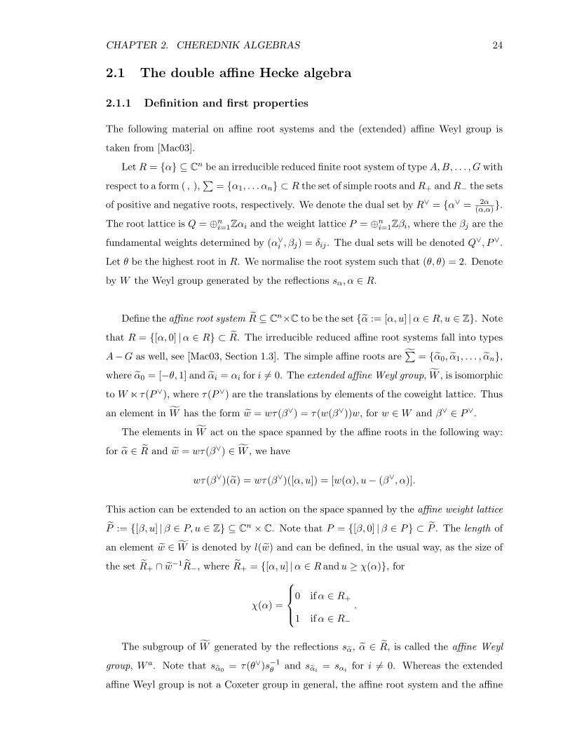
The following material on affine root systems and the (extended) affine Weyl group is
taken from [Mac03].
Let R = α ⊆ Cn be an irreducible reduced finite root system of type A,B, . . . , G with
respect to a form ( , ),∑
= α1, . . . αn ⊂ R the set of simple roots and R+ and R− the sets
of positive and negative roots, respectively. We denote the dual set by R∨ = α∨ = 2α(α,α).
The root lattice is Q = ⊕ni=1Zαi and the weight lattice P = ⊕ni=1Zβi, where the βj are the
fundamental weights determined by (α∨i , βj) = δij . The dual sets will be denoted Q∨, P∨.
Let θ be the highest root in R. We normalise the root system such that (θ, θ) = 2. Denote
by W the Weyl group generated by the reflections sα, α ∈ R.
Define the affine root system R ⊆ Cn×C to be the set α := [α, u] |α ∈ R, u ∈ Z. Note
that R = [α, 0] |α ∈ R ⊂ R. The irreducible reduced affine root systems fall into types
A−G as well, see [Mac03, Section 1.3]. The simple affine roots are∑
= α0, α1, . . . , αn,
where α0 = [−θ, 1] and αi = αi for i 6= 0. The extended affine Weyl group, W , is isomorphic
to W n τ(P∨), where τ(P∨) are the translations by elements of the coweight lattice. Thus
an element in W has the form w = wτ(β∨) = τ(w(β∨))w, for w ∈W and β∨ ∈ P∨.
The elements in W act on the space spanned by the affine roots in the following way:
for α ∈ R and w = wτ(β∨) ∈ W , we have
wτ(β∨)(α) = wτ(β∨)([α, u]) = [w(α), u− (β∨, α)].
This action can be extended to an action on the space spanned by the affine weight lattice
P := [β, u] |β ∈ P, u ∈ Z ⊆ Cn × C. Note that P = [β, 0] |β ∈ P ⊂ P . The length of
an element w ∈ W is denoted by l(w) and can be defined, in the usual way, as the size of
the set R+ ∩ w−1R−, where R+ = [α, u] |α ∈ R andu ≥ χ(α), for
χ(α) =
0 ifα ∈ R+
1 ifα ∈ R−.
The subgroup of W generated by the reflections sα, α ∈ R, is called the affine Weyl
group, W a. Note that sα0= τ(θ∨)s−1
θ and sαi= sαi for i 6= 0. Whereas the extended
affine Weyl group is not a Coxeter group in general, the affine root system and the affine
CHAPTER 2. CHEREDNIK ALGEBRAS 25
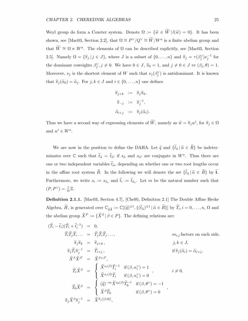
Weyl group do form a Coxeter system. Denote Ω := w ∈ W | l(w) = 0. It has been
shown, see [Mac03, Section 2.2], that Ω ∼= P∨/Q∨ ∼= W/W a is a finite abelian group and
that W ∼= Ω n W a. The elements of Ω can be described explicitly, see [Mac03, Section
2.5]. Namely Ω = πj | j ∈ J, where J is a subset of 0, . . . , n and πj = τ(β∨j )ν−1j for
the dominant coweights β∨j , j 6= 0. We have 0 ∈ J , π0 = 1, and j 6= 0 ∈ J ⇔ (βj , θ) = 1.
Moreover, νj is the shortest element of W such that νj(β∨j ) is antidominant. It is known
that πj(α0) = αj . For j, k ∈ J and i ∈ 0, . . . , n one defines
πj+k := πj πk,
π−j := π−1j ,
αi+j := πj(αi).
Thus we have a second way of expressing elements of W , namely as w = πjw′, for πj ∈ Ω
and w′ ∈W a.
We are now in the position to define the DAHA. Let q and tα | α ∈ R be indeter-
minates over C such that tα = tα′ if sα and sα′ are conjugate in W a. Thus there are
one or two independent variables tα, depending on whether one or two root lengths occur
in the affine root system R. In the following we will denote the set tα | α ∈ R by t.
Furthermore, we write si := sαiand ti := tαi
. Let m be the natural number such that
(P, P∨) = 1mZ.
Definition 2.1.1. [Mac03, Section 4.7], [Che95, Definition 2.1] The Double Affine Hecke
Algebra, H, is generated over Cq,t := C[(q)±1, (tα)±1 | α ∈ R] by Ti, i = 0, . . . , n, Ω and
the abelian group XP := Xβ |β ∈ P. The defining relations are:
(Ti − ti)(Ti + t−1i ) = 0,
TiTjTi . . . = TjTiTj . . . , mi,j factors on each side,
πj πk = πj+k , j, k ∈ J,
πjTiπ−1j = Ti+j , if πj(αi) = αi+j ,
XβXβ′ = Xβ+β′ ,
TiXβ =
Xsi(β)T−1i if (β, α∨i ) = 1
Xsi(β)Ti if (β, α∨i ) = 0, i 6= 0,
T0Xβ =
(q)−mXsθ(β)T−10 if (β, θ∨) = −1
XβT0 if (β, θ∨) = 0,
πjXβπ−1
j = X πj([β,0]),
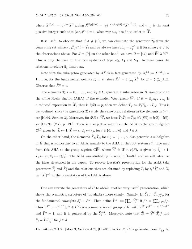
CHAPTER 2. CHEREDNIK ALGEBRAS 26
where X [β,u] := (q)muXβ giving X πj([β,0]) = (q)−m(β,νj(β∨j ))Xν−1
j (β), and mi,j is the least
positive integer such that (sisj)mi,j = 1, whenever sisj has finite order in W .
It is useful to observe that if J 6= 0, we can eliminate the generator T0 from the
generating set, since π−j Tj π−1−j = T0 and we always have π−j = π−1
j ∈ Ω for some j ∈ J by
the observations above. For J = 0 on the other hand, we have Ω = id and W ∼= W a.
This is only the case for the root systems of type E8, F4 and G2. In these cases the
relations involving πj disappear.
Note that the subalgebra generated by XP is in fact generated by X±1i := X±βi , i =
1, . . . , n, for the fundamental weights βi in P , since Xβ =∏ni=1 X
λii for β =
∑ni=1 λiβi.
Observe that X0 = 1.
The elements Ti, i = 0, . . . , n, and πj ∈ Ω generate a subalgebra in H isomorphic to
the affine Hecke algebra (AHA) of the extended Weyl group W . If w = πjsi1 . . . sip is
a reduced expression in W , that is l(w) = p, then we define Tw := πjTi1 . . . Tip . This is
well-defined, since the generators Ti satisfy the same braid relations as the elements in W a,
see [Kir97, Section 3]. Moreover, for w, v ∈ W , we have TwTv = Twv if l(wv) = l(w)+ l(v),
see [Che95, (2.7), p. 199]. There is a surjective map from the AHA to the group algebra
CW given by: ti 7→ 1, Ti 7→ si, πj 7→ πj , for i ∈ 0, . . . , n and j ∈ J .
On the other hand, the elements Xi, Tj , for i, j = 1, . . . , n, also generate a subalgebra
in H that is isomorphic to an AHA, namely to the AHA of the root system R∨. The map
from this AHA to the group algebra CW , where W ∼= W n τ(P ), is given by tj 7→ 1,
Tj 7→ sj , Xi 7→ τ(βi). The AHA was studied by Lusztig in [Lus89] and we will later use
the ideas developed in his paper. To recover Lusztig’s presentation for the AHA take
generators T ′i and X ′i and the relations that are obtained by replacing Ti by t−1i T ′i and Xi
by (X ′i)−1 in the presentation of the DAHA above.
One can rewrite the generators of H to obtain another very useful presentation, which
shows the symmetric structure of the algebra more clearly. Namely, let Yi := Tτ(β∨i ), for
the fundamental coweights β∨i ∈ P∨. Then define Y β∨ :=∏ni=1 Y
µii if β∨ =
∑ni=1 µiβ
∨i .
Thus Y P∨ := Y β∨ |β∨ ∈ P∨ is a commutative subgroup of H, with Y β∨ Y β′∨ = Y β∨+β′∨
and Y 0 = 1, and it is generated by the Y ±1i . Moreover, note that T0 = Y θ∨ T−1
sθand
πj = YjT−1νj
for j ∈ J .
Definition 2.1.2. [Mac03, Section 4.7], [Che95, Section 2] H is generated over Cq,t by
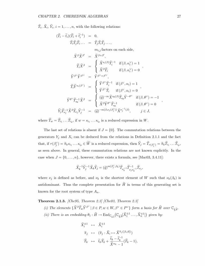
CHAPTER 2. CHEREDNIK ALGEBRAS 27
Ti, Xi, Yi, i = 1, . . . , n, with the following relations:
(Ti − ti)(Ti + t−1i ) = 0,
TiTjTi . . . = TjTiTj . . . ,
mi,j factors on each side,
XβXβ′ = Xβ+β′ ,
TiXβ =
Xsi(β)T−1i if (β, α∨i ) = 1
XβTi if (β, α∨i ) = 0,
Y β∨ Y β′∨ = Y β∨+β′∨ ,
TiYsi(β
∨) =
Y β∨ T−1i if (β∨, αi) = 1
Y β∨ Ti if (β∨, αi) = 0,
Y θ∨ T−1sθXβ =
(q)−mXsθ(β)TsθY −θ
∨if (β, θ∨) = −1
XβY θ∨ T−1sθ
if (β, θ∨) = 0,
YjT−1νjXβTνj Y
−1j = (q)−m(β,νj(β
∨j ))Xν−1
j (β), j ∈ J,
where Tw = Ti1 . . . Tip , if w = si1 . . . sip is a reduced expression in W .
The last set of relations is absent if J = 0. The commutation relations between the
generators Yj and Xi can be deduced from the relations in Definition 2.1.1 and the fact
that, if τ(β∨j ) = πksi1 . . . sip ∈ W is a reduced expression, then Yj = Tτ(β∨j ) = πkTi1 . . . Tip ,
as seen above. In general, these commutation relations are not known explicitly. In the
case when J = 0, . . . , n, however, there exists a formula, see [Mac03, 3.4.11]:
X−1k Y −1
j XkYj = (q)m(β∨j ,βk)Tν−1kT−1
νjν−1k
Tνj ,
where νj is defined as before, and νk is the shortest element of W such that νk(βk) is
antidominant. Thus the complete presentation for H in terms of this generating set is
known for the root system of type An.
Theorem 2.1.3. [Che95, Theorem 2.3] [Che03, Theorem 2.3]
(i) The elements XβTwYβ∨ |β ∈ P,w ∈W,β∨ ∈ P∨ form a basis for H over Cq,t.
(ii) There is an embedding θ1 : H → EndCq,t
(Cq,t[X
±11 . . . , X±1
n ])
given by:
X±1i 7→ X±1
i
πj 7→ (πj : Xi 7→ X πj([βi,0]))
Tk 7→ tkTk +tk − t−1
k
Xαk − 1(Tk − 1),
CHAPTER 2. CHEREDNIK ALGEBRAS 28
where j ∈ J and Tk, k = 0, . . . , n, acts on Cq,t[X±11 , . . . , X±1
n ] by Xi 7→ Xsk(βi). This map
remains faithful when the ti are specialised to arbitrary values in C∗ and q to an element
in C∗ that is not a root of unity.
Thus we have H ∼= Cq,t[X±11 , . . . , X±1
n ] ⊗Cq,tHfin
q,t⊗Cq,t
Cq,t[Y±11 , . . . , Y ±1
n ] as Cq,t -
modules, where Hfin
q,tis the finite Hecke algebra for the root system R defined over Cq,t.
We call this basis as Cq,t -module the PBW basis of H. From [Che03, Theorem 2.3] we
also know that there are five more Cq,t -module isomorphisms analogues to this, which
correspond to the other orders of Xβ, Tw and Y β∨ in the basis. For a detailed account of
the theory of finite Hecke algebras see [GP00].
Whenever we write H we refer to the DAHA defined over Cq,t, with q and the elements
of t indeterminates. If we want to specialise these indeterminates to complex numbers, we
will use different notation to emphasise this.
We claim that the DAHA is a deformation of a skew group algebra. Namely, consider
the factor of H by the ideal 〈t1 − 1, . . . , tn − 1, q − 1〉H. In other words, specialise all
parameters in t and q to 1. Note that the parameter q appears in the relations of the
DAHA only to powers that are multiples of m, where m ∈ Z is the least natural number
such that (P, P∨) = 1mZ. Thus a specialisation of q such that (q)m = 1 works as well.
It is clear that this factor algebra is isomorphic to the C-algebra generated by Ti, Xi, Yi,
i = 1, . . . , n, with the following relations:
T 2i = 0,
TiTjTi . . . = TjTiTj . . . , mi,j factors on each side,
XiXj = XjXi,
TiXj = Xsi(βj)Ti,
YiYj = Yj Yi,
TiYj = Y si(β∨j )Ti,
XiYj = YjXi,
where mi,j is the least positive integer such that (sisj)mi,j = 1 ∈ W . This follows from
the presentation of the DAHA in Definition 2.1.2 and the fact that one can obtain the
CHAPTER 2. CHEREDNIK ALGEBRAS 29
commutation relations between Xi and Yk for all k = 1, . . . , n by conjugating the relation
for Xi and Y θ by Tw for some w ∈ W . Thus H/〈t1 − 1, . . . , tn − 1, q − 1〉H is the skew
group algebra C[X±1, Y ±1] ∗W , where C[X±1, Y ±1] := C[X±11 , . . . , X±1
n , Y ±11 , . . . , Y ±1
n ].
Let us now begin a ring-theoretic study of the DAHA. Unfortunately, there is no
obvious filtration on the DAHA which would allow one to use associated graded techniques
as described in Theorem 1.2.4. Instead we use the fact that the DAHA is related to a skew
group algebra, as described above, to deduce properties of the DAHA from properties of
the skew group. We require the following well-known lemma:
Lemma 2.1.4. Let B be an algebra containing a central element b such that:
(i) B/bB is prime,
(ii) b is a nonzero divisor in B,
(iii)⋂∞n=0 b
nB = 0.
Then B is prime.
Proof. Let I, J be nonzero ideals of B such that IJ = 0. Then by assumption (iii) there
exist n,m ≥ 0 such that
I ⊆ bnB, I * bn+1B,
J ⊆ bmB, J * bm+1B.
Let I ′ := x ∈ B | bnx ∈ I, which is an ideal of B since b is central, and define J ′ similarly.
Then I = bnI ′, J = bmJ ′ and 0 = IJ = bn+mI ′J ′, since b is central. Thus (ii) implies
I ′J ′ = 0. We have I ′ * bB and J ′ * bB and thus two nonzero ideals of B/bB that multiply
to zero, namely (I ′ + bB)/bB and (J ′ + bB)/bB, a contradiction to assumption (i).
Proposition 2.1.5. H is prime.
Proof. We will show that the DAHA is prime for the parameter specialisation such that
q = 1 and ti = 1 for all i = 1, . . . , n. The result then follows by using the above lemma
iteratively, since both q − 1 and ti − 1 are central nonzero divisors in H, as can be seen
from the PBW basis for H in the previous theorem. Moreover,⋂∞n=0(ti − 1)nH = 0 and⋂∞
n=0(q−1)nH = 0, since the PBW theorem for H implies that H is a free Cq,t-module and
since the Krull intersection theorem, see [Eis95, Corollary 5.4], holds for the noetherian
domain Cq,t. This remains true if we specialise the other parameters to 1 first. But, as we
saw earlier, H/〈t1 − 1, . . . , tn − 1, q − 1〉H ∼= C[X±1, Y ±1] ∗W and this algebra is prime
by Theorem 1.6.2, since W acts faithfully on the commutative domain C[X±1, Y ±1].
CHAPTER 2. CHEREDNIK ALGEBRAS 30
Remark 2.1.6. The argument used in this proof also shows that the DAHA is prime if we
specialise the parameters such that (q)m = 1 and ti = 1 for all i = 1, . . . , n. Moreover, the
argument in the proof works if we only specialise q such that either (q)m = 1 or q = 1 and
leave the parameters in t as indeterminates.
Question 1. A very important and interesting problem is whether the DAHA is noethe-
rian. This is answered for the specialisation of q such that (q)m = 1 or q = 1 in the next
section, but it remains open for q an arbitrary parameter. Obviously, if one can show that
the DAHA is noetherian when q is an indeterminate, then this implies that the DAHA
is noetherian for all specialisations of q, since these specialisations are nothing else but
factor algebras, see Theorem 1.1.1.
Let us conclude this general section on the DAHA by considering the global dimension
of the DAHA. Since we do not know yet, whether the DAHA is noetherian we have to
differentiate between right and left global dimension. In the following we will always refer
to the right global dimension of the DAHA, see [MR87, 7.1.8]. We were again aiming to
answer the question whether the global dimension of the DAHA is finite for all possible
specialisations of the parameters t and q. However, so far we can only provide a partial
answer to this.
The Poincare polynomial for the finite Hecke algebra plays a crucial role. It is defined
as
P (t) =∑w∈W
(tw)2,
where tw = ti1 · · · tip if w = si1 · · · sip is a reduced expression. An explicit description of
the Poincare polynomial for all root systems can be found in [Gyo95, Section 3.4]. For
the root system of type An, for example, we have P (t) =∑
w∈W (t)2l(w), where l(w) is the
usual length function for the Weyl group W .
Proposition 2.1.7.
(i) The global dimension of H is infinite.
(ii) Specialise the indeterminates in t to complex numbers λα and denote the specialised
DAHA by Hλ. If P (t) evaluated at the complex numbers λα is zero, gldim Hλ = ∞.
Proof. The essential fact that we use is that the DAHA contains the finite Hecke algebra
over Cq,t, Hfin
q,t, and that H is free as a left and right Hfin
q,t-module by the PBW theorem
for H. Moreover, the basis of H as Hfin
q,t-module contains 1.
CHAPTER 2. CHEREDNIK ALGEBRAS 31
(i) If we can show that the global dimension of Hfin
q,tis infinite, then the result can be
deduced by the following argument. Assume gldimHfin
q,t= ∞. Pick an Hfin
q,t-module M
with infinite projective dimension. Then M := M ⊗Hfin
q,t
H is a right H-module. If we
consider M as anHfin
q,t-module by restriction, thenM ∼= M⊗
Hfin
q,t
Hfin
q,tis a direct summand
of M , because of the earlier observations about the basis of H as Hfin
q,t-module. Suppose
there exists a finite projective resolution of M as right H-module. This resolution is also
a finite projective resolution of M as Hfin
q,t-module by restriction from H to Hfin
q,t. Thus
the projective dimension of M as Hfin
q,t-module is finite, which implies that the projective
dimension of its direct summand M is finite, see [Rot79, Exercise 9.8], a contradiction.
Note that Hfin
q,t= C[q±1]⊗CH
fin
t, where Hfin
tis the usual finite multi-parameter Hecke
algebra. By the same argument as above it now suffices to show that gldimHfin
t= ∞.
Consider the subalgebra B of Hfin
tgenerated by T := Ti for some i = 1, . . . , n, thus let
B = Ct 〈 T | (T − t)(T + t−1) = 0〉, where t := ti and Ct = C[t±1]. The algebra B is in fact
the finite Hecke algebra for the root system A1. But the reflection si, which corresponds to
the generator Ti of B, generates a parabolic subgroup of W . Together with the fact that
Ct = C[t±1α | α ∈ R] is free as a Ct-module this implies that Hfin
tis a free left B-module,
see [GP00, 4.4.7]. Therefore, we can use the same argument as above once more to reduce
the problem further to showing that gldimB = ∞.
It is easy to see that the variety associated to B is not smooth using the Jacobian
criterion described in [Kun85, Theorem VI.1.15]. This implies that gldimB = ∞ by
Theorem 1.4.3. We want to use a different approach in this proof, however, as we believe
this approach reveals a recurring pattern. The Poincare polynomial for B is 1 + (t)2,
which is not invertible in Ct. Denote I := (T + t−1)B = (1 + t T )B, a two-sided ideal of
B, and denote the two-sided ideal of B generated by T − t by J . We have IJ = JI = 0.
Thus J ⊆ AnnBI. If J $ AnnBI then AnnBI ∩ (B/J) 6= 0. But B/J ∼= Ct and Ct \ 0
consists of nonzero divisors in B, by the PBW theorem for the finite Hecke algebra. Thus
we have J = AnnBI. On the other hand, I = AnnBJ , which follows from the fact
that B is a symmetric algebra: in [GP00, Proposition 8.1.1] a non-degenerate associative
symmetric bilinear form on B, say (−,−)B, is constructed. This form can be extended to
a non-degenerate associative symmetric bilinear form on B := B⊗CtQuot(Ct) by defining
(b⊗p, b′⊗p′)B := (b, b′)B pp′, for b, b′ ∈ B, p, p′ ∈ Quot(Ct), and extending bilinearly. Thus
B is a finite dimensional symmetric algebra over a field, and B is Frobenius because of the
form that we constructed, see [Row88, Exercise 3.3.29]. This in turn implies that B is quasi-
CHAPTER 2. CHEREDNIK ALGEBRAS 32
Frobenius, by [Rot79, Theorem 4.39]. Denote I := I⊗CtQuot(Ct) and J = J⊗Ct
Quot(Ct),
two-sided ideals of B. Then J = AnnB I implies that I is the left annihilator of J in B,
see [CR87a, Section 9A]. It now follows that AnnBJ = I ∩B = I.
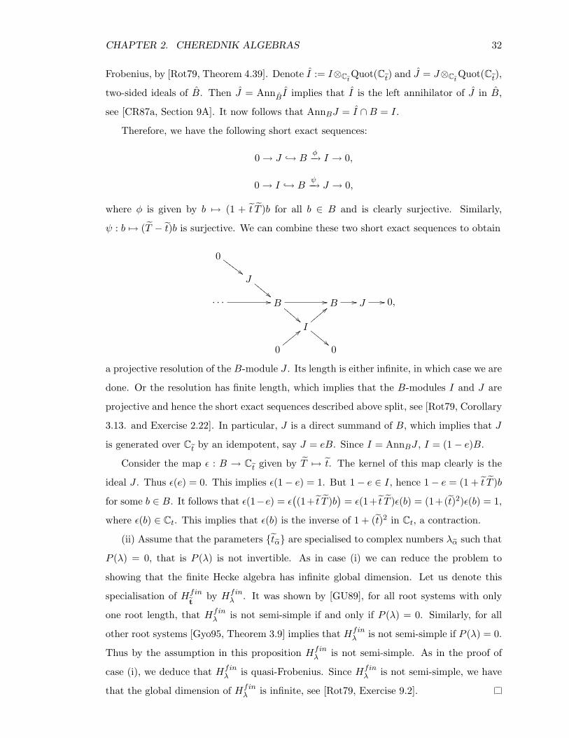
Therefore, we have the following short exact sequences:
0 → J → Bφ−→ I → 0,
0 → I → Bψ−→ J → 0,
where φ is given by b 7→ (1 + t T )b for all b ∈ B and is clearly surjective. Similarly,
ψ : b 7→ (T − t)b is surjective. We can combine these two short exact sequences to obtain
0##GGG
GGG
J
""EEEE
E
· · · // B //
!!DDDD
D B // J // 0,
I
==zzzzz
""EEEE
E
0
<<yyyyy0
a projective resolution of the B-module J . Its length is either infinite, in which case we are
done. Or the resolution has finite length, which implies that the B-modules I and J are
projective and hence the short exact sequences described above split, see [Rot79, Corollary
3.13. and Exercise 2.22]. In particular, J is a direct summand of B, which implies that J
is generated over Ct by an idempotent, say J = eB. Since I = AnnBJ , I = (1− e)B.
Consider the map ε : B → Ct given by T 7→ t. The kernel of this map clearly is the
ideal J . Thus ε(e) = 0. This implies ε(1− e) = 1. But 1− e ∈ I, hence 1− e = (1 + t T )b
for some b ∈ B. It follows that ε(1−e) = ε((1+ t T )b
)= ε(1+ t T )ε(b) = (1+(t)2)ε(b) = 1,
where ε(b) ∈ Ct. This implies that ε(b) is the inverse of 1 + (t)2 in Ct, a contraction.
(ii) Assume that the parameters tα are specialised to complex numbers λα such that
P (λ) = 0, that is P (λ) is not invertible. As in case (i) we can reduce the problem to
showing that the finite Hecke algebra has infinite global dimension. Let us denote this
specialisation of Hfin
tby Hfin
λ . It was shown by [GU89], for all root systems with only
one root length, that Hfinλ is not semi-simple if and only if P (λ) = 0. Similarly, for all
other root systems [Gyo95, Theorem 3.9] implies that Hfinλ is not semi-simple if P (λ) = 0.
Thus by the assumption in this proposition Hfinλ is not semi-simple. As in the proof of
case (i), we deduce that Hfinλ is quasi-Frobenius. Since Hfin
λ is not semi-simple, we have
that the global dimension of Hfinλ is infinite, see [Rot79, Exercise 9.2].
CHAPTER 2. CHEREDNIK ALGEBRAS 33
Question 2. Whether the polynomial P (t) is invertible in Cq,t seems to crucially influence
whether the global dimension of the DAHA is finite. Thus it makes sense to ask: Is
gldim H[P (t)−1] <∞? Does P (λ) 6= 0 imply gldim Hλ <∞?
2.1.2 The specialisation q = 1
In this section we restrict ourselves to the case when q = 1. We denote this specialisation
of H by H = H/〈q − 1〉H and write Ct = C[t±1α | α ∈ R]. As we observed before, the
results for the specialisation q = 1 also hold for all specialisations such that (q)m = 1,
where m is again the natural number such that (P, P∨) = 1mZ. This is because in the
definition of the DAHA the parameter q only ever occurs to powers that are multiples of
m. In the following, however, we will maintain the assumption of q = 1 and only mention
the more general case of (q)m = 1 if necessary. The following result provides the reason
for our particular interest in this specialisation:
Proposition 2.1.8. [Obl04, Lemma 5.2, Lemma 5.4]
(i) Z(H) ⊇ Ct[X±11 , . . . , X±1
n ]W , Z(H) ⊇ Ct[Y±11 , . . . , Y ±1
n ]W .
(ii) H is a finite module over the subalgebra Ct[X±11 , . . . , X±1
n ]W⊗CtCt[Y
±11 , . . . , Y ±1
n ]W .
Since H is finitely generated over a central subalgebra, it is a PI algebra, see Theorem
1.3.2. Therefore, we call the specialisation H the PI DAHA.
Question 3. It remains open whether the DAHA is a PI algebra if and only if (q)m = 1.
Corollary 2.1.9. H is noetherian.
Proof. We have by Proposition 2.1.8 that H is finitely generated over the central sub-
algebra Ct[X±11 , . . . , X±1
n ]W ⊗CtCt[Y
±11 , . . . , Y ±1
n ]W , which is commutative and finitely
generated over C by Theorem 1.6.5, and thus noetherian. This implies that H is noethe-
rian by Theorem 1.1.1.
We will now construct an embedding for the PI DAHA. Recall that the embedding
described in Theorem 2.1.3 assumes that q is not specialised to a root of unity. To find an
embedding for H we will use a technique that Lusztig developed for the AHA in [Lus89].
We have to assume, however, that J 6= 0 to be able to eliminate the generator T0 in
the presentation of Definition 2.1.1. Hence this embedding will not work for the following
root systems: E8, F4, G2.
CHAPTER 2. CHEREDNIK ALGEBRAS 34
Denote Ct[X±1, D±1] := Ct[X
±11 , . . . , X±1
n , D±11 , . . . , D±1
n ], a commutative Laurent
polynomial ring. We define the following skew group algebra S := Ct[X±1, D±1] ∗ W ,
where the generators of the Weyl group W are denoted by T1, . . . , Tn. The multiplication
is given by
TkXi = Xsk(βi)Tk and TkDj = Dsk(β∨j )Tk,
where Xβ =∏ni=1 X
λii for β =
∑ni=1 λiβi, and Dβ∨ =
∏nj=1 D
µj
j for β∨ =∑n
j=1 µjβ∨j .
It is clear from these relations that Ct[X±1]W := Ct[X
±11 , . . . , X±1
n ]W is central in this
skew group algebra. Let δ :=∏α∈R(1− Xα)(tα − t−1
α Xα) ∈ Ct[X±1]W and form the Ore
localisation S[δ−1].
We use Definition 2.1.1 of the DAHA with the generator T0 removed. Define a map
φ1 : H → S[δ−1] by
X±1i 7→ X±1
i
πj 7→ DjTν−1j
Tk 7→tk − t−1
k Xαk
1− Xαk
(Tk + 1)− t−1k ,
where νj is given as in the definition of the elements πj in the previous section. A similar
map was suggested by Oblomkov for PI DAHAs of type An, see [Obl04, Proposition 3.1].
In the same paper Oblomkov also states that such embeddings exist for all other root
systems, but does not provide details.
Theorem 2.1.10. Assume J 6= 0. Then the map φ1 is a well-defined injective algebra
map.
Proof. We need to check that the relations in H are preserved under φ1. The fact that
the braid relations are preserved follows from [Lus89, Proposition 5.2]. For the remaining
relations in H we need some facts about the elements νj in W . From [Mac03, Section 2.5]
we have, if j, j′ ∈ J :
β∨j+j′ = β∨j + ν−1j (β∨j′) = β∨j′ + ν−1
j′ (β∨j ),
νj+j′ = νjνj′ = νj′νj .
Moreover, πj(αi) = αi+j implies that πjsi = si+j πj in W . Thus for k 6= 0, ν−1j sk =
sk+jν−1j in W . Also, by [Mac03, 3.1.8], we have TwTi = TjTw if wsi = sjw, where w ∈ W
CHAPTER 2. CHEREDNIK ALGEBRAS 35
and i, j = 0, . . . , n. Now we can calculate for k 6= 0
φ1[(Tk − tk)(Tk + t−1k )] =
[ tk − t−1k Xαk
1− Xαk
(Tk + 1)− t−1k − tk
][ tk − t−1k Xαk
1− Xαk
(Tk + 1)]
=tk − t−1
k Xαk
1− Xαk
Tktk − t−1
k Xαk
1− Xαk
(Tk + 1)
+(tk − t−1
k Xαk)2
(1− Xαk)2(Tk + 1)− (t−1
k + tk)tk − t−1
k Xαk
1− Xαk
(Tk + 1)
= (tk − t−1k Xαk)
[−Xαk(tk − t−1k X−αk) + (tk − t−1
k Xαk)
(1− Xαk)2
−(t−1k + tk)(1− Xαk)
(1− Xαk)2
](Tk + 1)
= 0,
φ1(πj πj′) = DjTν−1jDj′ Tν−1
j′
= DjDν−1
j (β∨j′ )Tν−1
jTν−1
j′
= Dβ∨j +ν−1
j (β∨j′ )T(νj+j′ )
−1
= Dj+j′ T(νj+j′ )−1 ,
φ1(πjTk) = DjTν−1jTk
= DjTj+kTν−1j
= Tj+kDsj+k(β∨j )Tν−1
j
= Tj+kDjTν−1j,
φ1(πjXi) = DjTν−1jXi
= DjXν−1
j (βi)Tν−1j
= Xν−1j (βi)DjTν−1
j.
It remains to check that the commutation relations between Tk and Xβ are preserved
under φ1. If (β, α∨k ) = 0, then sk(β) = β and thus Xsk(β) = Xβ. It is clear then that for
(β, α∨k ) = 0, φ(TkXβ) = φ(Xsk(β)Tk).
If (β, α∨k ) = 1, then sk(β) = β − αk and Xsk(β) = XβX−αk Tk. In this case
φ1(TkXβTk) =[ tk − t−1
k Xαk
1− Xαk
(Tk + 1)− t−1k
]Xβ
[ tk − t−1k Xαk
1− Xαk
(Tk + 1)− t−1k
]=
tk − t−1k Xαk
1− Xαk
[Tktk − t−1
k Xαk
1− Xαk
+tk − t−1
k Xαk
1− Xαk
]Xβ(Tk + 1)
−t−1k
tk − t−1k Xαk
1− Xαk
[Xβ(Tk + 1) + (Tk + 1)Xβ
]+ t−2
k Xβ
CHAPTER 2. CHEREDNIK ALGEBRAS 36
=tk − t−1
k Xαk
(1− Xαk)2
[(tk − t−1
k X−αk)(−Xαk)(TkXβTk + TkXβ)
+(tk − t−1k Xαk)(XβTk + Xβ)− t−1
k (1− Xαk)(XβTk + 2Xβ + TkXβ)
]+t−2
k Xβ
=tk − t−1
k Xαk
(1− Xαk)2
[(−tkXαk + t−1
k )(XβX−αk + XβX−αk Tk) + tkXβTk
+tkXβ − t−1k XαkXβTk − t−1
k XαkXβ −
(t−1k − t−1
k Xαk)(XβTk + 2Xβ + XβX−αk Tk)]
+ t−2k Xβ
=tk − t−1
k Xαk
(1− Xαk)2t−1k (X−αk − 2 + Xαk)Xβ + t−2
k Xβ
= XβX−αk .
Thus the map φ1 is a well-defined algebra homomorphism. Next we prove that φ1 is
injective. Denote I := kerφ1. The induced map φ1 : H/I → S[δ−1] is an embedding.
We want to show that I = 0. By Proposition 2.1.8 we know that Ct[X±1]W is central
in H as well. Take δ ∈ Ct[X±1]W as defined above. By the PBW theorem for H it is a
nonzero divisor in H and we can form the localisation H[δ−1], see Theorem 1.1.3. Since
I ∩ Ct[X±1]W = ∅ and the image of δ under φ1 is a nonzero divisor in S we can form
(H/I)[δ−1]. Extend φ1 to a map
φ′1 : (H/I)[δ−1] → S[δ−1].
This map is well-defined by the results about φ1. It is surjective, since
φ′1
( 1− Xαk
tk − t−1k Xαk
(Tk + t−1k )− 1
)= Tk.
Notice that I[δ−1] C H[δ−1] and that, by the flatness of localisation, Theorem 1.1.5,
(H/I)[δ−1] ∼= H[δ−1]/I[δ−1].
We will now compare the Gelfand-Kirillov dimensions of the algebras on both sides
of the isomorphism φ′1 to deduce that I = 0. The definition and results on the Gelfand-
Kirillov dimension can be found in [MR87, Chapter 8]. For the GK dimension of S[δ−1]
we have: since C[tα | α ∈ R, Xi, Di], i = 1, . . . , n, is a commutative polynomial algebra
over the field C, GKdim(C[tα | α ∈ R, Xi, Di]
)= 2n+d, by [MR87, Proposition 8.1.15],
where d is the number of independent variables tα. Thus d is 1 or 2 depending on whether
there are 1 or 2 root lengths in R. Inverting the central regular elements tα, Xi and
CHAPTER 2. CHEREDNIK ALGEBRAS 37
Di in this algebra does not change the GK dimension, cf. [MR87, Proposition 8.2.13].
When we form the skew group algebra of Ct[X±1, D±1] with the finite group W the
GK dimension remains the same again, see [MR87, Proposition 8.2.9]. Finally, using
[MR87, Proposition 8.2.13] once more, we see that after inverting the central regular
element δ to obtain S[δ−1] we still have GKdim S[δ−1] = 2n+ d. For H[δ−1] on the other
hand: since this algebra is constructed by inverting a central regular element of H, we
know that GKdim H[δ−1] = GKdim H. To calculate GKdim H we use Proposition 2.1.8.
Namely, since H is a finite module over the central subalgebra Ct[X±1]W ⊗Ct
Ct[Y±1]W ,
we have GKdim H = GKdim(Ct[X
±1]W ⊗CtCt[Y
±1]W), see [MR87, Proposition 8.2.9].
But Ct[X±1]W ⊗Ct
Ct[Y±1]W is isomorphic to a polynomial algebra in 2n+d independent
variables by Theorem 1.6.5, where d is again the number of independent variables tα.
Then [MR87, Proposition 8.1.15] once more implies GKdim H = 2n+ d.
Hence GKdim H[δ−1] = GKdim S[δ−1]. We also know that H is noetherian and prime
from Remark 2.1.6 in the previous section and Corollary 2.1.9, thus H[δ−1] is so as well,
see Theorem 1.1.5. Now assume that I[δ−1] 6= 0. We can use [MR87, Corollary 8.3.6] to
deduce GK dim(H[δ−1]/I[δ−1]
)< GKdim H[δ−1]. Thus we have
GKdim S[δ−1] = GKdim H[δ−1] > GKdim(H[δ−1]/I[δ−1]
)= GK dim S[δ−1],
a contradiction. We conclude I[δ−1] = 0, which implies the result.
Remark 2.1.11. In this theorem we extended Lusztig’s embedding for the affine Hecke
algebra in [Lus89] and briefly want to describe how he constructed his embedding. Recall
that we had to replace our generator Tk by T ′k = tkTk and Xi by X ′i = X−1i in Definition
2.1.1 for all i, k = 1, . . . , n to obtain Lusztig’s presentation for the AHA generated by
T ′k and X ′i. Lusztig then constructs an element in Quot(Ct[(X
′)±1])∗W as follows. In
the AHA we have X ′i(T′k + 1) − (T ′k + 1)(X ′)sk(βi) =
(X ′i − (X ′)sk(βi)
)Gk, where Gk =
t2k(X′)αk−1
(X′)αk−1. So define ˜
T k + 1 := G−1k (T ′k + 1) in Quot
(Ct[(X
′)±1])∗W . By construction˜
T kX′i = (X ′)sk(βi) ˜T k, and Lusztig proves in Proposition 5.2 of his paper that the group
relations of W hold for the elements ˜T k, k = 1, . . . , n. Hence sending T ′k to Gk(
˜T k +1)−1
gives the required embedding. Now we translate this back into our generating set and
slightly abuse notation by denoting ˜T k in Quot
(Ct[(X
′)±1])∗W also by Tk. Note that in
the end we only needed to invert (X ′)αk − 1 in Ct[(X′)±1] ∗W for all k = 1, . . . , n.
Remark 2.1.12. The map φ1 remains an embedding if the ti are specialised to arbitrary
elements of C∗.
CHAPTER 2. CHEREDNIK ALGEBRAS 38
Question 4. Is there a generalised version of the map φ1 which embeds the DAHA H
into a skew group algebra when q is an indeterminate?
Corollary 2.1.13. Let J 6= 0. The PI degree of H is |W |.
Proof. We use H[δ−1] ∼= S[δ−1] and the fact that H and H[δ−1] are prime. Then by
Posner’s Theorem, see Section 1.3, PI degree(H) = 12min.deg(H), where min.deg stands
for the minimal degree of the PI algebra H. The same holds for H[δ−1], S and S[δ−1].
We also have, see [BG02, I.13.2],
min.deg(H) = min.deg(H[δ−1]) = min.deg(S[δ−1]) = min.deg(S).
Thus we only need to determine the minimal degree or the PI degree of S = Ct[X±1, D±1]∗
W , also a prime ring. We use Posner’s Theorem again: let B = Ct[X±1, D±1]. The
centre of B ∗ W is BW . Denote the quotient field of BW by Q(BW ). Then we have
Q(B ∗W ) = Q(BW )⊗BW (B ∗W ) =(Q(BW )⊗BW B
)∗W . Set min.deg(B ∗W ) = d and
by Posner’s Theorem dimQ(BW )Q(B ∗W ) = (d2)2. But on the other hand we also have
dimQ(BW )Q(B ∗W ) = dimQ(BW )
((Q(BW )⊗BW B
)∗W
)= |W |2, since Q(BW )⊗BW B ∼=
Q(B) and dimQ(BW )Q(B) = |W | by Galois Theory.
Let us return to the starting point of our investigation of the PI DAHA, namely the
geometry of its centre, Z(H). We use the concepts introduced in Section 1.4. A first step
in answering the question whether the centre of the PI DAHA is smooth is understanding
whether a point in MaxSpecZ(H) is smooth if and only if it is Azumaya. Let AZ(H)
denote the set of Azumaya points in MaxSpecZ(H) and SZ(H)
the set of singular points
in MaxSpecZ(H). In Section 1.4 we saw that SZ(H)
and AZ(H)
are disjoint if H has finite
global dimension. From Proposition 2.1.7 in the previous section, however, we know that
this is not the case in general. So far we have also not been able to show that inverting
the Poincare polynomial or making certain assumptions about the specialisations of the
parameters in t is sufficient to ensure that the global dimension of the DAHA is finite.
Thus the following is still open:
Question 5. Is it true that AZ(H)
= MaxSpecZ(H) \ SZ(H)
? It would be of interest
to answer this both in the case when the tα are indeterminates and when they are
specialised to complex values.
CHAPTER 2. CHEREDNIK ALGEBRAS 39
For the remainder of this section we assume that:
we invert P (t) and work over Ct[P (t)−1],
or
if the tα are specialised to λα ∈ C, P (λ) 6= 0.
(2.1)
Under this assumption we can show the inclusion AZ(H)
⊇ MaxSpecZ(H) \ SZ(H)
, which
means that smooth points of MaxSpecZ(H) are Azumaya. In order to do this we need a
good description of the centre Z(H). Recall the symmetrizing idempotent e ∈ Hfint ⊆ H:
e =( ∑w∈W
twTw
)/P (t).
In [CR87b, Lemma 68.23 (i),(ii)] it is shown that Twe = twe and similarly e Tw = twe for
all w ∈W . Moreover, (e)2 = e. We call the subalgebra eHe of H the spherical subalgebra.
The space He has an obvious right eHe-module structure.
Proposition 2.1.14. [Obl04, Theorem 5.1, Lemma 5.3, Lemma 5.5] Assume (2.1). Then
(i) Z(H) ∼= eHe.
(ii) The right eHe-module He is finitely generated and Cohen-Macaulay.
(iii) There is an algebra isomorphism H ∼= EndeHe
(He).
Theorem 2.1.15. Assume (2.1). If a point in MaxSpecZ(H) is smooth, then it is Azu-
maya.
Proof. Let M be a maximal ideal of H and denote the corresponding maximal ideal of
Z(H) by m′, thus m′ = M ∩ Z(H). Then we can find a maximal ideal m of the spherical
subalgebra isomorphic to m′ via the isomorphism Z(H) ∼= eHe. Assume that m is smooth.
Then (eHe)m is a regular local ring, see Theorem 1.4.1. Form (He)m ∼= He⊗eHe
(eHe)m.
We will show that (He)m is a free (eHe)m-module and then use Part (iii) of the previous
proposition.
The Cohen-Macaulay property is a local property, see [Eis95, Proposition 18.8], thus
(He)m is a right Cohen-Macaulay (eHe)m-module. By definition, [Eis95, Definition 21.9],
(He)m is a (maximal) Cohen-Macaulay module over (eHe)m if depth(He)m = dim (eHe)m,
where dim denotes the Krull dimension of a ring. As (He)m is finitely generated over
(eHe)m and (He)m ⊇ (eHe)m, [Eis95, Axiom 8.1.D3] shows that dim (He)m = dim (eHe)m.
Furthermore, (eHe)m is noetherian, because eHe is finitely generated over the same
commutative subalgebra as H in Corollary 2.1.8, and because of Theorem 1.1.5. Thus
CHAPTER 2. CHEREDNIK ALGEBRAS 40
(eHe)m has finite Krull dimension. On the other hand, [Eis95, Corollary 19.6] shows
that gldim (eHe)m = dim (eHe)m, which implies that the projective dimension of the
(eHe)m-module (He)m is finite. Thus we can apply the Auslander-Buchsbaum formula,
see [Eis95, Theoreom 19.9], to deduce
p dim (He)m = depth(eHe)m − depth(He)m = depth(eHe)m − dim (eHe)m.
By [Har77, Theorem II.8.21A], (eHe)m itself is Cohen-Macaulay, since it is a regular local
ring. This implies depth(eHe)m = dim (eHe)m and thus p dim (He)m = 0, that is (He)m
is projective. But over a local ring every projective module is free, see [Eis95, Theorem
19.2].
We can now conclude that End(eHe)m
((He)m
) ∼= Mn′((eHe)m
)for some n′ ∈ N. More-
over, Part (iii) of the previous proposition shows that (H)m ∼= End(eHe)m
((He)m
) ∼=
Mn′((eHe)m
). But m ∈ A
Z(H)if and only if (H)m is Azumaya over Z(H)m ∼= (eHe)m,
and matrix rings over commutative rings, like Mn′((eHe)m), are Azumaya algebras, see
Section 1.3.
Remark 2.1.16. The preceeding proposition and theorem remain true if the parameters
in t are specialised to complex numbers. The theorem was proved for the root system of
type An in [Obl04, Corollary 6.2].
2.2 The trigonometric double affine Hecke algebra
2.2.1 Definition and first properties
We maintain the notation which we set up for affine root systems. Introduce indeterminates
q and tα | α ∈ R , where tα = tα′ if sα and sα′ are conjugate in W a. Thus there are one
or two independent variables tα depending on whether there are one or two root lengths
in R. Denote the set tα | α ∈ R by t and ti = tαi. Let Cq,t := C[q, t ] and recall that
m ∈ Z is the least natural number such that (P, P∨) = 1mZ.
Definition 2.2.1. [Che04, Section 2] The trigonometric DAHA, H, is generated over Cq,t
by T i, i = 0, . . . , n, Ω = πj | j ∈ J, and the abelian group XP = Xβ |β ∈ P with
CHAPTER 2. CHEREDNIK ALGEBRAS 41
relations:
T2i = 1,
T iT jT i . . . = T jT iT j . . . , mij factors on each side,
πjπk = πj+k , j, k ∈ J,
πjT iπ−1j = T i+j , ifπj(αi) = αi+j ,
XβXβ′ = Xβ′Xβ,
Xβ +Xβ′ = Xβ+β′ ,
T iXβ = Xsi(β)T i − 2(β, α∨i )ti , i 6= 0,
T 0Xβ = Xs0([β,0])T 0 + 2(β, θ∨)tθ,
πjXβπ−1j = Xπj([β,0]),
where X [β,u] := muq + Xβ, giving Xπj([β,0]) = −m(β, νj(β∨j )
)q + Xν−1
j (β), Xs0([β,0]) =
m(β, θ∨)q +Xsθ(β); and mi,j is such that (sisj)mi,j = 1, whenever sisj has finite order in
W .
Note that the subalgebra generated by XP is in fact generated by Xi := Xβi, i =
1, . . . , n, for the fundamental weights βi in P , since Xβ =∑n
i=1 λiXi, for β =∑n
i=1 λiβi.
If w = si1 · · · sip is a reduced expression in W a we define Tw := T i1 · · ·T ip . This
is well-defined, because the generators T i satisfy the same relations as the elements in
W a, see [Kir97, Section 3]. In fact, the elements T i, i = 0, . . . , n, and πj ∈ Ω generate
a subalgebra in H isomorphic to the group algebra of the extended affine Weyl group
W ∼= Ω nW a. The isomorphism sends w = πjw′ ∈ W to πjTw′ .
On the other hand, the elements Xi, T j , for i, j = 1, . . . , n, generate a subalgebra in
H that is isomorphic to the degenerate AHA of the root system R∨. This algebra was
constructed by Lusztig in [Lus89] and he called it the graded AHA. To obtain his presen-
tation use the generators T ′i and X ′i and the relations that result from replacing T i by T ′i
and Xi by −X ′i in the presentation of the trigonometric DAHA above.
We can rewrite the generators of H to obtain a second presentation. In the same way
as for the DAHA in Definition 2.1.2 we let Y i := T τ(β∨i ), for the fundamental coweights
β∨i ∈ P∨. Then Yβ∨ :=
∏ni=1 Y
µi
i if β∨ =∑n
i=1 µiβ∨i , and Y
0 = 1. Thus Y P∨ :=
Y β∨ |β∨ ∈ P∨ is again the commutative subgroup of H generated by the Y ±1i . Note
that T 0 = Yθ∨T−1sθ
and πj = Y jT−1νj
for j ∈ J . We rewrite the generators in the definition
above accordingly and obtain
CHAPTER 2. CHEREDNIK ALGEBRAS 42
Definition 2.2.2. H is generated over Cq,t by T i, Xi, Y±1i , i = 1, . . . , n, with the following
relations:
T2i = 1,
T iT jT i . . . = T jT iT j . . . ,
mij factors on each side,
XβXβ′ = Xβ′Xβ,
Xβ +Xβ′ = Xβ+β′ ,
T iXβ = Xsi(β)T i − 2(β, α∨i )ti ,
Yβ∨Yβ′∨ = Y
β∨+β′∨,
T iYsi(β
∨) = Yβ∨T i,
Yθ∨T−1sθXβ =
(m(β, θ∨)q +Xsθ(β)
)T sθ
Y−θ∨ + 2(β, θ∨)tθ,
Y jT−1νjXβT νjY
−1j = −m(β, νj(β∨j ))q +Xν−1
j (β), j ∈ J.
The last set of relations is absent if J = 0. The elements T i generate a subalgebra
isomorphic to the group algebra of W .
The commutation relations between the generators Y j and Xi can again be deduced
from the relations in Definition 2.2.1 and the fact that, if τ(β∨j ) = πksi1 . . . sip ∈ W is a
reduced expression, then Y j = T τ(β∨j ) = πkT i1 . . . T ip , as seen above. Once more these
commutation relations can be written out explicitly for the root systems of type An: if
νj = si1 . . . sip ∈W is a reduced expression, then
Y jXν−1j (β) = Xν−1
j (β)Y j −m(β, νj(β∨j ))q Y j
+2Y j
p∑k=1
tik(β, sik−1. . . si1(α
∨ik
))T ip . . . T ik . . . T ip ,
where, for k = 1, sik−1. . . si1 = id. This can be deduced from the relations above, which
imply
T−1νjXβT νj = Xν−1
j (β) − 2p∑
k=1
tik(β, sik−1. . . si1(α
∨ik
))T ip . . . T ik . . . T ip .
Remark 2.2.3. Definition 2.2.1 differs slightly from the one in [Che04, Section 2], because
we do not restrict our parameter set by introducing a third parameter set ki and imposing
the relations ti = qki . Furthermore, Definition 2.2.2 differs from the one used by [VV04].
This is due to the fact that we index the generators Xi by the fundamental weights rather
than the simple roots of the root system R. In other words, we construct the trigonometric
DAHA using the extended affine Weyl group W instead of the affine Weyl group W a. In
CHAPTER 2. CHEREDNIK ALGEBRAS 43
this we follow the more symmetric approach taken for the definition of the DAHA. Our
presentation also differs from the one in [Obl04, Section 7.1], which is inconsistent: for
type A1 and t 6= 0 his relations imply X = 1.
The notation H is used for the trigonometric DAHA when q and the elements of t
are indeterminates. We will use different notation for the trigonometric DAHA if these
parameters are specialised to complex numbers.
To prove a PBW theorem for the trigonometric DAHA we will use the definition of H
above and an embedding into a skew group algebra, a strategy suggested by [Obl04, Section
7]. Define the following skew group algebra:
S := Cq,t 〈Di, Y±1j | [Di, Y j ] = m(βi, β∨j )qY j , [Y j , Y j′ ] = [Di, Di′ ] = 0〉 ∗W,
where i, i′, j, j′ = 1, . . . , n, Di := Dβi, Y j = Y
β∨j . The generators of the Weyl group W
are denoted by T k, k = 1, . . . , n, and multiplication is given by
T k Y j = Ysk(β∨j )
T k, and T kDi = Dsk(βi) T k.
We have Y β∨ =∏ni=1 Y
λj
j for β∨ =∑n
j=1 λjβ∨j , and Dβ =
∑ni=1 µiDi for β =
∑ni=1 µiβi.
Observe that [Dβ , Yβ′∨ ] = m(β, β′∨)q Y β′∨ , for all β ∈ P, β′∨ ∈ P∨. This follows from
iterated use of the identity
[Dβ, Yβ∨1 +β∨2 ] = [Dβ , Y
β∨1 Yβ∨2 ] = [Dβ, Y
β∨1 ]Y β∨2 +Y β∨1 [Dβ, Yβ∨2 ] = m(β, β∨1 +β∨2 )q Y β∨1 +β∨2 ,
which can be easily seen to hold for all β ∈ P .
Lemma 2.2.4. The set Y r11 . . . Y
rnn D
v11 . . . D
vn
n Tw | r1, . . . , rn ∈ Z, v1, . . . , vn ∈ N, w ∈
W is a basis for S over Cq,t.
Proof. We show that the set Y r11 . . . Y
rnn D
v11 . . . D
vn
n | r1, . . . , rn ∈ Z, v1, . . . , vn ∈ N is a
basis for the algebra B = Cq,t 〈Di, Y±1j | [Di, Y j ] = m(βi, β∨j )q Y j , [Y j , Y j′ ] = [Di, Di′ ] =
0〉 over Cq,t. The result then follows for the skew group algebra S by definition.
For q = 0 the algebra B is a mixed polynomial ring and the result is well-known.
Thus assume that q 6= 0. Denote the monomials Y r = Yr11 . . . , Y
rnn = Y
(r1β∨1 +...+rnβ∨n ),
Dv = D
v11 . . . D
vn
n , for rj ∈ Z, vi ∈ N. It is clear form the relations in B that the set
Y rDv | r ∈ Zn, v ∈ Nn is a spanning set for B over Cq,t. It remains to show that this
set is linearly independent over Cq,t.
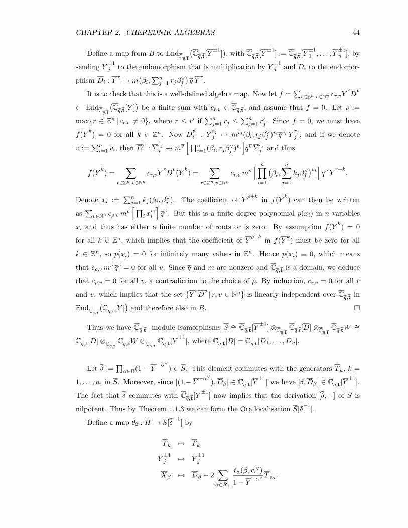
CHAPTER 2. CHEREDNIK ALGEBRAS 44
Define a map from B to EndCq,t
(Cq,t[Y
±1]), with Cq,t[Y
±1] := Cq,t[Y±11 , . . . , Y
±1n ], by
sending Y ±1j to the endomorphism that is multiplication by Y ±1
j and Di to the endomor-
phism Di : Y r 7→ m(βi,
∑nj=1 rjβ
∨j
)q Y
r.
It is to check that this is a well-defined algebra map. Now let f =∑
r∈Zn,v∈Nn cr,vYrDv
∈ EndCq,t
(Cq,t[Y ]
)be a finite sum with cr,v ∈ Cq,t, and assume that f = 0. Let ρ :=
maxr ∈ Zn | cr,v 6= 0, where r ≤ r′ if∑n
j=1 rj ≤∑n
j=1 r′j . Since f = 0, we must have
f(Y k) = 0 for all k ∈ Zn. Now Dvi
i : Y rjj 7→ mvi(βi, rjβ∨j )viqvi Y
rjj , and if we denote
v :=∑n
i=1 vi, then Dv : Y rjj 7→ mv
[ ∏ni=1(βi, rjβ
∨j )vi
]qv Y
rjj and thus
f(Y k) =∑
r∈Zn,v∈Nn
cr,vYrDv(Y k) =
∑r∈Zn,v∈Nn
cr,vmv[ n∏i=1
(βi,
n∑j=1
kjβ∨j
)vi]qv Y
r+k.
Denote xi :=∑n
j=1 kj(βi, β∨j ). The coefficient of Y ρ+k in f(Y k) can then be written
as∑
v∈Nn cρ,vmv[ ∏
i xvii
]qv. But this is a finite degree polynomial p(xi) in n variables
xi and thus has either a finite number of roots or is zero. By assumption f(Y k) = 0
for all k ∈ Zn, which implies that the coefficient of Y ρ+k in f(Y k) must be zero for all
k ∈ Zn, so p(xi) = 0 for infinitely many values in Zn. Hence p(xi) ≡ 0, which means
that cρ,vmv qv = 0 for all v. Since q and m are nonzero and Cq,t is a domain, we deduce
that cρ,v = 0 for all v, a contradiction to the choice of ρ. By induction, cr,v = 0 for all r
and v, which implies that the set Y rDv | r, v ∈ Nn is linearly independent over Cq,t in
EndCq,t
(Cq,t[Y ]
)and therefore also in B.
Thus we have Cq,t -module isomorphisms S ∼= Cq,t[Y±1] ⊗Cq,t
Cq,t[D] ⊗Cq,tCq,tW
∼=
Cq,t[D]⊗Cq,tCq,tW ⊗Cq,t
Cq,t[Y±1], where Cq,t[D] = Cq,t[D1, . . . , Dn].
Let δ :=∏α∈R(1 − Y
−α∨) ∈ S. This element commutes with the generators T k, k =
1, . . . , n, in S. Moreover, since [(1− Y−α∨), Dβ] ∈ Cq,t[Y
±1] we have [δ,Dβ] ∈ Cq,t[Y±1].
The fact that δ commutes with Cq,t[Y±1] now implies that the derivation [δ,−] of S is
nilpotent. Thus by Theorem 1.1.3 we can form the Ore localisation S[δ−1].
Define a map θ2 : H → S[δ−1] by
T k 7→ T k
Y±1j 7→ Y
±1j
Xβ 7→ Dβ − 2∑α∈R+
tα(β, α∨)
1− Y−α∨ T sα .
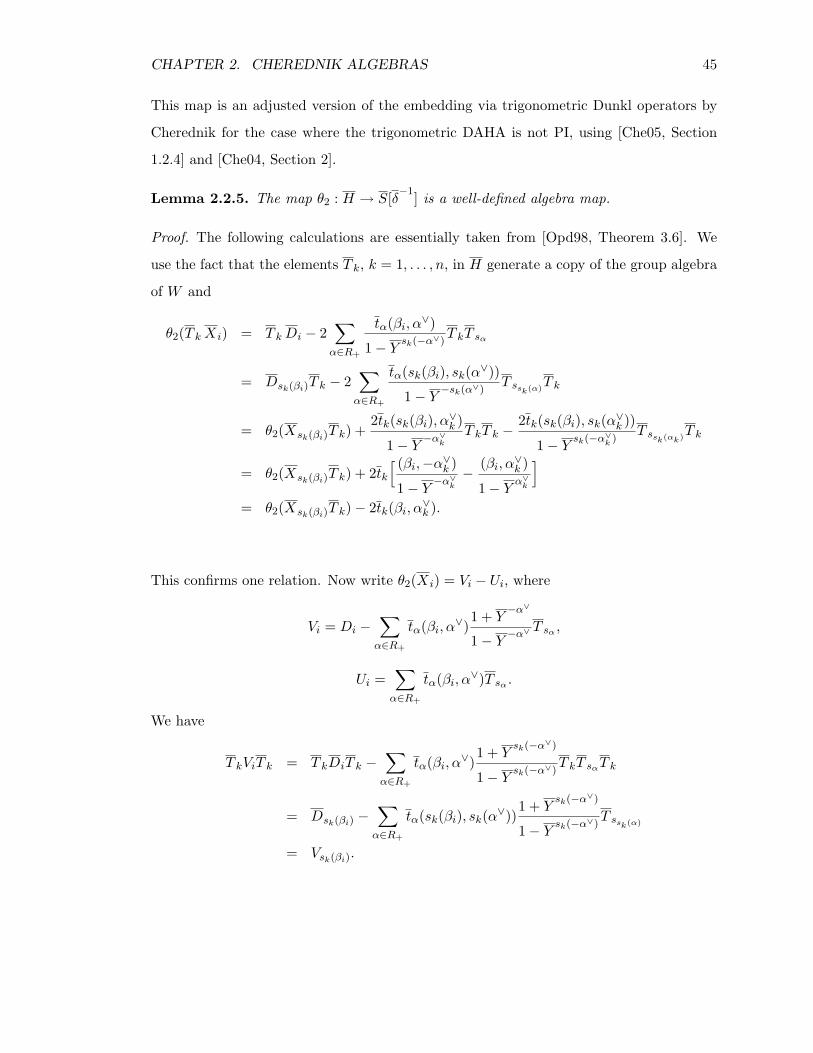
CHAPTER 2. CHEREDNIK ALGEBRAS 45
This map is an adjusted version of the embedding via trigonometric Dunkl operators by
Cherednik for the case where the trigonometric DAHA is not PI, using [Che05, Section
1.2.4] and [Che04, Section 2].
Lemma 2.2.5. The map θ2 : H → S[δ−1] is a well-defined algebra map.
Proof. The following calculations are essentially taken from [Opd98, Theorem 3.6]. We
use the fact that the elements T k, k = 1, . . . , n, in H generate a copy of the group algebra
of W and
θ2(T kXi) = T kDi − 2∑α∈R+
tα(βi, α∨)
1− Ysk(−α∨)
T kT sα
= Dsk(βi)T k − 2∑α∈R+
tα(sk(βi), sk(α∨))
1− Y−sk(α∨)
T ssk(α)T k
= θ2(Xsk(βi)T k) +2tk(sk(βi), α∨k )
1− Y−α∨k
T kT k −2tk(sk(βi), sk(α∨k ))
1− Ysk(−α∨k )
T ssk(αk)T k
= θ2(Xsk(βi)T k) + 2tk[ (βi,−α∨k )
1− Y−α∨k
−(βi, α∨k )
1− Yα∨k
]= θ2(Xsk(βi)T k)− 2tk(βi, α∨k ).
This confirms one relation. Now write θ2(Xi) = Vi − Ui, where
Vi = Di −∑α∈R+
tα(βi, α∨)1 + Y
−α∨
1− Y−α∨ T sα ,
Ui =∑α∈R+
tα(βi, α∨)T sα .
We have
T kViT k = T kDiT k −∑α∈R+
tα(βi, α∨)1 + Y
sk(−α∨)
1− Ysk(−α∨)
T kT sαT k
= Dsk(βi) −∑α∈R+
tα(sk(βi), sk(α∨))1 + Y
sk(−α∨)
1− Ysk(−α∨)
T ssk(α)
= Vsk(βi).
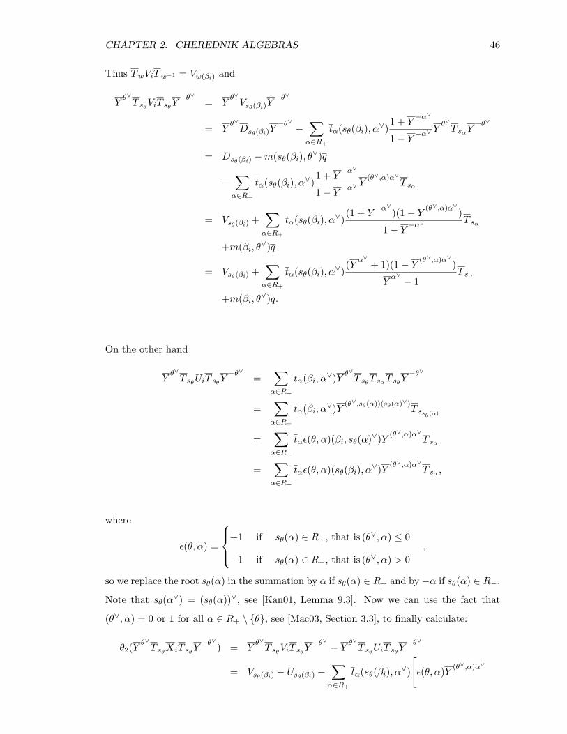
CHAPTER 2. CHEREDNIK ALGEBRAS 46
Thus TwViTw−1 = Vw(βi) and
Yθ∨T sθ
ViT sθY−θ∨ = Y
θ∨Vsθ(βi)Y
−θ∨
= Yθ∨Dsθ(βi)Y
−θ∨ −∑α∈R+
tα(sθ(βi), α∨)1 + Y
−α∨
1− Y−α∨ Y
θ∨T sαY
−θ∨
= Dsθ(βi) −m(sθ(βi), θ∨)q
−∑α∈R+
tα(sθ(βi), α∨)1 + Y
−α∨
1− Y−α∨ Y
(θ∨,α)α∨T sα
= Vsθ(βi) +∑α∈R+
tα(sθ(βi), α∨)(1 + Y
−α∨)(1− Y(θ∨,α)α∨)
1− Y−α∨ T sα
+m(βi, θ∨)q
= Vsθ(βi) +∑α∈R+
tα(sθ(βi), α∨)(Y α∨ + 1)(1− Y
(θ∨,α)α∨)
Yα∨ − 1
T sα
+m(βi, θ∨)q.
On the other hand
Yθ∨T sθ
UiT sθY−θ∨ =
∑α∈R+
tα(βi, α∨)Yθ∨T sθ
T sαT sθY−θ∨
=∑α∈R+
tα(βi, α∨)Y(θ∨,sθ(α))(sθ(α)∨)
T ssθ(α)
=∑α∈R+
tαε(θ, α)(βi, sθ(α)∨)Y (θ∨,α)α∨T sα
=∑α∈R+
tαε(θ, α)(sθ(βi), α∨)Y(θ∨,α)α∨
T sα ,
where
ε(θ, α) =
+1 if sθ(α) ∈ R+, that is (θ∨, α) ≤ 0
−1 if sθ(α) ∈ R−, that is (θ∨, α) > 0,
so we replace the root sθ(α) in the summation by α if sθ(α) ∈ R+ and by −α if sθ(α) ∈ R−.
Note that sθ(α∨) = (sθ(α))∨, see [Kan01, Lemma 9.3]. Now we can use the fact that
(θ∨, α) = 0 or 1 for all α ∈ R+ \ θ, see [Mac03, Section 3.3], to finally calculate:
θ2(Yθ∨T sθ
XiT sθY−θ∨) = Y
θ∨T sθ
ViT sθY−θ∨ − Y
θ∨T sθ
UiT sθY−θ∨
= Vsθ(βi) − Usθ(βi) −∑α∈R+
tα(sθ(βi), α∨)
[ε(θ, α)Y (θ∨,α)α∨
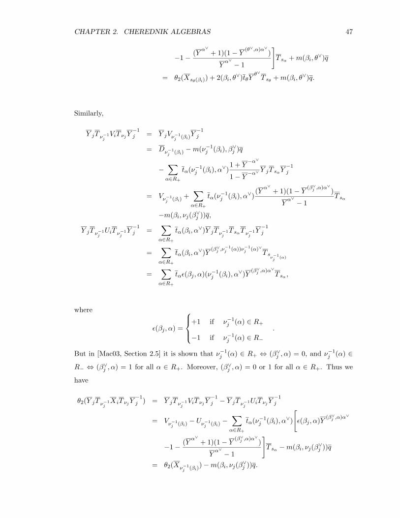
CHAPTER 2. CHEREDNIK ALGEBRAS 47
−1− (Y α∨ + 1)(1− Y(θ∨,α)α∨)
Yα∨ − 1
]T sα +m(βi, θ∨)q
= θ2(Xsθ(βi)) + 2(βi, θ∨)tθYθ∨T sθ
+m(βi, θ∨)q.
Similarly,
Y jT ν−1jViT νjY
−1j = Y jVν−1
j (βi)Y−1j
= Dν−1j (βi)
−m(ν−1j (βi), β∨j )q
−∑α∈R+
tα(ν−1j (βi), α∨)
1 + Y−α∨
1− Y−α∨ Y jT sαY
−1j
= Vν−1j (βi)
+∑α∈R+
tα(ν−1j (βi), α∨)
(Y α∨ + 1)(1− Y(β∨j ,α)α∨)
Yα∨ − 1
T sα
−m(βi, νj(β∨j ))q,
Y jT ν−1jUiT ν−1
jY−1j =
∑α∈R+
tα(βi, α∨)Y jT ν−1jT sαT ν−1
jY−1j
=∑α∈R+
tα(βi, α∨)Y(β∨j ,ν
−1j (α))ν−1
j (α)∨T s
ν−1j
(α)
=∑α∈R+
tαε(βj , α)(ν−1j (βi), α∨)Y
(β∨j ,α)α∨T sα ,
where
ε(βj , α) =
+1 if ν−1
j (α) ∈ R+
−1 if ν−1j (α) ∈ R−
.
But in [Mac03, Section 2.5] it is shown that ν−1j (α) ∈ R+ ⇔ (β∨j , α) = 0, and ν−1
j (α) ∈
R− ⇔ (β∨j , α) = 1 for all α ∈ R+. Moreover, (β∨j , α) = 0 or 1 for all α ∈ R+. Thus we
have
θ2(Y jT ν−1jXiT νjY
−1j ) = Y jT ν−1
jViT νjY
−1j − Y jT ν−1
jUiT νjY
−1j
= Vν−1j (βi)
− Uν−1j (βi)
−∑α∈R+
tα(ν−1j (βi), α∨)
[ε(βj , α)Y (β∨j ,α)α∨
−1− (Y α∨ + 1)(1− Y(β∨j ,α)α∨)
Yα∨ − 1
]T sα −m(βi, νj(β∨j ))q
= θ2(Xν−1j (βi)
)−m(βi, νj(β∨j ))q.
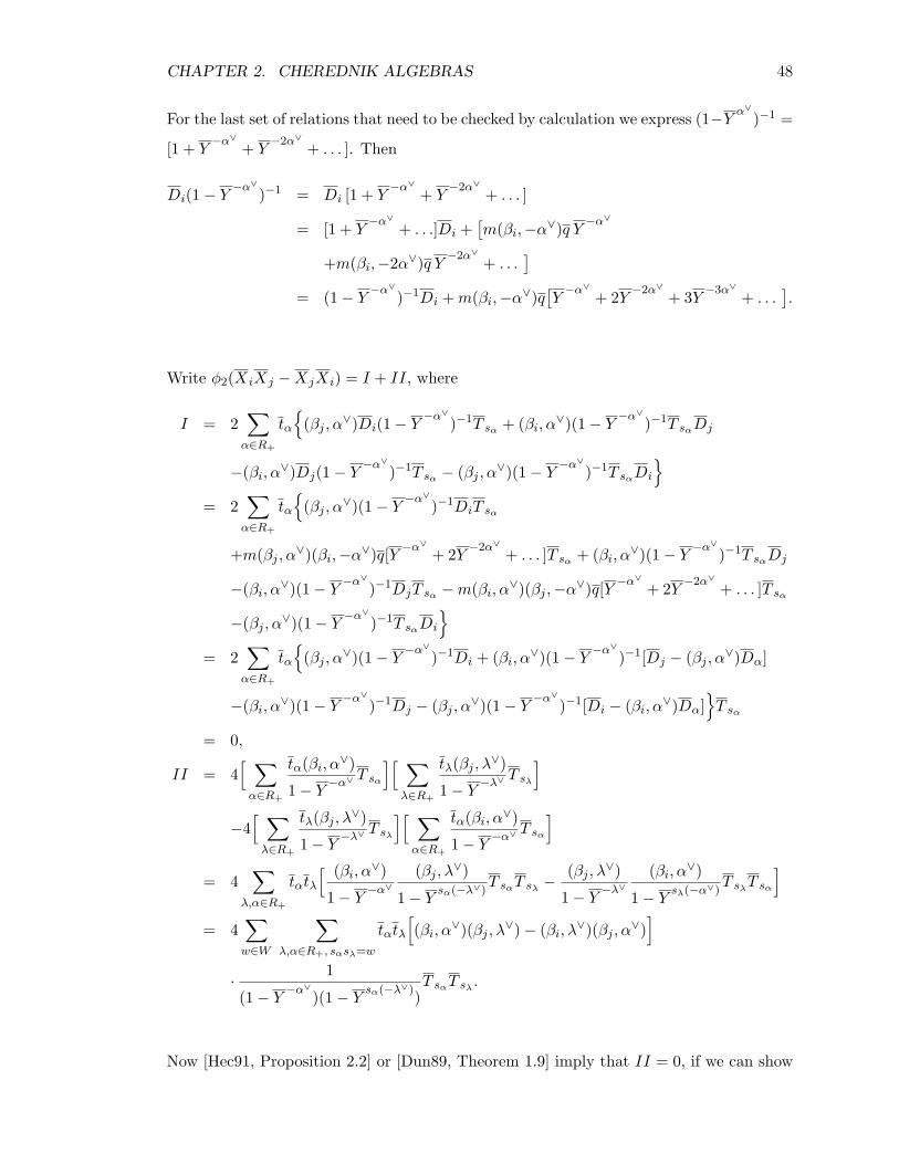
CHAPTER 2. CHEREDNIK ALGEBRAS 48
For the last set of relations that need to be checked by calculation we express (1−Y α∨)−1 =
[1 + Y−α∨ + Y
−2α∨ + . . . ]. Then
Di(1− Y−α∨)−1 = Di [1 + Y
−α∨ + Y−2α∨ + . . . ]
= [1 + Y−α∨ + . . .]Di +
[m(βi,−α∨)q Y
−α∨
+m(βi,−2α∨)q Y −2α∨ + . . .]
= (1− Y−α∨)−1Di +m(βi,−α∨)q
[Y−α∨ + 2Y −2α∨ + 3Y −3α∨ + . . .
].
Write φ2(XiXj −XjXi) = I + II, where
I = 2∑α∈R+
tα
(βj , α∨)Di(1− Y
−α∨)−1T sα + (βi, α∨)(1− Y−α∨)−1T sαDj
−(βi, α∨)Dj(1− Y−α∨)−1T sα − (βj , α∨)(1− Y
−α∨)−1T sαDi
= 2
∑α∈R+
tα
(βj , α∨)(1− Y
−α∨)−1DiT sα
+m(βj , α∨)(βi,−α∨)q[Y−α∨ + 2Y −2α∨ + . . . ]T sα + (βi, α∨)(1− Y
−α∨)−1T sαDj
−(βi, α∨)(1− Y−α∨)−1DjT sα −m(βi, α∨)(βj ,−α∨)q[Y
−α∨ + 2Y −2α∨ + . . . ]T sα
−(βj , α∨)(1− Y−α∨)−1T sαDi
= 2
∑α∈R+
tα
(βj , α∨)(1− Y
−α∨)−1Di + (βi, α∨)(1− Y−α∨)−1[Dj − (βj , α∨)Dα]
−(βi, α∨)(1− Y−α∨)−1Dj − (βj , α∨)(1− Y
−α∨)−1[Di − (βi, α∨)Dα]T sα
= 0,
II = 4[ ∑α∈R+
tα(βi, α∨)
1− Y−α∨ T sα
][ ∑λ∈R+
tλ(βj , λ∨)
1− Y−λ∨ T sλ
]−4
[ ∑λ∈R+
tλ(βj , λ∨)
1− Y−λ∨ T sλ
][ ∑α∈R+
tα(βi, α∨)
1− Y−α∨ T sα
]= 4
∑λ,α∈R+
tαtλ
[ (βi, α∨)
1− Y−α∨
(βj , λ∨)
1− Ysα(−λ∨)
T sαT sλ− (βj , λ∨)
1− Y−λ∨
(βi, α∨)
1− Ysλ(−α∨)
T sλT sα
]= 4
∑w∈W
∑λ,α∈R+, sαsλ=w
tαtλ
[(βi, α∨)(βj , λ∨)− (βi, λ∨)(βj , α∨)
]· 1
(1− Y−α∨)(1− Y
sα(−λ∨))T sαT sλ
.
Now [Hec91, Proposition 2.2] or [Dun89, Theorem 1.9] imply that II = 0, if we can show
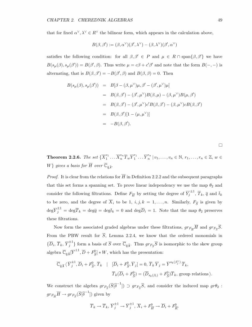
CHAPTER 2. CHEREDNIK ALGEBRAS 49
that for fixed α∨, λ∨ ∈ R∨ the bilinear form, which appears in the calculation above,
B(β, β′) := (β, α∨)(β′, λ∨)− (β, λ∨)(β′, α∨)
satisfies the following condition: for all β, β′ ∈ P and µ ∈ R ∩ spanβ, β′ we have
B(sµ(β), sµ(β′)) = B(β′, β). Thus write µ = cβ + c′β′ and note that the form B(−,−) is
alternating, that is B(β, β′) = −B(β′, β) and B(β, β) = 0. Then
B(sµ(β), sµ(β′)) = B[β − (β, µ∨)µ, β′ − (β′, µ∨)µ]
= B(β, β′)− (β′, µ∨)B(β, µ)− (β, µ∨)B(µ, β′)
= B(β, β′)− (β′, µ∨)c′B(β, β′)− (β, µ∨)cB(β, β′)
= B(β, β′)[1− (µ, µ∨)]
= −B(β, β′).
Theorem 2.2.6. The set Xv11 . . . X
vn
n TwYr11 . . . Y
rnn | v1, . . . , vn ∈ N, r1, . . . , rn ∈ Z, w ∈
W gives a basis for H over Cq,t.
Proof. It is clear from the relations forH in Definition 2.2.2 and the subsequent paragraphs
that this set forms a spanning set. To prove linear independency we use the map θ2 and
consider the following filtrations. Define FH by setting the degree of Yj±1, T k, q and tk
to be zero, and the degree of Xi to be 1, i, j, k = 1, . . . , n. Similarly, FS is given by
degY ±1j = degT k = degq = degtk = 0 and degDi = 1. Note that the map θ2 preserves
these filtrations.
Now form the associated graded algebras under these filtrations, grFHH and grFS
S.
From the PBW result for S, Lemma 2.2.4, we know that the ordered monomials in
Di, T k, Y±1j form a basis of S over Cq,t. Thus grFS
S is isomorphic to the skew group
algebra Cq,t[Y±1, D + F0
S] ∗W , which has the presentation:
Cq,t 〈Y±1j , Di + F0
S, T k | [Di + F0
S, Y j ] = 0, T k Y j = Y
sk(β∨j )T k,
T k(Di + F0S) = (Dsk(βi) + F0
S)T k, group relations 〉.
We construct the algebra grFS(S[δ−1]) ⊃ grFS
S, and consider the induced map grθ2 :
grFHH → grFS
(S[δ−1]) given by
T k → T k, Y±1j → Y
±1j , Xi + F0
H→ Di + F0
R.
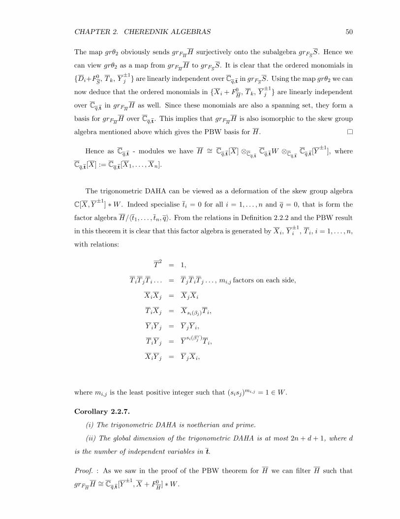
CHAPTER 2. CHEREDNIK ALGEBRAS 50
The map grθ2 obviously sends grFHH surjectively onto the subalgebra grFS
S. Hence we
can view grθ2 as a map from grFHH to grFS
S. It is clear that the ordered monomials in
Di+F0S, T k, Y
±1j are linearly independent over Cq,t in grFS
S. Using the map grθ2 we can
now deduce that the ordered monomials in Xi + F0H, T k, Y
±1j are linearly independent
over Cq,t in grFHH as well. Since these monomials are also a spanning set, they form a
basis for grFHH over Cq,t. This implies that grFH
H is also isomorphic to the skew group
algebra mentioned above which gives the PBW basis for H.
Hence as Cq,t - modules we have H ∼= Cq,t[X] ⊗Cq,tCq,tW ⊗Cq,t
Cq,t[Y±1], where
Cq,t[X] := Cq,t[X1, . . . , Xn].
The trigonometric DAHA can be viewed as a deformation of the skew group algebra
C[X,Y ±1] ∗W . Indeed specialise ti = 0 for all i = 1, . . . , n and q = 0, that is form the
factor algebra H/〈t1, . . . , tn, q〉. From the relations in Definition 2.2.2 and the PBW result
in this theorem it is clear that this factor algebra is generated by Xi, Y±1i , T i, i = 1, . . . , n,
with relations:
T2 = 1,
T iT jT i . . . = T jT iT j . . . , mi,j factors on each side,
XiXj = XjXi
T iXj = Xsi(βj)T i,
Y iY j = Y jY i,
T iY j = Ysi(β
∨j )T i,
XiY j = Y jXi,
where mi,j is the least positive integer such that (sisj)mi,j = 1 ∈W .
Corollary 2.2.7.
(i) The trigonometric DAHA is noetherian and prime.
(ii) The global dimension of the trigonometric DAHA is at most 2n + d + 1, where d
is the number of independent variables in t.
Proof. : As we saw in the proof of the PBW theorem for H we can filter H such that
grFHH ∼= Cq,t[Y
±1, X + F0
H] ∗W .
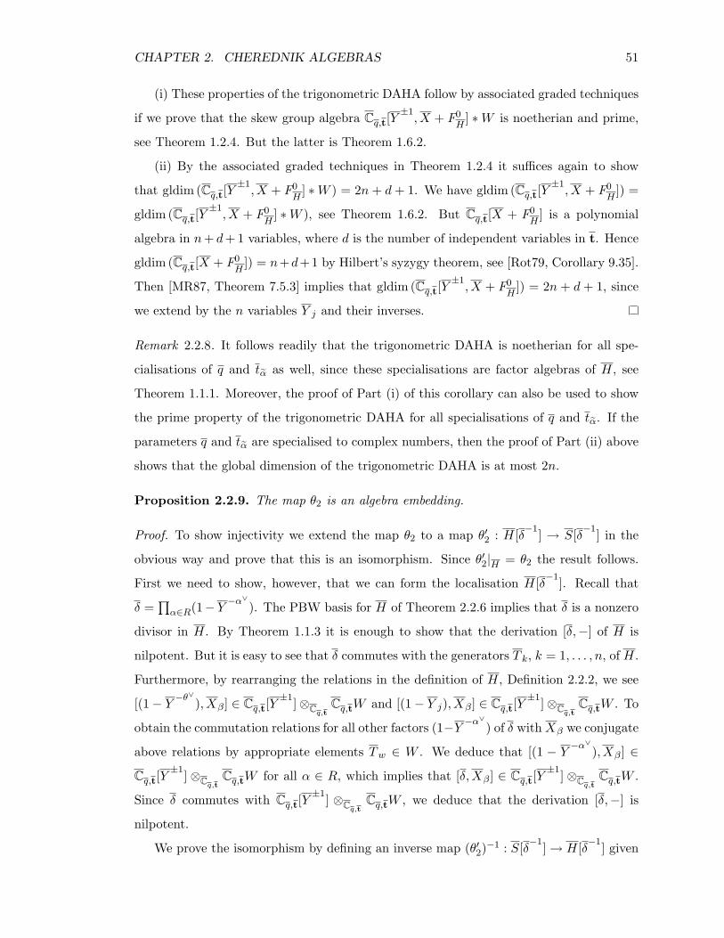
CHAPTER 2. CHEREDNIK ALGEBRAS 51
(i) These properties of the trigonometric DAHA follow by associated graded techniques
if we prove that the skew group algebra Cq,t[Y±1, X + F0
H] ∗W is noetherian and prime,
see Theorem 1.2.4. But the latter is Theorem 1.6.2.
(ii) By the associated graded techniques in Theorem 1.2.4 it suffices again to show
that gldim (Cq,t[Y±1, X + F0
H] ∗W ) = 2n+ d + 1. We have gldim (Cq,t[Y
±1, X + F0
H]) =
gldim (Cq,t[Y±1, X + F0
H] ∗W ), see Theorem 1.6.2. But Cq,t[X + F0
H] is a polynomial
algebra in n+ d+ 1 variables, where d is the number of independent variables in t. Hence
gldim (Cq,t[X + F0H
]) = n+d+1 by Hilbert’s syzygy theorem, see [Rot79, Corollary 9.35].
Then [MR87, Theorem 7.5.3] implies that gldim (Cq,t[Y±1, X + F0
H]) = 2n + d + 1, since
we extend by the n variables Y j and their inverses.
Remark 2.2.8. It follows readily that the trigonometric DAHA is noetherian for all spe-
cialisations of q and tα as well, since these specialisations are factor algebras of H, see
Theorem 1.1.1. Moreover, the proof of Part (i) of this corollary can also be used to show
the prime property of the trigonometric DAHA for all specialisations of q and tα. If the
parameters q and tα are specialised to complex numbers, then the proof of Part (ii) above
shows that the global dimension of the trigonometric DAHA is at most 2n.
Proposition 2.2.9. The map θ2 is an algebra embedding.
Proof. To show injectivity we extend the map θ2 to a map θ′2 : H[δ−1] → S[δ−1] in the
obvious way and prove that this is an isomorphism. Since θ′2|H = θ2 the result follows.
First we need to show, however, that we can form the localisation H[δ−1]. Recall that
δ =∏α∈R(1−Y −α
∨). The PBW basis for H of Theorem 2.2.6 implies that δ is a nonzero
divisor in H. By Theorem 1.1.3 it is enough to show that the derivation [δ,−] of H is
nilpotent. But it is easy to see that δ commutes with the generators T k, k = 1, . . . , n, of H.
Furthermore, by rearranging the relations in the definition of H, Definition 2.2.2, we see
[(1− Y −θ∨), Xβ] ∈ Cq,t[Y
±1]⊗Cq,tCq,tW and [(1− Y j), Xβ ] ∈ Cq,t[Y
±1]⊗Cq,tCq,tW . To
obtain the commutation relations for all other factors (1−Y −α∨) of δ withXβ we conjugate
above relations by appropriate elements Tw ∈ W . We deduce that [(1 − Y−α∨), Xβ] ∈
Cq,t[Y±1] ⊗Cq,t
Cq,tW for all α ∈ R, which implies that [δ,Xβ ] ∈ Cq,t[Y±1] ⊗Cq,t
Cq,tW .
Since δ commutes with Cq,t[Y±1] ⊗Cq,t
Cq,tW , we deduce that the derivation [δ,−] is
nilpotent.
We prove the isomorphism by defining an inverse map (θ′2)−1 : S[δ−1] → H[δ−1] given
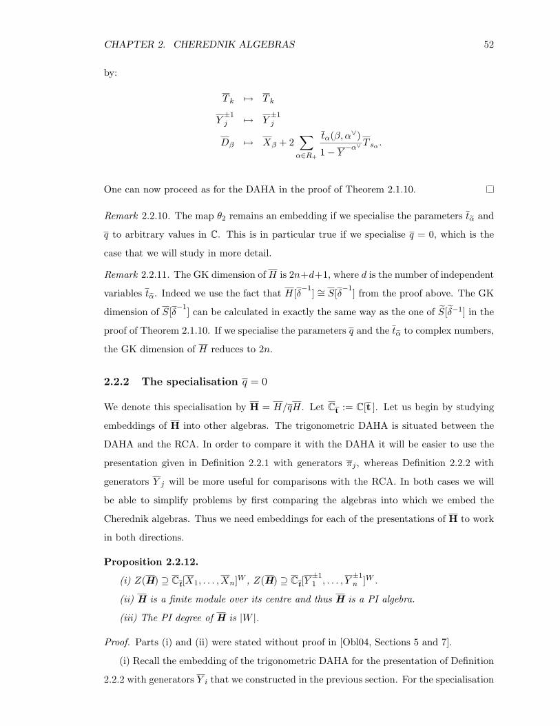
CHAPTER 2. CHEREDNIK ALGEBRAS 52
by:
T k 7→ T k
Y±1j 7→ Y
±1j
Dβ 7→ Xβ + 2∑α∈R+
tα(β, α∨)
1− Y−α∨ T sα .
One can now proceed as for the DAHA in the proof of Theorem 2.1.10.
Remark 2.2.10. The map θ2 remains an embedding if we specialise the parameters tα and
q to arbitrary values in C. This is in particular true if we specialise q = 0, which is the
case that we will study in more detail.
Remark 2.2.11. The GK dimension of H is 2n+d+1, where d is the number of independent
variables tα. Indeed we use the fact that H[δ−1] ∼= S[δ−1] from the proof above. The GK
dimension of S[δ−1] can be calculated in exactly the same way as the one of S[δ−1] in the
proof of Theorem 2.1.10. If we specialise the parameters q and the tα to complex numbers,
the GK dimension of H reduces to 2n.
2.2.2 The specialisation q = 0
We denote this specialisation by H = H/qH. Let Ct := C[t ]. Let us begin by studying
embeddings of H into other algebras. The trigonometric DAHA is situated between the
DAHA and the RCA. In order to compare it with the DAHA it will be easier to use the
presentation given in Definition 2.2.1 with generators πj , whereas Definition 2.2.2 with
generators Y j will be more useful for comparisons with the RCA. In both cases we will
be able to simplify problems by first comparing the algebras into which we embed the
Cherednik algebras. Thus we need embeddings for each of the presentations of H to work
in both directions.
Proposition 2.2.12.
(i) Z(H) ⊇ Ct[X1, . . . , Xn]W , Z(H) ⊇ Ct[Y±11 , . . . , Y
±1n ]W .
(ii) H is a finite module over its centre and thus H is a PI algebra.
(iii) The PI degree of H is |W |.
Proof. Parts (i) and (ii) were stated without proof in [Obl04, Sections 5 and 7].
(i) Recall the embedding of the trigonometric DAHA for the presentation of Definition
2.2.2 with generators Y i that we constructed in the previous section. For the specialisation
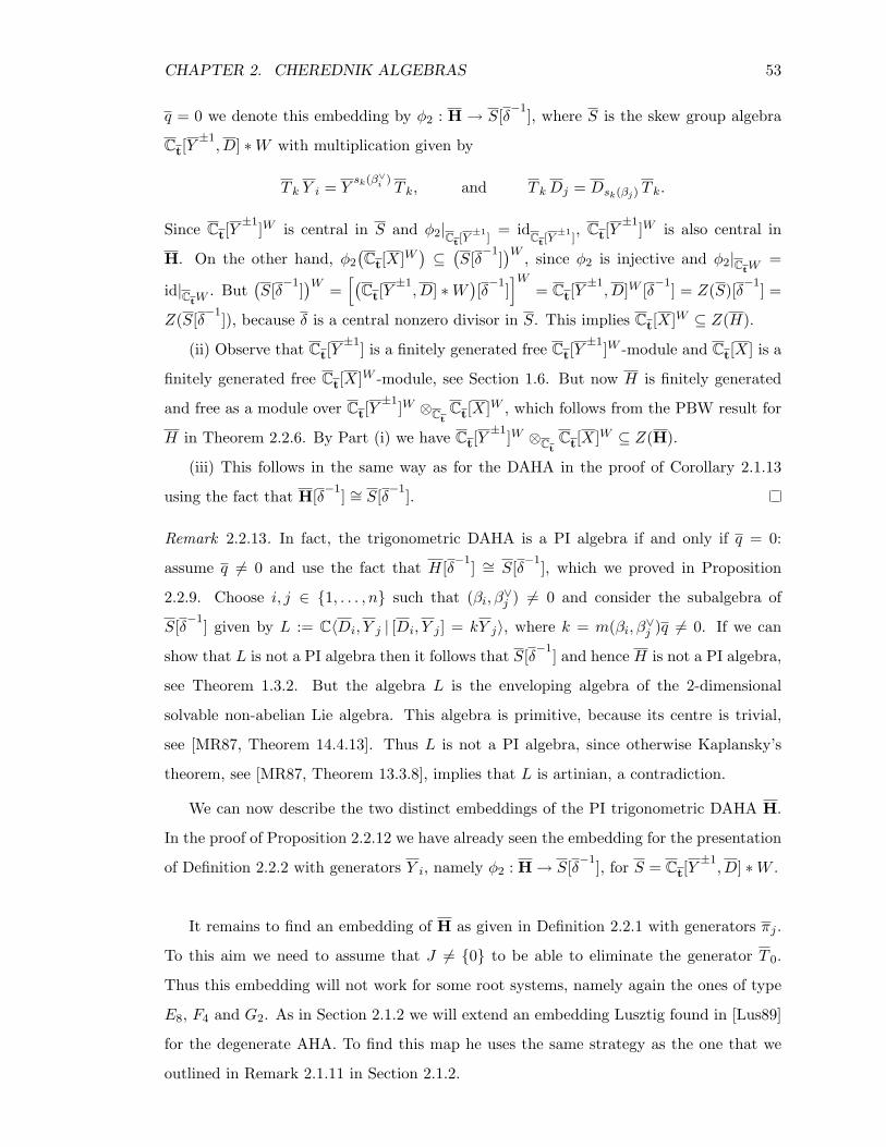
CHAPTER 2. CHEREDNIK ALGEBRAS 53
q = 0 we denote this embedding by φ2 : H → S[δ−1], where S is the skew group algebra
Ct[Y±1, D] ∗W with multiplication given by
T k Y i = Ysk(β∨i )
T k, and T kDj = Dsk(βj) T k.
Since Ct[Y±1]W is central in S and φ2|Ct[Y
±1]
= idCt[Y±1
], Ct[Y
±1]W is also central in
H. On the other hand, φ2
(Ct[X]W
)⊆
(S[δ−1]
)W , since φ2 is injective and φ2|CtW=
id|CtW. But
(S[δ−1]
)W =[(
Ct[Y±1, D] ∗W
)[δ−1]
]W= Ct[Y
±1, D]W [δ−1] = Z(S)[δ−1] =
Z(S[δ−1]), because δ is a central nonzero divisor in S. This implies Ct[X]W ⊆ Z(H).
(ii) Observe that Ct[Y±1] is a finitely generated free Ct[Y
±1]W -module and Ct[X] is a
finitely generated free Ct[X]W -module, see Section 1.6. But now H is finitely generated
and free as a module over Ct[Y±1]W ⊗Ct
Ct[X]W , which follows from the PBW result for
H in Theorem 2.2.6. By Part (i) we have Ct[Y±1]W ⊗Ct
Ct[X]W ⊆ Z(H).
(iii) This follows in the same way as for the DAHA in the proof of Corollary 2.1.13
using the fact that H[δ−1] ∼= S[δ−1].
Remark 2.2.13. In fact, the trigonometric DAHA is a PI algebra if and only if q = 0:
assume q 6= 0 and use the fact that H[δ−1] ∼= S[δ−1], which we proved in Proposition
2.2.9. Choose i, j ∈ 1, . . . , n such that (βi, β∨j ) 6= 0 and consider the subalgebra of
S[δ−1] given by L := C〈Di, Y j | [Di, Y j ] = kY j〉, where k = m(βi, β∨j )q 6= 0. If we can
show that L is not a PI algebra then it follows that S[δ−1] and hence H is not a PI algebra,
see Theorem 1.3.2. But the algebra L is the enveloping algebra of the 2-dimensional
solvable non-abelian Lie algebra. This algebra is primitive, because its centre is trivial,
see [MR87, Theorem 14.4.13]. Thus L is not a PI algebra, since otherwise Kaplansky’s
theorem, see [MR87, Theorem 13.3.8], implies that L is artinian, a contradiction.
We can now describe the two distinct embeddings of the PI trigonometric DAHA H.
In the proof of Proposition 2.2.12 we have already seen the embedding for the presentation
of Definition 2.2.2 with generators Y i, namely φ2 : H → S[δ−1], for S = Ct[Y±1, D] ∗W .
It remains to find an embedding of H as given in Definition 2.2.1 with generators πj .
To this aim we need to assume that J 6= 0 to be able to eliminate the generator T 0.
Thus this embedding will not work for some root systems, namely again the ones of type
E8, F4 and G2. As in Section 2.1.2 we will extend an embedding Lusztig found in [Lus89]
for the degenerate AHA. To find this map he uses the same strategy as the one that we
outlined in Remark 2.1.11 in Section 2.1.2.
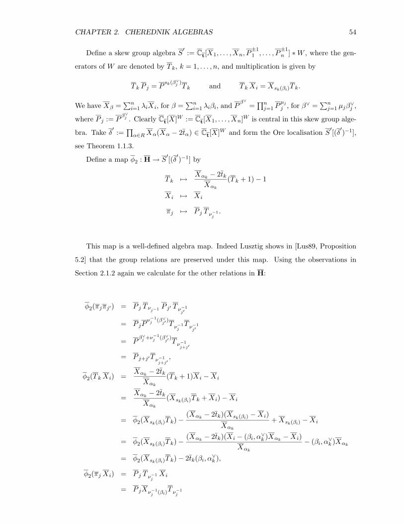
CHAPTER 2. CHEREDNIK ALGEBRAS 54
Define a skew group algebra S′ := Ct[X1, . . . , Xn, P±11 , . . . , P
±1n ] ∗W , where the gen-
erators of W are denoted by T k, k = 1, . . . , n, and multiplication is given by
T k P j = Psk(β∨j )
T k and T kXi = Xsk(βi)T k.
We have Xβ =∑n
i=1 λiXi, for β =∑n
i=1 λiβi, and P β∨
=∏nj=1 P
µj
j , for β∨ =∑n
j=1 µjβ∨j ,
where P j := Pβ∨j . Clearly Ct[X]W := Ct[X1, . . . , Xn]W is central in this skew group alge-
bra. Take δ′ :=∏α∈RXα(Xα − 2tα) ∈ Ct[X]W and form the Ore localisation S
′[(δ′)−1],
see Theorem 1.1.3.
Define a map φ2 : H → S′[(δ′)−1] by
T k 7→ Xαk− 2tk
Xαk
(T k + 1)− 1
Xi 7→ Xi
πj 7→ P j T ν−1j.
This map is a well-defined algebra map. Indeed Lusztig shows in [Lus89, Proposition
5.2] that the group relations are preserved under this map. Using the observations in
Section 2.1.2 again we calculate for the other relations in H:
φ2(πjπj′) = P j T νj−1 P j′ T ν−1j′
= P jPν−1
j (β∨j′ )T ν−1
jT ν−1
j′
= Pβ∨j +ν−1
j (β∨j′ )T ν−1
j+j′
= P j+j′T ν−1j+j′
,
φ2(T kXi) =Xαk
− 2tkXαk
(T k + 1)Xi −Xi
=Xαk
− 2tkXαk
(Xsk(βi)T k +Xi)−Xi
= φ2(Xsk(βi)T k)−(Xαk
− 2tk)(Xsk(βi) −Xi)
Xαk
+Xsk(βi) −Xi
= φ2(Xsk(βi)T k)−(Xαk
− 2tk)(Xi − (βi, α∨k )Xαk−Xi)
Xαk
− (βi, α∨k )Xαk
= φ2(Xsk(βi)T k)− 2tk(βi, α∨k ),
φ2(πj Xi) = P j T ν−1jXi
= P jXν−1j (βi)
T ν−1j
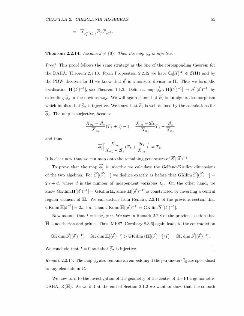
CHAPTER 2. CHEREDNIK ALGEBRAS 55
= Xν−1j (βi)
P j T ν−1j.
Theorem 2.2.14. Assume J 6= 0. Then the map φ2 is injective.
Proof. This proof follows the same strategy as the one of the corresponding theorem for
the DAHA, Theorem 2.1.10. From Proposition 2.2.12 we have Ct[X]W ∈ Z(H) and by
the PBW theorem for H we know that δ′ is a nonzero divisor in H. Thus we form the
localisation H[(δ′)−1], see Theorem 1.1.3. Define a map φ′2 : H[(δ′)−1] → S
′[(δ′)−1] by
extending φ2 in the obvious way. We will again show that φ′2 is an algebra isomorphism
which implies that φ2 is injective. We know that φ′2 is well-defined by the calculations for
φ2. The map is surjective, because:
Xαk− 2tk
Xαk
(T k + 1)− 1 =Xαk
− 2tkXαk
T k −2tkXαk
and thus
φ′2
[ Xαk
Xαk− 2tk
(T k +2tkXαk
)]
= T k.
It is clear now that we can map onto the remaining generators of S′[(δ′)−1].
To prove that the map φ′2 is injective we calculate the Gelfand-Kirillov dimensions
of the two algebras. For S′[(δ′)−1] we deduce exactly as before that GKdimS′[(δ′)−1] =
2n + d, where d is the number of independent variables tα. On the other hand, we
know GKdimH[(δ′)−1] = GKdimH, since H[(δ′)−1] is constructed by inverting a central
regular element of H. We can deduce from Remark 2.2.11 of the previous section that
GKdimH[δ−1] = 2n+ d. Thus GKdimH[(δ′)−1] = GKdimS′[(δ′)−1].
Now assume that I = kerφ′2 6= 0. We saw in Remark 2.2.8 of the previous section that
H is noetherian and prime. Thus [MR87, Corollary 8.3.6] again leads to the contradiction
GKdimS′[(δ′)−1] = GKdimH[(δ′)−1] > GKdim
(H[(δ′)−1]/I
)= GK dimS
′[(δ′)−1].
We conclude that I = 0 and that φ′2 is injective.
Remark 2.2.15. The map φ2 also remains an embedding if the parameters tα are specialised
to any elements in C.
We now turn to the investigation of the geometry of the centre of the PI trigonometric
DAHA, Z(H). As we did at the end of Section 2.1.2 we want to show that the smooth
CHAPTER 2. CHEREDNIK ALGEBRAS 56
points in Z(H) are precisely the Azumaya points of H. To this aim we again construct
the spherical subalgebra of H. Namely, let e ∈ CW be the symmetrizing idempotent
e =1|W |
∑w∈W
Tw
and eHe the spherical subalgebra. The space He has an obvious right eHe-module struc-
ture and in analogy to Proposition 2.1.14 we have the following result:
Proposition 2.2.16. [Obl04, Theorem 5.1, Theorem 7.1]
(i) eHe is a domain.
(ii) The right eHe-module He is finitely generated.
(iii) There is an algebra isomorphism H ∼= EndeHe(He).
(iv) Z(H) ∼= eHe.
(v) He is a Cohen-Macaulay module over eHe.
Proof. Oblomkov’s work only contains a rough outline of a proof for statements (i)-(iv).
We provide the details of an alternative proof.
The key ingredient is the filtration on H described in the proof of Theorem 2.2.6, such
that grFHH ∼= Ct[Y
±1, X+F0
H] ∗W . This filtration induces by intersection a filtration on
both eHe and He. It is easy to see that
grFHeHe = e
(grFH
H)e ∼= e
(Ct[Y
±1, X + F0
H] ∗W
)e ∼= Ct[Y
±1, X + F0
H]W .
The inverse of the last isomorphism is given by the mapping p 7→ pe. Similarly, grFHHe ∼=
Ct[Y±1, X + F0
H]. Therefore, one can use the proofs for analogous statements in [EG02]:
(i), (ii) and (iii) follow as in the proof of [EG02, Theorem 1.5 (i), (ii), (iii)].
Part (iv) follows as in the proof of [EG02, Theorem 3.1]. The fact that eHe is commu-
tative can be deduced easily using the embedding φ2 : H → S[δ−1], S = Ct[Y±1, D] ∗W ,
since φ2|CtW= id|CtW
, and e(S[δ−1]
)e = (e S e)[δ−1] ∼= Ct[Y
±1, D]W [δ−1] as δ is a central
regular element in S.
(v) The proof is exactly the same as the one by [Obl04, Theorem 5.1] for the DAHA and
we describe it here for completeness. Denote B := Ct[X]W ⊗CtCt[Y
±1]W ⊆ Z(H) ∼= eHe,
and observe that eHe is finitely generated over B, since H is finitely generated over
B by Proposition 2.2.12. By [BBG97, Theorem 2.1] it now suffices to show that He
is a Cohen-Macaulay module over B. The B-module He is Cohen-Macaulay if for all
maximal ideals mCB the localisations (He)m are Cohen-Macaulay modules over Bm. By
CHAPTER 2. CHEREDNIK ALGEBRAS 57
definition, [Eis95, Definition 21.9], (He)m is a (maximal) Cohen-Macaulay module over
Bm if depth(He)m = dimBm, where dimBm denotes the Krull dimension of Bm. Now
B is a commutative ring with finite global dimension, which can be seen from [MR87,
Theorem 7.5.3]. Therefore, Bm is a local ring with finite global dimension and hence
regular, see Theorems 1.1.5 and 1.4.3. This implies that Bm is itself Cohen-Macaulay and
thus depthBm = dimBm, see [Har77, Theorem II.8.21A]. If we can show that (He)m
is a finitely generated projective Bm-module, then the Auslander-Buchsbaum formula,
c.f [Eis95, Theorem 19.9], implies that depth(He)m = dimBm, and we are done. Let us
prove that He is a projective B-module. It is then easy to see that the same argument
gives that (He)m is a projective Bm-module for all maximal ideals mCB, since localisation
preserves direct sums. Note that He is a finitely generated B-module, since H is a finitely
generated B-module. Moreover, He is a direct summand of H, as H = He ⊕H(1 − e).
But H is a free B-module as we saw in the proof of Part (ii) of Proposition 2.2.12.
Theorem 2.2.17. A point in MaxSpecZ(H) is smooth if and only if it is Azumaya.
Proof. The fact that an Azumaya point is smooth follows if the global dimension of H
is finite, as described in Theorem 1.4.5. Now Corollary 2.2.7 and the subsequent remark
show that gldimH < ∞. For the converse statement we use the previous proposition
and exactly the same proof as for the corresponding result for the DAHA in Theorem
2.1.15.
Remark 2.2.18. Proposition 2.2.16 and Theorem 2.2.17 also hold when the parameters in
t are specialised to complex numbers.
2.3 The rational Cherednik algebra
2.3.1 Definition and first properties
Let t = tα |α ∈ R be indeterminates such that tα = tα′ if sα and sα′ are conjugate in
W . Thus there are one or two independent variables tα depending on whether there are
one or two root lengths in R. Denote Cq,t := C[q, t]. The RCA was defined by Etingof
and Ginzburg in [EG02] as follows.
Definition 2.3.1. [EG02, Section 1, p. 251] The RCA, H, is generated over Cq,t by
CHAPTER 2. CHEREDNIK ALGEBRAS 58
W = 〈T1, . . . , Tn〉, XR := Xα |α ∈ R and YR∨ := Yα∨ |α∨ ∈ R∨ with relations:
XαXα′ = Xα′Xα,
Xα+α′ = Xα +Xα′ ,
TkXα = Xsk(α)Tk,
Yα∨Yα′∨ = Yα′∨Yα∨ ,
Yα∨+α′∨ = Yα∨ + Yα′∨ ,
TkYα∨ = Ysk(α∨)Tk,
XαYα′∨ = Yα′∨Xα + q(α, α′∨)− 12
∑λ∈R
(λ, α′∨)(α, λ∨)tλTλ,
k = 1, . . . , n, and the relations of the Weyl group W .
We observe that the subalgebra generated by XR is in fact generated by Xi := Xαi , i =
1, . . . , n, for the simple roots αi in R, since Xα =∑n
i=1 λiXi, for α =∑n
i=1 λiαi. Similarly,
the subalgebra generated by YR∨ is generated by the Yi := Yα∨i , i = 1, . . . , n, for the simple
coroots α∨i in R∨.
Theorem 2.3.2. [EG02, Theorem 1.3 and Proposition 4.5]
(i) There is an isomorphism H ∼= Cq,t[X1, . . . , Xn]⊗Cq,tCq,tW ⊗Cq,t
Cq,t[Y1, . . . , Yn] as
Cq,t -modules.
(ii) The map θ3 : H → End(Cq,t[X1, . . . , Xn]
)given by
Xi 7→ Xi
Tk 7→(Tk : Xi 7→ Xsk(αi)
)Yj 7→ q Dj −
12
∑λ∈R
tλ(λ, α∨j )Xλ
(Tλ − 1),
where Dj = ∂∂xj
, is an embedding and remains faithful if the tα are specialised to arbitrary
values in C and q to a nonzero element of C.
With H we will refer to the RCA when q and the elements of t are considered as
indeterminates. We will use different notation, if we want to refer to the RCA with these
parameters specialised to complex numbers.
Note that if q = 0 and tα = 0, for all α ∈ R, the RCA is isomorphic to the algebra
C[X1, . . . , Xn, Y1, . . . , Yn] ∗W . In other words, the RCA is a deformation of a skew group
CHAPTER 2. CHEREDNIK ALGEBRAS 59
algebra.
From the proof of the PBW result in Part (i) of this theorem many nice properties of
RCAs can be deduced:
Proposition 2.3.3. [Bro02, Theorem 4.4] If R is an irreducible root system with Weyl
group W , then the RCA is a prime, noetherian, Auslander-regular and Cohen-Macaulay
algebra with finite global dimension.
The key ingredient to proving this result is the following filtration of H: set the degree
of Xi and Yj to be one and the degree of Tk, q and tα to be zero. Then the PBW result for
the RCA implies that the associated graded algebra of H for this filtration is isomorphic
to a skew group algebra and one can use associated graded techniques as in Theorem 1.2.4.
Using this approach, one can deduce that the global dimension of the RCA is at most
2n + d + 1, where d is the number of independent variables in t. This follows as for
the trigonometric DAHA in Corollary 2.2.7, Part (ii). If the parameters q and tα are
specialised to complex numbers, then the global dimension of the RCA reduces to at most
2n.
Remark 2.3.4. All the properties in the previous proposition also hold for the RCA when
the parameters q and t are specialised to complex numbers. This can be seen using the
same filtration as described above.
2.3.2 The specialisation q = 0
Denote H = H/qH and Ct = C[t]. In this case we have the following result
Proposition 2.3.5.
(i) Z(H) ⊇ Ct[X1, . . . , Xn]W ⊗CtCt[Y1, . . . , Yn]W .
(ii) H is a finite module over its centre and thus a PI algebra.
(iii) If r 6= 0 ∈ C, then Z(H/(q − r)H
)= Ct. Thus if q is specialised to r 6= 0 ∈ C,
the RCA is not finitely generated over its centre and not a PI algebra.
Proof. (i) [EG02, Proposition 4.15]
(ii) [EG02, Theorem 1.6 and 3.1]
(iii) [BG03, Proposition 7.2].
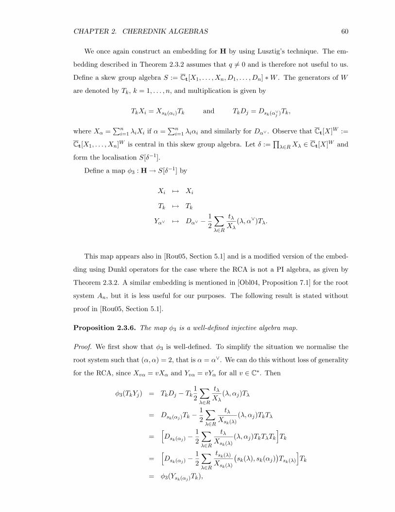
CHAPTER 2. CHEREDNIK ALGEBRAS 60
We once again construct an embedding for H by using Lusztig’s technique. The em-
bedding described in Theorem 2.3.2 assumes that q 6= 0 and is therefore not useful to us.
Define a skew group algebra S := Ct[X1, . . . , Xn, D1, . . . , Dn] ∗W . The generators of W
are denoted by Tk, k = 1, . . . , n, and multiplication is given by
TkXi = Xsk(αi)Tk and TkDj = Dsk(α∨j )Tk,
where Xα =∑n
i=1 λiXi if α =∑n
i=1 λiαi and similarly for Dα∨ . Observe that Ct[X]W :=
Ct[X1, . . . , Xn]W is central in this skew group algebra. Let δ :=∏λ∈RXλ ∈ Ct[X]W and
form the localisation S[δ−1].
Define a map φ3 : H → S[δ−1] by
Xi 7→ Xi
Tk 7→ Tk
Yα∨ 7→ Dα∨ −12
∑λ∈R
tλXλ
(λ, α∨)Tλ.
This map appears also in [Rou05, Section 5.1] and is a modified version of the embed-
ding using Dunkl operators for the case where the RCA is not a PI algebra, as given by
Theorem 2.3.2. A similar embedding is mentioned in [Obl04, Proposition 7.1] for the root
system An, but it is less useful for our purposes. The following result is stated without
proof in [Rou05, Section 5.1].
Proposition 2.3.6. The map φ3 is a well-defined injective algebra map.
Proof. We first show that φ3 is well-defined. To simplify the situation we normalise the
root system such that (α, α) = 2, that is α = α∨. We can do this without loss of generality
for the RCA, since Xvα = vXα and Yvα = vYα for all v ∈ C∗. Then
φ3(TkYj) = TkDj − Tk12
∑λ∈R
tλXλ
(λ, αj)Tλ
= Dsk(αj)Tk −12
∑λ∈R
tλXsk(λ)
(λ, αj)TkTλ
=[Dsk(αj) −
12
∑λ∈R
tλXsk(λ)
(λ, αj)TkTλTk]Tk
=[Dsk(αj) −
12
∑λ∈R
tsk(λ)
Xsk(λ)
(sk(λ), sk(αj)
)Tsk(λ)
]Tk
= φ3(Ysk(αj)Tk),
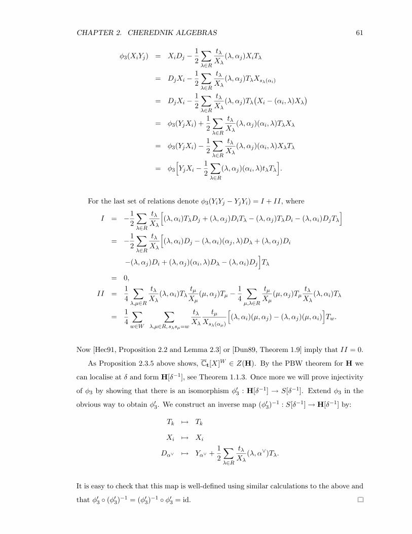
CHAPTER 2. CHEREDNIK ALGEBRAS 61
φ3(XiYj) = XiDj −12
∑λ∈R
tλXλ
(λ, αj)XiTλ
= DjXi −12
∑λ∈R
tλXλ
(λ, αj)TλXsλ(αi)
= DjXi −12
∑λ∈R
tλXλ
(λ, αj)Tλ(Xi − (αi, λ)Xλ
)= φ3(YjXi) +
12
∑λ∈R
tλXλ
(λ, αj)(αi, λ)TλXλ
= φ3(YjXi)−12
∑λ∈R
tλXλ
(λ, αj)(αi, λ)XλTλ
= φ3
[YjXi −
12
∑λ∈R
(λ, αj)(αi, λ)tλTλ].
For the last set of relations denote φ3(YiYj − YjYi) = I + II, where
I = −12
∑λ∈R
tλXλ
[(λ, αi)TλDj + (λ, αj)DiTλ − (λ, αj)TλDi − (λ, αi)DjTλ
]= −1
2
∑λ∈R
tλXλ
[(λ, αi)Dj − (λ, αi)(αj , λ)Dλ + (λ, αj)Di
−(λ, αj)Di + (λ, αj)(αi, λ)Dλ − (λ, αi)Dj
]Tλ
= 0,
II =14
∑λ,µ∈R
tλXλ
(λ, αi)TλtµXµ
(µ, αj)Tµ −14
∑µ,λ∈R
tµXµ
(µ, αj)TµtλXλ
(λ, αi)Tλ
=14
∑w∈W
∑λ,µ∈R, sλsµ=w
tλXλ
tµXsλ(αµ)
[(λ, αi)(µ, αj)− (λ, αj)(µ, αi)
]Tw.
Now [Hec91, Proposition 2.2 and Lemma 2.3] or [Dun89, Theorem 1.9] imply that II = 0.
As Proposition 2.3.5 above shows, Ct[X]W ∈ Z(H). By the PBW theorem for H we
can localise at δ and form H[δ−1], see Theorem 1.1.3. Once more we will prove injectivity
of φ3 by showing that there is an isomorphism φ′3 : H[δ−1] → S[δ−1]. Extend φ3 in the
obvious way to obtain φ′3. We construct an inverse map (φ′3)−1 : S[δ−1] → H[δ−1] by:
Tk 7→ Tk
Xi 7→ Xi
Dα∨ 7→ Yα∨ +12
∑λ∈R
tλXλ
(λ, α∨)Tλ.
It is easy to check that this map is well-defined using similar calculations to the above and
that φ′3 (φ′3)−1 = (φ′3)
−1 φ′3 = id.
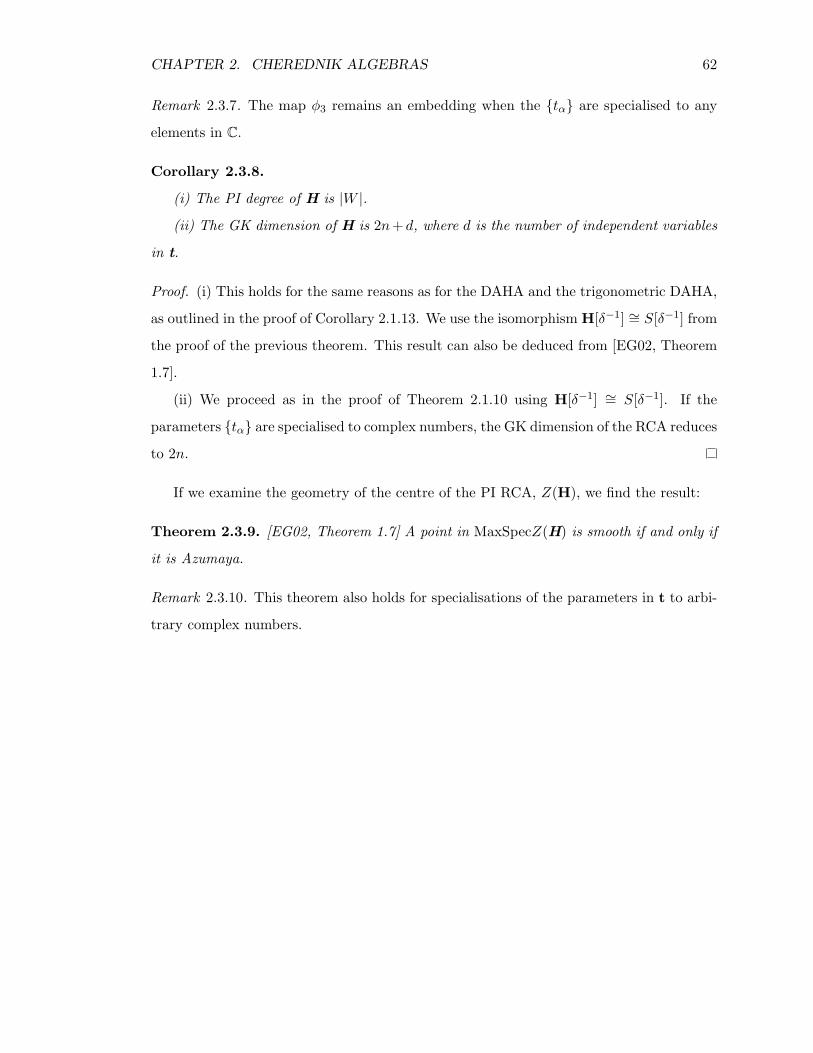
CHAPTER 2. CHEREDNIK ALGEBRAS 62
Remark 2.3.7. The map φ3 remains an embedding when the tα are specialised to any
elements in C.
Corollary 2.3.8.
(i) The PI degree of H is |W |.
(ii) The GK dimension of H is 2n+d, where d is the number of independent variables
in t.
Proof. (i) This holds for the same reasons as for the DAHA and the trigonometric DAHA,
as outlined in the proof of Corollary 2.1.13. We use the isomorphism H[δ−1] ∼= S[δ−1] from
the proof of the previous theorem. This result can also be deduced from [EG02, Theorem
1.7].
(ii) We proceed as in the proof of Theorem 2.1.10 using H[δ−1] ∼= S[δ−1]. If the
parameters tα are specialised to complex numbers, the GK dimension of the RCA reduces
to 2n.
If we examine the geometry of the centre of the PI RCA, Z(H), we find the result:
Theorem 2.3.9. [EG02, Theorem 1.7] A point in MaxSpecZ(H) is smooth if and only if
it is Azumaya.
Remark 2.3.10. This theorem also holds for specialisations of the parameters in t to arbi-
trary complex numbers.
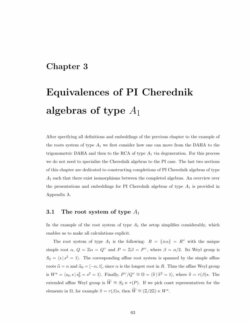
Chapter 3
Equivalences of PI Cherednik
algebras of type A1
After specifying all definitions and embeddings of the previous chapter to the example of
the roots system of type A1 we first consider how one can move from the DAHA to the
trigonometric DAHA and then to the RCA of type A1 via degeneration. For this process
we do not need to specialise the Cherednik algebras to the PI case. The last two sections
of this chapter are dedicated to constructing completions of PI Cherednik algebras of type
A1 such that there exist isomorphisms between the completed algebras. An overview over
the presentations and embeddings for PI Cherednik algebras of type A1 is provided in
Appendix A.
3.1 The root system of type A1
In the example of the root system of type A1 the setup simplifies considerably, which
enables us to make all calculations explicit.
The root system of type A1 is the following: R = ±α = R∨ with the unique
simple root α, Q = Zα = Q∨ and P = Zβ = P∨, where β = α/2. Its Weyl group is
S2 = 〈s | s2 = 1〉. The corresponding affine root system is spanned by the simple affine
roots α = α and α0 = [−α, 1], since α is the longest root in R. Thus the affine Weyl group
is W a = 〈s0, s | s20 = s2 = 1〉. Finally, P∨/Q∨ ∼= Ω = 〈π | π2 = 1〉, where π = τ(β)s. The
extended affine Weyl group is W ∼= S2 n τ(P ). If we pick coset representatives for the
elements in Ω, for example π = τ(β)s, then W ∼= (Z/2Z) nW a.
63
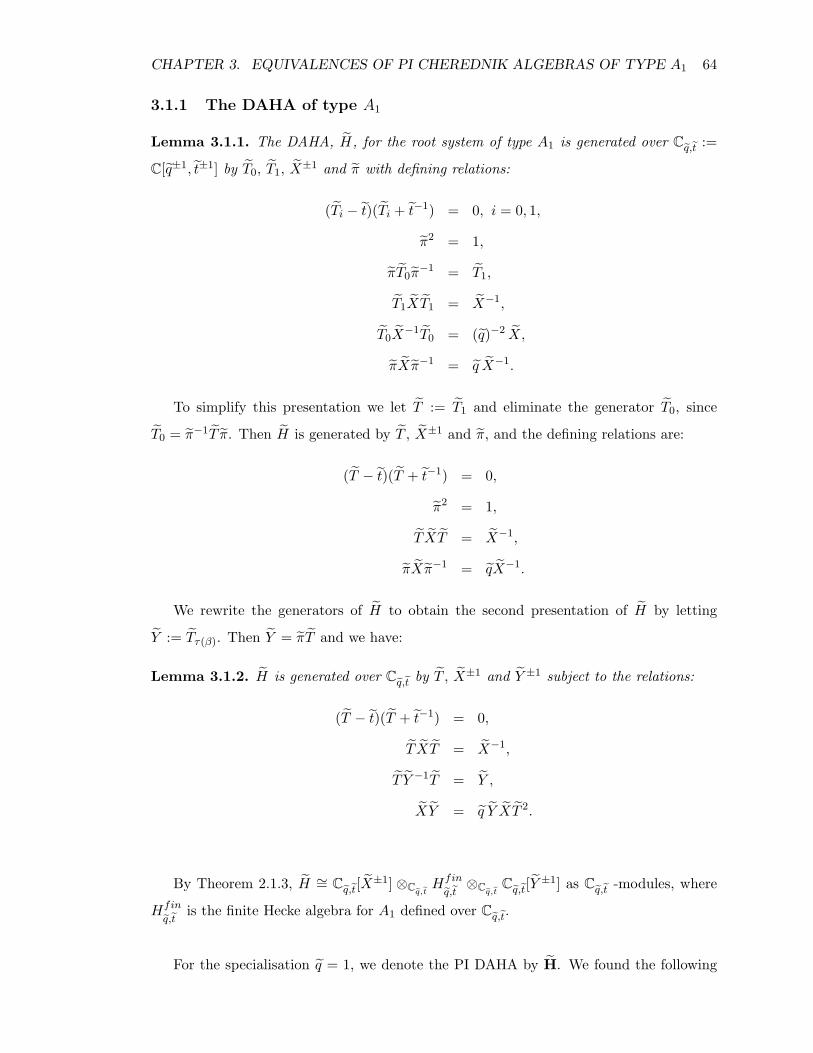
CHAPTER 3. EQUIVALENCES OF PI CHEREDNIK ALGEBRAS OF TYPE A1 64
3.1.1 The DAHA of type A1
Lemma 3.1.1. The DAHA, H, for the root system of type A1 is generated over Cq,t :=
C[q±1, t±1] by T0, T1, X±1 and π with defining relations:
(Ti − t)(Ti + t−1) = 0, i = 0, 1,
π2 = 1,
πT0π−1 = T1,
T1XT1 = X−1,
T0X−1T0 = (q)−2 X,
πXπ−1 = q X−1.
To simplify this presentation we let T := T1 and eliminate the generator T0, since
T0 = π−1T π. Then H is generated by T , X±1 and π, and the defining relations are:
(T − t)(T + t−1) = 0,
π2 = 1,
T XT = X−1,
πXπ−1 = qX−1.
We rewrite the generators of H to obtain the second presentation of H by letting
Y := Tτ(β). Then Y = πT and we have:
Lemma 3.1.2. H is generated over Cq,t by T , X±1 and Y ±1 subject to the relations:
(T − t)(T + t−1) = 0,
T XT = X−1,
T Y −1T = Y ,
XY = q Y XT 2.
By Theorem 2.1.3, H ∼= Cq,t[X±1] ⊗Cq,t
Hfin
q,t⊗Cq,t
Cq,t[Y±1] as Cq,t -modules, where
Hfin
q,tis the finite Hecke algebra for A1 defined over Cq,t.
For the specialisation q = 1, we denote the PI DAHA by H. We found the following
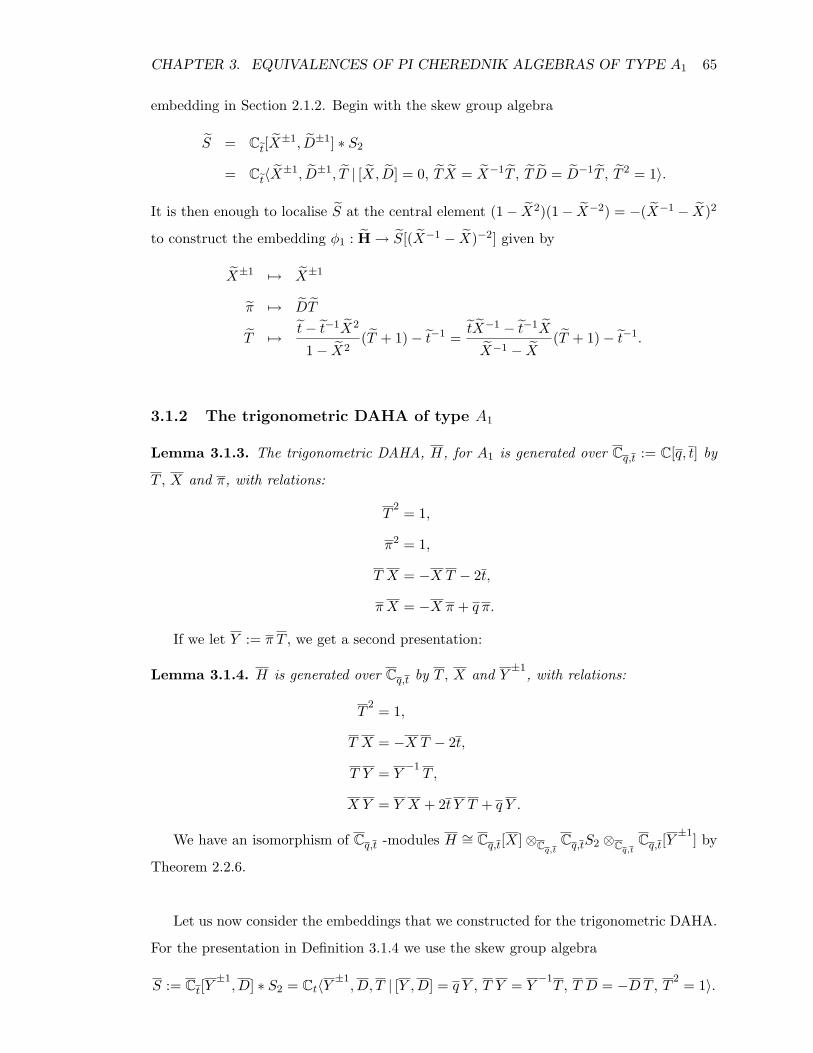
CHAPTER 3. EQUIVALENCES OF PI CHEREDNIK ALGEBRAS OF TYPE A1 65
embedding in Section 2.1.2. Begin with the skew group algebra
S = Ct[X±1, D±1] ∗ S2
= Ct〈X±1, D±1, T | [X, D] = 0, T X = X−1T , T D = D−1T , T 2 = 1〉.
It is then enough to localise S at the central element (1− X2)(1− X−2) = −(X−1 − X)2
to construct the embedding φ1 : H → S[(X−1 − X)−2] given by
X±1 7→ X±1
π 7→ DT
T 7→ t− t−1X2
1− X2(T + 1)− t−1 =
tX−1 − t−1X
X−1 − X(T + 1)− t−1.
3.1.2 The trigonometric DAHA of type A1
Lemma 3.1.3. The trigonometric DAHA, H, for A1 is generated over Cq,t := C[q, t] by
T , X and π, with relations:
T2 = 1,
π2 = 1,
T X = −X T − 2t,
π X = −X π + q π.
If we let Y := π T , we get a second presentation:
Lemma 3.1.4. H is generated over Cq,t by T , X and Y ±1, with relations:
T2 = 1,
T X = −X T − 2t,
T Y = Y−1T ,
X Y = Y X + 2t Y T + q Y .
We have an isomorphism of Cq,t -modules H ∼= Cq,t[X]⊗Cq,tCq,tS2 ⊗Cq,t
Cq,t[Y±1] by
Theorem 2.2.6.
Let us now consider the embeddings that we constructed for the trigonometric DAHA.
For the presentation in Definition 3.1.4 we use the skew group algebra
S := Ct[Y±1, D] ∗ S2 = Ct〈Y
±1, D, T | [Y ,D] = q Y , T Y = Y
−1T , T D = −DT, T
2 = 1〉.
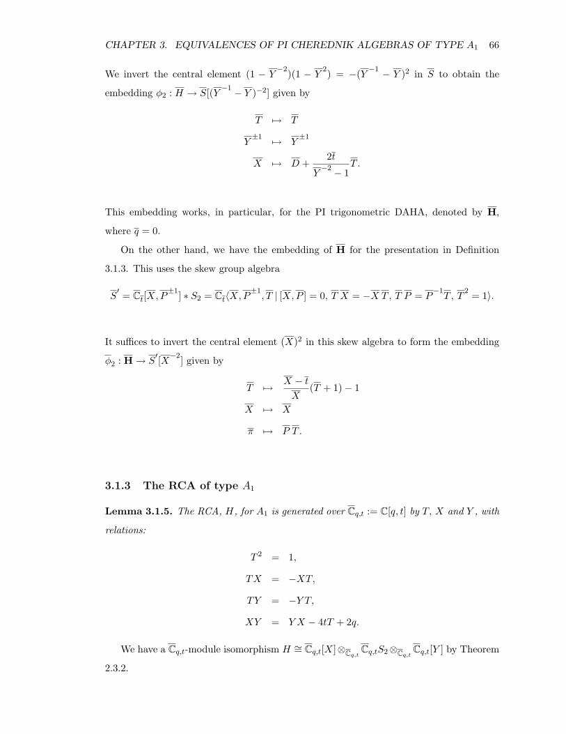
CHAPTER 3. EQUIVALENCES OF PI CHEREDNIK ALGEBRAS OF TYPE A1 66
We invert the central element (1 − Y−2)(1 − Y
2) = −(Y −1 − Y )2 in S to obtain the
embedding φ2 : H → S[(Y −1 − Y )−2] given by
T 7→ T
Y±1 7→ Y
±1
X 7→ D +2t
Y−2 − 1
T .
This embedding works, in particular, for the PI trigonometric DAHA, denoted by H,
where q = 0.
On the other hand, we have the embedding of H for the presentation in Definition
3.1.3. This uses the skew group algebra
S′ = Ct[X,P
±1] ∗ S2 = Ct〈X,P±1, T | [X,P ] = 0, T X = −X T, T P = P
−1T , T
2 = 1〉.
It suffices to invert the central element (X)2 in this skew algebra to form the embedding
φ2 : H → S′[X−2] given by
T 7→ X − t
X(T + 1)− 1
X 7→ X
π 7→ P T .
3.1.3 The RCA of type A1
Lemma 3.1.5. The RCA, H, for A1 is generated over Cq,t := C[q, t] by T, X and Y , with
relations:
T 2 = 1,
TX = −XT,
TY = −Y T,
XY = Y X − 4tT + 2q.
We have a Cq,t-module isomorphism H ∼= Cq,t[X]⊗Cq,tCq,tS2⊗Cq,t
Cq,t[Y ] by Theorem
2.3.2.
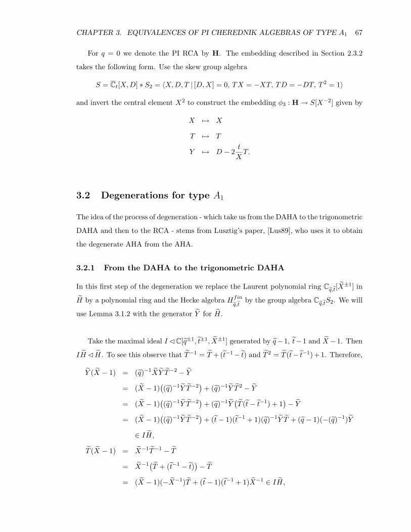
CHAPTER 3. EQUIVALENCES OF PI CHEREDNIK ALGEBRAS OF TYPE A1 67
For q = 0 we denote the PI RCA by H. The embedding described in Section 2.3.2
takes the following form. Use the skew group algebra
S = Ct[X,D] ∗ S2 = 〈X,D, T | [D,X] = 0, TX = −XT, TD = −DT, T 2 = 1〉
and invert the central element X2 to construct the embedding φ3 : H → S[X−2] given by
X 7→ X
T 7→ T
Y 7→ D − 2t
XT.
3.2 Degenerations for type A1
The idea of the process of degeneration - which take us from the DAHA to the trigonometric
DAHA and then to the RCA - stems from Lusztig’s paper, [Lus89], who uses it to obtain
the degenerate AHA from the AHA.
3.2.1 From the DAHA to the trigonometric DAHA
In this first step of the degeneration we replace the Laurent polynomial ring Cq,t[X±1] in
H by a polynomial ring and the Hecke algebra Hfin
q,tby the group algebra Cq,tS2. We will
use Lemma 3.1.2 with the generator Y for H.
Take the maximal ideal ICC[q±1, t±1, X±1] generated by q−1, t−1 and X−1. Then
IHC H. To see this observe that T−1 = T +(t−1− t) and T 2 = T (t− t−1)+1. Therefore,
Y (X − 1) = (q)−1XY T−2 − Y
= (X − 1)((q)−1Y T−2
)+ (q)−1Y T 2 − Y
= (X − 1)((q)−1Y T−2
)+ (q)−1Y
(T (t− t−1) + 1
)− Y
= (X − 1)((q)−1Y T−2
)+ (t− 1)(t−1 + 1)(q)−1Y T + (q − 1)(−(q)−1)Y
∈ IH,
T (X − 1) = X−1T−1 − T
= X−1(T + (t−1 − t)
)− T
= (X − 1)(−X−1)T + (t− 1)(t−1 + 1)X−1 ∈ IH,
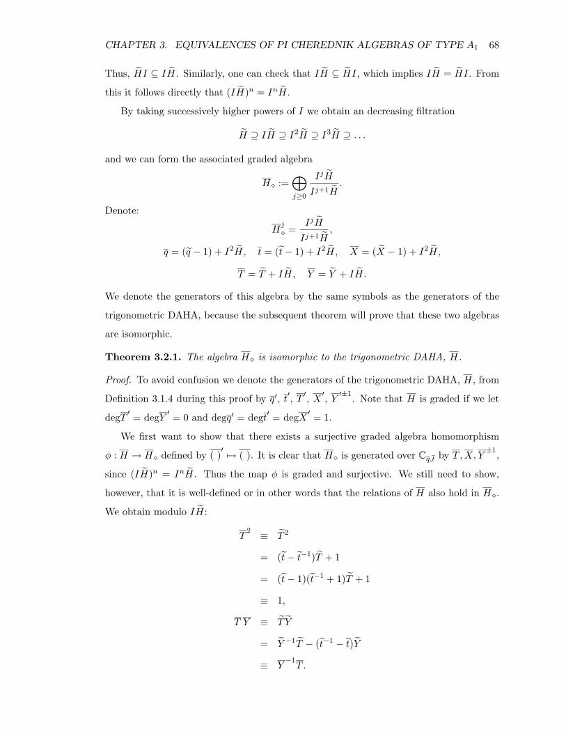
CHAPTER 3. EQUIVALENCES OF PI CHEREDNIK ALGEBRAS OF TYPE A1 68
Thus, HI ⊆ IH. Similarly, one can check that IH ⊆ HI, which implies IH = HI. From
this it follows directly that (IH)n = InH.
By taking successively higher powers of I we obtain an decreasing filtration
H ⊇ IH ⊇ I2H ⊇ I3H ⊇ . . .
and we can form the associated graded algebra
H :=⊕j≥0
IjH
Ij+1H.
Denote:
Hj =
IjH
Ij+1H,
q = (q − 1) + I2H, t = (t− 1) + I2H, X = (X − 1) + I2H,
T = T + IH, Y = Y + IH.
We denote the generators of this algebra by the same symbols as the generators of the
trigonometric DAHA, because the subsequent theorem will prove that these two algebras
are isomorphic.
Theorem 3.2.1. The algebra H is isomorphic to the trigonometric DAHA, H.
Proof. To avoid confusion we denote the generators of the trigonometric DAHA, H, from
Definition 3.1.4 during this proof by q′, t′, T ′, X ′, Y ′±1. Note that H is graded if we let
degT ′ = degY ′ = 0 and degq′ = degt′ = degX ′ = 1.
We first want to show that there exists a surjective graded algebra homomorphism
φ : H → H defined by ( )′ 7→ ( ). It is clear that H is generated over Cq,t by T ,X, Y ±1,
since (IH)n = InH. Thus the map φ is graded and surjective. We still need to show,
however, that it is well-defined or in other words that the relations of H also hold in H.
We obtain modulo IH:
T2 ≡ T 2
= (t− t−1)T + 1
= (t− 1)(t−1 + 1)T + 1
≡ 1,
T Y ≡ T Y
= Y −1T − (t−1 − t)Y
≡ Y−1T .
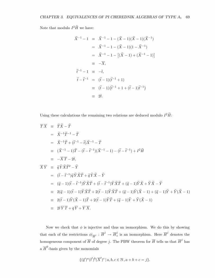
CHAPTER 3. EQUIVALENCES OF PI CHEREDNIK ALGEBRAS OF TYPE A1 69
Note that modulo I2H we have:
X−1 − 1 ≡ X−1 − 1− (X − 1)(X − 1)(X−1)
= X−1 − 1− (X − 1)(1− X−1)
= X−1 − 1−[(X − 1) + (X−1 − 1)
]≡ −X,
t−1 − 1 ≡ −t,
t− t−1 = (t− 1)(t−1 + 1)
≡ (t− 1)(t−1 + 1 + (t− 1)t−1
)≡ 2t.
Using these calculations the remaining two relations are deduced modulo I2H:
T X ≡ T X − T
= X−1T−1 − T
= X−1T + (t−1 − t)X−1 − T
≡ (X−1 − 1)T − (t− t−1)(X−1 − 1)− (t− t−1) + I2H
≡ −X T − 2t,
X Y ≡ q Y XT 2 − Y
= (t− t−1)q Y XT + q Y X − Y
= (q − 1)(t− t−1)Y XT + (t− t−1)Y XT + (q − 1)Y X + Y X − Y
≡ 2(q − 1)(t− 1)Y XT + 2(t− 1)Y XT + (q − 1)Y (X − 1) + (q − 1)Y + Y (X − 1)
≡ 2(t− 1)Y (X − 1)T + 2(t− 1)Y T + (q − 1)Y + Y (X − 1)
≡ 2t Y T + q Y + Y X.
Now we check that φ is injective and thus an isomorphism. We do this by showing
that each of the restrictions φ|H
j : Hj → Hj is an isomorphism. Here Hj denotes the
homogeneous component of H of degree j. The PBW theorem for H tells us that Hj has
a H0-basis given by the monomials
(q′)a(t′)b(X ′)c | a, b, c ∈ N , a+ b+ c = j.
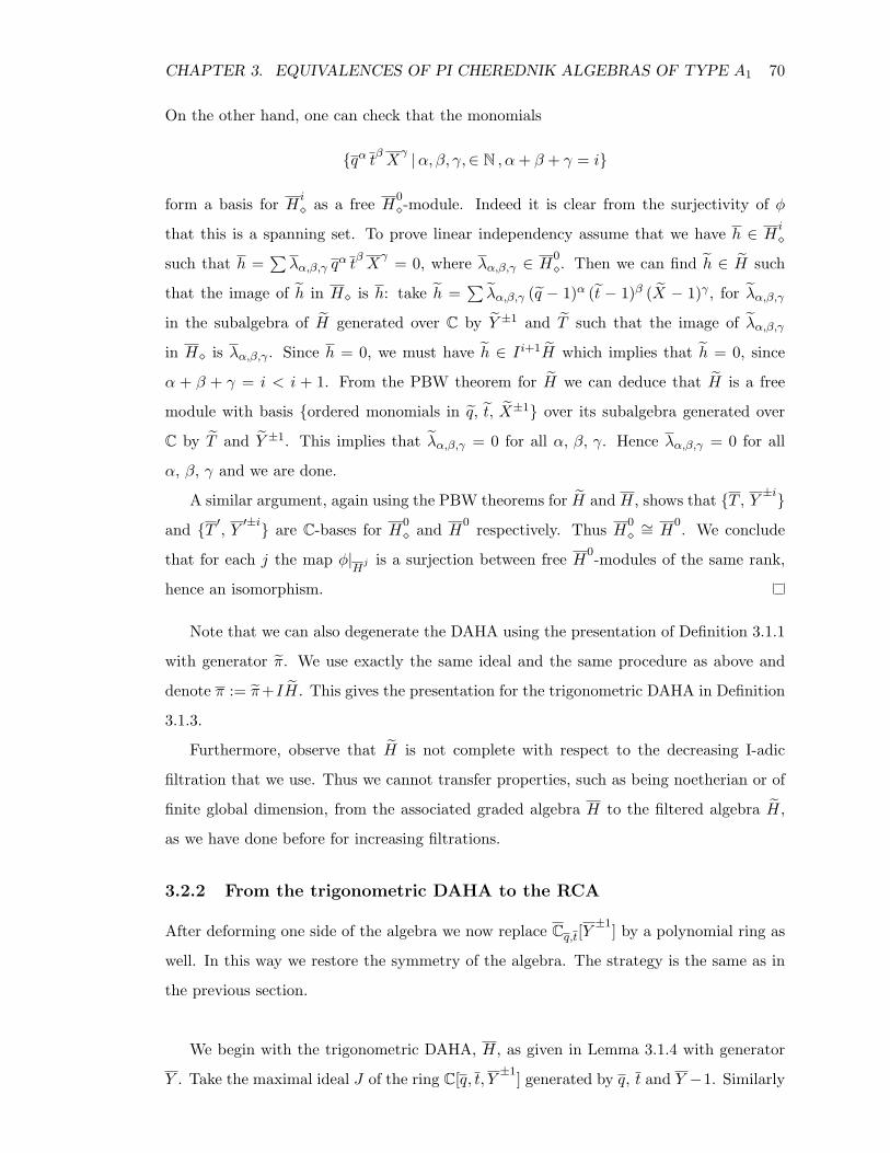
CHAPTER 3. EQUIVALENCES OF PI CHEREDNIK ALGEBRAS OF TYPE A1 70
On the other hand, one can check that the monomials
qα tβ Xγ |α, β, γ,∈ N , α+ β + γ = i
form a basis for H i as a free H0
-module. Indeed it is clear from the surjectivity of φ
that this is a spanning set. To prove linear independency assume that we have h ∈ Hi
such that h =∑λα,β,γ q
α tβXγ = 0, where λα,β,γ ∈ H
0. Then we can find h ∈ H such
that the image of h in H is h: take h =∑λα,β,γ (q − 1)α (t − 1)β (X − 1)γ , for λα,β,γ
in the subalgebra of H generated over C by Y ±1 and T such that the image of λα,β,γ
in H is λα,β,γ . Since h = 0, we must have h ∈ Ii+1H which implies that h = 0, since
α + β + γ = i < i + 1. From the PBW theorem for H we can deduce that H is a free
module with basis ordered monomials in q, t, X±1 over its subalgebra generated over
C by T and Y ±1. This implies that λα,β,γ = 0 for all α, β, γ. Hence λα,β,γ = 0 for all
α, β, γ and we are done.
A similar argument, again using the PBW theorems for H and H, shows that T , Y ±i
and T ′, Y ′±i are C-bases for H0 and H
0 respectively. Thus H0∼= H
0. We conclude
that for each j the map φ|H
j is a surjection between free H0-modules of the same rank,
hence an isomorphism.
Note that we can also degenerate the DAHA using the presentation of Definition 3.1.1
with generator π. We use exactly the same ideal and the same procedure as above and
denote π := π+IH. This gives the presentation for the trigonometric DAHA in Definition
3.1.3.
Furthermore, observe that H is not complete with respect to the decreasing I-adic
filtration that we use. Thus we cannot transfer properties, such as being noetherian or of
finite global dimension, from the associated graded algebra H to the filtered algebra H,
as we have done before for increasing filtrations.
3.2.2 From the trigonometric DAHA to the RCA
After deforming one side of the algebra we now replace Cq,t[Y±1] by a polynomial ring as
well. In this way we restore the symmetry of the algebra. The strategy is the same as in
the previous section.
We begin with the trigonometric DAHA, H, as given in Lemma 3.1.4 with generator
Y . Take the maximal ideal J of the ring C[q, t, Y ±1] generated by q, t and Y −1. Similarly
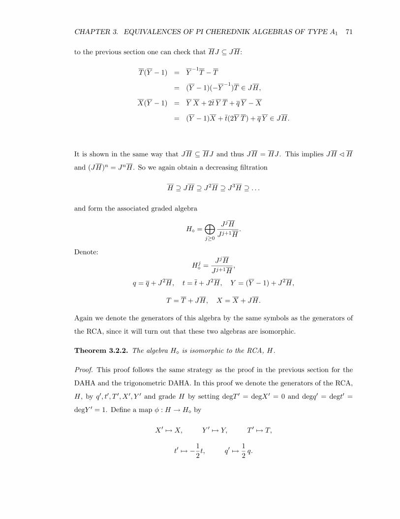
CHAPTER 3. EQUIVALENCES OF PI CHEREDNIK ALGEBRAS OF TYPE A1 71
to the previous section one can check that HJ ⊆ JH:
T (Y − 1) = Y−1T − T
= (Y − 1)(−Y −1)T ∈ JH,
X(Y − 1) = Y X + 2t Y T + q Y −X
= (Y − 1)X + t(2Y T ) + q Y ∈ JH.
It is shown in the same way that JH ⊆ HJ and thus JH = HJ . This implies JH CH
and (JH)n = JnH. So we again obtain a decreasing filtration
H ⊇ JH ⊇ J2H ⊇ J3H ⊇ . . .
and form the associated graded algebra
H =⊕j≥0
J jH
J j+1H.
Denote:
Hj =
J jH
J j+1H,
q = q + J2H, t = t+ J2H, Y = (Y − 1) + J2H,
T = T + JH, X = X + JH.
Again we denote the generators of this algebra by the same symbols as the generators of
the RCA, since it will turn out that these two algebras are isomorphic.
Theorem 3.2.2. The algebra H is isomorphic to the RCA, H.
Proof. This proof follows the same strategy as the proof in the previous section for the
DAHA and the trigonometric DAHA. In this proof we denote the generators of the RCA,
H, by q′, t′, T ′, X ′, Y ′ and grade H by setting degT ′ = degX ′ = 0 and degq′ = degt′ =
degY ′ = 1. Define a map φ : H → H by
X ′ 7→ X, Y ′ 7→ Y, T ′ 7→ T,
t′ 7→ −12t, q′ 7→ 1
2q.
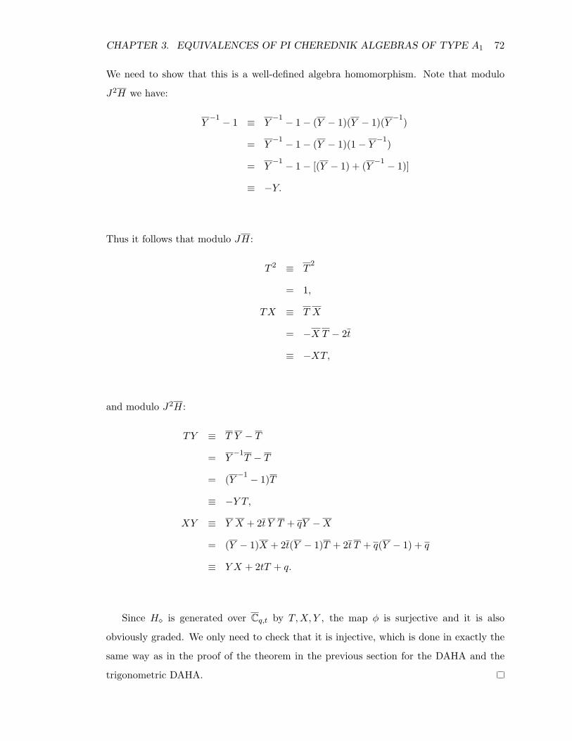
CHAPTER 3. EQUIVALENCES OF PI CHEREDNIK ALGEBRAS OF TYPE A1 72
We need to show that this is a well-defined algebra homomorphism. Note that modulo
J2H we have:
Y−1 − 1 ≡ Y
−1 − 1− (Y − 1)(Y − 1)(Y −1)
= Y−1 − 1− (Y − 1)(1− Y
−1)
= Y−1 − 1− [(Y − 1) + (Y −1 − 1)]
≡ −Y.
Thus it follows that modulo JH:
T 2 ≡ T2
= 1,
TX ≡ T X
= −X T − 2t
≡ −XT,
and modulo J2H:
TY ≡ T Y − T
= Y−1T − T
= (Y −1 − 1)T
≡ −Y T,
XY ≡ Y X + 2t Y T + qY −X
= (Y − 1)X + 2t(Y − 1)T + 2t T + q(Y − 1) + q
≡ Y X + 2tT + q.
Since H is generated over Cq,t by T,X, Y , the map φ is surjective and it is also
obviously graded. We only need to check that it is injective, which is done in exactly the
same way as in the proof of the theorem in the previous section for the DAHA and the
trigonometric DAHA.
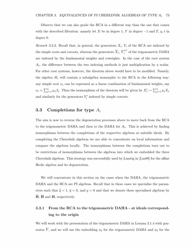
CHAPTER 3. EQUIVALENCES OF PI CHEREDNIK ALGEBRAS OF TYPE A1 73
Observe that we can also grade the RCA in a different way than the one that comes
with the described filtration: namely let X be in degree 1, Y in degree −1 and T, q, t in
degree 0.
Remark 3.2.3. Recall that, in general, the generators Xi, Yi of the RCA are indexed by
the simple roots and coroots, whereas the generators Xi, Y±1i of the trigonometric DAHA
are indexed by the fundamental weights and coweights. In the case of the root system
A1, the difference between the two indexing methods is just multiplication by a scalar.
For other root systems, however, the theorem above would have to be modified. Namely,
the algebra H will contain a subalgebra isomorphic to the RCA in the following way:
any simple root αi can be expressed as a linear combination of fundamental weights, say
αi =∑n
j=1 µjβj . Then the isomorphism of the theorem will be given by X ′i 7→∑n
j=1 µjXj
and similarly for the generators Y ′i indexed by simple coroots.
3.3 Completions for type A1
The aim is now to reverse the degeneration processes above to move back from the RCA
to the trigonometric DAHA and then to the DAHA for A1. This is achieved by finding
isomorphisms between the completions of the respective algebras at suitable ideals. By
completing the Cherednik algebras we are able to concentrate on local information and
compare the algebras locally. The isomorphisms between the completions turn out to
be restrictions of isomorphisms between the algebras into which we embedded the three
Cherednik algebras. This strategy was successfully used by Lusztig in [Lus89] for the affine
Hecke algebra and its degeneration.
We will concentrate in this section on the cases when the DAHA, the trigonometric
DAHA and the RCA are PI algebras. Recall that in these cases we specialise the param-
eters such that q = 1, q = 0, and q = 0 and that we denote these specialised algebras by
H, H and H, respectively.
3.3.1 From the RCA to the trigonometric DAHA - at ideals correspond-
ing to the origin
We will work with the presentation of the trigonometric DAHA in Lemma 3.1.4 with gen-
erator Y , and we will use the embedding φ2 for the trigonometric DAHA and φ3 for the
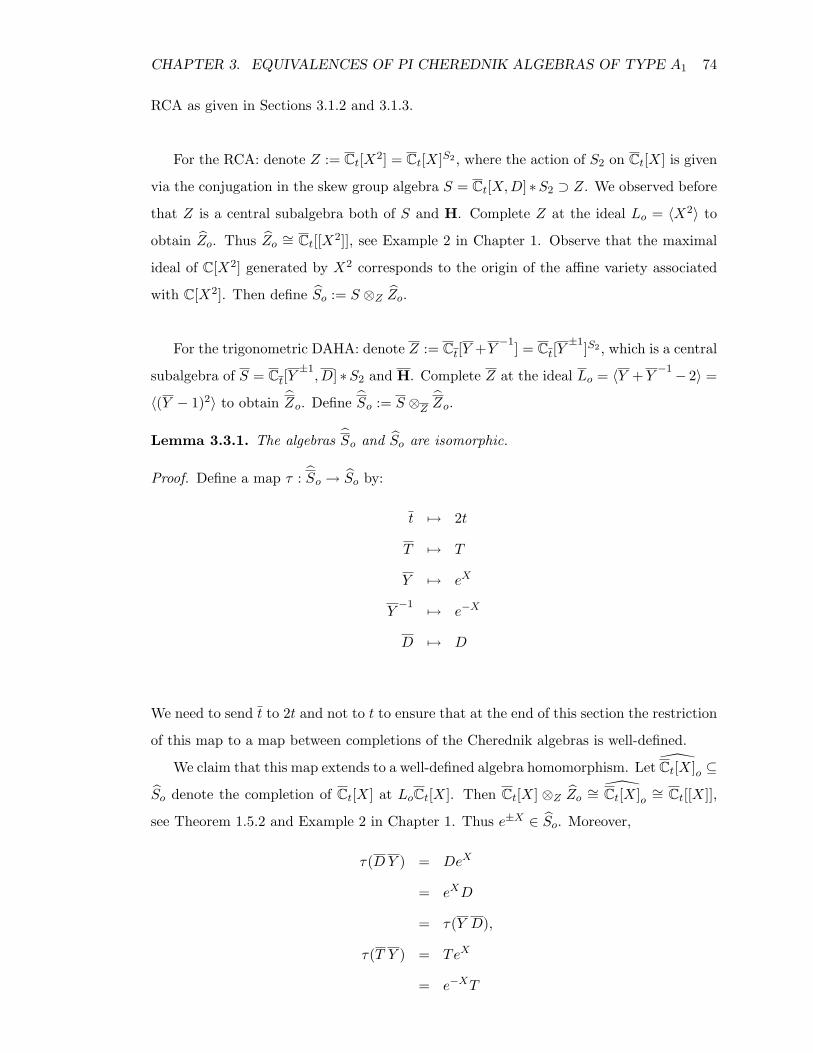
CHAPTER 3. EQUIVALENCES OF PI CHEREDNIK ALGEBRAS OF TYPE A1 74
RCA as given in Sections 3.1.2 and 3.1.3.
For the RCA: denote Z := Ct[X2] = Ct[X]S2 , where the action of S2 on Ct[X] is given
via the conjugation in the skew group algebra S = Ct[X,D] ∗S2 ⊃ Z. We observed before
that Z is a central subalgebra both of S and H. Complete Z at the ideal Lo = 〈X2〉 to
obtain Zo. Thus Zo ∼= Ct[[X2]], see Example 2 in Chapter 1. Observe that the maximal
ideal of C[X2] generated by X2 corresponds to the origin of the affine variety associated
with C[X2]. Then define So := S ⊗Z Zo.
For the trigonometric DAHA: denote Z := Ct[Y +Y −1] = Ct[Y±1]S2 , which is a central
subalgebra of S = Ct[Y±1, D] ∗S2 and H. Complete Z at the ideal Lo = 〈Y +Y
−1− 2〉 =
〈(Y − 1)2〉 to obtain Zo. Define So := S ⊗Z Zo.
Lemma 3.3.1. The algebras So and So are isomorphic.
Proof. Define a map τ : So → So by:
t 7→ 2t
T 7→ T
Y 7→ eX
Y−1 7→ e−X
D 7→ D
We need to send t to 2t and not to t to ensure that at the end of this section the restriction
of this map to a map between completions of the Cherednik algebras is well-defined.
We claim that this map extends to a well-defined algebra homomorphism. Let Ct[X]o ⊆
So denote the completion of Ct[X] at LoCt[X]. Then Ct[X] ⊗Z Zo ∼= Ct[X]o ∼= Ct[[X]],
see Theorem 1.5.2 and Example 2 in Chapter 1. Thus e±X ∈ So. Moreover,
τ(DY ) = DeX
= eXD
= τ(Y D),
τ(T Y ) = TeX
= e−XT
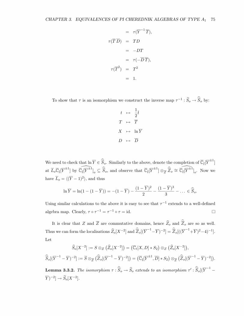
CHAPTER 3. EQUIVALENCES OF PI CHEREDNIK ALGEBRAS OF TYPE A1 75
= τ(Y −1T ),
τ(T D) = TD
= −DT
= τ(−DT ),
τ(T 2) = T 2
= 1.
To show that τ is an isomorphism we construct the inverse map τ−1 : So → So by:
t 7→ 12t
T 7→ T
X 7→ lnY
D 7→ D
We need to check that lnY ∈ So. Similarly to the above, denote the completion of Ct[Y±1]
at LoCt[Y±1] by Ct[Y
±1]o ⊆ So, and observe that Ct[Y±1] ⊗Z Zo ∼= Ct[Y
±1]o. Now we
have Lo = 〈(Y − 1)2〉, and thus
lnY = ln(1− (1− Y )) = −(1− Y )− (1− Y )2
2− (1− Y )3
3− . . . ∈ So.
Using similar calculations to the above it is easy to see that τ−1 extends to a well-defined
algebra map. Clearly, τ τ−1 = τ−1 τ = id.
It is clear that Z and Z are commutative domains, hence Zo and Zo are so as well.
Thus we can form the localisations Zo[X−2] and Zo[(Y−1−Y )−2] = Zo[((Y
−1+Y )2−4)−1].
Let
So[X−2] := S ⊗Z(Zo[X−2]
)=
(Ct[X,D] ∗ S2
)⊗Z
(Zo[X−2]
),
So[(Y−1 − Y )−2] := S ⊗Z
(Zo[(Y
−1 − Y )−2])
=(Ct[Y
±1, D] ∗ S2
)⊗Z
(Zo[(Y
−1 − Y )−2]).
Lemma 3.3.2. The isomorphism τ : So → So extends to an isomorphism τ ′ : So[(Y−1 −
Y )−2] → So[X−2].
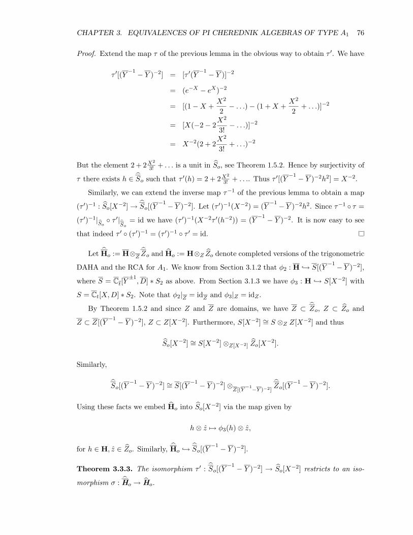
CHAPTER 3. EQUIVALENCES OF PI CHEREDNIK ALGEBRAS OF TYPE A1 76
Proof. Extend the map τ of the previous lemma in the obvious way to obtain τ ′. We have
τ ′[(Y −1 − Y )−2] = [τ ′(Y −1 − Y )]−2
= (e−X − eX)−2
= [(1−X +X2
2− . . .)− (1 +X +
X2
2+ . . .)]−2
= [X(−2− 2X2
3!− . . .)]−2
= X−2(2 + 2X2
3!+ . . .)−2
But the element 2 + 2X2
3! + . . . is a unit in So, see Theorem 1.5.2. Hence by surjectivity of
τ there exists h ∈ So such that τ ′(h) = 2 + 2X2
3! + . . .. Thus τ ′[(Y −1 − Y )−2h2] = X−2.
Similarly, we can extend the inverse map τ−1 of the previous lemma to obtain a map
(τ ′)−1 : So[X−2] → So[(Y−1 − Y )−2]. Let (τ ′)−1(X−2) = (Y −1 − Y )−2h2. Since τ−1 τ =
(τ ′)−1|So τ ′|
So= id we have (τ ′)−1(X−2τ ′(h−2)) = (Y −1 − Y )−2. It is now easy to see
that indeed τ ′ (τ ′)−1 = (τ ′)−1 τ ′ = id.
Let Ho := H⊗Z Zo and Ho := H⊗Z Zo denote completed versions of the trigonometric
DAHA and the RCA for A1. We know from Section 3.1.2 that φ2 : H → S[(Y −1− Y )−2],
where S = Ct[Y±1, D] ∗ S2 as above. From Section 3.1.3 we have φ3 : H → S[X−2] with
S = Ct[X,D] ∗ S2. Note that φ2|Z = idZ and φ3|Z = idZ .
By Theorem 1.5.2 and since Z and Z are domains, we have Z ⊂ Zo, Z ⊂ Zo and
Z ⊂ Z[(Y −1 − Y )−2], Z ⊂ Z[X−2]. Furthermore, S[X−2] ∼= S ⊗Z Z[X−2] and thus
So[X−2] ∼= S[X−2]⊗Z[X−2] Zo[X−2].
Similarly,
So[(Y−1 − Y )−2] ∼= S[(Y −1 − Y )−2]⊗
Z[(Y−1−Y )−2]
Zo[(Y−1 − Y )−2].
Using these facts we embed Ho into So[X−2] via the map given by
h⊗ z 7→ φ3(h)⊗ z,
for h ∈ H, z ∈ Zo. Similarly, Ho → So[(Y−1 − Y )−2].
Theorem 3.3.3. The isomorphism τ ′ : So[(Y−1 − Y )−2] → So[X−2] restricts to an iso-
morphism σ : Ho → Ho.
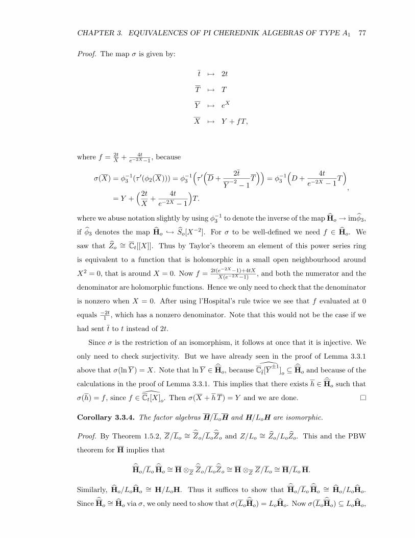
CHAPTER 3. EQUIVALENCES OF PI CHEREDNIK ALGEBRAS OF TYPE A1 77
Proof. The map σ is given by:
t 7→ 2t
T 7→ T
Y 7→ eX
X 7→ Y + fT,
where f = 2tX + 4t
e−2X−1, because
σ(X) = φ−13 (τ ′(φ2(X))) = φ−1
3
(τ ′
(D +
2t
Y−2 − 1
T))
= φ−13
(D +
4te−2X − 1
T)
= Y +(2tX
+4t
e−2X − 1
)T.
,
where we abuse notation slightly by using φ−13 to denote the inverse of the map Ho → imφ3,
if φ3 denotes the map Ho → So[X−2]. For σ to be well-defined we need f ∈ Ho. We
saw that Zo ∼= Ct[[X]]. Thus by Taylor’s theorem an element of this power series ring
is equivalent to a function that is holomorphic in a small open neighbourhood around
X2 = 0, that is around X = 0. Now f = 2t(e−2X−1)+4tXX(e−2X−1)
, and both the numerator and the
denominator are holomorphic functions. Hence we only need to check that the denominator
is nonzero when X = 0. After using l’Hospital’s rule twice we see that f evaluated at 0
equals −2t1 , which has a nonzero denominator. Note that this would not be the case if we
had sent t to t instead of 2t.
Since σ is the restriction of an isomorphism, it follows at once that it is injective. We
only need to check surjectivity. But we have already seen in the proof of Lemma 3.3.1
above that σ(lnY ) = X. Note that lnY ∈ Ho, because Ct[Y±1]o ⊆ Ho and because of the
calculations in the proof of Lemma 3.3.1. This implies that there exists h ∈ Ho such that
σ(h) = f , since f ∈ Ct[X]o. Then σ(X + hT ) = Y and we are done.
Corollary 3.3.4. The factor algebras H/LoH and H/LoH are isomorphic.
Proof. By Theorem 1.5.2, Z/Lo ∼= Zo/LoZo and Z/Lo ∼= Zo/LoZo. This and the PBW
theorem for H implies that
Ho/Lo Ho∼= H⊗Z Zo/LoZo ∼= H⊗Z Z/Lo ∼= H/LoH.
Similarly, Ho/LoHo∼= H/LoH. Thus it suffices to show that Ho/Lo Ho
∼= Ho/LoHo.
Since Ho∼= Ho via σ, we only need to show that σ(LoHo) = LoHo. Now σ(LoHo) ⊆ LoHo,
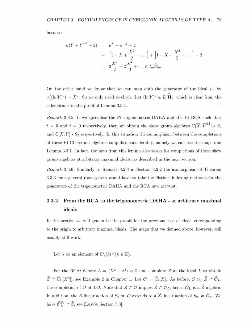
CHAPTER 3. EQUIVALENCES OF PI CHEREDNIK ALGEBRAS OF TYPE A1 78
because
σ(Y + Y−1 − 2) = eX + e−X − 2
=[1 +X +
X2
2+ . . .
]+
[1−X +
X2
2− . . .
]− 2
= 2X2
2+ 2
X4
4!+ . . . ∈ LoHo.
On the other hand we know that we can map onto the generator of the ideal Lo by
σ((lnY )2) = X2. So we only need to check that (lnY )2 ∈ LoHo, which is clear from the
calculations in the proof of Lemma 3.3.1.
Remark 3.3.5. If we specialise the PI trigonometric DAHA and the PI RCA such that
t = 0 and t = 0 respectively, then we obtain the skew group algebras C[X,Y ±1] ∗ S2
and C[X,Y ] ∗ S2 respectively. In this situation the isomorphism between the completions
of these PI Cherednik algebras simplifies considerably, namely we can use the map from
Lemma 3.3.1. In fact, the map from this lemma also works for completions of these skew
group algebras at arbitrary maximal ideals, as described in the next section.
Remark 3.3.6. Similarly to Remark 3.2.3 in Section 3.2.2 the isomorphism of Theorem
3.3.3 for a general root system would have to take the distinct indexing methods for the
generators of the trigonometric DAHA and the RCA into account.
3.3.2 From the RCA to the trigonometric DAHA - at arbitrary maximal
ideals
In this section we will generalise the proofs for the previous case of ideals corresponding
to the origin to arbitrary maximal ideals. The maps that we defined above, however, will
usually still work.
Let λ be an element of C\kiπ | k ∈ Z.
For the RCA: denote L = 〈X2 − λ2〉 C Z and complete Z at the ideal L to obtain
Z ∼= Ct[[X2]], see Example 2 in Chapter 1. Let O := Ct[X]. As before, O ⊗Z Z ∼= OL,
the completion of O at LO. Note that Z ⊂ O implies Z ⊂ OL, hence OL is a Z-algebra.
In addition, the Z-linear action of S2 on O extends to a Z-linear action of S2 on OL. We
have OS2L∼= Z, see [Lus89, Section 7.3].
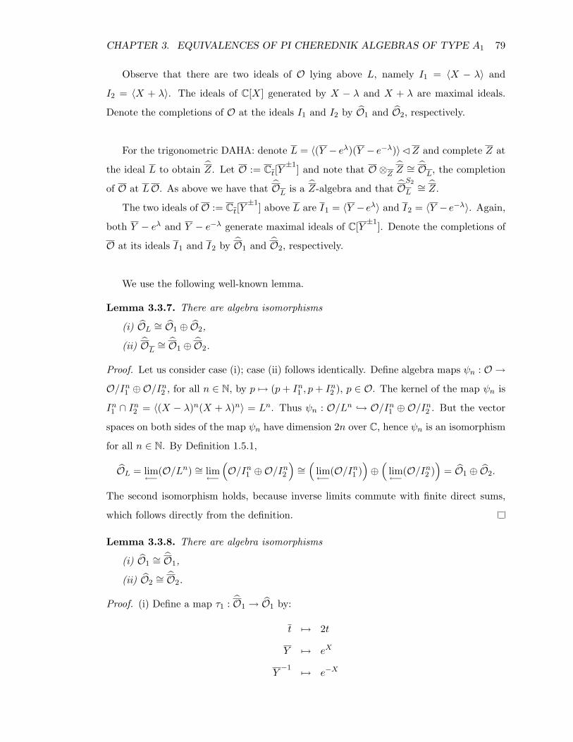
CHAPTER 3. EQUIVALENCES OF PI CHEREDNIK ALGEBRAS OF TYPE A1 79
Observe that there are two ideals of O lying above L, namely I1 = 〈X − λ〉 and
I2 = 〈X + λ〉. The ideals of C[X] generated by X − λ and X + λ are maximal ideals.
Denote the completions of O at the ideals I1 and I2 by O1 and O2, respectively.
For the trigonometric DAHA: denote L = 〈(Y − eλ)(Y − e−λ)〉CZ and complete Z at
the ideal L to obtain Z. Let O := Ct[Y±1] and note that O ⊗Z Z ∼= OL, the completion
of O at LO. As above we have that OL is a Z-algebra and that OS2
L∼= Z.
The two ideals of O := Ct[Y±1] above L are I1 = 〈Y − eλ〉 and I2 = 〈Y − e−λ〉. Again,
both Y − eλ and Y − e−λ generate maximal ideals of C[Y ±1]. Denote the completions of
O at its ideals I1 and I2 by O1 and O2, respectively.
We use the following well-known lemma.
Lemma 3.3.7. There are algebra isomorphisms
(i) OL ∼= O1 ⊕ O2,
(ii) OL∼= O1 ⊕ O2.
Proof. Let us consider case (i); case (ii) follows identically. Define algebra maps ψn : O →
O/In1 ⊕O/In2 , for all n ∈ N, by p 7→ (p+ In1 , p+ In2 ), p ∈ O. The kernel of the map ψn is
In1 ∩ In2 = 〈(X − λ)n(X + λ)n〉 = Ln. Thus ψn : O/Ln → O/In1 ⊕ O/In2 . But the vector
spaces on both sides of the map ψn have dimension 2n over C, hence ψn is an isomorphism
for all n ∈ N. By Definition 1.5.1,
OL = lim←−
(O/Ln) ∼= lim←−
(O/In1 ⊕O/In2
)∼=
(lim←−
(O/In1 ))⊕
(lim←−
(O/In2 ))
= O1 ⊕ O2.
The second isomorphism holds, because inverse limits commute with finite direct sums,
which follows directly from the definition.
Lemma 3.3.8. There are algebra isomorphisms
(i) O1∼= O1,
(ii) O2∼= O2.
Proof. (i) Define a map τ1 : O1 → O1 by:
t 7→ 2t
Y 7→ eX
Y−1 7→ e−X
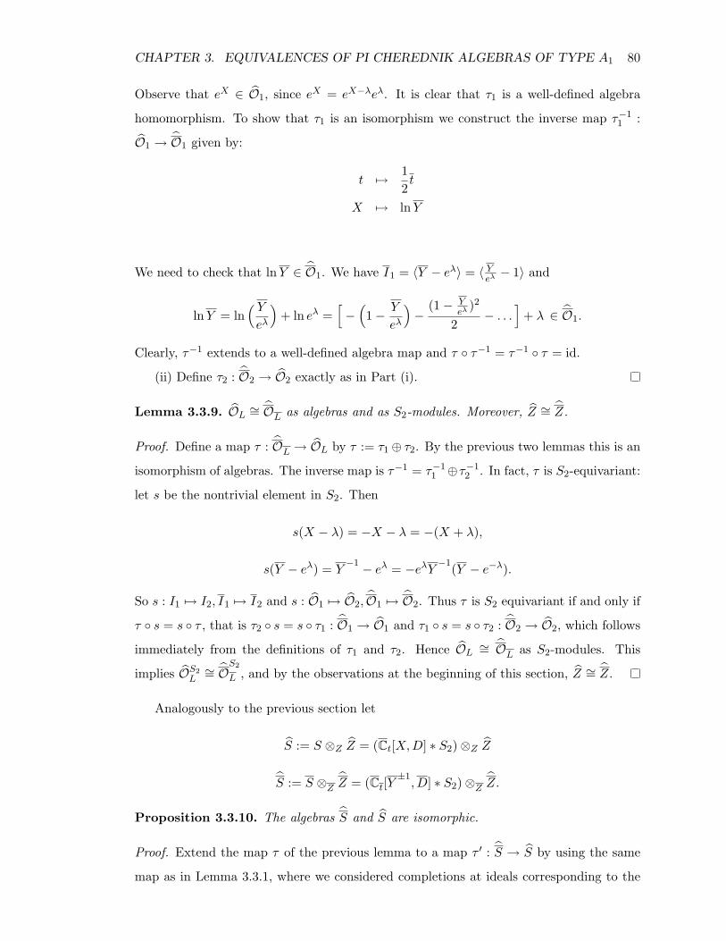
CHAPTER 3. EQUIVALENCES OF PI CHEREDNIK ALGEBRAS OF TYPE A1 80
Observe that eX ∈ O1, since eX = eX−λeλ. It is clear that τ1 is a well-defined algebra
homomorphism. To show that τ1 is an isomorphism we construct the inverse map τ−11 :
O1 → O1 given by:
t 7→ 12t
X 7→ lnY
We need to check that lnY ∈ O1. We have I1 = 〈Y − eλ〉 = 〈 Yeλ − 1〉 and
lnY = ln( Yeλ
)+ ln eλ =
[−
(1− Y
eλ
)−
(1− Yeλ )2
2− . . .
]+ λ ∈ O1.
Clearly, τ−1 extends to a well-defined algebra map and τ τ−1 = τ−1 τ = id.
(ii) Define τ2 : O2 → O2 exactly as in Part (i).
Lemma 3.3.9. OL ∼= OL as algebras and as S2-modules. Moreover, Z ∼= Z.
Proof. Define a map τ : OL → OL by τ := τ1⊕ τ2. By the previous two lemmas this is an
isomorphism of algebras. The inverse map is τ−1 = τ−11 ⊕τ−1
2 . In fact, τ is S2-equivariant:
let s be the nontrivial element in S2. Then
s(X − λ) = −X − λ = −(X + λ),
s(Y − eλ) = Y−1 − eλ = −eλY −1(Y − e−λ).
So s : I1 7→ I2, I1 7→ I2 and s : O1 7→ O2, O1 7→ O2. Thus τ is S2 equivariant if and only if
τ s = s τ , that is τ2 s = s τ1 : O1 → O1 and τ1 s = s τ2 : O2 → O2, which follows
immediately from the definitions of τ1 and τ2. Hence OL ∼= OL as S2-modules. This
implies OS2L∼= O
S2
L , and by the observations at the beginning of this section, Z ∼= Z.
Analogously to the previous section let
S := S ⊗Z Z = (Ct[X,D] ∗ S2)⊗Z Z
S := S ⊗Z Z = (Ct[Y±1, D] ∗ S2)⊗Z Z.
Proposition 3.3.10. The algebras S and S are isomorphic.
Proof. Extend the map τ of the previous lemma to a map τ ′ : S → S by using the same
map as in Lemma 3.3.1, where we considered completions at ideals corresponding to the
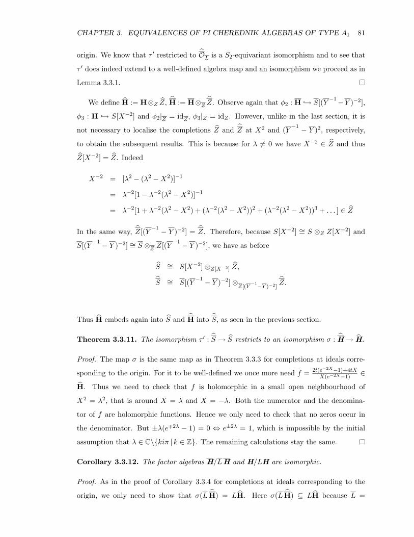
CHAPTER 3. EQUIVALENCES OF PI CHEREDNIK ALGEBRAS OF TYPE A1 81
origin. We know that τ ′ restricted to OL is a S2-equivariant isomorphism and to see that
τ ′ does indeed extend to a well-defined algebra map and an isomorphism we proceed as in
Lemma 3.3.1.
We define H := H⊗Z Z, H := H⊗Z Z. Observe again that φ2 : H → S[(Y −1−Y )−2],
φ3 : H → S[X−2] and φ2|Z = idZ , φ3|Z = idZ . However, unlike in the last section, it is
not necessary to localise the completions Z and Z at X2 and (Y −1 − Y )2, respectively,
to obtain the subsequent results. This is because for λ 6= 0 we have X−2 ∈ Z and thus
Z[X−2] = Z. Indeed
X−2 = [λ2 − (λ2 −X2)]−1
= λ−2[1− λ−2(λ2 −X2)]−1
= λ−2[1 + λ−2(λ2 −X2) + (λ−2(λ2 −X2))2 + (λ−2(λ2 −X2))3 + . . . ] ∈ Z
In the same way, Z[(Y −1 − Y )−2] = Z. Therefore, because S[X−2] ∼= S ⊗Z Z[X−2] and
S[(Y −1 − Y )−2] ∼= S ⊗Z Z[(Y −1 − Y )−2], we have as before
S ∼= S[X−2]⊗Z[X−2] Z,
S ∼= S[(Y −1 − Y )−2]⊗Z[(Y
−1−Y )−2]Z.
Thus H embeds again into S and H into S, as seen in the previous section.
Theorem 3.3.11. The isomorphism τ ′ : S → S restricts to an isomorphism σ : H→ H.
Proof. The map σ is the same map as in Theorem 3.3.3 for completions at ideals corre-
sponding to the origin. For it to be well-defined we once more need f = 2t(e−2X−1)+4tXX(e−2X−1)
∈
H. Thus we need to check that f is holomorphic in a small open neighbourhood of
X2 = λ2, that is around X = λ and X = −λ. Both the numerator and the denomina-
tor of f are holomorphic functions. Hence we only need to check that no zeros occur in
the denominator. But ±λ(e∓2λ − 1) = 0 ⇔ e±2λ = 1, which is impossible by the initial
assumption that λ ∈ C\kiπ | k ∈ Z. The remaining calculations stay the same.
Corollary 3.3.12. The factor algebras H/LH and H/LH are isomorphic.
Proof. As in the proof of Corollary 3.3.4 for completions at ideals corresponding to the
origin, we only need to show that σ(L H) = LH. Here σ(L H) ⊆ LH because L =
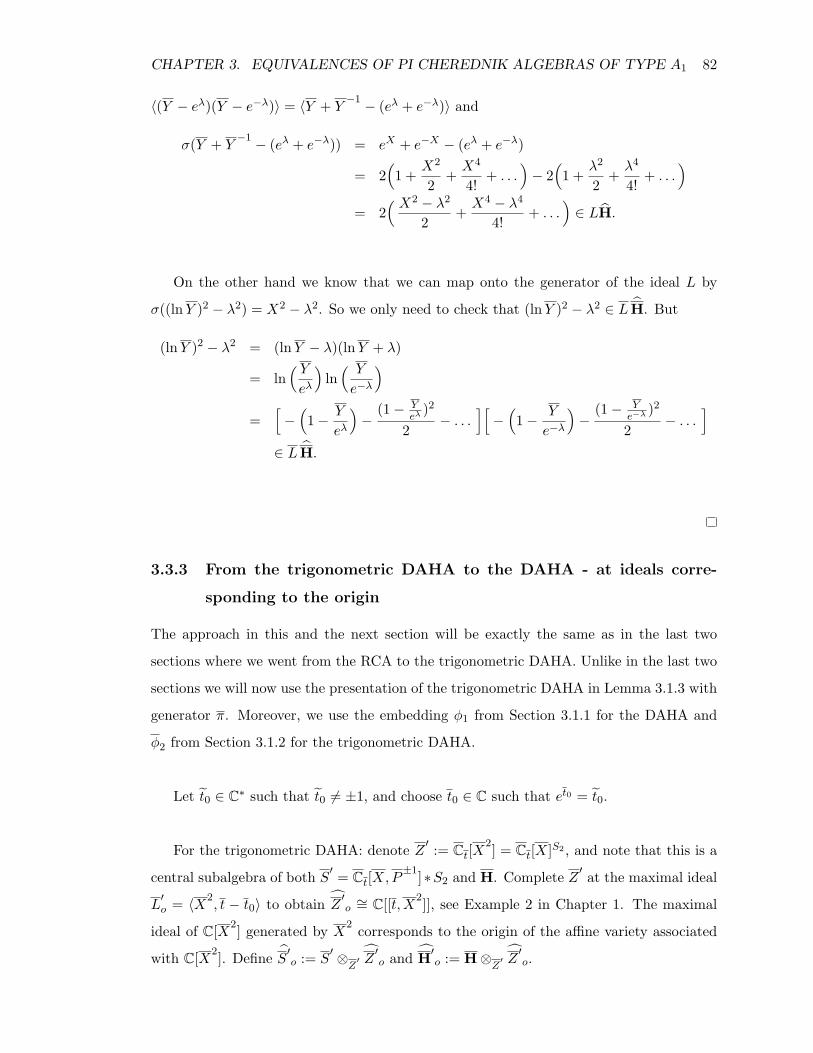
CHAPTER 3. EQUIVALENCES OF PI CHEREDNIK ALGEBRAS OF TYPE A1 82
〈(Y − eλ)(Y − e−λ)〉 = 〈Y + Y−1 − (eλ + e−λ)〉 and
σ(Y + Y−1 − (eλ + e−λ)) = eX + e−X − (eλ + e−λ)
= 2(1 +
X2
2+X4
4!+ . . .
)− 2
(1 +
λ2
2+λ4
4!+ . . .
)= 2
( X2 − λ2
2+X4 − λ4
4!+ . . .
)∈ LH.
On the other hand we know that we can map onto the generator of the ideal L by
σ((lnY )2 − λ2) = X2 − λ2. So we only need to check that (lnY )2 − λ2 ∈ L H. But
(lnY )2 − λ2 = (lnY − λ)(lnY + λ)
= ln( Yeλ
)ln
( Y
e−λ
)=
[−
(1− Y
eλ
)−
(1− Yeλ )2
2− . . .
][−
(1− Y
e−λ
)−
(1− Ye−λ )2
2− . . .
]∈ L H.
3.3.3 From the trigonometric DAHA to the DAHA - at ideals corre-
sponding to the origin
The approach in this and the next section will be exactly the same as in the last two
sections where we went from the RCA to the trigonometric DAHA. Unlike in the last two
sections we will now use the presentation of the trigonometric DAHA in Lemma 3.1.3 with
generator π. Moreover, we use the embedding φ1 from Section 3.1.1 for the DAHA and
φ2 from Section 3.1.2 for the trigonometric DAHA.
Let t0 ∈ C∗ such that t0 6= ±1, and choose t0 ∈ C such that et0 = t0.
For the trigonometric DAHA: denote Z ′ := Ct[X2] = Ct[X]S2 , and note that this is a
central subalgebra of both S′ = Ct[X,P±1]∗S2 and H. Complete Z ′ at the maximal ideal
L′o = 〈X2
, t − t0〉 to obtain Z′o∼= C[[t,X2]], see Example 2 in Chapter 1. The maximal
ideal of C[X2] generated by X2 corresponds to the origin of the affine variety associated
with C[X2]. Define S′o := S′ ⊗
Z′ Z′o and H′o := H⊗
Z′ Z′o.
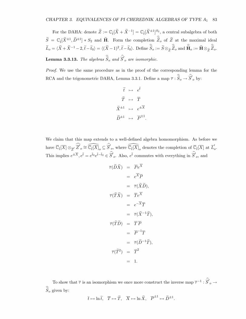
CHAPTER 3. EQUIVALENCES OF PI CHEREDNIK ALGEBRAS OF TYPE A1 83
For the DAHA: denote Z := Ct[X + X−1] = Ct[X±1]S2 , a central subalgebra of both
S = Ct[X±1, D±1] ∗ S2 and H. Form the completion
Zo of Z at the maximal ideal
Lo = 〈X+ X−1−2, t− t0〉 = 〈(X−1)2, t− t0〉. Define So := S⊗
ZZo and Ho := H⊗
ZZo.
Lemma 3.3.13. The algebras So and S′o are isomorphic.
Proof. We use the same procedure as in the proof of the corresponding lemma for the
RCA and the trigonometric DAHA, Lemma 3.3.1. Define a map τ : So → S
′o by:
t 7→ et
T 7→ T
X±1 7→ e±X
D±1 7→ P±1.
We claim that this map extends to a well-defined algebra homomorphism. As before we
have Ct[X]⊗Z′ Z′o∼= Ct[X]o ⊆ S
′o, where Ct[X]o denotes the completion of Ct[X] at L′o.
This implies e±X , et = et0et−t0 ∈ S′o. Also, et commutes with everything in S′o, and
τ(DX) = PeX
= eXP
= τ(XD),
τ(T X) = TeX
= e−XT
= τ(X−1T ),
τ(T D) = T P
= P−1T
= τ(D−1T ),
τ(T 2) = T2
= 1.
To show that τ is an isomorphism we once more construct the inverse map τ−1 : S′o →So given by:
t 7→ ln t, T 7→ T , X 7→ ln X, P±1 7→ D±1.
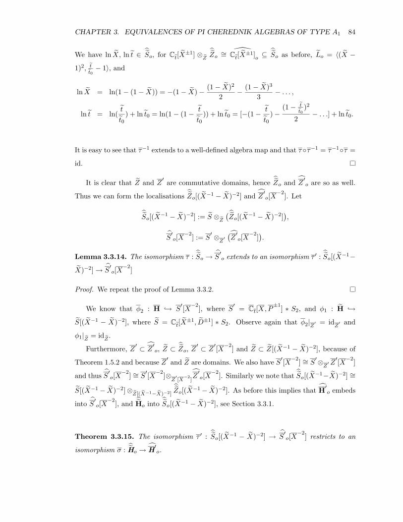
CHAPTER 3. EQUIVALENCES OF PI CHEREDNIK ALGEBRAS OF TYPE A1 84
We have ln X, ln t ∈ So, for Ct[X
±1] ⊗Z
Zo ∼= Ct[X±1]o ⊆
So as before, Lo = 〈(X −
1)2, tt0− 1〉, and
ln X = ln(1− (1− X)) = −(1− X)− (1− X)2
2− (1− X)3
3− . . . ,
ln t = ln(t
t0) + ln t0 = ln(1− (1− t
t0)) + ln t0 = [−(1− t
t0)−
(1− tt0
)2
2− . . .] + ln t0.
It is easy to see that τ−1 extends to a well-defined algebra map and that τ τ−1 = τ−1τ =
id.
It is clear that Z and Z′ are commutative domains, hence
Zo and Z′o are so as well.
Thus we can form the localisations Zo[(X−1 − X)−2] and Z ′o[X
−2]. Let
So[(X−1 − X)−2] := S ⊗
Z
(Zo[(X−1 − X)−2]
),
S′o[X
−2] := S′ ⊗
Z′(Z′o[X
−2]).
Lemma 3.3.14. The isomorphism τ : So → S
′o extends to an isomorphism τ ′ :
So[(X−1−
X)−2] → S′o[X
−2]
Proof. We repeat the proof of Lemma 3.3.2.
We know that φ2 : H → S′[X−2], where S
′ = Ct[X,P±1] ∗ S2, and φ1 : H →
S[(X−1 − X)−2], where S = Ct[X±1, D±1] ∗ S2. Observe again that φ2|Z′ = id
Z′ and
φ1|Z = idZ.
Furthermore, Z ′ ⊂ Z′o, Z ⊂
Zo, Z′ ⊂ Z
′[X−2] and Z ⊂ Z[(X−1 − X)−2], because of
Theorem 1.5.2 and because Z ′ and Z are domains. We also have S′[X−2] ∼= S′⊗
Z′Z′[X−2]
and thus S′o[X−2] ∼= S
′[X−2]⊗Z′[X
−2]Z′o[X
−2]. Similarly we note that So[(X−1−X)−2] ∼=
S[(X−1 − X)−2]⊗Z[(X−1−X)−2]
Zo[(X−1 − X)−2]. As before this implies that H′o embeds
into S′o[X−2], and Ho into
So[(X−1 − X)−2], see Section 3.3.1.
Theorem 3.3.15. The isomorphism τ ′ : So[(X−1 − X)−2] → S
′o[X
−2] restricts to an
isomorphism σ : Ho → H
′o.
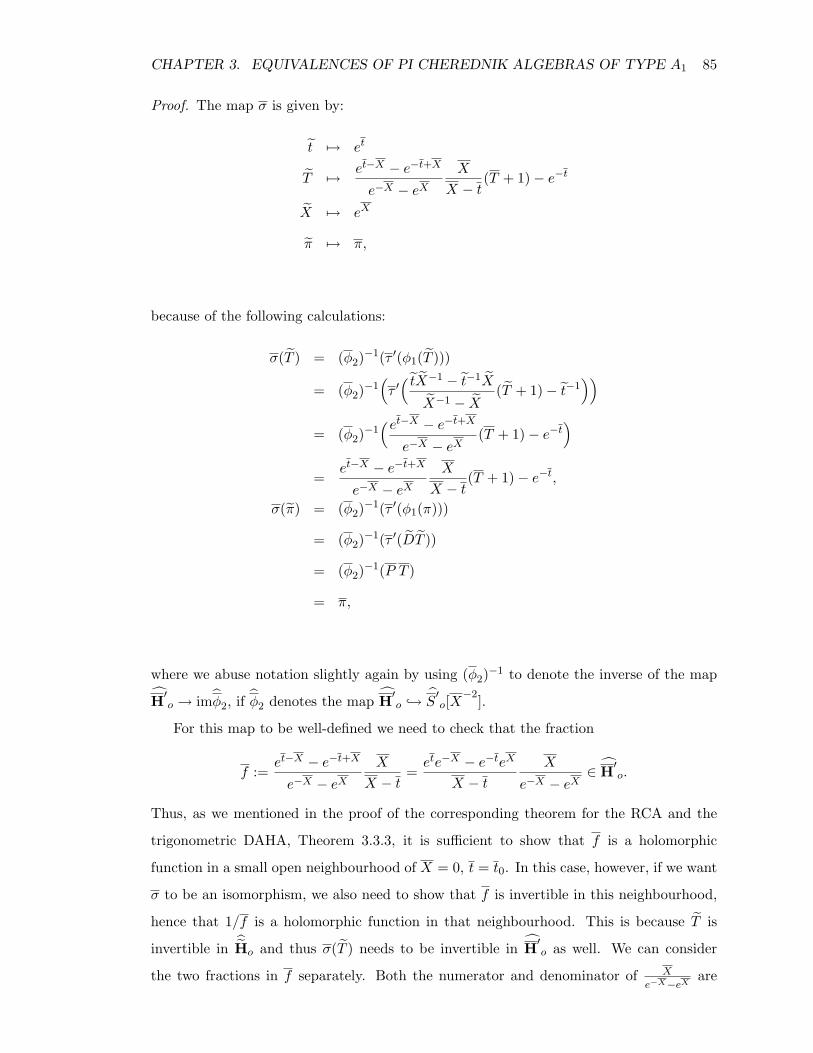
CHAPTER 3. EQUIVALENCES OF PI CHEREDNIK ALGEBRAS OF TYPE A1 85
Proof. The map σ is given by:
t 7→ et
T 7→ et−X − e−t+X
e−X − eXX
X − t(T + 1)− e−t
X 7→ eX
π 7→ π,
because of the following calculations:
σ(T ) = (φ2)−1(τ ′(φ1(T )))
= (φ2)−1
(τ ′
( tX−1 − t−1X
X−1 − X(T + 1)− t−1
))= (φ2)
−1(et−X − e−t+X
e−X − eX(T + 1)− e−t
)=
et−X − e−t+X
e−X − eXX
X − t(T + 1)− e−t,
σ(π) = (φ2)−1(τ ′(φ1(π)))
= (φ2)−1(τ ′(DT ))
= (φ2)−1(P T )
= π,
where we abuse notation slightly again by using (φ2)−1 to denote the inverse of the map
H′o → imφ2, if φ2 denotes the map H′o → S′o[X
−2].
For this map to be well-defined we need to check that the fraction
f :=et−X − e−t+X
e−X − eXX
X − t=ete−X − e−teX
X − t
X
e−X − eX∈ H′o.
Thus, as we mentioned in the proof of the corresponding theorem for the RCA and the
trigonometric DAHA, Theorem 3.3.3, it is sufficient to show that f is a holomorphic
function in a small open neighbourhood of X = 0, t = t0. In this case, however, if we want
σ to be an isomorphism, we also need to show that f is invertible in this neighbourhood,
hence that 1/f is a holomorphic function in that neighbourhood. This is because T is
invertible in Ho and thus σ(T ) needs to be invertible in H′o as well. We can consider
the two fractions in f separately. Both the numerator and denominator of X
e−X−eXare
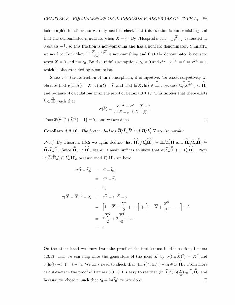
CHAPTER 3. EQUIVALENCES OF PI CHEREDNIK ALGEBRAS OF TYPE A1 86
holomorphic functions, so we only need to check that this fraction is non-vanishing and
that the denominator is nonzero when X = 0. By l’Hospital’s rule, X
e−X−eXevaluated at
0 equals −12 , so this fraction is non-vanishing and has a nonzero denominator. Similarly,
we need to check that ete−X−e−teX
X−t is non-vanishing and that the denominator is nonzero
when X = 0 and t = t0. By the initial assumptions, t0 6= 0 and et0 − e−t0 = 0 ⇔ e2t0 = 1,
which is also excluded by assumption.
Since σ is the restriction of an isomorphism, it is injective. To check surjectivity we
observe that σ(ln X) = X, σ(ln t) = t, and that ln X, ln t ∈ Ho, because Ct[X±1]o ⊆Ho
and because of calculations from the proof of Lemma 3.3.13. This implies that there exists
h ∈ Ho such that
σ(h) =e−X − eX
et−X − e−t+XX − t
X.
Thus σ(h(T + t−1)− 1
)= T , and we are done.
Corollary 3.3.16. The factor algebras H/LoH and H/L′oH are isomorphic.
Proof. By Theorem 1.5.2 we again deduce that H′o/L′oH′o∼= H/L′oH and Ho/Lo
Ho∼=
H/LoH. Since Ho∼= H′o via σ, it again suffices to show that σ(Lo
Ho) = L′o H′o. Now
σ(LoHo) ⊆ L
′o H′o because mod L′o H
′o we have
σ(t− t0) = et − t0
≡ et0 − t0
= 0,
σ(X + X−1 − 2) = eX + e−X − 2
=[1 +X +
X2
2+ . . .
]+
[1−X +
X2
2− . . .
]− 2
= 2X
2
2+ 2
X4
4!+ . . .
≡ 0.
On the other hand we know from the proof of the first lemma in this section, Lemma
3.3.13, that we can map onto the generators of the ideal L′ by σ((ln X)2) = X2 and
σ(ln(t)− t0) = t− t0. We only need to check that (ln X)2, ln(t)− t0 ∈ LoHo. From more
calculations in the proof of Lemma 3.3.13 it is easy to see that (ln X)2, ln( tt0
) ∈ LoHo and
because we chose t0 such that t0 = ln(t0) we are done.
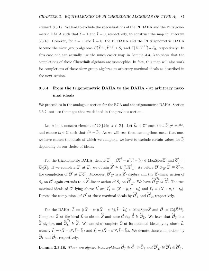
CHAPTER 3. EQUIVALENCES OF PI CHEREDNIK ALGEBRAS OF TYPE A1 87
Remark 3.3.17. We had to exclude the specialisations of the PI DAHA and the PI trigono-
metric DAHA such that t = 1 and t = 0, respectively, to construct the map in Theorem
3.3.15. However, for t = 1 and t = 0, the PI DAHA and the PI trigonometric DAHA
become the skew group algebras C[X±1, Y ±1] ∗ S2 and C[X,Y ±1] ∗ S2, respectively. In
this case one can actually use the much easier map in Lemma 3.3.13 to show that the
completions of these Cherednik algebras are isomorphic. In fact, this map will also work
for completions of these skew group algebras at arbitrary maximal ideals as described in
the next section.
3.3.4 From the trigonometric DAHA to the DAHA - at arbitrary max-
imal ideals
We proceed as in the analogous section for the RCA and the trigonometric DAHA, Section
3.3.2, but use the maps that we defined in the previous section.
Let µ be a nonzero element of C\kiπ | k ∈ Z. Let t0 ∈ C∗ such that t0 6= ±e±µ,
and choose t0 ∈ C such that et0 = t0. As we will see, these assumptions mean that once
we have chosen the ideals at which we complete, we have to exclude certain values for t0
depending on our choice of ideals.
For the trigonometric DAHA: denote L′ = 〈X2 − µ2, t − t0〉 ∈ MaxSpecZ ′ and O′ :=
Ct[X]. If we complete Z ′ at L′, we obtain Z′ ∼= C[[t,X2]]. As before O′ ⊗
Z′ Z′ ∼= O′
L′ ,
the completion of O′ at L′O′. Moreover, O′L′ is a Z ′-algebra and the Z ′-linear action of
S2 on O′ again extends to a Z ′-linear action of S2 on O′L′ . We have O′
S2
L′ ∼= Z
′. The two
maximal ideals of O′ lying above L′ are I ′1 = 〈X − µ, t − t0〉 and I′2 = 〈X + µ, t − t0〉.
Denote the completions of O′ at these maximal ideals by O′1 and O′2, respectively.
For the DAHA: L := 〈(X − eµ)(X − e−µ), t − t0〉 ∈ MaxSpecZ and O := Ct[X±1].
Complete Z at the ideal L to obtain Z and note O ⊗
ZZ ∼= O
L. We have that O
Lis a
Z-algebra and OS2
L∼= Z. We can also complete O at its maximal ideals lying above L,
namely I1 = 〈X − eµ, t− t0〉 and I2 = 〈X − e−µ, t− t0〉. We denote these completions byO1 and O2, respectively.
Lemma 3.3.18. There are algebra isomorphisms OL∼= O1 ⊕
O2 and O′L′ ∼= O′1 ⊕ O
′2.
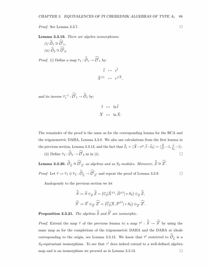
CHAPTER 3. EQUIVALENCES OF PI CHEREDNIK ALGEBRAS OF TYPE A1 88
Proof. See Lemma 3.3.7.
Lemma 3.3.19. There are algebra isomorphisms
(i) O1∼= O′1,
(ii) O2∼= O′2.
Proof. (i) Define a map τ1 : O1 → O′1 by:
t 7→ et
X±1 7→ e±X ,
and its inverse τ−11 : O′1 →
O1 by:
t 7→ ln t
X 7→ ln X.
The remainder of the proof is the same as for the corresponding lemma for the RCA and
the trigonometric DAHA, Lemma 3.3.8. We also use calculations from the first lemma in
the previous section, Lemma 3.3.13, and the fact that I1 = 〈X−eµ, t− t0〉 = 〈 Xeµ−1, tt0−1〉.
(ii) Define τ2 : O2 → O′2 as in (i).
Lemma 3.3.20. OL∼= O′
L′ as algebras and as S2-modules. Moreover,
Z ∼= Z′.
Proof. Let τ := τ1 ⊕ τ2 : OL→ O′
L′ and repeat the proof of Lemma 3.3.9.
Analogously to the previous section we let
S := S ⊗
ZZ =
(Ct[X
±1, D±1] ∗ S2
)⊗Z
Z,
S′ := S
′ ⊗Z′ Z′ =
(Ct[X,P
±1] ∗ S2
)⊗Z′ Z′.
Proposition 3.3.21. The algebras S and S′ are isomorphic.
Proof. Extend the map τ of the previous lemma to a map τ ′ : S → S
′ by using the
same map as for the completions of the trigonometric DAHA and the DAHA at ideals
corresponding to the origin, see Lemma 3.3.13. We know that τ ′ restricted to OL
is a
S2-equivariant isomorphism. To see that τ ′ does indeed extend to a well-defined algebra
map and is an isomorphism we proceed as in Lemma 3.3.13.
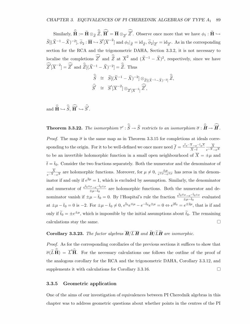
CHAPTER 3. EQUIVALENCES OF PI CHEREDNIK ALGEBRAS OF TYPE A1 89
Similarly, H := H ⊗Z
Z, H′ = H ⊗
Z′ Z′. Observe once more that we have φ1 : H →
S[(X−1−X)−2], φ2 : H → S′[X−2] and φ1|Z = id
Z, φ2|Z′ = id
Z′ . As in the corresponding
section for the RCA and the trigonometric DAHA, Section 3.3.2, it is not necessary to
localise the completions Z ′ and Z at X2 and (X−1 − X)2, respectively, since we have
Z′[X−2] = Z
′ and Z[(X−1 − X)−2] =
Z. Thus
S ∼= S[(X−1 − X)−2]⊗
Z[(X−1−X)−2]Z,
S′ ∼= S
′[X−2]⊗Z′[X
−2]Z′,
and H → S, H′ → S
′.
Theorem 3.3.22. The isomorphism τ ′ : S → S restricts to an isomorphism σ :
H→ H′.
Proof. The map σ is the same map as in Theorem 3.3.15 for completions at ideals corre-
sponding to the origin. For it to be well-defined we once more need f = ete−X−e−teX
X−tX
e−X−eX
to be an invertible holomorphic function in a small open neighbourhood of X = ±µ and
t = t0. Consider the two fractions separately. Both the numerator and the denominator ofX
e−X−eXare holomorphic functions. Moreover, for µ 6= 0, ±µ
e∓µ−e±µ has zeros in the denom-
inator if and only if e2µ = 1, which is excluded by assumption. Similarly, the denominator
and numerator of et0∓µ−e−t0±µ
±µ−t0are holomorphic functions. Both the numerator and de-
nominator vanish if ±µ− t0 = 0. By l’Hospital’s rule the fraction et0∓µ−e−t0±µ
±µ−t0evaluated
at ±µ− t0 = 0 is −2. For ±µ− t0 6= 0, et0e∓µ − e−t0e±µ = 0 ⇔ e2t0 = e±2µ, that is if and
only if t0 = ±e±µ, which is impossible by the initial assumptions about t0. The remaining
calculations stay the same.
Corollary 3.3.23. The factor algebras H/LH and H/LH are isomorphic.
Proof. As for the corresponding corollaries of the previous sections it suffices to show that
σ(L H) = L′H. For the necessary calculations one follows the outline of the proof of
the analogous corollary for the RCA and the trigonometric DAHA, Corollary 3.3.12, and
supplements it with calculations for Corollary 3.3.16.
3.3.5 Geometric application
One of the aims of our investigation of equivalences between PI Cherednik algebras in this
chapter was to address geometric questions about whether points in the centres of the PI
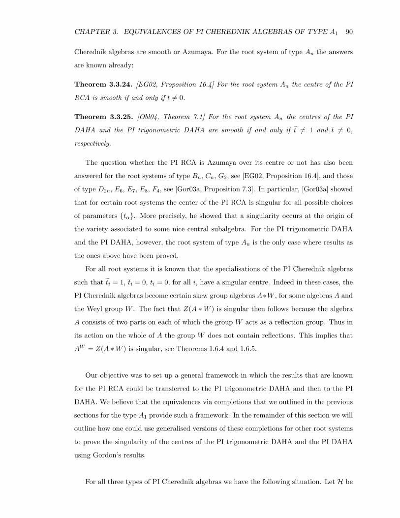
CHAPTER 3. EQUIVALENCES OF PI CHEREDNIK ALGEBRAS OF TYPE A1 90
Cherednik algebras are smooth or Azumaya. For the root system of type An the answers
are known already:
Theorem 3.3.24. [EG02, Proposition 16.4] For the root system An the centre of the PI
RCA is smooth if and only if t 6= 0.
Theorem 3.3.25. [Obl04, Theorem 7.1] For the root system An the centres of the PI
DAHA and the PI trigonometric DAHA are smooth if and only if t 6= 1 and t 6= 0,
respectively.
The question whether the PI RCA is Azumaya over its centre or not has also been
answered for the root systems of type Bn, Cn, G2, see [EG02, Proposition 16.4], and those
of type D2n, E6, E7, E8, F4, see [Gor03a, Proposition 7.3]. In particular, [Gor03a] showed
that for certain root systems the center of the PI RCA is singular for all possible choices
of parameters tα. More precisely, he showed that a singularity occurs at the origin of
the variety associated to some nice central subalgebra. For the PI trigonometric DAHA
and the PI DAHA, however, the root system of type An is the only case where results as
the ones above have been proved.
For all root systems it is known that the specialisations of the PI Cherednik algebras
such that ti = 1, ti = 0, ti = 0, for all i, have a singular centre. Indeed in these cases, the
PI Cherednik algebras become certain skew group algebras A∗W , for some algebras A and
the Weyl group W . The fact that Z(A ∗W ) is singular then follows because the algebra
A consists of two parts on each of which the group W acts as a reflection group. Thus in
its action on the whole of A the group W does not contain reflections. This implies that
AW = Z(A ∗W ) is singular, see Theorems 1.6.4 and 1.6.5.
Our objective was to set up a general framework in which the results that are known
for the PI RCA could be transferred to the PI trigonometric DAHA and then to the PI
DAHA. We believe that the equivalences via completions that we outlined in the previous
sections for the type A1 provide such a framework. In the remainder of this section we will
outline how one could use generalised versions of these completions for other root systems
to prove the singularity of the centres of the PI trigonometric DAHA and the PI DAHA
using Gordon’s results.
For all three types of PI Cherednik algebras we have the following situation. Let H be
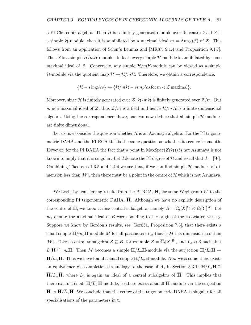
CHAPTER 3. EQUIVALENCES OF PI CHEREDNIK ALGEBRAS OF TYPE A1 91
a PI Cherednik algebra. Then H is a finitely generated module over its centre Z. If S is
a simple H-module, then it is annihilated by a maximal ideal m = AnnZ(S) of Z. This
follows from an application of Schur’s Lemma and [MR87, 9.1.4 and Proposition 9.1.7].
Thus S is a simple H/mH-module. In fact, every simple H-module is annihilated by some
maximal ideal of Z. Conversely, any simple H/mH-module can be viewed as a simple
H-module via the quotient map H → H/mH. Therefore, we obtain a correspondence:
H − simples ↔ H/mH− simples formC Zmaximal.
Moreover, since H is finitely generated over Z, H/mH is finitely generated over Z/m. But
m is a maximal ideal of Z, thus Z/m is a field and hence H/mH is a finite dimensional
algebra. Using the correspondence above, one can now deduce that all simple H-modules
are finite dimensional.
Let us now consider the question whetherH is an Azumaya algebra. For the PI trigono-
metric DAHA and the PI RCA this is the same question as whether its centre is smooth.
However, for the PI DAHA the fact that a point in MaxSpec(Z(H)) is not Azumaya is not
known to imply that it is singular. Let d denote the PI degree ofH and recall that d = |W |.
Combining Theorems 1.3.5 and 1.4.4 we see that, if we can find simple H-modules of di-
mension less than |W |, then there must be a point in the centre ofH which is not Azumaya.
We begin by transferring results from the PI RCA, H, for some Weyl group W to the
corresponding PI trigonometric DAHA, H. Although we have no explicit description of
the centre of H, we know a nice central subalgebra, namely B = Ct[X]W ⊗ Ct[Y ]W . Let
mo denote the maximal ideal of B corresponding to the origin of the associated variety.
Suppose we know by Gordon’s results, see [Gor03a, Proposition 7.3], that there exists a
small simple H/moH-module M for all parameters tα, that is M has dimension less than
|W |. Take a central subalgebra Z ⊆ B, for example Z = Ct[X]W , and Lo C Z such that
LoH ⊆ moH. Then M becomes a simple H/LoH-module via the surjection H/LoH
H/moH. Thus we have found a small simple H/LoH-module. Now we assume there exists
an equivalence via completions in analogy to the case of A1 in Section 3.3.1: H/LoH ∼=
H/LoH, where Lo is again an ideal of a central subalgebra of H. This implies that
there exists a small H/LoH-module, so there exists a small H-module via the surjection
H H/LoH. We conclude that the centre of the trigonometric DAHA is singular for all
specialisations of the parameters in t.
CHAPTER 3. EQUIVALENCES OF PI CHEREDNIK ALGEBRAS OF TYPE A1 92
Based on this result for the trigonometric DAHA one can then use isomorphisms be-
tween completions of the PI trigonometric DAHA and the PI DAHA, as in the case of A1
in Section 3.3.3, to deduce a similar statement for the DAHA.
Chapter 4
Graded Hecke algebras
In this last chapter we consider graded Hecke algebras. Our aim is to investigate under
which conditions these algebras satisfy a polynomial identity. After defining these alge-
bras and describing some of their properties in Section 4.1, we use deformation theory
to motivate and justify this in Section 4.2. The spherical subalgebra of a graded Hecke
algebra plays a crucial role in proving our main theorem and we examine it in Section 4.3.
In Section 4.4 we give details of some preliminary results. Finally, we prove the main the-
orem in Section 4.5. This theorem tells us for which values of the deformation parameters
graded Hecke algebras have a big centre. As a corollary we deduce that the graded Hecke
algebras are PI algebras for these values.
4.1 Definition and first properties
Let V be a finite dimensional vector space over C and G a finite subgroup of GL(V ).
Denote by κ : V × V → CG a skew-symmetric bilinear form. Let
T (V ) = C⊕ V ⊕ (V ⊗ V )⊕ · · ·
be the tensor algebra of V . The action of G on V extends to an action of G on T (V )
by C-algebra automorphisms. We construct the skew group algebra T (V ) ∗ G, compare
Section 1.6, and then define a factor algebra of this skew group algebra by
A :=(T (V ) ∗G
)/〈[v, w]− κ(v, w) : v, w ∈ V 〉,
where [v, w] = vw − wv.
The algebra A is a positively filtered algebra. Namely let F 0A be the image of CG under
the projection T (V )∗G→ A. Let F 1A be the image of CG+CGV under this projection and
93
CHAPTER 4. GRADED HECKE ALGEBRAS 94
F iA = (F 1A)i for i > 1. We form the associated graded algebra of A under this filtration,
grA. From the relations in A it is clear that there exists an epimorphism S(V )∗G grA.
Here S(V ) denotes the symmetric algebra of V , that is S(V ) = T (V )/〈vw−wv : v, w ∈ V 〉.
Definition 4.1.1. [RS03, Section 1] The algebra A is called a graded Hecke algebra if
S(V ) ∗G ∼= grA.
This means that a graded Hecke algebra A is isomorphic to S(V ) ⊗ CG as a graded
vector space, which provides us with a PBW basis for A.
The next step is to give a more precise description of the form κ that appears in the
definition of the algebra A. The PBW basis for the graded Hecke algebra A imposes
necessary conditions on the form κ. For example, we deduce that κ is G-invariant in
the sense that gκ(v, w)g−1 = κ(g(v), g(w)), because otherwise there exists a nontrivial
linear relation in A between elements of CG. This follows because of the relation gvg−1 =
g(v), for all g ∈ G and v ∈ V , in the skew group algebra T (V ) ∗ G, which implies that
g(vw − wv)g−1 = g(v)g(w) − g(w)g(v) for all v, w ∈ V . In fact, the choices for the form
κ that can be used to construct a graded Hecke algebra are rather restricted. In order to
describe these choices we need to introduce more notation.
Denote the centraliser of an element g ∈ G by ZG(g). Recall that a bireflection in G is
an element s 6= id ∈ G that fixes a subspace of V of codimension 2, that is rankV (id−s) =
2. Write V s = ker(id − s) for the subspace of V fixed by s. Note that for g ∈ ZG(s),
we have g(V s) = V s. Then we define the set S to be a subset of the set of bireflections,
namely S is the set of bireflections s such that the following condition holds:
∀g ∈ ZG(s), det(g|V/V s) = 1. (4.1)
This set is closed under conjugation. Indeed for g ∈ G, s ∈ S, rankV (id − g−1sg) =
rankV (g−1(id − s)g) = rankV (id − s) = 2. Moreover, ZG(g−1sg) = g−1ZG(s)g. Say
h ∈ ZG(g−1sg), then h = g−1h′g, for some h′ ∈ ZG(s). It is easy to see that V ∼= V s⊕V/V s,
since V s = ker(id − s) and V/V s ∼= im(id − s). Thus choose a basis for the subspace V s
and extend it to a basis for all of V . Now perform a change of basis by conjugating
with the matrix corresponding to g ∈ G. The subspace V s is mapped by this base
change to the subspace V g−1sg, and the matrix of h′ with respect to the original basis
becomes the matrix of g−1h′g with respect to the new basis. Since h′ ∈ ZG(s) and s ∈ S,
CHAPTER 4. GRADED HECKE ALGEBRAS 95
det(h′|V/V s) = 1 and, therefore, det((g−1h′g)|V/V g−1sg) = 1. Hence condition (4.1) is
satisfied by all h ∈ ZG(g−1sg).
Let us construct specific skew-symmetric bilinear forms on V as follows. Fix s ∈ S.
Since s is a bireflection, the space im(id−s) is two-dimensional. Up to scalar multiplication
there is a unique nonzero skew-symmetric bilinear form on im(id− s). We can extend this
form to all of V by setting V s = ker(id− s) to be its radical. Denote the form constructed
in this way by Ωs. Using this form as a starting point we can define new forms: for g ∈ G
and v, w ∈ V ,
Ωg−1sg(v, w) := Ωs(g(v), g(w)).
With some easy calculations one can check that the form Ωg−1sg defined in this way is
indeed a nonzero skew-symmetric bilinear form on im(id− g−1sg) and that the radical of
Ωg−1sg is ker(id− g−1sg). Thus for a fixed element s ∈ S the forms corresponding to the
elements in the conjugacy class of s are determined by Ωs.
Finally, let Ω be any skew-symmetric bilinear form on V , which is G-invariant, that is
Ω ∈ ((∧2 V )∗)G. The space ((
∧2 V )∗)G is a finite dimensional vector space over C. Let
b1, . . . , bN denote a basis for ((∧2 V )∗)G over C. Then Ω =
∑Ni=1 qibi for some qi ∈ C.
Now we are ready to state the crucial result:
Theorem 4.1.2. [Dri86, Section 4], [RS03, Theorem 1.9] With the above notation the
algebra A is a graded Hecke algebra if and only if, for all v, w ∈ V ,
κ(v, w) = Ω(v, w) id+∑s∈S
csΩs(v, w) s,
where Ω(v, w) =∑N
i=1 qibi(v, w) for some qi ∈ C, and the map c : S → C given by s 7→ cs
is invariant under conjugation by G.
Therefore, graded Hecke algebras are determined by the choice of the complex values for
qi | i = 1 . . . , N and cs | s ∈ S. Henceforth we let q denote the N -tuple of parameters
qi and c denote the tuple of parameters cs | s ∈ S. Moreover, we will indicate through
notation if we choose particular complex numbers for these parameters. However, it will
not be necessary to consider the parameters in q and c as variables and the definition of
a graded Hecke algebra over C[q, c] as we did for the Cherednik algebras in the previous
chapters.
CHAPTER 4. GRADED HECKE ALGEBRAS 96
A justification for the particular form of κ that appears in this theorem will be given
in the following section.
If qi = 0 for all i = 1, . . . , N and cs = 0 for all s ∈ S, then A(q=0,c=0) = S(V ) ∗ G.
This follows directly from the defining relations of A. This fact explains why one speaks
of the graded Hecke algebra as a deformation of the skew group algebra S(V ) ∗G.
Remark 4.1.3. Let us briefly comment on the fact that symplectic reflection algebras
(SRAs) appear as special cases of graded Hecke algebras. Suppose the vector space V
is a symplectic vector space, thus there exists a non-degenerate skew-symmetric bilinear
form ω on V . Furthermore suppose that the group G preserves this form, which means
that ω(g(v), g(w)) = ω(v, w) for all g ∈ G and v, w ∈ V . In the study of SRAs one can
reduce to the case where V contains no non-degenerate G-invariant subspaces. Under
this assumption it can be shown that ((∧2 V )∗)G = Cω, see [EG02, Section 2, p. 256].
Thus without loss of generality we set Ω = ω. Take a bireflection s. Then we saw that
V = ker(id− s)⊕ im(id− s). This decomposition is in fact ω-orthogonal. Namely, assume
that s acts diagonally on V and that w ∈ V is such that s(w) = λw for some λ 6= 1 in C∗.
Furthermore, let v ∈ ker(id− s), that is s(v) = v. Then
ω(v, w) = ω(s(v), w) = ω(v, s−1(w)) = λ−1ω(v, w).
Now we combine this with the fact that ω is non-degenerate on V to deduce that ω|im(id−s)
is non-degenerate. Without loss of generality we can, therefore, assume that ω|im(id−s) =
Ωs. Since G preserves the symplectic form ω, every bireflection in G automatically
fulfills condition (4.1). Namely, let v1, v2 denote a basis of V/V s ∼= im(id − s). For
g ∈ ZG(s) we have g(v1) = av1 + bv2 and g(v2) = cv1 + dv2 for some a, b, c, d ∈ C.
Then ω|im(id−s)(v1, v2) = ω|im(id−s)(g(v1), g(v2)) = (ad − bc)ω|im(id−s)(v1, v2) implies that
ad − bc = 1, which is condition (4.1). We have arrived at the definition of an SRA,
see [EG02, Theorem 1.3].
Denote the subgroup of G generated by the subset S by S.
Remark 4.1.4. The subgroup S does not contain reflections. This follows directly from
the fact that S is in fact a subgroup of SL(V ). To see the latter take a generator s of S.
Then s ∈ ZG(s) and thus det(s|V/V s) = 1 by condition (4.1). But V = V s ⊕ V/V s and
det(s|V s) = 1 by construction. Hence, det(s) = det(s|V/V s) · det(s|V s) = 1.
CHAPTER 4. GRADED HECKE ALGEBRAS 97
Proposition 4.1.5. Let A be a graded Hecke algebra.
(i) A = A(S) ∗′ (G/S), where A(S) denotes the graded Hecke algebra corresponding to
S instead of G, and ∗′ denotes some crossed product.
(ii) For λ ∈ C∗, let Aλ denote the graded Hecke algebra
Aλ :=(T (V ) ∗G
)/〈[v, w]− λκ(v, w) : v, w ∈ V 〉.
Then Aλ ∼= A.
Proof. (i) We observed before that the subset S of G is closed under conjugation by G.
Thus the subgroup S generated by S is a normal subgroup of G. Denote the ideal of
T (V ) ∗G generated by
[v, w] = κ(v, w) = Ω(v, w)id+∑s∈S
csΩs(v, w)s,
for all v, w ∈ V , by I. Then A = (T (V ) ∗ G)/I by definition. By [Pas89, Lemma 1.3],
(T (V ) ∗G)/I =[(T (V ) ∗ S) ∗′ (G/S)
]/I. Indeed T (V ) ∗ S is just the sub-skew group ring
of T (V ) ∗ G. So an element x ∈ T (V ) ∗ S can be written uniquely as x =∑
s∈S xss for
some xs ∈ T (V ). Since S is a normal subgroup of G, the conjugation action of G on S
induces an automorphism of CS. Let g denote an element in G/S and g ∈ G an inverse
image of g. Multiplication in (T (V )∗S)∗′G/S is determined by the rule g ·x = g(x) ·g and
g(x) =∑
s∈S g(xs) ·g−1sg. Since κ(v, w) ∈ CS, for all v, w ∈ V , the generators of the ideal
I also generate an ideal of T (V ) ∗S, which we denote by IS . We have I = IS(T (V ) ∗G) =
(T (V )∗G)IS and A =[(T (V )∗S)∗′ (G/S)
]/I =
[(T (V )∗S)/IS
]∗′ (G/S) = A(S)∗′ (G/S).
(ii) Define a map A→ Aλ by x 7→√λx and g 7→ g for x ∈ T (V ), g ∈ G.
Because of the close connection between A and A(S) - as exhibited in this proposition
- we will often restrict ourselves to the case when G is generated by the elements of S that
it contains, hence to the case G = S.
We saw that A is a filtered algebra. This allows us to use associated graded techniques
to deduce properties of A from properties of its associated graded algebra, grA ∼= S(V )∗G.
Proposition 4.1.6. Let A be a graded Hecke algebra. Then A is noetherian, prime and
has finite global dimension.
Proof. By Theorem 1.2.4 all of these properties follow if one can show that they hold for
S(V ) ∗ G. But this can be deduced from Theorem 1.6.1 and basic properties of S(V ) =
C[V ∗].
CHAPTER 4. GRADED HECKE ALGEBRAS 98
4.2 PBW deformation
In this section we want to explain how the graded Hecke algebras A are precisely the PBW
deformations of the skew group algebra R := S(V ) ∗G of a certain kind. This will justify
the particular shape that the skew-symmetric bilinear form κ : V × V → CG takes in
Theorem 4.1.2. To do this we first recall some deformation theory.
The algebra R = S(V ) ∗ G is naturally a positively graded algebra with degCG = 0
and the n-th graded piece of S(V ) denoted by Sn(V ). Let Ri be the ith graded part
of the algebra R so that Ri = Si(V )G = GSi(V ), and thus each graded part Ri is a
CG-bimodule. Then R can be viewed as a graded CG-bimodule and the multiplication
in R gives a CG-bimodule map R ⊗CG R → R. From investigating the relations in A it
is clear that - when deforming R into A - we do not want to deform the relations in the
group algebra CG. Therefore, to ensure that we do not deform the degree zero part of the
algebra R we will use the following definition in this section and only in this section:
Definition 4.2.1. Let B be a CG-bimodule with a CG-bimodule map B ⊗CG B → B.
Then we call B a CG-algebra.
All the maps that occur subsequently in the deformation of R will be assumed to be
CG-bimodule maps and we will frequently tensor over CG instead of C, which we will
clarify by notation. In the literature deformation theory is usually defined for algebras
over a field, but, as mentioned in [EG02, Section 2, p. 256], the theory explained in this
section and in particular the results of [BG96] also hold for CG-algebras as defined above.
We recall the definition of a graded deformation of R. Let C[h] denote the polynomial
ring in one variable and set degh = 1. Suppose Rh is an associative unital algebra such that
the underlying C-vector space of Rh is R⊗C[h]. Then (Rh, ∗) is a graded deformation of R
if the multiplication ∗ : Rh×Rh → Rh is a C[h]-linear map such that r1∗r2 ≡ r1r2 modhRh,
for all r1, r2 ∈ R. Thus R = Rh/hRh. In this document we also require that Rh is a graded
CG[h]-bimodule and that ∗ is a CG[h]-bimodule map, so that Rh is also a CG-algebra.
If Rh is a graded deformation of R, then the multiplication of two elements r1, r2 ∈ R
can be described by
r1 ∗ r2 = r1r2 + µ1(r1, r2) · h+ µ2(r1, r2) · h2 + · · · .
CHAPTER 4. GRADED HECKE ALGEBRAS 99
The term r1r2 denotes the product in R and the maps µi : R ×R→ R are CG-bimodule
maps of degree −i with i ∈ N. The latter means that µi : Rj ×Rk → Rk+j−i. These maps
determine the multiplication in Rh because of CG[h]-linearity. Moreover, the fact that Rh
is an associative algebra with a unit imposes certain conditions on the bimodule maps µi.
We will provide a more detailed account of this in the next lemma. For example, one can
deduce that µ(g, r) = gµ(1, r) = 0 and µ(r, g) = µ(r, 1)g = 0, for all g ∈ CG and r ∈ R.
Thus the multiplication in CG ⊂ R is not deformed.
An ith level deformation is defined as above with the truncated polynomial ring
Rh/hi+1Rh instead of Rh. A first level deformation is called an infinitesimal deforma-
tion.
Remark 4.2.2. Graded deformations have the following property: for all λ ∈ C the factor
Rh,λ := Rh/(h − λ)Rh is a filtered algebra such that there is a canonical isomorphism
grRh,λ ∼= R as algebras and also as CG-algebras. The filtration on Rh,λ is induced by
the filtration on Rh, which in turn is derived from the grading on Rh. Namely, F iRh,λ=
F iRh/(F iRh
∩(h−λ)Rh)
= F iRh/(h−λ)F i−1
Rh, where F iRh
is the filtration on Rh. Take the map
ϕ : F iRh,λ→ F iRh
/(F i−1Rh
+hF i−1Rh
), for all i ≥ 0, given by r+(h−λ)F i−1
Rh7→ r+F i−1
Rh+hF i−1
Rh,
for all r ∈ F iRh. The expression on the right hand side of the map is just the i-th graded
piece of R. It is routine to check that this is a well-defined C-algebra map and also a CG-
bimodule map. Furthermore, the kernel of ϕ is clearly F i−1Rh,λ
and so ϕ gives the required
isomorphism.
There is a strong connection between graded deformations of the CG-algebra R and its
graded Hochschild cohomology groups. Very briefly, see [BG96, Section 2], the Hochschild
cohomology of R with coefficients in a graded R-bimodule M , is the cohomology of the
following complex
· · · ∂p−1
−−−→ Homgr(TpCG(R),M) ∂p
−→ Homgr(Tp+1CG (R),M) ∂p+1
−−−→ · · · . (4.2)
Since we are considering R as a CG-algebra, we use T pCG(R), the tensor product of p copies
of R over CG, and Homgr(TpCG(R),M), the set of graded R-bimodule homomorphisms from
T pCG(R) to M . The differential is given by
∂p(f)(x1, . . . , xp+1) = x1f(x2, . . . , xp+1) +p∑
m=1
(−1)mf(x1, . . . , xmxm+1, . . . , xp+1)
+(−1)p+1f(x1, . . . , xp)xp+1,
for f ∈ Homgr(TpCG(R),M). Hence, the Hochschild cohomology is given by Hk(R,M) :=
CHAPTER 4. GRADED HECKE ALGEBRAS 100
ker∂k/im∂k−1, k ∈ N. Observe that these cohomology groups inherit a direct sum
decomposition into graded pieces: Hk(R,M) =⊕
i∈ZHki (R,M), where the degree of
Hki (R,M) comes from the degree of the cocycles, thus the degree of the elements in
ker∂k ⊆ Homgr(T kCG(R),M).
Lemma 4.2.3. [BG96, Proposition 1.5] The set of isomorphism classes of infinitesimal
deformations of R canonically identifies with H2−1(R,R).
Let us explain the statement of this lemma. On the one hand we have H2−1(R,R) =
(ker∂2)−1/(im∂1)−1, where (ker∂2)−1 denotes the maps of degree −1 in ker∂2 and similarly
for (im∂1)−1. On the other hand, infinitesimal deformations are of the form (Rh/h2Rh, ∗),
where Rh/h2Rh is an associative C-algebra and a graded CG[h]-bimodule. The multi-
plication ∗ of elements r1, r2 ∈ R is given by r1 ∗ r2 = r1r2 + µ1(r1, r2) · h. Thus the
CG-bimodule map µ1 of degree −1 completely determines the infinitesimal deformation
by CG[h]-linearity. The only condition for the multiplication ∗ to be a CG[h]-bimodule
map and for Rh/h2Rh to be an algebra is associativity. But ∗ is completely determined
by its action on elements of R by CG[h]-linearity. For r1, r2, r3 ∈ R, the condition
(r1 ∗ r2) ∗ r3 = r1 ∗ (r2 ∗ r3) translates into
r1µ1(r2, r3)− µ1(r1r2, r3) + µ1(r1, r2r3)− µ1(r1, r2)r3 = 0.
Now µ1 ∈ Hom−1(T 2CG(R), R), where Hom−1(T 2
CG(R), R) denotes the graded homomor-
phisms of degree −1. Thus, if we compare above equation with the definition of the
differential ∂ in the complex (4.2), then we see that the equation is equivalent to saying
∂2(µ1)(r1, r2, r3) = 0, that is µ1 ∈ (ker∂2)−1.
Suppose that we are given two isomorphic infinitesimal deformations (Rh/h2Rh, ∗) and
(Rh/h2Rh, ∗′). Then there exists a CG-bimodule map g : Rh/h2Rh → Rh/h2Rh such that
g = id mod hRh and g(p1 ∗ p2) = g(p1) ∗′ g(p2) for all p1, p2 ∈ Rh/h2Rh. For r ∈ R we can
write g(r) = r + g1(r)h for some CG-linear map g1 : R → R of degree −1 and this map
g1 again determines the map g completely by CG[h]-linearity. For elements r1, r2 ∈ R the
condition g(r1 ∗ r2) = g(r1) ∗′ g(r2) translates into
µ1(r1, r2) + g1(r1r2) = µ′1(r1, r2) + g1(r1)r2 + r1g1(r2).
But g1 ∈ Hom(T 1CG(R), R), and the above equation says that (µ1−µ′1)(r1, r2) = g1(r1)r2 +
r1g1(r2)− g1(r1r2), that is µ1 − µ′1 = ∂1(g1) and so µ1 − µ′1 ∈ im∂1.
CHAPTER 4. GRADED HECKE ALGEBRAS 101
Moreover, it can be shown that the obstructions to constructing higher level graded
deformations - starting from the infinitesimal deformation - lie in higher graded Hochschild
cohomology groups, see [BG96, Proposition 1.5]. Therefore, if the higher graded Hochschild
cohomology groups of R with coefficients in R vanish, then the deformation theory of R
is particularly nice. In [BG96, Definition 3.4] it is shown that for a Koszul algebra B all
relevant higher graded Hochschild cohomology groups of B with coefficients in B vanish.
This result can be adjusted to the case where B is also a CG-algebra. As it turns out,
the algebra R = S(V ) ∗G is a Koszul algebra. Let us define the last term and justify this
claim. Some details are taken from [Gor05].
Definition 4.2.4. [BGS96, Definition 1.1.2] Let B =⊕∞
i=0Bi be a positively graded ring
such that B0 is semi-simple. Then B is Koszul if B0 = B/B>0 considered as a graded left
B-module admits a graded projective resolution
· · · → P 2 → P 1 → P 0 → B0 → 0
such that the maps P j → P j−1 are graded of degree zero and P j is generated by its degree
j component.
In [BG96, Definition 3.4, Claim 3.6 and Appendix] a number of equivalent definitions
of a Koszul algebra are given.
To see that R is a Koszul algebra we consider the following resolution of R0 = CG:
· · · → S(V )⊗C
p∧V ⊗C CG→ · · · → S(V )⊗C
1∧V ⊗C CG→ S(V )⊗C CG→ CG→ 0,
(4.3)
where the differential d : S(V )⊗C∧p V ⊗C CG→ S(V )⊗C
∧p−1 V ⊗C CG is given by
d(x⊗ vi1 ∧ · · · ∧ vip ⊗ g) =p∑j=1
(−1)j−1xvij ⊗ vi1 ∧ · · · ∧ vij ∧ · · · ∧ vip ⊗ g,
for x ∈ S(V ), vi1 , . . . , vip ∈ V , g ∈ CG. First we observe that each of the vector spaces
S(V ) ⊗C∧p V ⊗C CG is indeed a left R-module: the action of y ⊗ g′ ∈ R, y ∈ S(V ),
g′ ∈ CG on x⊗ vi1 ∧ · · · ∧ vip ⊗ g is given by
(y ⊗ g′)(x⊗ vi1 ∧ · · · ∧ vip ⊗ g) = yg′(x)⊗ g′(vi1) ∧ . . . ∧ g′(vip)⊗ g′g.
It is easy to check that
(y ⊗ g′)(x⊗ vi1 ∧ · · · ∧ vip ⊗ g) = (g′ ⊗ (g′)−1(y))(x⊗ vi1 ∧ · · · ∧ vip ⊗ g)
CHAPTER 4. GRADED HECKE ALGEBRAS 102
and that the differentials d in (4.3) are R-module maps. Moreover, we claim that the left
R-modules S(V )⊗C∧p V ⊗C CG are free for all p ≥ 1. First note that
∧p V ⊗C CG is a
free left CG-module, see [Pas77, Lemma 10.3.5]. A basis for∧p V ⊗C CG as CG-module
is given by the C-basis of∧p V . Denote this basis by fii≥1. Then one can check that
1⊗fii≥1 is a basis for S(V )⊗C∧p V ⊗C CG as left R-module. Finally, the complex (4.3)
is a resolution, since it is simply the Koszul resolution of C as S(V )-module tensored on
the right by CG, see [BGS96, Remark (2) in Section 1.2]. We conclude that the complex
(4.3) is a free R-module resolution of R0 = CG.
Furthermore, note that the R-modules S(V )⊗C∧p V ⊗CCG are graded. Namely, we set
the degree of g ∈ CG to be zero, the degree of v ∈ V to be one and deg(vi1 ∧ · · ·∧ vip) = p.
Clearly, the differentials are homogeneous of degree zero. The last thing we need to show is
that each vector space S(V )⊗C∧p V ⊗C CG is generated as R-module by its degree p part,∧p V . But this is our earlier observation about the R-module basis of S(V )⊗C
∧p V ⊗CCG.
In the following we will use the concept of a quadratic CG-algebra and the fact that
the CG-algebra R has this property. For a definition of a quadratic algebra over a field
see [BG96, 0.1 and 0.2]. In our case let E denote some CG-bimodule and let TCG(E) denote
the tensor CG-algebra. Let P be a subset of CG⊕E⊕(E⊗CGE) and also a CG-bimodule.
If we denote the ideal generated by P by I(P ), then the algebra Q(E,P ) = TCG(E)/I(P )
is called a nonhomogeneous quadratic CG-algebra. If D is a subset of E ⊗CG E and also a
CG-bimodule, then the algebra Q(E,D) = TCG(E)/I(D) is called a quadratic CG-algebra.
Observe that we can assume that D and P are CG-bimodules without loss of generality,
because ifD and P are arbitrary subsets we can take the CG-bimodules that they generate.
Next we show that R is a quadratic CG-algebra, see also [EG02, p. 256]. Some details
are taken again from [Gor05]. Take E := V ⊗C CG and observe that E is a free CG module
on the right by multiplication and a free CG-module on the left by g(v⊗g′) = g(v)⊗g ·g′,
for v ∈ V and g, g′ ∈ CG, see [Pas77, Lemma 10.3.5]. Let D ⊆ E ⊗CG E be the C-span of
(v ⊗ 1)⊗CG (w ⊗ g)− (w ⊗ 1)⊗CG (v ⊗ g),
for v, w ∈ V and g ∈ CG. Note that D is a CG-bimodule with the actions
g′[(v ⊗ 1)⊗CG (w ⊗ g)− (w ⊗ 1)⊗CG (v ⊗ g)] =
(g′(v)⊗ 1)⊗CG (g′(w)⊗ g′g)− (g′(w)⊗ 1)⊗CG (g′(v)⊗ g′g),
CHAPTER 4. GRADED HECKE ALGEBRAS 103
[(v⊗1)⊗CG (w⊗g)− (w⊗1)⊗CG (v⊗g)]g′ = (v⊗1)⊗CG (w⊗gg′)− (w⊗1)⊗CG (v⊗gg′),
for g′ ∈ CG. The crucial step to seeing that S(V ) ∗G ∼= Q(E,D) as CG-algebras is that
TCG(E) ∼= T (V ) ∗ G as CG-algebras, where T (V ) denotes the usual tensor algebra of V
over C. The last isomorphism, denoted by θ, is the direct sum of the following maps:
θp : E⊗CGp → V ⊗p ⊗ CG, given by
θp[(v1 ⊗ g1)⊗CG · · · ⊗CG (vp ⊗ gp)] =(v1 ⊗ h1(v2)⊗ h2(v3)⊗ · · · ⊗ hp−1(vp)
)⊗ hp,
where vi ∈ V , gi ∈ CG and hi := g1 · · · gi for i = 1, . . . , p. Then
θ2(D) = C− span(v1 ⊗ v2 − v2 ⊗ v1)⊗ g, v1, v2 ∈ V, g ∈ CG = C ⊗ CG,
where C denotes the space of commutators in V ⊗2. Thus TCG(E)/I(D) ∼= S(V ) ∗G.
We are now almost in the position to define a PBW deformation. Suppose we have a
nonhomogeneous quadratic CG-algebra Q(E,P ). Then there exists a canonical quadratic
CG-algebra Q(E,D) associated to Q(E,P ), namely define π : CG ⊕ E ⊕ (E ⊗CG E) 7→
E ⊗CG E to be the projection map and set D = π(P ). Note that Q(E,P ) is filtered as
follows. The CG-algebra TCG(E) has a natural grading, where CG is in degree zero and
degE = 1. Thus we have a filtration F •TCG(E) on TCG(E) given by F iTCG(E) =⊕i
j=0 TjCG(E),
where T jCG(E) denotes the j-th graded piece of TCG(E). Let p : TCG(E) Q(E,P ) be
the natural surjection. Then setting F iQ(E,P ) := p (F iTCG(E)) = F iTCG(E)/(F iTCG(E) ∩ I(P )
)induces a filtration on Q(E,P ). Let grQ(E,P ) denote the associated graded CG-algebra
of Q(E,P ) under this filtration. By construction grQ(E,P ) is generated by p(E) over CG.
Thus there exists a surjective CG-algebra map TCG(E) grQ(E,P ). By the construction
of P such that π(P ) = D we even have ψ : Q(E,D) grQ(E,P ).
Definition 4.2.5. [BG96, Definition 0.3] The nonhomogeneous quadratic CG-algebra
Q(E,P ) is called a PBW deformation of Q(E,D) if ψ is an isomorphism, that is if
Q(E,D) ∼= grQ(E,P ).
It is clear that any PBW deformation Q(E,P ) of Q(E,D) must satisfy the condition
P ∩ F 1TCG(E) = 0. (4.4)
If this condition holds, the CG-bimodule P can be written uniquely in terms of two CG-
bimodule maps α : D 7→ E and β : D 7→ CG as P = d− α(d)− β(d) : d ∈ D.
CHAPTER 4. GRADED HECKE ALGEBRAS 104
We have already seen that the algebra R = S(V ) ∗G is a quadratic CG-algebra with
E := V ⊗C CG and D ⊆ E ⊗CG E being the C-span of
(v ⊗ 1)⊗CG (w ⊗ g)− (w ⊗ 1)⊗CG (v ⊗ g),
for v, w ∈ V and g ∈ CG. Let us now show how the graded Hecke algebras that we defined
in the previous section fit into this picture.
Lemma 4.2.6. Let A be a graded Hecke algebra and let Q(E,D) ∼= S(V ) ∗ G, with E
and D defined as above. Then A is a nonhomogeneous quadratic CG-algebra Q(E,P ) with
P ⊆ CG⊕E⊕ (E⊗CGE) such that the quadratic CG-algebra associated to Q(E,P ) under
the projection π : CG⊕E ⊕ (E ⊗CG E) 7→ E ⊗CG E is S(V ) ∗G ∼= Q(E,D). Thus A is a
PBW deformation of S(V ) ∗G as defined in Definition 4.2.5.
Proof. A graded Hecke algebra is of the form A = (T (V )∗G)/I, where I denotes the ideal
generated by
[v1, v2]− κ(v1, v2),
for all v1, v2 ∈ V , see Theorem 4.1.2. Equivalently one could choose as generators of the
ideal I the elements([v1, v2]−κ(v1, v2)
)g, for all v1, v2 ∈ V and g ∈ CG. We have seen on
the previous page that TCG(E) ∼= T (V ) ∗G via an isomorphism which we labelled θ. The
map θ induces an isomorphism A ∼= TCG(E)/I(P ), where P is the C-span of
(v1 ⊗ 1)⊗CG (v2 ⊗ g)− (v2 ⊗ 1)⊗CG (v1 ⊗ g)− κ(v1, v2)g,
for v1, v2 ∈ V, g ∈ CG. Then P is clearly a subset of CG ⊕ E ⊕ (E ⊗CG E) and also a
CG-bimodule with the actions
g′[(v ⊗ 1)⊗CG (w ⊗ g)− (w ⊗ 1)⊗CG (v ⊗ g)− κ(v1, v2)g] =
(g′(v)⊗ 1)⊗CG (g′(w)⊗ g′g)− (g′(w)⊗ 1)⊗CG (g′(v)⊗ g′g)− κ(g′(v1), g′(v2))g′g,
[(v ⊗ 1)⊗CG (w ⊗ g)− (w ⊗ 1)⊗CG (v ⊗ g)− κ(v1, v2)g]g′ =
(v ⊗ 1)⊗CG (w ⊗ gg′)− (w ⊗ 1)⊗CG (v ⊗ gg′)− κ(v1, v2)gg′,
since g′κ(v1, v2) = κ(g′(v1), g′(v2))g′ by the G-invariance of the form κ. The image of P
under the projection π : CG ⊕ E ⊕ (E ⊗CG E) 7→ E ⊗CG E is precisely D. Thus A is a
nonhomogeneous quadratic algebra of the form Q(E,P ) such that π(P ) = D. By defini-
tion, grA ∼= S(V ) ∗G, which means that graded Hecke algebras are PBW deformations of
S(V ) ∗G.
CHAPTER 4. GRADED HECKE ALGEBRAS 105
Since A is a PBW deformation of Q(E,D) ∼= S(V ) ∗G, it must satisfy condition (4.4),
which implies that we can write P in terms of CG-bimodule maps α and β. An inspection
of the relations in Amakes it clear that β[(v⊗1)⊗CG(w⊗g)−(w⊗1)⊗CG(v⊗g)] = κ(v, w)g
and α = 0 will do.
We now want to show that, conversely, all PBW deformations of S(V ) ∗ G with a
certain property are graded Hecke algebras. We have the following result
Theorem 4.2.7. [BG96, Lemma 0.4, Lemma 3.3, Theorem 4.1] Let Q(E,D) be a quadratic
Koszul CG-algebra, where E is a free CG-module from either side. Assume that we
are given Q(E,P ) in terms of CG-bimodule maps α : D 7→ E, β : D 7→ CG, and
P = d − α(d) − β(d) : d ∈ D. Then Q(E,D) 7→ grQ(E,P ) is an isomorphism if
and only if the following are satisfied:
(i) α⊗CG id− id⊗CG α has image in D;
(ii) α (α⊗CG id− id⊗CG α) = id⊗CG β − β ⊗CG id;
(iii) β (α⊗CG id− id⊗CG α) = 0;
where the domain of all these maps is (D ⊗CG E) ∩ (E ⊗CG D).
Remark 4.2.8. In fact, in [BG96, Theorem 4.1] it is proved that the conditions (i) - (iii)
on the maps α and β and the fact that Q(E,D) is Koszul allow one to construct a graded
deformation (Q(E,D)h, ∗). Let Q(E,D)h,1 = Q(E,D)h/((h − 1)Q(E,D)h
). One then
obtains CG-bimodule maps
Q(E,D)ψ−→ grQ(E,P )
ρ−→ grQ(E,D)h,1ϕ−→ Q(E,D),
where we have seen before that ψ is a surjection and, by Remark 4.2.2 in this section, that
ϕ is an isomorphism. The map ρ comes from the CG-bimodule map that includes E in
Q(E,D)h and then projects onto Q(E,D)h,1. This map extends uniquely to an algebra
and CG-bimodule map TCG(E) → Q(E,D)h,1, which factors through Q(E,P ). The map
ρ is then the associated graded map of this map Q(E,P ) → Q(E,D)h,1. Finally, one
checks that the composition ϕ ρ ψ is the identity map on elements of degrees zero and
one in Q(E,D). Since Q(E,D) is generated by those elements, the composition is just the
identity map which implies grQ(E,P ) ∼= grQ(E,D)h,1 and Q(E,D) ∼= grQ(E,P ).
Corollary 4.2.9. Let Q(E,D) ∼= S(V ) ∗G, with E and D as before. Suppose Q(E,P ) is
a nonhomogeneous quadratic CG-algebra and a PBW deformation of Q(E,D) ∼= S(V )∗G.
Then the CG-bimodule P is given by CG-bimodule maps α : D 7→ E and β : D 7→ CG,
CHAPTER 4. GRADED HECKE ALGEBRAS 106
such that P = d− α(d)− β(d) : d ∈ D. Assume that α = 0. Then Q(E,P ) is a graded
Hecke algebra.
Proof. The details are taken from [EG02, p.257] and [Gor05] and are listed here for the
reader’s convenience.
We are given Q(E,D) ∼= S(V ) ∗ G so that E = V ⊗C CG and D ⊆ E ⊗CG E is
the CG-bimodule defined before. Furthermore, Q(E,P ) is a nonhomogeneous quadratic
CG-algebra with a CG-bimodule map β : D → CG such that P = d − β(d) : d ∈
D, π(P ) = D and Q(E,D) ∼= grQ(E,P ). Since β is a right CG-module map, it is
determined by its action on (v ⊗ 1) ⊗CG (w ⊗ 1) − (w ⊗ 1) ⊗CG (v ⊗ 1). Thus β is
determined by an antisymmetric mapping V × V → CG. Denote this map by κ, then
β[(v ⊗ 1)⊗CG (w ⊗ 1)− (w ⊗ 1)⊗CG (v ⊗ 1)] = κ(v, w). On the left we have
β[g((v ⊗ 1)⊗CG (w ⊗ 1)− (w ⊗ 1)⊗CG (v ⊗ 1)
)]=
β[(g(v)⊗ 1)⊗CG (g(w)⊗ g)− (g(w)⊗ 1)⊗CG (g(v)⊗ g)
]=
gβ[(v ⊗ 1)⊗CG (w ⊗ 1)− (w ⊗ 1)⊗CG (v ⊗ 1)
],
which translates in terms of the map κ into κ(g(v), g(w))g = gκ(v, w) or κ(g(v), g(w)) =
gκ(v, w)g−1. Since Q(E,P ) is a PBW deformation of Q(E,D) the map β must satisfy
conditions (i) - (iii) of the previous theorem. But only condition (ii) is nontrivial. It
reduces to 0 = id⊗CG β − β ⊗CG id on (D⊗CG E)∩ (E ⊗CGD). As we mentioned before,
we can use the isomorphism θ : TCG(E) → T (V ) ∗G to identify D with C ⊗CG, where C
denotes the space of commutators in V ⊗2. Similarly, D⊗CGE identifies with C⊗V ⊗CG.
Thus (D⊗CGE)∩ (E⊗CGD) ∼= (C⊗V ⊗CG)∩ (V ⊗C⊗CG) ∼= [(C⊗V )∩ (V ⊗C)]⊗CG.
Since β is a right G-module map and is determined by the map κ, condition (ii) of the
previous theorem says that id⊗κ−κ⊗ id vanishes on (C⊗V )∩ (V ⊗C). We need to show
that this condition implies that κ is precisely of the form described in Theorem 4.1.2.
Now (C⊗V )∩(V ⊗C) is the subspace of V ⊗3 on which the transpositions (12) and (23)
act by −1. Since these transpositions generate the symmetric group S3, this means that
(C⊗V )∩(V⊗C) behaves like the sign representation under the action of S3. In other words,
(C⊗V )∩ (V ⊗C) ∼=∧3 V . Let e− =
∑g∈G sign(g) ·g ∈ CS3 denote the idempotent which
corresponds to the sign representation. Then a typical element of∧3 V is e−(v⊗w⊗z), for
v, w, z ∈ V . But e−(v⊗w⊗z) = (e−)·12 [id−(12)](v⊗w⊗z) = 12 e−([v, w]⊗z), where [v, w] =
v⊗w−w⊗v denotes the commutator. Now e−([v, w]⊗z) = 2([v, w]⊗z+[w, z]⊗v+[z, v]⊗w
)
CHAPTER 4. GRADED HECKE ALGEBRAS 107
and we have
(κ⊗ id)(e−([v, w]⊗ z)) = 2(κ(v, w)⊗ z + κ(w, z)⊗ v + κ(z, v)⊗ w
).
One can check with an easy calculation that e−([v, w]⊗ z) = e−(v ⊗ [w, z]). Therefore,
(id⊗ κ)(e−([v, w]⊗ z)) = 2(v ⊗ κ(w, z) + w ⊗ κ(z, v) + z ⊗ κ(v, w)
).
The condition id⊗ κ− κ⊗ id = 0 on∧3 V can now be written as
[κ(v, w), z] + [κ(w, z), v] + [κ(z, v), w] = 0,
which is nothing but the Jacobi condition. Rewrite the Jacobi condition as
[z, κ(v, w)] = [v, κ(z, w)] + [κ(z, v), w].
Since κ(v, w) ∈ CG, we can write κ(v, w) =∑
g∈G ag(v, w) · g, where ag denote skew-
symmetric bilinear forms V ⊗V → C. As κ is G-invariant in the sense that κ(g(v), g(w)) =
gκ(v, w)g−1 for all g ∈ G, we have ag′g(g′)−1(v, w) = ag(g′(v), g′(w)) for all g, g′ ∈ G. We
will use the Jacobi condition to show that ag(v, w) is zero for all v, w ∈ V , if g 6= id is not
a bireflection which is in the set S, that is which satisfies condition (4.1).
We see that
[z, κ(v, w)] =∑g∈G
ag(v, w) · [z, g] =∑g∈G
ag(v, w) · (z − g(z)) · g,
and the Jacobi condition implies that for all g ∈ G and v, w, z ∈ V ,
ag(v, w)(z − g(z)) = ag(z, v)(g(w)− w) + ag(z, w)(v − g(v)). (4.5)
Suppose g 6= id ∈ G. If ag(v, w) 6= 0, then the space (id− g)(V ) is spanned by (w− g(w))
and (z − g(z)), so dim (id− g)(V ) ≤ 2. If dim (id− g)(V ) > 2, then ag(v, w) = 0. Since
this holds for all v, w ∈ V , we have ag = 0 for all g 6= id ∈ G such that rk(id− g) > 2.
Suppose g 6= id ∈ G and rk(id−g) = 1, then we can denote a basis vector of (id−g)(V )
by v1 and choose a basis of V to be v1, v2, . . . , vn. Then v2, . . . , vn are in the kernel of
the map id − g, that is g(vi) = vi for i > 1. If i, j > 1, condition (4.5) implies that
ag(vj , vi)(v1 − g(v1)) = 0, which implies ag(vj , vi) = 0, thus the fixpoints of g in V ,
V g, are in the kernel of ag. Assume that g has order d. Use condition (4.5) once more
with v =∑d−1
m=1 gm(v1), w = v1 and z = vi, i > 1. Note that g(v) − v = v1 − g(v1)
CHAPTER 4. GRADED HECKE ALGEBRAS 108
and ag(vi, gm(v1)) = ag(g−m(vi), v1) = ag(vi, v1) by the G-invariance of ag and because
g(vi) = vi. Thus
0 = ag
(vi,
d−1∑m=1
g(v1))(g(v1)− v1) + ag(vi, v1)
( d−1∑m=1
gm(v1)− g( d−1∑m=1
gm(v1)))
= (d− 1) · ag(vi, v1)(g(v1)− v1) + ag(vi, v1)(g(v1)− v1)
= d · ag(vi, v1)(g(v1)− v1).
We deduce ag(vi, v1) = 0. As this must hold for all i > 2, the kernel of ag must be at
least n − 1 dimensional. But ag is a skew-symmetric form, hence ag = 0. This holds for
all g 6= id ∈ G such that rk(id− g) = 1.
Suppose s 6= id ∈ G and rk(id− s) = 2, that is s is a bireflection. Above we saw that
V s is in the kernel of the form as. If as is nonzero it must be proportional to Ωs, which we
defined in the previous section. Denote a basis of the 2-dimensional subspace im(id − s)
by v1, v2 ∈ V and extend this to a basis v1, . . . , vn of V . Suppose g ∈ ZG(s), then the G-
invariance of Ωs implies that Ωs(v, w) = Ωs(g(v), g(w)) for all v, w ∈ V . Since g(V s) = V s,
this reduces to the statement Ωs(v1, v2) = Ωs(g(v1), g(v2)). Write g(v1) = av1 + cv2 and
g(v2) = bv1 + dv2 for some a, b, c, d ∈ C. Then
Ωs(g(v1), g(v2)) = Ω(av1 + cv2, bv1 + dv2) = (ad− bc)Ωs(v1, v2).
We deduce that ad − bc = 1, hence for all g ∈ ZG(s) we have det(g|V/V s) = 1, that is
s ∈ S. Thus κ must have precisely the form described in Theorem 4.1.2.
We can use the fact that A is a PBW deformation of Q(E,D) ∼= S(V ) ∗ G = R to
gain another viewpoint on the map κ. In Remark 4.2.8 we have seen that there exists a
graded deformation (Rh, ∗) of R such that Rh/((h − 1)Rh
)= A. Take v, w ∈ V ⊂ R,
then v ∗ w = vw + µ1(v, w) · h + µ2(v, w) · h2 + . . . in Rh, for some CG-bimodule maps
µi : R×R→ R of degree −i. Since v ∗w has degree 2, we must have µi(v, w) = 0 for i > 2
and so v ∗ w = vw + µ1(v, w) · h + µ2(v, w) · h2. Moreover, in the factor Rh/((h − 1)Rh
)we have v ∗ w ≡ vw + µ1(v, w) + µ2(v, w). On the other hand, Rh/
((h− 1)Rh
)= A and,
therefore, v ∗ w = w ∗ v + κ(v, w). We deduce that [µ1(v, w) − µ1(w, v)] + [µ2(v, w) −
µ2(w, v)] = κ(v, w). But κ(v, w) has degree zero, because κ(v, w) ∈ CG. Thus we must
have µ1(v, w)− µ1(w, v) = 0, because degµ1(v, w) = degµ1(w, v) = 1. In summary, for all
v, w ∈ V , we have
µ2(v, w)− µ2(w, v) = κ(v, w) =[ N∑i=1
qibi(v, w)]· id+
∑s∈S
csΩs(v, w)s.
CHAPTER 4. GRADED HECKE ALGEBRAS 109
Similarly, one can see that for all p, p′ ∈ S(V ) the difference µ2(p, p′) − µ2(p′, p) depends
linearly on the parameters in q and c.
4.3 The spherical subalgebra
Let A denote a graded Hecke algebra as defined in Section 4.1. Recall that CG is a
subalgebra of A and that the symmetrizing idempotent in CG is given by e = 1|G|
∑g∈G g.
The spherical subalgebra is then defined to be eAe. It is easy to see that the filtration on
A intersects with the spherical subalgebra to induce a filtration F •eAe = eF •Ae on eAe. We
have
gr(eAe) = e(grA)e ∼= e(S(V ) ∗G)e ∼= S(V )G,
where the inverse of the last isomorphism is given by the map p 7→ pe for p ∈ S(V )G.
Observe that S(V )G = Z(S(V ) ∗G
)= Z
(A(q=0,c=0)
).
The space Ae has a left A-module structure and a right eAe-module structure, both
given by multiplication. Again the filtration of A induces a filtration F •Ae on the module
Ae. We have gr(Ae) ∼= S(V ) ∼= A(q=0,c=0)e, which can be deduced by using the same
isomorphisms as above for gr(eAe).
Lemma 4.3.1.
(i) eAe is a finitely generated C-algebra and a noetherian domain.
(ii) Ae is finitely generated as right eAe-module.
Proof. We use associated graded techniques again, as described in Theorem 1.2.4, and the
Hilbert-Noether Theorem in Section 1.6.
Recall that S denotes the subgroup of G generated by the elements of the set S, as
defined in Section 4.1.
Lemma 4.3.2. Assume that G = S. Then A ∼= EndeAe(Ae) as algebras.
Proof. We adapt the strategy of the proof of [EG02, Theorem 1.5 (iv)]. For the reader’s
convenience we give the full details.
Left multiplication by elements of A induces an algebra map η : A → EndeAe(Ae)
given by a 7→(la : a′e 7→ aa′e
), for a, a′ ∈ A. This map is in fact filtration preserving,
where a filtration on EndeAe(Ae) is defined as follows. Denote the generators of gr(Ae) as
CHAPTER 4. GRADED HECKE ALGEBRAS 110
gr(eAe)-module by u1, . . . , un and let deg(ui) = di. Then Ae is generated as eAe-module
by representatives of the u1, . . . , un denoted by ui ∈ Ae, see the proof of [MR87, Lemma
7.6.11]. Now take an element f ∈ EndeAe(Ae). We can findm ∈ Z such that f(ui) ∈ F di+mAe
for all i = 1, . . . , n. Therefore, f(F jAe) ⊆ F j+mAe for all j ≥ 0. Thus we can define an
increasing Z-filtration on EndeAe(Ae) by
FmEnd = f ∈ EndeAe(Ae) | f(FnAe) ⊆ Fn+mAe for all n ∈ Z.
Since η is filtration preserving, we can construct the algebra map gr(η). If we can show
that gr(η) is an algebra isomorphism, then [MR87, Corollary 7.6.14] implies that η is an
isomorphism of A-modules, hence an algebra isomorphism. To this end we consider the
composite
grAgr(η)−−−→ gr
(EndeAe(Ae)
) j−→ Endgr(eAe)(gr(Ae)
),
where the map j is given by f+Fm−1End 7→
[ae+F k−1
Ae 7→ f(ae)+F k+m−1Ae
], for a ∈ F kA. The
map j is injective. Indeed, say f(ae) +F k+m−1Ae ≡ 0 for all a ∈ F k. Then f(ae) ∈ F k+m−1
Ae
for all a ∈ F k, that is f ∈ Fm−1End . Thus f + Fm−1
End ≡ 0. Hence we have now reduced the
problem to showing that the composite
j gr(η) : S(V ) ∗G→ EndS(V )G
(S(V )
)is an algebra isomorphism. Let us first show that j gr(η) is injective. We tensor on the
left with the quotient field of S(V )G, Q(S(V )G
):
Q(S(V )G
)⊗S(V )G
(S(V ) ∗G
) id⊗(jgr(η))−−−−−−−−→ Q(S(V )G
)⊗S(V )G EndS(V )G
(S(V )
).
Observe that Q(S(V )G
)⊗S(V )G
(S(V ) ∗ G
)and Q
(S(V )G
)⊗S(V )G EndS(V )G
(S(V )
)are
Q(S(V )G
)-algebras, since S(V )G is central both in S(V ) ∗ G and EndS(V )G
(S(V )
). We
have the following isomorphisms as S(V )G-modules, see [Eis95, Lemma 2.4, Proposition
2.10], which imply algebra isomorphism:
Q(S(V )G
)⊗S(V )G
(S(V ) ∗G
) ∼= [Q
(S(V )G
)⊗S(V )G S(V )
]∗G ∼= Q(S(V )) ∗G
and
Q(S(V )G
)⊗S(V )G EndS(V )G(S(V )) ∼= EndQ(S(V )G)
[Q
(S(V )G
)⊗S(V )G S(V )
]∼= EndQ(S(V )G)
[Q(S(V ))
].
CHAPTER 4. GRADED HECKE ALGEBRAS 111
Note that Q(S(V )G
)⊗S(V )G S(V ) ∼= Q(S(V )), since S(V ) is finitely generated as S(V )G-
module. Denote ϕ = id ⊗(j gr(η)
). We will show that ϕ is an algebra isomorphism.
The map ϕ is given by∑
g∈G pgg 7→(x 7→
∑g∈G pg · g(x)
), for pg ∈ Q(S(V )). First
observe that ϕ is clearly not the zero map. Then note that Q(S(V )) ∗ G is a sim-
ple ring, since Q(S(V )) is a simple ring and G acts faithfully on Q(S(V )), see [MR87,
Proposition 7.8.12]. Thus kerϕ = 0. Now count the dimensions of the Q(S(V )G
)-
vector spaces on each side of the map ϕ. We have dimQ(S(V )G)
[Q(S(V )) ∗ G
]= |G|2 =
dimQ(S(V )G)
[EndQ(S(V )G)
[Q(S(V ))
]], since Q(S(V )) is a Galois extension of Q(S(V )G)
and[Q(S(V )) : Q(S(V )G)
]= |G|.
The fact that ϕ = id ⊗(j gr(η)
)is an isomorphism now implies that j gr(η) is
injective, because of the following commutative diagram:
Q(S(V )) ∗G ϕ // EndQ(S(V )G)
[Q(S(V ))
]
S(V ) ∗G
OO
jgr(η) // EndS(V )G
(S(V )
)OO
where the vertical map on the left is an embedding because the elements of S(V ) are
nonzero divisors of S(V ) ∗G. We have just seen that the map ϕ is an embedding, which
implies that j gr(η) is an embedding as well.
It remains to show that j gr(η) is surjective, that is im(j gr(η)
)= EndS(V )G
(S(V )
).
To do this we will use the concept of maximal order, see [MR87, Section 3.1 and 5.1] for
some background information. By [Mar95, Theorem 4.6], S(V ) ∗G is a maximal order in
its quotient ring if and only if G does not contain reflections in its action on S(V ). By
assumption G = S which means that the group G does not contain reflections, see Remark
4.1.4 in Section 4.1. Thus S(V ) ∗ G is a maximal order. Moreover, the isomorphism ϕ
shows that the quotient rings of S(V ) ∗G and EndS(V )G
(S(V )
)are isomorphic. Observe
that the quotient ring of EndS(V )G
(S(V )
)is EndQ(S(V )G)
[Q(S(V ))
]. Indeed, as we saw
before, EndQ(S(V )G)
[Q(S(V ))
] ∼= EndS(V )G
(S(V )
)⊗S(V )G Q
(S(V )G
), see [Eis95, Proposi-
tion 2.10]. If p ∈ S(V )G, then multiplication by p is an element of EndS(V )G
(S(V )
). It is
easy to check that it is in fact a central nonzero divisor in EndS(V )G
(S(V )
). Thus we can
invert the nonzero elements of S(V )G, that is form EndS(V )G
(S(V )
)⊗S(V )G Q
(S(V )G
), to
obtain a subring of the quotient ring of EndS(V )G
(S(V )
). So we have
EndS(V )GS(V ) → EndS(V )G
(S(V )
)⊗S(V )G Q
(S(V )G
)→ Q
(EndS(V )GS(V )
).
But EndS(V )G
(S(V )
)⊗S(V )G Q
(S(V )G
)is artinian, because it is finite dimensional over
CHAPTER 4. GRADED HECKE ALGEBRAS 112
the field Q(S(V )G
). Thus all of the regular elements of EndS(V )G
(S(V )
)that it contains
are units already, see [MR87, Proposition 3.1.1]. Therefore,
EndQ(S(V )G)
[Q(S(V ))
] ∼= EndS(V )G
(S(V )
)⊗S(V )G Q
(S(V )G
)= Q
(EndS(V )GS(V )
).
Now we use the commutative diagram of the previous page again. As S(V ) ∗ G is a
maximal order in its quotient ring Q(S(V )) ∗G and j gr(η) is injective, im(j gr(η)
)is
also a maximal order in the quotient ring End(Q(S(V )G)
[Q(S(V ))
]. But EndS(V )G
(S(V )
)⊇
S(V ) ∗ G via the embedding j gr(η) and EndS(V )G
(S(V )
)is finitely generated over
S(V ) ∗G, because it is finitely generated over S(V )G. Thus EndS(V )G
(S(V )
)is an order
in its quotient ring End(Q(S(V )G)
[Q(S(V ))
]equivalent to the maximal order im
(j gr(η)
).
Now the maximality of im(j gr(η)
)implies that im
(j gr(η)
)= EndS(V )G
(S(V )
).
Proposition 4.3.3. Assume that G = S. Then Z(eAe) ∼= Z(A) as C-algebras.
Proof. We adapt the proof in [EG02, Theorem 3.1] very slightly and include the details
for completeness.
Define a C-algebra map ψ : Z(A) → Z(eAe) by z 7→ ze = eze for z ∈ Z(A). We
want to construct an inverse algebra map to ψ denoted by ϕ : Z(eAe) → Z(A). Say
eae ∈ Z(eAe) and let reae be right multiplication by eae. Then reae is an element of
EndeAe(Ae). By the previous lemma, left multiplication by elements of A induces the
isomorphism η : A → EndeAe(Ae). Hence reae = η(x(a)) = lx(a) for some x(a) ∈ A,
where lx(a) denotes left multiplication by x(a). But left multiplication commutes with
right multiplication in EndeAe(Ae), so reae = lx(a) is central in EndeAe(Ae). Now the
isomorphism η implies that x(a) ∈ Z(A). Thus define ϕ : eae 7→ x(a). This is an algebra
map because the isomorphism η is an algebra map. It remains to show that ψ and ϕ are
inverse to each other. We have ϕ ψ : z 7→ eze 7→ x(z). As z is central, we have reze = rz
and rz = lz. This implies that lx(z) = lz and η(x(z)) = η(z), which implies x(z) = z,
because η is an isomorphism. On the other hand ψ ϕ : eae 7→ x(a) 7→ ex(a)e. For all y in
Z(eAe) we have lx(a)(y) ·e = reae(y) ·e. But lx(a)(y) ·e = x(a) ·y ·e = y ·x(a) ·e = y ·ex(a)e,
because x(a) ∈ Z(A); and reae(y) · e = y · eae · e = y · eae. Thus y · ex(a)e − y · eae = 0
and y[ex(a)e − eae] = 0. Since eAe does not contain zero divisors by Lemma 4.3.1, this
implies ex(a)e = eae as required.
CHAPTER 4. GRADED HECKE ALGEBRAS 113
4.4 Preliminary results
Before we can prove the main theorem we need a number of preliminary results. Recall
from Section 4.1 the definition of A(S), which is the subalgebra of the graded Hecke algebra
A constructed with the subgroup S of G. We claim that, without loss of generality, we
can reduce to the case G = S in the proof of our main theorem:
Lemma 4.4.1. If A(S) is a finitely generated module over its centre Z(A(S)), then A is
a finitely generated module over its centre and a PI algebra.
Proof. Assume that A(S) is a finitely generated module over Z(A(S)). In Proposition
4.1.5 we saw that A ∼= A(S) ∗′ G/S. This implies that A is finitely generated over A(S)
and that Z(A) ⊇[Z(A(S))
]G/S . To show that A is a finitely generated module over
Z(A) it now suffices to show that A(S) is finitely generated over[Z(A(S))
]G/S . But by
the initial assumption it only remains to show that Z(A(S)) is finitely generated over[Z(A(S))
]G/S . We have C ⊆ Z(A(S)) ⊆ A(S), and A(S) is an affine C-algebra, which is
a finite Z(A(S))-module. Thus the Artin-Tate lemma in Section 1.3 implies that Z(A(S))
is an affine C-algebra as well. Now G/S acts as a group of automorphisms on Z(A(S))
and we can use the Hilbert-Noether theorem, see Section 1.6, to deduce that Z(A(S)) is
a finite[Z(A(S))
]G/S-module. Hence A is a PI algebra by Theorem 1.3.2.
Therefore, to show that a graded Hecke algebra is PI it is enough to show that the
algebra A(S) is finitely generated over its centre. Assume G = S from now on.
Note that if A is a PI algebra then its subalgebra A(S) is also a PI algebra, see Theo-
rem 1.3.2. At the end of Section 4.5 we will show the converse to this lemma, namely that
A being finitely generated over its centre implies that A(S) is finitely generated over its
centre Z(A(S)).
In the proof of our main theorem we use the concept of a Poisson bracket. Re-
call that a Poisson bracket on a commutative C-algebra, say S(V )G, is a bilinear map
−,− : S(V )G × S(V )G → S(V )G such that S(V )G is a Lie algebra under the bracket
−,− and the Leibniz identity holds, which means that for x, y, z ∈ S(V )G, we have
x, yz = x, yz + xy, z, see [BG02, III.5.1]. In particular, −,− satisfies the Ja-
cobi identity. Observe that a Poisson bracket on S(V )G can be identified with an ele-
ment of HomS(V )G
( ∧2DS(V )G/C, S(V )G), where DS(V )G/C denotes the module of Kahler
CHAPTER 4. GRADED HECKE ALGEBRAS 114
differentials of S(V )G over C, see [Eis95, Chapter 16] for an introduction to Kahler dif-
ferentials. The module DS(V )G/C is an S(V )G-module and the generators of DS(V )G/C
are denoted by dp for p ∈ S(V )G. The identification of a bracket −,− with α ∈
HomS(V )G
( ∧2DS(V )G/C, S(V )G)
is as follows: for p, p′ ∈ S(V )G, p, p′ 7→(α : dp∧dp′ 7→
p, p′). The Jacobi identity on −,− imposes a relation on the map α.
The algebra S(V )G is graded using the usual grading on S(V ). Denote the ith graded
part of S(V )G by Si(V )G and observe that Si(V )G = 0 for i < 0. A Poisson bracket
−,− on S(V )G is said to have degree d if −,− : Si(V )G × Sj(V )G → Si+j+d(V )G.
Note that each element ω of ((∧2 V )∗)G induces a Poisson bracket on S(V ) by extending
ω linearly and using the Leibniz rule. Let us denote this bracket by −,−ω. The fact
that ω is G-invariant forces −,−ω to be a G-invariant bracket on S(V ) as well. Thus
−,−ω restricts to a Poisson bracket on S(V )G. Furthermore, the bracket −,−ω on
S(V )G has degree −2.
Lemma 4.4.2. Any Poisson bracket on S(V )G of degree −2 is induced by an element of
((∧2 V )∗)G. Any Poisson bracket of degree less than −2 is zero.
Proof. We proceed as in the proof of [EG02, Lemma 2.23], but do not assume that the
vector space V comes equipped with a symplectic form. Full details are given for the
convenience of the reader. We use the background material in Section 1.6.
Let −,− denote a Poisson bracket on S(V )G = O(V ∗/G) of degree d. In the proof of
this lemma we will extend the bracket −,− on S(V )G to a G-invariant Poisson bracket
of degree d on S(V ) = O(V ∗), denoted by −,−. We are then able to study the bracket
on S(V ) very explicitly and prove that it is zero for d < −2 and that it has to be induced
by an element of ((∧2 V )∗)G for d = −2.
In order to construct the bracket −,−, we first pick a smooth open subset of
V ∗/G as follows. Let Y be the set of points in V ∗ that are fixed by some nontrivial
element of G, that is Y = ∪g∈G,g 6=1(V ∗)g. Note that (V ∗)g is the zero set of the ideal
Ig C S(V ) given by Ig = 〈gv − v : v ∈ V 〉. Since the action of G on V is faithful, Ig 6= 0.
Hence (V ∗)g is a proper closed subset of V ∗ for all g ∈ G. Then Y is the zero set of
I := ∩g∈G,g 6=idIg and a proper closed subset of V ∗. Let X := V ∗ \ Y . The set X is a
non-empty open set in V ∗, hence a quasi-affine variety. Furthermore, the action of G on
X is free in a set-theoretic sense, which means that for all x ∈ X the stabiliser of x in
G, denoted by Gx, is trivial. Now [Dre04, Proposition 4.12] says that the quotient map
π : V ∗ → V ∗/G is etale at x ∈ V ∗ if and only if Gx is trivial. Thus, for all x ∈ X, the
CHAPTER 4. GRADED HECKE ALGEBRAS 115
map π is etale at x. A consequence of this is an isomorphism between the completions
of the local rings O(V ∗/G)π(x) and O(V ∗)x, so O(V ∗/G)π(x)∼= O(V ∗)x, for all x ∈ X,
see [Dre04, Proposition 4.2]. Since V ∗ is a smooth variety, the local ring O(V ∗)x is regular
for all x ∈ V ∗, see Theorem 1.4.1. In turn, by [Har77, Theorem I.5.4A], this means that
the completion O(V ∗)x is regular for all x ∈ V ∗. Thus, using the same results, we deduce
that O(V ∗/G)π(x) is regular for all π(x) ∈ V ∗/G such that x ∈ X. But π|X : X → X/G
is surjective, hence X/G is a smooth variety.
Now take the given Poisson bracket −,− on S(V )G of degree d. For any open subset
U of V ∗/G, −,− defines a map O(U) × O(U) → O(U). Since the quotient map π is
closed, it takes the open subsetX ⊆ V ∗ to an open subsetX/G of V ∗/G. Hence the Poisson
bracket on S(V )G defines a Poisson bracket of degree d on the sheaf of regular functions
OX/G of the smooth variety X/G. Namely, any open subset U ′ of X/G is also an open
subset of V ∗/G. Thus we can use the existing Poisson bracket: O(U ′)×O(U ′) → O(U ′).
We now observe that we can lift this bracket on OX/G to a G-invariant Poisson bracket
of degree d on OX . Indeed the reason for this is that the action of G on X is free in a
set-theoretic sense, which means that the quotient map π|X : X → X/G is not only etale
but also a Galois cover, see [Mil98, Definition 6.1]. We saw that a Poisson bracket −,−
on OX/G can be identified with an element of HomOX/G
( ∧2DOX/G/C,OX/G), which is the
second exterior power of the tangent sheaf on X/G, see [Har77, Definition, p.180] for the
definition of a tangent sheaf. Now the theory on etale sheaves and Galois coverings, as
outlined in [Mil98, Section 6], allows one to identify HomOX/G
( ∧2DOX/G/C,OX/G)
with[HomOX
( ∧2DOX/C,OX)]G
. This implies that the Poisson bracket −,− on OX/G can
be identified with a G-invariant Poisson bracket of degree d on OX . Let us denote the
latter bracket by −,−X .
Recall that X = V ∗ \ Y . The next step is to extend the bracket −,−X on OX to a
G-invariant Poisson bracket on O(V ∗) = S(V ). As we observed in Remark 4.1.4 in Section
4.1, the group G = S does not contain reflections. Thus each non-identity element in G
has at least two eigenvalues different from 1, which implies that the codimension of V g
is at least 2 for all g 6= id ∈ G. This translates into the corresponding ideal Ig having
height at least 2. Hence the height of I is at least 2 as well, so the codimension of Y in
V is at least 2, see [Kun85, Section II.1.3]. This enables us to apply [FSR05, Theorem
1.5.14] to extend a regular element x ∈ O(X) = OX(X) to a regular element x in O(V ∗)
such that x|X = x. Note that this is well-defined: say x = x′ ∈ O(X). Then we must
CHAPTER 4. GRADED HECKE ALGEBRAS 116
have x = x′ ∈ O(V ∗), because x and x′ agree on the non-empty and therefore dense open
subset X of V ∗. Furthermore, the map O(V ∗) O(X) given by restriction is a surjection.
Thus we construct a Poisson bracket on O(V ∗) = S(V ) denoted by −,− as follows:
for x, x′ ∈ O(V ∗), define x, x′ := x, x′X . Since the bracket −,−X is G-invariant
and of degree d, the new Poisson bracket −,− is G-invariant and of degree d as well.
In summary, we have extended the bracket −,− of degree d on S(V )G to a G-
invariant Poisson bracket −,− of degree d on S(V ). The bracket −,− cor-
responds to a G-invariant element of degree d in HomS(V )
( ∧2DS(V )/C, S(V )). Now∧2 HomS(V )
(DS(V )/C, S(V )
) ∼= HomS(V )
( ∧2DS(V )/C, S(V ))
via the mapping given by
α∧ β 7→[dp∧ dp′ 7→ α(dp)β(dp′)− α(dp′)β(dp)
], for α, β ∈ HomS(V )
(DS(V )/C, S(V )
)and
dp, dp′ ∈ DS(V )/C. Furthermore, HomS(V )
(DS(V )/C, S(V )
) ∼= DerC(S(V )), the latter being
the algebra of C-derivations on S(V ), see [MR87, Proposition 15.1.10]. Therefore we have
HomS(V )
( ∧2DS(V )/C, S(V )) ∼= ∧2 DerC(S(V )).
Thus −,− corresponds to a G-invariant element of degree d in∧2 DerC(S(V )).
Recall that we can write S(V ) = C[v1, . . . , vn], where the vi denote a C-basis of V .
Then, as an S(V )-module, DerC(S(V )) has a free basis given by ∂/∂v1, . . . , ∂/∂vn,
see [MR87, Example 15.1.3]. The degree of ∂/∂vi : S(V ) → S(V ) is −1 for all i = 1, . . . , n.
In other words, ∂/∂vi is a linear map V → C and hence ∂/∂vi ∈ V ∗ for all i = 1, . . . , n.
For p ∈ S(V ), the element p ·∂/∂vi ∈ DerC(S(V )) has degree deg(p)− 1, where the degree
of p ∈ S(V ) stems from the natural positive grading on S(V ). Thus the ith graded part
of DerC(S(V )) is zero if i < −1. A basis element of∧2 DerC(S(V )) as S(V )-module has
the form ∂/∂vi ∧ ∂/∂vj , for i, j = 1, . . . , n, and degree −2. Hence the ith graded part of∧2 DerC(S(V )) is zero if i < −2. Hence if the degree of −,− is less than −2, then
the bracket −,− is zero.
On the other hand, if the degree of an element in∧2 DerC(S(V )) is −2, then this
element must be a C-linear combination of elements of the form ∂/∂vi ∧ ∂/∂vj . But
∂/∂vi∧∂/∂vj ∈∧2 V ∗. Therefore, an element of degree −2 in
∧2 DerC(S(V )) must be an
element of∧2 V ∗. If we assume in addition that this element is G-invariant, then it must
be an element of (∧2 V ∗)G. Note that
∧2 V ∗ ∼= (∧2 V )∗, and we are done.
Lemma 4.4.3. Suppose the parameters in q and c are such that eAe is commutative.
Let MaxSpec(eAe) denote the set of maximal ideals of eAe. Then there exists a non-
empty Zariski-open subset M of MaxSpec(eAe) such that, if m ∈ M and if we let Tm :=
Ae ⊗eAe (eAe/m) denote the corresponding induced left A-module, then Tm∼= CG as G-
CHAPTER 4. GRADED HECKE ALGEBRAS 117
module.
Proof. The proof is the same as the one for [EG02, Lemma 2.24] and we give all the details
here for completeness.
Introduce a variable r and form T (V )[r] := C[r] ⊗C T (V ). Assume that the group G
acts trivially on r and that deg r = 0. Then consider the C[r]-algebra
A :=(T (V )[r] ∗G
)/〈[v, w]− r · κ(v, w) : v, w ∈ V 〉.
This algebra is clearly filtered with F 0A
= CG[r], F 1A
= CG[r] + CGV [r] and F iA
= (F 1)i.
There is an obvious surjection (grA)[r] grA and it is clear that the degree zero part
of both these algebras is CG[r]. It is then easy to see that the j-th graded part of grA
is a free CG[r]-module of the same rank as the rank of the j-th graded part of (grA)[r]
as free CG[r]-module. This holds for all j > 0 and thus we obtain the isomorphism
(grA)[r] ∼= grA. From Definition 4.1.1 it now follows that A ∼= C[r] ⊗C S(V ) ⊗C CG as
vector spaces. Therefore, A is free as a C[r]-algebra. Write the specialisations of r to
a complex number λ ∈ C as Aλ := A/(r − λ)A. So A0 = A(q=0,c=0) = S(V ) ∗ G. By
Proposition 4.1.5 we have Aλ ∼= Aµ for any λ, µ ∈ C∗. Thus it suffices to prove the lemma
for Aλ for any λ ∈ C∗.
Similarly, we construct the subalgebra eAe and the A - eAe-bimodule Ae. By the same
argument as above we have vector space isomorphisms eAe ∼= C[r] ⊗C S(V )G and Ae ∼=
C[r]⊗CS(V ). Thus eAe and Ae are also free over C[r]. By assumption eAe is commutative,
hence eAλe is commutative for all λ ∈ C∗. This implies that eAe is a commutative C-
algebra, because if eae, ebe ∈ eAe we have [eae, ebe] ∈ (r − λ)eAe for all λ ∈ C∗. But
since eAe is a free C[r]-algebra we have⋂λ∈C∗(r − λ)eAe =
[∏λ∈C∗(r − λ)
]eAe = 0.
Furthermore, eAe is an affine C-algebra and Ae is a finitely generated eAe-module. To
see this we can use the fact that (grA)[r] ∼= grA and then associated graded arguments in
the same way as for Lemma 4.3.1, where we obtained the corresponding results for eAe
and Ae.
Let m be a maximal ideal in MaxSpec(eAλe) and Tm = Aλe ⊗eAλe (eAλe/m) the
corresponding induced left Aλ-module. Note that Tm is a left G-module by multiplication,
since CG ⊂ Aλ. Moreover, Tm∼= Aλe/(Aλe · m) is also a right eAλe/m-module. Since
Aλe is finitely generated as eAλe-module, Tm is finitely generated as eAλe/m-module. But
eAλe/m ∼= C, thus Tm is finite dimensional over C. Now proving the lemma is equivalent to
proving that there exists a non-empty Zariski-open subset M⊆ MaxSpec(eAλe) such that
CHAPTER 4. GRADED HECKE ALGEBRAS 118
if m ∈M then for every simple G-module M of dimension d we have dimCHomG(M,Tm) =
d.
To this end let M be a simple G-module of dimension d and F := HomG(M, Ae).
Then F is a right eAe-module with the eAe-action given by (f · eae)(m) = f(m) · eae, for
f ∈ F, eae ∈ eAe,m ∈M . Moreover, (M∗⊗C Ae)G ∼= F as right eAe-modules via the map∑j fj ⊗ aje 7→
[m 7→
∑j fj(m) · aje
], where M∗ is the dual space of the vector space M .
We deduce that F is a finitely generated right eAe-module. Indeed M∗⊗C Ae is a finitely
generated right eAe-module, since Ae is finitely generated over eAe and M∗ is a finite
dimensional vector space. But eAe is a commutative affine C-algebra and hence noetherian,
thus M∗ ⊗C Ae is noetherian. Now (M∗ ⊗C Ae)G is not just a subspace of M∗ ⊗C Ae,
but as a right eAe-module also a submodule of M∗⊗C Ae, which implies that it is finitely
generated over eAe, see [Ben93, Corollary 1.2.2]. We also conclude that F is a free right
module over eC[r]e ∼= C[r] as follows. As vector spaces M∗⊗C Ae ∼= M∗⊗C C[r]⊗C S(V ),
which means that M∗ ⊗C Ae is free as C[r]-module. Now C[r] is a principal ideal domain
and F is a submodule of the free C[r]-module M∗ ⊗C Ae and thus free over C[r] itself,
see [Rot79, Corollary 4.19]. Write Fλ := F/F (r − λ) = HomG(M,Aλe).
Recall the definition of generic rank. Namely, take a finitely generated module N over
the commutative domain eAe and the quotient field Q(eAe). Then the generic rank of N
is denoted by rkeAe
N and defined to be the dimension of the localisation N⊗eAe
Q(eAe) as
Q(eAe)-vector space, see [Eis95, Section 11.6]. The remainder of the proof of this lemma
will consist of two steps. In the first step we will explain why it suffices to prove that
rkeAe
F = d to obtain the result of the lemma. In the second step we will show that indeed
rkeAe
F = d.
Step 1: Assume rkeAe
F = d. From Grothendieck’s generic freeness lemma, see [Eis95,
Theorem 14.4], we deduce that there exists a nonzero element x ∈ eAe such that F [x−1] ∼=
F ⊗eAe
eAe[x−1] is a free right eAe[x−1]-module. The rank of F [x−1] as eAe[x−1]-module
is also d. Denote the image of x under the natural projection map eAe → eAλe by x.
Note that we can find λ ∈ C∗ such that x 6= 0 in eAλe. This follows from the fact that
x cannot be contained in (r − λ)eAe for all λ ∈ C∗, because⋂λ∈C∗(r − λ)eAe = 0 as
we saw earlier. Since it is enough to prove this lemma for any λ ∈ C∗, we can now
choose a value for λ such that x /∈ (r − λ)eAe. To complete step 1 we need to show
that, under the assumption rkeAe
F = d and our choice of λ ∈ C∗, we can find a non-
empty Zariski-open subset of MaxSpec(eAλe) which satisfies the statement of the lemma.
CHAPTER 4. GRADED HECKE ALGEBRAS 119
Consider M = m ∈ MaxSpec(eAλe) |x /∈ m. We can always choose a maximal ideal
of eAλe that does not contain x, since otherwise x ∈⋂JCmaxeAλe
J = Jac(eAλe), where
Jac(eAλe) denotes the Jacobson radical of eAλe. But eAλe satisfies the Nullstellensatz,
which amongst other things means that Jac(eAλe) is nil, see [MR87, 9.1.2, 9.1.4 and
Corollary 9.1.8]. As eAλe is a domain, this implies Jac(eAλe) = 0. Therefore, x = 0, a
contradiction to our choice of λ ∈ C∗. Now the subset in MaxSpec(eAλe) of maximal ideals
that do contain x is a Zariski-closed subset, since it is precisely the set of points in the
variety corresponding to eAλe that are killed by x. Hence M is a non-empty Zariski-open
subset.
Suppose m ∈M. Let m denote the maximal ideal of eAe that contains (r−λ)eAe and
corresponds to m C eAλe. Furthermore, let m[x−1] denote the maximal ideal of eAe[x−1]
corresponding to m C eAe, see [Eis95, Proposition 2.2]. Since rkeAe[x−1]
F [x−1] = d, the
right eAe[x−1]/m[x−1]-module F [x−1]/(F [x−1] · m[x−1]) is also free of rank d. We ob-
serve that eAe/m ∼= eAλe/m. Denote the image of x in eAe/m ∼= eAλe/m ∼= C by cx.
Then eAe[x−1]/m[x−1] ∼= (eAe/m)[c−1x ] ∼= C, where the first isomorphism is [Kun85, Rule
III.4.16]. Thus F [x−1]/(F [x−1] · m[x−1]) is a d-dimensional vector space over C. Now the
result of the lemma follows, because
F [x−1]/(F [x−1] · m[x−1]) ∼= F [x−1]⊗eAe[x−1]
(eAe[x−1]/m[x−1]
)∼= F ⊗
eAeeAe[x−1]⊗
eAe[x−1]
(eAe[x−1]/m[x−1]
)∼= F ⊗
eAe(eAλe/m)
∼= F ⊗eAe
eAλe⊗eAλe (eAλe/m)
∼= Fλ ⊗eAλe (eAλe/m)
∼= HomG(M,Tm).
The last isomorphism is given by the map f ⊗ c 7→ (m 7→ f(m) ⊗ c), where f ∈ F =
HomG(M,Aλe), m ∈M, c ∈ eAλe/m ∼= C, and we observe that the left G-action commutes
with the right eAe action on HomG(M,Aλe). We conclude that HomG(M,Tm) is a d-
dimensional C-vector space as required.
Step 2: We want to show that rkeAe
F = d. Let us begin by investigating the case
λ = 0. We have A0 = S(V ) ∗G, A0e ∼= S(V ), eA0e ∼= S(V )G and F0∼= HomG(M,S(V )).
Then
rkS(V )G(F0) = dimQ(S(V )G)
[HomG
(M,S(V )
)⊗S(V )G Q
(S(V )G
)]
CHAPTER 4. GRADED HECKE ALGEBRAS 120
= dimQ(S(V )G)
[HomG
(M,S(V )⊗S(V )G Q(S(V )G)
)]= dimQ(S(V )G)
[HomG
(M,Q(S(V ))
)]= d,
since Q(S(V )G) = Q(S(V ))G, see [Hum90, Proposition 3.1], since we have Q(S(V )) ∼=
S(V ) ⊗S(V )G Q(S(V )G
)as Q
(S(V )G
)-modules and since Q(S(V )) is the regular repre-
sentation of G over Q(S(V ))G, which follows from the normal basis theorem in Galois
theory.
Thus we finish by showing that rkeAe
(F ) = rkeA0e(F0). Let p = r · eAe, a prime ideal
of eAe. Denote the localisation of eAe at p by (eAe)p. Then (eAe)p is a local ring with
unique maximal ideal p · (eAe)p and residue class field eAe := (eAe)p/p · (eAe)p. Now
(eAe)p/p · (eAe)p ∼= Q(eAe/r · eAe) = Q(eA0e) ∼= Q(S(V )G
). The first isomorphism
is [Kun85, Example III.4.18a]. Let Fp ∼= F ⊗eAe
(eAe)p denote the localisation of the right
eAe module F at p. Set F p := Fp/Fp · p ∼= Fp ⊗(eAe)peAe ∼= F ⊗
eAeeAe. Moreover,
since eAe ∼= Q(eA0e), we deduce F p ∼= F ⊗eAe
eAe ∼= F ⊗eAe
eA0e ⊗eA0e Q(eA0e) ∼=
F0 ⊗eA0e Q(eA0e). We observe that rkeAe
(F ) = rk(eAe)p
(Fp), since for the domain eAe we
have Q(eAe) = Q((eAe)p
). Finally, the module Fp is free over (eAe)p. Indeed (eAe)p is a
local noetherian ring, thus all finitely generated flat (eAe)p-modules are free, see [Rot79,
Corollary 3.58, Corollary 4.2 and Theorem 4.44]. Also, (eAe)p is a principal ideal domain,
because its Jacobson radical is the unique maximal ideal p · (eAe)p, which is principal,
see [Mat86, Theorem 11.1 and Theorem 11.2]. But the finitely generated (eAe)p-module
Fp is clearly torsion-free and hence, by [Eis95, Corollary 6.3], flat. We conclude
rk(eAe)p
(Fp) = dimQ((eAe)p
)[Fp ⊗(eAe)p
Q((eAe)p
)]= dim
(eAe)p(Fp)
= dim(eAe)p/p·(eAe)p
(Fp/Fp · p
)= dimQ(eA0e)
(F0 ⊗eA0e Q(eA0e)
)= rkeA0e(F0).
4.5 Proof of the main theorem
Let A be a graded Hecke algebra as defined in Section 4.1. Recall that A is completely
determined by the complex values that we choose for the parameters qi | i = 1 . . . , N
CHAPTER 4. GRADED HECKE ALGEBRAS 121
and cs | s ∈ S, see Theorem 4.1.2. We continue to assume for now that G is generated
by the elements of S that it contains, hence G=S. We are now in a position to prove our
main theorem.
Remark 4.5.1. It is probably possible to obtain the following theorem for all finite groups
G ⊂ GL(V ), that is to drop the assumption G = S. However, it is not trivial to prove
this and we do not need this general version for our purposes.
Theorem 4.5.2. eAe is commutative if and only if qi = 0 for all i = 1, . . . , N .
Proof. The proof of this theorem uses the deformation theory that we introduced in Section
4.2 and a strategy similar to the one in the proof of [EG02, Theorem 1.6].
In Corollary 4.2.9 we saw that the graded Hecke algebra A is a PBW deformation
of R = S(V ) ∗ G. As mentioned in Remark 4.2.8 of Section 4.2 this means that there
exists a graded deformation (Rh, ∗) of R such that Rh/(h − 1)Rh ∼= A. Now we describe
such a deformation Rh explicitly. To this end introduce the auxiliary variable h and set
T (V )[h] := T (V ) ⊗ C[h]. Let the degree of h be 1 and assume that the group G acts
trivially on h. Define
Rh :=(T (V )[h] ∗G
)/〈[v, w]− κ(v, w)h2 : v, w ∈ V 〉.
The algebra Rh is indeed a graded deformation of R: since we have set the degree
of h to be 1, the relation [v, w] = κ(v, w)h2 is now a homogeneous relation. Thus Rh
is an associative unital graded algebra. From the relations in Rh it is easy to see that
Rh/hRh = S(V ) ∗ G = R and that Rh/(h − 1)Rh = A. Now pick a basis for V , say
v1 . . . , vn. Then we obtain a vector space basis for S(V ) consisting of ordered monomials
in the vi. If p ∈ S(V ), then p is a linear combination of ordered monomials and we can think
of it as an element of T (V ). We can then use the projection T (V )⊗CG→ Rh to obtain an
epimorphism of C-vector spaces π :(S(V )⊗CG
)[h] Rh given by
∑mi=0 pih
i 7→∑m
i=0 pihi,
where pi ∈ S(V ) ⊗ CG, that is pi =∑
g∈G pi,gg and each pi,g is a linear combination of
ordered monomials in the vi. We want to show that π is an isomorphism which implies that
the underlying vector space of Rh is R⊗C[h]. Thus we need to prove that π( ∑m
i=0 pihi)
= 0
implies pi = 0 for all i = 0, . . . ,m. The map π is a homogeneous map of degree zero. Hence
we can assume without loss of generality that∑m
i=0 pihi is a homogeneous element of degree
k. So pi ∈ S(V )⊗ CG has degree k − i. Denote the projection Rh Rh/(h− 1)Rh = A
by %. If π( ∑m
i=0 pihi)
= 0, then %(π( ∑m
i=0 pihi))
=∑m
i=0 pi + (h− 1)Rh = 0. This holds
CHAPTER 4. GRADED HECKE ALGEBRAS 122
if and only if∑m
i=0 pi ∈ (h− 1)Rh which is the case if and only if∑m
i=0 pi = 0 ∈ Rh. But
the elements pi ∈ Rh have distinct degrees, which means that we must have pi = 0 for
all i = 0, . . . ,m as required. The multiplication ∗ in Rh is given by the multiplication in
T (V ) ∗G and the additional relations v ∗w−w ∗ v = κ(v, w)h2 for all v, w ∈ V , which are
extended by C[h]-linearity. We have seen during the proof of Corollary 4.2.9 that κ(−,−)
is a CG-bimodule map, which makes ∗ into a CG[h]-bimodule map. Thus Rh is indeed a
graded CG[h]-bimodule.
As in Section 4.2 we can express multiplication in Rh in terms of CG-bimodule maps
µi : R×R→ R of degree −i. Exactly as at the end of that section we use degree arguments
and the fact that v∗w−w∗v = κ(v, w) inA to observe that κ(v, w) = µ2(v, w)−µ2(w, v) and
µ1(v, w)−µ1(w, v) = 0, for all v, w ∈ V . Furthermore, p∗p′−p′∗p = µ2(p, p′)h2−µ2(p′, p)h2
for all p, p′ ∈ S(V ). In this theorem we are concerned with the spherical subalgebra of A,
and it is easy to see that we can form the spherical subalgebra eRhe ofRh and that (eRhe, ∗)
is a graded deformation of e(S(V )∗G)e ∼= S(V )G, that is eRhe/heRhe = e(S(V )∗G)e. This
is because we chose the maps µi to be CG-invariant. As a vector space, eRhe ∼= S(V )G[h].
Also, eRhe/(h− 1)eRhe = eAe.
Given p, p′ ∈ S(V )G ∼= eRhe/heRhe let p, p′ denote lifts of these elements to eRhe,
that is p ≡ pmod(heRhe) and p′ ≡ p′mod(heRhe). We define a Poisson bracket −,−
on S(V )G by p, p′ := h−2(p ∗ p′ − p′ ∗ p) mod(heRhe). It is easy to check that p, p′ =
µ2(p, p′)−µ2(p′, p) for all p, p′ ∈ S(V )G. To see that this indeed defines a Poisson bracket
observe that the map (p, p′) 7→ h−2(p∗p′−p′∗p) is clearly a Lie bracket and so its reduction
modulo heRhe is as well. Moreover, we have the following relation for commutators:
[p, p′ ∗ p′′] = [p, p′] ∗ p′′ + p ∗ [p′, p′′]. This implies the Leibniz rule for the bracket −,−
as required. We claim that
eAe commutative ⇔ eRhe commutative ⇔ −,− ≡ 0 (4.6)
Let us first show the equivalence on the right hand side. From the last description of
the Poisson bracket it becomes obvious that, if eRhe is commutative, then −,− ≡ 0.
Conversely, if p, p′ = 0 for all p, p′ ∈ S(V )G, then µ2(p, p′) = µ2(p′, p) for all p, p′ ∈
S(V )G. Since eRhe is a deformation of S(V )G, the multiplication ∗ in eRhe is determined
by the multiplication S(V )G∗S(V )G which is extended by C[h]-linearity, see the beginning
of Section 4.2. But we now have, for all p, p′ ∈ S(V )G, p ∗ p′ − p′ ∗ p = [µ2(p, p′) −
µ2(p′, p)]h2 = 0. Hence eRhe is commutative. For the equivalence on the left hand side
we observe that, if eRhe is commutative, the factor algebra eRhe/(h − 1)eRhe = eAe
CHAPTER 4. GRADED HECKE ALGEBRAS 123
is certainly also commutative. Conversely, assume eRhe/(h − 1)eRhe is commutative,
but eRhe is not. Then, by the above, the Poisson bracket is nonzero, thus there exist
p, p′ ∈ eRhe/heRhe such that p, p′ = f 6= 0. Choose representatives p, p′ ∈ eRhe of p, p′.
We can assume without loss of generality that p, p′ are homogeneous elements of eRhe.
Then h−2(p∗ p′− p′ ∗ p) = f such that f ≡ f mod(heRhe) and f is a nonzero homogeneous
element of eRhe. Now consider [p, p′] mod((h− 1)eRhe
). Since eRhe/(h− 1)eRhe = eAe
is assumed to be commutative, [p, p′] ≡ 0 mod((h− 1)eRhe
). But [p, p′] = h2f , i.e [p, p′] ≡
f mod((h− 1)eRhe
). Thus f ∈
((h− 1)eRhe
), which means that f is divisible by (h− 1).
We conclude that f is not homogeneous, a contradiction. Therefore, eRhe must also be
commutative.
It now remains to prove that the Poisson bracket −,− on S(V )G vanishes if and only
if qi = 0 for all i = 1, . . . , N . We need to investigate the bracket −,− further. Since the
degree of the map µ2 is −2, the degree of the Poisson bracket is also −2. Hence Lemma
4.4.2 implies that the bracket is induced by some element ω of ((∧2 V )∗)G. In terms of
the basis b1, . . . , bN of ((∧2 V )∗)G write ω =
∑Ni=1 λibi for some λi ∈ C. Let −,−i
denote the Poisson bracket induced by bi. From the explanations preceeding Lemma 4.4.2
it is easy to see that we must have −,− =∑N
i=1 λi−,−i. Furthermore, at the end
of Section 4.2 we observed that the difference µ2(p, p′)− µ2(p′, p) depends linearly on the
parameters q and c for all p, p′ ∈ S(V )G. Thus the Poisson bracket −,− depends
linearly on the parameters q and c. Therefore, in the sum −,− =∑N
i=1 λi−,−i the
scalars λi depend linearly on q and c. Let fi : CN × C|S| → C denote linear functions
and write −,− =∑N
i=1 fi(q, c)−,−i. Now the Poisson bracket vanishes if and only
if fi(q, c) = 0 for all i = 1, . . . , N , since the brackets −,−i are linearly independent by
the linear independency of the basis elements bi ∈ ((∧2 V )∗)G. We need to show that this
is the case if and only if qi = 0 for all i = 1, . . . , N .
The equations fi(q, c) = 0, i = 1, . . . , N , form a system of homogeneous linear equa-
tions of rank r ≤ N . Thus the solution space V(fi) ⊆ CN ⊕ C|S| of these equations has
dimension (N + |S|)− r ≥ (N + |S|)−N = |S|. On the other hand, the system of linear
equations given by qi = 0, i = 1, . . . , N , has rank N and, therefore, its solution space V(qi)
has dimension |S|. Thus dimV(fi) ≥ dimV(qi). We will show that V(fi) ⊆ V(qi), which
implies the result by containment and equality of dimension.
To show that V(fi) ⊆ V(qi) assume that the parameters q, c are such that fi(q, c) = 0
for all i = 1, . . . , N . Then the Poisson bracket on S(V )G vanishes and eAe is commutative.
CHAPTER 4. GRADED HECKE ALGEBRAS 124
We can now use Lemma 4.4.3. Let m ∈ MaxSpec(eAe) be such that the corresponding
induced A-module Tm = Ae ⊗eAe (eAe/m) is isomorphic to CG as G-module. In A we
have the relation v ⊗ w − w ⊗ v = κ(v, w) ∈ CG, for all v, w ∈ V . Now for all x ∈
Tm we must have (v ⊗ w − w ⊗ v)(x) = κ(v, w)(x). Let us take traces on both sides
of this equation: tr(v ⊗ w − w ⊗ v) = 0 and tr(κ(v, w)
)= tr
([∑Ni=1 qibi(v, w)
]· id +∑
s∈S csΩs(v, w)s)
=[∑N
i=1 qibi(v, w)]tr(id) +
∑s∈S csΩs(v, w)tr(s). But because Tm is
isomorphic to the regular representation of G as a G-module, tr(id) = |G| and tr(s) = 0
for all s 6= id. Thus for all v, w ∈ V we have∑N
i=1 qibi(v, w) = 0. This implies that∑Ni=1 qibi = 0 ∈ ((
∧2 V )∗)G. By the linear independence of the bi we conclude that qi = 0
for all i = 1, . . . , N and we are done.
Let A denote a graded Hecke algebra for which we fix qi = 0 for all i = 1, . . . , N . We
still assume that G = S.
Corollary 4.5.3.
(i) eAe ∼= Z(A) as C-algebras.
(ii) grZ(A) ∼= S(V )G.
(iii) A is a finitely generated module over Z(A) and A is a PI-algebra.
Proof. (i) Follows from Proposition 4.3.3 and the previous theorem.
(ii) In Proposition 4.3.3 we found an isomorphism ψ : Z(A) → Z(eAe) = eAe given
by z 7→ ze, for z ∈ Z(A). The filtration F •A on A described in Section 4.1 induces a
filtration on Z(A) by F iZ(A) := F iA∩Z(A) for all i ≥ 0. The map ψ is filtration preserving
since e ∈ F 0. Thus we have ψ(F iZ(A)) ⊆ ψ(Z(A)) ∩ F ieAe for all i ≥ 0. But if z ∈ Z(A)
and ψ(z) = ze ∈ F ieAe, then we can easily see that z ∈ F iA ∩ Z(A) = F iZ(A), because
F ieAe = eF iAe. Now the surjectivity of ψ implies that we actually have ψ(F iZ(A)) = F ieAe
for all i ≥ 0 and hence ψ is a strict map, see [MR87, 7.6.12]. Then [MR87, Corollary 7.6.14]
implies that the induced map grZ(A) 7→ gr(eAe) is bijective. But gr(eAe) ∼= S(V )G as
we saw at the beginning of Section 4.3.
(iii) It is enough to show that grA is finitely generated over grZ(A), because we
can then use associated graded arguments, see Theorem 1.2.4. Denote the isomorphism
γ : S(V ) ∗ G → grA. Since S(V ) ∗ G is finitely generated over S(V )G = Z(S(V ) ∗ G),
γ(S(V )∗G) = grA is finitely generated over γ(Z(S(V )∗G)
)= Z
(γ(S(V )∗G)
)= Z(grA).
Thus it remains to prove that grZ(A) = Z(grA). Clearly, grZ(A) ⊆ Z(grA). We have
the following maps: grZ(A) → gr(eAe) = e(grA)e given by z 7→ ze for all z ∈ grZ(A)
CHAPTER 4. GRADED HECKE ALGEBRAS 125
as seen in Part (ii) of this corollary. And a map S(V )G → e(grA)e given by p 7→ γ(p)e.
Both of these maps are isomorphisms as observed in Part (ii) of this corollary and at the
beginning of Section 4.3. Thus for each γ(p)e there exists a unique z ∈ grZ(A) such that
ze = γ(p)e. Since γ(S(V )G) = Z(grA), we can now define a map grZ(A) → Z(grA) by
z 7→ γ(p). It is obvious that this map is surjective.
Now A is a PI algebra by Theorem 1.3.2.
Note the following subtle point. Whereas S(V )∗G is finitely generated over S(V )G and
S(V )G ∼= e(S(V )∗G)e, it is not true that S(V )∗G is finitely generated over e(S(V )∗G)e.
This is because (S(V ) ∗ G)(1 − e) is killed by e(S(V ) ∗ G)e as a right module. In other
words, S(V ) ∗G = (S(V ) ∗G)(1− e)⊕ [e(S(V ) ∗G)e⊕ (1− e)(S(V ) ∗G)e].
Corollary 4.5.4. Let A be a graded Hecke algebra. Assume G = S. Then A is a PI
algebra if and only if A is a finitely generated module over its centre if and only if qi = 0
for all i ∈ 1, . . . , N
Proof. From Theorem 4.5.2 and the subsequent corollary we know
A is a PI algebra ⇐ A is a finiteZ(A)-module ⇐ qi = 0∀i ∈ 1, . . . , N.
Thus it remains to prove that if A is a PI algebra then qi = 0 for all i ∈ 1, . . . , N. To
reach a contradiction assume that A is a PI algebra, but that qi 6= 0 for some i = 1, . . . , N .
This implies that the form Ω =∑N
i=1 qibi is a nonzero G-invariant skew-symmetric form on
V . We will show that in this situation there exists a subalgebra of A which is a symplectic
reflection algebra. Existing results on symplectic reflection algebras will provide us with
the necessary contradiction.
Denote the radical of Ω by U , that is U = u ∈ V |Ω(u, v) = 0 for all v ∈ V . Then
U is a G-invariant subspace of V , because the form Ω is G-invariant. Now, by Maschke’s
theorem, we can find a G-invariant complement of U in V . If we call this subspace W ,
we have V = U ⊕ W . Let v, v′ ∈ V . Then v = u + w and v′ = u′ + w′ for some
u, u′ ∈ U,w,w′ ∈ W . We have Ω(v, v′) = Ω(u + w, u′ + w′) = Ω(w,w′). Therefore, the
form Ω is determined by its restriction to W , denoted by Ω|W : W ×W → C. Moreover,
by construction, the form Ω|W is not only a nonzero G-invariant skew-symmetric form on
W , but also non-degenerate. In other words, W is a symplectic vector space.
Recall that we assume that the group G is generated by the elements in the set S,
which is the set of bireflections on V that satisfy condition (4.1). Let G′ denote the
CHAPTER 4. GRADED HECKE ALGEBRAS 126
subgroup of G which is generated by those elements that are bireflections in their action
on the subspace W . It is clear that G′ is closed under conjugation by elements of G. We
claim that the elements in W and the elements in G′ generate a subalgebra of A which
is a symplectic reflection algebra. Obviously T (W ) ∗ G′ is a subalgebra of T (V ) ∗ G. In
order to prove our claim we need to examine the relations
κ(w,w′) = Ω(w,w′)id+∑s∈S
csΩs(w,w′) s,
for all w,w′ ∈W . In particular, we need to show that Ωs|W×W = 0 for all elements s ∈ S
that are not bireflections in their action on W . Take s ∈ S. Since dim (im(id− s)) = 2,
we have dim(im(id− s) ∩W
)≤ 2. We want to show that dim
(im(id− s) ∩W
)< 2
implies that Ωs|W×W = 0. Assume that dim(im(id− s) ∩W
)= 0, then s fixes W . But
by construction, see Section 4.1, the subspace V s = ker(id − s) lies in the radical of Ωs.
Thus we deduce Ωs|W×W = 0 for this situation. Assume that dim(im(id− s) ∩W
)= 1.
Say im(id− s)∩W = Cx. Since Ωs|W×W is a skew-symmetric form, Ωs|W×W (λx, µx) = 0
for all λ, µ ∈ C. But W = (im(id − s) ∩W ) ⊕ (ker(id − s) ∩W ) and ker(id − s) is again
in the radical of Ωs. Thus in this situation we also have Ωs|W×W = 0.
Denote the subalgebra of A generated by W and G′ by A(W,G′). Note that the action
of G′ on W is faithful. Indeed the decomposition V = U ⊕W is G-invariant and hence
G′-invariant. Take a generator s of G′ ⊆ G. Then s is a bireflection on V , because s ∈ G,
but s is also a bireflection on W . We deduce that dim(im(id− s) ∩ U
)= 0. So the group
G′ acts trivially on U . Now if g ∈ G′ is such that g|W = id, then g|V = id. But because
G ⊆ GL(V ) acts faithfully on V this implies that g = id. Therefore G′ → GL(W ) and
the subalgebra A(W,G′) is a symplectic reflection algebra.
Since A(W,G′) is a subalgebra of the PI algebra A, it is also a PI algebra, by Theorem
1.3.2. In [BG03, Proposition 7.2] it is shown that if Ω|W 6= 0, then the centre of the
symplectic reflection algebra A(W,G′) is just C. By construction, the form Ω|W is nonzero.
The fact that A(W,G′) is also prime, see Proposition 4.1.6, together with Theorem 1.3.3
now implies that A(W,G′) is a finite dimensional C-vector space. But this is a contradiction
to the fact that A(W,G′) ∼= S(W )⊗ CG′ as a C-vector space.
Let us drop the assumption that G = S. Then we obtain the general result
Corollary 4.5.5. Let A be a graded Hecke algebra. Then A is a PI algebra if and only if
A is a finitely generated module over its centre if and only if qi = 0 for all i ∈ 1, . . . , N
CHAPTER 4. GRADED HECKE ALGEBRAS 127
Proof. We have SCG and we denote the graded Hecke algebra constructed with S instead
of G by A(S). We have the following implications
A PI ⇒ A(S) PI ⇒ A(S) a finiteZ(A(S))−module ⇒ A a finiteZ(A)−module ⇒ A PI,
where the first and the last implications are in Theorem 1.3.2, the second implication is the
corollary above and the third implication is Lemma 4.4.1. Thus we know now that A(S) is
a finite Z(A(S))-module ⇔ A is a finite Z(A)-module. But, by the corollary above, A(S)
is a finite Z(A(S))-module ⇔ qi = 0 for all i ∈ 1, . . . , N.
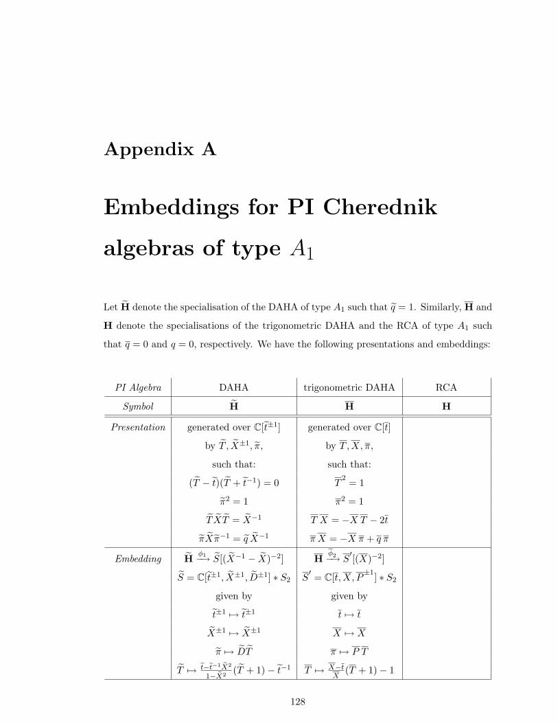
Appendix A
Embeddings for PI Cherednik
algebras of type A1
Let H denote the specialisation of the DAHA of type A1 such that q = 1. Similarly, H and
H denote the specialisations of the trigonometric DAHA and the RCA of type A1 such
that q = 0 and q = 0, respectively. We have the following presentations and embeddings:
PI Algebra DAHA trigonometric DAHA RCA
Symbol H H H
Presentation generated over C[t±1] generated over C[t]
by T , X±1, π, by T ,X, π,
such that: such that:
(T − t)(T + t−1) = 0 T2 = 1
π2 = 1 π2 = 1
T XT = X−1 T X = −X T − 2t
πXπ−1 = q X−1 πX = −X π + q π
Embedding Hφ1−→ S[(X−1 − X)−2] H
φ2−→ S′[(X)−2]
S = C[t±1, X±1, D±1] ∗ S2 S′ = C[t,X, P±1] ∗ S2
given by given by
t±1 7→ t±1 t 7→ t
X±1 7→ X±1 X 7→ X
π 7→ DT π 7→ P T
T 7→ t−t−1X2
1−X2(T + 1)− t−1 T 7→ X−t
X(T + 1)− 1
128
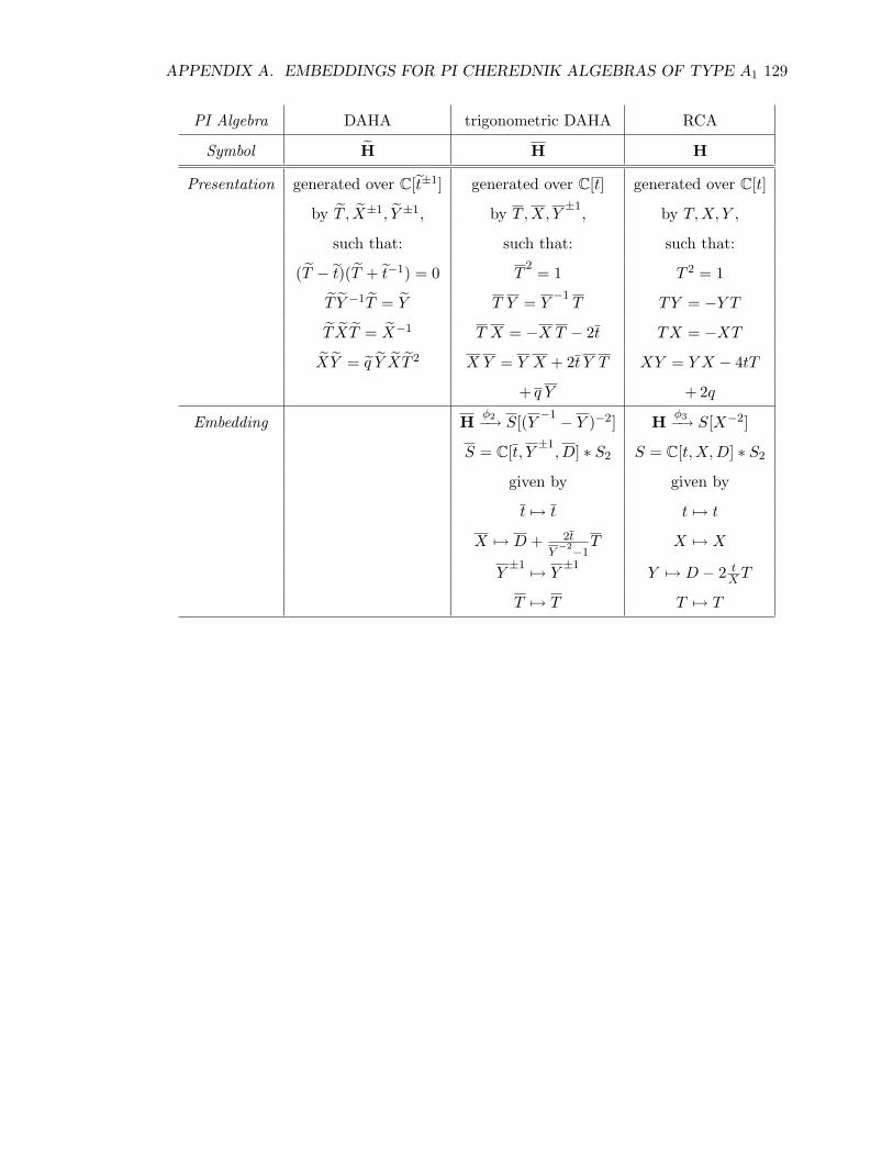
APPENDIX A. EMBEDDINGS FOR PI CHEREDNIK ALGEBRAS OF TYPE A1 129
PI Algebra DAHA trigonometric DAHA RCA
Symbol H H H
Presentation generated over C[t±1] generated over C[t] generated over C[t]
by T , X±1, Y ±1, by T ,X, Y ±1, by T,X, Y ,
such that: such that: such that:
(T − t)(T + t−1) = 0 T2 = 1 T 2 = 1
T Y −1T = Y T Y = Y−1T TY = −Y T
T XT = X−1 T X = −X T − 2t TX = −XT
XY = q Y XT 2 X Y = Y X + 2t Y T XY = Y X − 4tT
+ q Y +2q
Embedding Hφ2−→ S[(Y −1 − Y )−2] H
φ3−→ S[X−2]
S = C[t, Y ±1, D] ∗ S2 S = C[t,X,D] ∗ S2
given by given by
t 7→ t t 7→ t
X 7→ D + 2t
Y−2−1
T X 7→ X
Y±1 7→ Y
±1Y 7→ D − 2 t
XT
T 7→ T T 7→ T
References
[BBG97] J. Bernstein, A. Braverman, and D. Gaitsgory. The Cohen-Macaulay property
of the category of (g, k)-modules. Selecta Math. (N.S.), 3(3):303–314, 1997.
[BEG03] Y. Berest, P. Etingof, and V. Ginzburg. Finite-dimensional representations of
rational Cherednik algebras. Int. Math. Res. Not., (19):1053–1088, 2003.
[Ben93] D. J. Benson. Polynomial invariants of finite groups, volume 190 of London
Mathematical Society Lecture Note Series. Cambridge University Press, Cam-
bridge, 1993.
[BG96] A. Braverman and D. Gaitsgory. Poincare-Birkhoff-Witt theorem for quadratic
algebras of Koszul type. J. Algebra, 181(2):315–328, 1996.
[BG02] K. A. Brown and K. R. Goodearl. Lectures on algebraic quantum groups. Ad-
vanced Courses in Mathematics. CRM Barcelona. Birkhauser Verlag, Basel,
2002.
[BG03] K. A. Brown and I. Gordon. Poisson orders, symplectic reflection algebras and
representation theory. J. Reine Angew. Math., 559:193–216, 2003.
[BGS96] A. Beilinson, V. Ginzburg, and W. Soergel. Koszul duality patterns in represen-
tation theory. J. Amer. Math. Soc., 9(2):473–527, 1996.
[BR75] W. Borho and R. Rentschler. Oresche Teilmengen in Einhullenden Algebren.
Math. Ann., 217(3):201–210, 1975.
[Bro02] K. A. Brown. Symplectic reflection algebras. In Proceedings of the All Ireland
Algebra Days, 2001 (Belfast), number 50, pages 27–49, 2002.
[Che95] I. Cherednik. Double affine Hecke algebras and Macdonald’s conjectures. Ann.
of Math. (2), 141(1):191–216, 1995.
130
REFERENCES 131
[Che03] I. Cherednik. Double affine Hecke algebras and difference Fourier transforms.
Invent. Math., 152(2):213–303, 2003.
[Che04] I. Cherednik. Diagonal coinvariants and double affine Hecke algebras. Int. Math.
Res. Not., (16):769–791, 2004.
[Che05] I. Cherednik. Double affine Hecke algebras, volume 319 of London Mathematical
Society Lecture Note Series. Cambridge University Press, Cambridge, 2005.
[CO03] I. Cherednik and V. Ostrik. From double Hecke algebra to Fourier transform.
Selecta Math. (N.S.), 9(2):161–249, 2003.
[CR87a] C. W. Curtis and I. Reiner. Methods of representation theory. Vol. I. Pure and
Applied Mathematics (New York). John Wiley & Sons Inc., New York, 1987.
With applications to finite groups and orders, A Wiley-Interscience Publication.
[CR87b] C. W. Curtis and I. Reiner. Methods of representation theory. Vol. II. Pure and
Applied Mathematics (New York). John Wiley & Sons Inc., New York, 1987.
With applications to finite groups and orders, A Wiley-Interscience Publication.
[Dre04] J.-M. Drezet. Luna’s slice theorem and applications.
http://www.hindawi.co.uk/books/ 9775945127/B977594512700003X.pdf, 2004.
[Dri86] V. G. Drinfeld. Degenerate affine Hecke algebras and Yangians. Funct. Anal.
Appl., 20:62–64, 1986.
[Dun89] C. F. Dunkl. Differential-difference operators associated to reflection groups.
Trans. Amer. Math. Soc., 311(1):167–183, 1989.
[EG02] P. Etingof and V. Ginzburg. Symplectic reflection algebras, Calogero-
Moser space, and deformed Harish-Chandra homomorphism. Invent. Math.,
147(2):243–348, 2002.
[Eis95] D. Eisenbud. Commutative algebra, volume 150 of Graduate Texts in Mathemat-
ics. Springer-Verlag, New York, 1995. With a view toward algebraic geometry.
[FSR05] W. Ferrer Santos and A. Rittatore. Actions and invariants of algebraic groups,
volume 269 of Pure and Applied Mathematics (Boca Raton). Chapman &
Hall/CRC, Boca Raton, FL, 2005.
REFERENCES 132
[Gor03a] I. Gordon. Baby Verma modules for rational Cherednik algebras. Bull. London
Math. Soc., 35(3):321–336, 2003.
[Gor03b] I. Gordon. On the quotient ring by diagonal invariants. Invent. Math.,
153(3):503–518, 2003.
[Gor05] I. Gordon. Representation theory of symplectic reflection algebras. Unpublished
notes for postgarduate lecture course, 2005.
[GP00] M. Geck and G. Pfeiffer. Characters of finite Coxeter groups and Iwahori-Hecke
algebras, volume 21 of London Mathematical Society Monographs. New Series.
The Clarendon Press Oxford University Press, New York, 2000.
[GS04] I. Gordon and S. P. Smith. Representations of symplectic reflection algebras
and resolutions of deformations of symplectic quotient singularities. Math. Ann.,
330(1):185–200, 2004.
[GS05] I. Gordon and J. T. Stafford. Rational Cherednik algebras and Hilbert schemes.
Adv. Math., 198(1):222–274, 2005.
[GS06] I. Gordon and J. T. Stafford. Rational Cherednik algebras and Hilbert schemes
ii: Representations and sheaves. Duke Math. J., 132(1):73–135, 2006.
[GU89] A. Gyoja and K. Uno. On the semisimplicity of Hecke algebras. J. Math. Soc.
Japan, 41(1):75–79, 1989.
[GW89] K. R. Goodearl and R. B. Warfield, Jr. An introduction to noncommutative
Noetherian rings, volume 16 of London Mathematical Society Student Texts.
Cambridge University Press, Cambridge, 1989.
[Gyo95] A. Gyoja. Modular representation theory over a ring of higher dimension with
applications to Hecke algebras. J. Algebra, 174(2):553–572, 1995.
[Hai94] M. D. Haiman. Conjectures on the quotient ring by diagonal invariants. J.
Algebraic Combin., 3(1):17–76, 1994.
[Har77] R. Hartshorne. Algebraic geometry. Springer-Verlag, New York, 1977. Graduate
Texts in Mathematics, No. 52.
REFERENCES 133
[Hec91] G. J. Heckman. A remark on the Dunkl differential-difference operators. In
Harmonic analysis on reductive groups (Brunswick, ME, 1989), volume 101 of
Progr. Math., pages 181–191. Birkhauser Boston, 1991.
[Hum90] J. E. Humphreys. Reflection groups and Coxeter groups, volume 29 of Cambridge
Studies in Advanced Mathematics. Cambridge University Press, Cambridge, 2nd
edition, 1990.
[Kan01] R. Kane. Reflection groups and invariant theory. CMS Books in Mathemat-
ics/Ouvrages de Mathematiques de la SMC, 5. Springer-Verlag, New York, 2001.
[Kir97] A. A. Kirillov, Jr. Lectures on affine Hecke algebras and Macdonald’s conjectures.
Bull. Amer. Math. Soc. (N.S.), 34(3):251–292, 1997.
[Kun85] E. Kunz. Introduction to commutative algebra and algebraic geometry.
Birkhauser Boston Inc., Boston, MA, 1985. Translated from the German by
Michael Ackerman, With a preface by David Mumford.
[Lor96] M. Lorenz. Regularity of multiplicative invariants. Comm. Algebra, 24(3):1051–
1055, 1996.
[Lus89] G. Lusztig. Affine Hecke algebras and their graded version. J. Amer. Math.
Soc., 2(3):599–635, 1989.
[Mac03] I. G. Macdonald. Affine Hecke algebras and orthogonal polynomials, volume 157
of Cambridge Tracts in Mathematics. Cambridge University Press, Cambridge,
2003.
[Mar95] R. Martin. Skew group rings and maximal orders. Glasgow Math. J., 37(2):249–
263, 1995.
[Mat86] H. Matsumura. Commutative ring theory, volume 8 of Cambridge Studies in Ad-
vanced Mathematics. Cambridge University Press, Cambridge, 1986. Translated
from the Japanese by M. Reid.
[Mil98] J. S. Milne. Lectures on etale cohomology.
www.jmilne.org/math/CourseNotes/math732.pdf, 1998.
REFERENCES 134
[MR87] J. C. McConnell and J. C. Robson. Noncommutative Noetherian rings. Pure and
Applied Mathematics (New York). John Wiley & Sons Ltd., Chichester, 1987.
With the cooperation of L. W. Small, A Wiley-Interscience Publication.
[New78] P. E. Newstead. Introduction to moduli problems and orbit spaces, volume 51 of
Tata Institute of Fundamental Research Lectures on Mathematics and Physics.
Tata Institute of Fundamental Research, Bombay, 1978.
[Obl04] A. Oblomkov. Double affine Hecke algebras and Calogero-Moser spaces. Repre-
sent. Theory, 8:243–266 (electronic), 2004.
[Opd98] E. M. Opdam. Lectures on Dunkl operators. preprint math.RT/9812007, 1998.
[Pas77] D. S. Passman. The algebraic structure of group rings. Wiley-Interscience [John
Wiley & Sons], New York, 1977. Pure and Applied Mathematics.
[Pas89] D. S. Passman. Infinite crossed products, volume 135 of Pure and Applied Math-
ematics. Academic Press Inc., Boston, MA, 1989.
[Rot79] J. J. Rotman. An introduction to homological algebra, volume 85 of Pure and Ap-
plied Mathematics. Academic Press Inc. [Harcourt Brace Jovanovich Publishers],
New York, 1979.
[Rou05] R. Rouquier. Representations of rational Cherednik algebras. preprint
math.RT/0504600, 2005.
[Row88] L. H. Rowen. Ring theory. Vol. I, volume 127 of Pure and Applied Mathematics.
Academic Press Inc., Boston, MA, 1988.
[RS03] A. Ram and A. V. Shepler. Classification of graded Hecke algebras for complex
reflection groups. Comment. Math. Helv., 78(2):308–334, 2003.
[VV04] M. Varagnolo and E. Vasserot. From double affine Hecke algebras to quantized
affine Schur algebras. Int. Math. Res. Not., (26):1299–1333, 2004.
[Wit05] S. Witherspoon. Twisted graded hecke algebras. preprint math.RT/0506152,
2005.


![FORMAL HECKE ALGEBRAS AND ALGEBRAIC ORIENTED … · arXiv:1208.4114v4 [math.RA] 27 Mar 2014 FORMAL HECKE ALGEBRAS AND ALGEBRAIC ORIENTED COHOMOLOGY THEORIES ALEX HOFFNUNG, JOSE MALAG´](https://img.pdfslide.net/doc/110x75/5f49e94c4ae1e674ed145844/formal-hecke-algebras-and-algebraic-oriented-arxiv12084114v4-mathra-27-mar.jpg)
![CHEREDNIK ALGEBRAS AND CALOGERO-MOSER … · arxiv:1708.09764v2 [math.rt] 7 sep 2017 cÉdric bonnafÉ raphaËl rouquier cherednik algebras and calogero-moser cells](https://img.pdfslide.net/doc/110x75/5afa3f047f8b9a5f588f3309/cherednik-algebras-and-calogero-moser-170809764v2-mathrt-7-sep-2017-cdric.jpg)

![Automorphisms of Generic Iwahori-Hecke Algebras and Integral … · 2017-02-05 · Automorphisms of Generic Iwahori]Hecke Algebras and Integral Group Rings of Finite Coxeter Groups*](https://img.pdfslide.net/doc/110x75/5f6ff7728095716e045b5abf/automorphisms-of-generic-iwahori-hecke-algebras-and-integral-2017-02-05-automorphisms.jpg)