Embed Size (px)
Citation preview
“BinHan˙mmnp” — 2013/1/13 — 11:15 — page 18 — #1i
i
i
i
i
i
i
i
Math. Model. Nat. Phenom.
Vol. 8, No. 1, 2013, pp. 18–47
DOI: 10.1051/mmnp/20138102
Properties of Discrete Framelet Transforms
B. Han∗
Department of Mathematical and Statistical Sciences, University of AlbertaEdmonton, Alberta T6G 2G1, Canada
Abstract. As one of the major directions in applied and computational harmonic analysis, theclassical theory of wavelets and framelets has been extensively investigated in the function set-ting, in particular, in the function space L2(R
d). A discrete wavelet transform is often regardedas a byproduct in wavelet analysis by decomposing and reconstructing functions in L2(R
d) vianested subspaces of L2(R
d) in a multiresolution analysis. However, since the input/output dataand all filters in a discrete wavelet transform are of discrete nature, to understand better theperformance of wavelets and framelets in applications, it is more natural and fundamental to di-rectly study a discrete framelet/wavelet transform and its key properties. The main topic of thispaper is to study various properties of a discrete framelet transform purely in the discrete/digitalsetting without involving the function space L2(R
d). We shall develop a comprehensive theoryof discrete framelets and wavelets using an algorithmic approach by directly studying a discreteframelet transform. The connections between our algorithmic approach and the classical theoryof wavelets and framelets in the function setting will be addressed. Using tensor product ofunivariate complex-valued tight framelets, we shall also present an example of directional tightframelets in this paper.
Keywords and phrases: discrete framelet transform, perfect reconstruction, sparsity, stabil-ity, dual framelet filter banks, discrete affine systems, linear-phase moments, vanishing moments,sum rules
Mathematics Subject Classification: 42C40, 42C15
1. Introduction and Motivations
In this paper we study a discrete framelet/wavelet transform and its various properties. To explainour motivations and to provide necessary background, let us first briefly outline the classical theory ofwavelets and framelets in the function space L2(R
d).Let M be a d × d invertible real-valued matrix. For any square integrable function f ∈ L2(R
d),throughout the paper we shall adopt the following notation:
fM;k,n(x) := [[M; k, n]]f(x) := | det(M)|1/2e−in·Mxf(Mx− k), x, k, n ∈ Rd, (1.1)
where i denotes the imaginary unit. In particular, we define fM;k := fM;k,0. Let Ψ be a (finite) subset ofL2(R
d). The following homogeneous M-affine (or M-wavelet) system
∗Corresponding author. E-mail: [email protected]
c© EDP Sciences, 2013
Article published by EDP Sciences and available at http://www.mmnp-journal.org or http://dx.doi.org/10.1051/mmnp/20138102
“BinHan˙mmnp” — 2013/1/13 — 11:15 — page 19 — #2i
i
i
i
i
i
i
i
B. Han Properties of Discrete Framelet Transforms
AS(Ψ) := ψMj ;k : j ∈ Z, k ∈ Zd, ψ ∈ Ψ, (1.2)
has been extensively studied in the function space L2(Rd) in the literature of wavelet analysis, often
with M being an expansive integer matrix. Here we say that M is expansive if all its eigenvalues havemodulus greater than one. Elements in Ψ are often called wavelet (generating) functions. To emphasizethe dilation matrix M in an affine system, we also use ASM(Ψ) instead of AS(Ψ).
There are several different types of wavelets and framelets. The affine system AS(Ψ) could be anorthonormal basis, a tight frame, or a Riesz basis for the function space L2(R
d). For example, we saythat AS(Ψ) is a tight frame for L2(R
d) if
‖f‖2L2(Rd) =∑
j∈Z
∑
k∈Zd
∑
ψ∈Ψ|〈f, ψMj ;k〉|
2, ∀ f ∈ L2(Rd). (1.3)
It follows from (1.3) that every function f ∈ L2(Rd) has the following wavelet representation:
f =∑
j∈Z
∑
k∈Zd
∑
ψ∈Ψ〈f, ψMj ;k〉ψMj ;k (1.4)
with the series converging in L2(Rd).
One of the major tasks in wavelet analysis is to construct Ψ having some desirable properties sothat AS(Ψ) is an orthonormal basis, a tight frame, or a Riesz basis for L2(R
d). For this purpose, thedominating approach in the current literature is to use a multiresolution analysis (MRA). A sequenceVjj∈Z of closed subspaces of L2(R
d) is called a multiresolution analysis of L2(Rd) (see [2, 8, 35]) if
(i) Vj ⊆ Vj+1 and Vj = f(Mj ·) : f ∈ V0 for all j ∈ Z;(ii) ∪j∈ZVj is dense in L2(R
d) and ∩j∈ZVj = 0;(iii) There exists Φ ⊆ L2(R
d) such that the linear span of φ(· − k), k ∈ Zd, φ ∈ Φ is dense in V0.
φ(· − k) : k ∈ Zd, φ ∈ Φ is often required to be a Riesz basis or an orthonormal basis of V0. By (i), we
have Φ ⊆ V1 and therefore, Φ must be M-refinable satisfying φ(MTξ) = a(ξ)φ(ξ) for almost every ξ ∈ Rd,where φ is obtained by listing all the elements in Φ as a column vector and a is a (#Φ) × (#Φ) matrixof 2πZd-periodic Lebesgue measurable functions. Now a set Ψ of wavelet generating functions is oftenderived from φ via the following relation:
ψ(MTξ) = bψ(ξ)φ(ξ), a.e. ξ ∈ Rd, ψ ∈ Ψ, (1.5)
where bψ is some 1×(#Φ) row vector of 2πZd-periodic measurable functions. By appropriately construct-
ing a and bψ, ψ ∈ Ψ , one obtains an affine system AS(Ψ) so that it is an orthonormal basis, a tight frame,or a Riesz basis for L2(R
d). There are a vast literature on this topic, to mention a very tiny portion ofthem, see [2, 8, 35,36,39,40] and numerous references therein.
We now discuss the associated discrete wavelet/framelet transform in the function setting by decompos-ing and reconstructing functions in L2(R
d) via nested subspaces of L2(Rd) in a multiresolution analysis.
For simplicity of discussion, we assume that Φ = φ is a singleton and AS(Ψ) is a tight frame for L2(Rd)
with Ψ being derived from an M-refinable function φ via (1.5). To compute the wavelet coefficients〈f, ψMj ;k〉 in the wavelet representation of f in (1.4), a widely accepted approach in the literature consistsof two parts: projection (or discretization) and a discrete transform. To discretize a function f fromthe continuum domain into the discrete/digital domain, one selects a large enough integer J so that thefunction f is well approximated by the projected function PJf :=
∑k∈Zd(DJf)(k)φMJ ;k, where Dj , j ∈ Z
are the discretization (or approximation) operators defined by
Dj : L2(Rd) → l2(Z
d) with Djf := 〈f, φMj ;k〉k∈Zd . (1.6)
19
“BinHan˙mmnp” — 2013/1/13 — 11:15 — page 20 — #3i
i
i
i
i
i
i
i
B. Han Properties of Discrete Framelet Transforms
Therefore, most information of the function f is encoded now in the discrete sequence DJf . Next adiscrete transform is employed to compute all wavelet coefficients 〈f, ψMj ;k〉, j < J and k ∈ Zd using only
the discrete sequence DJf and the Fourier coefficients of a and bψ, ψ ∈ Ψ . More precisely, rewrite the
relations φ(MTξ) = a(ξ)φ(ξ) and ψ(MTξ) = b(ξ)φ(ξ) as
φ(x) = dM∑
k∈Zd
a(k)φ(Mx− k) and ψ(x) = dM∑
k∈Zd
b(k)φ(Mx− k),
where dM := | det(M)| and∑
k∈Zd a(k)e−ik·ξ := a(ξ), that is, a(k)k∈Zd is the sequence of the Fouriercoefficients of a. Then one can easily deduce that
(Dj−1f)(n) = d1/2M
∑
k∈Zd
a(k−Mn)(Djf)(k), 〈f, ψMj−1;n〉 = d1/2M
∑
k∈Zd
b(k−Mn)(Djf)(k).
Now one can easily see that all the coefficients 〈f, ψMj ;n〉, j < J and n ∈ Zd can be computed recursively
using DJf and the Fourier coefficients of a and bψ, ψ ∈ Ψ . This discrete transform is called a fast wavelettransform in the literature (see Sections 2 and 4 for more detail).
However, the mapping DJ in (1.6) may fail to be onto and therefore, not all signals in l2(Zd) can be
exactly reconstructed by the associated discrete wavelet transform. This is not desirable in both theoryand application, since 〈f, φMJ ;k〉 is often numerically computed by quadrature formulas and therefore, thenumerically computed sequence DJf may no longer fall inside the range of DJ . Even if the mapping in(1.6) is onto, it is highly nontrivial to practically implement the discretization in (1.6) using a refinablefunction φ. On the contrary, a practical sampling device for discretizating a function in the continuumdomain is often pre-designed. For example, a digital camera can be used to convert a natural scenefrom the continuum domain into the digital world. It is more realistic to assume that a digital deviceemploying (1.6) uses a pre-designed function φ = η and a particularly selected integer J . Therefore,a discretization or a measurement of f is given in advance by 〈f, ηMJ ;k〉k∈Zd , instead of the one in(1.6) using a refinable function φ. These difficulties motivate us to directly study a discrete framelettransform without associating it to an underlying affine system in the function space L2(R
d). To ourbest knowledge, almost all papers and books on wavelet analysis deal with wavelets in the function spaceL2(R
d) and a discrete framelet transform is always regarded as a consequence of a multiresolution analysisas outlined above. Though it is very natural and fundamental to directly study a discrete framelet/wavelettransform, this algorithmic approach has barely been adopted before in wavelet analysis and harmonicanalysis, including books oriented for engineers such as [39,40].
The structure of the paper is as follows. In Section 2, we shall recall the one-level discrete framelettransform and then study its perfect reconstruction property. We shall explain the differences between adiscrete framelet transform and its special case–a discrete wavelet transform. In Section 3, we study sev-eral basic key properties that are closely related to sparsity of a discrete framelet transform in the discretesetting, in particular, properties such as vanishing moments, sum rules, and polynomial reproduction. InSection 4, we shall introduce the notion of stability of a discrete framelet transform and discrete affinesystems. Then we shall study the stability issue of a discrete framelet transform, which is one of themost important and challenging aspects of wavelet analysis. In Section 5 we shall investigate symmetryproperty of wavelets/framelets and the important role played by linear-phase moments in wavelet analy-sis. In Section 6, we shall study connections between dual framelet filter banks and frequency-based dualframelets. We show that every dual framelet filter bank naturally corresponds to a frequency-based dualframelet without any a priori condition. Finally, in Section 7 we present an example of directional tightframelets using tensor product of univariate complex-valued tight framelets.
20
“BinHan˙mmnp” — 2013/1/13 — 11:15 — page 21 — #4i
i
i
i
i
i
i
i
B. Han Properties of Discrete Framelet Transforms
2. Perfect Reconstruction of Discrete Framelet Transforms
In this section, we recall one-level discrete framelet transforms (DFrT) in dimension d. Among the threefundamental properties of a discrete framelet transform: prefect reconstruction, sparsity, and stability,we address in this section the most basic property—the perfect reconstruction property.
To introduce a discrete framelet transform, we need some definitions and concepts first. By l(Zd)we denote the linear space of all sequences v : Zd → C of complex numbers on Zd. For v ∈ l(Zd), weoften write v = v(k)k∈Zd . Theoretically, a discrete input data is often regarded as an element in l(Zd).Similarly, by l0(Z
d) we denote the linear space of all sequences u = u(k)k∈Zd : Zd → C on Zd such thatk ∈ Zd : u(k) 6= 0 is a finite set. An element in l0(Z
d) is often regarded as a finite-impulse-response(FIR) filter or a finitely supported mask. In this paper, we use u for a general filter and v for a generaldata.
A discrete framelet transform can be described using two linear operators—the subdivision operatorand the transition operator. More precisely, for a filter u ∈ l0(Z
d) and a d × d integer matrix M, thesubdivision operator Su,M : l(Zd) → l(Zd) and the transition operator Tu,M : l(Zd) → l(Zd) are defined tobe
[Su,Mv](n) := | det(M)|∑
k∈Zd
v(k)u(n−Mk), n ∈ Zd, (2.1)
[Tu,Mv](n) := | det(M)|∑
k∈Zd
v(k)u(k−Mn), n ∈ Zd (2.2)
for v ∈ l(Zd). The transition operator is used for decomposition and plays the role of coarsening andfrequency-separating the data to lower resolution levels; while the subdivision operator is used for recon-struction and plays the role of refining and predicting the data to higher resolution levels.
For a d× d invertible integer matrix M, we frequently use the following notations:
dM := | det(M)|, ΓM := (M[0, 1)d) ∩ Zd and ΩM := ((MT)−1Zd) ∩ [0, 1)d. (2.3)
In other words, ΓM = γ1, . . . , γdM denotes a complete set of representatives of the distinct cosets ofthe quotient group Zd/[MZd], while ΩM = ω1, . . . , ωdM denotes a complete set of representatives of thedistinct cosets of the quotient group [(MT)−1Zd]/Zd. Note that ΩM = (MT)−1ΓMT .
It is often convenient to use the formal Fourier series (or symbol) v of a sequence v = v(k)k∈Zd , whichis defined to be v(ξ) :=
∑k∈Zd v(k)e−ik·ξ for ξ ∈ Rd, where k · ξ := k1ξ1 + · · ·+ kdξd for k = (k1, . . . , kd)
T
and ξ = (ξ1, . . . , ξd)T. Note that v = v(k)k∈Zd is simply the sequence of Fourier coefficients of v. Quite
often, one only needs to deal with v in the space l2(Zd), equipped with the inner product:
〈v, w〉 :=∑
k∈Zd
v(k)w(k), v, w ∈ l2(Zd) (2.4)
and ‖v‖2l2(Zd) := 〈v, v〉 <∞. In terms of Fourier series, we have
Su,Mv(ξ) = dMv(MTξ)u(ξ), Tu,Mv(ξ) =
∑
ω∈ΩM
v((MT)−1ξ + 2πω)u((MT)−1ξ + 2πω). (2.5)
We now describe a one-level standard (multidimensional) discrete framelet transform which consists oftwo parts: a one-level framelet decomposition and a one-level framelet reconstruction. Let u0, . . . , us ∈l0(Z
d) be filters for decomposition. For a given data v ∈ l(Zd), a one-level framelet decompositionemploying the filter bank u0, . . . , us is
wℓ := d−1/2M Tuℓ,Mv, ℓ = 0, . . . , s, (2.6)
21

“BinHan˙mmnp” — 2013/1/13 — 11:15 — page 22 — #5i
i
i
i
i
i
i
i
B. Han Properties of Discrete Framelet Transforms
where wℓ are called sequences of framelet coefficients of the input signal v. We can group all sequencesof framelet coefficients together and define a framelet decomposition (or analysis) operator W : l(Zd) →(l(Zd))1×(s+1) employing the filter bank u0, . . . , us as follows:
Wv := d−1/2M (Tu0,Mv, . . . , Tus,Mv), v ∈ l(Zd). (2.7)
Let u0, . . . , us ∈ l0(Zd) be filters for reconstruction. A one-level framelet reconstruction employ-
ing the filter bank u0, . . . , us can be described by a framelet reconstruction (or synthesis) operatorV : (l(Zd))1×(s+1) → l(Zd) which is defined to be
V(w0, . . . , ws) := d−1/2M
s∑
ℓ=0
Suℓ,Mwℓ, w0, . . . , ws ∈ l(Zd). (2.8)
The role played by the factor d−1/2M in (2.7) and (2.8) is to balance or preserve energy between the
input signal and its framelet coefficients. We shall explain this issue later in this section. We denote aframelet decomposition operator employing the filter bank u0, . . . , us by W and similarly, a framelet
reconstruction operator employing the filter bank u0, . . . , us by V.One of the fundamental properties of a discrete framelet transform is the prefect reconstruction prop-
erty: VWv = v for all input data v. We say that a discrete framelet transform employing a filter bank(u0, . . . , us, u0, . . . , us), or simply, a filter bank (u0, . . . , us, u0, . . . , us) has the perfect reconstruc-
tion (PR) property if VWv = v for all input data v ∈ l(Zd). By δ we denote the Dirac (or Kronecker)sequence such that
δ(0) = 1 and δ(k) = 0, ∀ k 6= 0. (2.9)
The following is a necessary and sufficient condition for the perfect reconstruction property of a generalone-level discrete framelet transform:
Theorem 2.1. Let u0, . . . , us, u0, . . . , us ∈ l0(Zd). Then the following statements are equivalent:
(i) (u0, . . . , us, u0, . . . , us) has perfect reconstruction property, that is, for all v ∈ l(Zd),
v = VWv = d−1M
s∑
ℓ=0
Suℓ,MTuℓ,Mv, (2.10)
where W and V are defined in (2.7) and (2.8), respectively.(ii) The identity in (2.10) holds for all v ∈ l0(Z
d).(iii) The identity in (2.10) holds for dM particular sequences v = δ(· − γ), γ ∈ ΓM.(iv) The following perfect reconstruction condition holds: for all ω ∈ ΩM and ξ ∈ Rd,
u0(ξ)u0(ξ + 2πω) + u1(ξ)u1(ξ + 2πω) + · · ·+ us(ξ)us(ξ + 2πω) = δ(ω). (2.11)
Proof. (i)=⇒(ii)=⇒(iii) is trivial by l0(Zd) ⊆ l(Zd). By (2.5), we have
d−1M
[Suℓ,MTuℓ,Mv](ξ) = Tuℓ,Mv(MTξ)uℓ(ξ) =
∑
ω∈ΩM
v(ξ + 2πω) uℓ(ξ + 2πω)uℓ(ξ). (2.12)
Therefore, (2.10) holds if and only if
v(ξ) =∑
ω∈ΩM
v(ξ + 2πω)
s∑
ℓ=0
uℓ(ξ + 2πω)uℓ(ξ). (2.13)
Plugging v = δ(· − γ) into (2.13) and noting δ(· − γ)(ξ) = e−iγ·ξ, we see that (2.13) becomes
1 =∑
ω∈ΩM
eiγ·2πωs∑
ℓ=0
uℓ(ξ + 2πω)uℓ(ξ).
22
“BinHan˙mmnp” — 2013/1/13 — 11:15 — page 23 — #6i
i
i
i
i
i
i
i
B. Han Properties of Discrete Framelet Transforms
Since d−1/2M (eiγ·2πω)γ∈ΓM,ω∈ΩM
is a unitary matrix, we deduce that (2.11) must hold. Therefore,(iii)=⇒(iv). If (2.11) is satisfied, then (2.13) holds trivially for all v ∈ l0(Z
d). Hence, (iv)=⇒(ii).To complete the proof, we show that (ii)=⇒(i). Note that all filters u0, . . . , us, u0, . . . , us are supported
inside a ball Br(0) with center 0 and radius r. Let v ∈ l(Zd) and n ∈ Zd. We shall deduce from (ii) that
d−1M
s∑
ℓ=0
[Suℓ,MTuℓ,Mv](n) = v(n). (2.14)
Define Kn := M−1(n − Br(0)). Define a finitely supported sequence vn ∈ l0(Zd) by vn(k) := v(k) for
all k ∈ Zd ∩ (Br(0) + MKn), and vn(k) = 0 otherwise. Clearly, vn ∈ l0(Zd) and vn(n) = v(n) since
n ∈ Zd ∩ (Br(0) +MKn). For all k ∈ Zd ∩Kn, since all filters are supported inside Br(0),
[Tuℓ,Mv](k) = dM∑
j∈Zd
v(j)uℓ(j−Mk) = dM∑
j∈Zd∩(Br(0)+MKn)
vn(j)uℓ(j−Mk) = [Tuℓ,Mvn](k).
Therefore, we deduce that
d−1M
s∑
ℓ=0
[Suℓ,MTuℓ,Mv](n) =s∑
ℓ=0
∑
k∈Zd∩Kn
[Tuℓ,Mv](k)uℓ(n−Mk)
=
s∑
ℓ=0
∑
k∈Zd∩Kn
[Tuℓ,Mvn](k)uℓ(n−Mk) = d−1M
s∑
ℓ=0
[Suℓ,MTuℓ,Mvn](n) = vn(n) = v(n),
where we used (ii) and the fact that vn(n) = v(n). Hence, (ii)=⇒(i).
The condition in (2.11) can be equivalently rewritten as the following matrix form:
u0(ξ + 2πω1) · · · us(ξ + 2πω1)
.... . .
...u0(ξ + 2πωdM) · · · us(ξ + 2πωdM)
u0(ξ + 2πω1) · · · us(ξ + 2πω1)
.... . .
...u0(ξ + 2πωdM) · · · us(ξ + 2πωdM)
⋆
= IdM , (2.15)
where ω1, . . . , ωdM := ΩM. A filter bank satisfying the perfect reconstruction condition in (2.15) iscalled a dual M-framelet filter bank. It follows trivially from the perfect reconstruction condition in (2.15)that (u0, . . . , us, u0, . . . , us) is a dual M-framelet filter bank if and only if (u0, . . . , us, u0, . . . , us)
is a dual M-framelet filter bank. In other words, VW = Id l(Z) if and only if VW = Id l(Z). In particular,a dual M-framelet filter bank with s = dM − 1 is called a biorthogonal M-wavelet filter bank which, by thefollowing result, is a nonredundant filter bank.
Proposition 2.2. Let (u0, . . . , us, u0, . . . , us) be a dual M-framelet filter bank. Let the framelet
decomposition operator W : l(Zd) → (l(Zd))1×(s+1) and framelet reconstruction operator V :(l(Zd))1×(s+1) → l(Zd) be defined in (2.7) and (2.8). Then the following statements are equivalent:
(i) W is onto, or V is one-to-one.
(ii) VW = Id l(Zd) and WV = Id(l(Zd))1×(s+1) , that is, V−1 = W and W−1 = V.(iii) s = dM − 1, where dM := | det(M)|.
The same conclusion holds if l(Zd) is replaced by l2(Zd) or l0(Z
d).
Proof. (ii)=⇒(i) is trivial. Note that VW = Id l(Zd) follows directly from the perfect reconstruction
property. Using WVWw = Ww, if W is onto, then W(l(Zd))1×(s+1) = l(Zd) and we must have WV =
Id(l(Zd))1×(s+1) . By VW = Id l(Zd), we have VWV = V and therefore, V(WV − Id(l(Zd))1×(s+1)) = 0. If V is
one-to-one, we must have WV = Id(l(Zd))1×(s+1) . Hence, (i)=⇒(ii).
23
“BinHan˙mmnp” — 2013/1/13 — 11:15 — page 24 — #7i
i
i
i
i
i
i
i
B. Han Properties of Discrete Framelet Transforms
Now we prove (ii) ⇐⇒ (iii). Suppose that (ii) holds. Then WV = Id(l(Zd))1×(s+1) implies
d−1M Tuℓ,M
(Su0,Mw0 + · · ·+ Sus,Mws
)= wℓ, ∀ w0, . . . , ws ∈ l(Zd), ℓ = 0, . . . , s. (2.16)
Taking the Fourier series on both sides of (2.16), we see that (2.16) is equivalent to
w0(ξ)∑
ω∈ΩM
u0((MT)−1ξ + 2πω) uℓ((MT)−1ξ + 2πω) + · · ·
+ ws(ξ)∑
ω∈ΩM
us((MT)−1ξ + 2πω) uℓ((MT)−1ξ + 2πω) = wℓ(ξ)
for all ℓ = 0, . . . , s. It is trivial to see that the above identities hold if and only if
∑
ω∈ΩM
um((MT)−1ξ + 2πω) uℓ((MT)−1ξ + 2πω) = δ(ℓ−m), ℓ,m = 0, . . . , s.
Rewriting the above identities into matrix form, we see that WV = Id(l(Zd))1×(s+1) if and only if
u0(ξ + 2πω1) · · · us(ξ + 2πω1)
.... . .
...u0(ξ + 2πωdM) · · · us(ξ + 2πωdM)
⋆ u0(ξ + 2πω1) · · · us(ξ + 2πω1)
.... . .
...u0(ξ + 2πωdM) · · · us(ξ + 2πωdM)
= Is+1. (2.17)
Combining (2.17) with (2.15), we conclude that we must have s+ 1 = dM. Therefore, (ii)=⇒(iii).
Conversely, if s = dM − 1, as a square matrix, (2.15) directly implies (2.17). By the above argument,
we must have WV = Id(l(Zd))1×(s+1) . Therefore, (iii) must hold.
If l(Zd) is replaced by S := l2(Zd) or l0(Z
d), one can check that W : S → (S)1×(s+1) and V :(S)1×(s+1) → S are well defined. The same proof can be used to verify the claims.
Consequently, under a biorthogonal wavelet filter bank, any input signal v ∈ l2(Zd) has a nonredundant
representation v = Vw with the unique choice w = Wv; while under a dual framelet filter bank withs > dM, an input signal v can be represented as v = Vw from infinitely many w ∈ (l(Zd))1×(s+1) offramelet coefficients.
In the following, we explain the role played by the factor d−1/2M in (2.7) and (2.8). To do so, we need
the following simple relation, which is well known in the literature (e.g., see [5]), between the subdivisionoperator Su,M and the transition operator Tu,M acting on the space l2(Z
d).
Lemma 2.3. Let u ∈ l0(Zd) be a finitely supported filter on Zd. Then Su,M : l2(Z
d) → l2(Zd) is the
adjoint operator of Tu,M : l2(Zd) → l2(Z
d); that is, T ⋆u,M = Su,M satisfying
〈Su,Mv, w〉 = 〈T ⋆u,Mv, w〉 := 〈v, Tu,Mw〉, ∀ v, w ∈ l2(Z
d). (2.18)
Proof. By (2.5), we have Su,Mv(ξ) = dMv(MTξ)u(ξ) and hence
〈Su,Mv, w〉 =dM
(2π)d
∫
[−π,π)dv(MTξ)u(ξ)w(ξ)dξ
=1
(2π)d
∫
MT[−π,π)dv(ξ)u((MT)−1ξ)w((MT)−1ξ)dξ =
1
(2π)d
∫
[−π,π)dv(ξ)Tu,Mw(ξ)dξ,
where we used (2.5) in the last identity. Hence, (2.18) holds.
24
“BinHan˙mmnp” — 2013/1/13 — 11:15 — page 25 — #8i
i
i
i
i
i
i
i
B. Han Properties of Discrete Framelet Transforms
Note that the space (l2(Zd))1×(s+1) is equipped with the following inner product:
〈(w0, . . . , ws), (w0, . . . , ws)〉 := 〈w0, w0〉+ · · ·+ 〈ws, ws〉, w0, . . . , ws, w0, . . . , ws ∈ l2(Zd)
and ‖(w0, . . . , ws)‖2(l2(Zd))1×(s+1) := ‖w0‖
2l2(Zd) + · · ·+ ‖ws‖
2l2(Zd). Recall that
W : l2(Zd) → (l2(Z
d))1×(s+1) with Wv := d−1/2M (Tu0,Mv, . . . , Tus,Mv), v ∈ l2(Z
d) (2.19)
and
V : (l2(Zd))1×(s+1) → l2(Z
d) with V(w0, . . . , ws) := d−1/2M
s∑
ℓ=0
Suℓ,Mwℓ, (2.20)
for w0, . . . , ws ∈ l2(Zd). The adjoint operators of W and V are defined to be
W⋆ : (l2(Zd))1×(s+1) → l2(Z
d) through 〈v,W⋆w〉 := 〈Wv, w〉 (2.21)
andV⋆ : l2(Z
d) → (l2(Zd))1×(s+1) through 〈V⋆v, w〉 := 〈v,Vw〉 (2.22)
for all v ∈ l2(Zd) and w ∈ (l2(Z
d))1×(s+1). By Lemma 2.3, we have W⋆ = V and V⋆ = W.
The role played by the factor d−1/2M in (2.7) and (2.8) is explained by the following result:
Theorem 2.4. Let u0, . . . , us ∈ l0(Zd) be finitely supported sequences on Zd. Let W : l2(Z
d) →(l2(Z
d))1×(s+1) be defined in (2.19). Then the following statements are equivalent:
(i) ‖Wv‖2(l2(Zd))1×(s+1) = ‖v‖2l2(Zd) for all v ∈ l2(Z
d), that is,
‖Tu0,Mv‖2l2(Zd) + · · ·+ ‖Tus,Mv‖
2l2(Zd) = dM‖v‖
2l2(Zd), ∀ v ∈ l2(Z
d). (2.23)
(ii) 〈Wv,W v〉 = 〈v, v〉 for all v, v ∈ l2(Zd).
(iii) W⋆W = Id l2(Zd), that is, W⋆Wv = v for all v ∈ l2(Z
d).(iv) (u0, . . . , us, u0, . . . , us) is a dual M-framelet filter bank.
Proof. Obviously, (ii)=⇒(i). Note that (i) implies 〈W⋆Wv, v〉 = 〈Wv,Wv〉 = 〈v, v〉. Using the well-known polarization identity, it is straightforward to see that 〈Wv,W v〉 = 〈W⋆Wv, v〉 = 〈v, v〉. Hence,(i)=⇒(ii). The equivalence between (ii) and (iii) is trivial. Note that W⋆ = V. The equivalence between(iii) and (iv) follows directly from Theorem 2.1.
A filter bank u0, . . . , us is called a tight M-framelet filter bank if (u0, . . . , us, u0, . . . , us) is adual M-framelet filter bank. In particular, a tight M-framelet filter bank with s = dM − 1 is called anorthogonal M-wavelet filter bank. By item (i) of Theorem 2.4, the energy is preserved after a tight frameletdecomposition:
∑sℓ=0 ‖wℓ‖
2l2(Zd) = ‖Wv‖2l2(Zd) = ‖v‖2l2(Zd) for all v ∈ l2(Z
d), where (w0, . . . , ws) := Wv is
the sequence of framelet coefficients. Let u0, . . . , us be an orthogonal M-wavelet filter bank. Define Was in (2.19) and V as in (2.20). By Proposition 2.2 and Theorem 2.4, we see that W = V⋆ is an invertibleorthogonal mapping satisfying 〈Wv,W v〉 = 〈v, v〉 for all v, v ∈ l2(Z
d) and V = W⋆ is an invertibleorthogonal mapping such that for all w0, . . . , ws, w0, . . . , ws ∈ l2(Z
d), 〈V(w0, . . . , ws),V(w0, . . . , ws)〉 =〈(w0, . . . , ws), (w0, . . . , ws)〉.
3. Sparsity of Discrete Framelet Transforms
One key feature of wavelets in the function space L2(Rd) is the sparse representation for smooth or
piecewise smooth functions ([2,8,35,36]). Since we deal with the discrete setting, the sparsity of a discreteframelet transform, which we shall discuss in this section, refers to the sparsity of framelet coefficients forsmooth discrete signals. We shall mention in Section 6 some connections between sparsity of a discrete
25
“BinHan˙mmnp” — 2013/1/13 — 11:15 — page 26 — #9i
i
i
i
i
i
i
i
B. Han Properties of Discrete Framelet Transforms
framelet transform and the sparse representation of a framelet/wavelet in the function space L2(Rd). In
applications, it is desirable to have as many as possible negligible framelet coefficients for smooth signals.In this section, we study several basic key mathematical properties that are closely related to sparsity ofa discrete framelet transform in the discrete setting, in particular, properties such as vanishing moments,sum rules, and polynomial reproduction. This section is mainly surveyed from the papers [24,25] as wellas [16, 19]. For the convenience of the reader, we shall provide self-contained proofs for results stated inthis section.
For an integer j = 1, . . . , d, by ∂j we denote the partial derivative with respect to the jth coordinateof Rd. Define N0 := N ∪ 0. For µ = (µ1, . . . , µd)
T ∈ Nd0 and x = (x1, . . . , xd)T ∈ Rd, we define
|µ| := |µ1| + · · · + |µd|, µ! := µ1! · · ·µd!, xµ := xµ1
1 · · ·xµd
d , and ∂µ := ∂µ1
1 · · · ∂µd
d . Moreover, we write∂ := (∂1, . . . , ∂d)
T, the gradient differentiation operator.Smooth signals are modeled by polynomials of various degrees. Let p : Rd → C be a d-variate
polynomial, that is, p(x) =∑µ∈Nd
0 ,|µ|6n pµxµ for some n ∈ N0 and if
∑|µ|=n |pµ| 6= 0, deg(p) := n is
called the (total) degree of the polynomial p. Sampling a polynomial p on the integer lattice Zd, wehave a polynomial sequence p|Zd : Zd → C which is given by [p|Zd ](k) = p(k), k ∈ Zd. If a sequencev = v(k)k∈Zd is a polynomial sequence, then a polynomial p, satisfying v(k) = p(k) for all k ∈ Zd, isuniquely determined. For simplicity of presentation, we shall use p to denote both a polynomial functionp on Rd and its induced polynomial sequence p|Zd on Zd.
For a nonnegative integer m ∈ N0, Πm denotes the space of all polynomials of (total) degree no morethan m. In particular, Π := ∪∞
m=0Πm denotes the space of all polynomials on Rd. For a polynomialp(x) =
∑µ∈Nd
0pµx
µ and a smooth function f(ξ), we use the following polynomial differentiation operatorin this section:
p(x− i∂)f(ξ) :=∑
µ∈Nd0
pµ(x− i∂)µf(ξ), (3.1)
where in case of confusion ∂ is always with respect to ξ in this paper. Using the Taylor expansion ofp(y + z) at the point y, we have p(y + z) =
∑µ∈Nd
0(∂µp)(y) z
µ
µ! . Consequently, we have
p(x− i∂)f(ξ) =∑
µ∈Nd0
(−i)|µ|
µ!∂µp(x)∂µf(ξ) =
∑
µ∈Nd0
xµ
µ![(∂µp)(−i∂)]f(ξ). (3.2)
Using Leibniz differentiation formula and (3.2), one can also verify the following generalized product rulefor differentiation:
p(x− i∂)(g(ξ)f(ξ)
)=
∑
µ∈Nd0
(−i)|µ|
µ!∂µg(ξ)[(∂µp)(x− i∂)]f(ξ). (3.3)
It follows directly from (3.2) and (3.3) that
[p(−i∂)(eix·ξf(ξ))]|ξ=0 = [p(x− i∂)f(ξ)]|ξ=0. (3.4)
For u ∈ l0(Zd) and v ∈ l(Zd), the convolution u∗v satisfying the relation u ∗ v(ξ) = u(ξ)v(ξ) is defined
to be[u ∗ v](n) :=
∑
k∈Zd
u(k)v(n− k), n ∈ Zd (3.5)
and an associated sequence v⋆ satisfying the relation v⋆(ξ) = v(ξ) by
v⋆(k) := v(−k), k ∈ Zd. (3.6)
To study basic properties of a discrete framelet transform, it is of importance to investigate how thesubdivision operator and the transition operator act on polynomial spaces. Since the subdivision andtransition operators can be expressed via the convolution operation, in the following we first study theconvolution operation acting on polynomial spaces.
26
“BinHan˙mmnp” — 2013/1/13 — 11:15 — page 27 — #10i
i
i
i
i
i
i
i
B. Han Properties of Discrete Framelet Transforms
Lemma 3.1. ([25, Proposition 2.1] and [24, (4.7)]) Let u = u(k)k∈Zd ∈ l0(Zd). Then for any d-variate
polynomial p ∈ Π, p ∗ u is a polynomial sequence with deg(p ∗ u) 6 deg(p) and
[p ∗ u](x) :=∑
k∈Zd
p(x− k)u(k) =∑
µ∈Nd0
(−i)|µ|
µ!∂µp(x)∂µu(0) = [p(x− i∂)u(ξ)]|ξ=0. (3.7)
Moreover, [∂µp] ∗ u = ∂µ[p ∗ u] for all µ ∈ Nd0 and p(· − y) ∗ u = [p ∗ u](· − y) for all y ∈ Rd.
Proof. Using the Taylor expansion, we have p(x− k) =∑µ∈Nd
0∂µp(x) (−k)µ
µ! . Hence, we deduce
[p ∗ u](x) =∑
k∈Zd
p(x− k)u(k) =∑
k∈Zd
∑
µ∈Nd0
∂µp(x)u(k)(−k)µ
µ!=
∑
µ∈Nd0
∂µp(x)∑
k∈Zd
u(k)(−k)µ
µ!.
By u(ξ) =∑
k∈Zd u(k)e−ik·ξ, we observe that ∂µu(0) = i|µ|∑
k∈Zd u(k)(−k)µ. Hence, [p ∗ u](x) =∑µ∈Nd
0
(−i)|µ|
µ! ∂µp(x)∂µu(0), from which and (3.2) we see that all the claims hold.
For an integer m ∈ N0 and smooth functions f ,g, we use the following big O notation
f(ξ) = g(ξ) +O(‖ξ − ξ0‖m), ξ → ξ0 (3.8)
to mean the following relation:
∂µf(ξ0) = ∂µg(ξ0), ∀ µ ∈ Nd0 satisfying |µ| < m. (3.9)
For a polynomial p ∈ Πm−1 of degree less than m, by (3.7), it is evident that the polynomial p ∗ udepends only on the values ∂µu(0) of u at the origin for µ ∈ Nd0 with |µ| < m. In other words, ifu, v ∈ l0(Z
d) satisfy u(ξ) = v(ξ) +O(‖ξ‖m) as ξ → 0, then p ∗ u = p ∗ v for all p ∈ Πm−1.Now we study the action of the transition operator on polynomial spaces.
Theorem 3.2. ([25, Proposition 3.1] and [24, Proposition 4.2]) Let u ∈ l0(Zd) and M be a d×d invertible
integer matrix. For any given polynomial p ∈ Π,
Tu,Mp = dM[p ∗ u⋆](M·) = p(M·) ∗ up =
∑
µ∈Nd0
dM(−i)|µ|
µ!(∂µp)(M·)∂µu(0), (3.10)
where up is any finitely supported sequence on Zd such that
up(ξ) = dMu((MT)−1ξ) +O(‖ξ‖deg(p)+1), ξ → 0. (3.11)
In particular, for any positive integer m ∈ N, the following statements are equivalent:
(1) Tu,Mp = 0 for all polynomial sequences p ∈ Πm−1.(2) Tu,Mq = 0 for all polynomial sequences q = (·)µ with µ ∈ Nd0 and |µ| = m− 1.(3) u(ξ) = O(‖ξ‖m) as ξ → 0, that is, ∂µu(0) = 0 for all µ ∈ Nd0 with |µ| < m.
Proof. Since Tu,Mp = dM[p ∗ u⋆](M·) = dM∑
k∈Zd p(M(· − M−1k))u(−k), by Lemma 3.1 and p(M(· −
M−1k)) =∑µ∈Nd
0∂µ(p(M·)) (−M−1k)µ
µ! , we see that Tu,Mp is a polynomial sequence and
dM[p ∗ u⋆](M·) =
∑
µ∈Nd0
∂µ(p(M·))dM
µ!
∑
k∈Zd
u(−k)(−M−1k)µ =∑
µ∈Nd0
(−i)|µ|
µ!∂µ(p(M·))∂µup(0),
where we used ∂µup(0) = dMi|µ| ∑
k∈Zd u(k)(M−1k)µ. Now the identities in (3.10) follow directly from(3.7). The equivalence among items (1)–(3) is a direct consequence of (3.10).
27
“BinHan˙mmnp” — 2013/1/13 — 11:15 — page 28 — #11i
i
i
i
i
i
i
i
B. Han Properties of Discrete Framelet Transforms
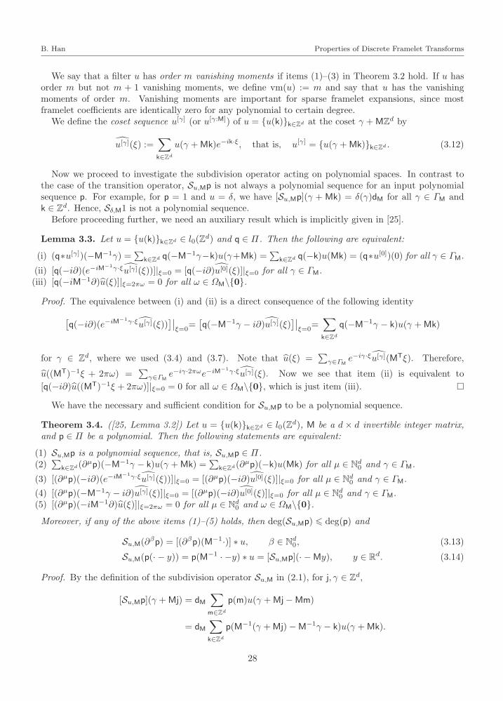
We say that a filter u has order m vanishing moments if items (1)–(3) in Theorem 3.2 hold. If u hasorder m but not m + 1 vanishing moments, we define vm(u) := m and say that u has the vanishingmoments of order m. Vanishing moments are important for sparse framelet expansions, since mostframelet coefficients are identically zero for any polynomial to certain degree.
We define the coset sequence u[γ] (or u[γ:M]) of u = u(k)k∈Zd at the coset γ +MZd by
u[γ](ξ) :=∑
k∈Zd
u(γ +Mk)e−ik·ξ, that is, u[γ] = u(γ +Mk)k∈Zd . (3.12)
Now we proceed to investigate the subdivision operator acting on polynomial spaces. In contrast tothe case of the transition operator, Su,Mp is not always a polynomial sequence for an input polynomialsequence p. For example, for p = 1 and u = δ, we have [Su,Mp](γ + Mk) = δ(γ)dM for all γ ∈ ΓM andk ∈ Zd. Hence, Sδ,M1 is not a polynomial sequence.
Before proceeding further, we need an auxiliary result which is implicitly given in [25].
Lemma 3.3. Let u = u(k)k∈Zd ∈ l0(Zd) and q ∈ Π. Then the following are equivalent:
(i) (q∗u[γ])(−M−1γ) =∑
k∈Zd q(−M−1γ−k)u(γ+Mk) =∑
k∈Zd q(−k)u(Mk) = (q∗u[0])(0) for all γ ∈ ΓM.
(ii) [q(−i∂)(e−iM−1γ·ξu[γ](ξ))]|ξ=0 = [q(−i∂)u[0](ξ)]|ξ=0 for all γ ∈ ΓM.
(iii) [q(−iM−1∂)u(ξ)]|ξ=2πω = 0 for all ω ∈ ΩM\0.
Proof. The equivalence between (i) and (ii) is a direct consequence of the following identity
[q(−i∂)(e−iM
−1γ·ξu[γ](ξ))]∣∣ξ=0
=[q(−M−1γ − i∂)u[γ](ξ)
]∣∣ξ=0
=∑
k∈Zd
q(−M−1γ − k)u(γ +Mk)
for γ ∈ Zd, where we used (3.4) and (3.7). Note that u(ξ) =∑γ∈ΓM
e−iγ·ξu[γ](MTξ). Therefore,
u((MT)−1ξ + 2πω) =∑γ∈ΓM
e−iγ·2πωe−iM−1γ·ξu[γ](ξ). Now we see that item (ii) is equivalent to
[q(−i∂)u((MT)−1ξ + 2πω)]|ξ=0 = 0 for all ω ∈ ΩM\0, which is just item (iii).
We have the necessary and sufficient condition for Su,Mp to be a polynomial sequence.
Theorem 3.4. ([25, Lemma 3.2]) Let u = u(k)k∈Zd ∈ l0(Zd), M be a d × d invertible integer matrix,
and p ∈ Π be a polynomial. Then the following statements are equivalent:
(1) Su,Mp is a polynomial sequence, that is, Su,Mp ∈ Π.(2)
∑k∈Zd(∂µp)(−M−1γ − k)u(γ +Mk) =
∑k∈Zd(∂µp)(−k)u(Mk) for all µ ∈ Nd0 and γ ∈ ΓM.
(3) [(∂µp)(−i∂)(e−iM−1γ·ξu[γ](ξ))]|ξ=0 = [(∂µp)(−i∂)u[0](ξ)]|ξ=0 for all µ ∈ Nd0 and γ ∈ ΓM.
(4) [(∂µp)(−M−1γ − i∂)u[γ](ξ)]|ξ=0 = [(∂µp)(−i∂)u[0](ξ)]|ξ=0 for all µ ∈ Nd0 and γ ∈ ΓM.(5) [(∂µp)(−iM−1∂)u(ξ)]|ξ=2πω = 0 for all µ ∈ Nd0 and ω ∈ ΩM\0.
Moreover, if any of the above items (1)–(5) holds, then deg(Su,Mp) 6 deg(p) and
Su,M(∂βp) = [(∂βp)(M−1·)] ∗ u, β ∈ Nd0, (3.13)
Su,M(p(· − y)) = p(M−1 · −y) ∗ u = [Su,Mp](· −My), y ∈ Rd. (3.14)
Proof. By the definition of the subdivision operator Su,M in (2.1), for j, γ ∈ Zd,
[Su,Mp](γ +Mj) = dM∑
m∈Zd
p(m)u(γ +Mj−Mm)
= dM∑
k∈Zd
p(M−1(γ +Mj)−M−1γ − k)u(γ +Mk).
28
“BinHan˙mmnp” — 2013/1/13 — 11:15 — page 29 — #12i
i
i
i
i
i
i
i
B. Han Properties of Discrete Framelet Transforms
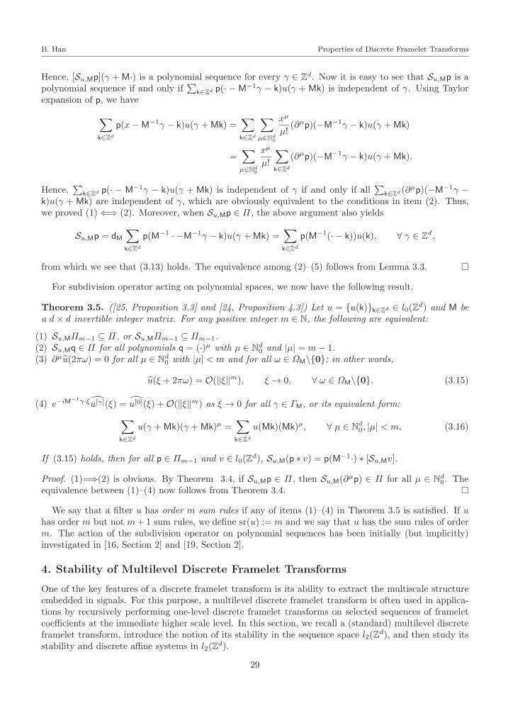
Hence, [Su,Mp](γ +M·) is a polynomial sequence for every γ ∈ Zd. Now it is easy to see that Su,Mp is apolynomial sequence if and only if
∑k∈Zd p(· −M−1γ − k)u(γ +Mk) is independent of γ. Using Taylor
expansion of p, we have
∑
k∈Zd
p(x−M−1γ − k)u(γ +Mk) =∑
k∈Zd
∑
µ∈Nd0
xµ
µ!(∂µp)(−M−1γ − k)u(γ +Mk)
=∑
µ∈Nd0
xµ
µ!
∑
k∈Zd
(∂µp)(−M−1γ − k)u(γ +Mk).
Hence,∑
k∈Zd p(· − M−1γ − k)u(γ + Mk) is independent of γ if and only if all∑
k∈Zd(∂µp)(−M−1γ −k)u(γ + Mk) are independent of γ, which are obviously equivalent to the conditions in item (2). Thus,we proved (1) ⇐⇒ (2). Moreover, when Su,Mp ∈ Π, the above argument also yields
Su,Mp = dM∑
k∈Zd
p(M−1 · −M−1γ − k)u(γ +Mk) =∑
k∈Zd
p(M−1(· − k))u(k), ∀ γ ∈ Zd,
from which we see that (3.13) holds. The equivalence among (2)–(5) follows from Lemma 3.3.
For subdivision operator acting on polynomial spaces, we now have the following result.
Theorem 3.5. ([25, Proposition 3.3] and [24, Proposition 4.3]) Let u = u(k)k∈Zd ∈ l0(Zd) and M be
a d× d invertible integer matrix. For any positive integer m ∈ N, the following are equivalent:
(1) Su,MΠm−1 ⊆ Π, or Su,MΠm−1 ⊆ Πm−1.(2) Su,Mq ∈ Π for all polynomials q = (·)µ with µ ∈ Nd0 and |µ| = m− 1.(3) ∂µu(2πω) = 0 for all µ ∈ Nd0 with |µ| < m and for all ω ∈ ΩM\0; in other words,
u(ξ + 2πω) = O(‖ξ‖m), ξ → 0, ∀ ω ∈ ΩM\0. (3.15)
(4) e−iM−1γ·ξu[γ](ξ) = u[0](ξ) +O(‖ξ‖m) as ξ → 0 for all γ ∈ ΓM, or its equivalent form:
∑
k∈Zd
u(γ +Mk)(γ +Mk)µ =∑
k∈Zd
u(Mk)(Mk)µ, ∀ µ ∈ Nd0, |µ| < m. (3.16)
If (3.15) holds, then for all p ∈ Πm−1 and v ∈ l0(Zd), Su,M(p ∗ v) = p(M−1·) ∗ [Su,Mv].
Proof. (1)=⇒(2) is obvious. By Theorem 3.4, if Su,Mp ∈ Π, then Su,M(∂µp) ∈ Π for all µ ∈ Nd0. The
equivalence between (1)–(4) now follows from Theorem 3.4.
We say that a filter u has order m sum rules if any of items (1)–(4) in Theorem 3.5 is satisfied. If uhas order m but not m+1 sum rules, we define sr(u) := m and we say that u has the sum rules of orderm. The action of the subdivision operator on polynomial sequences has been initially (but implicitly)investigated in [16, Section 2] and [19, Section 2].
4. Stability of Multilevel Discrete Framelet Transforms
One of the key features of a discrete framelet transform is its ability to extract the multiscale structureembedded in signals. For this purpose, a multilevel discrete framelet transform is often used in applica-tions by recursively performing one-level discrete framelet transforms on selected sequences of frameletcoefficients at the immediate higher scale level. In this section, we recall a (standard) multilevel discreteframelet transform, introduce the notion of its stability in the sequence space l2(Z
d), and then study itsstability and discrete affine systems in l2(Z
d).
29
“BinHan˙mmnp” — 2013/1/13 — 11:15 — page 30 — #13i
i
i
i
i
i
i
i
B. Han Properties of Discrete Framelet Transforms
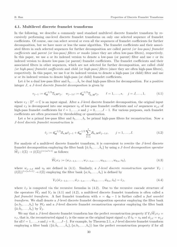
4.1. Multilevel discrete framelet transforms
In the following, we describe a commonly used standard multilevel discrete framelet transform by re-cursively performing one-level discrete framelet transforms on only one selected sequence of frameletcoefficients. Of course, one can select several or even all the sequences of framelet coefficients for furtherdecomposition, but we have more or less the same algorithm. The framelet coefficients and their associ-ated filters in such selected sequences for further decomposition are called parent (or low-pass) frameletcoefficients and parent (or low-pass) filters or masks (since they are often low-pass filters), respectively.In this paper, we use a or its indexed version to denote a low-pass (or parent) filter and use v or itsindexed version to denote low-pass (or parent) framelet coefficients. The framelet coefficients and theirassociated filters in other sequences, which are not selected for further decomposition, are called child(or high-pass) framelet coefficients and child (or high-pass) filters (since they are often high-pass filters),respectively. In this paper, we use b or its indexed version to denote a high-pass (or child) filter and usew or its indexed version to denote high-pass (or child) framelet coefficients.
Let a be a dual low-pass filter and b1, . . . , bs be dual high-pass filters for decomposition. For a positiveinteger J , a J-level discrete framelet decomposition is given by
vj−1 := d−1/2M Ta,Mvj , wj−1;ℓ := d
−1/2M Tbℓ,Mvj , ℓ = 1, . . . , s, j = J, . . . , 1, (4.1)
where vJ : Zd → C is an input signal. After a J-level discrete framelet decomposition, the original inputsignal vJ is decomposed into one sequence v0 of low-pass framelet coefficients and sJ sequences wj;ℓ ofhigh-pass framelet coefficients for ℓ = 1, . . . , s and j = 0, . . . , J − 1. For various purposes, such frameletcoefficients are often processed by thresholding or quantization.
Let a be a primal low-pass filter and b1, . . . , bs be primal high-pass filters for reconstruction. Now aJ-level discrete framelet reconstruction is
vj := d−1/2M Sa,Mvj−1 + d
−1/2M
s∑
ℓ=1
Sbℓ,Mwj−1;ℓ, j = 1, . . . , J. (4.2)
For analysis of a multilevel discrete framelet transform, it is convenient to rewrite the J-level discreteframelet decomposition employing the filter bank a; b1, . . . , bs by using a J-level decomposition operator
WJ : l(Z) → (l(Z))1×(sJ+1) as follows:
WJvJ := (wJ−1;1, . . . , wJ−1;s, . . . , w0;1, . . . , w0;s, v0), (4.3)
where wj−1;ℓ and v0 are defined in (4.1). Similarly, a J-level discrete reconstruction operator VJ :(l(Z))1×(sJ+1) → l(Z) employing the filter bank a; b1, . . . , bs is defined by
VJ(wJ−1;1, . . . , wJ−1;s, . . . , w0;1, . . . , w0;s, v0) = vJ , (4.4)
where vJ is computed via the recursive formulas in (4.2). Due to the recursive cascade structure of
the operators WJ and VJ in (4.1) and (4.2), a multilevel discrete framelet transform is often called afast framelet transform. A fast framelet transform with s = dM − 1 is further called a fast wavelettransform. We shall denote a J-level discrete framelet decomposition operator employing the filter banka; b1, . . . , bs by WJ and a J-level discrete framelet reconstruction operator employing the filter bank
a; b1, . . . , bs by VJ .
We say that a J-level discrete framelet transform has the perfect reconstruction property if VJWJvJ =vJ , that is, the reconstructed signal vJ is the same as the original input signal vJ if v0 = v0 and wj;ℓ = wj,ℓfor all ℓ = 1, . . . , s and j = 0, . . . , J−1. For example, by Theorem 2.1, a J-level discrete framelet transformemploying a filter bank (a; b1, . . . , bs, a; b1, . . . , bs) has the perfect reconstruction property if for all
30
“BinHan˙mmnp” — 2013/1/13 — 11:15 — page 31 — #14i
i
i
i
i
i
i
i
B. Han Properties of Discrete Framelet Transforms
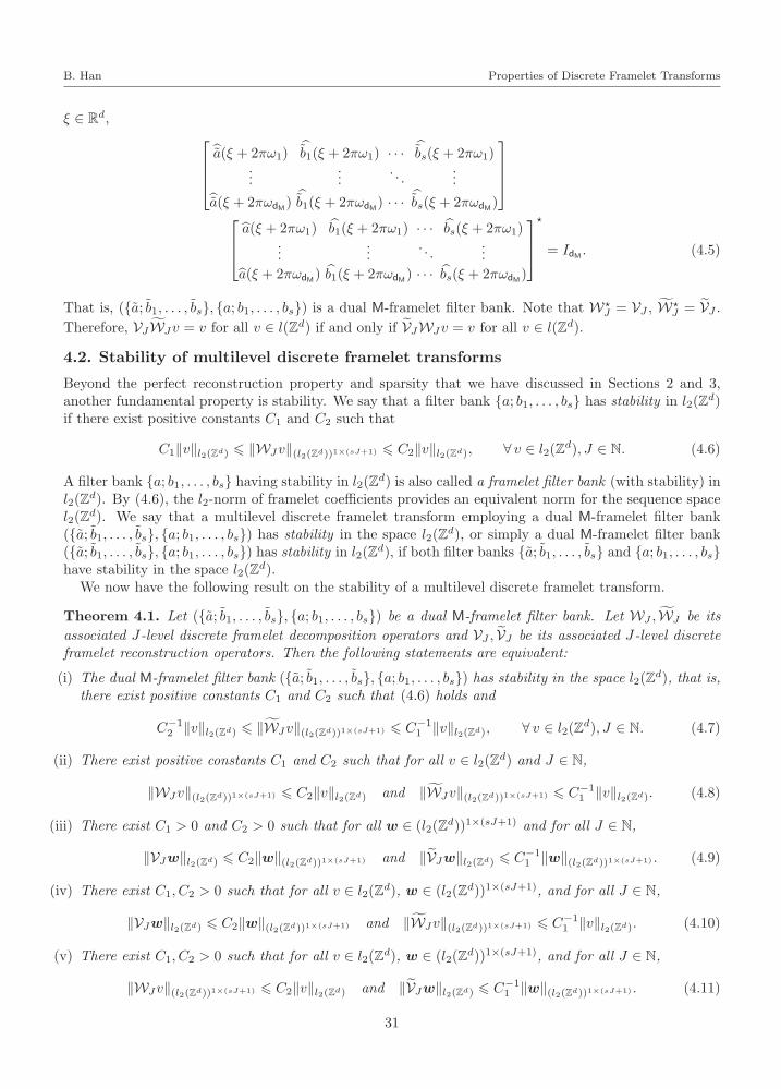
ξ ∈ Rd,
a(ξ + 2πω1)b1(ξ + 2πω1) · · ·
bs(ξ + 2πω1)
......
. . ....
a(ξ + 2πωdM)b1(ξ + 2πωdM) · · ·
bs(ξ + 2πωdM)
a(ξ + 2πω1) b1(ξ + 2πω1) · · · bs(ξ + 2πω1)
......
. . ....
a(ξ + 2πωdM) b1(ξ + 2πωdM) · · · bs(ξ + 2πωdM)
⋆
= IdM . (4.5)
That is, (a; b1, . . . , bs, a; b1, . . . , bs) is a dual M-framelet filter bank. Note that W⋆J = VJ , W
⋆J = VJ .
Therefore, VJWJv = v for all v ∈ l(Zd) if and only if VJWJv = v for all v ∈ l(Zd).
4.2. Stability of multilevel discrete framelet transforms
Beyond the perfect reconstruction property and sparsity that we have discussed in Sections 2 and 3,another fundamental property is stability. We say that a filter bank a; b1, . . . , bs has stability in l2(Z
d)if there exist positive constants C1 and C2 such that
C1‖v‖l2(Zd) 6 ‖WJv‖(l2(Zd))1×(sJ+1) 6 C2‖v‖l2(Zd), ∀ v ∈ l2(Zd), J ∈ N. (4.6)
A filter bank a; b1, . . . , bs having stability in l2(Zd) is also called a framelet filter bank (with stability) in
l2(Zd). By (4.6), the l2-norm of framelet coefficients provides an equivalent norm for the sequence space
l2(Zd). We say that a multilevel discrete framelet transform employing a dual M-framelet filter bank
(a; b1, . . . , bs, a; b1, . . . , bs) has stability in the space l2(Zd), or simply a dual M-framelet filter bank
(a; b1, . . . , bs, a; b1, . . . , bs) has stability in l2(Zd), if both filter banks a; b1, . . . , bs and a; b1, . . . , bs
have stability in the space l2(Zd).
We now have the following result on the stability of a multilevel discrete framelet transform.
Theorem 4.1. Let (a; b1, . . . , bs, a; b1, . . . , bs) be a dual M-framelet filter bank. Let WJ , WJ be its
associated J-level discrete framelet decomposition operators and VJ , VJ be its associated J-level discreteframelet reconstruction operators. Then the following statements are equivalent:
(i) The dual M-framelet filter bank (a; b1, . . . , bs, a; b1, . . . , bs) has stability in the space l2(Zd), that is,
there exist positive constants C1 and C2 such that (4.6) holds and
C−12 ‖v‖l2(Zd) 6 ‖WJv‖(l2(Zd))1×(sJ+1) 6 C−1
1 ‖v‖l2(Zd), ∀ v ∈ l2(Zd), J ∈ N. (4.7)
(ii) There exist positive constants C1 and C2 such that for all v ∈ l2(Zd) and J ∈ N,
‖WJv‖(l2(Zd))1×(sJ+1) 6 C2‖v‖l2(Zd) and ‖WJv‖(l2(Zd))1×(sJ+1) 6 C−11 ‖v‖l2(Zd). (4.8)
(iii) There exist C1 > 0 and C2 > 0 such that for all w ∈ (l2(Zd))1×(sJ+1) and for all J ∈ N,
‖VJw‖l2(Zd) 6 C2‖w‖(l2(Zd))1×(sJ+1) and ‖VJw‖l2(Zd) 6 C−11 ‖w‖(l2(Zd))1×(sJ+1) . (4.9)
(iv) There exist C1, C2 > 0 such that for all v ∈ l2(Zd), w ∈ (l2(Z
d))1×(sJ+1), and for all J ∈ N,
‖VJw‖l2(Zd) 6 C2‖w‖(l2(Zd))1×(sJ+1) and ‖WJv‖(l2(Zd))1×(sJ+1) 6 C−11 ‖v‖l2(Zd). (4.10)
(v) There exist C1, C2 > 0 such that for all v ∈ l2(Zd), w ∈ (l2(Z
d))1×(sJ+1), and for all J ∈ N,
‖WJv‖(l2(Zd))1×(sJ+1) 6 C2‖v‖l2(Zd) and ‖VJw‖l2(Zd) 6 C−11 ‖w‖(l2(Zd))1×(sJ+1) . (4.11)
31
“BinHan˙mmnp” — 2013/1/13 — 11:15 — page 32 — #15i
i
i
i
i
i
i
i
B. Han Properties of Discrete Framelet Transforms
If in addition s = dM − 1, any of the above statements is equivalent to
(vi) There exist positive constants C1 and C2 such that for all w ∈ (l2(Zd))1×(sJ+1) and J ∈ N,
C1‖w‖(l2(Zd))1×(sJ+1) 6 ‖VJw‖l2(Zd) 6 C2‖w‖(l2(Zd))1×(sJ+1) (4.12)
and
C−12 ‖w‖(l2(Zd))1×(sJ+1) 6 ‖VJw‖l2(Zd) 6 C−1
1 ‖w‖(l2(Zd))1×(sJ+1) . (4.13)
Proof. (i)=⇒(ii) is trivial. Note that VJ = W⋆J and VJ = W⋆
J . It follows from the well-known identities
‖W⋆J‖ = ‖WJ‖ and ‖W⋆
J‖ = ‖WJ‖ that (ii) ⇐⇒ (iii) ⇐⇒ (iv) ⇐⇒ (v), where ‖ · ‖ here refers to theoperator norm in the space l2(Z
d).
We now prove that (ii) and (iii) together imply (i). Since (a; b1, . . . , bs, a; b1, . . . , bs) is a dual M-
framelet filter bank, we have the perfect reconstruction property VJWJv = VJWJv = v for all v ∈ l2(Zd).
By (4.8) and (4.9), we have
‖v‖l2(Zd) = ‖VJWJv‖l2(Zd) 6 C−11 ‖WJv‖(l2(Zd))1×(sJ+1)
from which and (4.8) we see that (4.6) holds. (4.7) can be proved similarly.
Since v = VJWJv for all v ∈ l2(Zd), replacing ‖v‖l2(Zd) in (4.7) by ‖VJWJv‖l2(Zd), we deduce
C1‖WJv‖(l2(Zd))1×(sJ+1) 6 ‖VJWJv‖l2(Zd) 6 C2‖WJv‖(l2(Zd))1×(sJ+1) (4.14)
for all v ∈ l2(Zd) and J ∈ N. If s = dM − 1, then WJ is onto, and therefore, (4.12) follows directly from
(4.14). (4.13) can be proved similarly.
For VJ and VJ , generally we can only have (4.14) and its duality part by replacing WJ and VJ in (4.14)
with WJ and VJ , respectively. For s > dM, both (4.12) and (4.13) cannot hold, since by Proposition 2.2,there exists w 6≡ 0 in the space l0(Z
d) such that VJw = 0. Obviously, (4.10) implies that a small changeof an input data v induces a small change of all framelet coefficients, and a small perturbation of allframelet coefficients results in a small perturbation of a reconstructed signal. The notion of stability of amultilevel discrete framelet transform can be extended to other (weighted) sequence spaces and we shalladdress such issue elsewhere. Here we only provide some connections between stability of a multileveldiscrete framelet transform and a refinable function.
Proposition 4.2. Let a; b1, . . . , bs be a filter bank such that a(0) = 1 and there exists a positiveconstant C such that
‖WJv‖2(l2(Zd))1×(sJ+1) 6 C‖v‖2l2(Zd) ∀ v ∈ l2(Z
d), J ∈ N. (4.15)
Let M be a d × d expansive integer matrix, that is, all its eigenvalues are greater than one in modulus.Define a frequency-based refinable function ϕ by
ϕ(ξ) :=
∞∏
j=1
a((MT)−jξ), ξ ∈ Rd. (4.16)
Then ϕ ∈ L2(Rd) with ‖ϕ‖2L2(Rd) 6 (2π)dC.
Proof. Since VJ = W⋆J , by (4.15), we have
‖VJw‖2l2(Zd) 6 C‖w‖2(l2(Zd))1×(sJ+1) ∀ w ∈ (l2(Zd))1×(sJ+1), J ∈ N. (4.17)
32
“BinHan˙mmnp” — 2013/1/13 — 11:15 — page 33 — #16i
i
i
i
i
i
i
i
B. Han Properties of Discrete Framelet Transforms
Take w0 = (0, . . . , 0, δ), that is, v0 = δ and all high-pass framelet coefficients vanish. Then VJw0 =
d−J/2M SJa,Mδ. Since the Fourier series of SJa,Mδ is dJM
∏J−1j=0 a((M
T)jξ), we have
‖VJw0‖2l2(Zd) = ‖d
−J/2M SJa,Mδ‖
2l2(Zd) = d−JM ‖SJa,Mδ‖
2l2(Zd) =
dJM(2π)d
∫
[−π,π)d
J−1∏
j=0
|a((MT)jξ)|2dξ
=1
(2π)d
∫
Rd
χ(MT)J [−π,π)d(ξ)J∏
j=1
|a((MT)−jξ)|2dξ.
It now follows from ‖VJw0‖2l2(Zd) 6 C‖w0‖
2l2(Zd) = C that
1
(2π)d
∫
Rd
χ(MT)J [−π,π)d(ξ)J∏
j=1
|a((MT)−jξ)|2dξ = ‖d−J/2M SJa,Mδ‖
2l2(Zd) = ‖VJw0‖
2l2(Zd) 6 C.
Since M is expansive, we have limJ→∞ χ(MT)J [−π,π)d(ξ)∏Jj=1 |a((M
T)−jξ)|2 = |ϕ(ξ)|2 for all ξ ∈ Rd.Applying Fatou’s lemma, we have
1
(2π)d
∫
Rd
|ϕ(ξ)|2dξ 6 lim infJ→∞
1
(2π)d
∫
Rd
χ(MT)J [−π,π)d(ξ)J∏
j=1
|a((MT)−jξ)|2dξ 6 C.
Hence, ϕ ∈ L2(Rd) and ‖ϕ‖2L2(Rd) 6 (2π)dC.
4.3. Discrete affine systems for l2(Zd)
In this section, we explain the role played by the dilation matrix M in a multilevel discrete framelettransform. Then we give the definition of discrete affine systems for l2(Z
d). In other words, we introducethe notion of discrete framelets and discrete wavelets for l2(Z
d) in this section.To implement the subdivision and transition operators using the convolution operation, we need the
upsampling and downsampling operators on sequences in l(Zd). The upsampling operator ↑M : l(Zd) →l(Zd) and the downsampling (or decimation) operator ↓M : l(Zd) → l(Zd) with a d× d sampling matrixM are defined to be
[v↑M](n) :=
v(M−1n), if n ∈ MZd;
0, otherwise,and [v↓M](n) := v(Mn), n ∈ Zd. (4.18)
It is convenient to use the notation v(M−1·) for v↑M and v(M·) for v↓M. Now the subdivision operatorSu,M in (2.1) and the transition operator Tu,M in (2.2) can be equivalently expressed as follows:
Su,Mv = dMu ∗ (v↑M) and Tu,Mv = dM(u⋆ ∗ v)↓M. (4.19)
According to (4.19), the subdivision and transition operators differ to the convolution operation only inthe use of the upsampling and downsampling operators with the sampling matrix M, which plays a crucialrole in a multilevel discrete framelet transform to extract multiscale structure embedded in a signal. Tounderstand this point well, instead of viewing the decomposition operator WJ and the reconstructionoperator VJ in the recursive way as in (4.1) and (4.2), we consider wj;ℓ as a direct consequence of a linearmapping acting on the input signal v (more precisely, vJ).
We have the following result on the recursive application of subdivision or transition operators.
Lemma 4.3. Let M1,M2 be d× d invertible integer matrices and let u1, u2 ∈ l0(Zd). Then
Su1,M1Su2,M2
v = Su1∗(u2↑M1),M1M2v = | det(M1M2)|u1 ∗ (u2 ↑M1) ∗ (v↑M1M2) (4.20)
andTu2,M2
Tu1,M1v = Tu1∗(u2↑M1),M1M2
v = | det(M1M2)|(u1 ∗ (u2 ↑M1) ∗ v)↓M1M2. (4.21)
33
“BinHan˙mmnp” — 2013/1/13 — 11:15 — page 34 — #17i
i
i
i
i
i
i
i
B. Han Properties of Discrete Framelet Transforms
Proof. The Fourier series of the sequence Su1,M1Su2,M2
v is
| det(M1)|u1(ξ)Su2,M2v(MT
1 ξ) = | det(M1M2)|u1(ξ)u2(MT1 ξ)v(M
T2M
T1 ξ).
Therefore, (4.20) holds. By duality in (2.18) and by (4.20), we have
〈w, Tu2,M2Tu1,M1
v〉 = 〈Su2,M2w, Tu1,M1
v〉 = 〈Su1,M1Su2,M2
w, v〉
= 〈Su1∗(u2↑M1),M1M2w, v〉 = 〈w, Tu1∗(u2↑M1),M1M2
v〉,
from which we see that (4.21) holds.
From the definition of the sequence wj;ℓ of framelet coefficients in (4.1), we see that
vj = d−1/2M Ta,Mvj+1 = · · · = d
(j−J)/2M T J−j
a,M vJ = d(j−J)/2M Ta∗(a↑M)∗···∗(a↑MJ−j−1),MJ−jv (4.22)
and
wj;ℓ = d−1/2M Tbℓvj+1 = d
(j−J)/2M Tbℓ,MT
(j+1−J)/2a,M vJ = d
(j−J)/2M Ta∗(a↑M)∗···∗(a↑MJ−j−2)∗(bℓ↑MJ−j−1),MJ−jv.
Therefore, framelet coefficients wj−1;ℓ are obtained by filtering a given signal v using the filters d(J−j)/2M a∗
(a ↑ M)∗ · · · ∗ (a ↑ MJ−j−1)∗ (bℓ ↑ MJ−j), whose supports grow with the scale level J − j. More precisely,by (2.2),
wj;ℓ(k) =⟨v, d
(J−j)/2M [a ∗ (a↑M) ∗ · · · ∗ (a↑MJ−j−2) ∗ (bℓ ↑M
J−j−1)](· −MJ−jk)⟩, k ∈ Zd.
Similarly, we deduce that
VJ (0, . . . , 0, v0) = d−J/2M SJa,Mv0 = d
(j−J)/2M Sa∗(a↑M)∗···∗(a↑MJ−1),MJ v0 (4.23)
and
VJ(0, . . . , 0, wj;ℓ, 0, . . . , 0) = d(j−J)/2M SJ−j−1
a,M Sbℓ,Mwj;ℓ
= d(j−J)/2M Sa∗(a↑M)∗···∗(a↑MJ−j−2)∗(bℓ↑MJ−j−1),MJ−jwj;ℓ. (4.24)
Define filters aj and aj , j ∈ N by
aj(ξ) := a(ξ)a(MTξ) · · · a((MT)j−1ξ) and aj(ξ) := a(ξ)a(MTξ) · · · a((MT)j−1ξ) (4.25)
with the convention that a0 = a0 := δ. That is,
aj = a ∗ (a↑M) ∗ · · · ∗ (a↑Mj−1) and aj := a ∗ (a↑M) ∗ · · · ∗ (a↑Mj−1). (4.26)
Now a J-level discrete framelet transform employing a dual M-framelet filter bank (a; b1, . . . , bs,a; b1, . . . , bs) can be equivalently rewritten as
v =∑
k∈Zd
〈v, a[J;k]〉a[J;k] +
J∑
j=1
∑
k∈Zd
s∑
ℓ=1
〈v, bℓ,[j;k]〉bℓ,[j;k], (4.27)
wherea[j;k] := d
j/2M aj(· −Mjk), bℓ,[j;k] := d
j/2M [aj−1 ∗ (bℓ ↑M
j−1)](· −Mjk) (4.28)
anda[j;k] := d
j/2M aj(· −Mjk), bℓ,[j;k] := d
j/2M [aj−1 ∗ (bℓ ↑M
j−1)](· −Mjk). (4.29)
34

“BinHan˙mmnp” — 2013/1/13 — 11:15 — page 35 — #18i
i
i
i
i
i
i
i
B. Han Properties of Discrete Framelet Transforms
By employing the dilation matrix M, a multilevel discrete framelet transform provides a multi-scale rep-resentation of a signal, which is the key to extract the multiscale structure in a signal. The representationin (4.27) also shows that the stability of a multilevel discrete framelet transform in the space l2(Z
d) isclosely related to the asymptotic behavior of the sequences aJ , aJ in (4.25) as J → +∞, which is in turnclosely related to the frequency-based refinable functions ϕ and ϕ.
The above discussion motivates us to define discrete affine systems as follows:
DASJ(a; b1, . . . , bs) :=a[J;k] : k ∈ Zd
∪ bℓ,[j;k] : ℓ = 1, . . . , s, j = 1, . . . , J, k ∈ Zd (4.30)
and
DASJ (a; b1, . . . , bs) :=a[J;k] : k ∈ Zd
∪ bℓ,[j;k] : ℓ = 1, . . . , s, j = 1, . . . , J, k ∈ Zd. (4.31)
Under the convention that
∼ : DASJ(a; b1, . . . , bs) → DASJ(a; b1, . . . , bs) with u 7→ u,
that is, (u, u) is always regarded as a pair together, the representation of v ∈ l2(Zd) in (4.27) can be
rewritten asv =
∑
u∈DASJ (a;b1,...,bs)〈v, u〉u, v ∈ l2(Z
d), J ∈ N. (4.32)
Therefore, the stability in (4.6) of a filter bank a; b1, . . . , bs in l2(Zd) simply means the stability of the
discrete affine system DASJ (a; b1, . . . , bs) in l2(Zd):
C21‖v‖
2l2(Zd) 6
∑
u∈DASJ (a;b1,...,bs)|〈v, u〉|2 6 C2
2‖v‖2l2(Zd), ∀ v ∈ l2(Z
d), J ∈ N. (4.33)
In other words, if a; b1, . . . , bs has stability in l2(Zd) , then DASJ(a; b1, . . . , bs) is a frame for L2(R
d)for all J ∈ N. It is also easy to prove that a; b1, . . . , bs is a tight M-framelet filter bank if and only if(4.33) holds with C1 = C2 = 1. Furthermore, a; b1, . . . , bdM is an orthogonal M-wavelet filter bank ifand only if DASJ (a; b1, . . . , bdM) is an orthonormal basis for l2(Z
d) for every J ∈ N.
4.4. Variants of multilevel discrete framelet transforms
There are many variants to a standard multilevel discrete framelet transform. Here we look at twoparticular variants. By the definition in (2.1) and (2.2), it is easy to notice that
Su,M(v(· − n)) = [Su,Mv](· −Mn), Su(·−n),Mv = [Su,Mv](· − n), n ∈ Zd (4.34)
andTu,M(v(· −Mn)) = [Tu,Mv](· − n), Tu(·+n),Mv = Tu,M(v(· − n)), n ∈ Zd. (4.35)
In other words, if we shift an input signal v or a filter u by an integer, then its output under the subdivisionoperator is a shifted version of Su,Mv. For the transition operator, however, Tu,M(v(· − n)) or Tu(·+n),Mvis generally no longer a shifted version of Tu,Mv if n 6∈ MZd. This shift sensitivity of framelet coefficientswith respect to a shift of an input signal is not desirable in some applications such as signal or imagedenoising, since a simple shift of a noise wouldn’t change the characteristics of a noise. To overcome thisdifficulty, we put together the dM sequences Tu(·+γ),Mv, γ ∈ ΓM in a disjoint way so that we have onlyone sequence dMu
⋆ ∗ v. Similarly, it is easy to verify that∑γ∈ΓM
Su(·+γ),M(w(M · −γ)) = dMu ∗ w. Inother words, the new discrete framelet transform is undecimated by removing the downsampling (i.e.,decimation) and upsampling operations in the original discrete framelet transform. Thus, it is called a
35
“BinHan˙mmnp” — 2013/1/13 — 11:15 — page 36 — #19i
i
i
i
i
i
i
i
B. Han Properties of Discrete Framelet Transforms
J-level discrete undecimated framelet transform employing the filter bank (a; b1, . . . , bs, a; b1, . . . , bs),which in the terminology of Subsection 4.1 is just a J-level discrete framelet transform employing thenew filter bank
(d−1/2M a(· − γ1), . . . , a(· − γdM); b1(· − γ1), . . . , b1(· − γdM), . . . , bs(· − γ1), . . . , bs(· − γdM),
d−1/2M a(· − γ1), . . . , a(· − γdM); b1(· − γ1), . . . , b1(· − γdM), . . . , bs(· − γ1), . . . , bs(· − γdM)),
where γ1, . . . , γdM := ΓM. Let us present a J-level discrete undecimated framelet transform employinga dual M-framelet filter bank (a; b1, . . . , bs, a; b1, . . . , bs). A J-level discrete undecimated frameletdecomposition is given by
vj−1 := (a⋆ ↑MJ−j) ∗ vj , wj−1;ℓ := (b⋆ℓ ↑MJ−j) ∗ vj , ℓ = 1, . . . , s, j = J, . . . , 1, (4.36)
where vJ : Zd → C is an input signal. A J-level discrete undecimated framelet reconstruction is
vj := (a↑MJ−j) ∗ vj−1 +
s∑
ℓ=1
(bℓ ↑MJ−j) ∗ wj−1;ℓ, j = 1, . . . , J. (4.37)
Using the same proof as in Theorem 2.1, one can straightforwardly check that the above J-level discreteundecimated framelet transform has the perfect reconstruction property if and only if
a(ξ)a(ξ) + b1(ξ)b1(ξ) + · · ·+
bs(ξ)bs(ξ) = 1. (4.38)
Therefore, the perfect reconstruction condition on a filter bank for an undecimated framelet transformis much weaker than the condition in (4.5) for an usual dual M-framelet filter bank. In this sense, anundecimated framelet transform would be properly called a multiscale convolution transform using a filterbank satisfying (4.38). Similar to (4.27), we have the signal representation:
v =∑
k∈Zd
⟨v, aJ (· − k)
⟩aJ(· − k) +
J∑
j=1
∑
k∈Zd
s∑
ℓ=1
〈v, bℓ,[j;0](· − k)〉bℓ,[j;0](· − k). (4.39)
A J-level discrete undecimated framelet transform has redundancy ratio Js while the original J-level
discrete framelet transform has redundancy ratios(dJ−1
M−1)
dJ−1M
(dM−1)+ 1
dJ−1M
(a J-level discrete wavelet transform
has redundancy ratio one, that is, no redundancy). Therefore, a J-level discrete undecimated framelettransform is a redundant transform, having roughly dMJ times more coefficients than the original J-leveldiscrete framelet transform, but has a simple structure. To reduce the redundancy rate and to keep thetransform nearly shift invariant, we discuss another variant—a discrete averaging framelet transform.
Let n be a positive integer. We say that A := (A1, . . . ,An) : l(Zd) → (l(Zd))1×n,Av = (A1v, . . . ,Anv)
is a data partitioning operator if A is an injective operator (that is, a one-to-one but not necessarily linearmapping). A has at least one left-inverse and we say that A : (l(Zd))1×n → l(Zd) is a data averagingoperator of A if AAv = v for all v ∈ l(Zd). An example of data partitioning and data averaging operatorsis to use the convolution operation. Let Θ1, . . . , Θn, Θ1, . . . , Θn ∈ l0(Z) be finitely supported sequenceson Zd such that
Θ1(ξ)Θ1(ξ) + · · ·+ Θn(ξ)Θn(ξ) = 1. (4.40)
Then we have a data partitioning operator A : l(Zd) → (l(Zd))1×n,Av = (Θ⋆1 ∗ v, . . . , Θ⋆n ∗ v) and a data
averaging operator A : (l(Zd))1×n → l(Zd), A(v1, . . . , vn) = Θ1 ∗v1+ · · ·+ Θn ∗vn. By (4.40), it is evidentthat AA = Idl(Zd). A simple choice is to take Θ1 = · · · = Θn = δ and Θ1 = · · · = Θn = 1
nδ. For thisparticular example, the data partitioning operator simply copies the data n times and the data averagingoperator A is exactly the averaging operation.
Under a data partitioning operator A, a signal v is split into n sub-signals: A1v, . . . ,Anv. Regard eachsub-signal as a completely separate branch. Now a discrete n-branch averaging framelet transform is to
36
“BinHan˙mmnp” — 2013/1/13 — 11:15 — page 37 — #20i
i
i
i
i
i
i
i
B. Han Properties of Discrete Framelet Transforms
perform an independent discrete framelet transform on each branch. After processing and reconstructionof each branch, we end up with n reconstructed sub-signals. Then we use the data averaging operator toform one reconstructed signal.
A particular discrete framelet transform may perform better only for a small subset of signals withcertain characteristics. Using a data partitioning operator, we may be able to split a signal into sub-signals with different characteristics so that the advantages of a particular discrete framelet transform canbe explored. Comparing with a J-level discrete undecimated framelet transform which has redundancyratio Js, a J-level discrete n-branch averaging framelet transform has only n times redundancy, whichis independent of the scale level J and is much smaller than Js when the scale level J is large. Adiscrete averaging framelet transform using complex-valued dual framelet filter banks is of particularinterest in high-dimensional data analysis for achieving directional representations to capture varioushigh-dimensional singularities such as edges in images. For example, the dual-tree complex wavelettransform employing two correlated orthogonal wavelet filter banks (see the tutorial article [38]) is aparticular example of the averaging framelet transform with n = 2 branches. See Section 7 for anotherexample of directional framelets using tensor product complex-valued tight framelet filter banks.
5. Linear-phase Moments and Symmetry Property of Framelets
In this section we discuss linear-phase moments and symmetry property in wavelet analysis.It is sometimes desirable that the image of a polynomial under a convolution operation is itself or its
translated version. For this purpose, we recall the notion of linear-phase moments introduced in [23,26].We say that u ∈ l0(Z
d) has order m linear-phase moments with phase c ∈ Rd if
u(ξ) = e−ic·ξ +O(‖ξ‖m), ξ → 0. (5.1)
If m > 1, it follows from (5.1) that c =∑
k∈Zd u(k)k, which is called the default phase of u. If u has orderm but not m+ 1 linear-phase moments with the default phase, then we define lpm(u) := m and we saythat u has the linear-phase moments of order m.
If a filter has linear-phase moments, then the action of the convolution operation, the subdivisionoperator, and the transition operator on polynomial spaces has some particular structure.
Proposition 5.1. Let u ∈ l0(Zd), c ∈ Rd, and m ∈ N0. Then (i) p ∗ u = p(· − c) for all p ∈ Πm−1 if
and only if (ii) u has order m linear-phase moments with phase c if and only if (iii) Tu,Mp = dMp(M ·+c)for all p ∈ Πm−1. Similarly, u has order m sum rules and order m linear-phase moments with phase c
if and only if Su,Mp = p(M−1(· − c)) for all p ∈ Πm−1.
Proof. By Lemma 3.1, we have (3.7). On the other hand, using the Taylor expansion of p, we have
p(x − c) =∑µ∈Nd
0 ,|µ|<m ∂µp(x) (−c)µ
µ! . Comparing the coefficients of ∂µp, µ ∈ Nd0, |µ| < m with (3.7), we
see that p ∗ u = p(· − c) if and only if ∂µu(0) = (−ic)µ for all µ ∈ Nd0, |µ| < m, which can be equivalentlyrewritten as (5.1). (iii) is a direct consequence of item (i) and (3.10) in Theorem 3.2. The part onsubdivision operator is a direct consequence of Theorem 3.5.
Linear-phase moments are of particular interest in the application of subdivision schemes in computeraided geometric design, since the property Su,Mp = p(M−1(· − c)) for all p ∈ Πm−1 simply means thatthe subdivision scheme is interpolating on all polynomial sequences p ∈ Πm−1.
In the following, we make some remarks on the relations between linear-phase moments and symmetry.Note that a filter u has one linear-phase moment just means u(0) = 1.
Proposition 5.2. Let u ∈ l0(Zd) satisfying lpm(u) > 1 with phase c ∈ Rd.
(i) If u(cu − k) = u(k) for all k ∈ Zd with cu ∈ Zd, then c = cu/2 (that is, the phase c agrees with thesymmetry center cu/2 of u) and lpm(u) must be an even integer;
(ii) If u(cu − k) = u(k) for all k ∈ Zd with cu ∈ Zd, then c = cu/2.
37
“BinHan˙mmnp” — 2013/1/13 — 11:15 — page 38 — #21i
i
i
i
i
i
i
i
B. Han Properties of Discrete Framelet Transforms
Proof. Set m := lpm(u). For (i), we have u(ξ) = e−icu·ξu(−ξ). Then it follows from (5.1) that e−icu·ξ =u(ξ)u(−ξ) = e−i2c·ξ+O(‖ξ‖m) as ξ → 0. Since m > 1, we must have c = cu/2. Note that u(ξ) = e−icu·ξu(−ξ)
and cu = 2c imply u(ξ)eic·ξ = u(−ξ)e−ic·ξ, from which we see that
∂µ[u(ξ)eic·ξ](0) = 0, for all µ ∈ Nd0 with positive odd integers |µ|. (5.2)
On the other hand, the definition of linear-phase moments in (5.1) is equivalent to u(ξ)eic·ξ = 1+O(‖ξ‖m)as ξ → 0. Since u has m but not m + 1 linear-phase moments with phase c, it now follows from (5.2)that m must be an even integer.
For (ii), we have u(ξ) = e−icu·ξu(ξ). Then it follows from (5.1) that we must have e−icu·ξ = u(ξ)
u(ξ)=
e−i2c·ξ +O(‖ξ‖m) as ξ → 0. Thus, c = cu/2 holds.
According to the following result, linear-phase moments also play a critical role in the construction oftight framelet filter banks having symmetry.
Proposition 5.3. Let a; b1, . . . , bs be a tight M-framelet filter bank such that a(0) = 1 and a(ca− k) =a(k) for all k ∈ Zd with ca ∈ Zd. Then lpm(a⋆ ∗ a) = lpm(a) and
min(vm(b1), . . . , vm(bs)) = min(sr(a), 12 lpm(a)). (5.3)
Proof. By a(0) = 1 we see from the perfect reconstruction condition (4.5) (also see [4, 10]) that
min(vm(b1), . . . , vm(bs)) = min(sr(a),1
2vm(1− |a|2)). (5.4)
Since a has symmetry, we have a(ξ) = e−ica·ξa(ξ). Set c := ca/2 and n := vm(1− |a|2) Then,
[1 + eic·ξa(ξ)][1− eic·ξa(ξ)] = 1− |a(ξ)|2 = O(‖ξ‖n), ξ → 0.
Since a(0) = 1, we conclude from the above relation that 1 − eic·ξa(ξ) = O(‖ξ‖n) as ξ → 0. That is,we proved lpm(a) > n. It is trivial that vm(1 − |a|2) > lpm(a). Note that vm(1 − |a|2) = lpm(a⋆ ∗ a).Hence, lpm(a⋆ ∗ a) = lpm(a) and (5.3) follows directly from (5.4).
We now discuss symmetry properties of wavelets and framelets which are desirable in many appli-cations. Let G be a finite subset of d × d integer matrices whose determinants are ±1. We say thatG is a symmetry group compatible with a d × d invertible integer matrix M (see [17, 18, 21, 22]) if G
forms a group under matrix multiplication and M−1EM ∈ G for all E ∈ G . That is, the mappinggM : G → G , gM(E) := M−1EM is well defined. Note that g−1
M (E) = MEM−1. For matrices M and N, wesay that N is G -equivalent to M if N = EMF for some E,F ∈ G . Note that Id,−Id is a basic symmetrygroup compatible with any d× d invertible integer matrix M. In dimension two, there are two importantsymmetry groups:
D4 :=
±
[1 00 1
],±
[1 00 −1
],±
[0 11 0
],±
[0 1−1 0
], (5.5)
D6 :=
±
[1 00 1
],±
[0 −11 −1
],±
[−1 1−1 0
],±
[0 11 0
],±
[1 −10 −1
],±
[−1 0−1 1
]. (5.6)
Define
M√2 :=
[1 11 −1
], M√
3 :=
[1 −22 −1
], I2 :=
[1 00 1
]. (5.7)
As shown in [21, Theorem 2], up to D4-equivalence and a multiplicative constant, M√2 and I2 are the
only two matrices which are compatible with D4. Similarly, up to D6-equivalence and a multiplicativeconstant, M√
3 and I2 are the only two matrices which are compatible with D6.
38
“BinHan˙mmnp” — 2013/1/13 — 11:15 — page 39 — #22i
i
i
i
i
i
i
i
B. Han Properties of Discrete Framelet Transforms
Let a ∈ l0(Zd) and G be a symmetry group on Zd. We say that a has G -symmetry with a symmetry
center ca ∈ Rd and ǫa ∈ −1, 1 if
a(E(k− ca) + ca) = ǫaa(k), ∀ k ∈ Zd, E ∈ G . (5.8)
Clearly, we must have (Id − E)ca ∈ Zd for all E ∈ G . Similarly, we say that a has complex G -symmetrywith a symmetry center ca ∈ Rd and ǫa ∈ −1, 1 if
a(E(k− ca) + ca) = ǫaa(k), ∀ k ∈ Zd, E ∈ G . (5.9)
Now we have the following result on symmetry of an M-refinable function and its mask.
Theorem 5.4. ([22, Proposition 2.1]) Let M be a d× d expansive integer matrix. Let G be a symmetrygroup compatible with M. Let a ∈ l0(Z
d) with a(0) = 1. Define ϕ as in (4.16) and a compactly supported
distribution φ by φ = ϕ, that is, φ(x) = 1(2π)d
∫Rd ϕ(ξ)e
ix·ξdξ if ϕ ∈ L1(Rd). Then a has G -symmetry
with a symmetry center ca and ǫa = 1 if and only if
φ(E(· − cφ) + cφ) = φ, ∀ E ∈ G with cφ := (M− Id)−1ca. (5.10)
Moreover, if N = EMF for some E,F ∈ G (that is, N is G -equivalent to M), then N is also expansive,φN = φ(·+ (M− Id)
−1ca − (N− Id)−1ca), and
φN(E(· − cN) + cN) = φN, ∀ E ∈ G . (5.11)
where cN := (N − Id)−1ca and φN(ξ) :=
∏∞j=1 a((N
T)−jξ), ξ ∈ Rd. If b ∈ l0(Zd) and Gb is a subgroup of
G such that b has Gb-symmetry with a symmetry center cb and ǫb ∈ −1, 1, then
ψ(F (· − cψ) + cψ) = ǫbψ, ∀ F ∈ Gb with cψ := M−1cb +M−1(M− Id)−1ca, (5.12)
where ψ := dM∑
k∈Zd b(k)φ(M · −k), that is, ψ(MTξ) := b(ξ)φ(ξ). If G -symmetry and Gb-symmetryare replaced by complex G -symmetry and complex Gb-symmetry, respectively, then all the claims hold byadding complex conjugate to the right sides of (5.10), (5.11), and (5.12).
Proof. Note that (5.10) is equivalent to
φ(ETξ) = ei(ca−Eca)·ξφ(ξ) = ei(Id−E)(M−Id)−1ca·ξφ(ξ), ∀ E ∈ G , ξ ∈ Rd. (5.13)
Also note that (5.8) holds if and only if
a(ETξ) = ǫaei(Id−E)ca·ξa(ξ), E ∈ G , ξ ∈ Rd. (5.14)
By the definition of φ in (4.16) and the relation φ(MTξ) = a(ξ)φ(ξ), one can easily check that (5.14)holds if and only if (5.13) holds.
Since G is finite and limj→∞ M−j = 0, we must have limj→∞ N−j = 0. By the definition of φ and
φN, we can directly check that φN(ξ) = ei[(M−Id)−1−(N−Id)−1]ca·ξφ(ξ) is satisfied and (5.11) holds. Using
(5.13) and b(FTξ) = ǫbei(Id−F )ca·ξ b(ξ) for all F ∈ Gb, we have (5.12).
6. Connections of Filter Banks to Frequency-based Dual Framelets
In this section we discuss the connections between dual framelet filter banks and frequency-based dualframelets. We shall see that every dual framelet filter bank (a; b1, . . . , bs, a; b1, . . . , bs) satisfyinga(0) = a(0) = 1 corresponds to a frequency-based dual framelet on Rd, which is introduced in [27, 28].For simplicity of presentation, we only outline the main ideas of the proofs and refer the reader to [27,28]for the detailed proofs of the results stated in this section. At the end of this section, we mention some
39
“BinHan˙mmnp” — 2013/1/13 — 11:15 — page 40 — #23i
i
i
i
i
i
i
i
B. Han Properties of Discrete Framelet Transforms
connections between the sparsity of a discrete framelet transform and the sparse representation of a dualframelet in the function space L2(R
d).Following the standard notation, we denote by D(Rd) the linear space of all compactly supported
C∞ functions. By Llocp (Rd) we denote the linear space of all measurable functions f such that∫y∈Rd : ‖y‖6r |f(x)|
pdx < ∞ for all r > 0 with the usual modification for p = ∞. For f ∈ D(Rd)
and ψ ∈ Lloc1 (Rd), we shall use the following pairing
〈f ,ψ〉 :=
∫
Rd
f(ξ)ψ(ξ)dξ and 〈ψ, f〉 := 〈f ,ψ〉 =
∫
Rd
ψ(ξ)f(ξ)dξ.
Let J be an integer and N be a d× d invertible real-valued matrix. Let Φ and Ψ be subsets of Lloc1 (Rd).A frequency-based (NT)−1-affine system (or an N-modulation system) is defined to be
FASJ(Φ;Ψ) = ϕNJ ;0,k : k ∈ Zd,ϕ ∈ Φ ∪ ∪∞j=JψNj ;0,k : k ∈ Zd,ψ ∈ Ψ, (6.1)
where we used the notation in (1.1). To emphasize the role played by N, we also use FASNJ (Φ;Ψ) insteadof FASJ(Φ;Ψ). Let
Φ = ϕ1, . . . ,ϕr, Φ = ϕ1, . . . , ϕr, Ψ = ψ1, . . . ,ψs, Ψ = ψ1, . . . , ψs (6.2)
be subsets of Lloc1 (Rd). Let FASJ(Φ;Ψ) be defined in (6.1) and FASJ(Φ; Ψ ) be defined similarly. As in[27, 28], we say that the pair (FASJ(Φ;Ψ),FASJ(Φ; Ψ )) is a frequency-based dual (NT)−1-framelet if thefollowing identity holds
r∑
ℓ=1
∑
k∈Zd
〈f ,ϕℓNJ ;0,k〉〈ϕℓNJ ;0,k,g〉+
∞∑
j=J
s∑
ℓ=1
∑
k∈Zd
〈f ,ψℓNj ;0,k〉〈ψℓNj ;0,k,g〉 = (2π)d〈f ,g〉 (6.3)
for all f ,g ∈ D(Rd), where the infinite series in (6.3) converge in the following sense
(i) for every f ,g ∈ D(Rd), all the following series converge absolutely for all integers j > J :
r∑
ℓ=1
∑
k∈Zd
〈f ,ϕℓNJ ;0,k〉〈ϕℓNJ ;0,k,g〉 and
s∑
ℓ=1
∑
k∈Zd
〈f ,ψℓNj ;0,k〉〈ψℓNj ;0,k,g〉. (6.4)
(ii) for every f ,g ∈ D(Rd), the following limit exists and
limn→+∞
( r∑
ℓ=1
∑
k∈Zd
〈f ,ϕℓNJ ;0,k〉〈ϕℓNJ ;0,k,g〉
+
n−1∑
j=J
s∑
ℓ=1
∑
k∈Zd
〈f ,ψℓNj ;0,k〉〈ψℓNj ;0,k,g〉
)= (2π)d〈f ,g〉. (6.5)
As shown in [27, Lemma 3] and [28, Lemma 10], the condition in the above item (i) is automaticallysatisfied if Φ,Ψ , Φ, Ψ are subsets of Lloc2 (Rd) and r, s are finite integers. The condition in the aboveitem (ii) is simply the perfect reconstruction property in the test function space D(Rd) for a pair offrequency-based affine systems.
Let J be an integer and M be a d×d invertible real-valued matrix. Let Φ and Ψ be subsets of Lloc1 (Rd).A nonhomogeneous M-affine system is defined to be
ASJ (Φ;Ψ) = φMJ ;k : k ∈ Zd, φ ∈ Φ ∪ ∪∞j=JψMj ;k : k ∈ Zd, ψ ∈ Ψ. (6.6)
To emphasize the role played by M, we also use ASMJ (Φ;Ψ) instead of ASJ (Φ;Ψ). If Φ, Ψ are subsets of
L2(Rd), then we can define Φ := φ : φ ∈ Φ and Ψ := ψ : ψ ∈ Ψ, where the Fourier transform used
40
“BinHan˙mmnp” — 2013/1/13 — 11:15 — page 41 — #24i
i
i
i
i
i
i
i
B. Han Properties of Discrete Framelet Transforms
in this paper is defined to be f(ξ) :=∫Rd f(x)e
−ix·ξdx, ξ ∈ Rd for f ∈ L1(Rd). Then it is easy to see that
the image of ASMJ (Φ;Ψ) under the Fourier transform is exactly FASNJ (Φ,Ψ) with N = (MT)−1. Moreover,the homogeneous M-affine system AS(Ψ) in (1.2) is simply the limiting system of ASJ (Φ, Ψ) as J → −∞.See [27,28] for more detail.
Frequency-based dual framelets can be completely characterized as follows:
Theorem 6.1. ([28, Theorem 11] and [27, Theorem 6]) Let M be a d × d real-valued invertible matrixsuch that M is expansive. Define N := (MT)−1. Let Φ, Φ,Ψ , Ψ in (6.2) be finite subsets of Lloc2 (Rd).Then the following statements are equivalent:
(i) (FASJ(Φ;Ψ),FASJ(Φ; Ψ )) is a frequency-based dual M-framelet.(ii) The following identities hold: for all f ,g ∈ D(Rd),
limj→+∞
r∑
ℓ=1
∑
k∈Zd
〈f ,ϕℓNj ;0,k〉〈ϕℓNj ;0,k,g〉 = (2π)d〈f ,g〉 (6.7)
and
r∑
ℓ=1
∑
k∈Zd
〈f ,ϕℓId;0,k〉〈ϕℓId;0,k
,g〉+s∑
ℓ=1
∑
k∈Zd
〈f ,ψℓId;0,k, 〉〈ψℓId;0,k
,g〉
=
r∑
ℓ=1
∑
k∈Zd
〈f ,ϕℓN;0,k〉〈ϕℓN;0,k,g〉. (6.8)
(iii) The following relations are satisfied:
limj→+∞
⟨ r∑
ℓ=1
ϕℓ(Nj ·)ϕℓ(Nj ·),h⟩= 〈1,h〉, ∀ h ∈ D(Rd); (6.9)
and
IkΦ(ξ) + Ik
Ψ (ξ) = INkΦ (Nξ), a.e. ξ ∈ Rd, k ∈ Zd ∪ [N−1Zd], (6.10)
where IkΦ(ξ) :=
∑rℓ=1ϕ
ℓ(ξ)ϕℓ(ξ + 2πk), k ∈ Zd and IkΦ := 0 for k ∈ Rd\Zd, and
IkΨ (ξ) :=
s∑
ℓ=1
ψℓ(ξ)ψℓ(ξ + 2πk), k ∈ Zd and IkΨ := 0, k ∈ Rd\Zd. (6.11)
Note that if item (i) holds for some J ∈ Z, then it holds for all J ∈ Z. Item (ii) follows from item (i)by considering the difference between two consecutive levels. (ii)=⇒(i) can be proved by properly scaling(6.8) to every scale level J and then by summing them up. The equivalence between items (ii) and (iii)follows from the simple relation (see [28, Lemma 10]):
∑
k∈Zd
〈f ,ψU ;0,k〉〈ψU ;0,k,g〉 = (2π)d∫
Rd
∑
k∈Zd
f(ξ)g(ξ + 2πU−1k)ψ(Uξ)ψ(Uξ + 2πk)dξ
with the series on the left converging absolutely and U being a d× d invertible real-valued matrix.
According to the following result, a dual framelet filter bank is naturally linked to a frequency-baseddual framelet.
Theorem 6.2. Let M be a d × d expansive integer matrix. Let Θ, a, b1, . . . , bs, a, b1, . . . , bs ∈ l0(Zd)
such that a(0) = a(0) = 1. Define N := (MT)−1, ϕ(ξ) :=∏∞j=1 a(N
jξ) and ϕ(ξ) :=∏∞j=1
a(Njξ)
41
“BinHan˙mmnp” — 2013/1/13 — 11:15 — page 42 — #25i
i
i
i
i
i
i
i
B. Han Properties of Discrete Framelet Transforms
for ξ ∈ Rd. Then ϕ and ϕ are well-defined functions in Lloc2 (Rd) satisfying ϕ(MTξ) = a(ξ)ϕ(ξ) andϕ(MTξ) = a(ξ)ϕ(ξ) for all ξ ∈ Rd. For ℓ = 1, . . . , s, define
η(ξ) := ϕ(ξ), η(ξ) := Θ(ξ)ϕ(ξ), ψℓ(MTξ) := bℓ(ξ)ϕ(ξ), and ψℓ(MTξ) :=bℓ(ξ)ϕ(ξ),
Then (FASJ(η; ψ1, . . . ,ψs),FASJ (η; ψ
1, . . . , ψs)) is a frequency-based dual M-framelet for every
(or some) J ∈ Z if and only if Θ(0) = 1 and (a; b1, . . . , bs, a; b1, . . . , bs)Θ is an OEP-based dual M-framelet filter bank, that is, for all ω ∈ ΩM and ξ ∈ Rd,
Θ(MTξ)a(ξ)a(ξ + 2πω) +b1(ξ)b1(ξ + 2πω) + · · ·+
bs(ξ)bs(ξ + 2πω) = δ(ω)Θ(ξ). (6.12)
One can prove Theorem 6.2 by directly verifying the conditions in Theorem 6.1. Framelets inL2(R
d) using OEP-based dual M-framelet filter banks have been introduced in [4, 10] (also see [9]).A classical dual M-framelet filter bank discussed in previous sections is a particular case of OEP-based dual M-framelet filter banks by taking Θ = δ. All our discussions in Sections 2, 3, and 4can be carried over to OEP-based dual M-framelet filter banks. Under the condition a(0) = a(0) =1 and Θ = δ, Theorems 6.1 and 6.2 together show that the perfect reconstruction property of(a; b1, . . . , bs, a; b1, . . . , bs) is equivalent to the perfect reconstruction property of a frequency-baseddual framelet (FAS0(ϕ; ψ
1, . . . , ψs),FAS0(ϕ; ψ1, . . . ,ψs)).
Another application of Theorem 6.1 is the following result on tight framelets in L2(Rd).
Proposition 6.3. ([28, Corollary 17]) Let M be a d × d expansive real-valued matrix and define N :=(MT)−1. Let Φ and Ψ be finite subsets of Lloc2 (Rd). Then the following are equivalent:
(1) FASJ(Φ;Ψ) is a tight frame for L2(Rd), that is, Φ,Ψ ⊆ L2(R
d), and for all f ∈ L2(Rd),
∑
ϕ∈Φ
∑
k∈Zd
|〈f ,ϕNJ ;0,k〉|2 +
∞∑
j=J
∑
ψ∈Ψ
∑
k∈Zd
|〈f ,ψNj ;0,k〉|2 = (2π)d‖f‖2L2(Rd). (6.13)
(2) (FASJ(Φ;Ψ),FASJ(Φ;Ψ)) is a frequency-based dual M-framelet.(3) limj→+∞
∑ϕ∈Φ〈|ϕ(N
j ·)|2,h〉 = 〈1,h〉 for all h ∈ D(Rd) and for almost every ξ ∈ Rd,
∑
ϕ∈Φϕ(ξ)ϕ(ξ + 2πk) +
∑
ψ∈Ψψ(ξ)ψ(ξ + 2πk)
=∑
ϕ∈Φϕ(Nξ)ϕ(N(ξ + 2πk)), k ∈ Zd ∩ [N−1Zd],
∑
ϕ∈Φϕ(ξ)ϕ(ξ + 2πk) +
∑
ψ∈Ψψ(ξ)ψ(ξ + 2πk) = 0, k ∈ Zd\[N−1Zd],
∑
ϕ∈Φϕ(Nξ)ϕ(N(ξ + 2πk)) = 0, k ∈ [N−1Zd]\Zd.
(4) There exist subsets Φ, Ψ of L2(Rd) such that φ : φ ∈ Φ = Φ, ψ : ψ ∈ Ψ = Ψ , and ASJ(Φ;Ψ) is
a tight frame for L2(Rd):
∑
φ∈Φ
∑
k∈Zd
|〈f, φMJ ;k〉|2 +
∞∑
j=J
∑
ψ∈Ψ
∑
k∈Zd
|〈f, ψMj ;k〉|2 = ‖f‖2L2(Rd), ∀ f ∈ L2(R
d). (6.14)
Moreover, if any of (1)–(4) holds, then AS(Ψ) is a tight frame for L2(Rd), that is, (1.3) holds.
We complete this section by discussing the issue of sparsity. Letφ := ϕ,
ψ := ψℓ and b := bℓ in
Theorem 6.2. Assume that ψ ∈ L2(Rd). Suppose that the filter b has order m vanishing moments. Let
42
“BinHan˙mmnp” — 2013/1/13 — 11:15 — page 43 — #26i
i
i
i
i
i
i
i
B. Han Properties of Discrete Framelet Transforms
k ∈ Zd. If an input data v agrees with some polynomial of degree less than m on the support of b(·−Mk),then it follows from Theorem 3.2 that the framelet coefficient [Tb,Mv](k) = 0. Therefore, if an input data
v can be well approximated by some polynomial of degree less than m on the support of b(· −Mk), thenthe framelet coefficient [Tb,Mv](k) is negligible.
Now we look at the function setting. Since M is expansive, a smooth function f can be well approxi-mated by its Taylor polynomial Tm−1 of degree less than m near a point M−jk ≈ x0. Since b has order m
vanishing moments, byψ(MTξ) =
b(ξ)
φ(ξ), we see that ψ also has order m vanishing moments: 〈p, ψ〉 = 0
for all p ∈ Πm−1. Consequently, if M is isotropic (that is, all the eigenvalues of M have the same modulusand M is similar to a diagonal matrix), then (see [8] for dimension one)
|〈f, ψMj ;k〉| = |〈f − Tm−1, ψMj ;k〉| 6 C| det(M)|−(m/d+1/2)j , j → ∞, (6.15)
where the constant C only depends on ψ and f . Therefore, for a smooth function f , the frameletcoefficients 〈f, ψMj ;k〉 decays to zero rapidly as the scale level j → +∞. The fast decay of frameletcoefficents in (6.15) plays a critical role in establishing the sparse representation of wavelet or wavelet-like expansions in L2(R
d) (see [1, 2, 8, 13,14,35,36]).Moreover, it follows trivially from the perfect reconstruction condition in (4.5) that
min(vm(b1), . . . , vm(bs)) 6 sr(a), min(vm(b1), . . . , vm(bs)) 6 sr(a)
with the equalities being true when s = | det(M)| − 1 (that is, the case of biorthogonal wavelet filterbanks). Therefore, for the case of wavelets, the sparsity property of a discrete framelet transform isclosely related to the sum rules of the filters a and a which in turn are closely related to the approximationproperties of the shift-invariant spaces generated by the refinable functions φ and φ. In other words, theorders of vanishing moments, which are crucial for sparsity of wavelets, are completely determined bythe approximation properties of refinable functions, while this claim may no longer be true in general forframelets.
7. Directional Tight Framelets in L2(Rd)
In this section, we discuss an example of directional tight framelets in L2(Rd). As argued in [1, 13, 14]
and many references therein, tensor product real-valued wavelets in L2(Rd) are isotropic and can only
handle the horizontal and vertical directions well in dimension two. Therefore, tensor product real-valuedwavelets are often not efficient enough to capture directional singularities in high-dimensional signals suchas images. Therefore, directional affine systems are of interest for high dimensional data analysis such asimage processing.
Applying Proposition 6.3, we can easily obtain directional tight framelets in L2(Rd) (see [28, Section 4]
for detail). Here we provide an example of directional tight framelets with finitely many directions whichare tensor product of complex-valued tight framelets in dimension one. We start with a real-valued C∞
function θ : R → R such that (θ(ξ))2 + (θ(1− ξ))2 = 1 for all ξ ∈ R, θ(ξ) = 0 for all ξ < 0, and θ(ξ) = 1for all ξ > 1. Such functions θ can be easily constructed, for example, see [8, Section 3.3.5] and [15,Lemma 4.2]. For 0 < ε1 < ε2 < ε3 < ε4, we define 2π-periodic C∞ functions aε1,ε2 and bε1,ε2,ε3,ε4 by
aε1,ε2(ξ) :=
1, if ξ ∈ [−ε1, ε1],
0, if ξ ∈ [−π,−ε2] ∪ [ε2, π),
θ( ε2+ξε2−ε1 ), if ξ ∈ (−ε2,−ε1),
θ( ε2−ξε2−ε1 ), if ξ ∈ (ε1, ε2)
(7.1)
and
bε1,ε2,ε3,ε4(ξ) :=
1, if ξ ∈ [ε2, ε3],
0, if ξ ∈ [0, ε1] ∪ [ε4, 2π),
θ( ξ−ε1ε2−ε1 ), if ξ ∈ (ε1, ε2),
θ( ε4−ξε4−ε3 ), if ξ ∈ (ε3, ε4).
(7.2)
43
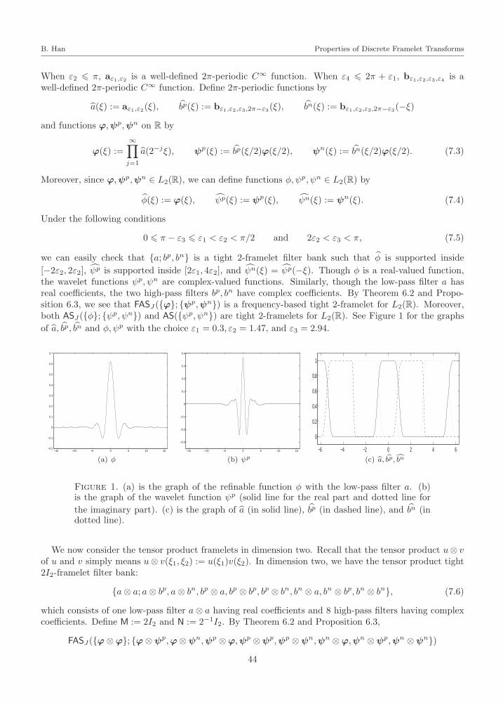
“BinHan˙mmnp” — 2013/1/13 — 11:15 — page 44 — #27i
i
i
i
i
i
i
i
B. Han Properties of Discrete Framelet Transforms
When ε2 6 π, aε1,ε2 is a well-defined 2π-periodic C∞ function. When ε4 6 2π + ε1, bε1,ε2,ε3,ε4 is awell-defined 2π-periodic C∞ function. Define 2π-periodic functions by
a(ξ) := aε1,ε2(ξ), bp(ξ) := bε1,ε2,ε3,2π−ε3(ξ), bn(ξ) := bε1,ε2,ε3,2π−ε3(−ξ)
and functions ϕ,ψp,ψn on R by
ϕ(ξ) :=
∞∏
j=1
a(2−jξ), ψp(ξ) := bp(ξ/2)ϕ(ξ/2), ψn(ξ) := bn(ξ/2)ϕ(ξ/2). (7.3)
Moreover, since ϕ,ψp,ψn ∈ L2(R), we can define functions φ, ψp, ψn ∈ L2(R) by
φ(ξ) := ϕ(ξ), ψp(ξ) := ψp(ξ), ψn(ξ) := ψn(ξ). (7.4)
Under the following conditions
0 6 π − ε3 6 ε1 < ε2 < π/2 and 2ε2 < ε3 < π, (7.5)
we can easily check that a; bp, bn is a tight 2-framelet filter bank such that φ is supported inside
[−2ε2, 2ε2], ψp is supported inside [2ε1, 4ε2], and ψn(ξ) = ψp(−ξ). Though φ is a real-valued function,the wavelet functions ψp, ψn are complex-valued functions. Similarly, though the low-pass filter a hasreal coefficients, the two high-pass filters bp, bn have complex coefficients. By Theorem 6.2 and Propo-sition 6.3, we see that FASJ(ϕ; ψ
p,ψn) is a frequency-based tight 2-framelet for L2(R). Moreover,both ASJ(φ; ψ
p, ψn) and AS(ψp, ψn) are tight 2-framelets for L2(R). See Figure 1 for the graphs
of a, bp, bn and φ, ψp with the choice ε1 = 0.3, ε2 = 1.47, and ε3 = 2.94.
−15 −10 −5 0 5 10 15−0.2
−0.1
0
0.1
0.2
0.3
0.4
0.5
0.6
0.7
(a) φ
−15 −10 −5 0 5 10 15
−0.3
−0.2
−0.1
0
0.1
0.2
0.3
0.4
(b) ψp
−6 −4 −2 0 2 4 6
0
0.2
0.4
0.6
0.8
1
(c) a, bp, bn
Figure 1. (a) is the graph of the refinable function φ with the low-pass filter a. (b)is the graph of the wavelet function ψp (solid line for the real part and dotted line for
the imaginary part). (c) is the graph of a (in solid line), bp (in dashed line), and bn (indotted line).
We now consider the tensor product framelets in dimension two. Recall that the tensor product u⊗ vof u and v simply means u⊗ v(ξ1, ξ2) := u(ξ1)v(ξ2). In dimension two, we have the tensor product tight2I2-framelet filter bank:
a⊗ a; a⊗ bp, a⊗ bn, bp ⊗ a, bp ⊗ bp, bp ⊗ bn, bn ⊗ a, bn ⊗ bp, bn ⊗ bn, (7.6)
which consists of one low-pass filter a⊗ a having real coefficients and 8 high-pass filters having complexcoefficients. Define M := 2I2 and N := 2−1I2. By Theorem 6.2 and Proposition 6.3,
FASJ (ϕ⊗ϕ; ϕ⊗ψp,ϕ⊗ψn,ψp ⊗ϕ,ψp ⊗ψp,ψp ⊗ψn,ψn ⊗ϕ,ψn ⊗ψp,ψn ⊗ψn)
44
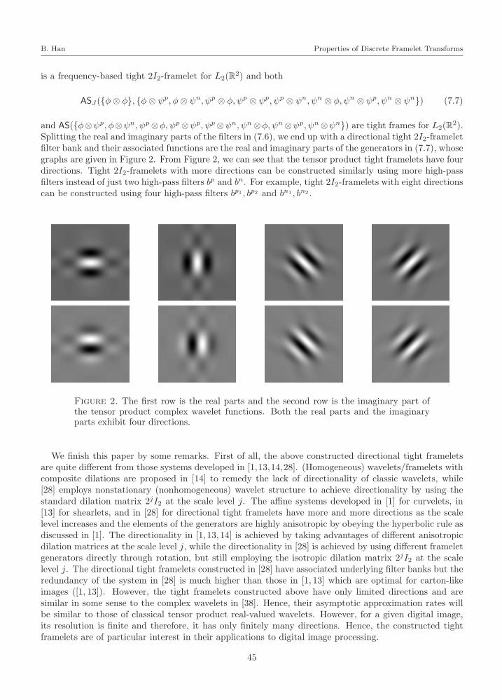
“BinHan˙mmnp” — 2013/1/13 — 11:15 — page 45 — #28i
i
i
i
i
i
i
i
B. Han Properties of Discrete Framelet Transforms
is a frequency-based tight 2I2-framelet for L2(R2) and both
ASJ(φ⊗ φ, φ⊗ ψp, φ⊗ ψn, ψp ⊗ φ, ψp ⊗ ψp, ψp ⊗ ψn, ψn ⊗ φ, ψn ⊗ ψp, ψn ⊗ ψn) (7.7)
and AS(φ⊗ψp, φ⊗ψn, ψp⊗φ, ψp⊗ψp, ψp⊗ψn, ψn⊗φ, ψn⊗ψp, ψn⊗ψn) are tight frames for L2(R2).
Splitting the real and imaginary parts of the filters in (7.6), we end up with a directional tight 2I2-frameletfilter bank and their associated functions are the real and imaginary parts of the generators in (7.7), whosegraphs are given in Figure 2. From Figure 2, we can see that the tensor product tight framelets have fourdirections. Tight 2I2-framelets with more directions can be constructed similarly using more high-passfilters instead of just two high-pass filters bp and bn. For example, tight 2I2-framelets with eight directionscan be constructed using four high-pass filters bp1 , bp2 and bn1 , bn2 .
Figure 2. The first row is the real parts and the second row is the imaginary part ofthe tensor product complex wavelet functions. Both the real parts and the imaginaryparts exhibit four directions.
We finish this paper by some remarks. First of all, the above constructed directional tight frameletsare quite different from those systems developed in [1,13,14,28]. (Homogeneous) wavelets/framelets withcomposite dilations are proposed in [14] to remedy the lack of directionality of classic wavelets, while[28] employs nonstationary (nonhomogeneous) wavelet structure to achieve directionality by using thestandard dilation matrix 2jI2 at the scale level j. The affine systems developed in [1] for curvelets, in[13] for shearlets, and in [28] for directional tight framelets have more and more directions as the scalelevel increases and the elements of the generators are highly anisotropic by obeying the hyperbolic rule asdiscussed in [1]. The directionality in [1, 13, 14] is achieved by taking advantages of different anisotropicdilation matrices at the scale level j, while the directionality in [28] is achieved by using different frameletgenerators directly through rotation, but still employing the isotropic dilation matrix 2jI2 at the scalelevel j. The directional tight framelets constructed in [28] have associated underlying filter banks but theredundancy of the system in [28] is much higher than those in [1, 13] which are optimal for carton-likeimages ([1, 13]). However, the tight framelets constructed above have only limited directions and aresimilar in some sense to the complex wavelets in [38]. Hence, their asymptotic approximation rates willbe similar to those of classical tensor product real-valued wavelets. However, for a given digital image,its resolution is finite and therefore, it has only finitely many directions. Hence, the constructed tightframelets are of particular interest in their applications to digital image processing.
45

“BinHan˙mmnp” — 2013/1/13 — 11:15 — page 46 — #29
i
i
i
i
i
i
i
i
B. Han Properties of Discrete Framelet Transforms
Acknowledgements. This research is supported in part by NSERC Canada. The author thanks Zhenpeng Zhaoat University of Alberta for plotting the graphs in Figures 1 and 2.
References
[1] E. J. Candes, D. L. Donoho. New tight frames of curvelets and optimal representations of objects with C2 singularities,Comm. Pure Appl. Math. 56 (2004), 219–266.
[2] C. K. Chui. An introduction to wavelets. Academic Press, Inc., Boston, MA, 1992.
[3] C. K. Chui, W. He. Compactly supported tight frames associated with refinable functions. Appl. Comput. Harmon.Anal. 8 (2000), 293–319.
[4] C. K. Chui, W. He, J. Stockler. Compactly supported tight and sibling frames with maximum vanishing moments, Appl.Comput. Harmon. Anal. 13 (2002), 224–262.
[5] A. Cohen, I. Daubechies. A stability criterion for biorthogonal wavelet bases and their related subband coding scheme.Duke Math. J. 68 (1992), 313–335.
[6] A. Cohen, I. Daubechies, J.-C. Feauveau. Biorthogonal bases of compactly supported wavelets. Comm. Pure Appl.Math. 45 (1992), 485–560.
[7] I. Daubechies. Orthonormal bases of compactly supported wavelets, Comm. Pure Appl. Math. 41 (1988), 909–996.
[8] I. Daubechies. Ten lectures on wavelets. SIAM, CBMS Series, 1992.
[9] I. Daubechies, B. Han. Pairs of dual wavelet frames from any two refinable functions, Constr. Approx. 20 (2004),325–352.
[10] I. Daubechies, B. Han, A. Ron, Z. Shen. Framelets: MRA-based constructions of wavelet frames. Appl. Comput.Harmon. Anal. 14 (2003), 1–46.
[11] M. Ehler. On multivariate compactly supported bi-frames, J. Fourier Anal. Appl. 13 (2007), 511–532.
[12] M. Ehler, B. Han. Wavelet bi-frames with few generators from multivariate refinable functions, Appl. Computat.Harmon. Anal. 25 (2008), 407–414.
[13] K. Guo, D. Labate. Optimally sparse multidimensional representation using shearlets. SIAM J. Math. Anal. 39 (2007),298–318.
[14] K. Guo, D. Labate, W.-Q Lim, G. Weiss, E. Wilson. Wavelets with composite dilations and their MRA properties.Appl. Comput. Harmon. Anal. 20 (2006), 202–236.
[15] B. Han. On dual wavelet tight frames. Appl. Comput. Harmon. Anal. 4 (1997), 380–413.
[16] B. Han. Approximation properties and construction of Hermite interpolants and biorthogonal multiwavelets, J. Approx.Theory. 110 (2001), 18–53.
[17] B. Han. Symmetry property and construction of wavelets with a general dilation matrix, Linear Algebra and itsApplications. 353 (2002), 207–225
[18] B. Han. Computing the smoothness exponent of a symmetric multivariate refinable function, SIAM J. Matrix Anal.Appl. 24 (2003), 693–714.
[19] B. Han. Vector cascade algorithms and refinable function vectors in Sobolev spaces, J. Approx. Theory. 124 (2003),44–88.
[20] B. Han. Compactly supported tight wavelet frames and orthonormal wavelets of exponential decay with a generaldilation matrix, J. Comput. Appl. Math. 155 (2003), 43–67.
[21] B. Han. Classification and construction of bivariate subdivision schemes, Proceedings on Curves and Surfaces Fitting:Saint-Malo 2002, A. Cohen, J.-L. Merrien, and L. L. Schumaker eds., (2003), 187–197.
[22] B. Han. Symmetric multivariate orthogonal refinable functions, Appl. Comput. Harmon. Anal.. 17 (2004), 277–292.
[23] B. Han. Matrix extension with symmetry and applications to symmetric orthonormal complex M-wavelets. J. FourierAnal. Appl. 15 (2009), 684–705.
[24] B. Han. Dual multiwavelet frames with high balancing order and compact fast frame transform. Appl. Comput. Harmon.Anal. 26 (2009), 14–42.
[25] B. Han. The structure of balanced multivariate biorthogonal multiwavelets and dual multiframelets. Math. Comp. 79(2010), 917–951.
[26] B. Han. Symmetric orthonormal complex wavelets with masks of arbitrarily high linear-phase moments and sum rules.Adv. Comput. Math. 32 (2010), 209–237.
[27] B. Han. Pairs of frequency-based nonhomogeneous dual wavelet frames in the distribution space, Appl. Comput. Har-mon. Anal. 29 (2010), 330–353.
[28] B. Han. Nonhomogeneous wavelet systems in high dimensions, Appl. Comput. Harmon. Anal. 32 (2012), 169–196.
[29] B. Han, Q. Mo. Splitting a matrix of Laurent polynomials with symmetry and its application to symmetric frameletfilter banks, SIAM J. Matrix Anal. Appl. 26 (2004), 97–124.
[30] B. Han, Q. Mo. Symmetric MRA tight wavelet frames with three generators and high vanishing moments, Appl.Comput. Harmon. Anal. 18 (2005), 67–93.
[31] B. Han, Z. Shen. Dual wavelet frames and Riesz bases in Sobolev spaces, Constr. Approx. 29 (2009), 369–406.
[32] B. Han, X. S. Zhuang. Analysis and construction of multivariate interpoalting refinable function vectors, Acta Appl.Math. 107 (2009), 143–171.
[33] R. Q. Jia. Approximation properties of multivariate wavelets, Math. Comp. 67 (1998), 647–665.
46

“BinHan˙mmnp” — 2013/1/13 — 11:15 — page 47 — #30i
i
i
i
i
i
i
i
B. Han Properties of Discrete Framelet Transforms
[34] M. J. Lai, J. Stockler. Construction of multivariate compactly supported tight wavelet frames, Appl. Comput. Harmon.Anal. 21 (2006), 324–348.
[35] S. Mallat. A wavelet tour of signal processing. Third edition. Elsevier/Academic Press, Amsterdam, 2009.
[36] Y. Meyer. Wavelets and operators. Cambridge University Press, Cambridge, 1992.
[37] A. Ron, Z. Shen. Affine systems in L2(Rd): the analysis of the analysis operator, J. Funct. Anal. 148 (1997), 408–447.
[38] I. W. Selesnick, R. G. Baraniuk, N. G. Kingsbury. The dual-tree complex wavelet transform. IEEE Signal Proc.Magazine, 123 (2005), 123–151.
[39] G. Strang, T. Nguyen. Wavelets and filter banks. Wellesley College, 2nd edition, 1996.
[40] M. Vetterli, J. Kovacevic. Wavelets and subband coding. Prentice Hall Signal Processing Series, 1995.
47