Properties of Innovations in Spot and Forward Exchange ... · 4 Properties of Innovations in Spot and Forward Exchange Rates and the Role of Money Supply Processes Hans Genberg 4.1

This PDF is a selection from an out-of-print volume from the National Bureauof Economic Research

Volume Title: Exchange Rate Theory and Practice

Volume Author/Editor: John F. O. Bilson and Richard C. Marston, eds.

Volume Publisher: University of Chicago Press

Volume ISBN: 0-226-05096-3

Volume URL: http://www.nber.org/books/bils84-1

Publication Date: 1984

Chapter Title: Properties of Innovations in Spot and Forward Exchange Ratesand the Role of Money Supply Processes

Chapter Author: Hans Genberg

Chapter URL: http://www.nber.org/chapters/c6833

Chapter pages in book: (p. 153 - 174)

4 Properties of Innovations in Spot and Forward Exchange Rates and the Role of Money Supply Processes Hans Genberg

4.1 Introduction and Summary

This paper aims to provide some new evidence concerning the determination of exchange rates by investigating relationships between innovations in spot and forward exchange rates.' In section 4.2 it is shown that under fairly general conditions this relationship depends on the properties of the stochastic processes generating the underlying determinants of exchange rates such as relative money supplies. In section 4.3 weekly data on spot and forward rates for eight countries and for five maturities are used to calculate innovations in these series which then are shown to conform to simplified versions of the model set out in section 4.2. It appears that only first-order processes generating the exogenous variables in exchange rate equations are necessary to explain the expected exchange rate dynamics contained in the data. But it is also shown that the parameters describing this first-order process tend to vary over time.

In section 4.4 the estimates, obtained from data in the foreign exchange markets, of these time-varying parameters are related to estimates of the same parameters obtained from first-order autoregressions of relative money supplies. The expected relationship between these two estimates is found

I would like to thank George Jung and Marc Vanheukelen for very efficient research assis- tance. This research was partially financed by a grant from the Fonds National Suisse de la Recherche Scientifique (grant no. 4.367-0.79.09).

1. In a previous paper written with Mario Blejer (Blejer and Genberg 1981), 1 investigated this relationship, hoping to distinguish between permanent and transitory shocks to exchange rates and to use this distinction in an explanation of deviations from purchasing power parity.

153

154 Hans Genberg

and taken as evidence that foreign exchange markets conform to at least some implications of the rational expectations hypothesis.

Section 4.5 of the paper discusses some implications of the empirical results for formulating and estimating exchange rate models, for interpreting the instability observed in estimated exchange rate equations, for explanations of the overshooting hypothesis, and for the influence of innovations in interest rate differentials on exchange rates. The last section of the paper contains some suggestions for extensions of the analysis.

4.2 A Model of Exchange Rate Determination

Suppose that the exchange rate is determined according to equation (1),* where z represents a vector of exogenous variable^,^ and u is a serially uncorrelated random variable

(1) S, = CYZ, + pEJ,+I + u,, p > 0.

With rational expectations and p < 1 this equation can be rewritten in the familiar form (2) :

(2)

Suppose furthermore that Z, is determined by (3),

(3)

where v, is another serially uncorrelated random variable. Then (2) can be transformed into

(4)

m

s, = a x pIE,Zr+l + u,. 1=0

k

z, = a0 + Calz,-[ + vt, I = I

k

Sr = n o + Cnl~r- l + n k + i v , + u,, I = I

where the k + 2 n : s are functions of a , p and the k + 1 a:$. A joint test of rationality and the models of S and Z can be achieved by estimating (3) and (4) simultaneously while taking into account the restrictions on the n : s mentioned above. Under the joint null hypothesis the estimates of the structural parameters will be more efficient than if the overidentifying restrictions were not taken into account. Extending this argument further by hypothesizing that the forward exchange rate is equal to the expected future spot rate plus a random error as in (5),4

(5) Fi+’ = EJ,,, + E:,

2. Frenkel and Mussa (1980) argue that a reduced-form equation of this type for the exchange rate can be derived from a wide variety of structural models of exchange rate determination.

3 . In the algebra which follows, for simplicity Z is assumed to contain only one element. 4. I denote by F:’’ the i-period forward exchange rate observed in period 1.

155 Spot and Forward Exchange Rates and Money Supply Processes

one can see the efficiency is improved still further by estimating jointly equations (3), (4), and (6) where the latter is derived from (2) and (3)

(6 )

k F I + I

f = 7rb + c 7rfzI-k + lT;+1 v, + E:, J = I

i = 1 , . . . ,M.

As in (4), the d : s in (6) are functions of a, p and the u:s Hence, by includ- ing the reduced-form equations for forward rates of various maturities in an estimation system containing equations for the spot rate and the Z-process, information is added, yet the number of parameters to be estimated is not increased. A strong case can thus be made for following such a procedure if the purpose of the estimation is to test the model as specified above. However, I shall argue in the next two sections that the processes determin- ing some of the Z variables, especially the money supplies, are not stable over time, implying that estimation of (3), (4), and (6) would lead to coefficients which vary with the sample period used. In order to investigate the empirical content of this assertion, 1 shall therefore proceed in a different manner by first isolating certain empirical regularities which exist in data on spot and forward rates and in particular in their innovations. I shall then relate these regularities to corresponding features of the process described in equation (3) and show that the data are consistent with the basic implication of the above analysis. That is, exchange rate movements are consistent with the rational expectations hypothesis in the sense that properties of the stochastic process generating the underlying determinants of exchange rates are appropriately reflected in spot and forward exchange rates.

From (2) and (5) I can write the current innovation in the spot rate as

Similarly, the innovation in the i-period forward rate is

IF: = Fifi - F t P l f + i = aCf3'[E,Z,+i+j - E,-IZ,+i+j] j = O

(8) ' i f 1 + €; - € , - I .

Using (3) these innovations can be written as functions of a, p, the a:$, and v,, the current forecast error of Z,. In general these functions will be fairly complicated and will allow for many types of relationships between IS and IF' for various maturities i. Substantial simplication is obtained if one re- stricts the Z-process to be of order one in either the level or the first differ- e n ~ e . ~ Thus if

(9) z, = U l . Z - 1 + v,, 5. These two cases were analyzed in Mussa (1976).

156 Hans Genberg

it follows that

i EtZ,+i - E,-lZ,+j = ulv,, i = 0 , 1, . . . ,

and that

Combining (10) and (1 I ) , we get

(12)

where qt = E: -

Similarly, if

IF: = a; IS, + q, i+ 1 I - al(E,-l + u,).

z, - z,-1 = bl(Z,- , - Z,-Z) + v,,

IF, = [p + ( 1 - p) (1 + bl + b: + . . . + bi)]

Elf! + [p + (1 - p) ( 1 + bl + . . . + bi)] + ut).

From (12) and (16) one sees that if Z follows a first-order Markov process in the levels, the innovations in forward rates tend to be smaller than the innovations in the spot rates, whereas if thejrst difference of Z follows the same process the opposite would be the case. These relationships would furthermore be more pronounced the longer is the maturity of the forward rate considered.

Rather than pursuing the theoretical analysis further, I would now like to turn to the data in order to establish that regularities exist in the relationship between IS and IF across countries, over time for a single country, and along the term structure of forward rates which are consistent with the simplified Z-processes (9) and (13) if the al parameter in these processes is allowed to vary over time.


4.3 Empirical Regularities in the Relationship Between IS and IF

vations in spot rates and forward rates as follows:6 Weekly data on spot rates and forward rates were used to calculate inno-

IFf = F f - F f f i , i = 1, 3 , 6, 9, 12,

where the time subscript spans weeks and the superscript spans months.' The sample period was April 27, 1973-August 7, 1981, and the countries included were Canada, the United Kingdom, France, Germany, Italy, the Netherlands, Switzerland, and Japan.

The analysis in the previous section suggested that innovations in forward rates are proportional to innovations in spot rates if the exogenous variable in the exchange rate equation is generated by a first-order autoregressive process in either the level or rate of change of that variable. Furthermore, the factor of proportionality should be larger than unity and increase with the length of the forecast horizon if the rate of change follows a first-order Markov process, and it should be less than one and decrease with the forecast horizon if the level is generated by this process. If the factor of proportionality did not change monotonically with the horizon the stochastic process generating the Z variable could not be of first order.

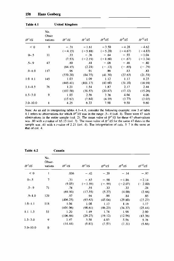
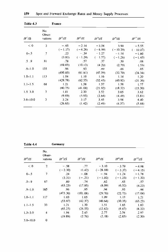
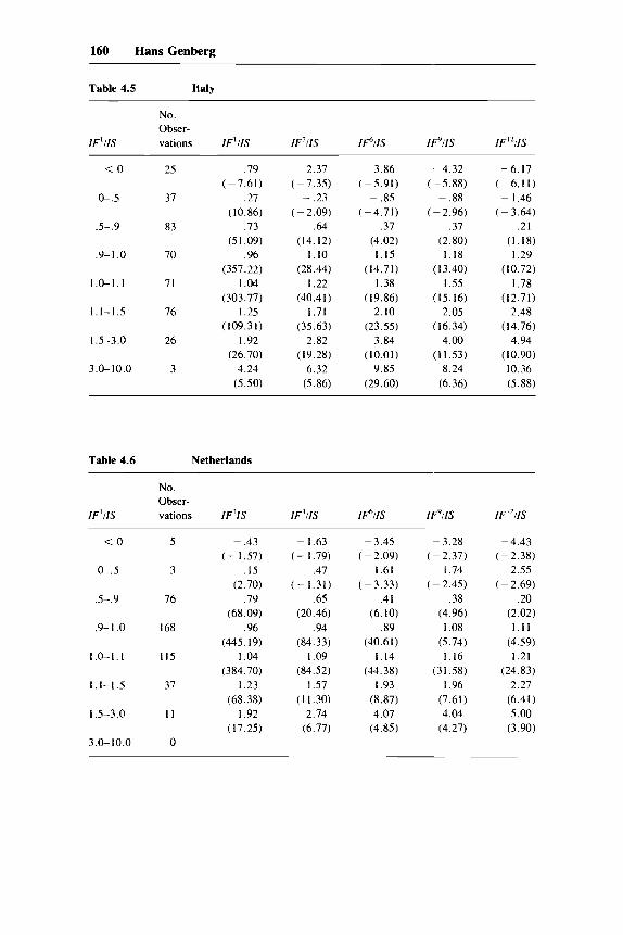
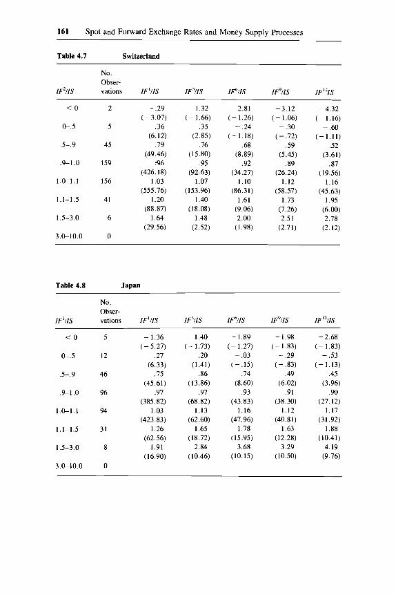
Tables 4.1-4.8 were compiled to determine whether the data contain any of the regularities suggested in the paragraph above. In the tables each row contains the mean value of IF'IIS for the observations for which IF'IIS was contained in the interval given in column 1 of that row. Column 2 gives the number of such observations. Inspection of these tables reveals that almost uniformly the data are consistent with the relationship predicted by first- order processes.8 In particular, there are only two cases out of 64 in which the factor of proportionality changes from being less than unity to being greater than unity as the forecast horizon is lengthened. An implication of this finding for the formulation of models of exchange rate determination will be discussed in section 4.5.

A second regularity apparent in these tables is that between 50% and 90% of all observations of IF'IIS lie in the interval 0.9-1.1, suggesting that shocks to exchange rates (either to the level or to the rate of change) have a high degree of persistence.' If one instead looked at the distribution of observations on IF12/IS among the same intervals as in tables 4.1-4.8, one would notice a bimodality with peaks in the (0.5, 0.9) and (1.1, 1.5) intervals reflecting the monotonicity noted above.

6. See Appendix 1 for a description of data sources and of the calculations involved. 7. In addition, the spot and forward rates (all expressed as US$/domestic currency units)

8. The main exceptions are row 4 for Italy and the Netherlands. 9. This is of course nothing but the familiar statement that exchange rates follow (approxi-

were transformed into natural logarithms before the innovations were calculated.

mately) random walks.

158 Hans Genberg

Table 4.1 United Kingdom

No. Obser-

IF‘IIS vations IF’IIS 1F”IS IF% IF911S IF1211S

< O

0-.5

.5-.9

.9-1.0

1.0-1.1

1.1-1.5

1.5-3.0

3.0-10.0

9

1 1

47

117

145

76

9

1

- .31 (-4.15)

.33 (7.53)

.80 (64.15)

.96 (370.28)

I .03 (445.41)

1.21 ( 107.58)

I .85 ( 15.67)

4.25

- 1.61 ( - 5.88) - .36

( - 2.19) .41

(2.21) .91

(84.75) 1.09

(101 .17) 1.54

(38.57) 2.56

(7.84) 6.33

- 3.50 (-5.20) - .64

( - 1.68) - .06

( - . l 3 ) .86

(41.30) 1.12

(43.68) 1.87

(20.87) 3.36

(4.19) 7.98

-4.28 (-4.67) - .93

( - .67) - .46

( - .65) .83

(27.63) 1.17

(31.18) 2. I7

(17.12) 4.04

(3.73) 9.50

-4.62 ( - 4.83) - 1.04

( - 1.34) - .80

( - .79) .83

(21.51) 1.23

(18.91) 2.44

(15.26) 4.06

(3.03) 9.60

Note: As an aid in interpreting tables 4.1-4.8, consider the following example: row 3 of table 4.1 refers to observations for which IF’IIS was in the range .5-.9 (col. I) . There were 47 such observations in the entire sample (col. 2). The mean value of IF‘IIS for these 47 observations was .80 with a t-value of 65.15 (col. 3). The mean value of IF’IIS for the same 47 dates in the sample was .41 with a r-value of 2.21 (col. 4). The interpretation of cols. 5-7 is the same as that of col. 4.

Table 4.2 Canada

No. Obser-

IF’IIS vations IF’IIS IF’IIS 1F“llS IF911S IF”I1S

< O

0-.5

.5-.9

.9-1.0

1.0-1.1

1 . 1 - I .5

1.5-3.0

3.0- 10.0

1

7

71

129

118

53

9

0

,006

.33 (9.05)

.78 (69.90)

.97 (406.25)

1.04 (401.06)

I .20 ( 106.86)

1.97 ( 14.44)

- .42

- .63 ( - 1.59)

.55 (17.55)

.94 (93.62)

I .08 (98.61)

1.49 (29.27)

3.58 (9.81)

- .39

- .98 ( - .99)

.33 (5.27)

.88 (45.04)

1.13 (46.23)

1.78 (19.12)

4.83 (7.57)

- . 14

- 1.86 ( - 2.07)

.33 (4.00)

.84 (29.88)

1.16 (34.37)

1.98 (12.56)

5.56 (7.31)

- .97

-2.14 (-2.00)

.24 (2.66)

.85 (23.27)

1.17 (25.44)

2.00 (13.36)

5.76 (5.66)


Table 4.3 France

No. Obser-

IF‘IIS vations IF’I IS IF311S IPI IS IPI IS IF”1IS

< O

0-.5

.5-.9

.9-1.0

I .o- 1 . I

I . 1-1.5

I .5-3.0

3.0-10.0

3

7

81

135

I I3

68

7

3

- .65 (-1.17)

.23 (3.83)

.78 (69.03)

.96 (450.85)

1.04 (428.78)

1.21 (90.75)

1.81 (9.69) 3.24

(26.65)

- 2. I4 (-4.26)

~ .39 ( - 1.29)

.57 (10.13)

.93 (81.81)

1.10 (82.55)

I .38 (41.08)

2.20 (3.95) 3.17 (I .42)

-3.58 ( - 6.99) - 1.27

( - 1.77) .37

(4.20) .89

(47.59) 1.16

(52.43) I .57

(21.92) 3.52

(3.64) 5.45

(2.49)

~ 3.90 ( - 10.29)

-1.14 ( - I .26)

.30 (2.79)

.88 (33.70)

1.14 (40.92)

1.58 (18.32)

3.05 (4.49) 3.98

(4.57)

-5.55 (~ 10.07) - 1.80

( - 1.43) .08

(33) .85

(24.34) I .20

(31.36) 1.77

(15.30) 3.62

(3.81) 4.40

(5.68)

Table 4.4 Germany ~

No. Obser-

IF‘IIS vations IF’I IS IF311S IF% IPIIS IFl21IS

< O

0-.5

.5-.9

.9-1 .O

1 .o- I . I

1.1-1.5

1.5-3.0

3.0- 10.0

2

7

67

185

I17

33

4

0

- .58 ( - 2.30)

.24 (3.31)

.80 (63.23)

.96 (473.30)

1.03 (53.97)

1.21 (65.23)

I .94 (19.89)

.77 (1.42) - .08

.74 (17.85)

.95 (101.08)

1.05 (42.37)

1.30 (25.55)

2.43 (2.76)

( - .21)

- 3.10 ( - 28.88)

- .94 ( - 1.02)

.62 (8.09)

.94 (29.70)

1.09 (40.64)

1.51 ( 12.62)

2.77 (2.18)

-3.79 (-3.37) -1.24

(-1.23) .65

(6.52) .95

(22.73) 1.13

(30.35) 1.65

(9.67) 2.54

(2.85)

- 4.98 (-4.15) - 1.78

( - 1.32) .57

(4.23) .94

( 17.04) 1.21

(65.23) 1.83

(8.33) 2.97

(2.30)

160 Hans Genberg

Table 4.5 Italy

No. Obser-

IF'IIS vations IF'IIS IF311S IPIIS IF'IIS IF''1IS

< O

6 . 5

.5-.9

.9-1.0

1.0-1.1

1.1-1.5

1.5-3.0

3.0-10.0

25

37

83

70

71

76

26

3

- .79 (-7.61)

.27 (10.86)

.73 (51.09)

.96 (357.22)

I .04 (303.77)

1.25 ( I 09.3 I )

I .92 (26.70)

4.24 (5.50)

- 2.37 (-7.35) - .23

( - 2.09) .64

(14.12) 1.10

(28.44) I .22

(40.4 1) 1.71

(35.63) 2.82

( 19.28) 6.32

(5.86)

-3.86 (-5.91) - .85

(-4.71) .37

(4.02) 1.15

(14.71) 1.38

( 19.86) 2.10

(23.55) 3.84

(10.01) 9.85

(29.60)

-4.32 ( - 5.88) - .88

( - 2.96) .37

(2.80) 1.18

(13.40) I .55

(15.16) 2.05

( 1 6.34) 4.00

(11.53) 8.24

(6.36)

-6.17 (-6.1 1) - 1.46

(-3.64) .21

(1.18) I .29

(10.72) 1.78

(12.71) 2.48

(14.76) 4.94

(10.90) 10.36 (5.88)

Table 4.6 Netherlands

No. Obser-

IF'IIS vations IF'IS IF'IIS IPIIS IF'IIS IF'IIIS

< O

0-.5

.5-.9

.9-1 .O

I .o- I . I

I .l-1.5

I .5-3.0

3 .O-10.0

5

3

76

168

1 I5

37

I I

0

- .43 ( - I .57)

. I5 (2.70)

.79 (68.09)

.96 (445.19)

1.04 (384.70)

I .23 (68.38)

I .92 ( 1 7.25)

- 1.63 ( - 1.79)

~ .47 (-1.31)

.65 (20.46)

.94 (84.33)

I .09 (84.52)

1.57 ( 1 I .30)

2.74 (6.77)

- 3.45 (-2.09)

~ 1.61 ( - 3.33)

.41 (6.10)

.89 (40.61)

1.14 (44.38)

I .93 (8.87) 4.07

(4.85)

- 3.28 ( - 2.37) - 1.74

( - 2.45) .38

(4.96) I .08

(5.74) 1.16

(31.58) I .96

(7.61) 4.04

(4.27)

-4.43 (-2.38)

-2.55 (-2.69)

.20 (2.02)

1 . 1 1 (4.59) 1.21

(24.83) 2.27

(6.41) 5.00

(3.90)


Table 4.7 Switzerland

No. Obser-

I F ~ I I S vations IF’IIS IF’IIS IF% IF911S IF'^

< O

cL.5

.5-.9

.9-1 .O

1 .o- I . I

1.1-1.5

1.5-3.0

3.0-10.0

2

5

45

159

156

41

6

0

- .29

.36 (6.12)

.79 (49.46)

.96 (426.18)

I .03 (555.76)

1.20 (88.87)

1.64 (29.56)

(-3.07) - 1.32

( - 1.66) .35

(2.85) .76

(1 5.80) .95

(92.63) 1.07

(153.96) 1.40

( 18.08) 1.48

(2.52)

-2.81 ( - 1.26)

( - 1.18) .68

(8.89) .92

(34.27) 1.10

(86.3 1) 1.61

(9.06) 2.00

(1.98)

- .24

-3.12 ( - 1.06) - .30

( - .72) .59

(5.45) .89

(26.24) 1.12

(58.57) 1.73

(7.26) 2.51

(2.71)

-4.32 (-1.16) - .60

( - 1.1 1) .52

(3.61) .87

(19.56) 1.16

(45.63) 1.95

(6.00) 2.78

(2.12)

Table 4.8 Japan

No. Obser-

IF’IIS vations IF’IIS IF’IIS IF% IF’IIS I F ’ ~ I I S

< O

0-.5

.5-.9

.9-1 .O

1.cL1.1

1.1-1.5

1.5-3.0

3.0-10.0

5

12

46

96

94

31

8

0

- 1.36 ( - 5.27)

.27 (6.33)

.75 (45.61)

.97 (385.82)

1.03 (423.83)

1.26 (62.56)

1.91 ( 16.90)

- 1.40 ( - 1.73)

.20 (1.41)

.86 (1 3.86)

.91 (68.82)

1.13 (62.60)

1.65 ( 18.72)

2.84 (10.46)

- 1.89 (-1.27) - .03

(-.15) .74

(8.60) .93

(43.83) 1.16

(47.96) 1.78

( 15.95) 3.68

(10.15)

- 1.98 ( - I .83) - .29

( - .83) .49

(6.02) .91

(38.30) 1.12

(40.81) 1.63

( 12.28) 3.29

(10.50)

- 2.68 ( - 1.83) - .53

(-1.13) .45

(3.96) .90

(27.12) 1.17

(31.92) 1.88

(10.41) 4.19

(9.76)

162 Hans Genberg

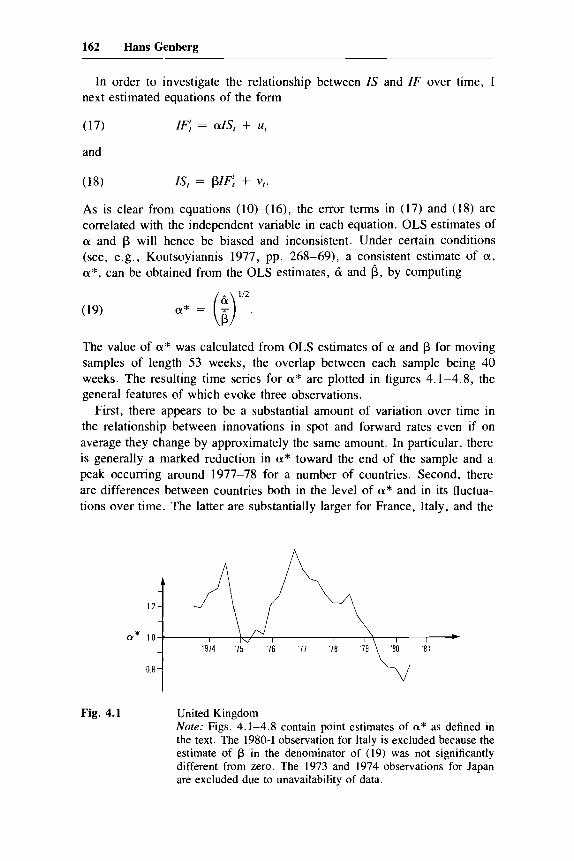
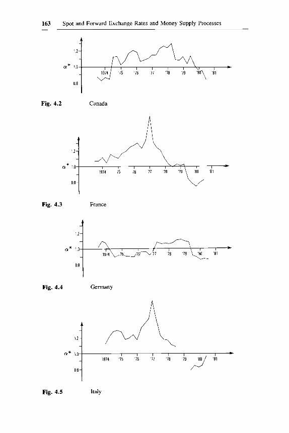
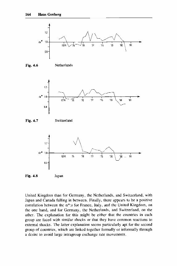
In order to investigate the relationship between IS and I F over time, 1 next estimated equations of the form

(17) IF; = alS, + u, and

IS, = pIFf + vt. As is clear from equations (lo)-( 16), the error terms in (17) and (1 8) are correlated with the independent variable in each equation. OLS estimates of a and p will hence be biased and inconsistent. Under certain conditions (see, e.g., Koutsoyiannis 1977, pp. 268-69), a consistent estimate of a , a*, can be obtained from the OLS estimates, c i and f5, by computing

The value of a* was calculated from OLS estimates of LY and p for moving samples of length 53 weeks, the overlap between each sample being 40 weeks. The resulting time series for a* are plotted in figures 4.1-4.8, the general features of which evoke three observations.

First, there appears to be a substantial amount of variation over time in the relationship between innovations in spot and forward rates even if on average they change by approximately the same amount. In particular, there is generally a marked reduction in a* toward the end of the sample and a peak occurring around 1977-78 for a number of countries. Second, there are differences between countries both in the level of a* and in its fluctua- tions over time. The latter are substantially larger for France, Italy, and the

1.2 -

a* 1.0

0.8 -

Fig. 4.1 United Kingdom Note: Figs. 4.1-4.8 contain point estimates of a* as defined in the text. The 1980-1 observation for Italy is excluded because the estimate of p in the denominator of (19) was not significantly different from zero. The 1973 and 1974 observations for Japan are excluded due to unavailability of data.


4

1.2-

a* 1.a

0.8 -

I I I I I I \I I * 1974 '75 '76 '77 '78 '79

Fig. 4.2

-

1.2- -

a* 1.0 -

0.8 -

Fig. 4.3

I I I I I I *

1974 7 5 4 1 6 - 4 7 '78 '79 '80 '81 I

Canada

France

Fig. 4.4

a*

Fig. 4.5 Italy

164 Hans Genberg

-

a* 1.0

-

0.8 -

i

I I I I I I I * ,974- '76 '77 '78 '79 '80 '81

A n n

-

1.2- -

a* 1 0

-

08-

Fig. 4.6 Netherlands

I I I - 1 I I I I * 1974 '75 '76 '77 '78 '79 ' 8 0 - ' 8 1

Fig. 4.7 Switzerland

Fig. 4.8 Japan

United Kingdom than for Germany, the Netherlands, and Switzerland, with Japan and Canada falling in between. Finally, there appears to be a positive correlation between the ci*:s for France, Italy, and the United Kingdom, on the one hand, and for Germany, the Netherlands, and Switzerland, on the other. The explanation for this might be either that the countries in each group are faced with similar shocks or that they have common reactions to external shocks. The latter explanation seems particularly apt for the second group of countries, which are linked together formally or informally through a desire to avoid large intragroup exchange rate movements.


In the next section the variability over time and across countries noted in these figures will be related to variations in monetary policy. Some implications of the other empirical regularities in the relationship between IF and IS noted above will be taken up in the next section of the paper.

4.4 The Role of Differences in Monetary Policy

Two views may be taken of the differences over time in the responses of the spot and forward exchange rates to common shocks. One is that the differences are due to changes over time in the stochastic processes govem- ing the underlying determinants of the exchange rate. Such changes might occur because of changes in monetary policy regimes from, say, a strategy of preannounced growth rates to a feedback rule for the money supply. Changes in the money supply process might also result from changes over time in the degree of intervention in the foreign exchange market." Another view is that the differences over time and across countries we observe in figures 4.1-4.8 are due to changes over time in the sources of the shocks (monetary versus real shocks, for example), and that the stochastic properties governing each type of shock are invariant with respect to time.

In what follows I shall investigate the implications of the first of these views, concentrating exclusively on monetary policy by assuming that the money supply of each country relative to the money supply in the United States is an important determinant of that country's exchange rate. I shall then hypothesize that (the natural logarithm of) the ratio of money supplies, mi,,, follows a first-order autoregressive process with an autoregressive parameter which varies over time." Hence,

(20) mi,, = ai.0 + ai,I,rmi,t-1 + ui,r.

According to equation (12) of section 4.2, the autoregressive parameter a l obtained from (20) should be related to the factor of proportionality between innovations in forward and spot exchange rates under the joint hypothesis described by ( l ) , Z, = m,, ( 5 ) , (20), and rational expectations. In order to investigate this hypothesis, I first estimated (20) for each of the countries in the sample, using monthly money supply data from January 1972 to May 198 1. The al parameter was estimated for 36-month-long moving samples with the overlap between adjacent samples being 24 months. The resulting point estimates were then correlated with the estimate of a obtained from (19), both over time and across countries.I2 Under the null hypothesis these

10. These examples were chosen because I believe that they have been important in a number of countries in recent years.

I I , In fact m,,, = In (w/M:) where Mu> is the money supply for the United States and M' is the money supply for country i. See Appendix 1 for data sources.

12. For point estimates, see table 4.A.1. For the resulting coefficients, see table 4.A.2. In this part of the paper, I worked only with estimates of a obtained with innovations in 12-month forward rates.

166 HansGenberg

09 I 01974

‘81 a,

r=O 57 0

‘77

0.8 0.9 1.0 1 1 1 2 1 3 a

Fig. 4.9 Averages of eight countries

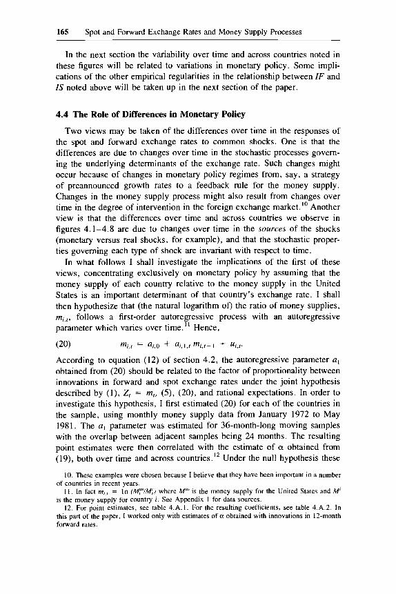
correlations should be positive. Figures 4.9 and 4.10 contain scatter dia- grams of the estimates of the autoregressive parameter obtained from (19) and (20) for cross-country and time series sample averages. The correlation coefficient between the two variables (denoted r in the figures) is in both cases significantly larger than zero at the 90% level. On this criterion, there-

GI

a, 0 7 -

06-

08 0 9 1 0 1 1 1 2 1 3 a

Fig. 4.10 Averages of 8 years


fore, the null hypothesis is not rejected by the data and one may conclude that when agents form expectations about future spot rates the properties of the stochastic process generating the money supply are indeed taken into account in a manner consistent with the rational expectations hypothesis.

Confirmation of this assertion is obtained if first-order autoregressive parameters are estimated for the logarithms of the own-country money supplies (i.e., not relative to the United States) and the resulting point estimates are correlated (across countries) with the coefficient obtained from (19). The correlation coefficient here is .68, significantly larger than zero at the 95% level. If individual countries are examined one finds that the data from the United Kingdom, France, Italy, and Japan corroborate the null hypothesis; that the evidence from Canada is mixed; and that Germany, the Netherlands, and Switzerland fail to corroborate the hypothesis. Similar ambiguities appear when cross-country correlations are calculated for each of the 8 years. Given the exclusion of all variables which affect exchange rates except money supplies, and especially given the problems of dating exactly changes in the autoregressive parameter in the two ways suggested here, it is proba- bly too much to hope that each country and each year should conform to the predictions of the theory. Hence 1 view the average data as more appropriate for examining the null hypothesis as posed here, and I retain the conclusion that changes in monetary policy strategies which manifest themselves as changes in the money supply processes are taken into account by agents in forming expectations. I now turn to some implications of this conclusion, and of those of the previous section, for the appropriate conduct of empirical estimation of exchange rate equations, for interpretation of existing empirical work, and for judging the empirical validity of alternative theoretical models of exchange rate determination.

4.5 Implications

The theoretical framework for exchange rate determination set out in section 4.2 incorporating the rational expectations hypothesis implied that the relationship between innovations in spot rates, IS , and innovations in forward rates, IF, should depend, inter alia, on the stochastic process generating the underlying determinants of exchange rates. In the previous section it was shown that part of the differences in the ratio of IF to IS observed in data over time and between countries can indeed be explained by differences over time and between countries in the processes generating relative money supplies as suggested by the theory. In section 4.3 it was also shown that the size of the ratio of innovations in forward rates to innovations in spot rates depends on the maturity of the forward rate involved. This dependence was shown to be monotonic in the sense that the ratio increased (decreased) steadily with the maturity of the forward rate if the ratio for the 1-month forward rate was greater (less) than unity. Oscillations around unity were

168 Hans Genberg

extremely rare. Some implications of these and other empirical findings will now be taken up.

4.5.1 Formulating and Estimating Exchange Rate Equations

In section 4.2, it was shown that if agents form expectations partly on the basis of their estimate of the process generating the exogenous variables, increased efficiency can be obtained in estimation of exchange rate equations if the latter are estimated jointly with the process for the exogenous variable and if the appropriate cross-equation restrictions are taken into account. The evidence presented here implies that this gain in efficiency will be achieved in practice since agents do seem to rely on information contained in the money supply processes. The results also imply that further gains in efficiency will be obtained if equations for forward exchange rates of different maturities are included in the joint estimation because these forward rates will be determined as spot rates are, and the processes generating the exogenous variables will have an identifiable impact on them as well.

The results of the previous section suggest, however, that in implement- ing the joint estimation mentioned above it is necessary to allow for changes over time in the process generating the exogenous variables, at least as far as the money supply is concerned. This increases the complexity of the procedure, but it is essential if problems of parameter instability are to be avoided.

4.5.2 Instability of Coefficients in Empirical Exchange Rate Equations

It has been argued that explanations of exchange rate movements based on movements in money supplies are inadequate because, among other reasons, estimated exchange rate equations which restrict themselves to using current and lagged money supplies as regressors appear to be unstable in the sense that the coefficients on the money supply terms vary with the sample period (see, e.g., Hodrick 1979; Dombusch, 1980). An implication of the results presented here is that such instability is not necessarily a result of an inadequacy of the monetary model, but rather a consequence of inappro- priate implementation of that model. If the processes generating money supplies change over time, then the model presented in section 4.2 implies that the coefficients relating the current spot rate to current and lagged money supplies should change. Hence observed instability may simply be a reflec- tion of instability of monetary policy rather than inadequacy of any particular theoretical framework. l 3

13. This is of course not to suggest that only money supply processes matter. Coefficient instability will appear whenever the process generating the exogenous variable, whatever it may be, changes.


4.5.3 Overshooting

The concept of overshooting has become a popular one in the discussion of exchange rate movements and exchange rate policy. The most common reasons given for the emergence of overshooting are some forms of stickiness somewhere in the economic system which prevent prices and quantities from adjusting rapidly. In the framework presented here overshooting may be related to the relative size of IS or IF. If IS is larger than IF then we might say that the spot rate is overshooting in the sense that the current spot rate moves by more than does the expected future spot rate. Concerning the reason for such movements, the present paper has emphasized an alternative to the stickiness explanation which is the role of the processes generating underlying determinants of exchange rates in general and money supplies in particular. As noted above, if the levels of money supplies follow first-order autoregressive processes, one should expect to observe overshooting as defined here. On the other hand, if the rates of change of money supplies follow first-order autoregressive processes, then one should expect to observe undershooting. In tables 4.1-4.8 it appears that, far from being a dominant feature of the recent period of flexible rates, overshooting is no more common than undershooting for the countries examined here.

4.5.4 The Role of “News”

Frenkel (198 1) implemented the idea that unexpected movements in exchange rates should be related only to unexpected movements in their determinants by using as a regressor in an exchange rate equation the innovation in the interest rate differential between the countries in question. Letting i f stand for this interest differential and assuming that uncovered interest parity holds, we have i, = E&+, - S,, which can be rewritten as

(21)

or

(22)

Equation (22) shows that the innovation in the interest differential is equal to the difference between the innovations in the forward rate and the spot rate. Letting ZFIIS = (Y, it then follows that if one runs a regression of innovations in the spot exchange rate on innovations in the interest differential, then one should expect to find a positive, negative, or zero slope coefficient according to whether (Y is larger, smaller, or equal to one. Fren- kel’s sample included France, Germany, and the United Kingdom for the period June 1973-July 1979. Looking at figures 4.1, 4.3, and 4.4, it appears that a was systematically greater than unity for France and the United King- dom but was both smaller and greater than unity for Germany during this

if = (&&+I - E f - J t + d - (S, - E,- lS , ) + E,-IS,+~

- E f - I S ,

if = IF, - IS, - E f - l i f .

170 Hans Genberg

sample period. On the argument presented here, the two former countries should yield significantly positive coefficients in Frenkel’s regressions, whereas for Germany one would expect a coefficient not significantly different from zero. An examination of Frenkel’s results shows this to be the case, thus providing an additional bit of evidence in favor of the interpretation of the relationship between IS and IF suggested in this paper.

4.5.5 Structure of Theoretical Models of Exchange Rate Determination

The relationship between IS and IF depends in theory on both the structure of the economy and the processes generating the exogenous variables in the exchange rate equations. Under some simplifying assumptions noted in section 4.2, it was shown that this relationship varies monotonically with the maturity of the forward rate. In section 4.3 it was found that the data contain almost exclusively such monotonic relationships. This finding implies that, whatever economic model one chooses to work with, it need not result in more complicated exchange rate dynamics than those generated by a first-order difference equation in order to be compatible with the data. Models which generate more complicated adjustment patterns, such as overshooting followed by undershooting (as defined in the previous subsection), may be theoretically interesting, but they do not appear to warrant serious empirical consideration because the data simply do not contain such adjustment patterns.

In the same vein, in order to construct models to allow for the possibility of overshooting, it is not necessary to rely on slow adjustment and various degrees of sticky prices. Overshooting may simply be a result of the properties of the money supply process responsible for movements in the exchange rate. This explanation ought to be given more attention, especially in discussions of the policy implications of the overshooting hypothesis.

4.6 Extensions

The present paper has presented a bit of new evidence consistent with the rational expectations hypothesis as applied to exchange rate behavior. As already noted, further tests of this hypothesis and more efficient estimations of exchange rate equations can be obtained by following the methods suggested in sections 4.2 and 4.5.1. The main difficulty of implementation would seem to stem from the hypothesized time dependence of the coefficients in the money supply equations. The procedure followed in this paper represents a first rough attempt to deal with this problem. More detailed treatment would seem to be an area of potentially significant payoff. Two different paths may be followed. One is to attempt to model the time dependence directly in terms of the presumably shifting objectives of the monetary policy authorities. This would involve attempts to model changes in the strategy of the central bank and would be subject to all the usual difficulties encountered in trying to estimate policy reaction functions.

171 S p o t and Forward Exchange Rates and Money Supply Processes

Another possible path to follow would be to assume that agents view the money supply (and other variables) as being generated by a combination of temporary and permanent shocks and then to use results from signal extrac- tion analysis to describe the nature of the current shocks. Kalman filtering techniques offer a possible tool for this line of inquiry.

Appendix 1: Data

The data on exchange rates were those published by the Harris Bank. Weekly spot rates and 30-, 60-, 90-, 180-, and 360-day forward rates were available for all eight countries. In addition, 270-day forward rates were available for the United Kingdom and Canada. To calculate innovations in forward rates for 90, 180, 270, and 360 days, forward rates of 120, 210, 300, and 390 days were necessary. These were obtained by interpolation using the forward rate with the closest matching maturity. Money supply data were taken from the International Monetary Fund’s International Fi- nancial Statistics data tape. The M I (line 34 of International Financial Sta- tistics) definition of money was used. For the United States it was necessary to supplement the data from the tape with data from the Federal Reserve Bulletin starting in 1979. The money supply data were seasonally adjusted prior to the estimation of the autoregressive processes.

Appendix 2: Calculation of Estimates of cx and al over Time

Given the overlapping sample periods used to estimate the first-order autoregressive process for the ratio of the money supplies, it is possible to justify calculating the a , coefficient appropriate for any given year in a number of ways. Only one method was explored here. This took the following form:

Let a I ,, be the estimated first-order autoregressive parameter in equation (20) for the sample period ending with December of year t . Then the parameter for year t , d , ,,, used in the correlation analysis was calculated according to

= + 2 ~ 1 , , + 1 + aI,,+2)/4, t = 1974, . . . 7 1979;

t = 1980;

t = 1981.

d,., = + 2al. ,+lY3,

A I J = bl,,?

The resulting parameters are contained in table 4.A. 1.

Table 4.A.1 Estimates of First-Order Autoregressive Parameter in Relative Money Supply Series

United Kingdom Canada France Germany Italy Netherlands Switzerland Japan

1974 1975 1976 1977 1978 1979 1980 1981

.87

.98

.97

.97

.92

.74

.55

.43

.86

.77

.56

.47

.53

.54

.49

.45

.94

.91

.85

.83

.88

.85

.78

.74

.94

.89

.79

.79

.74

.65

.69

.77

.94

.96

.99 1.01 1.01 .98 .94 .92

.90

.93

.84

. I9

.74

.64

.51

.54

.83

.63

.65

.78

.84

.90

.96

.99

-

.89

.83

.76

.71

.68

.67

.69

Table 4.A.2 Estimates of the Parameter a (cf. Equation [19]) ~~

United Kingdom Canada France Germany Italy Netherlands Switzerland Japan

1.29 .87 1.12 1.08 1.13 1.12 1.09 - 1974 1975 1 .oo 1.03 1.11 .93 1.28 .95 .97 1.26 1976 1.21 1.20 1.27 .98 1.19 1.10 1.15 1.04 1977 1.45 1.16 1.66 .99 1.68 1.18 1.16 1.10 1978 1.22 1.25 1.09 1.06 1.18 1.02 I .04 1.03 1979 1.08 1.14 1.01 1.10 I .32 1.11 1.10 1.06 1980 .80 .96 .75 .87 .84 1.06 .82 .93 1981 .83 .85 .83 .87 .97 .80 .85 .93

174 Hans Genberg

For the calculation of the parameter (Y (cf. eq. [ 191 in section 4.3) corresponding to a given year t , the estimate a: ( as defined in the equation following [ 191 in the main text) corresponding to the sample ending with the last week of year t was used. The resulting parameters are contained in table 4.A.2.

References

Blejer, Mario, and Genberg, Hans. 1981. Permanent and transitory shocks to exchange rates: Measurement and implications for purchasing power panty. Manuscript.

Dornbusch, Rudiger. 1980. Exchange rate economics: Where do we stand? Brookings Papers on Economic Activity, no. 2, pp. 143-85.

Frenkel, Jacob. 1981. Flexible exchange rates, prices and the role of “news”: Lessons from the 1970s. Journal of Political Economy 89:665- 705.

Frenkel, Jacob, and Mussa, Michael. 1980. The efficiency of foreign exchange markets and measures of turbulence. American Economic Review

Hodrick, Robert. 1979. On the monetary analysis of exchange rates, a com- ment. In Policies for employment, prices, and exchange rates, ed. Karl Brunner and Allan H. Meltzer. Carnegie-Rochester Conference Series on Public Policy no. 1 1 . Amsterdam: North-Holland.

70:374-8 1.

Koutsoyiannis, A. 1977. Theory of econometrics. London: Macmillan. Mussa, Michael. 1976. The exchange rate, the balance of payments, and

monetary and fiscal policy under a regime of controlled floating. Scandi- navian Journal of Economics 78:229-48.

Documents

Properties of Innovations in Spot and Forward Exchange ... · 4 Properties of Innovations in Spot and Forward Exchange Rates and the Role of Money Supply Processes Hans Genberg 4.1