Properties of range-based volatility estimators

Peter Molnar1

Abstract

Volatility is not directly observable and must be estimated. Estimator based ondaily close data is imprecise. Range-based volatility estimators provide signifi-cantly more precision, but still remain noisy volatility estimates, something thatis sometimes forgotten when these estimators are used in further calculations.

First, we analyze properties of these estimators and find that the best esti-mator is the Garman-Klass (1980) estimator. Second, we correct some mistakesin existing literature. Third, the use of the Garman-Klass estimator allows us toobtain an interesting result: returns normalized by their standard deviations areapproximately normally distributed. This result, which is in line with resultsobtained from high frequency data, but has never previously been recognized inlow frequency (daily) data, is important for building simpler and more precisevolatility models.Key words: volatility, high, low, rangeJEL Classification: C58, G17, G32

1. Introduction

Asset volatility, a measure of risk, plays a crucial role in many areas offinance and economics. Therefore, volatility modelling and forecasting becomeone of the most developed parts of financial econometrics. However, since thevolatility is not directly observable, the first problem which must be dealt withbefore modelling or forecasting is always a volatility measurement (or, moreprecisely, estimation).

Consider stock price over several days. From a statistician’s point of view,daily relative changes of stock price (stock returns) are almost random. More-over, even though daily stock returns are typically of a magnitude of 1% or2%, they are approximately equally often positive and negative, making aver-age daily return very close to zero. The most natural measure for huw muchstock price changes is the variance of the stock returns. Variance can be easilycalculated and it is a natural measure of the volatility. However, this way we

1I would like to thank to Jonas Andersson, Milan Basta, Ove Rein Hetland, Lukas Laffers,Michal Zdenek and anonymous referees for helpful comments. Norwegian School of Economics,Department of Finance and Management Science, Helleveien 30, 5045 Bergen, Norway andNorwegian University of Science and Technology, Department of Industrial Economics andTechnology Management, 7491 Trondheim, Norway, email: Peter.Molnar@iot.ntnu.no

Preprint submitted to Elsevier June 8, 2011

can get only an average volatility over an investigated time period. This mightnot be sufficient, because volatility changes from one day to another. Whenwe have daily closing prices and we need to estimate volatility on a daily basis,the only estimate we have is squared (demeaned) daily return. This estimateis very noisy, but since it is very often the only one we have, it is commonlyused. In fact, we can look at most of the volatility models (e.g. GARCH classof models or stochastic volatility models) in such a way that daily volatility isfirst estimated as squared returns and consequently processed by applying timeseries techniques.

When not only daily closing prices, but intraday high frequency data areavailable too, we can estimate daily volatility more precisely. However, highfrequency data are in many cases not available at all or available only overa shorter time horizon and costly to obtain and work with. Moreover, due tomarket microstructure effects the volatility estimation from high frequency datais rather a complex issue (see Dacorogna et al. 2001).

However, closing prices are not the only easily available daily data. For themost of financial assets, daily open, high and low prices are available too. Range,the difference between high and low prices is a natural candidate for the volatilityestimation. The assumption that the stock return follows a Brownian motionwith zero drift during the day allows Parkinson (1980) to formalize this intuitionand derive a volatility estimator for the diffusion parameter of the Brownianmotion. This estimator based on the range (the difference between high andlow prices) is much less noisy than squared returns. Garman and Klass (1980)subsequently introduce estimator based on open, high, low and close prices,which is even less noisy. Even though these estimators have existed for morethan 30 years, they have been rarely used in the past by both academics andpractitioners. However, recently the literature using the range-based volatilityestimators started to grow (e.g. Alizadeh, Brandt and Diebold (2002), Brandtand Diebold (2006), Brandt and Jones (2006), Chou (2005), Chou (2006), Chou,Liu (2010)). For an overview see Chou and Liu (2010).

Despite increased interest in the range-based estimators, their properties aresometimes somewhat imprecisely understood. One particular problem is thatdespite the increased accuracy of these estimators in comparison to squared re-turns, these estimators still only provide a noisy estimate of volatility. However,in some manipulations (e.g. division) people treat these estimators as if theywere exact values of the volatility. This can in turns lead to flawed conclusions,as we show later in the paper. Therefore we study these properties.

Our contributions are the following. First, when the underlying assumptionsof the range-based estimators hold, all of them are unbiased. However, takingthe square root of these estimators leads to biased estimators of standard de-viation. We study this bias. Second, for a given true variance, distribution ofthe estimated variance depends on the particular estimator. We study thesedistributions. Third, we show how the range-based volatility estimators shouldbe modified in the presence of opening jumps (stock price at the beginning ofthe day typically differs from the closing stock price from the previous day).

Fourth, the property we focus on is the distribution of returns standardized

2

by standard deviations. A question of interest is how this is affected when thestandard deviations are estimated from range-based volatility estimators. Thequestion whether the returns divided by their standard deviations are normallydistributed has important implications for many fields in finance. Normality ofreturns standardized by their standard deviations holds promise for simple-to-implement and yet precise models in financial risk management. Using volatilityestimated from high frequency data, Andersen, Bollerslev, Diebold and Labys(2000), Andersen, Bollerslev, Diebold, Ebens (2001), Forsberg and Bollerslev(2002) and Thamakos and Wang (2003) show that standardized returns are in-deed Gaussian. Contrary, returns scaled by standard deviations estimated fromGARCH type of models (which are based on daily returns) are not Gaussian,they have heavy tails. This well-known fact is the reason why heavy-taileddistributions (e.g. t-distribution) were introduced into the GARCH models.We show that when properly used, range-based volatility estimators are preciseenough to replicate basically the same results as those of Andersen et al. (2001)obtained from high frequency data. To our best knowledge, this has not beenpreviously recognized in the daily data. Therefore volatility models built uponhigh and low data might provide accuracy similar to models based upon highfrequency data and still keep the benefits of the models based on low frequencydata (much smaller data requirements and simplicity).

The rest of the paper is organized in the following way. In Section 2, wedescribe existing range-based volatility estimators. In Section 3, we analyzeproperties of range-based volatility estimators, mention some caveats relatedto them and correct some mistakes in the existing literature. In Section 4we empirically study the distribution of returns normalized by their standarddeviations (estimated from range-based volatility estimators) on 30 stock, thecomponents of the Dow Jones Industrial Average. Section 5 concludes.

2. Overview

Assume that price P follows a geometric Brownian motion such that log-price p = ln(P ) follows a Brownian motion with zero drift and diffusion σ.

dpt = σdBt (1)

Diffusion parameter σ is assumed to be constant during one particular day, butcan change from one day to another. We use one day as a unit of time. Thisnormalization means that the diffusion parameter in (1) coincides with the dailystandard deviation of returns and we do not need to distinguish between thesetwo quantities. Denote the price at the beginning of the day (i.e. at the timet = 0) O (open), the price in the end of the day (i.e. at the time t = 1) C(close), the highest price of the day H, and the lowest price of the day L. Thenwe can calculate open-to-close, open-to-high and open-to-low returns as

c = ln(C)− ln(O) (2)

h = ln(H)− ln(O) (3)

3

l = ln(L)− ln(O) (4)

Daily return c is obviously a random variable drawn from a normal distributionwith zero mean and variance (volatility) σ2

c ∼ N(0, σ2) (5)

Our goal is to estimate (unobservable) volatility σ2 from observed variables c,h and l. Since we know that c2 is an unbiased estimator of σ2,

E(c2)

= σ2 (6)

we have the first volatility estimator (subscript s stands for ”simple”)

σ2s = c2 (7)

Since this simple estimator is very noisy, it is desirable to have a better one. Itis intuitively clear that the difference between high and low prices tells us muchmore about volatility than close price. High and low prices provide additionalinformation about volatility. The distribution of the range d ≡ h − l (thedifference between the highest and the lowest value) of Brownian motion isknown (Feller (1951)). Define P (x) to be the probability that d ≤ x during theday. Then

P (x) =

∞∑n=1

(−1)n+1

n

{Erfc

((n+ 1)x√

2σ

)− 2Erfc

(nx√2σ

)+ Erfc

((n− 1)x√

2σ

)}(8)

whereErfc(x) = 1− Erf(x) (9)

and Erf(x) is the error function. Using this distribution Parkinson (1980)calculates (for p ≥ 1)

E (dp) =4√π

Γ

(p+ 1

2

)(1− 4

2p

)ζ (p− 1)

(2σ2)

(10)

where Γ (x) is the gamma function and ζ (x) is the Riemann zeta function.Particularly for p = 1

E (d) =√

8πσ (11)

and for p = 2E(d2)

= 4 ln (2)σ2 (12)

Based on formula (12), he proposes a new volatility estimator:

σ2P =

(h− l)2

4 ln 2(13)

Garman and Klass (1980) realize that this estimator is based solely on quan-tity h−l and therefore an estimator which utilizes all the available information c,

4

h and l will be necessarily more precise. Since search for the minimum varianceestimator based on c, h and l is an infinite dimensional problem, they restrictthis problem to analytica estimators, i.e. estimators which can be expressedas an analytical function of c, h and l. They find that the minimum varianceanalytical estimator is given by the formula

σ2GKprecise = 0.511 (h− l)2 − 0.019 (c(h+ l)− 2hl)− 0.383c2 (14)

The second term (cross-products) is very small and therefore they recommendneglecting it and using more practical estimator:

σ2GK = 0.5 (h− l)2 − (2 ln 2− 1) c2 (15)

We follow their advice and further on when we talk about Garman-Klass volatil-ity estimator (GK), we refer to (15). This estimator has additional advantageover (14) - it can be simply explained as an optimal (smallest variance) combi-nation of simple and Parkinson volatility estimator.

Meilijson (2009) derives another estimator, outside the class of analyticalestimators, which has even smaller variance than GK. This estimator is con-structed as follows.

σ2M = 0.274σ2

1 + 0.16σ2s + 0.365σ2

3 + 0.2σ24 (16)

whereσ21 = 2

[(h′ − c′)2 + l′

](17)

σ23 = 2 (h′ − c′ − l′) c′ (18)

σ24 = − (h′ − c′) l′

2 ln 2− 5/4(19)

where c′ = c, h′ = h, l′ = l if c > 0 and c′ = −c, h′ = −l, l′ = −h if c < 0.2

Rogers and Satchell (1991) derive an estimator which allows for arbitrarydrift.

σ2RS = h(h− c) + l(l − c) (20)

There are two other estimators which we should mention. Kunitomo (1992)derives a drift-independent estimator, which is more precise than all the pre-viously mentioned estimators. However ”high” and ”low” prices used in hisestimator are not the highest and lowest price of the day. The ”high” and ”low”used in this estimator are the highest and the lowest price relative to the trendline given by open and high prices. These ”high and ”low” prices are unknownunless we have tick-by-tick data and therefore the use of this estimator is verylimited.

2This estimator is not analytical, because it uses different formula for days when c > 0than for days when c < 0.

5

Yang and Zhang (2000) derive another drift-independent estimator. How-ever, their estimator can be used only for estimation of average volatility overmultiple days and therefore we do not study it in our paper.

Efficiency of a volatility estimator σ2 is defined as

Eff(σ2) ≡var

(σ2s

)var

(σ2) (21)

Simple volatility estimator has by definition efficiency 1, Parkinson volatility es-timator has efficiency 4.9, Garman-Klass 7.4 and Meilijson 7.7. Rogers, Satchellhas efficiency 6.0 for the zero drift and larger than 2 for any drift.

Remember that all of the studied estimators except for Rogers, Satchell arederived under the assumption of zero drift. However, for most of the financialassets, mean daily return is much smaller than its standard deviation and cantherefore be neglected. Obviously, this is not true for longer time horizons (e.g.when we use yearly data), but this is a very good approximation for daily datain basically any practical application.

Further assumptions behind these estimators are continuous sampling, nobid-ask spread and constant volatility. If prices are observed only infrequently,then the observed high will be below the true high and observed low will be abovethe true low, as was recognized already by Garman and Klass (1980). Bid-askspread has the opposite effect: observed high price is likely to happen at ask,observed low price is likely to happen at the low price and therefore the differencebetween high and low contains in addition bid-ask spread. These effects work inthe opposite direction and therefore they will at least partially cancel out. Moreimportantly, for liquid stocks both these effects are very small. In this paper wemaintain the assumption of constant volatility within the day. This approachis common even in stochastic volatility literature (e.g. Alizadeh, Brandt andDiebold 2002) and assessing the effect of departing from this assumption isbeyond the scope of this paper. However, this is an interesting avenue forfurther research.

3. Properties of range-based volatility estimators

The previous section provided an overview of range-based volatility estima-tors including their efficiency. Here we study their other properties. Our mainfocus is not their empirical performance, as this question has been studied before(e.g. Bali and Weinbaum (2005)). We study the performance of these estima-tors when all the assumptions of these estimators hold perfectly. This is moreimportant than it seems to be, because this allows us to distinguish between thecase when these estimators do not work (assumptions behind them do not hold)and the case when these estimators work, but we are misinterpreting the results.This point can be illustrated in the following example. Imagine that we want tostudy the distribution of returns standardized by their standard deviations. Weestimate these standard deviations as a square root of the Parkinson volatility

6

estimator (13) and find that standardized returns are not normally distributed.Should we conclude that true standardized returns are not normally distributedor should we conclude that the Parkinson volatility estimator is not appropriatefor this purpose? We answer this and other related questions.

To do so, we ran 500000 simulations, one simulation representing one tradingday. During every trading day log-price p follows a Brownian motion with zerodrift and daily diffusion σ = 1. We approximate continuous Brownian motionby n = 100000 discrete intraday returns, each drawn from N(0, 1/

√n).3 We

save high, low and close log-prices h, l, c for every trading day4.

3.1. Bias in σ

All the previously mentioned estimators are unbiased estimators of σ2. There-fore, square root of any of these estimators will be a biased estimator of σ. Thisis direct consequence of well known fact that for a random variable x the quan-tities E(x2) and E(x)2 are generally different. However, as I document later,

using√σ2 as σ, as an estimator of σ, is not uncommon. Moreover, in many

cases the objects of our interests are standard deviations, not variances. There-

fore, it is important to understand the size of the error introduced by using√σ2

instead of σ and potentially correct for this bias. Size of this bias depends onthe particular estimator.

As can be easily proved, an unbiased estimator σs of the standard deviation

σ based on

√σ2s is

σs =

√σ2s ×

√π

2= |c| ×

√π/2 (22)

Using the results (11) and (13) we can easily find that an estimator of standarddeviation based on range is

σP =h− l

2×√π

2=

√σ2P ×

√π ln 2

2(23)

Similarly, when we want to evaluate the bias introduced by using√σ2 instead

of σ for the rest of volatility estimators, we want to find constants cGK , cM andcRS such that

σGK =

√σ2GK × cGK (24)

3Such a high n allows us to have almost perfectly continuous Brownian motion and havingso many trading days allow us to know the distributions of range based volatility estimatorswith very high precision. Simulating these data took one months on an ordinary computer(Intel Core 2 Duo P8600 2.4 GHz, 2 GB RAM).

Note that we do not derive analytical formulas for the distributions of range-based volatilityestimators. Since these formulas would not bring additional insights into the questions westudy, their derivation is behind the scope of this paper.

4Open log-price is normalized to zero.

7

σM =

√σ2M × cM (25)

σRS =

√σ2RS × cRS (26)

From simulated high, low and close log-prices h, l, c we estimate volatilityaccording to (7), (13), (15), (16), (20) and calculate mean of the square rootof these volatility estimates. We find that cs = 1.253, cP = 1.043 (what is inaccordance with theoretical values

√π/2 = 1.253 and

√π ln 2/2 = 1.043) and

cGK = 1.034, cM = 1.033 and cRS = 1.043. We see that the square root of thesimple volatility estimator is a severely biased estimator of standard deviation(bias is 25%), whereas bias in the square root of range-based volatility estimatorsis rather small (3% - 4%).

Even though it seems obvious that√σ2 is not an unbiased estimator of σ,

it is quite common even among researchers to use√σ2 as an estimator of σ. I

document this in two examples.Bali and Weinbaum (2005) empirically compare range-based volatility esti-

mators. The criteria they use are: mean squared error

MSE (σestimated) = E[(σestimated − σtrue)2

](27)

mean absolute deviation

MAD (σestimated) = E [|σestimated − σtrue|] (28)

and proportional bias

Prop.Bias (σestimated) = E [(σestimated − σtrue)/σtrue] (29)

For daily returns they find:

”The traditional estimator [(7) in our paper] is significantly bi-ased in all four data sets. [...] it was found that squared returns donot provide unbiased estimates of the ex post realized volatility. Ofparticular interest, across the four data sets, extreme-value volatil-ity estimators are almost always significantly less biased than thetraditional estimator.”

This conclusion sounds surprising only until we realize that in their calcula-

tions σestimated ≡√σ2, which, as just shown, is not an unbiased estimator of σ.

Actually, it is severely biased for a simple volatility estimator. Generally, if ourinterest is unbiased estimate of the standard deviation, we should use formulas(22)-(26).

A similar problem is in Bollen, Inder (2002). In testing for the bias in the

estimators of σ, they correctly adjust

√σ2s using formula (22), but they do not

adjust

√σ2P and

√σ2GK by constants cP and cGK .

8

3.2. Distributional properties of range-based estimators

Daily volatility estimates are typically further used in volatility models. Easeof the estimation of these models depends not only on the efficiency of the usedvolatility estimator, but on its distributional properties too (Broto, Ruiz (2004)).When the estimates of relevant volatility measure (whether it is σ2, σ or lnσ2)have approximately normal distribution, the volatility models can be estimated

more easily.5 We study the distributions of σ2,√σ2 and ln σ2, because these are

the quantities modelled by volatility models. Most of the GARCH models tryto capture time evolution of σ2, EGARCH and stochastic volatility models arebased on time evolution of lnσ2 and some GARCH models model time evolutionof σ.

Under the assumption of Brownian motion, the distribution of absolute valueof return and the distribution of range are known (Karatzas and Shreve (1991),Feller (1951)). Using their result, Alizadeh, Brandt, Diebold (2002) derive the

distribution of log absolute return and log range. Distribution of σ2,√σ2 and

ln σ2 is unknown for the rest of the range-based volatility estimators. Thereforewe study these distributions. To do this, we use numerical evaluation of h, land c data, which are simulated according to the process (1) (.6

First we study the distribution of σ2 for different estimators. These distribu-tions are plotted in Figure 1. Since all these estimators are unbiased estimatorsof σ2, all have the same mean (in our case one). Variance of these estimators isgiven by their efficiency. From the inspection of Figure 1, we can observe that the

density function of σ2 is approximately lognormal for range-based estimators.On the other hand, distribution of squared returns, which is χ2 distributionwith one degree of freedom, is very dispersed and reaches maximum at zero.Therefore, for most of the purposes, distributional properties of range-basedestimators are more appropriate for further use than the squared returns. Forthe range, this was already noted by Alizadeh, Brandt, Diebold (2002). How-ever, this is true for all the range-based volatility estimators. The differences indistributions among different range-based estimators are actually rather small.

The distributions of√σ2 are plotted in Figure 2. These distributions have

less weight on the tails than the distributions of σ2. This is not surprising,since the square root function transforms small values (values smaller then one)into larger values (values closer towards one) and it transforms large values(values larger than one) into smaller values (values closer to one). Again, the

distributions of√σ2 for range range-based estimators have better properties

5E.g. Gaussian quasi-maximum likelihood estimation, which plays an important role inestimation of stochastic volatility models, depends crucially on the near-normality of log-volatility.

6The fact that we do not search for analytical formula is not limiting at all. The analyticalform of density function for the simplest range-based volatility estimator, range itself, is socomplicated (it is an infinite series) that in the end even skewness and kurtosis must becalculated numerically.

9

0 0.5 1 1.5 2 2.5 30

1

2x 10

5

squa

red

retu

rns

0 0.5 1 1.5 2 2.5 30

5x 10

4Pa

rk

0 0.5 1 1.5 2 2.5 30

2

4x 10

4

GK

0 0.5 1 1.5 2 2.5 30

2

4x 10

4

M

0 0.5 1 1.5 2 2.5 30

2

4x 10

4

RS

Figure 1: Distribution of variances estimated as squared returns and from Parkinson, Garman-Klass, Meilijson and Rogers-Satchell formulas.

than the distribution of the absolute returns. To distinguish the differencebetween different range-based volatility estimators, we calculate the summarystatistics and present them in Table 1.

Table 1: The summary statistics for the square root of the volatility estimated as absolutereturns and as a square root of the Parkinson, Garman-Klass, Meilijson and Rogers-Satchellformulas.

mean std skewness kurtosis|r| 0.80 0.60 1.00 3.87√σ2P 0.96 0.29 0.97 4.24√

σ2GK 0.97 0.24 0.60 3.40√σ2M 0.97 0.24 0.54 3.28√

σ2RS 0.96 0.28 0.46 3.44

No matter whether we rank these distributions according to their mean(which should be preferably close to 1) or according to their standard deviations(which should be the smallest possible), ranking is the same as in the previouscase: the best is Meilijson volatility estimator, then Garman-Klass, next Roger-Satchell, next Parkinson and the last is the absolute returns.

10

0 0.5 1 1.5 2 2.5 30

1

2x 10

4

squa

red

retu

rns

0 0.5 1 1.5 2 2.5 30

2

4x 10

4Pa

rk

0 0.5 1 1.5 2 2.5 30

1

2x 10

4

GK

0 0.5 1 1.5 2 2.5 30

1

2x 10

4

M

0 0.5 1 1.5 2 2.5 30

2

4x 10

4

RS

Figure 2: Distribution of square root of volatility estimated as squared returns and fromParkinson, Garman-Klass, Meilijson and Rogers-Satchell formulas.

In many practical applications, the mean squared error (MSE) of an estima-

tor θMSE

(θ)

= E[(θ − θ)2

](30)

is the most important criterion for the evaluation of the estimators, since MSEquantifies the difference between values implied by an estimator and the truevalues of the quantity being estimated. The MSE is equal to the sum of thevariance and the squared bias of the estimator

MSE(θ)

= V ar(θ)

+(Bias(θ, θ)

)2(31)

and therefore in our case (when estimator with smallest variance has smallestbias) is the ranking according to MSE identical with the ranking according tobias or variance.

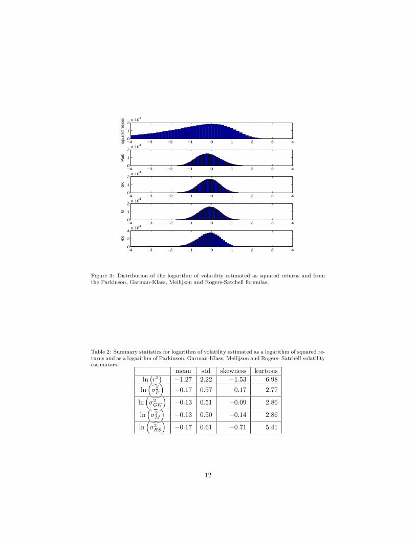
In the end, we investigate the distribution of ln σ2 (see Figure 3). As wecan see, the logarithm of the squared returns is highly nonnormally distributed,but the logarithms of the range-based volatility estimators have distributionssimilar to the normal distribution. To see the difference among various range-based estimators, we again calculate their summary statistics (see Table 2).

Note that the true volatility is normalized to one. Normality of the estimatoris desirable for practical reasons and therefore the ideal estimator should have

11

−4 −3 −2 −1 0 1 2 3 40

1

2x 10

4

squa

red

retu

rns

−4 −3 −2 −1 0 1 2 3 40

1

2x 10

4

Park

−4 −3 −2 −1 0 1 2 3 40

1

2x 10

4

GK

−4 −3 −2 −1 0 1 2 3 40

1

2x 10

4

M

−4 −3 −2 −1 0 1 2 3 40

2

4x 10

4

RS

Figure 3: Distribution of the logarithm of volatility estimated as squared returns and fromthe Parkinson, Garman-Klass, Meilijson and Rogers-Satchell formulas.

Table 2: Summary statistics for logarithm of volatility estimated as a logarithm of squared re-turns and as a logarithm of Parkinson, Garman-Klass, Meilijson and Rogers- Satchell volatilityestimators.

mean std skewness kurtosis

ln(r2)

−1.27 2.22 −1.53 6.98

ln(σ2P

)−0.17 0.57 0.17 2.77

ln(σ2GK

)−0.13 0.51 −0.09 2.86

ln(σ2M

)−0.13 0.50 −0.14 2.86

ln(σ2RS

)−0.17 0.61 −0.71 5.41

12

mean and skewness equal to zero, kurtosis close to three and standard deviationas small as possible. We see that from the five studied estimators the Garman-Klass and Meilijson volatility estimators, in addition to being most efficient,have best distributional properties.

3.3. Normality of normalized returns

As was empirically shown by Andersen, Bollerslev, Diebold, Labys (2000),Andersen, Bollerslev, Diebold, Ebens (2001), Forsberg and Bollerslev (2002) andThamakos and Wang (2003) on different data sets, standardized returns (returnsdivided by their standard deviations) are approximately normally distributed.In other words, daily returns can be written as

ri = σizi (32)

where zi ∼ N (0, 1). This finding has important practical implications too. Ifreturns (conditional on the true volatility) are indeed Gaussian and heavy tailsin their distributions are caused simply by changing volatility, then what we needthe most is a thorough understanding of the time evolution of volatility, possiblyincluding the factors which influence it. Even though the volatility models areused primarily to capture time evolution of volatility, we can expect that thebetter our volatility models, the less heavy-tailed distribution will be neededfor modelling of the stock returns. This insight can contribute to improvedunderstanding of volatility models, which is in turn crucial for risk management,derivative pricing, portfolio management etc.

Intuitively, normality of the standardized returns follows from the CentralLimit Theorem: since daily returns are just a sum of high-frequency returns,daily returns will be drawn from normal distribution.7

Since both this intuition and the empirical evidence of the normality of re-turns standardized by their standard deviations is convincing, it is appealing torequire that one of the properties of a ”good” volatility estimator should be thatreturns standardized by standard deviations obtained from this estimator willbe normally distributed (see e.g. Bollen and Inder (2002)). However, this intu-ition is not correct. As I now show, returns standardized by some estimate of thetrue volatility do not need to, and generally will not, have the same propertiesas returns standardized by the true volatility. Therefore we need to understandwhether the range-based volatility estimators are suitable for standardization ofthe returns. There are two problems associated with these volatility estimators:they are noisy and their estimates might be (and typically are) correlated withreturns. These two problems might cause returns standardized by the estimatedstandard deviations not to be normal, even when the returns standardized bytheir true standard deviations are normally distributed.

7given the limited time-dependence and some conditions on existence of moments.

13

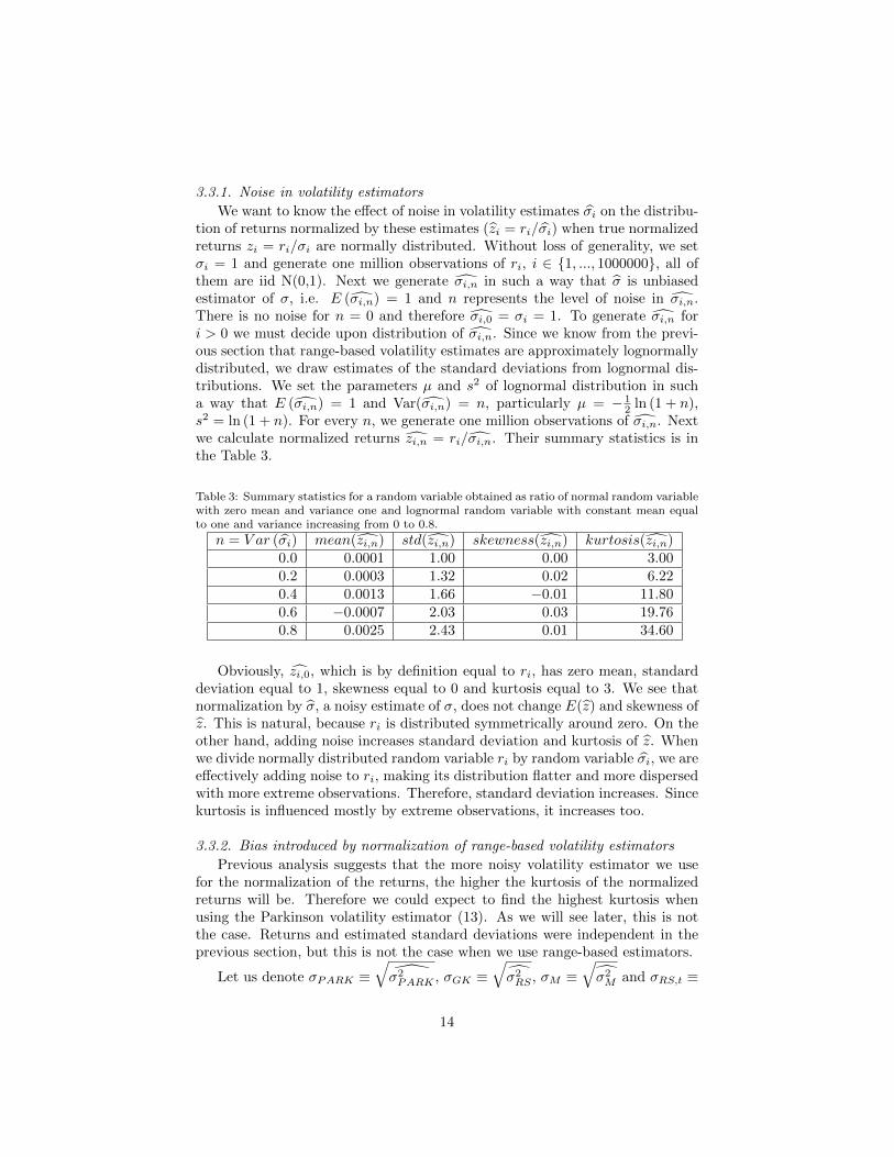
3.3.1. Noise in volatility estimators

We want to know the effect of noise in volatility estimates σi on the distribu-tion of returns normalized by these estimates (zi = ri/σi) when true normalizedreturns zi = ri/σi are normally distributed. Without loss of generality, we setσi = 1 and generate one million observations of ri, i ∈ {1, ..., 1000000}, all ofthem are iid N(0,1). Next we generate σi,n in such a way that σ is unbiasedestimator of σ, i.e. E (σi,n) = 1 and n represents the level of noise in σi,n.There is no noise for n = 0 and therefore σi,0 = σi = 1. To generate σi,n fori > 0 we must decide upon distribution of σi,n. Since we know from the previ-ous section that range-based volatility estimates are approximately lognormallydistributed, we draw estimates of the standard deviations from lognormal dis-tributions. We set the parameters µ and s2 of lognormal distribution in sucha way that E (σi,n) = 1 and Var(σi,n) = n, particularly µ = − 1

2 ln (1 + n),s2 = ln (1 + n). For every n, we generate one million observations of σi,n. Nextwe calculate normalized returns zi,n = ri/σi,n. Their summary statistics is inthe Table 3.

Table 3: Summary statistics for a random variable obtained as ratio of normal random variablewith zero mean and variance one and lognormal random variable with constant mean equalto one and variance increasing from 0 to 0.8.

n = V ar (σi) mean(zi,n) std(zi,n) skewness(zi,n) kurtosis(zi,n)0.0 0.0001 1.00 0.00 3.000.2 0.0003 1.32 0.02 6.220.4 0.0013 1.66 −0.01 11.800.6 −0.0007 2.03 0.03 19.760.8 0.0025 2.43 0.01 34.60

Obviously, zi,0, which is by definition equal to ri, has zero mean, standarddeviation equal to 1, skewness equal to 0 and kurtosis equal to 3. We see thatnormalization by σ, a noisy estimate of σ, does not change E(z) and skewness ofz. This is natural, because ri is distributed symmetrically around zero. On theother hand, adding noise increases standard deviation and kurtosis of z. Whenwe divide normally distributed random variable ri by random variable σi, we areeffectively adding noise to ri, making its distribution flatter and more dispersedwith more extreme observations. Therefore, standard deviation increases. Sincekurtosis is influenced mostly by extreme observations, it increases too.

3.3.2. Bias introduced by normalization of range-based volatility estimators

Previous analysis suggests that the more noisy volatility estimator we usefor the normalization of the returns, the higher the kurtosis of the normalizedreturns will be. Therefore we could expect to find the highest kurtosis whenusing the Parkinson volatility estimator (13). As we will see later, this is notthe case. Returns and estimated standard deviations were independent in theprevious section, but this is not the case when we use range-based estimators.

Let us denote σPARK ≡√σ2PARK , σGK ≡

√σ2RS , σM ≡

√σ2M and σRS,t ≡

14

−3 −2 −1 0 1 2 30

1

2x 10

4

true

−3 −2 −1 0 1 2 30

5000

10000

PA

RK

−3 −2 −1 0 1 2 3012

x 104

GK

−3 −2 −1 0 1 2 30

5000

10000

M

−3 −2 −1 0 1 2 3024

x 104

RS

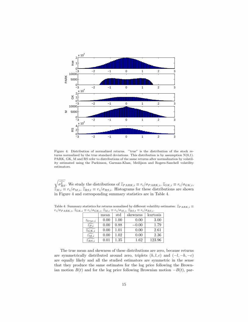
Figure 4: Distribution of normalized returns. ”true” is the distribution of the stock re-turns normalized by the true standard deviations. This distribution is by assumption N(0,1).PARK, GK, M and RS refer to distributions of the same returns after normalization by volatil-ity estimated using the Parkinson, Garman-Klass, Meilijson and Rogers-Sanchell volatilityestimators.

√σ2RS . We study the distributions of zPARK,i ≡ ri/σPARK,i, zGK,i ≡ ri/σGK,i,

zM,i ≡ ri/σM,i, zRS,t ≡ ri/σRS,i. Histograms for these distributions are shownin Figure 4 and corresponding summary statistics are in Table 4.

Table 4: Summary statistics for returns nomalized by different volatility estimates: zPARK,i ≡ri/σPARK,i, zGK,i ≡ ri/σGK,i, zM,i ≡ ri/σM,i, zRS,t ≡ ri/σRS,i.

mean std skewness kurtosisztrue,i 0.00 1.00 0.00 3.00zP,i 0.00 0.88 −0.00 1.79zGK,i 0.00 1.01 0.00 2.61zM,i 0.00 1.02 0.00 2.36zRS,i 0.01 1.35 1.62 123.96

The true mean and skewness of these distributions are zero, because returnsare symmetrically distributed around zero, triplets (h, l, c) and (−l,−h,−c)are equally likely and all the studied estimators are symmetric in the sensethat they produce the same estimates for the log price following the Brown-ian motion B(t) and for the log price following Brownian motion −B(t), par-

15

ticularly σPARK (h, l, c) = σPARK (−l,−h, c), σGK (h, l, c) = σGK (−l,−h, c),σM (h, l, c) = σM (−l,−h, c) and σRD (h, l, c) = σRS (−l,−h, c).

However, it seems from Table 4 that distribution of zRS,i is skewed. Thereis another surprising fact about zRS,i. It has very heavy tails. The reason forthis is that the formula (20) is derived without the assumption of zero drift.Therefore, when stock price performs one-way movement, this is attributed tothe drift term and volatility is estimated to be zero. (If movement is mostly inone direction, estimated volatility will be nonzero, but very small). Moreover,this is exactly the situation when stock returns are unusually high. Dividingthe largest returns by the smallest estimated standard deviations causes a lotof extreme observations and therefore very heavy tails. Due to these extremeobservations the skewness of the simulated sample is different from the skew-ness of the population, which is zero. This illustrates that the generality (driftindependence) of the Rogers and Satchell (1991) volatility estimator actuallyworks against this estimator in cases when the drift is zero.

When we use the Parkinson volatility estimator for the standardization ofthe stock returns, we get exactly the opposite result. Kurtosis is now muchsmaller than for the normal distribution. This is in line with empirical findingof Bollen and Inder (2002). However, this result should not be interpreted thatthis estimator is not working properly. Remember that we got the result ofthe kurtosis being significantly smaller than 3 under ideal conditions, when theParkinson estimator works perfectly (in the sense that it works exactly as it issupposed to work). Remember that this estimator is based on the range. Eventhough the range, which is based on high and low prices, seems to be independentof return, which is based on the open and close prices, the opposite is the case.Always when return is high, range will be relatively high too, because range isalways at least as large as absolute value of the return. |r| /σPARK will neverbe larger than

√4 ln 2, because

|r|σPARK

=|r|h−l√4 ln 2

=√

4 ln 2|r|h− l

≤√

4 ln 2 (33)

The correlation between |r| and σPARK is 0.79, what supports our argument.Another problem is that the distribution of zP,i is bimodal.

As we can see from the histogram, distribution of zM,i does not have any tailseither. This is because the Meilijson volatility estimator suffers from the sametype of problem as the Parkinson volatility estimator, just to a much smallerextent.

The Garman-Klass volatility estimator combines the Parkinson volatility es-timator with simple squared return. Even though both, the Parkinson estimatorand squared return are highly correlated with size of the return, the overall effectpartially cancels out, because these two quantities are subtracted. Correlationbetween |r| and σGK is indeed only 0.36. zGK,i has approximately normal dis-tribution, as the effect of noise and the effect of correlation with returns to largeextent cancels out.

We conclude this subsection with the appeal that we should be aware of the

16

assumptions behind the formulas we use. As range-based volatility estimatorswere derived to be as precise volatility estimators as possible, they work well forthis purpose. However, there is no reason why all of these estimators should workproperly when used for the standardization of the returns. We conclude thatfrom the studied estimators the only estimator appropriate for standardizationof returns is the Garman-Klass volatility estimator. We use this estimator laterin the empirical part.

3.4. Jump component

So far in this paper, returns and volatilities were related to the trading day,i.e. the period from the open to the close of the market. However, most ofthe assets are not traded continuously for 24 hours a day. Therefore, openingprice is not necessarily equal to the closing price from the previous day. We areinterested in daily returns

ri = ln(Ci)− ln(Ci−1) (34)

simply because for the purposes of risk management we need to know the totalrisk over the whole day, not just the risk of the trading part of the day. If we donot adjust range-based estimators for the presence of opening jumps, they willof course underestimate the true volatility. The Parkinson volatility estimatoradjusted for the presence of opening jumps is

σ2P =

(h− l)2

4 ln 2+ j2 (35)

where ji = ln(Oi)− ln(Ci−1) is the opening jump. The jump-adjusted Garman-Klass volatility estimator is:

σ2GK = 0.5 (h− l)2 − (2 ln 2− 1) c2 + j2 (36)

Other estimators should be adjusted in the same way. Unfortunately, includingopening jump will increase variance of the estimator when opening jumps aresignificant part of daily returns.8 However, this is the only way how to getunbiased estimator without imposing some additional assumptions. If we knewwhat part of the overall daily volatility opening jumps account for, we could findoptimal weights for the jump volatility component and for the volatility withinthe trading day to minimize the overall variance of the composite estimator.This is done in Hansen and Lunde (2005), who study how to combine openingjump and realized volatility estimated from high frequency data into the mostefficient estimator of the whole day volatility. However, the relation of openingjump and the trading day volatility can be obtained only from data. Moreover,there is no obvious reason why the relationship from the past should hold in the

8Jump volatility is estimated with smaller precision than volatility within trading day.

17

future. Simply adding jump component makes range-based estimators unbiasedwithout imposing any additional assumption.9

Adjustment for an opening jump is not as obvious as it seems to be and evenresearchers quite often make mistakes when dealing with this issue. The mostcommon mistake is that the range-based volatility estimators are not adjustedfor the presence of opening jumps at all (see e.g. Parkinson volatility estimatorin Bollen, Inder (2002)). A less common mistake, but with worse consequencesis an incorrect adjustment for the opening jumps. E.g. Bollen and Inder (2002)and Fiess and MacDonald (2002) refer to the following formula

σ2GKwrong,i = 0.5 (lnHi − lnLi)

2 − (2 ln 2− 1) (lnCi − lnCi−1)2

(37)

as Garman-Klass formula. This ”Garman-Klass volatility estimator” will onaverage be even smaller than a Garman-Klass estimator not adjusted for jumps.Moreover, it sometimes produces negative estimates for volatility (variance σ2).

4. Normalized returns - empirics

Andersen, Bollerslev, Diebold, and Ebens (2001) find that ”although the un-conditional daily return distributions are leptokurtic, the daily returns normal-ized by the realized standard deviations are close to normal.” Their conclusionis based on standard deviations obtained these from high frequency data. Westudy whether (and to what extend) this result is obtainable when standarddeviations are estimated from daily data only.

We study stocks which were the components of the Dow Jow IndustrialAverage on January 1, 2009, namely AA, AXP, BA, BAC, C, CAT, CVX,DD, DIS, GE, GM, HD, HPQ, IBM, INTC, JNJ, JPM, CAG10, KO, MCD,MMM, MRK, SFT, PFE, PG, T, UTX, VZ and WMT. We use daily open,high, low and close prices. The data covers years 1992 to 2008. Stock prices areadjusted for stock splits and similar events. We have 4171 daily observationsfor every stock. These data were obtained from the CRSP database. We studyDJI components to make our results as highly comparable as possible with theresults of Andersen, Bollerslev, Diebold, and Ebens (2001).

For brevity, we study only two estimators: the Garman-Klass estimator (15)and the Parkinson estimator (13). We use the Garman-Klass volatility estimatorbecause our previous analysis shows that it is the most appropriate one. Weuse the Parkinson volatility estimator to demonstrate that even though thisestimator is the most commonly used range-based estimator, it should not beused for normalization of returns. Moreover, we study the effect of including orexcluding a jump component into range-based volatility estimators.

9These assumptions could be based on past data, but they would still be just assumptions.10Since historical data for KFT (component of DJI) are not available for the complete

period, we use its biggest competitor CAG instead.

18

First of all, we need to distinguish the daily returns and the trading dayreturns. By the daily returns we mean close-to-close returns, calculated ac-cording to formula (34). By the trading day returns we mean returns duringthe trading hours, i.e. open-to-close returns, calculated according to formula(2). We estimate volatilities accordingly: volatility of the trading day returnsfrom (13) and (15) and the volatility of the daily returns using (35) and (36).Next we calculate standardized returns. We calculate standardized returns inthree different ways: trading day returns standardized by trading day standarddeviations (square root of trading day volatility), daily returns standardized bydaily standard deviation and daily returns standardized by trading day stan-dard deviation. Why do we investigate daily returns standardized by trading daystandard deviations too? Theoretically, this does not make much sense becausethe return and the standard deviations are related to different time intervals.However, it is still quite common (see e.g. Andersen, Bollerslev, Diebold, andEbens (2001)), because people are typically interested in daily returns, but thedaily volatility cannot be estimated as precisely as trading day volatility. Thevolatility of the trading part of the day can be estimated very precisely fromthe high frequency data, whereas estimation of the daily volatility is alwaysless precise because of the necessity of including the opening jump component.Therefore, trading day volatility is commonly used as a proxy for daily volatil-ity. This approximation is satisfactory as long as the opening jump is small incomparison to trading day volatility, which is typically the case.

Now we calculate summary statistics for the different standardized returnsas well as returns themselves. Results for the standard deviations are presentedin Table 5 and results for the kurtosis are presented in Table 6. We do not putsimilar tables for mean and kurtosis into this paper, because these results areless interesting and can be summarized in one sentance: Mean returns are alwaysvery close to zero, independent of which standardization we used. Skewness isalways very close to zero too.

The results for standard deviations and kurtosis are generally in line with thepredictions from our simulations too. First let us discuss the standard deviationsof the standardized returns. As Table 5 documents, normalization by standarddeviations obtained from the Parkinson volatility estimator results in standarddeviation smaller than one, approximately around 0.9 whereas normalization bystandard deviation obtained from the Garman-Klass volatility estimator resultsin standard deviations larger than one, around 1.05. Normalization by standarddeviations estimated from GARCH model is approximately 1.1. This is expectedas well, because division by a noisy random variable increases the standarddeviation.

Results for the kurtosis of standardized returns (see Table 6) are in linewith the predictions from our simulations too. Return distributions have heavytails (kurtosis significantly larger than 3). Second, the daily returns normalizedby the standard deviations calculated from Garman-Klass formula are closeto normal (kurtosis is close to 3). Third, the daily returns normalized by thestandard deviations calculated from Parkinson formula have no tails (kurtosis issignificantly smaller than 3). Fourth, normalization of daily returns by standard

19

Table 5: Standard deviations of the stock returns. rtd is an open-to-close return, rd is a close-to-close return. σGK,td (σP,td) is square root of Garman-Klass (Parkinson) volatility estimatewithout opening jump component. σGK,d (σP,d) is square root of Garman-Klass (Parkinson)volatility estimate including opening jump component. σgarch is standard deviation estimatedfrom GARCH(1,1) model based on daily returns.

trading day returns daily returnsrtd

rtdσGK,td

rtdσP,td

rdrd

σGK,d

rdσP,d

rdσGK,td

rdσP,td

rdσgarch

AA 0.02 1.14 0.94 0.02 1.11 0.96 1.00 1.28 1.12AXP 0.02 1.11 0.92 0.02 1.07 0.94 1.00 1.26 1.11BA 0.02 1.04 0.89 0.02 1.02 0.92 1.00 1.20 1.10

BAC 0.02 1.12 0.93 0.02 1.08 0.94 1.00 1.26 1.12C 0.02 1.11 0.91 0.03 1.05 0.92 1.01 1.26 1.12

CAT 0.02 1.10 0.92 0.02 1.08 0.95 1.00 1.28 1.13CVX 0.01 1.11 0.92 0.02 1.08 0.95 1.00 1.25 1.09DD 0.02 1.07 0.90 0.02 1.02 0.91 1.00 1.18 1.06DIS 0.02 1.03 0.88 0.02 0.99 0.90 1.00 1.18 1.09GE 0.02 1.07 0.91 0.02 1.03 0.93 1.00 1.20 1.09GM 0.02 1.10 0.92 0.03 1.08 0.95 1.00 1.27 1.13HD 0.02 1.06 0.90 0.02 1.02 0.92 1.00 1.20 1.10

HPQ 0.02 1.08 0.91 0.03 1.04 0.92 1.00 1.23 1.11IBM 0.02 1.07 0.91 0.02 1.04 0.93 1.00 1.25 1.13

INTC 0.02 1.08 0.92 0.03 1.06 0.95 1.00 1.31 1.19JNJ 0.01 1.06 0.89 0.02 1.00 0.90 1.00 1.17 1.06JPM 0.02 1.06 0.90 0.02 1.03 0.92 1.00 1.22 1.10CAG 0.01 1.09 0.89 0.02 0.98 0.87 1.00 1.15 1.01KO 0.01 1.03 0.88 0.02 0.99 0.89 1.00 1.15 1.04

MCD 0.02 1.04 0.89 0.02 0.99 0.89 1.00 1.15 1.05MMM 0.01 1.05 0.89 0.02 1.02 0.90 1.00 1.16 1.04MRK 0.02 1.05 0.89 0.02 1.01 0.91 1.00 1.20 1.09MSFT 0.02 1.04 0.90 0.02 1.03 0.93 1.00 1.24 1.14PFE 0.02 1.08 0.91 0.02 1.04 0.92 1.00 1.22 1.10PG 0.01 1.07 0.90 0.02 1.01 0.90 1.00 1.17 1.05T 0.02 1.09 0.91 0.02 1.05 0.92 1.00 1.20 1.06

UTX 0.02 1.08 0.91 0.02 1.05 0.93 1.00 1.22 1.09VZ 0.02 1.08 0.91 0.02 1.04 0.92 1.00 1.21 1.08

WMT 0.02 1.04 0.88 0.02 1.01 0.90 1.00 1.20 1.08XOM 0.01 1.08 0.91 0.02 1.06 0.94 1.00 1.22 1.08

mean 0.02 1.07 0.90 0.02 1.04 0.92 1.00 1.22 1.09

20

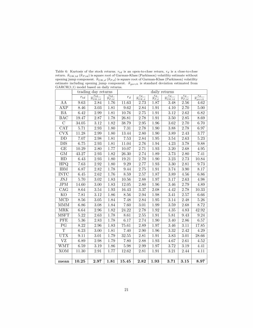
Table 6: Kurtosis of the stock returns. rtd is an open-to-close return, rd is a close-to-closereturn. σGK,td (σP,td) is square root of Garman-Klass (Parkinson) volatility estimate withoutopening jump component. σGK,d (σP,d) is square root of Garman-Klass (Parkinson) volatilityestimate including opening jump component. σgarch is standard deviation estimated fromGARCH(1,1) model based on daily returns.

trading day returns daily returnsrtd

rtdσGK,td

rtdσP,td

rdrd

σGK,d

rdσP,d

rdσGK,td

rdσP,td

rdσgarch

AA 9.63 2.84 1.76 11.63 2.73 1.87 3.48 2.56 4.62AXP 8.46 3.03 1.81 9.62 2.84 1.91 4.10 2.70 5.00BA 6.42 2.99 1.81 10.76 2.75 1.91 3.12 2.62 6.82

BAC 19.47 2.87 1.78 26.81 2.78 1.91 3.50 2.85 8.69C 34.05 3.12 1.82 38.79 2.95 1.96 3.62 2.70 6.70

CAT 5.71 2.93 1.80 7.31 2.78 1.90 3.88 2.78 6.97CVX 11.28 2.99 1.80 13.44 2.80 1.90 3.89 2.43 3.77DD 7.07 2.98 1.81 7.53 2.84 1.95 3.54 2.63 5.23DIS 6.75 2.93 1.81 11.04 2.76 1.94 4.23 3.78 9.88GE 10.29 2.80 1.77 10.07 2.71 1.93 3.20 2.68 4.95GM 43.27 2.93 1.82 26.30 2.74 1.89 3.73 2.80 7.41HD 6.43 2.93 1.80 19.21 2.70 1.90 3.23 2.73 10.84

HPQ 7.63 2.92 1.80 9.29 2.77 1.93 3.30 2.81 9.73IBM 6.87 2.82 1.78 9.44 2.75 1.91 3.74 3.90 8.17

INTC 6.45 2.62 1.76 8.59 2.57 1.87 3.89 4.56 6.86JNJ 5.70 3.02 1.83 10.56 2.88 1.97 3.17 2.63 4.98JPM 14.60 3.00 1.83 12.05 2.80 1.96 3.46 2.79 4.89CAG 8.64 3.54 1.93 16.43 3.37 2.08 4.42 2.78 10.33KO 7.81 3.12 1.86 8.56 2.94 1.98 3.41 2.57 6.66

MCD 8.56 3.05 1.84 7.48 2.84 1.95 3.14 2.48 5.26MMM 6.86 3.08 1.84 7.60 3.01 1.99 3.59 2.68 8.72MRK 6.64 2.96 1.82 24.22 2.78 1.92 4.35 4.83 42.92MSFT 5.22 2.63 1.78 8.61 2.55 1.91 5.81 9.43 9.24PFE 5.36 2.83 1.78 6.17 2.74 1.90 3.40 2.86 6.57PG 8.22 2.96 1.83 75.61 2.89 1.97 3.46 3.11 17.85T 6.23 3.00 1.81 7.40 2.90 1.96 3.32 2.42 4.29

UTX 9.11 3.01 1.79 32.55 2.81 1.91 3.83 3.01 28.66VZ 6.89 2.98 1.79 7.80 2.88 1.93 4.67 2.61 4.52

WMT 6.59 3.19 1.86 5.98 2.99 1.97 3.72 3.19 4.41XOM 11.30 2.91 1.77 12.62 2.81 1.91 3.21 2.44 4.11

mean 10.25 2.97 1.81 15.45 2.82 1.93 3.71 3.15 8.97

21

deviation estimated for trading day only, will cause upward bias in kurtosis.This is a consequence of the standardization by an incorrect standard deviation- sometimes (particularly in a situation when the opening jump is large), returnsare divided by too small standard deviation, which will cause too many largeobservations for normalized returns.

The last column of Table 6 reports kurtosis of returns normalized by stan-dard deviations estimated from GARCH(1,1) model with mean return fixed tozero. As we can see, these normalized returns are not Gaussian, they havefat tails. This is consistent with the fact that GARCH models with fat-tailedconditional distribution of returns fit data better than GARCH models withconditionally normally distributed returns. However, as is clear from this pa-per, this is the case simply because GARCH models always condition returndistribution on the estimated volatility, which is only a noisy proxy of the truevolatility. Therefore, even when distribution of returns conditional on the truevolatility is Gaussian, distribution of returns conditional on estimated volatilitywill have heavy tails. This result has an important implication for volatilitymodelling: the more precisely we can estimate the volatility, the closer will bethe conditional distribution of returns to the normal distribution.

5. Conclusion

Range-based volatility estimators provide significant increase in accuracycompared to simple squared returns. Even though efficiency of these estimatorsis known, there is some confusion about other properties of these estimators. Westudy these properties. Our main focus is the properties of returns standardizedby their standard deviations.

First, we correct some mistakes in existing literature. Second, we studydifferent properties of range-based volatility estimators and find that for mostpurposes, the best volatility estimators is the Garman-Klass volatility estimator.The Meilijson volatility estimator improves its efficiency slightly, but it is basedon a significantly more complicated formula. However, performance of all therange-based volatility estimators is similar in most cases except for the casewhen we want to use them for standardization of the returns.

Returns standardized by their standard deviations are known to be normallydistributed. This fact is important for the volatility modelling. This result waspossible to obtain only when the standard deviations were estimated from thehigh frequency data. When the standard deviations were obtained from volatil-ity models based on daily data, returns standardized by these standard devia-tions are not Gaussian anymore, they have heavy tails. Using simulations weshow that even when returns themselves are normally distributed, returns stan-dardized by (imprecisely) estimated volatility are not normally distributed; theirdistribution has heavy tails. In other words: the fact that standard volatilitymodels show that even conditional distribution of returns has heavy tails doesnot mean that returns are not normally distributed. It means that these mod-els cannot estimate volatility precisely enough and the noise in the volatilityestimates causes the heavy tails.

22

It is not obvious whether range-based volatility estimators can be used for thestandardization of the returns. Using simulations we find that for the purpose ofreturns standardization there are large differences between these estimators andwe find that the Garman-Klass volatility estimator is the only one appropriatefor this purpose. Putting all the results together, we rate the Garman-Klassvolatility estimator as the best volatility estimator based on daily (open, high,low and close) data. We test this estimator empirically and we find that we canindeed obtain basically the same results from daily data as Andersen, Bollerslev,Diebold, and Ebens (2001) obtained from high-frequency (transaction) data.This is important, because the high-frequency data are very often not availableor available only for a shorter time period and their processing is complicated.Since returns scaled by standard deviations estimated from GARCH type ofmodels (based on daily returns) are not Gaussian (they have fat tails), ourresults show that the GARCH type of models cannot capture the volatilityprecisely enough. Therefore, in the absence of high-frequency data, furtherdevelopment of volatility models based on open, high, low and close prices isrecommended.

[1] Alizadeh, S., Brandt, M. W., & Diebold, F. X. (2002). Range-based esti-mation of stochastic volatility models. Journal of Finance, 57, 1047–1091.

[2] Andersen T. G., Bollerslev T., Diebold F.X., & Labys, P. (2000). Exchangerate returns standardized by realized volatility are nearly Gaussian. Multi-national Finance Journal, 4, 159–179.

[3] Andersen, T. G., Bollerslev, T. Diebold F.X. & Ebens, H. (2001). The dis-tribution of realized stock return volatility. Journal of Financial Economics,61, 43–76.

[4] Bali, T. G., & Weinbaum, D. (2005). A comparative study of alternativeextreme-value volatility estimators. Journal of Futures Markets, 25, 873–892.

[5] Bernard Bollen, B., & Inder, B. (2002). Estimating daily volatility in fi-nancial markets, Journal of Empirical Finance, 9, 551–562.

[6] Brandt, M. W., & Diebold, F. X. 2006. A no-arbitrage approach to rangebased estimation of return covariances and correlations. Journal of Busi-ness, 79, 61–74.

[7] Brandt, M. W., & Jones., Ch. S. (2006). Volatility forecasting with Range-Based EGARCH models. Journal of Business and Economic Statistics, 24(4), 470–486.

[8] Broto, C. & Ruiz, E. (2004), Estimation methods for stochastic volatilitymodels: a survey. Journal of Economic Surveys, 18, 613–649.

[9] Chou, R. Y. (2005) Forecasting financial volatilities with extreme values:the conditional autoregressive range (CARR) model. Journal of Money,Credit and Banking, 37 (3), 561–582.

23

[10] Chou, R. Y., 2006. Modeling the asymmetry of stock movements usingprice ranges. Advances in Econometrics, 20, 231–258.

[11] Chou, R. Y., Chou, H., & Liu, N. (2010). Range volatility models andtheir applications in finance. Handbook of Quantitative Finance and RiskManagement, Chapter 83, Springer.

[12] Chou, R. Y., & Liu, N. (2010). The economic value of volatility timing usinga range-based volatility model. Journal of Economic Dynamics & Control,34, 2288–2301.

[13] Dacorogna, M. M., Gencay, R., Muller, U. A., Olsen, R. B., & Pictet, O. V.(2001). An Introduction to High-Frequency Finance. San Diego: AcademicPress.

[14] Feller, W. (1951). The asymptotic distribution of the range of sums ofindependent random variables. The Annals of Mathematical Statistics, 22,427–432.

[15] Fiess, N. M., & MacDonald, R. (2002). Towards the fundamentals of tech-nical analysis: analysing the information content of High, Low and Closeproces. Economic Modelling, 19, 354–374.

[16] Forsberg, L., & Bollerslev, T. (2002). Bridging the gap between the dis-tribution of realized (ECU) volatility and ARCH modelling (of the Euro):the GARCH-NIG model. Journal of Applied Econometrics, 17, 535–548.

[17] Garman, M. B., & Klass, M. J. (1980). On the Estimation of Security PriceVolatilities from Historical Data. The Journal of Business, 53 (1), 67–7

[18] Hansen, P. R., & Lunde, A. (2005). A realized variance for the whole daybased on intermittent high-frequency data. Journal of Financial Economet-rics, 3, 525–554.

[19] Karatzas, I., & Shreve, S. E. (1991). Brownian Motion and Stochastic Cal-culus. New York: Springer-Verlag.

[20] Kunitomo, N. (1992). Improving the Parkinson method of estimating secu-rity price volatilities. Journal of Business, 65, 295–302.

[21] Meilijson, I., (2009), The Garman–Klass volatil-ity estimator revisited, working paper available at:http://arxiv.org/PS cache/arxiv/pdf/0807/0807.3492v2.pdf

[22] Parkinson, M. (1980). The extreme value method for estimating the vari-ance of the rate of return. Journal of Business, 53, 61–65.

[23] Rogers, L. C. G., & Satchell, S. E. (1991). Estimating variance from high,low and closing prices. Annals of Applied Probability, 1, 504–12.

24

[24] Thomakos, D. D., Wang, T., (2003), Realized volatility in the futures mar-kets. Journal of Empirical Finance, 10, 321–353.

[25] Yang, D., & Zhang, Q. (2000). Drift-independent volatility estimationbased on high, low, open, and close prices. Journal of Business, 73, 477–491.

25