Property Rights for the Poor: Effects of Land Titling

Sebastian Galiani Washington University in St Louis

Ernesto Schargrodsky*

Universidad Torcuato Di Tella

January 19, 2009

Abstract Secure property rights are considered a key determinant of economic development. The evaluation of the causal effects of property rights, however, is a difficult task as their allocation is typically endogenous. To overcome this identification problem, we exploit a natural experiment in the allocation of land titles. In 1981, squatters occupied a piece of land in a poor suburban area of Buenos Aires. In 1984, a law was passed expropriating the former owners’ land to entitle the occupants. Some original owners accepted the government compensation, while others disputed the compensation payment in the slow Argentine courts. These different decisions by the former owners generated an exogenous allocation of property rights across squatters. Using data from two surveys performed in 2003 and 2007, we find that entitled families substantially increased housing investment, reduced household size, and enhanced the education of their children relative to the control group. These effects, however, did not take place through improvements in access to credit. Our results suggest that land titling can be an important tool for poverty reduction, albeit not through the shortcut of credit access, but through the slow channel of increased physical and human capital investment, which should help to reduce poverty in the future generations. JEL: P14, Q15, O16, J13 Keywords: Property rights, land titling, natural experiment, urban poverty. * Sebastian Galiani, Department of Economics, Washington University in St Louis, Campus Box 1208, St Louis, MO 63130-4899, US, galiani@wustl.edu. Ernesto Schargrodsky, Universidad Torcuato Di Tella, Saenz Valiente 1010, (C1428BIJ) Buenos Aires, Argentina, eschargr@utdt.edu. We are grateful to seminar participants at the AEA meetings, NBER, Harvard, MIT, Stanford, Chicago, Yale, Berkeley, Columbia, UCLA, UCL, UC San Diego, Brown, Boston University, Washington in St. Louis, Essex, Miami, Econometric Society, ISNIE, Ronald Coase Institute, LACEA, NIP, Universidad de Chile, Universidad Getulio Vargas, PUC Rio, Universidad de Montevideo, UdeSA, UTDT, World Bank, and IADB for helpful comments. Alberto Farias and Daniel Galizzi provided crucial help throughout this study. We also thank Gestion Urbana -the NGO that performed the survey-, Eduardo Amadeo, Julio Aramayo, Rosalia Cortes, Maria de la Paz Dessy, Pedro Diaz, Alejandro Lastra, Hector Lucas, Graciela Montañez, Juan Sourrouille, and Ricardo Szelagowski for their cooperation; Matias Cattaneo, Sebastian Calonico and Florencia Borrescio Higa for excellent research assistance; the World Bank and the Inter-American Development Bank for financial support for our 2003 survey, and the Ronald Coase Institute for financial support for our 2007 survey.

1

I. Introduction

The fragility of property rights is considered a crucial obstacle for economic development

(North and Thomas, 1973; North, 1981; De Long and Shleifer, 1993; Acemoglu,

Johnson, and Robinson, 2001; Johnson, McMillan and Woodruff, 2002; inter alia). The

main argument is that individuals underinvest if others can seize the fruits of their

investments (Demsetz, 1967; Alchian and Demsetz, 1973). In today’s developing world,

a pervasive manifestation of feeble property rights are the millions of people living in

urban dwellings without possessing formal titles of the plots of land they occupy

(Deininger, 2003; and Banerjee and Duflo, 2006). The absence of formal property rights

constitutes a severe limitation for the poor. In addition to its investment effects, the lack

of formal titles impedes the use of land as collateral to access the credit markets (Feder

et al., 1988). It also affects the transferability of the parcels (Besley, 1995), making

investments in untitled parcels highly illiquid. Moreover, the absence of formal titles

deprives poor families of the possibility of having a valuable insurance and savings tool

that could provide protection during bad times and retirement, forcing them instead to

rely on extended family members and offspring as insurance mechanisms.

Land-titling programs have been recently advocated in policy circles as a powerful

intervention to rapidly reduce poverty. De Soto (2000) emphasizes that the lack of

property rights impedes the transformation of the wealth owned by the poor into capital.

Proper titling could allow the poor to collateralize the land. In turn, this credit could be

invested as capital in productive projects, promptly increasing labor productivity and

income. Inspired by these ideas, and fostered by international development agencies,

land-titling programs have been launched throughout developing and transition

economies as part of poverty alleviation efforts.

Several studies have documented the effects of land property rights and titling programs

on different variables. A partial listing includes Jimenez (1984), Alston et al. (1996) and

Lanjouw and Levy (2002) on real estate values; Besley (1995), Brasselle et al. (2002),

Field (2005), and Do and Iyer (2008) on investment; Banerjee et al. (2002) and Libecap

and Lueck (2008) on agricultural productivity, Field (2007) on labor supply; Feder et al.

(1988), Place and Migot-Adholla (1998), and Carter and Olinto (2002) on access to

credit, and Di Tella, Galiani and Schargrodsky (2007) on the formation of beliefs. We

2

contribute to this literature by exploiting a natural experiment in the allocation of property

rights to identify the causal effects of land titling on investment, access to credit, labor

market performance, household structure, and human capital accumulation.

The identification of land-titling effects is a difficult task because it typically faces the

problem that formal property rights are endogenous. The allocation of property rights

across households is usually not random but based on wealth, family characteristics,

individual effort, previous investment levels, or other mechanisms built on differences

between the groups that acquire those rights and the groups that do not. We understand

our natural experiment provides us with exogenous variability in the allocation of

property rights in order to solve this selection problem.

In 1981, a group of squatters occupied an area of wasteland in the outskirts of Buenos

Aires, Argentina. The area was composed of different tracts of land, each with a different

legal owner. An expropriation law was subsequently passed, ordering the transfer of the

land from the original owners to the state in exchange for a monetary compensation, with

the purpose of entitling it to the squatters. However, only some of the original legal

owners surrendered the land. The parcels located on the ceded tracts were transferred

to the squatters with legal titles that secured the property of the parcels. Other original

owners, instead, are still disputing the government compensation in the slow Argentine

courts. As a result, a group of squatters obtained formal land rights, while others are

currently living in the occupied parcels without paying rent, but without legal titles. Both

groups share the same household pre-treatment characteristics. Moreover, they live next

to each other, and the parcels they inhabit are identical. Since the decision of the original

owners of accepting or disputing the expropriation payment was orthogonal to the

squatter characteristics, the allocation of property rights is exogenous in equations

describing the behavior of the occupants. Thus, this natural experiment provides a

control group that estimates what would have happened to the treated group in the

absence of the intervention, allowing us to identify the causal effects of land titling.

Exploiting this natural experiment, we find significant effects on housing investment,

household size, and child education. The constructed surface increases by 12%, while

an overall index of housing quality rises by 37%. Moreover, households in the titled

parcels have a smaller size (an average of 5.11 members relative to 6.06 in the untitled

3

group), both through a diminished presence of extended family members and through a

reduced fertility of the household heads. In addition, the children from these smaller

households show significantly better educational achievement, with an average of 0.69

more years of schooling and twice the completion rate of secondary education (53% vs.

25%). However, we only find modest effects on access to credit markets as a result of

entitlement, and no improvement in labor market performance of the household heads.

Our results suggest that land titling can be an important tool for poverty reduction, albeit

not through the shortcut of credit access and entrepreneurial income, but through the

slow channel of increased physical and human capital investment.

The rest of the paper is organized as follows. In the next section we describe the natural

experiment. Section III describes our data, and section IV discusses the identification

methods. Section V presents our empirical results, while section VI concludes.

II. A Natural Experiment

The empirical evaluation of the effects of land titling poses a major methodological

challenge. The allocation of property rights across families is typically not random but

based on wealth, family characteristics, individual effort, previous investment levels, or

other selective mechanisms. Thus, the individual characteristics that determine the

likelihood of receiving land titles are probably correlated with the outcomes under study.

Since some of these personal characteristics are unobservable, this correlation creates a

selection problem that obstructs the proper evaluation of the effects of property right

acquisition.

In this paper, we address this selection problem by exploiting a natural experiment in the

allocation of property rights. In 1981, about 1,800 families occupied a piece of wasteland

in San Francisco Solano, County of Quilmes, in the Province of Buenos Aires, Argentina.

The occupants were groups of landless citizens organized through a Catholic chapel. As

they wanted to avoid creating a shantytown, they partitioned the occupied land into small

urban-shaped parcels. At the beginning of the occupation the squatters believed that the

land belonged to the state, but it was actually private property.1 The occupants resisted

1 This is explained by the squatters in the documentary movie “Por una tierra nuestra” by Cespedes (1984). On the details of the land occupation process also see Briante (1982), CEUR

4

several attempts of eviction during the military government. After Argentina's return to

democracy, the Congress of the Province of Buenos Aires passed Law Nº 10.239 in

1984 expropriating these lands from the former owners to allocate them to the squatters.

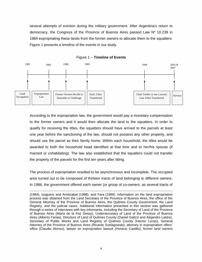
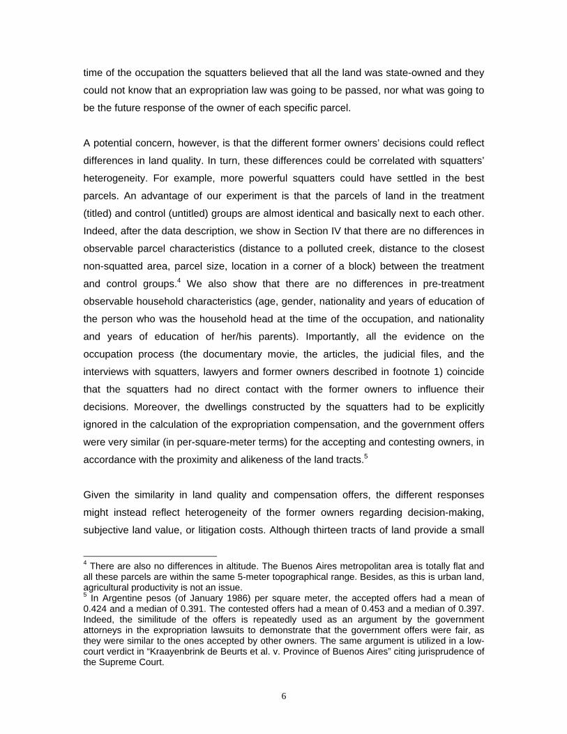
Figure 1 presents a timeline of the events in our study.

Figure 1 – Timeline of Events

According to the expropriation law, the government would pay a monetary compensation

to the former owners and it would then allocate the land to the squatters. In order to

qualify for receiving the titles, the squatters should have arrived to the parcels at least

one year before the sanctioning of the law, should not possess any other property, and

should use the parcel as their family home. Within each household, the titles would be

awarded to both the household head identified at that time and to her/his spouse (if

married or cohabitating). The law also established that the squatters could not transfer

the property of the parcels for the first ten years after titling.

The process of expropriation resulted to be asynchronous and incomplete. The occupied

area turned out to be composed of thirteen tracts of land belonging to different owners.

In 1986, the government offered each owner (or group of co-owners, as several tracts of (1984), Izaguirre and Aristizabal (1988), and Fara (1989). Information on the land expropriation process was obtained from the Land Secretary of the Province of Buenos Aires, the office of the General Attorney of the Province of Buenos Aires, the Quilmes County Government, the Land Registry, and the judicial cases. Additional information presented in this section was gathered through a series of interviews with key informants, including the Secretary of Land of the Province of Buenos Aires (Maria de la Paz Dessy), Undersecretary of Land of the Province of Buenos Aires (Alberto Farias), Directors of Land of Quilmes County (Daniel Galizzi and Alejandro Lastra), Secretary of Public Works and Land Registry of Quilmes County (Hector Lucas), General Attorney of the Province of Buenos Aires (Ricardo Szelagowski), attorney in expropriation offers’ office (Claudio Alonso), lawyer on expropriation lawsuit (Horacio Castillo), former land owners

Land Occupation

1984

Former Owners Decide to Surrender or Challenge

Surveys

Final Verdict in one Lawsuit. Late Titles Transferred.

Early Titles Transferred

1989 1986 1998 2003 & 2007

Expropriation Law

1981

5

land had more than one owner) a payment proportional to the official valuation of each

tract of land, indexed by inflation. These official valuations, assessed by the tax authority

to calculate property taxes, had been set before the land occupation. After the

government made the compensation offers, the owner/s of each tract had to decide

whether to surrender the land (accepting the expropriation compensation) or to start a

legal dispute. Eight former owners accepted the compensation offered by the

government. Five former owners, instead, did not accept the government offer and filed

charges with the aim of obtaining a higher compensation. In 1989, the tracts of land of

the former owners that accepted the government compensation were transferred to the

squatters occupying them, together with formal land titles that secured the property of

the parcels.2 The squatters that received titles in 1989 constitute the early-treated group

in our study.3

The people who occupied parcels located on the tracts of land that belonged to the

former owners that accepted the expropriation compensation, were ex-ante similar, and

arrived at the same time, than the people who settled on the tracts of the former owners

that did not surrender the land. There was simply no way for the occupants to know ex-

ante, at the time of the occupation, which parcels of land had owners who would accept

the compensation and which parcels had owners who would dispute it. In fact, at the (Hugo Spivak and Alejandro Bloise -heir-), squatters (Juan Carlos Sanchez and Jorge Valle, inter alia), and President of NGO Gestion Urbana (Estela Gutierrez). 2 The “new” urban design traced by the squatters differed from the previous land tract divisions. Thus, some “new” parcels overlapped over tracts of land that belonged to more than one former owner. This could be interpreted as further evidence of the squatters’ ignorance about the previous land ownership status. Had they known the existence of different private owners, they should have followed the previous land design to avoid being exposed to the decisions of two or three landowners rather than one. For regulatory reasons, parcels could not be delimited and titled if one portion of them was still under dispute. 3 The market value of land parcels comparable to the ones titled to the squatters amounted to approximately 7.4 times the monthly average total household income for the first quintile of the official household survey (EPH) of October 1986 for the Buenos Aires metropolitan area (market value of parcels in the neighboring non-squatted area obtained from evidence presented in “Kraayenbrink de Beurts et al. v. Province of Buenos Aires”). This figure, however, constitutes only an upper bound of the differential wealth transfer received by the entitled households for three reasons. First, the expropriation law established that each titled squatter had to pay the government the proportionally prorated share of the official valuation of the occupied tract of land. The law, however, established that the payments should be made in monthly installments that could never surpass 10% of the (observable) household income and there was no indexation for inflation. Given the hyperinflationary periods experienced by the Argentine economy during the period of analysis and the high labor informality of this population, the real values paid by the squatters were probably quite small. In practice, there are no records of the amounts and dates of the payments made by each household. Second, entitled households are supposed to regularly pay property taxes. Third, untitled squatters pay no rent.

6

time of the occupation the squatters believed that all the land was state-owned and they

could not know that an expropriation law was going to be passed, nor what was going to

be the future response of the owner of each specific parcel.

A potential concern, however, is that the different former owners’ decisions could reflect

differences in land quality. In turn, these differences could be correlated with squatters’

heterogeneity. For example, more powerful squatters could have settled in the best

parcels. An advantage of our experiment is that the parcels of land in the treatment

(titled) and control (untitled) groups are almost identical and basically next to each other.

Indeed, after the data description, we show in Section IV that there are no differences in

observable parcel characteristics (distance to a polluted creek, distance to the closest

non-squatted area, parcel size, location in a corner of a block) between the treatment

and control groups.4 We also show that there are no differences in pre-treatment

observable household characteristics (age, gender, nationality and years of education of

the person who was the household head at the time of the occupation, and nationality

and years of education of her/his parents). Importantly, all the evidence on the

occupation process (the documentary movie, the articles, the judicial files, and the

interviews with squatters, lawyers and former owners described in footnote 1) coincide

that the squatters had no direct contact with the former owners to influence their

decisions. Moreover, the dwellings constructed by the squatters had to be explicitly

ignored in the calculation of the expropriation compensation, and the government offers

were very similar (in per-square-meter terms) for the accepting and contesting owners, in

accordance with the proximity and alikeness of the land tracts.5

Given the similarity in land quality and compensation offers, the different responses

might instead reflect heterogeneity of the former owners regarding decision-making,

subjective land value, or litigation costs. Although thirteen tracts of land provide a small

4 There are also no differences in altitude. The Buenos Aires metropolitan area is totally flat and all these parcels are within the same 5-meter topographical range. Besides, as this is urban land, agricultural productivity is not an issue. 5 In Argentine pesos (of January 1986) per square meter, the accepted offers had a mean of 0.424 and a median of 0.391. The contested offers had a mean of 0.453 and a median of 0.397. Indeed, the similitude of the offers is repeatedly used as an argument by the government attorneys in the expropriation lawsuits to demonstrate that the government offers were fair, as they were similar to the ones accepted by other owners. The same argument is utilized in a low-court verdict in “Kraayenbrink de Beurts et al. v. Province of Buenos Aires” citing jurisprudence of the Supreme Court.

7

number for a statistical analysis, a few patterns emerge. The average number of co-

owners in the groups of accepting owners is 1.25, while the average number of co-

owners for the contested tracts is 2.2. Moreover, when we defined a dummy equal to 1 if

there is more than one co-owner sharing the same family name, and 0 otherwise, the

average for this dummy for the accepting owners is 0.125 while the average for the

challenging owners is 0.6. Thus, it appears that having many co-owners and several in

the same family made it more difficult for the owners to agree on accepting the

government offer.6 Note that if, in spite of this discussion, one may still fear that the

challenging owners did so because the unobservable quality of their land was higher,

that would imply that the squatters that did not receive titles are standing on land of

better quality.

As explained, five former owners did not accept the compensation offered by the

government and went to trial. In these lawsuits, all the legal discussion hinges around

the determination of the monetary compensation. The Congress constitutionally

approved the law and, thus, the expropriation itself could not be challenged. The

squatters had no participation in these legal processes (the lawsuits were exclusively

between the former owners and the provincial government), and the value of the

dwellings they constructed was explicitly excluded from the dispute over the monetary

compensation (“Cordar SRL v. Province of Buenos Aires”). One of these five lawsuits

ultimately ended with a final verdict, and the squatters on this tract of land received titles

in 1998 (the late treated). The other four lawsuits are still pending in the slow Argentine

courts. If one is still worried about the possibility that the former owners’ decisions of

surrendering or suing was correlated with land quality or squatters’ characteristics, then

an additional feature of this experience is that it allows us to separately compare the

squatters in this late-treated group relative to the control group. Although these two

groups of squatters settled in tracts of land which are homogenous regarding their

6 Kaplan et al. (2006) find that cases are less likely to be settled (more likely to go to court) when they involve multiple plaintiffs. See also Fiss (1984). On family economic decisions see, for example, Burkart et al. (2003) and Bennedsen et al. (2006). Within the challenging owners, we also found one case in which an owner was a lawyer who was representing himself in the case (which may suggest lower litigation costs), while in another case, one of the original owners had passed away before the sanctioning of the law but her inheritance process was still under way at the time the family had to make a decision.

8

respective former owners’ decisions of going to trial, one group already received titles

while the other is still waiting for the end of the legal processes.7

The final outcome of this expropriation process is that a group of families now has legal

property rights, while another group is still living in the occupied parcels enjoying free

usufructuary rights but without possessing formal land titles. This allocation of land titles

was the result of an expropriation process that did not depend on any particular

characteristic of the squatters nor of the parcels of land they occupied. Thus, by

comparing the groups that received and did not receive land titles, we can act as if we

have a randomized experiment.

III. Data Collection

The area affected by Expropriation Law Nº 10.239 covers a total of 1,839 parcels. 1,082

of these parcels are located in a contiguous set of blocks. However, the law also

included another non-contiguous (but close) piece of land currently called San Martin

neighborhood, which comprises 757 parcels. As this area is physically separated from

the rest, we focus on the 1,082 contiguous parcels to improve comparability.

We have precise knowledge of the titling status of each parcel. Land titles were awarded

in two phases. Property titles were awarded to the occupants of 419 parcels in 1989,

and to the occupants of 173 parcels in 1998. Land titles are not available to the families

living in 410 parcels located on tracts of land that have not been surrendered to the

government in the expropriation process. Finally, there are 80 parcels that were not titled

because the squatters occupying them had not fulfilled some of the required registration

steps, or had moved or died at the time of the title offers, although the original owners

had surrendered these pieces of land to the government. This subgroup constitutes the

7 We can still wonder, within this group of former owners that disputed the compensation, why some are still on trial while one concluded. Exogenous reasons lengthened the pending trials. In two cases, the expropriation lawsuit was delayed by the death of one of the former owners, which required an inheritance process. In another case (mentioned in footnote 6) one of the original owners had died just before the sanctioning of the law and her inheritance process had not finished. In the fourth case, the legal process was delayed by a mistake made in the description of the land tract in a low-court judge’s verdict.

9

“non-compliers” in our study, since they were offered the treatment (land title) but they

did not receive it.8

Two surveys performed in 2003 and 2007 provide the data utilized for this study. In

2003, the inhabitants of 590 randomly selected parcels (out of the total of 1,839) were

interviewed. 617 households living in these 590 parcels (27 parcels host more than one

family) were surveyed. Excluding the non-contiguous San Martin neighborhood, we

interviewed 467 households living in 448 parcels. The questionnaire covered

socioeconomic variables including household structure, labor market outcomes, and

credit information. At the same time, we sent a team of architects to measure housing

investments by performing an outside evaluation of the characteristics of the dwellings in

all the parcels.9

The 245 families in the contiguous area that were identified in the 2003 survey as having

arrived to the current parcels before the treatment assignment (see next section) and as

having offspring of the household head of 0-16 years of age, were the target of the 2007

survey. This second survey aimed to measure the school achievement of the sample of

701 children satisfying these conditions (who by then were between 4-20 years old) as

they progressed throughout the educational system. 217 of these 245 households (633

of these 701 children) were successfully re-interviewed.10

8 23 of these 80 parcels could have been titled in 1989, while the other 57 correspond to the group titled in 1998. The 757 parcels of San Martin, which belonged to an owner who accepted the expropriation compensation without suing, were offered for titling in 1991. 712 were titled, while 45 correspond to non-compliers. 9 Gestion Urbana, an NGO that works in this area, carried out the household survey and the housing evaluation. We distributed food stamps for each answered survey as a token of gratitude to the families willing to participate in our study. In 10 percent of the cases, the survey could not be performed because there was nobody at home in three visit attempts, the parcel was not used as a house, rejection, or other reasons. These parcels were randomly replaced. Non-response rates were similar for titled and untitled parcels. 10 The NGO Gestion Urbana also conducted the education survey, distributing again food stamps for each answered survey. Re-interviewing was greatly facilitated by our collection of exact name, date of birth, national ID number, address, and parents’ names for the offspring of the household heads in the first survey. Re-interview rates were similar for titled and untitled parcels. When a family had moved from their 2003 location, surveyors attempted to find the target family using the 2003 data and the information provided by the current occupants. 7 of the 217 families were interviewed in this way.

10

IV. Identification Strategy

We seek to identify the effect of the allocation of property rights on several outcome

variables exploiting a natural experiment in the allocation of land titling. In a natural

experiment, like in a randomized trial, there is a control group that estimates what would

have happened to the treated group in the absence of the intervention, but nature or

other exogenous forces determine treatment status instead. The validity of the control

group is evaluated by examining the exogeneity of treatment status with respect to the

potential outcomes, and by testing that the pre-intervention characteristics of the

treatment and control groups are reasonably similar. In section II we discussed at length

the process of allocation of land title offers and argued that this process was exogenous

to the characteristics of the squatters in our experiment. We now test the similarity of

pre-treatment characteristics between the treatment and control groups.

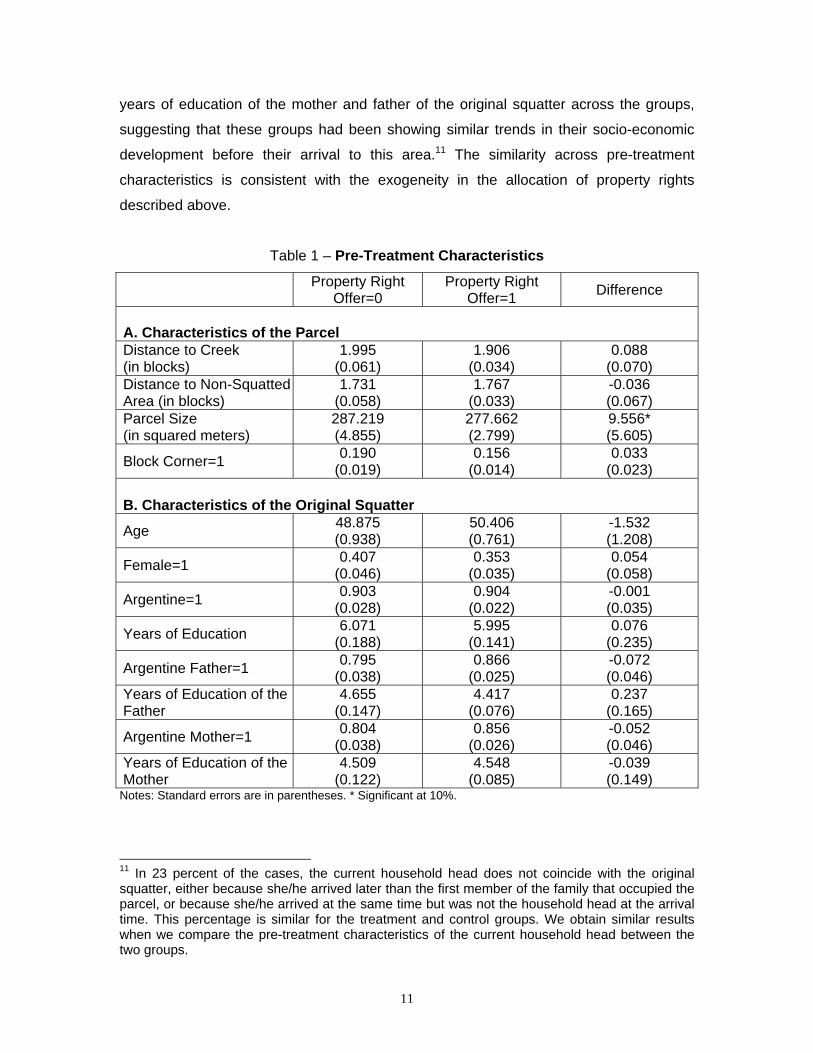
In Table 1, we compare pre-treatment characteristics for the non-intention-to-treat and

intention-to-treat groups to analyze the presence of potential differences. The variable

Property Right Offer equals 1 for the parcels that were surrendered by the original

owners, and 0 otherwise. In Panel A, we compare parcel characteristics: distance to a

nearby (polluted and floodable) creek, distance to the closest non-squatted area, parcel

size, and a dummy for whether the parcel is located in a corner of a block. We only reject

the hypotheses of equality for parcel size (at the 8.9% level of significance).

Nevertheless, the difference in average parcel sizes between these two groups is

relatively small –parcels are only 3% larger in the non-intention-to-treat group– and if

something, it is the control group the one that inhabits slightly larger parcels.

In Panel B of Table 1, we compare pre-treatment characteristics of the “original squatter”

between the non-intention-to-treat and intention-to-treat groups for the families that

arrived before treatment. We define the “original squatter” as the household head at the

time the family arrived to the parcel they are currently occupying. We cannot reject the

hypotheses of equality in age, gender, nationality and years of education of the original

squatter, suggesting a strong similarity between these groups at the time of their arrival

to this area. Moreover, we do not reject the hypotheses of equality in nationality and

11

years of education of the mother and father of the original squatter across the groups,

suggesting that these groups had been showing similar trends in their socio-economic

development before their arrival to this area.11 The similarity across pre-treatment

characteristics is consistent with the exogeneity in the allocation of property rights

described above.

Table 1 – Pre-Treatment Characteristics

Property Right Offer=0

Property Right Offer=1 Difference

A. Characteristics of the Parcel Distance to Creek (in blocks)

1.995 (0.061)

1.906 (0.034)

0.088 (0.070)

Distance to Non-Squatted Area (in blocks)

1.731 (0.058)

1.767 (0.033)

-0.036 (0.067)

Parcel Size (in squared meters)

287.219 (4.855)

277.662 (2.799)

9.556* (5.605)

Block Corner=1 0.190 (0.019)

0.156 (0.014)

0.033 (0.023)

B. Characteristics of the Original Squatter

Age 48.875 (0.938)

50.406 (0.761)

-1.532 (1.208)

Female=1 0.407 (0.046)

0.353 (0.035)

0.054 (0.058)

Argentine=1 0.903 (0.028)

0.904 (0.022)

-0.001 (0.035)

Years of Education 6.071 (0.188)

5.995 (0.141)

0.076 (0.235)

Argentine Father=1 0.795 (0.038)

0.866 (0.025)

-0.072 (0.046)

Years of Education of the Father

4.655 (0.147)

4.417 (0.076)

0.237 (0.165)

Argentine Mother=1 0.804 (0.038)

0.856 (0.026)

-0.052 (0.046)

Years of Education of the Mother

4.509 (0.122)

4.548 (0.085)

-0.039 (0.149)

Notes: Standard errors are in parentheses. * Significant at 10%.

11 In 23 percent of the cases, the current household head does not coincide with the original squatter, either because she/he arrived later than the first member of the family that occupied the parcel, or because she/he arrived at the same time but was not the household head at the arrival time. This percentage is similar for the treatment and control groups. We obtain similar results when we compare the pre-treatment characteristics of the current household head between the two groups.

12

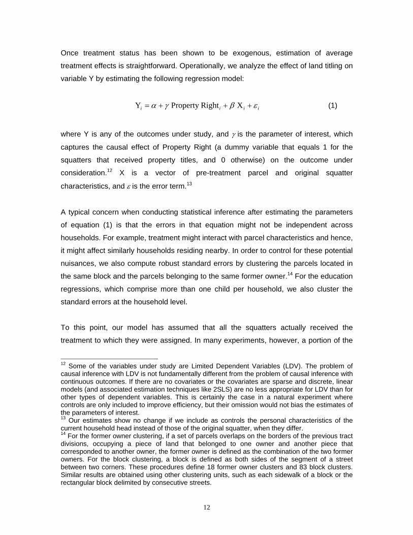
Once treatment status has been shown to be exogenous, estimation of average

treatment effects is straightforward. Operationally, we analyze the effect of land titling on

variable Y by estimating the following regression model:

iiii εβγα +++= X Right Property Y (1)

where Y is any of the outcomes under study, and γ is the parameter of interest, which

captures the causal effect of Property Right (a dummy variable that equals 1 for the

squatters that received property titles, and 0 otherwise) on the outcome under

consideration.12 X is a vector of pre-treatment parcel and original squatter

characteristics, and ε is the error term.13

A typical concern when conducting statistical inference after estimating the parameters

of equation (1) is that the errors in that equation might not be independent across

households. For example, treatment might interact with parcel characteristics and hence,

it might affect similarly households residing nearby. In order to control for these potential

nuisances, we also compute robust standard errors by clustering the parcels located in

the same block and the parcels belonging to the same former owner.14 For the education

regressions, which comprise more than one child per household, we also cluster the

standard errors at the household level.

To this point, our model has assumed that all the squatters actually received the

treatment to which they were assigned. In many experiments, however, a portion of the

12 Some of the variables under study are Limited Dependent Variables (LDV). The problem of causal inference with LDV is not fundamentally different from the problem of causal inference with continuous outcomes. If there are no covariates or the covariates are sparse and discrete, linear models (and associated estimation techniques like 2SLS) are no less appropriate for LDV than for other types of dependent variables. This is certainly the case in a natural experiment where controls are only included to improve efficiency, but their omission would not bias the estimates of the parameters of interest. 13 Our estimates show no change if we include as controls the personal characteristics of the current household head instead of those of the original squatter, when they differ. 14 For the former owner clustering, if a set of parcels overlaps on the borders of the previous tract divisions, occupying a piece of land that belonged to one owner and another piece that corresponded to another owner, the former owner is defined as the combination of the two former owners. For the block clustering, a block is defined as both sides of the segment of a street between two corners. These procedures define 18 former owner clusters and 83 block clusters. Similar results are obtained using other clustering units, such as each sidewalk of a block or the rectangular block delimited by consecutive streets.

13

participants fail to follow the treatment protocol, a problem termed treatment non-

compliance. In our case, this might be of potential concern since a number of families

that were offered the possibility of obtaining land titles did not receive them for reasons

that may also affect their outcomes. In order to address this problem of non-compliance,

we also report the reduced-form estimates from regressing the outcomes of interest on

the intention-to-treat Property Right Offer variable, a dummy indicating the availability of

land title offers, and also the 2SLS estimates of the treatment effects from instrumenting

the Property Right variable with the Property Right Offer variable.

Finally, in any investigation where the impact takes time to materialize (like the

investment, household size and long-term education achievement considered in this

paper), some participants will inevitably drop out from the analysis. For example, the

most widely used longitudinal dataset in economics, the Michigan Panel Study on

Income Dynamics, has experienced a 50 percent sample loss from cumulative attrition

after 30 years from its initial sample (see Fitzgerald et al., 1998).15 Participation attrition,

hence, is another potential problem that might bias the estimates of causal effects in

long-term studies.

In our 2003 survey, we asked each family the time of arrival to the parcel they are

currently occupying, and found that some families arrived after the (early) treatment was

assigned, i.e. after the former owners made, during 1986, the decision of surrender the

land or sue. From the sample of 467 interviewed households, we found that 313 families

had arrived to the parcel before the end of 1985, while 154 families arrived after 1985.16

As it is plausible to argue that the families that arrived after the former owners’ decisions

could have known the different expropriation status (i.e., the different probabilities of

receiving the land) associated to each parcel, in order to guarantee exogeneity we need

to exclude from the analysis the families that arrived to the parcel they are currently

occupying after 1985. Once this exclusion is made, there is basically no variability (nor

differences between treatment and control groups) in our sample in the year of arrival of

the households to the parcels they are currently occupying.

15 See also, for example, Alderman et al. (2003) and Behrman et al. (2003). 16 To identify with accuracy the time of arrival of each family to the parcel they are currently occupying, our survey asked where the original squatter was living when Diego Maradona scored the ‘Hand of God’ goal in the 1986 World Cup game against England. It is impossible for an Argentine not to remember where she/he was on that day (Amis, 2004).

14

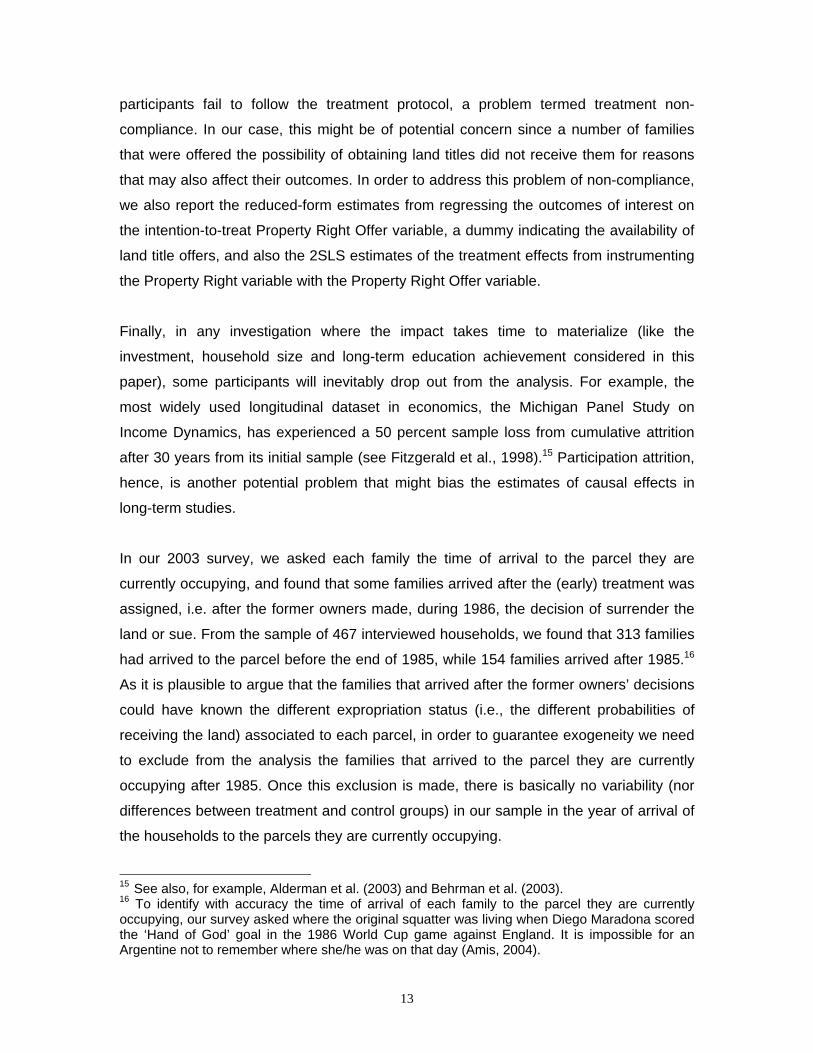
This raises, however, a problem of attrition. If some families arrived after 1985, they

could have replaced some original squatters in our treatment and control parcels that

had left before we ran our survey in 2003.17 Moreover, the availability of titles could have

affected household migration decisions. Indeed, column (1) of Table 2 shows that 62.4

percent of the parcels in the non-intention-to-treat group are inhabited by families that

arrived before 1986, while the proportion is 70.0 percent for the intention-to-treat group

in the second column.18

Table 2 – Household Attrition

Variables

Property Right

Offer=0 (1)

Property Right

Offer=1 (2)

Property Right Offer

1989=1 (3)

Property Right Offer

1998=1 (4)

Household arrived before 1986=1

0.624 (0.036)

0.700 (0.028)

0.729 (0.051)

0.689 (0.033)

Difference relative to column (1) -0.076*

(0.045) -0.105* (0.063)

-0.064 (0.049)

Notes: Standard errors are in parentheses. * Significant at 10%.

Of course, the migration decision could be potentially correlated with the outcomes

under study. We exploit two alternative strategies to address this potential nuisance. Our

first strategy takes advantage of the asynchronous timing in the titling process to

consider, separately, the early and late treatment groups. Although, relative to the

control group, the third column of Table 2 shows a significant difference in attrition for the

parcels titled in 1989 (early treatment), the last column shows no statistically significant

difference for the parcels titled in 1998 (late treatment). Moreover, the unobservable

variables that might have affected migration decisions are, a priori, more likely to be

ignorable when comparing the control and late treatment groups than when comparing

the control and early treatment groups. This is so because the squatters titled in 1998

were under the same conditions as those in the control group for 17 out of the 22 years

elapsed from the land invasion to the time of our 2003 survey, so we should expect them 17 For the families that arrived after 1985, our questionnaire attempted to collect information on the names and destination of the previous occupants of the parcels. In both treatment and control parcels, the current occupants could provide a name and/or destination of the previous occupant only for less than 20 percent of the cases. Although the information obtained is very poor, it does not suggest that the households that left the untitled parcels moved to richer areas than the families that left the titled parcels.

15

to have broadly similar experiences. Indeed, most of the out-migration for these two

groups occurred during the interim period they were both untitled. The survival rates for

the late titled and control groups since 1997 (i.e., just before the late treated received

titles) are 0.958 (s.e. 0.014) and 0.939 (s.e. 0.017), respectively. Thus, the estimated

effects of land titling for the late titled group are unlikely to be biased by attrition.

Additionally, the comparison of these coefficients with those corresponding to the

estimated effects of land titling for the early treated group leads to an indirect test of

whether attrition in the latter group is also ignorable.

A more standard strategy assumes the data are missing at random conditional on

observable characteristics. The idea is then to compare the outcomes for treated and

control survivors with similar pre-treatment characteristics. This approach leads to

matching methods based on the propensity score of sample selection. The validity of this

strategy requires that at least one of the pre-treatment characteristics predicts attrition.

The only pre-treatment characteristics available for the whole set of squatters (attrited

and non-attrited) are the parcel characteristics reported in Panel A of Table 1. We

estimate a Logit model of the likelihood of survival since 1985 on these parcel

characteristics, and find that the distance to the nearby polluted and floodable creek has

a positive and statistically significant effect on this likelihood. We exploit the variability in

attrition induced by this pre-treatment characteristic to correct for sample selection.

We implement the matching selection correction by means of the method of stratification

matching. First, we eliminate observations outside the common support of the estimated

propensity score for the distributions of titled and untitled groups. Second, we divide the

range of variation of the propensity score in intervals such that within each interval,

treated and control units have on average the same propensity score. Third, within each

interval, the difference between the average outcomes of the treated and the controls is

computed. The parameter of interest is finally obtained as an average of the estimates of

each interval weighted by the share of treated units in each interval on all treated units.

18 These survival rates could be overestimating attrition by assuming that there were no vacated parcels left after the occupation.

16

V. Results In this section we investigate the causal effect on housing investment, household

structure, human capital accumulation, access to credit, and labor earnings, of providing

squatters with formal titles of the parcels of land they occupy. This is the treatment of

interest in policy analysis in the developing world, where most interventions consist of

titling occupied tracts of land to the current inhabitants.19

Ownership of property gives its owner multiple rights. In its most complete form, they

include the rights to use the asset, to exclude others from using it, to transfer the assets

to others, and to persist in these rights (Barzel, 1997). In our natural experiment, the

entitled households acquired full property rights (with the only restriction that the parcels

cannot be legally transferred for the first ten years after titling). The untitled households,

instead, are still living in the occupied parcels without paying rent and property taxes, but

they are uncertain about when and if the parcels will be titled. Moreover, the untitled may

feel uncertain about which member of the household would receive the title, and they

may fear the occupation of their parcels by new squatters before titling. In the meantime,

the untitled cannot legally transfer their usufructuary rights.

V.1. Effects on Housing Investment

The possession of land titles may affect the incentives to invest in housing construction

through several concurrent mechanisms. The traditional view emphasizes security from

seizure. Individuals underinvest if others may seize the fruits of their investments. Land

titles can also encourage investment by improving the transferability of the parcels. Even

if there were no risk of expropriation, investments in untitled parcels would be highly

illiquid, whereas titling reduces the cost of alienation of the assets. A third mechanism is

through the credit market. Transferability might allow the use of the land as collateral,

diminishing the funding constraints on investment. Finally, a fourth link is that land titles

19 Whether the provision of land titles to squatters in this area could have encouraged new squatting (and therefore, violation of landowners’ property rights) in other zones is beyond the scope of our study, but should not be ignored in the evaluation of the overall impact of this type of interventions.

17

provide poor households with a valuable savings tool. Poor households, especially in

unstable macroeconomic environments, lack appropriate savings instruments. Land titles

allow households to substitute present consumption and leisure into long-term savings in

real property. We now investigate empirically the impact of legal land titles on housing

investment.

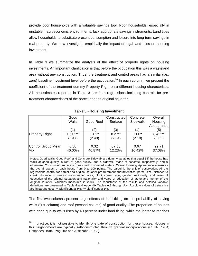
In Table 3 we summarize the analysis of the effect of property rights on housing

investments. An important clarification is that before the occupation this was a wasteland

area without any construction. Thus, the treatment and control areas had a similar (i.e.,

zero) baseline investment level before the occupation.20 In each column, we present the

coefficient of the treatment dummy Property Right on a different housing characteristic.

All the estimates reported in Table 3 are from regressions including controls for pre-

treatment characteristics of the parcel and the original squatter.

Table 3 - Housing Investment

Good Walls

(1)

Good Roof

(2)

Constructed Surface

(3)

Concrete Sidewalk

(4)

Overall Housing

Appearance(5)

Property Right 0.20*** 0.15** 8.27** 0.11** 8.42*** (3.47) (2.49) (2.34) (2.18) (3.65) Control Group Mean 0.50 0.32 67.63 0.67 22.71 %∆ 40.00% 46.87% 12.23% 16.42% 37.08% Notes: Good Walls, Good Roof, and Concrete Sidewalk are dummy variables that equal 1 if the house has walls of good quality, a roof of good quality, and a sidewalk made of concrete, respectively, and 0 otherwise. Constructed surface is measured in squared meters. Overall Housing Appearance measures the overall aspect of each house from 0 to 100 points. The parcel is the unit of observation. All the regressions control for parcel and original squatter pre-treatment characteristics: parcel size; distance to creek; distance to nearest non-squatted area; block corner; age, gender, nationality, and years of education of the original squatter; and nationality and years of education of father and mother of the original squatter. Variables measured in 2003. The robustness of the results and detailed variable definitions are presented in Table 4 and Appendix Tables A.1 through A.4. Absolute values of t statistics are in parentheses. ** Significant at 5%; *** significant at 1%.

The first two columns present large effects of land titling on the probability of having

walls (first column) and roof (second column) of good quality. The proportion of houses

with good quality walls rises by 40 percent under land titling, while the increase reaches

20 In practice, it is not possible to identify one date of construction for these houses. Houses in this neighborhood are typically self-constructed through gradual incorporations (CEUR, 1984; Cespedes, 1984; Izaguirre and Aristizabal, 1988).

18

47 percent for good quality roof. The third column presents the effect of land titling on

the total surface constructed in the parcel. Our results suggest a statistically significant

increase of about 12 percent in constructed surface under the presence of land titles.

The fourth column shows a statistically significant increase of 16 percent in the

proportion of houses with sidewalks made of concrete. In the last column, the variable

Overall Housing Appearance summarizes the overall aspect of each house using an

index from 0 to 100 points assigned by the team of architects. The coefficient shows a

large and significant effect of land titling on housing quality. Relative to the baseline

average sample value, the estimated effect represents an overall housing improvement

of 37 percent associated to titling.

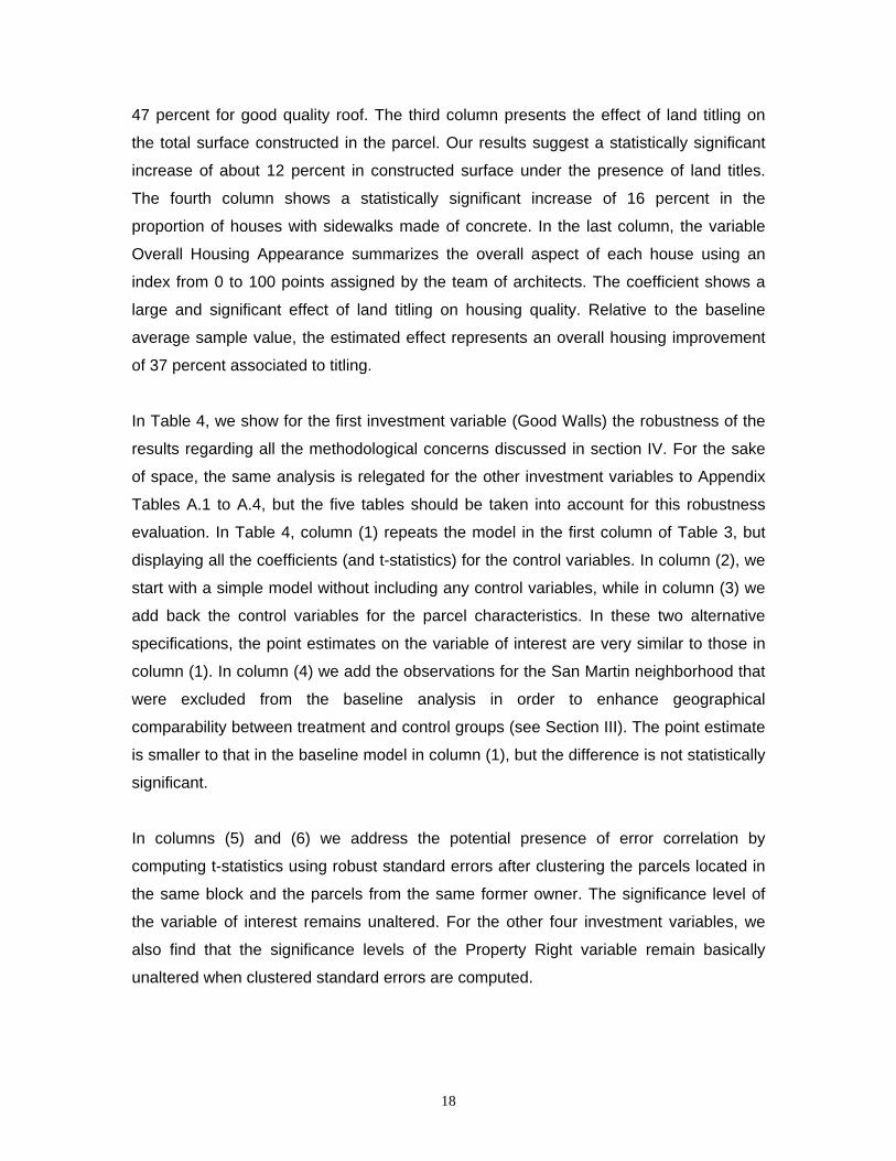
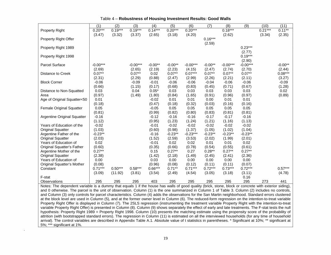
In Table 4, we show for the first investment variable (Good Walls) the robustness of the

results regarding all the methodological concerns discussed in section IV. For the sake

of space, the same analysis is relegated for the other investment variables to Appendix

Tables A.1 to A.4, but the five tables should be taken into account for this robustness

evaluation. In Table 4, column (1) repeats the model in the first column of Table 3, but

displaying all the coefficients (and t-statistics) for the control variables. In column (2), we

start with a simple model without including any control variables, while in column (3) we

add back the control variables for the parcel characteristics. In these two alternative

specifications, the point estimates on the variable of interest are very similar to those in

column (1). In column (4) we add the observations for the San Martin neighborhood that

were excluded from the baseline analysis in order to enhance geographical

comparability between treatment and control groups (see Section III). The point estimate

is smaller to that in the baseline model in column (1), but the difference is not statistically

significant.

In columns (5) and (6) we address the potential presence of error correlation by

computing t-statistics using robust standard errors after clustering the parcels located in

the same block and the parcels from the same former owner. The significance level of

the variable of interest remains unaltered. For the other four investment variables, we

also find that the significance levels of the Property Right variable remain basically

unaltered when clustered standard errors are computed.

19

Table 4 – Robustness of Housing Investment Results: Good Walls

(1) (2) (3) (4) (5) (6) (7) (8) (9) (10) (11) Property Right 0.20*** 0.19*** 0.19*** 0.14*** 0.20*** 0.20*** 0.18*** 0.21*** 0.11** (3.47) (3.32) (3.37) (2.65) (3.18) (4.20) (2.62) (3.34) (2.35) Property Right Offer 0.16*** (2.59) Property Right 1989 0.23*** (2.77) Property Right 1998 0.19*** (2.90) Parcel Surface -0.00*** -0.00*** -0.00** -0.00** -0.00*** -0.00** -0.00*** -0.00*** -0.00** (2.69) (2.65) (2.19) (2.23) (4.15) (2.47) (2.74) (2.70) (2.44) Distance to Creek 0.07** 0.07** 0.02 0.07** 0.07*** 0.07** 0.07** 0.07** 0.08*** (2.31) (2.29) (0.88) (2.47) (2.99) (2.26) (2.21) (2.11) (3.27) Block Corner -0.06 -0.09 -0.01 -0.06 -0.06 -0.04 -0.06 -0.06 -0.09 (0.66) (1.15) (0.17) (0.68) (0.83) (0.45) (0.71) (0.67) (1.28) Distance to Non-Squatted 0.03 0.04 0.05* 0.03 0.03 0.03 0.03 0.03 0.02 Area (0.97) (1.49) (1.80) (0.84) (1.65) (0.91) (0.96) (0.97) (0.89) Age of Original Squatter<50 0.01 -0.02 0.01 0.01 0.00 0.01 0.01 (0.18) (0.47) (0.18) (0.32) (0.03) (0.16) (0.16) Female Original Squatter 0.05 -0.05 0.05 0.05 0.05 0.05 0.05 (0.81) (0.99) (0.82) (0.80) (0.83) (0.81) (0.81) Argentine Original Squatter -0.16 -0.12 -0.16 -0.16 -0.17 -0.17 -0.16 (1.12) (0.95) (1.23) (1.24) (1.21) (1.16) (1.13) Years of Education of the -0.02 -0.01 -0.02 -0.02 -0.02 -0.02 -0.02 Original Squatter (1.03) (0.60) (0.98) (1.37) (1.05) (1.02) (1.04) Argentine Father of the -0.23** -0.16 -0.23** -0.23*** -0.23** -0.23** -0.23** Original Squatter (2.03) (1.52) (2.59) (3.53) (2.02) (1.99) (2.01) Years of Education of 0.02 -0.01 0.02 0.02 0.01 0.01 0.02 Original Squatter’s Father (0.60) (0.35) (0.66) (0.78) (0.54) (0.55) (0.61) Argentine Mother of the 0.27** 0.15 0.27** 0.27 0.28** 0.27** 0.27** Original Squatter (2.38) (1.42) (2.18) (1.49) (2.45) (2.41) (2.36) Years of Education of 0.00 0.03 0.00 0.00 0.00 0.00 0.00 Original Squatter’s Mother (0.08) (0.96) (0.08) (0.12) (0.11) (0.11) (0.07) Constant 0.71*** 0.50*** 0.58*** 0.66*** 0.71** 0.71*** 0.72*** 0.73*** 0.72*** 0.57*** (3.09) (11.92) (3.81) (3.54) (2.49) (4.54) (3.05) (3.18) (3.11) (4.78) F-stat 0.16 Observations 295 295 295 403 295 295 295 295 295 273 441 Notes: The dependent variable is a dummy that equals 1 if the house has walls of good quality (brick, stone, block or concrete with exterior siding), and 0 otherwise. The parcel is the unit of observation. Column (1) is the one summarized in Column 1 of Table 3. Column (2) includes no controls, and Column (3) only controls for parcel characteristics. Column (4) adds the observations for the San Martin neighborhood. Standard errors clustered at the block level are used in Column (5), and at the former owner level in Column (6). The reduced-form regression on the intention-to-treat variable Property Right Offer is displayed in Column (7). The 2SLS regression (instrumenting the treatment variable Property Right with the intention-to-treat variable Property Right Offer) is presented in Column (8). Column (9) shows separately the effect of early and late treatments. The F-stat tests the null hypothesis: Property Right 1989 = Property Right 1998. Column (10) presents the matching estimate using the propensity score of the probability of attrition (with bootstrapped standard errors). The regression in Column (11) is estimated on all the interviewed households (for any time of household arrival). The control variables are described in Appendix Table A.1. Absolute value of t statistics in parentheses. * Significant at 10%; ** significant at 5%; *** significant at 1%.

.

20

Columns (7) and (8) deal with the potential problem of non-compliance. In column (7) we

estimate the reduced-form parameter on the intention-to-treat Property Right Offer

variable, while in column (8) we report the 2SLS estimates of instrumenting the Property

Right variable with Property Right Offer. For the five investment variables, both

estimates are very similar to those obtained from OLS in the baseline specification and

the differences are not statistically significant at conventional levels, suggesting that non-

compliance is not an issue of concern in our sample.21

In Columns (9) and (10) we address the concern that these results might be generated

by attrition in the original squatter population and are not the cause of treatment. In

Column (9) we separately report the effects for early and late land titling, exploiting the

fact that, as shown in Table 2, the attrition rates of the late-treated and control groups

are not significantly different. The results show that both the early and late treatments

have positive significant effects on Good Walls and the other investment variables. For

all the variables, the point estimates for the late treatment coefficient are very similar to

the ones in the baseline specification in column (1). Moreover, the F-statistics show that

we cannot reject the null hypotheses that the effects for the early-treated group and late-

treated group are similar at conventional levels of significance.22 Column (10) reports the

matching estimates discussed in the previous section. Again, for Good Walls and the

other investment variables, the point estimates are quite similar to those in the baseline

specification and the differences are never statistically significant. Thus, the evidence

suggests that the estimates in Table 3 identify the causal effect of land titling on

investment and not a statistical artifact due to attrition.

Finally, in column (11) we consider the whole sample of 448 parcels where households

were interviewed, instead of considering only the parcels occupied by households that

arrived before the time the former owners decided to surrender the land or sue. This

analysis investigates a different parameter than the one considered so far. The

21 The first-stage regression of Property Right on Property Right Offer is very strong. For the households that arrived before 1986 (i.e. the non-attrited group) and live in parcels offered for titling, the non-compliance rate is 11.2% (9.3% for the early treated, and 12% for the late treated). 22 If one was still to worry about the possibility that the former owners’ decisions of accepting or disputing the government offer was correlated with land or squatter characteristics, the significance of the late-treatment coefficients and their similarity with the early-treatment ones should be reassuring. In both the late-treated and control areas, the squatters settled on eventually contested tracts of land and are, therefore, homogenous regarding the decisions of their respective original owners (see section II).

21

estimated coefficient measures the causal effect of securing property rights on

investment in a given parcel regardless of whether the family occupying it could have

changed over time.23 The estimated coefficients for the different investment variables are

sometimes smaller but, overall, of similar magnitude to those in the baseline models.

A final question relates to the interpretation of the identified causal effect of land titling on

investment. Is this an incentive effect induced by owning formal property rights, or is it

mainly a wealth effect from titled households that became richer, housing being a normal

good? The evidence suggests the treatment operates by affecting the incentives to

invest. First, the size of the differential wealth transfer was moderate (see footnote 3)

and seems considerably smaller than the value of the constructed dwellings.24 Second,

the families could not have financed the investments with the wealth transfer. It would be

impossible to sell the land and, at the same time, invest the collected money on it.

Moreover, access to credit improved little with titling (see section V.4). Third, Appendix

Table 5 shows no differences in the consumption of durable goods (refrigerators,

freezers, washing machines, TV sets and cellular phones). This suggests that the large

investment effects presented in this section are a result of a change in the economic

returns to housing investment induced by the land titles, and not just a response to a

wealth effect that should have also affected the consumption of these goods.25

We conclude that moving a poor household from usufructuary rights to full property

rights substantially improves housing quality. The estimated effects are large and robust,

and seem to be the result of changes in the economic returns to housing investment

induced by land titling. Thus, our micro evidence supports the hypothesis that securing

property rights significantly increases investment levels.

23 In these regressions that ignore household rotation, the estimated coefficient can be interpreted as “what grows in a parcel when it is entitled” regardless of whether the same family has always been occupying it or has been replaced by another one. Instead, the estimates obtained exclusively on the non-attrited households measure “what a given family builds in a parcel when receives a land title”. 24 For areas of this level of development in the Buenos Aires outskirts, Zavalia Lagos (2005) estimates that the values of the constructed houses exceed the parcel values by five times. 25 There are no differences in the access to public services. Basically all the households (titled and untitled) have connections to the water and electricity networks, whereas there are no sewage and natural gas networks in the area.

22

V.2. Effects on Household Size

The possession of land titles may also affect the size and structure of households. There

are several potential reasons for that to happen. Insurance motives seem to be the most

important. The poor lack access to well-functioning insurance markets and pension

systems that could protect them during bad times and retirement. With limited access to

risk diversification, to savings instruments, and to the social security system, the need for

insurance has to be satisfied by other means. A traditional provider of insurance among

the poor is the extended family. Another possibility is to use children as future insurance.

In particular, old-age security motives can induce higher fertility (see, among others,

Cain, 1985, Nugent, 1985, Ray, 1997, and Portner, 2001).26 By allowing the use of

housing investment as a savings tool, by securing shelter for the old age, and by

potentially improving credit access, land titling may provide some of the needed

insurance, therefore reducing the demand for household members among the titled

group.27

Moreover, the lack of land titles might reduce the ability of household heads to restrict

their relatives from residing in their houses. The household heads may feel less powerful

to expel or to deny access to members of their extended family when they lack formal

titles. The lack of titles may also impede the division of wealth among family members,

forcing claimants to live together to enjoy and retain usufructuary rights. For example,

siblings (with their spouses and children) may end up having to live together if they

cannot divide their inheritance upon the death of their untitled parents. In addition,

untitled households may feel in need of increasing the number of family members in

order to protect their houses from occupation by other squatters (Lanjouw and Levy,

26 “[An] important question is whether having many children and/or a large extended household is an optimizing strategy allowing households to derive benefits otherwise lost due to poorly functioning markets” (Birdsall 1988, pp. 502). 27 David and Sundstrom (1984) explain the fertility changes in US history using a similar argument. Suppose, they argue, that large families were designed to be old-age insurance for the parents. At the time of independence, the superabundance of arable land meant that the price of land would not rise over time sufficiently to be a nest egg for old age, and children would be needed to care for their aged parents. When, late in the nineteenth century, the best lands were growing scarce, then the rent, and therefore the price, of land already owned and settled would increase becoming a nest egg due to its capital gain. Thus, investment in land operated as a substitute for more children. The scarcer the land, the higher the economic rent and capital gain, and the fewer children needed to provide for the declining years of the parents.

23

2002; Field, 2007). Through these concurrent mechanisms, the lack of formal land titles

may generate, on average, larger households among the untitled group.

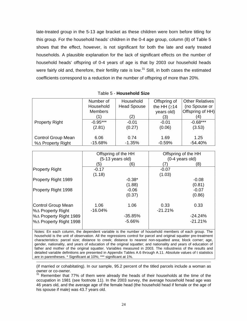
In Table 5, we find large differences in household size between titled and untitled

families. Untitled families have an average of 6.06 members, while titled households

have 0.95 members less. Table 5 also shows that the difference in household size does

not originate in a more frequent presence in the control group of a spouse of the

household head (column 2), nor of offspring of the household head older than 13 years

old, i.e. born before the first land titles were issued (column 3). This last result is

important, because it suggests that there were no differences in the number of children

of the household head born before treatment.28

The difference in household size seems to originate in two factors. First, column (4) of

Table 5 shows a higher presence (0.68 members) of non-nuclear relatives in untitled

households. Untitled households report a much larger number of further relatives of the

household head who are not her/his spouse or offspring (i.e., siblings, parents, in-laws,

grandchildren, etc.) than entitled households.29

Second, the entitled households show a smaller number of offspring of the household

head born after the title allocation. To better analyze this result, we split the household

heads’ offspring into those born between the first and the second title allocation (children

between 5 and 13 years old), and those born after the second title allocation (children

between 0 and 4 years old). For the 5-13 age group, column (6) of Table 5 shows a

significant reduction of 36% in the number of household heads’ children for the early-

treated households. This decrease corresponds to 8.5% of the sample average of total

household heads’ offspring.30 The effect, instead, is not significant for the late-treated

group. This result is reassuring, since treatment could not have affected fertility for the 28 The regression in column (3) only considers offspring living in the house. Non-significant differences are also obtained for the total number of household head’s offspring older than 13 (i.e., living and not living in the parental home). 29 The hypothesis that extended family members are valuable to protect the house from other squatters would suggest a larger share of males among non-nuclear adult members in the control group than in the treatment group. In our dataset, however, the male proportion of non-nuclear adults is actually smaller in the control group. 30 This fertility effect does not depend on whether a woman or a man received the title. According to the expropriation law, the titles were awarded to both the household head and her/his spouse

24

late-treated group in the 5-13 age bracket as these children were born before titling for

this group. For the household heads’ children in the 0-4 age group, column (8) of Table 5

shows that the effect, however, is not significant for both the late and early treated

households. A plausible explanation for the lack of significant effects on the number of

household heads’ offspring of 0-4 years of age is that by 2003 our household heads

were fairly old and, therefore, their fertility rate is low.31 Still, in both cases the estimated

coefficients correspond to a reduction in the number of offspring of more than 20%.

Table 5 - Household Size

Number of Household Members

(1)

Household Head Spouse

(2)

Offspring of the HH (≥14 years old)

(3)

Other Relatives (no Spouse or

Offspring of HH)(4)

Property Right -0.95*** -0.01 -0.01 -0.68*** (2.81) (0.27) (0.06) (3.53) Control Group Mean 6.06 0.74 1.69 1.25 %∆ Property Right -15.68% -1.35% -0.59% -54.40%

Offspring of the HH (5-13 years old)

Offspring of the HH (0-4 years old)

(5) (6) (7) (8) Property Right -0.17 -0.07 (1.18) (1.03) Property Right 1989 -0.38* -0.08 (1.88) (0.81) Property Right 1998 -0.06 -0.07 (0.37) (0.86) Control Group Mean 1.06 1.06 0.33 0.33 %∆ Property Right -16.04% -21.21% %∆ Property Right 1989 -35.85% -24.24% %∆ Property Right 1998 -5.66% -21.21% Notes: En each column, the dependent variable is the number of household members of each group. The household is the unit of observation. All the regressions control for parcel and original squatter pre-treatment characteristics: parcel size; distance to creek; distance to nearest non-squatted area; block corner; age, gender, nationality, and years of education of the original squatter; and nationality and years of education of father and mother of the original squatter. Variables measured in 2003. The robustness of the results and detailed variable definitions are presented in Appendix Tables A.6 through A.11. Absolute values of t statistics are in parentheses. * Significant at 10%; *** significant at 1%. (if married or cohabitating). In our sample, 95.2 percent of the titled parcels include a woman as owner or co-owner. 31 Remember that 77% of them were already the heads of their households at the time of the occupation in 1981 (see footnote 11). In the 2003 survey, the average household head age was 46 years old, and the average age of the female head (the household head if female or the age of his spouse if male) was 43.7 years old.

25

The robustness of these results regarding the methodological concerns discussed in

section IV is presented in Appendix Tables A.6 to A.11.32 Moreover, the results are

robust to controlling for whether the original squatter is the current household head, for

the age of the household head, and, in the regressions for the household heads’ children

of 5-13 and 0-4 years of age, for the number of offspring of the household head

previously born. In summary, we find that entitled households are smaller than untitled

ones. The larger size of households in the untitled parcels is due to both a larger number

of offspring of the household head and a more frequent presence of non-nuclear

relatives.

V.3. Effects on Educational Achievement

The seminal work of Becker and Lewis (1973) advanced the presence of parental trade-

offs between the quantity and the quality of children. This trade-off appears because

limited parents’ time and resources are spread over more children (see Rosenzweig and

Wolpin (1980), Hanushek (1992), and Li et al. (2008) for empirical evidence). If land

titling causes a reduction in fertility, it could also induce households to increase

educational investments in their children. Moreover, land titling could also have

beneficial effects on the education of household heads’ offspring through the reduction in

the number of extended family members living in the house and the potential health

consequences of improved housing (Goux and Maurin, 2005).

We explore this hypothesis by looking at differences in educational outcomes. In Table 8

we first consider the School Achievement variable, which is the difference between the

school grade the child is currently attending or the maximum grade attained (if she/he is

not currently attending school) minus the grade corresponding to her/his age. This

variable measures the performance of children from primary school on, collapsing

differences in school dropout, grade repetition, and age of school initiation. We consider

children from 6 years of age (the beginning of primary school) to 20 years of age at the

time of the 2007 survey.33 For the offspring of the household head in the early-treated

32 For those results that should only be present for the early-treated group, we cannot test the robustness of our results by contrasting the effects for the early and late groups. In these cases, we use only the matching estimates as robustness tests to address the attrition concern. 33 Our approach is similar to the one used in the literature that uses twin births to study the effect of the number of children in the household on children education. The children born before

26

households (the households for which in column (6) of Table 5 we found a reduction in

the number of members), column (2) of Table 6 shows a large effect on School

Achievement. The children in the control group show an average delay of 1.95 years in

their school achievement, whereas this delay is 0.69 years shorter for the children in the

early-titled parcels. The effect is not significant for the children in the late-treated

households, which had not shown a fertility reduction.34

In columns (3) and (4), we compare differences in primary school completion. Primary

school is mandatory in Argentina and compliance is high, particularly in urban areas. We

find no differences in this variable. Children from both titled and untitled households

show primary school graduation rates above 80%. Thus, most of the delay in school

achievement occurs after primary school. For the children in primary school age (6 to 12

years of age) the School Achievement variable takes an average of -0.32 for the control

group, with no significant differences relative to the early or late treated groups.

“treatment” (i.e., before the nth delivery for which some families in the sample have twins) are also included in the analysis. 34 The regressions in Table 6 are estimated at the child level and include controls for child age and gender. In addition to clustering the standard errors at the block and former owner levels,

27

Table 6 – Education

Offspring of the Household Head

School Achievement (6-20 years old)

Primary School Completion (13-20 years old)

(1) (2) (3) (4) Property Right 0.23 0.02 (1.21) (0.47) Property Right 1989 0.69** 0.02 (2.30) (0.34) Property Right 1998 0.04 0.02 (0.20) (0.40) Control Group Mean -1.95 -1.95 0.80 0.80

Secondary School Completion(18-20 years old)

Post-Secondary Education (18-20 years old)

(5) (6) (7) (8) Property Right 0.06 0.10* (0.80) (1.94) Property Right 1989 0.28** 0.20** (2.05) (2.30) Property Right 1998 -0.00 0.07 (0.07) (1.20) Control Group Mean 0.25 0.25 0.04 0.04 Notes: In columns (1) and (2), the dependent variable is the difference between the school grade each child is currently attending or the maximum grade attained (if not attending school) minus the grade corresponding to the child age. In columns (3) and (4), the dependent variable is a dummy that equals 1 if the child has finished primary school, and 0 otherwise. In columns (5) and (6), the dependent variable is a dummy that equals 1 if the child has finished secondary school, and 0 otherwise. In columns (7) and (8), the dependent variable is a dummy that equals 1 if the child has started post-secondary education (tertiary or university), and 0 otherwise. The child is the unit of observation. All the regressions control for child age, child gender, and parcel and original squatter pre-treatment characteristics (parcel size; distance to creek; distance to nearest non-squatted area; block corner; age, gender, nationality, and years of education of the original squatter; and nationality and years of education of original squatter’s parents). Education variables measured in 2007. The robustness of the results and detailed variable definitions are presented in Appendix Tables A.12 through A.15. Absolute values of t statistics are in parentheses. * Significant at 10%; ** significant at 5%.

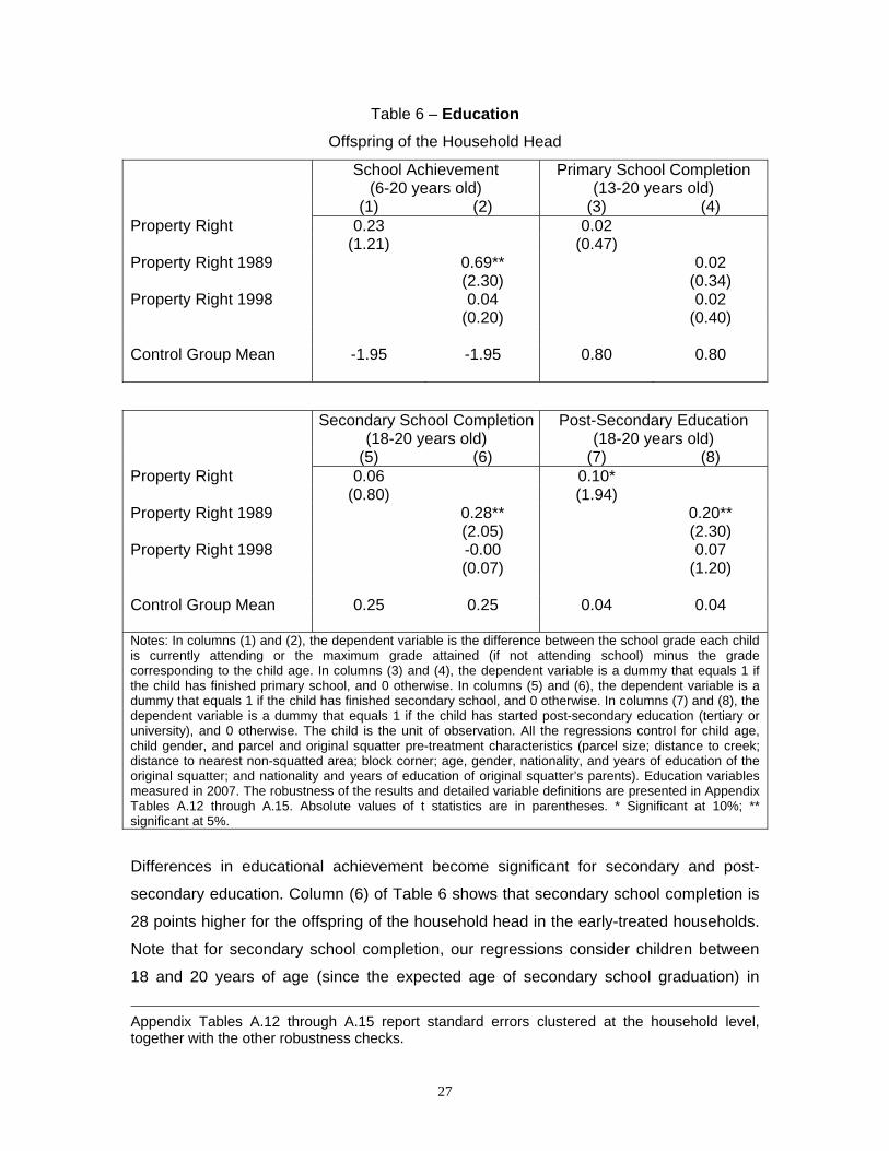
Differences in educational achievement become significant for secondary and post-

secondary education. Column (6) of Table 6 shows that secondary school completion is

28 points higher for the offspring of the household head in the early-treated households.

Note that for secondary school completion, our regressions consider children between

18 and 20 years of age (since the expected age of secondary school graduation) in

Appendix Tables A.12 through A.15 report standard errors clustered at the household level, together with the other robustness checks.

28

2007. In the early-titled parcels, these children were born just before treatment. Thus,

the effect is only significant for the group of children who were raised in families with a

small number of siblings thanks to, according to the estimates in the previous section,

the reduction in fertility their parents experienced after titling. Similar results are

presented in column (8), which shows that continuation into tertiary or university

education is 20 points higher for children in the early-treated households, again the ones

that showed the fertility reduction.

How large is the effect of land titling on school achievement? Consider, for example, the

successful Mexican anti-poverty program Progresa, which provides monetary transfers

to families that are contingent upon their children’s regular school attendance. The

estimates in Behrman et al. (2005) indicate that if children were to participate in the

program between their 6 to 14 years of age, they would experience an increase of 0.6

years in average educational attainment levels, an effect comparable to the one we

estimate for land titling in column (2) of Table 6. In addition, in a standard Mincer

earnings equation using wage data from the official Argentine household survey (EPH,

2006), the returns to secondary school completion and incomplete tertiary education are

estimated to be approximately 20% and 40%, respectively, above those for incomplete

secondary school. These large wage differentials augur significant long-term effects on

the future labor market returns of the squatters’ offspring.

V.4. Effects on Performance in the Credit and Labor Markets

Financial markets in developing countries are highly imperfect and these imperfections

are particularly severe for the poor. The possession of formal property rights could allow

the use of land as collateral, improving the access of the poor to the credit markets

(Feder et al., 1988). In turn, this collateralized credit could be invested as capital,

increasing labor productivity and income (De Soto, 2000). Moreover, land titling may

have direct labor market effects if it relieves families from the need of leaving adults at

home to protect their houses from occupation by other squatters (Field, 2007). We

investigate whether land titles improve the performance of households in the credit and

labor markets.

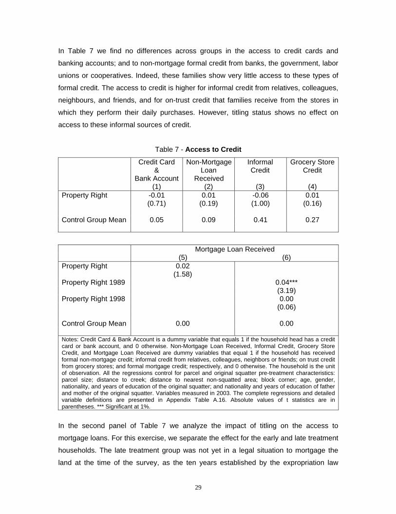
29

In Table 7 we find no differences across groups in the access to credit cards and

banking accounts; and to non-mortgage formal credit from banks, the government, labor

unions or cooperatives. Indeed, these families show very little access to these types of

formal credit. The access to credit is higher for informal credit from relatives, colleagues,

neighbours, and friends, and for on-trust credit that families receive from the stores in

which they perform their daily purchases. However, titling status shows no effect on

access to these informal sources of credit.

Table 7 - Access to Credit

Credit Card &

Bank Account (1)

Non-Mortgage Loan

Received (2)

Informal Credit

(3)

Grocery Store Credit

(4)

Property Right -0.01 0.01 -0.06 0.01 (0.71) (0.19) (1.00) (0.16) Control Group Mean 0.05 0.09 0.41 0.27

Mortgage Loan Received (5) (6)

Property Right 0.02 (1.58) Property Right 1989 0.04*** (3.19) Property Right 1998 0.00 (0.06) Control Group Mean 0.00 0.00 Notes: Credit Card & Bank Account is a dummy variable that equals 1 if the household head has a credit card or bank account, and 0 otherwise. Non-Mortgage Loan Received, Informal Credit, Grocery Store Credit, and Mortgage Loan Received are dummy variables that equal 1 if the household has received formal non-mortgage credit; informal credit from relatives, colleagues, neighbors or friends; on trust credit from grocery stores; and formal mortgage credit; respectively, and 0 otherwise. The household is the unit of observation. All the regressions control for parcel and original squatter pre-treatment characteristics: parcel size; distance to creek; distance to nearest non-squatted area; block corner; age, gender, nationality, and years of education of the original squatter; and nationality and years of education of father and mother of the original squatter. Variables measured in 2003. The complete regressions and detailed variable definitions are presented in Appendix Table A.16. Absolute values of t statistics are in parentheses. *** Significant at 1%.

In the second panel of Table 7 we analyze the impact of titling on the access to

mortgage loans. For this exercise, we separate the effect for the early and late treatment

households. The late treatment group was not yet in a legal situation to mortgage the

land at the time of the survey, as the ten years established by the expropriation law

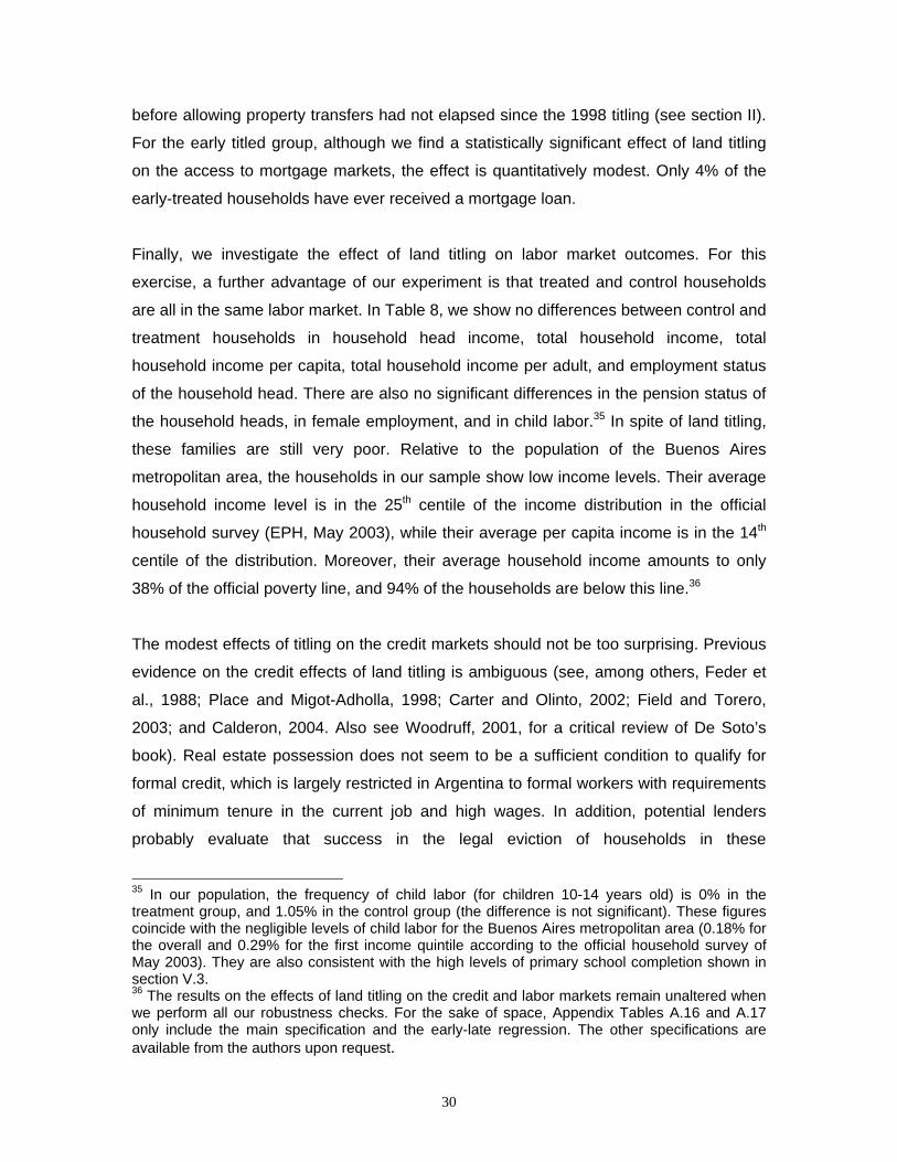
30

before allowing property transfers had not elapsed since the 1998 titling (see section II).

For the early titled group, although we find a statistically significant effect of land titling

on the access to mortgage markets, the effect is quantitatively modest. Only 4% of the

early-treated households have ever received a mortgage loan.

Finally, we investigate the effect of land titling on labor market outcomes. For this

exercise, a further advantage of our experiment is that treated and control households

are all in the same labor market. In Table 8, we show no differences between control and

treatment households in household head income, total household income, total

household income per capita, total household income per adult, and employment status

of the household head. There are also no significant differences in the pension status of

the household heads, in female employment, and in child labor.35 In spite of land titling,

these families are still very poor. Relative to the population of the Buenos Aires

metropolitan area, the households in our sample show low income levels. Their average

household income level is in the 25th centile of the income distribution in the official

household survey (EPH, May 2003), while their average per capita income is in the 14th

centile of the distribution. Moreover, their average household income amounts to only

38% of the official poverty line, and 94% of the households are below this line.36

The modest effects of titling on the credit markets should not be too surprising. Previous

evidence on the credit effects of land titling is ambiguous (see, among others, Feder et

al., 1988; Place and Migot-Adholla, 1998; Carter and Olinto, 2002; Field and Torero,

2003; and Calderon, 2004. Also see Woodruff, 2001, for a critical review of De Soto’s

book). Real estate possession does not seem to be a sufficient condition to qualify for

formal credit, which is largely restricted in Argentina to formal workers with requirements

of minimum tenure in the current job and high wages. In addition, potential lenders

probably evaluate that success in the legal eviction of households in these

35 In our population, the frequency of child labor (for children 10-14 years old) is 0% in the treatment group, and 1.05% in the control group (the difference is not significant). These figures coincide with the negligible levels of child labor for the Buenos Aires metropolitan area (0.18% for the overall and 0.29% for the first income quintile according to the official household survey of May 2003). They are also consistent with the high levels of primary school completion shown in section V.3. 36 The results on the effects of land titling on the credit and labor markets remain unaltered when we perform all our robustness checks. For the sake of space, Appendix Tables A.16 and A.17 only include the main specification and the early-late regression. The other specifications are available from the authors upon request.

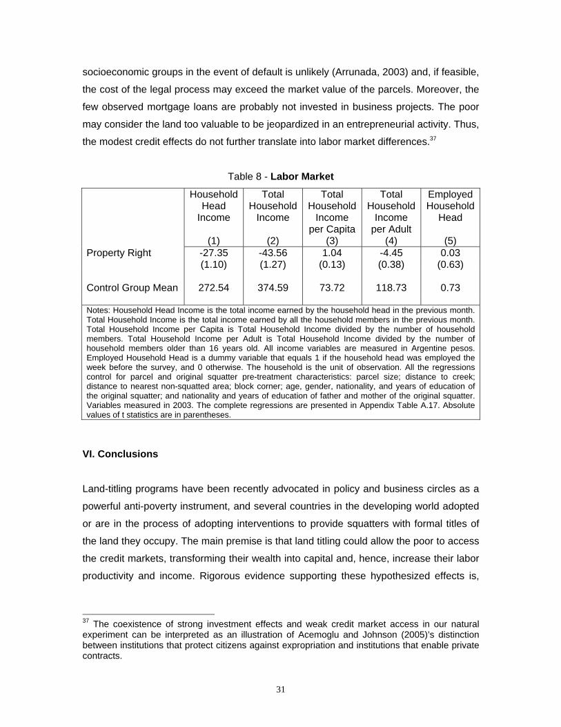
31

socioeconomic groups in the event of default is unlikely (Arrunada, 2003) and, if feasible,

the cost of the legal process may exceed the market value of the parcels. Moreover, the

few observed mortgage loans are probably not invested in business projects. The poor

may consider the land too valuable to be jeopardized in an entrepreneurial activity. Thus,

the modest credit effects do not further translate into labor market differences.37

Table 8 - Labor Market

Household Head

Income

(1)

Total Household

Income

(2)

Total Household

Income per Capita

(3)

Total Household

Income per Adult

(4)

Employed Household

Head

(5) Property Right -27.35 -43.56 1.04 -4.45 0.03 (1.10) (1.27) (0.13) (0.38) (0.63) Control Group Mean 272.54 374.59 73.72 118.73 0.73 Notes: Household Head Income is the total income earned by the household head in the previous month. Total Household Income is the total income earned by all the household members in the previous month. Total Household Income per Capita is Total Household Income divided by the number of household members. Total Household Income per Adult is Total Household Income divided by the number of household members older than 16 years old. All income variables are measured in Argentine pesos. Employed Household Head is a dummy variable that equals 1 if the household head was employed the week before the survey, and 0 otherwise. The household is the unit of observation. All the regressions control for parcel and original squatter pre-treatment characteristics: parcel size; distance to creek; distance to nearest non-squatted area; block corner; age, gender, nationality, and years of education of the original squatter; and nationality and years of education of father and mother of the original squatter. Variables measured in 2003. The complete regressions are presented in Appendix Table A.17. Absolute values of t statistics are in parentheses.

VI. Conclusions

Land-titling programs have been recently advocated in policy and business circles as a

powerful anti-poverty instrument, and several countries in the developing world adopted

or are in the process of adopting interventions to provide squatters with formal titles of

the land they occupy. The main premise is that land titling could allow the poor to access

the credit markets, transforming their wealth into capital and, hence, increase their labor

productivity and income. Rigorous evidence supporting these hypothesized effects is,

37 The coexistence of strong investment effects and weak credit market access in our natural experiment can be interpreted as an illustration of Acemoglu and Johnson (2005)’s distinction between institutions that protect citizens against expropriation and institutions that enable private contracts.

32

however, scarce and ambiguous. Are land-titling programs an effective tool to rapidly

reduce poverty? What are the effects of land titling?

Identifying the causal effects of land titling is difficult because the allocation of property

rights across households is not random, but typically endogenous in equations

describing the outcomes under study. Previous work exploited standard exclusion

restrictions or variability in the timing of policy interventions to deal with this selection

problem. In this paper, instead, we exploit a natural experiment in the allocation of land

titles across squatters in a poor suburban area of Buenos Aires, Argentina. We believe

that our strategy credibly identifies the effect of land titling: untitled and entitled

households were extremely similar before titling, the parcels they inhabit are identical,

and the allocation of property rights did not depend on the characteristics of the

squatters.

We only find a modest but positive effect of land titling on access to mortgage credit, and

no impact on access to other forms of credit. Moreover, we do not find any effect on the

labor income of the treated households. Should we therefore conclude that entitling the

urban poor renders them little progress? Not necessarily. We showed that moving a poor

household from usufructuary land rights to full property rights substantially increased

investment in the houses. The constructed surface increases by 12%, while an overall

index of housing quality rises by 37%. Moreover, households in the titled parcels have a

smaller size (an average of 5.11 members relative to 6.06 in the untitled group), both

through a reduced fertility of the household heads (when treated being young) and

through a diminished presence of extended family members. Also, these smaller families

invested more in the education of their children allowing them to reach educational levels

that can help them achieve significant long-term wage differentials. The children from the

households that reduced fertility show significantly better educational achievement, with

an average of 0.69 more years of schooling and twice the completion rate of secondary

education (53% vs. 25%). In sum, entitling the poor increases their investment both in

the house and in the human capital of their children, which should contribute to reduce

the poverty of the future generations.

33

References Acemoglu, Daron, Simon Johnson and James Robinson. (2001) “The Colonial Origins of

Comparative Development: An Empirical Investigation”, American Economic Review, 91, 1369-1401.

Acemoglu, Daron and Simon Johnson (2005). “Unbundling Institutions.” Journal of Political Economy, 113(5), pp. 949-995.

Alchian, Armen and Demsetz, Harold (1973). “The Property Rights Paradigm.” Journal of Economic History, 33(1), pp. 16-27.

Alderman, Harold; Behrman, Jere; Kohler, Hans-Peter; Maluccio, John and Watkins, Susan (2003). “Attrition in Longitudinal Household Survey Data: Some Tests for Three Developing-Country Samples.” World Bank Policy Research Working Paper No. 2447.

Alston, Lee; Libecap, Gary and Schneider, Robert (1996). “The Determinants and Impact of Property Rights: Land Titles on the Brazilian Frontier.” Journal of Law, Economics & Organization, 12, pp. 25-61.

Amis, Martin (2004). “In Search of Dieguito.” The Guardian, October 1. Arruñada, Benito (2003). “Property Enforcement as Organized Consent”, Journal of Law,

Economics and Organization, 19, 401-444. Banerjee, Abhijit and Esther Duflo (2006). “The Economic Lives of the Poor”, Journal of Economic

Perspectives, 21(1), pp. 141-167. Banerjee, Abhijit, Paul Gertler and Maaitresh Ghatak (2002). “Empowerment and Efficiency:

Tenancy Reform in West Bengal”, Journal of Political Economy, 110(2), pp. 239-80. Barzel, Yoram (1997). Economic Analysis of Property Rights. New York: Cambridge Univ. Press. Becker, Gary and Lewis, Gregg (1973). “On the Interaction between the Quantity and Quality of

Children.” Journal of Political Economy, 81(2), pp. S279-88. Behrman, Jere; Hoddinott, John; Maluccio, John; Quisumbing, Agnes; Martorell, Reynaldo and

Stein, Aryeh (2003). “The Impact of Experimental Nutritional Experiments on Education into Adulthood in Rural Guatemala: Preliminary Longitudinal Analysis”, mimeo.

Behrman, Jere; Sengupta, Piyali and Todd, Petra (2005). “Progressing through Progresa: An Impact Assessment of a School Subsidy Experiment in Mexico”, Economic Development and Cultural Change, 54(1), pp. 237-275.

Bennedsen, Morten; Nielsen, Kasper; Pérez-González, Francisco and Wolfenzon, Daniel (2006). “Inside the Family Firm: The Role of Families in Succession Decisions and Performance.” NBER Working Paper No. 12356.

Besley, Timothy (1995). “Property Rights and Investments Incentives: Theory and Evidence from Ghana.” Journal of Political Economy, 103, pp. 903-37.

Birdsall, Nancy (1988). “Economic Approaches to Population Growth,” in H. Chenery and T.N. Srinivasan, eds., Handbook of Development Economics, Volume 1. North Holland: Elsevier.

Brasselle, Anne-Sophie; Gaspart, Frederic and Platteau, Jean-Philippe (2002). “Land Tenure Security and Investment Incentives: Puzzling Evidence from Burkina Faso.” Journal of Development Economics, 67(2), pp. 373-418.

Briante, Miguel (1982). “Las Tierras para el Hombre” in El Porteño, reprinted in Miguel Briante (2004), Desde este mundo, Buenos Aires: Sudamericana.

Burkart, Mike; Fausto Panunzi and Andrei Shleifer (2003). "Family Firms." Journal of Finance, 58 (5), pp. 2167-2202.

Cain, Mead (1985). “On the Relationship between Landholding and Fertility.” Population Studies, 39(1), pp. 5-15.

Calderon, Julio (2004). “The Formalisation of Property in Peru 2001-2002: the Case of Lima.” Habitat International, 28, pp. 289-300.

Carter, Michael and Olinto, Pedro (2003). “Getting Institutions Right for Whom? Credit Constraints and the Impact of Property Rights on the Quantity and Composition of Investment.” American Journal of Agricultural Economics, 85, pp. 173-86.

Cespedes, Marcelo (1984). Por una Tierra Nuestra. Documentary Movie. CEUR (1984). “Condiciones de Hábitat y Salud de los Sectores Populares. Un Estudio Piloto en

el Asentamiento San Martín de Quilmes.” Buenos Aires: Centro de Estudios Urbanos y Regionales.

34

David, Paul and Sundstrom, William (1984). “Bargains, Bequests, and Births: An Essay on Intergenerational Conflict, Reciprocity, and the Demand for Children in Agrarian Societies.” Stanford Project on the History of Fertility Control, Stanford University, Working Paper No. 12.

Deininger, Klaus (2003), Land Policies for Growth and Poverty Reduction. Washington: World Bank and Oxford University Press

Demsetz, Harold (1967). “Toward a Theory of Property Rights.” American Economic Review, 57(2), pp. 347-59.

De Long, J. Bradford and Shleifer, Andrei (1993). “Princes and Merchants: European City Growth before the Industrial Revolution.” Journal of Law and Economics, 36(2), pp. 671-702.

De Soto, Hernando (2000). The Mystery of Capital: Why Capitalism Triumphs in the West and Fails Everywhere Else. New York: Basic Books.

Di Tella, Rafael; Sebastián Galiani and Ernesto Schargrodsky (2007). “The Formation of Beliefs: Evidence from the Allocation of Land Titles to Squatters,“ Quarterly Journal of Economics, Vol. 122 (1), pp. 209-241.

Do, Quy Toan and Iyer, Lakshmi (2008). “Land Titling and Rural Transition in Vietnam." Economic Development and Cultural Change 56 (3).

Fara, Luis (1989). “Luchas Reivindicativas Urbanas en un Contexto Autoritario. Los Asentamientos de San Francisco Solano,” in Elizabeth Jelin, ed., Los Nuevos Movimientos Sociales. Buenos Aires: Centro Editor de América Latina.

Feder, Gerschon; Onchan, Tongroj; Chalamwong, Yongyuth and Hongladarom, Chira (1988). Land Policies and Farm Productivity in Thailand. Baltimore: Johns Hopkins University Press.

Field, Erica (2005). “Property Rights and Investment in Urban Slums.” Journal of the European Economic Association, 3(2-3), pp. 279-290.

Field, Erica (2007). “Entitled to Work: Urban Property Rights and Labor Supply in Peru.” Quarterly Journal of Economics, Vol. 122, No. 4: 1561–1602.

Field, Erica and Maximo Torero (2003). “Do Property Titles Increase Credit Access among the Urban Poor? Evidence from a Nationwide Titling Program in Peru.” Mimeo, Princeton University.

Fiss, Owen (1984). “Against Settlement.” The Yale Law Journal, 93(6), pp.1073-1090. Fitzgerald, John; Gottschalk, Peter and Moffitt, Robert (1998). “An Analysis of Sample Attrition in

Panel Data: The Michigan Panel Study of Income Dynamics.” Journal of Human Resources, 33(2), pp. 251-299.

Goux, Dominique and Maurin, Eric (2005). “The Effect of Overcrowded Housing on Children’s Performance at School.” Journal of Public Economics, 89, pp. 797-819.

Hanushek, Eric (1992). “The Trade-off between Child Quantity and Quality.” Journal of Political Economy, 100(1), pp. 84-117.

Izaguirre, Ines and Aristizabal, Zulema (1988). Las Tomas de Tierras en la Zona Sur del Gran Buenos Aires. Un Ejercicio de Formación de Poder en el Campo Popular. Buenos Aires: Centro Editor de América Latina.

Jimenez, Emmanuel (1984). “Tenure Security and Urban Squatting.” Review of Economics and Statistics, 66(4), pp. 556-67

Johnson, Simon; McMillan, John and Woodruff, Christopher (2002). “Property Rights and Finance.” American Economic Review, 92(5), pp. 1335-1356.

Kaplan, Davis S.; Sadka, Joyce and Jorge Luis Silva-Mendez (2006). “Litigation and Settlement: New Evidence from Labor Courts in Mexico.” Centro de Investigacion Economica, ITAM, Working Paper No. 606.

Lanjouw, Jean and Levy, Philip (2002). “Untitled: A Study of Formal and Informal Property Rights in Urban Ecuador.” Economic Journal, 112, pp. 986-1019.

Li, Hongbin; Junsen Zhang and Yi Zhu (2008). “The Quantity-Quality Trade-Off of Children in a Developing Country: Identification Using Chinese Twins”, Demography, 45(1), pp. 223-243.

Libecap, Gary and Lueck, D. (2008). “The Demarcation of Land: Patterns and Economic Effects.” mimeo, UCSD.

North, Douglass (1981). Structure and Change in Economic History. New York: Norton. North, Douglass and Thomas, Robert (1973). The Rise of the Western World: A New Economic

History. New York: Cambridge University Press.

35

Nugent, Jeffrey (1985). “The Old-Age Security Motive for Fertility.” Population and Development Review, 11, pp. 75-97.

Place, Frank and Migot-Adholla, Shem (1998). “The Economic Effects of Land Registration for Smallholder Farms in Kenya: Evidence from Nyeri and Kakamega Districts.” Land Economics, 74(3), pp. 360-73.

Portner, Claus (2001). “Children as Insurance.” Journal of Population Economics, 14, pp. 119-36. Ray, Debraj (1997). Development Economics, New Jersey: Princeton University Press. Rosenzweig, Mark and Wolpin, Kenneth (1980). “Testing the Quantity-Quality Fertility Model: the

Use of Twins as a Natural Experiment.” Econometrica, 48, pp. 227-40. Woodruff, Christopher (2001). “Review of De Soto’s The Mystery of Capital.” Journal of Economic

Literature, 39(4), pp.1215-23. Zavalia Lagos, Raul (2005). “La Confianza como Agente Superador de los Problemas de

Vivienda”, presentation of Fundacion Pro-Vivienda Social at “Seminario sobre Políticas de Vivienda en Argentina”, CEF-World Bank, Buenos Aires, June 30.

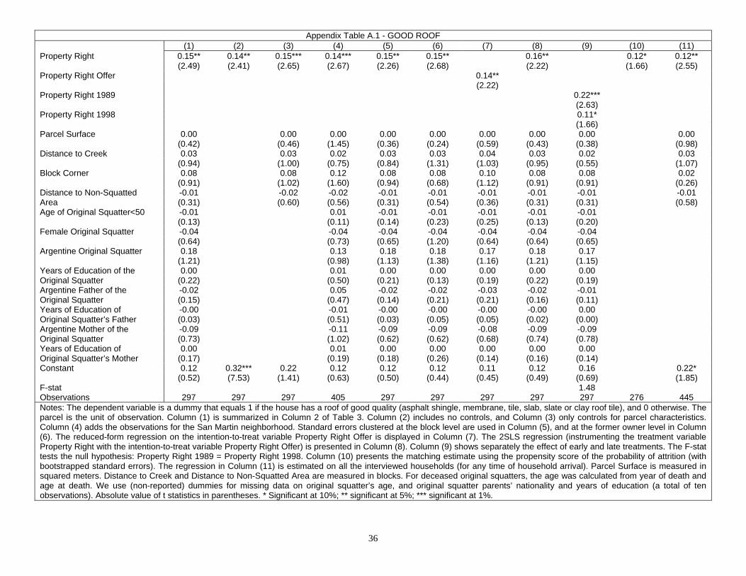
36

Appendix Table A.1 - GOOD ROOF

(1) (2) (3) (4) (5) (6) (7) (8) (9) (10) (11) Property Right 0.15** 0.14** 0.15*** 0.14*** 0.15** 0.15** 0.16** 0.12* 0.12** (2.49) (2.41) (2.65) (2.67) (2.26) (2.68) (2.22) (1.66) (2.55) Property Right Offer 0.14** (2.22) Property Right 1989 0.22*** (2.63) Property Right 1998 0.11* (1.66) Parcel Surface 0.00 0.00 0.00 0.00 0.00 0.00 0.00 0.00 0.00 (0.42) (0.46) (1.45) (0.36) (0.24) (0.59) (0.43) (0.38) (0.98) Distance to Creek 0.03 0.03 0.02 0.03 0.03 0.04 0.03 0.02 0.03 (0.94) (1.00) (0.75) (0.84) (1.31) (1.03) (0.95) (0.55) (1.07) Block Corner 0.08 0.08 0.12 0.08 0.08 0.10 0.08 0.08 0.02 (0.91) (1.02) (1.60) (0.94) (0.68) (1.12) (0.91) (0.91) (0.26) Distance to Non-Squatted -0.01 -0.02 -0.02 -0.01 -0.01 -0.01 -0.01 -0.01 -0.01 Area (0.31) (0.60) (0.56) (0.31) (0.54) (0.36) (0.31) (0.31) (0.58) Age of Original Squatter<50 -0.01 0.01 -0.01 -0.01 -0.01 -0.01 -0.01 (0.13) (0.11) (0.14) (0.23) (0.25) (0.13) (0.20) Female Original Squatter -0.04 -0.04 -0.04 -0.04 -0.04 -0.04 -0.04 (0.64) (0.73) (0.65) (1.20) (0.64) (0.64) (0.65) Argentine Original Squatter 0.18 0.13 0.18 0.18 0.17 0.18 0.17 (1.21) (0.98) (1.13) (1.38) (1.16) (1.21) (1.15) Years of Education of the 0.00 0.01 0.00 0.00 0.00 0.00 0.00 Original Squatter (0.22) (0.50) (0.21) (0.13) (0.19) (0.22) (0.19) Argentine Father of the -0.02 0.05 -0.02 -0.02 -0.03 -0.02 -0.01 Original Squatter (0.15) (0.47) (0.14) (0.21) (0.21) (0.16) (0.11) Years of Education of -0.00 -0.01 -0.00 -0.00 -0.00 -0.00 0.00 Original Squatter’s Father (0.03) (0.51) (0.03) (0.05) (0.05) (0.02) (0.00) Argentine Mother of the -0.09 -0.11 -0.09 -0.09 -0.08 -0.09 -0.09 Original Squatter (0.73) (1.02) (0.62) (0.62) (0.68) (0.74) (0.78) Years of Education of 0.00 0.01 0.00 0.00 0.00 0.00 0.00 Original Squatter’s Mother (0.17) (0.19) (0.18) (0.26) (0.14) (0.16) (0.14) Constant 0.12 0.32*** 0.22 0.12 0.12 0.12 0.11 0.12 0.16 0.22* (0.52) (7.53) (1.41) (0.63) (0.50) (0.44) (0.45) (0.49) (0.69) (1.85) F-stat 1.48 Observations 297 297 297 405 297 297 297 297 297 276 445 Notes: The dependent variable is a dummy that equals 1 if the house has a roof of good quality (asphalt shingle, membrane, tile, slab, slate or clay roof tile), and 0 otherwise. The parcel is the unit of observation. Column (1) is summarized in Column 2 of Table 3. Column (2) includes no controls, and Column (3) only controls for parcel characteristics. Column (4) adds the observations for the San Martin neighborhood. Standard errors clustered at the block level are used in Column (5), and at the former owner level in Column (6). The reduced-form regression on the intention-to-treat variable Property Right Offer is displayed in Column (7). The 2SLS regression (instrumenting the treatment variable Property Right with the intention-to-treat variable Property Right Offer) is presented in Column (8). Column (9) shows separately the effect of early and late treatments. The F-stat tests the null hypothesis: Property Right 1989 = Property Right 1998. Column (10) presents the matching estimate using the propensity score of the probability of attrition (with bootstrapped standard errors). The regression in Column (11) is estimated on all the interviewed households (for any time of household arrival). Parcel Surface is measured in squared meters. Distance to Creek and Distance to Non-Squatted Area are measured in blocks. For deceased original squatters, the age was calculated from year of death and age at death. We use (non-reported) dummies for missing data on original squatter’s age, and original squatter parents’ nationality and years of education (a total of ten observations). Absolute value of t statistics in parentheses. * Significant at 10%; ** significant at 5%; *** significant at 1%.

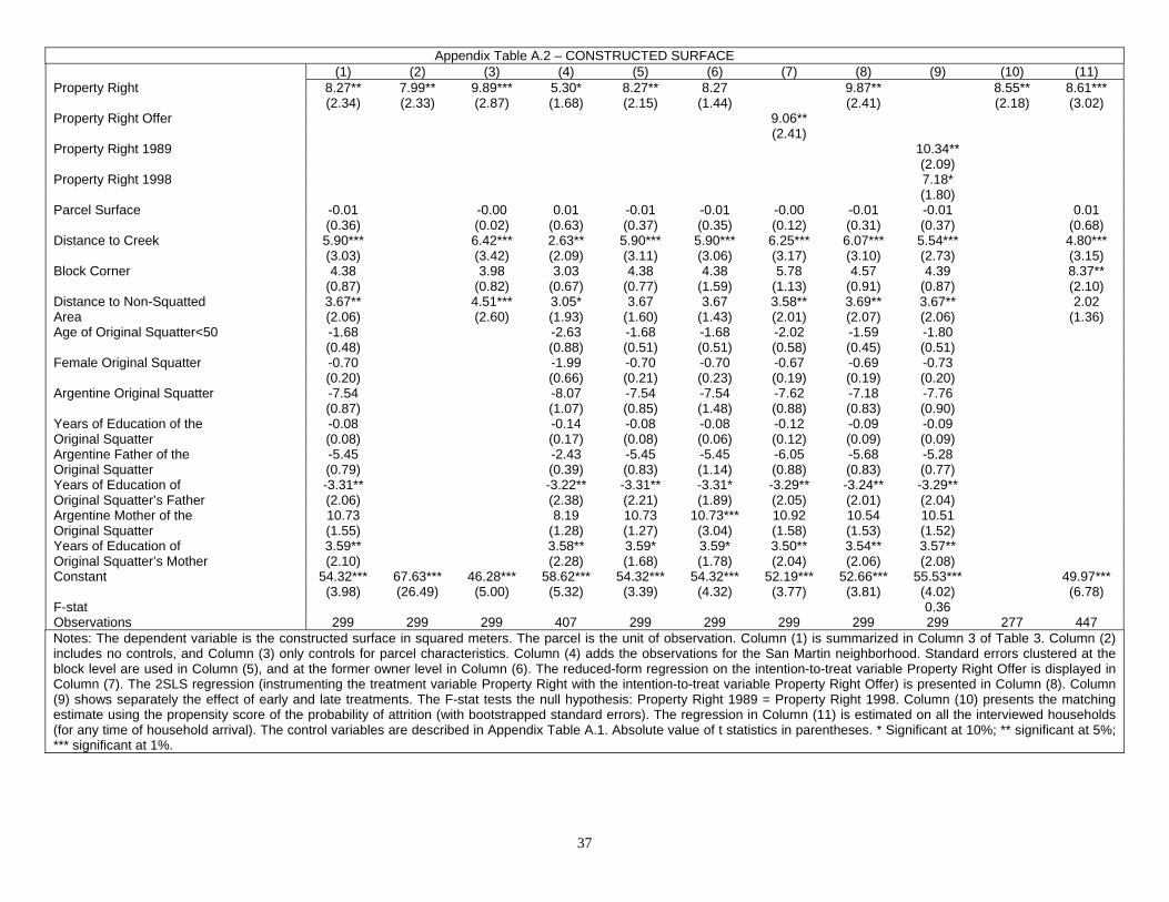
37

Appendix Table A.2 – CONSTRUCTED SURFACE

(1) (2) (3) (4) (5) (6) (7) (8) (9) (10) (11) Property Right 8.27** 7.99** 9.89*** 5.30* 8.27** 8.27 9.87** 8.55** 8.61*** (2.34) (2.33) (2.87) (1.68) (2.15) (1.44) (2.41) (2.18) (3.02) Property Right Offer 9.06** (2.41) Property Right 1989 10.34** (2.09) Property Right 1998 7.18* (1.80) Parcel Surface -0.01 -0.00 0.01 -0.01 -0.01 -0.00 -0.01 -0.01 0.01 (0.36) (0.02) (0.63) (0.37) (0.35) (0.12) (0.31) (0.37) (0.68) Distance to Creek 5.90*** 6.42*** 2.63** 5.90*** 5.90*** 6.25*** 6.07*** 5.54*** 4.80*** (3.03) (3.42) (2.09) (3.11) (3.06) (3.17) (3.10) (2.73) (3.15) Block Corner 4.38 3.98 3.03 4.38 4.38 5.78 4.57 4.39 8.37** (0.87) (0.82) (0.67) (0.77) (1.59) (1.13) (0.91) (0.87) (2.10) Distance to Non-Squatted 3.67** 4.51*** 3.05* 3.67 3.67 3.58** 3.69** 3.67** 2.02 Area (2.06) (2.60) (1.93) (1.60) (1.43) (2.01) (2.07) (2.06) (1.36) Age of Original Squatter<50 -1.68 -2.63 -1.68 -1.68 -2.02 -1.59 -1.80 (0.48) (0.88) (0.51) (0.51) (0.58) (0.45) (0.51) Female Original Squatter -0.70 -1.99 -0.70 -0.70 -0.67 -0.69 -0.73 (0.20) (0.66) (0.21) (0.23) (0.19) (0.19) (0.20) Argentine Original Squatter -7.54 -8.07 -7.54 -7.54 -7.62 -7.18 -7.76 (0.87) (1.07) (0.85) (1.48) (0.88) (0.83) (0.90) Years of Education of the -0.08 -0.14 -0.08 -0.08 -0.12 -0.09 -0.09 Original Squatter (0.08) (0.17) (0.08) (0.06) (0.12) (0.09) (0.09) Argentine Father of the -5.45 -2.43 -5.45 -5.45 -6.05 -5.68 -5.28 Original Squatter (0.79) (0.39) (0.83) (1.14) (0.88) (0.83) (0.77) Years of Education of -3.31** -3.22** -3.31** -3.31* -3.29** -3.24** -3.29** Original Squatter’s Father (2.06) (2.38) (2.21) (1.89) (2.05) (2.01) (2.04) Argentine Mother of the 10.73 8.19 10.73 10.73*** 10.92 10.54 10.51 Original Squatter (1.55) (1.28) (1.27) (3.04) (1.58) (1.53) (1.52) Years of Education of 3.59** 3.58** 3.59* 3.59* 3.50** 3.54** 3.57** Original Squatter’s Mother (2.10) (2.28) (1.68) (1.78) (2.04) (2.06) (2.08) Constant 54.32*** 67.63*** 46.28*** 58.62*** 54.32*** 54.32*** 52.19*** 52.66*** 55.53*** 49.97*** (3.98) (26.49) (5.00) (5.32) (3.39) (4.32) (3.77) (3.81) (4.02) (6.78) F-stat 0.36 Observations 299 299 299 407 299 299 299 299 299 277 447 Notes: The dependent variable is the constructed surface in squared meters. The parcel is the unit of observation. Column (1) is summarized in Column 3 of Table 3. Column (2) includes no controls, and Column (3) only controls for parcel characteristics. Column (4) adds the observations for the San Martin neighborhood. Standard errors clustered at the block level are used in Column (5), and at the former owner level in Column (6). The reduced-form regression on the intention-to-treat variable Property Right Offer is displayed in Column (7). The 2SLS regression (instrumenting the treatment variable Property Right with the intention-to-treat variable Property Right Offer) is presented in Column (8). Column (9) shows separately the effect of early and late treatments. The F-stat tests the null hypothesis: Property Right 1989 = Property Right 1998. Column (10) presents the matching estimate using the propensity score of the probability of attrition (with bootstrapped standard errors). The regression in Column (11) is estimated on all the interviewed households (for any time of household arrival). The control variables are described in Appendix Table A.1. Absolute value of t statistics in parentheses. * Significant at 10%; ** significant at 5%; *** significant at 1%.

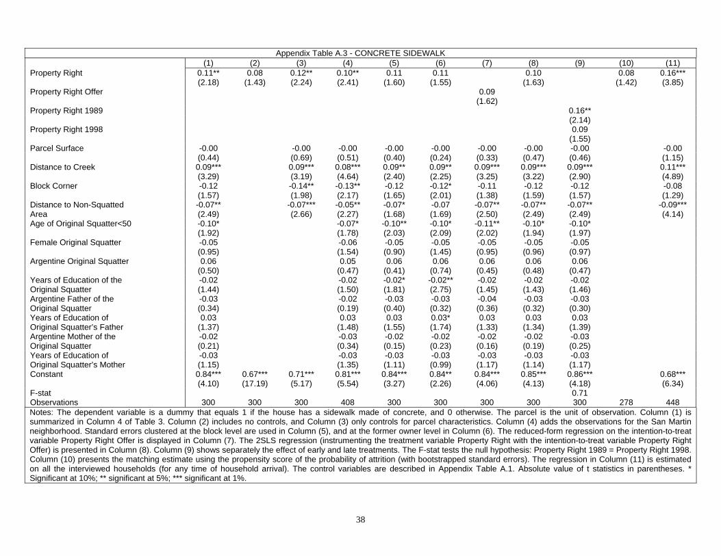
38

Appendix Table A.3 - CONCRETE SIDEWALK (1) (2) (3) (4) (5) (6) (7) (8) (9) (10) (11) Property Right 0.11** 0.08 0.12** 0.10** 0.11 0.11 0.10 0.08 0.16*** (2.18) (1.43) (2.24) (2.41) (1.60) (1.55) (1.63) (1.42) (3.85) Property Right Offer 0.09 (1.62) Property Right 1989 0.16** (2.14) Property Right 1998 0.09 (1.55) Parcel Surface -0.00 -0.00 -0.00 -0.00 -0.00 -0.00 -0.00 -0.00 -0.00 (0.44) (0.69) (0.51) (0.40) (0.24) (0.33) (0.47) (0.46) (1.15) Distance to Creek 0.09*** 0.09*** 0.08*** 0.09** 0.09** 0.09*** 0.09*** 0.09*** 0.11*** (3.29) (3.19) (4.64) (2.40) (2.25) (3.25) (3.22) (2.90) (4.89) Block Corner -0.12 -0.14** -0.13** -0.12 -0.12* -0.11 -0.12 -0.12 -0.08 (1.57) (1.98) (2.17) (1.65) (2.01) (1.38) (1.59) (1.57) (1.29) Distance to Non-Squatted -0.07** -0.07*** -0.05** -0.07* -0.07 -0.07** -0.07** -0.07** -0.09*** Area (2.49) (2.66) (2.27) (1.68) (1.69) (2.50) (2.49) (2.49) (4.14) Age of Original Squatter<50 -0.10* -0.07* -0.10** -0.10* -0.11** -0.10* -0.10* (1.92) (1.78) (2.03) (2.09) (2.02) (1.94) (1.97) Female Original Squatter -0.05 -0.06 -0.05 -0.05 -0.05 -0.05 -0.05 (0.95) (1.54) (0.90) (1.45) (0.95) (0.96) (0.97) Argentine Original Squatter 0.06 0.05 0.06 0.06 0.06 0.06 0.06 (0.50) (0.47) (0.41) (0.74) (0.45) (0.48) (0.47) Years of Education of the -0.02 -0.02 -0.02* -0.02** -0.02 -0.02 -0.02 Original Squatter (1.44) (1.50) (1.81) (2.75) (1.45) (1.43) (1.46) Argentine Father of the -0.03 -0.02 -0.03 -0.03 -0.04 -0.03 -0.03 Original Squatter (0.34) (0.19) (0.40) (0.32) (0.36) (0.32) (0.30) Years of Education of 0.03 0.03 0.03 0.03* 0.03 0.03 0.03 Original Squatter’s Father (1.37) (1.48) (1.55) (1.74) (1.33) (1.34) (1.39) Argentine Mother of the -0.02 -0.03 -0.02 -0.02 -0.02 -0.02 -0.03 Original Squatter (0.21) (0.34) (0.15) (0.23) (0.16) (0.19) (0.25) Years of Education of -0.03 -0.03 -0.03 -0.03 -0.03 -0.03 -0.03 Original Squatter’s Mother (1.15) (1.35) (1.11) (0.99) (1.17) (1.14) (1.17) Constant 0.84*** 0.67*** 0.71*** 0.81*** 0.84*** 0.84** 0.84*** 0.85*** 0.86*** 0.68*** (4.10) (17.19) (5.17) (5.54) (3.27) (2.26) (4.06) (4.13) (4.18) (6.34) F-stat 0.71 Observations 300 300 300 408 300 300 300 300 300 278 448 Notes: The dependent variable is a dummy that equals 1 if the house has a sidewalk made of concrete, and 0 otherwise. The parcel is the unit of observation. Column (1) is summarized in Column 4 of Table 3. Column (2) includes no controls, and Column (3) only controls for parcel characteristics. Column (4) adds the observations for the San Martin neighborhood. Standard errors clustered at the block level are used in Column (5), and at the former owner level in Column (6). The reduced-form regression on the intention-to-treat variable Property Right Offer is displayed in Column (7). The 2SLS regression (instrumenting the treatment variable Property Right with the intention-to-treat variable Property Right Offer) is presented in Column (8). Column (9) shows separately the effect of early and late treatments. The F-stat tests the null hypothesis: Property Right 1989 = Property Right 1998. Column (10) presents the matching estimate using the propensity score of the probability of attrition (with bootstrapped standard errors). The regression in Column (11) is estimated on all the interviewed households (for any time of household arrival). The control variables are described in Appendix Table A.1. Absolute value of t statistics in parentheses. * Significant at 10%; ** significant at 5%; *** significant at 1%.

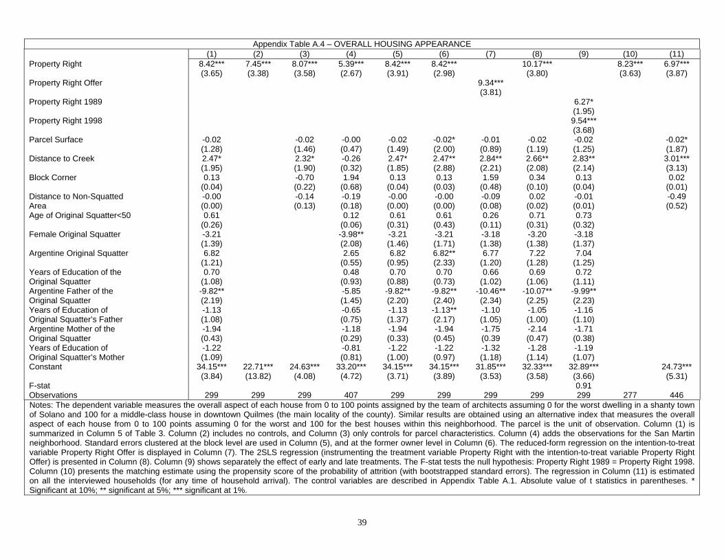
39

Appendix Table A.4 – OVERALL HOUSING APPEARANCE (1) (2) (3) (4) (5) (6) (7) (8) (9) (10) (11) Property Right 8.42*** 7.45*** 8.07*** 5.39*** 8.42*** 8.42*** 10.17*** 8.23*** 6.97*** (3.65) (3.38) (3.58) (2.67) (3.91) (2.98) (3.80) (3.63) (3.87) Property Right Offer 9.34*** (3.81) Property Right 1989 6.27* (1.95) Property Right 1998 9.54*** (3.68) Parcel Surface -0.02 -0.02 -0.00 -0.02 -0.02* -0.01 -0.02 -0.02 -0.02* (1.28) (1.46) (0.47) (1.49) (2.00) (0.89) (1.19) (1.25) (1.87) Distance to Creek 2.47* 2.32* -0.26 2.47* 2.47** 2.84** 2.66** 2.83** 3.01*** (1.95) (1.90) (0.32) (1.85) (2.88) (2.21) (2.08) (2.14) (3.13) Block Corner 0.13 -0.70 1.94 0.13 0.13 1.59 0.34 0.13 0.02 (0.04) (0.22) (0.68) (0.04) (0.03) (0.48) (0.10) (0.04) (0.01) Distance to Non-Squatted -0.00 -0.14 -0.19 -0.00 -0.00 -0.09 0.02 -0.01 -0.49 Area (0.00) (0.13) (0.18) (0.00) (0.00) (0.08) (0.02) (0.01) (0.52) Age of Original Squatter<50 0.61 0.12 0.61 0.61 0.26 0.71 0.73 (0.26) (0.06) (0.31) (0.43) (0.11) (0.31) (0.32) Female Original Squatter -3.21 -3.98** -3.21 -3.21 -3.18 -3.20 -3.18 (1.39) (2.08) (1.46) (1.71) (1.38) (1.38) (1.37) Argentine Original Squatter 6.82 2.65 6.82 6.82** 6.77 7.22 7.04 (1.21) (0.55) (0.95) (2.33) (1.20) (1.28) (1.25) Years of Education of the 0.70 0.48 0.70 0.70 0.66 0.69 0.72 Original Squatter (1.08) (0.93) (0.88) (0.73) (1.02) (1.06) (1.11) Argentine Father of the -9.82** -5.85 -9.82** -9.82** -10.46** -10.07** -9.99** Original Squatter (2.19) (1.45) (2.20) (2.40) (2.34) (2.25) (2.23) Years of Education of -1.13 -0.65 -1.13 -1.13** -1.10 -1.05 -1.16 Original Squatter’s Father (1.08) (0.75) (1.37) (2.17) (1.05) (1.00) (1.10) Argentine Mother of the -1.94 -1.18 -1.94 -1.94 -1.75 -2.14 -1.71 Original Squatter (0.43) (0.29) (0.33) (0.45) (0.39 (0.47) (0.38) Years of Education of -1.22 -0.81 -1.22 -1.22 -1.32 -1.28 -1.19 Original Squatter’s Mother (1.09) (0.81) (1.00) (0.97) (1.18) (1.14) (1.07) Constant 34.15*** 22.71*** 24.63*** 33.20*** 34.15*** 34.15*** 31.85*** 32.33*** 32.89*** 24.73*** (3.84) (13.82) (4.08) (4.72) (3.71) (3.89) (3.53) (3.58) (3.66) (5.31) F-stat 0.91 Observations 299 299 299 407 299 299 299 299 299 277 446 Notes: The dependent variable measures the overall aspect of each house from 0 to 100 points assigned by the team of architects assuming 0 for the worst dwelling in a shanty town of Solano and 100 for a middle-class house in downtown Quilmes (the main locality of the county). Similar results are obtained using an alternative index that measures the overall aspect of each house from 0 to 100 points assuming 0 for the worst and 100 for the best houses within this neighborhood. The parcel is the unit of observation. Column (1) is summarized in Column 5 of Table 3. Column (2) includes no controls, and Column (3) only controls for parcel characteristics. Column (4) adds the observations for the San Martin neighborhood. Standard errors clustered at the block level are used in Column (5), and at the former owner level in Column (6). The reduced-form regression on the intention-to-treat variable Property Right Offer is displayed in Column (7). The 2SLS regression (instrumenting the treatment variable Property Right with the intention-to-treat variable Property Right Offer) is presented in Column (8). Column (9) shows separately the effect of early and late treatments. The F-stat tests the null hypothesis: Property Right 1989 = Property Right 1998. Column (10) presents the matching estimate using the propensity score of the probability of attrition (with bootstrapped standard errors). The regression in Column (11) is estimated on all the interviewed households (for any time of household arrival). The control variables are described in Appendix Table A.1. Absolute value of t statistics in parentheses. * Significant at 10%; ** significant at 5%; *** significant at 1%.

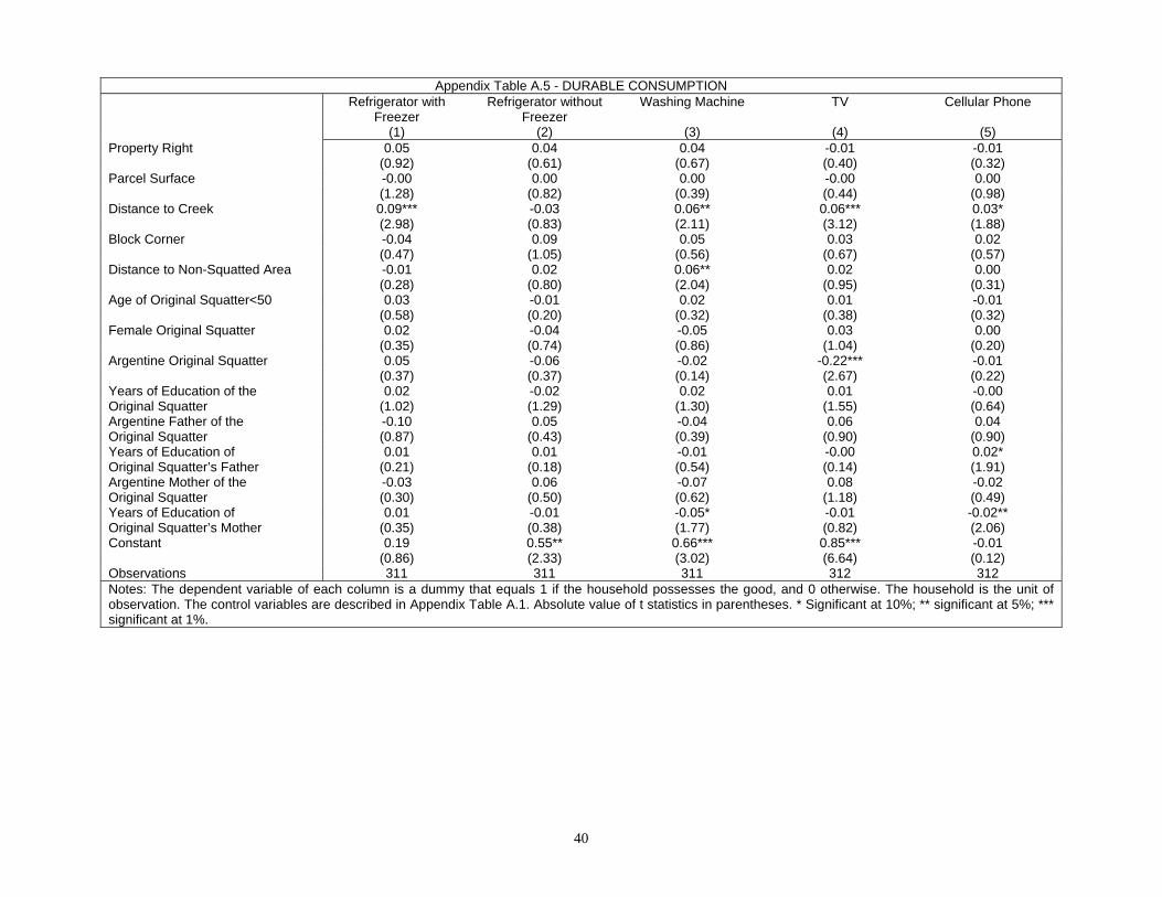
40

Appendix Table A.5 - DURABLE CONSUMPTION Refrigerator with

Freezer (1)

Refrigerator without Freezer

(2)

Washing Machine

(3)

TV

(4)

Cellular Phone

(5) Property Right 0.05 0.04 0.04 -0.01 -0.01 (0.92) (0.61) (0.67) (0.40) (0.32) Parcel Surface -0.00 0.00 0.00 -0.00 0.00 (1.28) (0.82) (0.39) (0.44) (0.98) Distance to Creek 0.09*** -0.03 0.06** 0.06*** 0.03* (2.98) (0.83) (2.11) (3.12) (1.88) Block Corner -0.04 0.09 0.05 0.03 0.02 (0.47) (1.05) (0.56) (0.67) (0.57) Distance to Non-Squatted Area -0.01 0.02 0.06** 0.02 0.00 (0.28) (0.80) (2.04) (0.95) (0.31) Age of Original Squatter<50 0.03 -0.01 0.02 0.01 -0.01 (0.58) (0.20) (0.32) (0.38) (0.32) Female Original Squatter 0.02 -0.04 -0.05 0.03 0.00 (0.35) (0.74) (0.86) (1.04) (0.20) Argentine Original Squatter 0.05 -0.06 -0.02 -0.22*** -0.01 (0.37) (0.37) (0.14) (2.67) (0.22) Years of Education of the 0.02 -0.02 0.02 0.01 -0.00 Original Squatter (1.02) (1.29) (1.30) (1.55) (0.64) Argentine Father of the -0.10 0.05 -0.04 0.06 0.04 Original Squatter (0.87) (0.43) (0.39) (0.90) (0.90) Years of Education of 0.01 0.01 -0.01 -0.00 0.02* Original Squatter’s Father (0.21) (0.18) (0.54) (0.14) (1.91) Argentine Mother of the -0.03 0.06 -0.07 0.08 -0.02 Original Squatter (0.30) (0.50) (0.62) (1.18) (0.49) Years of Education of 0.01 -0.01 -0.05* -0.01 -0.02** Original Squatter’s Mother (0.35) (0.38) (1.77) (0.82) (2.06) Constant 0.19 0.55** 0.66*** 0.85*** -0.01 (0.86) (2.33) (3.02) (6.64) (0.12) Observations 311 311 311 312 312 Notes: The dependent variable of each column is a dummy that equals 1 if the household possesses the good, and 0 otherwise. The household is the unit of observation. The control variables are described in Appendix Table A.1. Absolute value of t statistics in parentheses. * Significant at 10%; ** significant at 5%; *** significant at 1%.

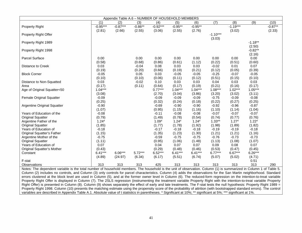
41

Appendix Table A.6 – NUMBER OF HOUSEHOLD MEMBERS (1) (2) (3) (4) (5) (6) (7) (8) (9) (10) Property Right -0.95*** -0.87*** -0.86** -0.92*** -0.95** -0.95** -1.19*** -0.87** (2.81) (2.66) (2.55) (3.06) (2.55) (2.76) (3.02) (2.33) Property Right Offer -1.10*** (3.03) Property Right 1989 -1.18** (2.50) Property Right 1998 -0.82** (2.16) Parcel Surface 0.00 0.00 0.00 0.00 0.00 0.00 0.00 0.00 (0.58) (0.68) (0.86) (0.61) (1.12) (0.22) (0.51) (0.60) Distance to Creek 0.03 -0.04 0.08 0.03 0.03 -0.02 0.01 0.07 (0.19) (0.20) (0.66) (0.19) (0.21) (0.12) (0.05) (0.39) Block Corner -0.05 0.05 0.03 -0.05 -0.05 -0.25 -0.07 -0.05 (0.10) (0.10) (0.06) (0.11) (0.12) (0.51) (0.15) (0.10) Distance to Non-Squatted 0.03 -0.02 0.10 0.03 0.03 0.04 0.03 0.03 Area (0.17) (0.11) (0.64) (0.17) (0.19) (0.21) (0.16) (0.17) Age of Original Squatter<50 1.04*** 0.77*** 1.04*** 1.04*** 1.08*** 1.02*** 1.05*** (3.08) (2.70) (3.04) (3.86) (3.20) (3.02) (3.11) Female Original Squatter -0.09 -0.09 -0.09 -0.09 -0.75 -0.09 -0.08 (0.25) (0.32) (0.24) (0.18) (0.22) (0.27) (0.25) Argentine Original Squatter -0.90 -0.69 -0.90 -0.90 -0.92 -0.96 -0.87 (1.07) (0.95) (1.15) (1.16) (1.10) (1.14) (1.04) Years of Education of the -0.08 -0.11 -0.08 -0.08 -0.07 -0.07 -0.07 Original Squatter (0.79) (1.49) (0.78) (0.54) (0.74) (0.77) (0.76) Argentine Father of the 1.24* 1.09* 1.24* 1.24* 1.33** 1.27* 1.22* Original Squatter (1.85) (1.77) (1.78) (1.92) (1.98) (1.89) (1.82) Years of Education of -0.18 -0.17 -0.18 -0.18 -0.19 -0.19 -0.18 Original Squatter’s Father (1.15) (1.35) (1.23) (1.30) (1.21) (1.21) (1.16) Argentine Mother of the -0.75 -0.59 -0.75 -0.75 -0.76 -0.73 -0.73 Original Squatter (1.11) (0.95) (1.06) (1.48) (1.13) (1.08) (1.07) Years of Education of 0.07 0.04 0.07 0.07 0.09 0.08 0.07 Original Squatter’s Mother (0.43) (0.29) (0.48) (0.46) (0.53) (0.47) (0.45) Constant 6.41*** 6.06*** 5.72*** 6.52*** 6.41*** 6.41*** 6.77*** 6.67*** 6.26*** (4.89) (24.97) (6.34) (6.17) (5.51) (6.74) (5.07) (5.02) (4.71) F-stat 0.51 Observations 313 313 313 425 313 313 313 313 313 290 Notes: The dependent variable is the total number of household members. The household is the unit of observation. Column (1) is summarized in Column 1 of Table 5. Column (2) includes no controls, and Column (3) only controls for parcel characteristics. Column (4) adds the observations for the San Martin neighborhood. Standard errors clustered at the block level are used in Column (5), and at the former owner level in Column (6). The reduced-form regression on the intention-to-treat variable Property Right Offer is displayed in Column (7). The 2SLS regression (instrumenting the treatment variable Property Right with the intention-to-treat variable Property Right Offer) is presented in Column (8). Column (9) shows separately the effect of early and late treatments. The F-stat tests the null hypothesis: Property Right 1989 = Property Right 1998. Column (10) presents the matching estimate using the propensity score of the probability of attrition (with bootstrapped standard errors). The control variables are described in Appendix Table A.1. Absolute value of t statistics in parentheses. * Significant at 10%; ** significant at 5%; *** significant at 1%.

42

Appendix Table A.7 – HOUSEHOLD HEAD SPOUSE (1) (2) (3) (4) (5) (6) (7) (8) (9) (10) Property Right -0.01 -0.02 -0.02 -0.03 -0.01 -0.01 0.01 -0.05 (0.27) (0.37) (0.37) (0.56) (0.26) (0.41) (0.20) (0.70) Property Right Offer 0.01 (0.20) Property Right 1989 -0.03 (0.36) Property Right 1998 -0.01 (0.13) Parcel Surface -0.00 -0.00 -0.00 -0.00 -0.00 -0.00 -0.00 -0.00 (0.94) (1.45) (0.86) (0.98) (1.53) (0.86) (0.89) (0.93) Distance to Creek 0.02 0.01 0.01 0.02 0.02 0.02 0.02 0.02 (0.67) (0.47) (0.73) (0.70) (0.58) (0.75) (0.75) (0.70) Block Corner 0.03 0.06 0.03 0.03 0.03 0.03 0.03 0.03 (0.41) (0.84) (0.44) (0.44) (0.45) (0.46) (0.45) (0.41) Distance to Non-Squatted 0.01 0.00 0.03 0.01 0.01 0.01 0.01 0.01 Area (0.37) (0.03) (1.22) (0.36) (0.39) (0.37) (0.37) (0.37) Age of Original Squatter<50 0.03 0.04 0.03 0.03 0.03 0.03 0.03 (0.56) (1.02) (0.47) (0.57) (0.58) (0.59) (0.57) Female Original Squatter -0.28*** -0.31*** -0.28*** -0.28*** -0.28*** -0.28*** -0.28*** (5.41) (7.20) (4.82) (4.66) (5.40) (5.39) (5.40) Argentine Original Squatter -0.01 0.01 -0.01 -0.01 -0.00 0.00 -0.00 (0.05) (0.14) (0.05) (0.04) (0.00) (0.00) (0.04) Years of Education of the 0.02* 0.01 0.02* 0.02** 0.02* 0.02* 0.02* Original Squatter (1.71) (1.02) (1.77) (2.22) (1.70) (1.71) (1.72) Argentine Father of the -0.05 -0.02 -0.05 -0.05 -0.05 -0.05 -0.05 Original Squatter (0.45) (0.24) (0.55) (0.77) (0.48) (0.48) (0.45) Years of Education of 0.00 0.02 0.00 0.00 0.00 0.00 0.00 Original Squatter’s Father (0.03) (0.85) (0.03) (0.03) (0.07) (0.07) (0.02) Argentine Mother of the -0.06 -0.09 -0.06 -0.06 -0.06 -0.06 -0.06 Original Squatter (0.58) (0.93) (0.63) (0.53) (0.60) (0.60) (0.56) Years of Education of -0.02 0.00 -0.02 -0.02 -0.02 -0.02 -0.02 Original Squatter’s Mother (0.81) (0.12) (0.64) (0.85) (0.84) (0.83) (0.80) Constant 0.89*** 0.74*** 0.84*** 0.73*** 0.89*** 0.89*** 0.86*** 0.86*** 0.88*** (4.46) (19.44) (6.01) (4.59) (5.25) (9.38) (4.23) (4.27) (4.36) F-stat 0.06 Observations 313 313 313 425 313 313 313 313 313 290 Notes: The dependent variable is a dummy that equals 1 if the household head lives with a spouse, and 0 otherwise. The household is the unit of observation. Column (1) is summarized in Column 2 of Table 5. Column (2) includes no controls, and Column (3) only controls for parcel characteristics. Column (4) adds the observations for the San Martin neighborhood. Standard errors clustered at the block level are used in Column (5), and at the former owner level in Column (6). The reduced-form regression on the intention-to-treat variable Property Right Offer is displayed in Column (7). The 2SLS regression (instrumenting the treatment variable Property Right with the intention-to-treat variable Property Right Offer) is presented in Column (8). Column (9) shows separately the effect of early and late treatments. The F-stat tests the null hypothesis: Property Right 1989 = Property Right 1998. Column (10) presents the matching estimate using the propensity score of the probability of attrition (with bootstrapped standard errors). The control variables are described in Appendix Table A.1. Absolute value of t statistics in parentheses. * Significant at 10%; ** significant at 5%; *** significant at 1%.

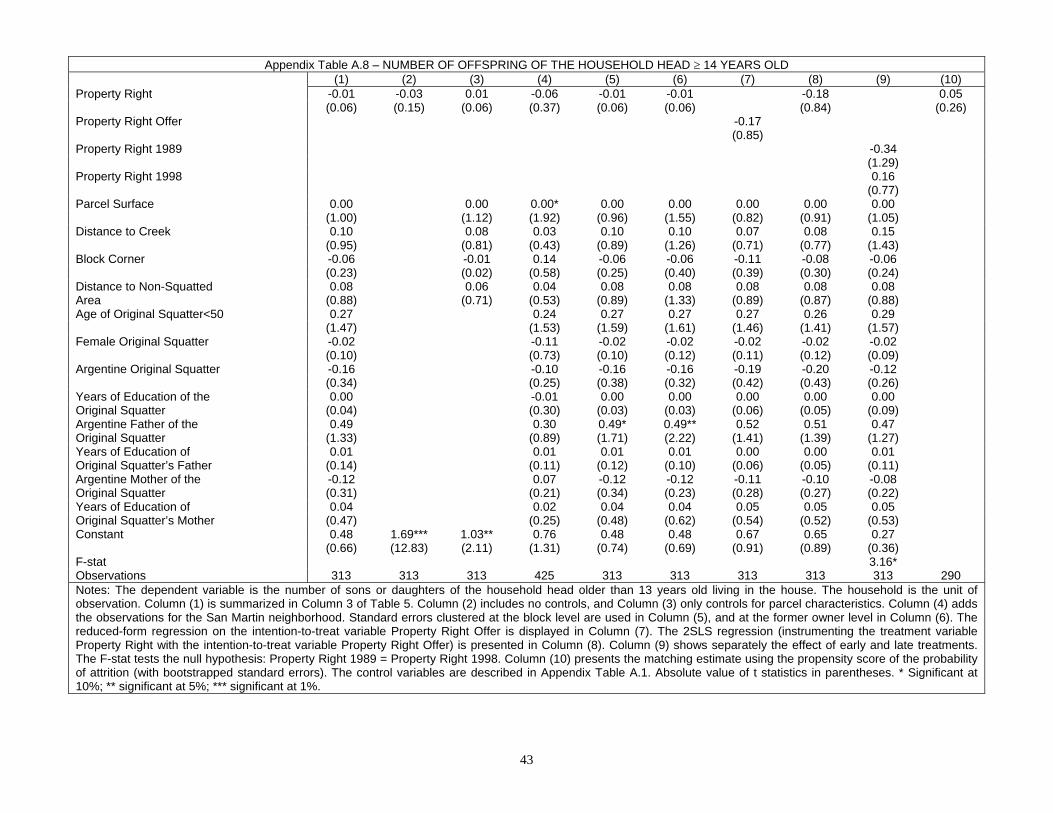
43

Appendix Table A.8 – NUMBER OF OFFSPRING OF THE HOUSEHOLD HEAD ≥ 14 YEARS OLD (1) (2) (3) (4) (5) (6) (7) (8) (9) (10) Property Right -0.01 -0.03 0.01 -0.06 -0.01 -0.01 -0.18 0.05 (0.06) (0.15) (0.06) (0.37) (0.06) (0.06) (0.84) (0.26) Property Right Offer -0.17 (0.85) Property Right 1989 -0.34 (1.29) Property Right 1998 0.16 (0.77) Parcel Surface 0.00 0.00 0.00* 0.00 0.00 0.00 0.00 0.00 (1.00) (1.12) (1.92) (0.96) (1.55) (0.82) (0.91) (1.05) Distance to Creek 0.10 0.08 0.03 0.10 0.10 0.07 0.08 0.15 (0.95) (0.81) (0.43) (0.89) (1.26) (0.71) (0.77) (1.43) Block Corner -0.06 -0.01 0.14 -0.06 -0.06 -0.11 -0.08 -0.06 (0.23) (0.02) (0.58) (0.25) (0.40) (0.39) (0.30) (0.24) Distance to Non-Squatted 0.08 0.06 0.04 0.08 0.08 0.08 0.08 0.08 Area (0.88) (0.71) (0.53) (0.89) (1.33) (0.89) (0.87) (0.88) Age of Original Squatter<50 0.27 0.24 0.27 0.27 0.27 0.26 0.29 (1.47) (1.53) (1.59) (1.61) (1.46) (1.41) (1.57) Female Original Squatter -0.02 -0.11 -0.02 -0.02 -0.02 -0.02 -0.02 (0.10) (0.73) (0.10) (0.12) (0.11) (0.12) (0.09) Argentine Original Squatter -0.16 -0.10 -0.16 -0.16 -0.19 -0.20 -0.12 (0.34) (0.25) (0.38) (0.32) (0.42) (0.43) (0.26) Years of Education of the 0.00 -0.01 0.00 0.00 0.00 0.00 0.00 Original Squatter (0.04) (0.30) (0.03) (0.03) (0.06) (0.05) (0.09) Argentine Father of the 0.49 0.30 0.49* 0.49** 0.52 0.51 0.47 Original Squatter (1.33) (0.89) (1.71) (2.22) (1.41) (1.39) (1.27) Years of Education of 0.01 0.01 0.01 0.01 0.00 0.00 0.01 Original Squatter’s Father (0.14) (0.11) (0.12) (0.10) (0.06) (0.05) (0.11) Argentine Mother of the -0.12 0.07 -0.12 -0.12 -0.11 -0.10 -0.08 Original Squatter (0.31) (0.21) (0.34) (0.23) (0.28) (0.27) (0.22) Years of Education of 0.04 0.02 0.04 0.04 0.05 0.05 0.05 Original Squatter’s Mother (0.47) (0.25) (0.48) (0.62) (0.54) (0.52) (0.53) Constant 0.48 1.69*** 1.03** 0.76 0.48 0.48 0.67 0.65 0.27 (0.66) (12.83) (2.11) (1.31) (0.74) (0.69) (0.91) (0.89) (0.36) F-stat 3.16* Observations 313 313 313 425 313 313 313 313 313 290 Notes: The dependent variable is the number of sons or daughters of the household head older than 13 years old living in the house. The household is the unit of observation. Column (1) is summarized in Column 3 of Table 5. Column (2) includes no controls, and Column (3) only controls for parcel characteristics. Column (4) adds the observations for the San Martin neighborhood. Standard errors clustered at the block level are used in Column (5), and at the former owner level in Column (6). The reduced-form regression on the intention-to-treat variable Property Right Offer is displayed in Column (7). The 2SLS regression (instrumenting the treatment variable Property Right with the intention-to-treat variable Property Right Offer) is presented in Column (8). Column (9) shows separately the effect of early and late treatments. The F-stat tests the null hypothesis: Property Right 1989 = Property Right 1998. Column (10) presents the matching estimate using the propensity score of the probability of attrition (with bootstrapped standard errors). The control variables are described in Appendix Table A.1. Absolute value of t statistics in parentheses. * Significant at 10%; ** significant at 5%; *** significant at 1%.

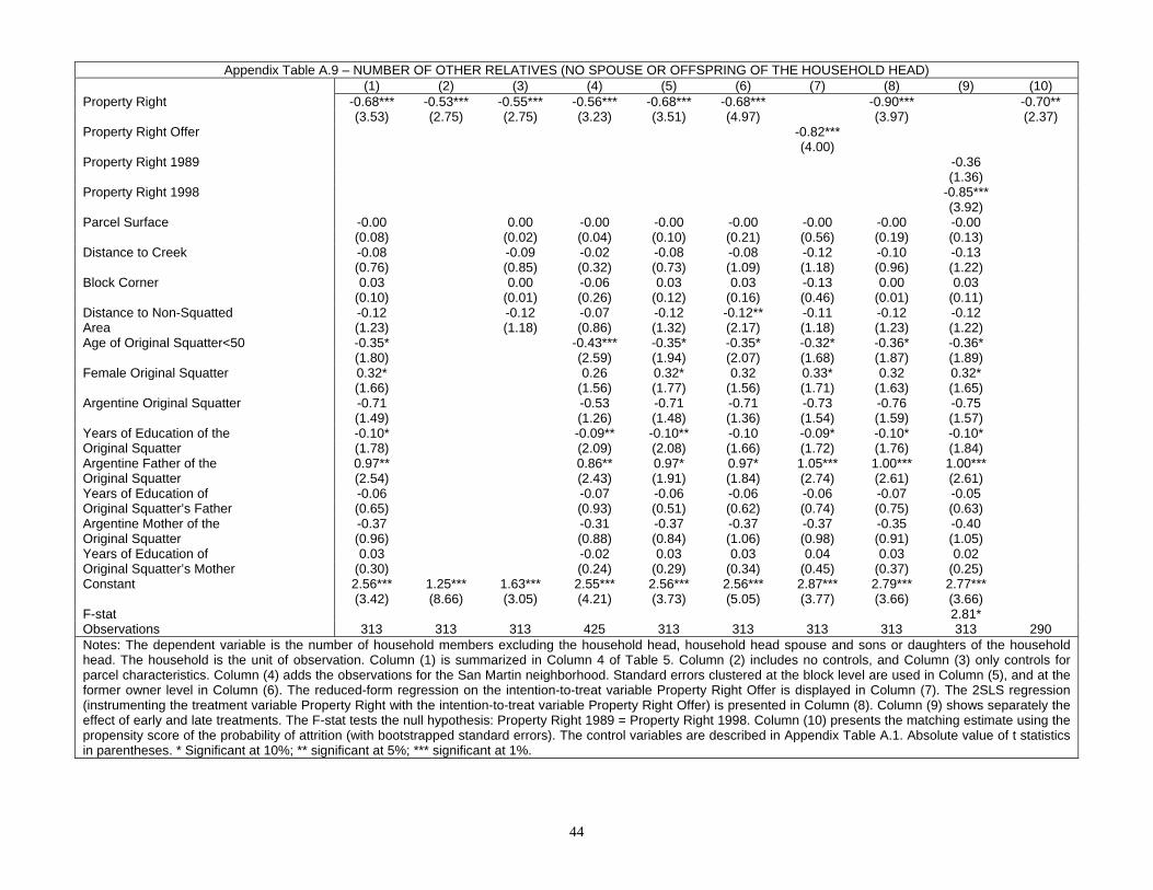
44

Appendix Table A.9 – NUMBER OF OTHER RELATIVES (NO SPOUSE OR OFFSPRING OF THE HOUSEHOLD HEAD) (1) (2) (3) (4) (5) (6) (7) (8) (9) (10) Property Right -0.68*** -0.53*** -0.55*** -0.56*** -0.68*** -0.68*** -0.90*** -0.70** (3.53) (2.75) (2.75) (3.23) (3.51) (4.97) (3.97) (2.37) Property Right Offer -0.82*** (4.00) Property Right 1989 -0.36 (1.36) Property Right 1998 -0.85*** (3.92) Parcel Surface -0.00 0.00 -0.00 -0.00 -0.00 -0.00 -0.00 -0.00 (0.08) (0.02) (0.04) (0.10) (0.21) (0.56) (0.19) (0.13) Distance to Creek -0.08 -0.09 -0.02 -0.08 -0.08 -0.12 -0.10 -0.13 (0.76) (0.85) (0.32) (0.73) (1.09) (1.18) (0.96) (1.22) Block Corner 0.03 0.00 -0.06 0.03 0.03 -0.13 0.00 0.03 (0.10) (0.01) (0.26) (0.12) (0.16) (0.46) (0.01) (0.11) Distance to Non-Squatted -0.12 -0.12 -0.07 -0.12 -0.12** -0.11 -0.12 -0.12 Area (1.23) (1.18) (0.86) (1.32) (2.17) (1.18) (1.23) (1.22) Age of Original Squatter<50 -0.35* -0.43*** -0.35* -0.35* -0.32* -0.36* -0.36* (1.80) (2.59) (1.94) (2.07) (1.68) (1.87) (1.89) Female Original Squatter 0.32* 0.26 0.32* 0.32 0.33* 0.32 0.32* (1.66) (1.56) (1.77) (1.56) (1.71) (1.63) (1.65) Argentine Original Squatter -0.71 -0.53 -0.71 -0.71 -0.73 -0.76 -0.75 (1.49) (1.26) (1.48) (1.36) (1.54) (1.59) (1.57) Years of Education of the -0.10* -0.09** -0.10** -0.10 -0.09* -0.10* -0.10* Original Squatter (1.78) (2.09) (2.08) (1.66) (1.72) (1.76) (1.84) Argentine Father of the 0.97** 0.86** 0.97* 0.97* 1.05*** 1.00*** 1.00*** Original Squatter (2.54) (2.43) (1.91) (1.84) (2.74) (2.61) (2.61) Years of Education of -0.06 -0.07 -0.06 -0.06 -0.06 -0.07 -0.05 Original Squatter’s Father (0.65) (0.93) (0.51) (0.62) (0.74) (0.75) (0.63) Argentine Mother of the -0.37 -0.31 -0.37 -0.37 -0.37 -0.35 -0.40 Original Squatter (0.96) (0.88) (0.84) (1.06) (0.98) (0.91) (1.05) Years of Education of 0.03 -0.02 0.03 0.03 0.04 0.03 0.02 Original Squatter’s Mother (0.30) (0.24) (0.29) (0.34) (0.45) (0.37) (0.25) Constant 2.56*** 1.25*** 1.63*** 2.55*** 2.56*** 2.56*** 2.87*** 2.79*** 2.77*** (3.42) (8.66) (3.05) (4.21) (3.73) (5.05) (3.77) (3.66) (3.66) F-stat 2.81* Observations 313 313 313 425 313 313 313 313 313 290 Notes: The dependent variable is the number of household members excluding the household head, household head spouse and sons or daughters of the household head. The household is the unit of observation. Column (1) is summarized in Column 4 of Table 5. Column (2) includes no controls, and Column (3) only controls for parcel characteristics. Column (4) adds the observations for the San Martin neighborhood. Standard errors clustered at the block level are used in Column (5), and at the former owner level in Column (6). The reduced-form regression on the intention-to-treat variable Property Right Offer is displayed in Column (7). The 2SLS regression (instrumenting the treatment variable Property Right with the intention-to-treat variable Property Right Offer) is presented in Column (8). Column (9) shows separately the effect of early and late treatments. The F-stat tests the null hypothesis: Property Right 1989 = Property Right 1998. Column (10) presents the matching estimate using the propensity score of the probability of attrition (with bootstrapped standard errors). The control variables are described in Appendix Table A.1. Absolute value of t statistics in parentheses. * Significant at 10%; ** significant at 5%; *** significant at 1%.

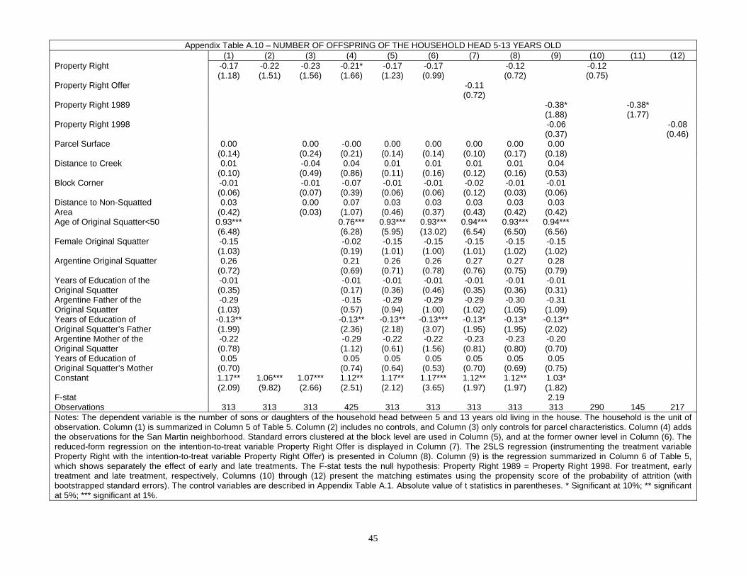
45

Appendix Table A.10 – NUMBER OF OFFSPRING OF THE HOUSEHOLD HEAD 5-13 YEARS OLD (1) (2) (3) (4) (5) (6) (7) (8) (9) (10) (11) (12) Property Right -0.17 -0.22 -0.23 -0.21* -0.17 -0.17 -0.12 -0.12 (1.18) (1.51) (1.56) (1.66) (1.23) (0.99) (0.72) (0.75) Property Right Offer -0.11 (0.72) Property Right 1989 -0.38* -0.38* (1.88) (1.77) Property Right 1998 -0.06 -0.08 (0.37) (0.46) Parcel Surface 0.00 0.00 -0.00 0.00 0.00 0.00 0.00 0.00 (0.14) (0.24) (0.21) (0.14) (0.14) (0.10) (0.17) (0.18) Distance to Creek 0.01 -0.04 0.04 0.01 0.01 0.01 0.01 0.04 (0.10) (0.49) (0.86) (0.11) (0.16) (0.12) (0.16) (0.53) Block Corner -0.01 -0.01 -0.07 -0.01 -0.01 -0.02 -0.01 -0.01 (0.06) (0.07) (0.39) (0.06) (0.06) (0.12) (0.03) (0.06) Distance to Non-Squatted 0.03 0.00 0.07 0.03 0.03 0.03 0.03 0.03 Area (0.42) (0.03) (1.07) (0.46) (0.37) (0.43) (0.42) (0.42) Age of Original Squatter<50 0.93*** 0.76*** 0.93*** 0.93*** 0.94*** 0.93*** 0.94*** (6.48) (6.28) (5.95) (13.02) (6.54) (6.50) (6.56) Female Original Squatter -0.15 -0.02 -0.15 -0.15 -0.15 -0.15 -0.15 (1.03) (0.19) (1.01) (1.00) (1.01) (1.02) (1.02) Argentine Original Squatter 0.26 0.21 0.26 0.26 0.27 0.27 0.28 (0.72) (0.69) (0.71) (0.78) (0.76) (0.75) (0.79) Years of Education of the -0.01 -0.01 -0.01 -0.01 -0.01 -0.01 -0.01 Original Squatter (0.35) (0.17) (0.36) (0.46) (0.35) (0.36) (0.31) Argentine Father of the -0.29 -0.15 -0.29 -0.29 -0.29 -0.30 -0.31 Original Squatter (1.03) (0.57) (0.94) (1.00) (1.02) (1.05) (1.09) Years of Education of -0.13** -0.13** -0.13** -0.13*** -0.13* -0.13* -0.13** Original Squatter’s Father (1.99) (2.36) (2.18) (3.07) (1.95) (1.95) (2.02) Argentine Mother of the -0.22 -0.29 -0.22 -0.22 -0.23 -0.23 -0.20 Original Squatter (0.78) (1.12) (0.61) (1.56) (0.81) (0.80) (0.70) Years of Education of 0.05 0.05 0.05 0.05 0.05 0.05 0.05 Original Squatter’s Mother (0.70) (0.74) (0.64) (0.53) (0.70) (0.69) (0.75) Constant 1.17** 1.06*** 1.07*** 1.12** 1.17** 1.17*** 1.12** 1.12** 1.03* (2.09) (9.82) (2.66) (2.51) (2.12) (3.65) (1.97) (1.97) (1.82) F-stat 2.19 Observations 313 313 313 425 313 313 313 313 313 290 145 217 Notes: The dependent variable is the number of sons or daughters of the household head between 5 and 13 years old living in the house. The household is the unit of observation. Column (1) is summarized in Column 5 of Table 5. Column (2) includes no controls, and Column (3) only controls for parcel characteristics. Column (4) adds the observations for the San Martin neighborhood. Standard errors clustered at the block level are used in Column (5), and at the former owner level in Column (6). The reduced-form regression on the intention-to-treat variable Property Right Offer is displayed in Column (7). The 2SLS regression (instrumenting the treatment variable Property Right with the intention-to-treat variable Property Right Offer) is presented in Column (8). Column (9) is the regression summarized in Column 6 of Table 5, which shows separately the effect of early and late treatments. The F-stat tests the null hypothesis: Property Right 1989 = Property Right 1998. For treatment, early treatment and late treatment, respectively, Columns (10) through (12) present the matching estimates using the propensity score of the probability of attrition (with bootstrapped standard errors). The control variables are described in Appendix Table A.1. Absolute value of t statistics in parentheses. * Significant at 10%; ** significant at 5%; *** significant at 1%.

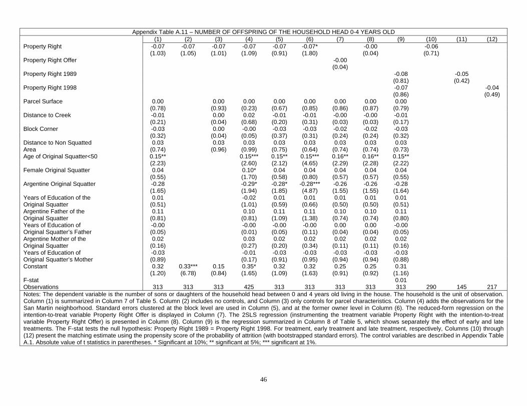
46

Appendix Table A.11 – NUMBER OF OFFSPRING OF THE HOUSEHOLD HEAD 0-4 YEARS OLD (1) (2) (3) (4) (5) (6) (7) (8) (9) (10) (11) (12)

Property Right -0.07 -0.07 -0.07 -0.07 -0.07 -0.07* -0.00 -0.06 (1.03) (1.05) (1.01) (1.09) (0.91) (1.80) (0.04) (0.71) Property Right Offer -0.00 (0.04) Property Right 1989 -0.08 -0.05 (0.81) (0.42) Property Right 1998 -0.07 -0.04 (0.86) (0.49) Parcel Surface 0.00 0.00 0.00 0.00 0.00 0.00 0.00 0.00 (0.78) (0.93) (0.23) (0.67) (0.85) (0.86) (0.87) (0.79) Distance to Creek -0.01 0.00 0.02 -0.01 -0.01 -0.00 -0.00 -0.01 (0.21) (0.04) (0.68) (0.20) (0.31) (0.03) (0.03) (0.17) Block Corner -0.03 0.00 -0.00 -0.03 -0.03 -0.02 -0.02 -0.03 (0.32) (0.04) (0.05) (0.37) (0.31) (0.24) (0.24) (0.32) Distance to Non Squatted 0.03 0.03 0.03 0.03 0.03 0.03 0.03 0.03 Area (0.74) (0.96) (0.99) (0.75) (0.64) (0.74) (0.74) (0.73) Age of Original Squatter<50 0.15** 0.15*** 0.15** 0.15*** 0.16** 0.16** 0.15** (2.23) (2.60) (2.12) (4.65) (2.29) (2.28) (2.22) Female Original Squatter 0.04 0.10* 0.04 0.04 0.04 0.04 0.04 (0.55) (1.70) (0.58) (0.80) (0.57) (0.57) (0.55) Argentine Original Squatter -0.28 -0.29* -0.28* -0.28*** -0.26 -0.26 -0.28 (1.65) (1.94) (1.85) (4.87) (1.55) (1.55) (1.64) Years of Education of the 0.01 -0.02 0.01 0.01 0.01 0.01 0.01 Original Squatter (0.51) (1.01) (0.59) (0.66) (0.50) (0.50) (0.51) Argentine Father of the 0.11 0.10 0.11 0.11 0.10 0.10 0.11 Original Squatter (0.81) (0.81) (1.09) (1.38) (0.74) (0.74) (0.80) Years of Education of -0.00 -0.00 -0.00 -0.00 0.00 0.00 -0.00 Original Squatter’s Father (0.05) (0.01) (0.05) (0.11) (0.04) (0.04) (0.05) Argentine Mother of the 0.02 0.03 0.02 0.02 0.02 0.02 0.02 Original Squatter (0.16) (0.27) (0.20) (0.34) (0.11) (0.11) (0.16) Years of Education of -0.03 -0.01 -0.03 -0.03 -0.03 -0.03 -0.03 Original Squatter’s Mother (0.89) (0.17) (0.91) (0.95) (0.94) (0.94) (0.88) Constant 0.32 0.33*** 0.15 0.35* 0.32 0.32 0.25 0.25 0.31 (1.20) (6.78) (0.84) (1.65) (1.09) (1.63) (0.91) (0.92) (1.16) F-stat 0.01 Observations 313 313 313 425 313 313 313 313 313 290 145 217 Notes: The dependent variable is the number of sons or daughters of the household head between 0 and 4 years old living in the house. The household is the unit of observation. Column (1) is summarized in Column 7 of Table 5. Column (2) includes no controls, and Column (3) only controls for parcel characteristics. Column (4) adds the observations for the San Martin neighborhood. Standard errors clustered at the block level are used in Column (5), and at the former owner level in Column (6). The reduced-form regression on the intention-to-treat variable Property Right Offer is displayed in Column (7). The 2SLS regression (instrumenting the treatment variable Property Right with the intention-to-treat variable Property Right Offer) is presented in Column (8). Column (9) is the regression summarized in Column 8 of Table 5, which shows separately the effect of early and late treatments. The F-stat tests the null hypothesis: Property Right 1989 = Property Right 1998. For treatment, early treatment and late treatment, respectively, Columns (10) through (12) present the matching estimate using the propensity score of the probability of attrition (with bootstrapped standard errors). The control variables are described in Appendix Table A.1. Absolute value of t statistics in parentheses. * Significant at 10%; ** significant at 5%; *** significant at 1%.

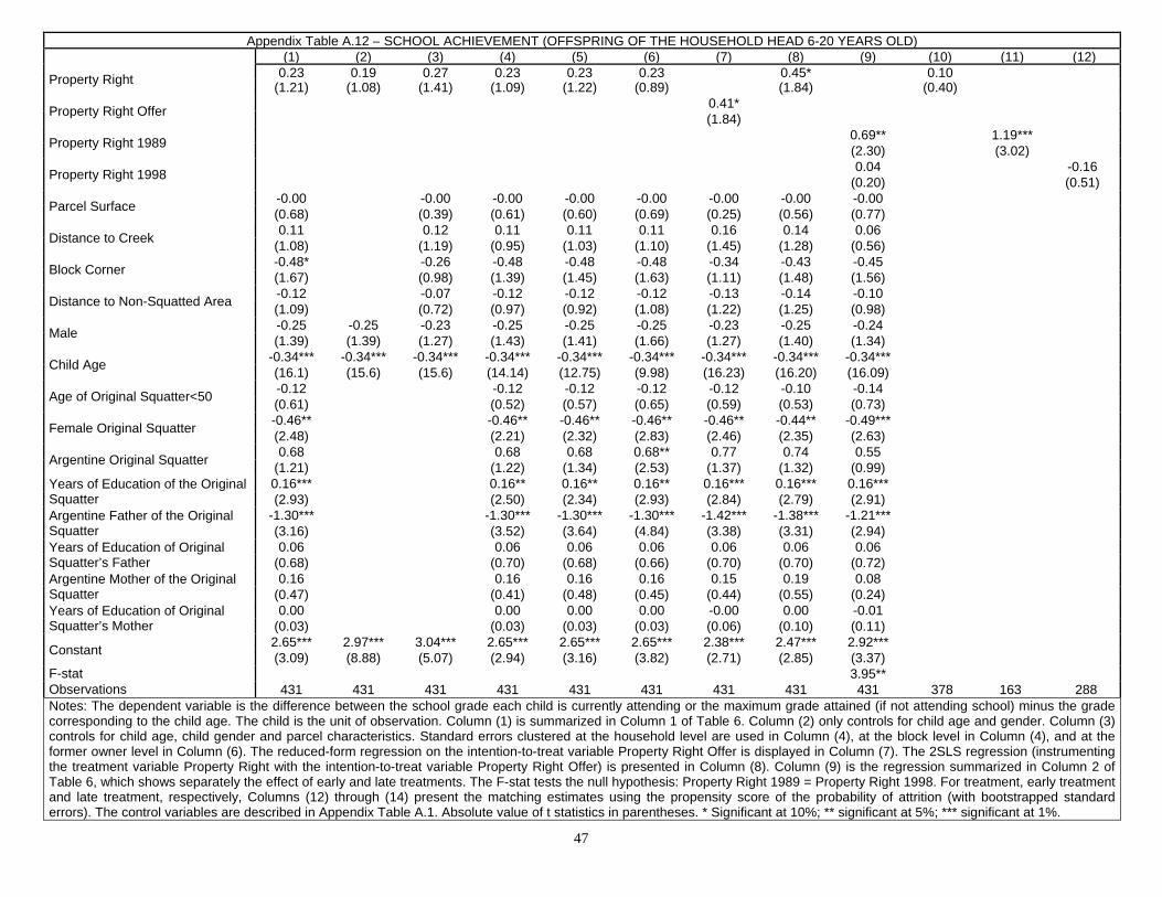
47

Appendix Table A.12 – SCHOOL ACHIEVEMENT (OFFSPRING OF THE HOUSEHOLD HEAD 6-20 YEARS OLD) (1) (2) (3) (4) (5) (6) (7) (8) (9) (10) (11) (12)

0.23 0.19 0.27 0.23 0.23 0.23 0.45* 0.10 Property Right (1.21) (1.08) (1.41) (1.09) (1.22) (0.89) (1.84) (0.40) 0.41* Property Right Offer (1.84) 0.69** 1.19*** Property Right 1989 (2.30) (3.02) 0.04 -0.16 Property Right 1998 (0.20) (0.51)

-0.00 -0.00 -0.00 -0.00 -0.00 -0.00 -0.00 -0.00 Parcel Surface (0.68) (0.39) (0.61) (0.60) (0.69) (0.25) (0.56) (0.77) 0.11 0.12 0.11 0.11 0.11 0.16 0.14 0.06 Distance to Creek (1.08) (1.19) (0.95) (1.03) (1.10) (1.45) (1.28) (0.56)

-0.48* -0.26 -0.48 -0.48 -0.48 -0.34 -0.43 -0.45 Block Corner (1.67) (0.98) (1.39) (1.45) (1.63) (1.11) (1.48) (1.56) -0.12 -0.07 -0.12 -0.12 -0.12 -0.13 -0.14 -0.10 Distance to Non-Squatted Area (1.09) (0.72) (0.97) (0.92) (1.08) (1.22) (1.25) (0.98) -0.25 -0.25 -0.23 -0.25 -0.25 -0.25 -0.23 -0.25 -0.24 Male (1.39) (1.39) (1.27) (1.43) (1.41) (1.66) (1.27) (1.40) (1.34)

-0.34*** -0.34*** -0.34*** -0.34*** -0.34*** -0.34*** -0.34*** -0.34*** -0.34*** Child Age (16.1) (15.6) (15.6) (14.14) (12.75) (9.98) (16.23) (16.20) (16.09) -0.12 -0.12 -0.12 -0.12 -0.12 -0.10 -0.14 Age of Original Squatter<50 (0.61) (0.52) (0.57) (0.65) (0.59) (0.53) (0.73)

-0.46** -0.46** -0.46** -0.46** -0.46** -0.44** -0.49*** Female Original Squatter (2.48) (2.21) (2.32) (2.83) (2.46) (2.35) (2.63) 0.68 0.68 0.68 0.68** 0.77 0.74 0.55 Argentine Original Squatter (1.21) (1.22) (1.34) (2.53) (1.37) (1.32) (0.99)

0.16*** 0.16** 0.16** 0.16** 0.16*** 0.16*** 0.16*** Years of Education of the Original Squatter (2.93) (2.50) (2.34) (2.93) (2.84) (2.79) (2.91)

-1.30*** -1.30*** -1.30*** -1.30*** -1.42*** -1.38*** -1.21*** Argentine Father of the Original Squatter (3.16) (3.52) (3.64) (4.84) (3.38) (3.31) (2.94)

0.06 0.06 0.06 0.06 0.06 0.06 0.06 Years of Education of Original Squatter’s Father (0.68) (0.70) (0.68) (0.66) (0.70) (0.70) (0.72)

0.16 0.16 0.16 0.16 0.15 0.19 0.08 Argentine Mother of the Original Squatter (0.47) (0.41) (0.48) (0.45) (0.44) (0.55) (0.24)

0.00 0.00 0.00 0.00 -0.00 0.00 -0.01 Years of Education of Original Squatter’s Mother (0.03) (0.03) (0.03) (0.03) (0.06) (0.10) (0.11)

2.65*** 2.97*** 3.04*** 2.65*** 2.65*** 2.65*** 2.38*** 2.47*** 2.92*** Constant (3.09) (8.88) (5.07) (2.94) (3.16) (3.82) (2.71) (2.85) (3.37) F-stat 3.95** Observations 431 431 431 431 431 431 431 431 431 378 163 288 Notes: The dependent variable is the difference between the school grade each child is currently attending or the maximum grade attained (if not attending school) minus the grade corresponding to the child age. The child is the unit of observation. Column (1) is summarized in Column 1 of Table 6. Column (2) only controls for child age and gender. Column (3) controls for child age, child gender and parcel characteristics. Standard errors clustered at the household level are used in Column (4), at the block level in Column (4), and at the former owner level in Column (6). The reduced-form regression on the intention-to-treat variable Property Right Offer is displayed in Column (7). The 2SLS regression (instrumenting the treatment variable Property Right with the intention-to-treat variable Property Right Offer) is presented in Column (8). Column (9) is the regression summarized in Column 2 of Table 6, which shows separately the effect of early and late treatments. The F-stat tests the null hypothesis: Property Right 1989 = Property Right 1998. For treatment, early treatment and late treatment, respectively, Columns (12) through (14) present the matching estimates using the propensity score of the probability of attrition (with bootstrapped standard errors). The control variables are described in Appendix Table A.1. Absolute value of t statistics in parentheses. * Significant at 10%; ** significant at 5%; *** significant at 1%.

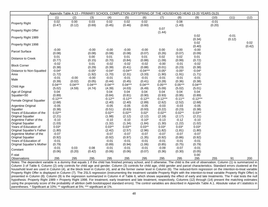
48

Appendix Table A.13 – PRIMARY SCHOOL COMPLETION (OFFSPRING OF THE HOUSEHOLD HEAD 13-20 YEARS OLD)

(1) (2) (3) (4) (5) (6) (7) (8) (9) (10) (11) (12) 0.02 0.00 0.03 0.02 0.02 0.02   0.08   -0.01 Property Right (0.47) (0.12) (0.69) (0.45) (0.46) (0.60)   (1.43)   (0.20)

0.07 Property Right Offer (1.44)   0.02 -0.01 Property Right 1989   (0.34) (0.12)   0.02 0.02 Property Right 1998 (0.40) (0.42)

-0.00 -0.00 -0.00 -0.00 -0.00 0.00 0.00 -0.00 Parcel Surface (0.08) (0.08) (0.08) (0.08) (0.07) (0.26) (0.07) (0.09) 0.01 0.00 0.01 0.01 0.01 0.02 0.02 0.01 Distance to Creek (0.77) (0.15) (0.70) (0.84) (0.88) (1.09) (0.99) (0.72) -0.02 0.01 -0.02 -0.02 -0.02 -0.00 -0.01 -0.02 Block Corner (0.38) (0.29) (0.39) (0.41) (0.88) (0.01) (0.23) (0.38) -0.04* -0.05* -0.04* -0.04** -0.04*** -0.05* -0.05* -0.04* Distance to Non-Squatted

Area (1.72) (1.92) (1.70) (2.31) (3.33) (1.90) (1.91) (1.71) -0.01 -0.00 -0.00 -0.01 -0.01 -0.01 -0.01 -0.01 -0.01 Male (0.39) (0.02) (0.05) (0.44) (0.45) (0.41) (0.28) (0.36) (0.38)

0.04*** 0.04*** 0.04*** 0.04*** 0.04*** 0.04*** 0.05*** 0.05*** 0.04*** Child Age (5.02) (4.59) (4.74) (4.39) (4.03) (6.49) (5.09) (5.02) (5.01) 0.04 0.04 0.04 0.04 0.04 0.04 0.04 Age of Original

Squatter<50 (0.89) (0.84) (0.81) (0.90) (0.93) (0.95) (0.89) -0.12*** -0.12** -0.12** -0.12** -0.12*** -0.11** -0.12*** Female Original Squatter (2.68) (2.40) (2.40) (2.89) (2.62) (2.52) (2.68)

-0.05 -0.05 -0.05 -0.05 -0.03 -0.03 -0.05 Argentine Original Squatter (0.38) (0.51) (0.63) (0.93) (0.22) (0.23) (0.38)

0.02** 0.02** 0.02** 0.02* 0.02** 0.02** 0.03** Years of Education of the Original Squatter (2.21) (1.98) (2.12) (2.12) (2.18) (2.17) (2.21)

-0.10 -0.10 -0.10 -0.10* -0.13 -0.12 -0.10 Argentine Father of the Original Squatter (1.03) (1.32) (1.34) (1.84) (1.30) (1.22) (1.02)

0.03* 0.03** 0.03** 0.03** 0.03* 0.03* 0.03* Years of Education of Original Squatter’s Father (1.80) (2.42) (2.57) (2.96) (1.82) (1.81) (1.80)

-0.07 -0.07 -0.07 -0.07 -0.07 -0.07 -0.07 Argentine Mother of the Original Squatter (0.92) (0.92) (0.97) (1.35) (0.92) (0.86) (0.92)

-0.01 -0.01 -0.01 -0.01 -0.01 -0.01 -0.01 Years of Education of Original Squatter’s Mother (0.79) (0.89) (0.94) (1.06) (0.85) (0.75) (0.79)

-0.01 0.03 0.08 -0.01 -0.01 -0.01 -0.09 -0.07 -0.01 Constant (0.06) (0.20) (0.42) (0.06) (0.06) (0.07) (0.36) (0.30) (0.05) F-stat 0.00 Observations 295 295 295 295 295 295 295 295 295 255 91 200 Notes: The dependent variable is a dummy that equals 1 if the child has finished primary school, and 0 otherwise. The child is the unit of observation. Column (1) is summarized in Column 3 of Table 6. Column (2) only controls for child age and gender. Column (3) controls for child age, child gender and parcel characteristics. Standard errors clustered at the household level are used in Column (4), at the block level in Column (4), and at the former owner level in Column (6). The reduced-form regression on the intention-to-treat variable Property Right Offer is displayed in Column (7). The 2SLS regression (instrumenting the treatment variable Property Right with the intention-to-treat variable Property Right Offer) is presented in Column (8). Column (9) is the regression summarized in Column 4 of Table 6, which shows separately the effect of early and late treatments. The F-stat tests the null hypothesis: Property Right 1989 = Property Right 1998. For treatment, early treatment and late treatment, respectively, Columns (12) through (14) present the matching estimates using the propensity score of the probability of attrition (with bootstrapped standard errors). The control variables are described in Appendix Table A.1. Absolute value of t statistics in parentheses. * Significant at 10%; ** significant at 5%; *** significant at 1%.

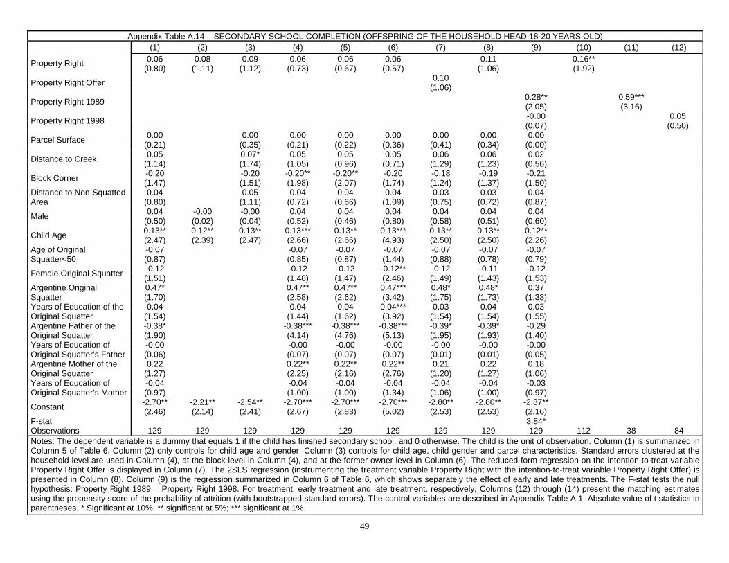
49

Appendix Table A.14 – SECONDARY SCHOOL COMPLETION (OFFSPRING OF THE HOUSEHOLD HEAD 18-20 YEARS OLD)

(1) (2) (3) (4) (5) (6) (7) (8) (9) (10) (11) (12) 0.06 0.08 0.09 0.06 0.06 0.06   0.11   0.16** Property Right (0.80) (1.11) (1.12) (0.73) (0.67) (0.57)   (1.06)   (1.92)

0.10 Property Right Offer (1.06)   0.28** 0.59*** Property Right 1989   (2.05) (3.16)   -0.00 0.05 Property Right 1998 (0.07) (0.50)

0.00 0.00 0.00 0.00 0.00 0.00 0.00 0.00 Parcel Surface (0.21) (0.35) (0.21) (0.22) (0.36) (0.41) (0.34) (0.00) 0.05 0.07* 0.05 0.05 0.05 0.06 0.06 0.02 Distance to Creek (1.14) (1.74) (1.05) (0.96) (0.71) (1.29) (1.23) (0.56) -0.20 -0.20 -0.20** -0.20** -0.20 -0.18 -0.19 -0.21 Block Corner (1.47) (1.51) (1.98) (2.07) (1.74) (1.24) (1.37) (1.50) 0.04 0.05 0.04 0.04 0.04 0.03 0.03 0.04 Distance to Non-Squatted

Area (0.80) (1.11) (0.72) (0.66) (1.09) (0.75) (0.72) (0.87) 0.04 -0.00 -0.00 0.04 0.04 0.04 0.04 0.04 0.04 Male (0.50) (0.02) (0.04) (0.52) (0.46) (0.80) (0.58) (0.51) (0.60)

0.13** 0.12** 0.13** 0.13*** 0.13** 0.13*** 0.13** 0.13** 0.12** Child Age (2.47) (2.39) (2.47) (2.66) (2.66) (4.93) (2.50) (2.50) (2.26) -0.07 -0.07 -0.07 -0.07 -0.07 -0.07 -0.07 Age of Original

Squatter<50 (0.87) (0.85) (0.87) (1.44) (0.88) (0.78) (0.79) -0.12 -0.12 -0.12 -0.12** -0.12 -0.11 -0.12 Female Original Squatter (1.51) (1.48) (1.47) (2.46) (1.49) (1.43) (1.53) 0.47* 0.47** 0.47** 0.47*** 0.48* 0.48* 0.37 Argentine Original

Squatter (1.70) (2.58) (2.62) (3.42) (1.75) (1.73) (1.33) 0.04 0.04 0.04 0.04*** 0.03 0.04 0.03 Years of Education of the

Original Squatter (1.54) (1.44) (1.62) (3.92) (1.54) (1.54) (1.55) -0.38* -0.38*** -0.38*** -0.38*** -0.39* -0.39* -0.29 Argentine Father of the

Original Squatter (1.90) (4.14) (4.76) (5.13) (1.95) (1.93) (1.40) -0.00 -0.00 -0.00 -0.00 -0.00 -0.00 -0.00 Years of Education of

Original Squatter’s Father (0.06) (0.07) (0.07) (0.07) (0.01) (0.01) (0.05) 0.22 0.22** 0.22** 0.22** 0.21 0.22 0.18 Argentine Mother of the

Original Squatter (1.27) (2.25) (2.16) (2.76) (1.20) (1.27) (1.06) -0.04 -0.04 -0.04 -0.04 -0.04 -0.04 -0.03 Years of Education of

Original Squatter’s Mother (0.97) (1.00) (1.00) (1.34) (1.06) (1.00) (0.97) -2.70** -2.21** -2.54** -2.70*** -2.70*** -2.70*** -2.80** -2.80** -2.37** Constant (2.46) (2.14) (2.41) (2.67) (2.83) (5.02) (2.53) (2.53) (2.16)

F-stat 3.84* Observations 129 129 129 129 129 129 129 129 129 112 38 84 Notes: The dependent variable is a dummy that equals 1 if the child has finished secondary school, and 0 otherwise. The child is the unit of observation. Column (1) is summarized in Column 5 of Table 6. Column (2) only controls for child age and gender. Column (3) controls for child age, child gender and parcel characteristics. Standard errors clustered at the household level are used in Column (4), at the block level in Column (4), and at the former owner level in Column (6). The reduced-form regression on the intention-to-treat variable Property Right Offer is displayed in Column (7). The 2SLS regression (instrumenting the treatment variable Property Right with the intention-to-treat variable Property Right Offer) is presented in Column (8). Column (9) is the regression summarized in Column 6 of Table 6, which shows separately the effect of early and late treatments. The F-stat tests the null hypothesis: Property Right 1989 = Property Right 1998. For treatment, early treatment and late treatment, respectively, Columns (12) through (14) present the matching estimates using the propensity score of the probability of attrition (with bootstrapped standard errors). The control variables are described in Appendix Table A.1. Absolute value of t statistics in parentheses. * Significant at 10%; ** significant at 5%; *** significant at 1%.

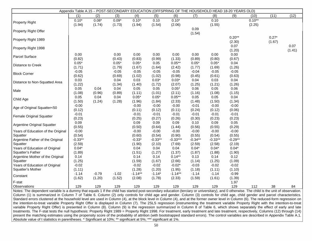
50

Appendix Table A.15 – POST-SECONDARY EDUCATION (OFFSPRING OF THE HOUSEHOLD HEAD 18-20 YEARS OLD) (1) (2) (3) (4) (5) (6) (7) (8) (9) (10) (11) (12)

0.10* 0.08* 0.09* 0.10* 0.10 0.10* 0.10 0.10** Property Right (1.94) (1.74) (1.73) (1.94) (1.54) (2.06) (1.55) (2.25) 0.09 Property Right Offer (1.54) 0.20** 0.27* Property Right 1989 (2.30) (1.67) 0.07 0.07 Property Right 1998 (1.20) (1.41)

0.00 0.00 0.00 0.00 0.00 0.00 0.00 0.00 Parcel Surface (0.82) (0.43) (0.83) (0.99) (1.33) (0.89) (0.80) (0.67) 0.05* 0.05* 0.05* 0.05 0.05** 0.05* 0.05* 0.04 Distance to Creek (1.71) (1.79) (1.67) (1.64) (2.42) (1.77) (1.69) (1.26) -0.05 -0.05 -0.05 -0.05 -0.05 -0.04 -0.05 -0.05 Block Corner (0.62) (0.69) (1.02) (1.02) (0.98) (0.45) (0.61) (0.63) 0.03 0.04 0.03 0.03* 0.03* 0.04 0.03 0.04 Distance to Non-Squatted Area (1.22) (1.34) (1.40) (1.72) (2.07) (1.25) (1.21) (1.26) 0.05 0.04 0.04 0.05 0.05 0.05* 0.06 0.05 0.06 Male (1.08) (0.96) (0.89) (1.11) (1.01) (2.11) (1.16) (1.08) (1.15) 0.05 0.04 0.04 0.05* 0.05* 0.05** 0.05 0.05 0.04 Child Age (1.50) (1.24) (1.28) (1.96) (1.84) (2.33) (1.48) (1.50) (1.34) -0.00 -0.00 -0.00 -0.00 -0.01 -0.00 -0.00 Age of Original Squatter<50 (0.12) (0.11) (0.12) (0.11) (0.24) (0.12) (0.06) -0.01 -0.01 -0.01 -0.01 -0.01 -0.01 -0.01 Female Original Squatter (0.23) (0.25) (0.27) (0.26) (0.30) (0.23) (0.23) 0.09 0.09 0.09 0.09 0.10 0.09 0.05 Argentine Original Squatter (0.55) (0.50) (0.64) (1.44) (0.56) (0.55) (0.29) -0.00 -0.00 -0.00 -0.00 -0.00 -0.00 -0.00 Years of Education of the Original

Squatter (0.54) (0.60) (0.54) (0.90) (0.55) (0.54) (0.55) -0.33** -0.33* -0.33** -0.33*** -0.34** -0.33** -0.29** Argentine Father of the Original

Squatter (2.59) (1.90) (2.10) (7.69) (2.59) (2.58) (2.19) 0.04* 0.04 0.04 0.04 0.04* 0.04* 0.04* Years of Education of Original

Squatter’s Father (1.89) (1.51) (1.27) (1.37) (1.87) (1.88) (1.90) 0.14 0.14 0.14 0.14** 0.13 0.14 0.12 Argentine Mother of the Original

Squatter (1.25) (1.59) (1.67) (2.66) (1.14) (1.25) (1.09) -0.02 -0.02 -0.02 -0.02* -0.03 -0.02 -0.02 Years of Education of Original

Squatter’s Mother (1.11) (1.28) (1.20) (1.95) (1.18) (1.11) (1.10) -1.14 -0.79 -1.02 -1.14** -1.14* -1.14** -1.14 -1.14 -0.99 Constant (1.62) (1.20) (1.52) (2.08) (1.78) (2.33) (1.59) (1.61) (1.39)

F-stat 1.97 Observations 129 129 129 129 129 129 129 129 129 112 38 84 Notes: The dependent variable is a dummy that equals 1 if the child has started post-secondary education (terciary or universitary), and 0 otherwise. The child is the unit of observation. Column (1) is summarized in Column 7 of Table 6. Column (2) only controls for child age and gender. Column (3) controls for child age, child gender and parcel characteristics. Standard errors clustered at the household level are used in Column (4), at the block level in Column (4), and at the former owner level in Column (6). The reduced-form regression on the intention-to-treat variable Property Right Offer is displayed in Column (7). The 2SLS regression (instrumenting the treatment variable Property Right with the intention-to-treat variable Property Right Offer) is presented in Column (8). Column (9) is the regression summarized in Column 8 of Table 6, which shows separately the effect of early and late treatments. The F-stat tests the null hypothesis: Property Right 1989 = Property Right 1998. For treatment, early treatment and late treatment, respectively, Columns (12) through (14) present the matching estimates using the propensity score of the probability of attrition (with bootstrapped standard errors). The control variables are described in Appendix Table A.1. Absolute value of t statistics in parentheses. * Significant at 10%; ** significant at 5%; *** significant at 1%.

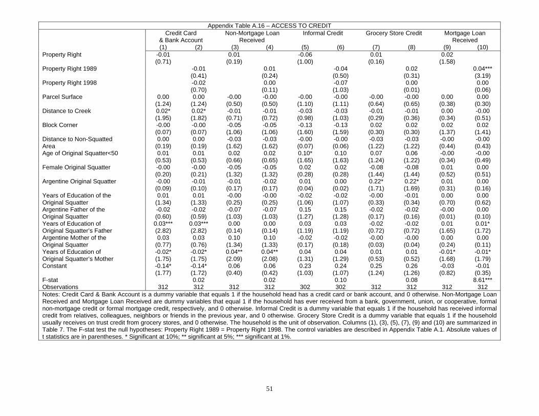
51

Appendix Table A.16 – ACCESS TO CREDIT

Credit Card & Bank Account

Non-Mortgage Loan Received

Informal Credit Grocery Store Credit Mortgage Loan Received

(1) (2) (3) (4) (5) (6) (7) (8) (9) (10) Property Right -0.01 0.01 -0.06 0.01 0.02 (0.71) (0.19) (1.00) (0.16) (1.58) Property Right 1989 -0.01 0.01 -0.04 0.02 0.04*** (0.41) (0.24) (0.50) (0.31) (3.19) Property Right 1998 -0.02 0.00 -0.07 0.00 0.00 (0.70) (0.11) (1.03) (0.01) (0.06) Parcel Surface 0.00 0.00 -0.00 -0.00 -0.00 -0.00 -0.00 -0.00 0.00 0.00 (1.24) (1.24) (0.50) (0.50) (1.10) (1.11) (0.64) (0.65) (0.38) (0.30) Distance to Creek 0.02* 0.02* -0.01 -0.01 -0.03 -0.03 -0.01 -0.01 0.00 -0.00 (1.95) (1.82) (0.71) (0.72) (0.98) (1.03) (0.29) (0.36) (0.34) (0.51) Block Corner -0.00 -0.00 -0.05 -0.05 -0.13 -0.13 0.02 0.02 0.02 0.02 (0.07) (0.07) (1.06) (1.06) (1.60) (1.59) (0.30) (0.30) (1.37) (1.41) Distance to Non-Squatted 0.00 0.00 -0.03 -0.03 -0.00 -0.00 -0.03 -0.03 -0.00 -0.00 Area (0.19) (0.19) (1.62) (1.62) (0.07) (0.06) (1.22) (1.22) (0.44) (0.43) Age of Original Squatter<50 0.01 0.01 0.02 0.02 0.10* 0.10 0.07 0.06 -0.00 -0.00 (0.53) (0.53) (0.66) (0.65) (1.65) (1.63) (1.24) (1.22) (0.34) (0.49) Female Original Squatter -0.00 -0.00 -0.05 -0.05 0.02 0.02 -0.08 -0.08 0.01 0.00 (0.20) (0.21) (1.32) (1.32) (0.28) (0.28) (1.44) (1.44) (0.52) (0.51) Argentine Original Squatter -0.00 -0.01 -0.01 -0.02 0.01 0.00 0.22* 0.22* 0.01 0.00 (0.09) (0.10) (0.17) (0.17) (0.04) (0.02) (1.71) (1.69) (0.31) (0.16) Years of Education of the 0.01 0.01 -0.00 -0.00 -0.02 -0.02 -0.00 -0.01 0.00 0.00 Original Squatter (1.34) (1.33) (0.25) (0.25) (1.06) (1.07) (0.33) (0.34) (0.70) (0.62) Argentine Father of the -0.02 -0.02 -0.07 -0.07 0.15 0.15 -0.02 -0.02 -0.00 0.00 Original Squatter (0.60) (0.59) (1.03) (1.03) (1.27) (1.28) (0.17) (0.16) (0.01) (0.10) Years of Education of 0.03*** 0.03*** 0.00 0.00 0.03 0.03 -0.02 -0.02 0.01 0.01* Original Squatter’s Father (2.82) (2.82) (0.14) (0.14) (1.19) (1.19) (0.72) (0.72) (1.65) (1.72) Argentine Mother of the 0.03 0.03 0.10 0.10 -0.02 -0.02 -0.00 -0.00 0.00 0.00 Original Squatter (0.77) (0.76) (1.34) (1.33) (0.17) (0.18) (0.03) (0.04) (0.24) (0.11) Years of Education of -0.02* -0.02* 0.04** 0.04** 0.04 0.04 0.01 0.01 -0.01* -0.01* Original Squatter’s Mother (1.75) (1.75) (2.09) (2.08) (1.31) (1.29) (0.53) (0.52) (1.68) (1.79) Constant -0.14* -0.14* 0.06 0.06 0.23 0.24 0.25 0.26 -0.03 -0.01 (1.77) (1.72) (0.40) (0.42) (1.03) (1.07) (1.24) (1.26) (0.82) (0.35) F-stat 0.02 0.02 0.10 0.08 8.61*** Observations 312 312 312 312 302 302 312 312 312 312 Notes: Credit Card & Bank Account is a dummy variable that equals 1 if the household head has a credit card or bank account, and 0 otherwise. Non-Mortgage Loan Received and Mortgage Loan Received are dummy variables that equal 1 if the household has ever received from a bank, government, union, or cooperative, formal non-mortgage credit or formal mortgage credit, respectively, and 0 otherwise. Informal Credit is a dummy variable that equals 1 if the household has received informal credit from relatives, colleagues, neighbors or friends in the previous year, and 0 otherwise. Grocery Store Credit is a dummy variable that equals 1 if the household usually receives on trust credit from grocery stores, and 0 otherwise. The household is the unit of observation. Columns (1), (3), (5), (7), (9) and (10) are summarized in Table 7. The F-stat test the null hypotheses: Property Right 1989 = Property Right 1998. The control variables are described in Appendix Table A.1. Absolute values of t statistics are in parentheses. * Significant at 10%; ** significant at 5%; *** significant at 1%.

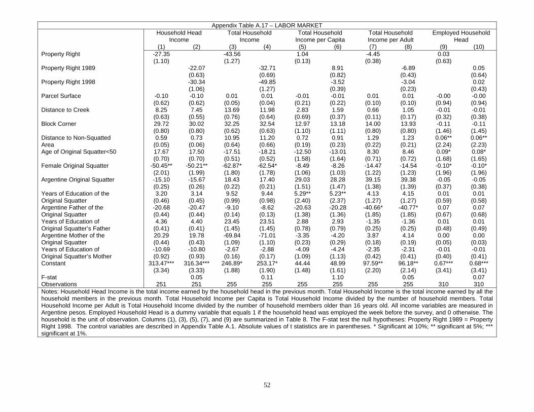
52

Appendix Table A.17 – LABOR MARKET

Household Head Income

Total Household Income

Total Household Income per Capita

Total Household Income per Adult

Employed Household Head

(1) (2) (3) (4) (5) (6) (7) (8) (9) (10) Property Right -27.35 -43.56 1.04 -4.45 0.03 (1.10) (1.27) (0.13) (0.38) (0.63) Property Right 1989 -22.07 -32.71 8.91 -6.89 0.05 (0.63) (0.69) (0.82) (0.43) (0.64) Property Right 1998 -30.34 -49.85 -3.52 -3.04 0.02 (1.06) (1.27) (0.39) (0.23) (0.43) Parcel Surface -0.10 -0.10 0.01 0.01 -0.01 -0.01 0.01 0.01 -0.00 -0.00 (0.62) (0.62) (0.05) (0.04) (0.21) (0.22) (0.10) (0.10) (0.94) (0.94) Distance to Creek 8.25 7.45 13.69 11.98 2.83 1.59 0.66 1.05 -0.01 -0.01 (0.63) (0.55) (0.76) (0.64) (0.69) (0.37) (0.11) (0.17) (0.32) (0.38) Block Corner 29.72 30.02 32.25 32.54 12.97 13.18 14.00 13.93 -0.11 -0.11 (0.80) (0.80) (0.62) (0.63) (1.10) (1.11) (0.80) (0.80) (1.46) (1.45) Distance to Non-Squatted 0.59 0.73 10.95 11.20 0.72 0.91 1.29 1.23 0.06** 0.06** Area (0.05) (0.06) (0.64) (0.66) (0.19) (0.23) (0.22) (0.21) (2.24) (2.23) Age of Original Squatter<50 17.67 17.50 -17.51 -18.21 -12.50 -13.01 8.30 8.46 0.09* 0.08* (0.70) (0.70) (0.51) (0.52) (1.58) (1.64) (0.71) (0.72) (1.68) (1.65) Female Original Squatter -50.45** -50.21** -62.87* -62.54* -8.49 -8.26 -14.47 -14.54 -0.10* -0.10* (2.01) (1.99) (1.80) (1.78) (1.06) (1.03) (1.22) (1.23) (1.96) (1.96) Argentine Original Squatter -15.10 -15.67 18.43 17.40 29.03 28.28 39.15 39.38 -0.05 -0.05 (0.25) (0.26) (0.22) (0.21) (1.51) (1.47) (1.38) (1.39) (0.37) (0.38) Years of Education of the 3.20 3.14 9.52 9.44 5.29** 5.23** 4.13 4.15 0.01 0.01 Original Squatter (0.46) (0.45) (0.99) (0.98) (2.40) (2.37) (1.27) (1.27) (0.59) (0.58) Argentine Father of the -20.68 -20.47 -9.10 -8.62 -20.63 -20.28 -40.66* -40.77* 0.07 0.07 Original Squatter (0.44) (0.44) (0.14) (0.13) (1.38) (1.36) (1.85) (1.85) (0.67) (0.68) Years of Education of 4.36 4.40 23.45 23.51 2.88 2.93 -1.35 -1.36 0.01 0.01 Original Squatter’s Father (0.41) (0.41) (1.45) (1.45) (0.78) (0.79) (0.25) (0.25) (0.48) (0.49) Argentine Mother of the 20.29 19.78 -69.84 -71.01 -3.35 -4.20 3.87 4.14 0.00 0.00 Original Squatter (0.44) (0.43) (1.09) (1.10) (0.23) (0.29) (0.18) (0.19) (0.05) (0.03) Years of Education of -10.69 -10.80 -2.67 -2.88 -4.09 -4.24 -2.35 -2.31 -0.01 -0.01 Original Squatter’s Mother (0.92) (0.93) (0.16) (0.17) (1.09) (1.13) (0.42) (0.41) (0.40) (0.41) Constant 313.47*** 316.34*** 246.89* 253.17* 44.44 48.99 97.59** 96.18** 0.67*** 0.68*** (3.34) (3.33) (1.88) (1.90) (1.48) (1.61) (2.20) (2.14) (3.41) (3.41) F-stat 0.05 0.11 1.10 0.05 0.07 Observations 251 251 255 255 255 255 255 255 310 310 Notes: Household Head Income is the total income earned by the household head in the previous month. Total Household Income is the total income earned by all the household members in the previous month. Total Household Income per Capita is Total Household Income divided by the number of household members. Total Household Income per Adult is Total Household Income divided by the number of household members older than 16 years old. All income variables are measured in Argentine pesos. Employed Household Head is a dummy variable that equals 1 if the household head was employed the week before the survey, and 0 otherwise. The household is the unit of observation. Columns (1), (3), (5), (7), and (9) are summarized in Table 8. The F-stat test the null hypotheses: Property Right 1989 = Property Right 1998. The control variables are described in Appendix Table A.1. Absolute values of t statistics are in parentheses. * Significant at 10%; ** significant at 5%; *** significant at 1%.