Embed Size (px)
Citation preview

HAL Id: tel-03351962https://tel.archives-ouvertes.fr/tel-03351962v2
Submitted on 22 Sep 2021
HAL is a multi-disciplinary open accessarchive for the deposit and dissemination of sci-entific research documents, whether they are pub-lished or not. The documents may come fromteaching and research institutions in France orabroad, or from public or private research centers.
L’archive ouverte pluridisciplinaire HAL, estdestinée au dépôt et à la diffusion de documentsscientifiques de niveau recherche, publiés ou non,émanant des établissements d’enseignement et derecherche français ou étrangers, des laboratoirespublics ou privés.
Proportional-Fair Scheduling of Mobile Users based on aPartial View of Future Channel Conditions
Thi Thuy Nga Nguyen
To cite this version:Thi Thuy Nga Nguyen. Proportional-Fair Scheduling of Mobile Users based on a Partial View ofFuture Channel Conditions. Automatic Control Engineering. INSA de Toulouse, 2020. English.�NNT : 2020ISAT0023�. �tel-03351962v2�

THÈSEEn vue de l’obtention du
DOCTORAT DE L’UNIVERSITÉ DE TOULOUSE
Délivré par l'Institut National des Sciences Appliquées deToulouse
Présentée et soutenue par
Thi Thuy Nga NGUYEN
Le 30 novembre 2020
Ordonnancement garantissant l'équité proportionnelle desutilisateurs mobiles basé sur une connaissance partielle des
conditions futures des canaux
Ecole doctorale : SYSTEMES
Spécialité : Automatique et Informatique
Unité de recherche :LAAS - Laboratoire d'Analyse et d'Architecture des Systèmes
Thèse dirigée parOlivier BRUN et Balakrishna PRABHU
Jury
Olivier BRUN, Directeur de ThèseM. lain PIROVANO, ExaminateurM.A
Mme Isabel AMIGO, ExaminatriceMme Hind CASTEL, Rapporteure
Rachid ELAZOUZI, Rapporteur M.
Balakrishna PRABHU, Co-directeur de thèseM.
M. Bruno COUDOIN, invité

Acknowledgments
I would like to take this opportunity to say thank so much to my two supervi-sors, Bala and Olivier, for their guidance during my thesis. Thank so much Mr.Bruno Coudoin for his help during the past three years. Thank very much themembers of my thesis committee for spending their time reading the manuscriptand giving me many useful comments. Thank a lot and again Bala, for manythings he helped me, I am grateful to him.
I would like to say sincerely thank to my friends and my colleges at LAAS, atTorus Actions and from many place in France and in Vietnam for their support,not only in studying but also in many other aspects of life.
Thank my family, my parents and my two sisters, who constantly supportme and always believe in me for whatever I choose.
Thank the professors at Institute of Mathematics, Vietnam academy of sci-ence and technology for their support and giving me the chance to start myjourney in France.
Thank Urtzi for his guidance when I started working on applied mathematicsdomain and partially helping me do the first paper I have ever done.
Also, I would like to thank Continental Digital service in France and LAAS-CNRS for giving me this great opportunity.
Toulouse, 30 November 2020

0.1. ABSTRACT - FRENCH VERSION 3
0.1 Abstract - French Version
Dans les reseaux de communication, un ordonnanceur decide quelles ressourcesdoit etre attribuee a quel utilisateur. Les ressources disponibles etant limiteeset les besoins des utilisateurs etant heterogenes, le choix de l’ordonnanceurjoue un role important dans la conception du reseau. Avec l’augmentation dela demande en ressources reseaux, due a l’utilisation croissante d’appareilsmobiles et notamment a l’emergence des vehicules connectes, ce problemed’ordonnancement devient a la fois plus critique et plus complexe. Les or-donnanceurs utilises actuellement allouent le canal en considerant son etatactuel, et eventuellement ses etats passes, mais sans tenir compte de ses etatsfuturs. Ceci conduit a une allocation sous-optimale des ressources, ce quipeux avoir un effet nefaste sur les performances du reseau dans les periodesde congestion. Dans cette these, nous proposons un ensemble d’algorithmesd’ordonnancement qui exploitent l’information sur les etats futurs du canalpour ameliorer l’utilite totale du reseau. Le premier ensemble d’algorithmesest concu comme une amelioration de l’ordonnanceur a equite proportion-nelle dont l’objectif est de maintenir un certain equilibre entre d’une part undebit total eleve et d’autre part une certaine equite entre utilisateurs garan-tissant a chacun un niveau proportionnelle de service. Le deuxieme ensembled’algorithmes effectuent conjointement controle de puissance et allocation ducanal, toujours dans le but de maximiser une fonction d’utilite basee sur leconcept d’equite proportionnelle. Les experiences numeriques realisees avecdes modeles simples de mobilite ainsi qu’avec des traces generees en utilisantl’environnement SUMO montrent que les algorithmes proposes ameliorentl’utilite, a la fois lorsque le reseau comporte une seule station de base etlorsqu’il en comporte plusieurs. Un des inconvenients des algorithmes pro-poses est qu’a chaque instant de decision il est necessaire de resoudre unprobleme d’optimisation convexe de grande dimension, ce qui peut etre redhi-bitoire pour certains scenarios. C’est pourquoi, dans la derniere partie de lathese, nous explorons une methode basee sur un reseau de neurones profondpour apprendre les decisions des algorithmes proposes. Cette methode per-met de generer des decisions beaucoup plus rapidement tout en ayant unefaible erreur d’approximation.

4
0.2 Abstract - English Version
In communication networks, a scheduler decides which network resources areallocated to which user. Due to limited available resources and heteroge-neous user requirements, the choice of the scheduler plays an important rolein network design. The increasing use of mobile devices, and in particularconnected vehicles, is expected to drive the demand for network resourceseven higher making the scheduling problem more critical and complex. Thecurrent generation of schedulers base their decisions mainly on the past andthe current channel state information but do not take into account the fu-ture channel state information. This leads to a sub-optimal allocation ofresources which can then have a significant and adverse impact on networkperformance during periods of saturation. In this thesis, we propose a setof scheduling algorithms based on future channel state information with theobjective of improving the total network utility. The first set of algorithmsare designed as an improvement to the proportional fair scheduler whose ob-jective is to maintain the balance between getting high total throughput andguarantee everyone getting a proportionally level of service. The second setof algorithms perform joint power control and channel allocation again withthe objective of maximizing the proportional fair utility. Numerical exper-iments conducted with simple mobility models as well as traces generatedusing the SUMO mobility environment show that the proposed algorithmsimprove the utility in both single and multi-base stations networks. One ofthe downside is that, at each decision instant, the proposed algorithms needto solve a high dimensional convex optimization problem that may be com-putationally prohibitive in some real-time scenarios. In the final part of thethesis, we explore a deep neural network based method to learn the decisionsof the proposed algorithms. This method is able to generate decisions muchfaster while maintaining a low approximation error.

Contents
0.1 Abstract - French Version . . . . . . . . . . . . . . . . . . . . 30.2 Abstract - English Version . . . . . . . . . . . . . . . . . . . . 4
1 Introduction 91.1 Motivation of the thesis . . . . . . . . . . . . . . . . . . . . . 91.2 Problems addressed in the thesis . . . . . . . . . . . . . . . . . 101.3 Thesis contributions . . . . . . . . . . . . . . . . . . . . . . . 101.4 Thesis organization . . . . . . . . . . . . . . . . . . . . . . . . 11
2 Background 132.1 Connected Vehicle Technology . . . . . . . . . . . . . . . . . . 13
2.1.1 eHorizon project by Continental Digital Service in France 142.2 Wireless connectivity solutions . . . . . . . . . . . . . . . . . . 152.3 Basics concepts . . . . . . . . . . . . . . . . . . . . . . . . . . 16
2.3.1 Channel Capacity and Signal-to-noise ratio (SNR) . . . 162.3.2 Fading effects . . . . . . . . . . . . . . . . . . . . . . . 162.3.3 Data rate, Throughput . . . . . . . . . . . . . . . . . . 172.3.4 Maximum Utility and Generally Fair Scheduling Problem 17
2.4 Channel Allocation and Power Control . . . . . . . . . . . . . 212.4.1 Some proposed problems in scheduling . . . . . . . . . 212.4.2 Models and Methods proposed in Scheduling . . . . . . 23
2.5 Technical parts . . . . . . . . . . . . . . . . . . . . . . . . . . 252.5.1 KKT conditions for solution of Convex Optimization
Problem . . . . . . . . . . . . . . . . . . . . . . . . . . 252.5.2 Supervised learning with Deep Feedforward Neural Net-
works . . . . . . . . . . . . . . . . . . . . . . . . . . . 262.5.3 Deep Reinforcement Learning by Modeling as a Markov
Decision Process (MDP) . . . . . . . . . . . . . . . . . 28
3 Channel allocation 333.1 Introduction . . . . . . . . . . . . . . . . . . . . . . . . . . . . 34
3.1.1 Contributions . . . . . . . . . . . . . . . . . . . . . . . 36
5

6 CONTENTS
3.1.2 Organisation . . . . . . . . . . . . . . . . . . . . . . . 363.2 Background . . . . . . . . . . . . . . . . . . . . . . . . . . . . 37
3.2.1 Projection on simplex . . . . . . . . . . . . . . . . . . 373.2.2 Projection on feasible set D . . . . . . . . . . . . . . . 37
3.3 Problem formulation . . . . . . . . . . . . . . . . . . . . . . . 383.4 Existing Algorithms . . . . . . . . . . . . . . . . . . . . . . . . 40
3.4.1 Greedy allocation . . . . . . . . . . . . . . . . . . . . . 403.4.2 Proportional Fair (PF) allocation . . . . . . . . . . . . 403.4.3 Predictive Finite-horizon PF Scheduling ((PF)2S) . . . 40
3.5 Projected gradient approach . . . . . . . . . . . . . . . . . . . 423.5.1 Projected gradient short term objective algorithm (STO1) 453.5.2 Projected gradient short term objective algorithm 2
(STO2) . . . . . . . . . . . . . . . . . . . . . . . . . . 463.6 Numerical results . . . . . . . . . . . . . . . . . . . . . . . . . 47
3.6.1 One road network . . . . . . . . . . . . . . . . . . . . . 473.6.2 Network simulation with SUMO . . . . . . . . . . . . . 50
3.7 Summary . . . . . . . . . . . . . . . . . . . . . . . . . . . . . 52
4 Joint power control and channel allocation 574.1 Introduction . . . . . . . . . . . . . . . . . . . . . . . . . . . . 58
4.1.1 Contributions . . . . . . . . . . . . . . . . . . . . . . . 594.1.2 Related work . . . . . . . . . . . . . . . . . . . . . . . 59
4.2 Problem formulation . . . . . . . . . . . . . . . . . . . . . . . 604.2.1 Channel gains . . . . . . . . . . . . . . . . . . . . . . . 62
4.3 Algorithms . . . . . . . . . . . . . . . . . . . . . . . . . . . . . 624.3.1 Locally optimal algorithm . . . . . . . . . . . . . . . . 634.3.2 Short-term Objective 1 (STO1) . . . . . . . . . . . . . 634.3.3 Short-term Objective 2 (STO2) . . . . . . . . . . . . . 65
4.4 Numerical experiments . . . . . . . . . . . . . . . . . . . . . . 664.4.1 Stationary channel . . . . . . . . . . . . . . . . . . . . 664.4.2 Slowly varying channel . . . . . . . . . . . . . . . . . . 674.4.3 Mobility Model . . . . . . . . . . . . . . . . . . . . . . 68
4.5 Summary . . . . . . . . . . . . . . . . . . . . . . . . . . . . . 71
5 Learning the channel allocation algorithm 755.1 Abstract . . . . . . . . . . . . . . . . . . . . . . . . . . . . . . 755.2 Introduction . . . . . . . . . . . . . . . . . . . . . . . . . . . . 75
5.2.1 Related works . . . . . . . . . . . . . . . . . . . . . . . 765.2.2 Contributions . . . . . . . . . . . . . . . . . . . . . . . 775.2.3 Organization . . . . . . . . . . . . . . . . . . . . . . . 77
5.3 Problem Formulation . . . . . . . . . . . . . . . . . . . . . . . 78

CONTENTS 7
5.3.1 Optimization problem and the STO1 algorithm . . . . 785.3.2 Learning STO1 with DFNN . . . . . . . . . . . . . . . 81
5.4 System Setup for learning . . . . . . . . . . . . . . . . . . . . 835.4.1 State . . . . . . . . . . . . . . . . . . . . . . . . . . . . 845.4.2 Target . . . . . . . . . . . . . . . . . . . . . . . . . . . 84
5.5 Discussion about the continuity of the STO1 function . . . . . 855.5.1 Learning with the dual value . . . . . . . . . . . . . . . 915.5.2 Example in a small dimension . . . . . . . . . . . . . . 915.5.3 Proposed method to obtain a continuous function . . . 985.5.4 Loss, DFNN architecture, initial parameters and opti-
mizer . . . . . . . . . . . . . . . . . . . . . . . . . . . . 985.6 Numerical Comparisons . . . . . . . . . . . . . . . . . . . . . 99
5.6.1 An Unified Data Generator for Comparison . . . . . . 995.6.2 Comparison of different DFNN architectures . . . . . . 995.6.3 Comparisons of different loss functions . . . . . . . . . 1055.6.4 Comparisons of different ordering schemes . . . . . . . 1055.6.5 Comparisons of learning the channel allocation against
learning dual values . . . . . . . . . . . . . . . . . . . . 1055.7 Computing times . . . . . . . . . . . . . . . . . . . . . . . . . 1085.8 Discussion on a reinforcement learning based approach for
learning Optimal Policy . . . . . . . . . . . . . . . . . . . . . 1095.9 Summary and Discussion . . . . . . . . . . . . . . . . . . . . . 112
6 Discussion and Future Works 115

8 CONTENTS

Chapter 1
Introduction
1.1 Motivation of the thesis
When a connected vehicle moves on the road, it needs internet connectivityfor exchanging a high volume of information for services such as security,driving conditions, local information, infotainment, etc. Due to mobility,wireless connectivity is the only communication solution that is possible.Compared to wireline networks, wireless resources are much more scarceand expensive which makes resource allocation decisions more important inwireless networks, especially for vehicular networks.
In cellular networks, proportional fairness is the de-facto standard cri-terion that guarantees each user a proportional level of service while main-taining a high system throughput. Recently in 3G and 4G networks, oppor-tunistic schedulers have been incorporated in order to maximize proportionalfairness [12]. Proportional fair (PF) scheduling algorithms [37] are typicalin those opportunistic schedulers. The PF algorithm allocates resources tousers based on current and past information and has been proven asymptot-ically optimal when the wireless channel follows a stationary process and thesojourn time of users are long. However, those assumptions do not neces-sarily hold for vehicular traffic where the channel state is not stationary dueto mobility and the sojourn time is not enough long to get asymptoticallyproperty. Therefore, PF algorithms are not necessary optimized for vehicularsystems.
With the connected vehicle technology [25, 30, 71], future information canbe accessed to improve efficiency of the schedulers, since the more informationwe have, the better the scheduling decisions that can be made. One of themain difficulty for wireless scheduling is that the exact data rate of a wirelesslink can be very difficult to predict even on short-time scales due to various
9

10 CHAPTER 1. INTRODUCTION
phenomenon (fading, shadowing, e.g.) that are specific to wireless networks.However, it is possible to obtain a partial information on the future channelconditions in the form of estimations. For example, the future positions ofa user can be predicted over a short time period if the user accepts to shareinformation about his travel itinerary. Another possibility for estimating thefuture positions of a user is to compute his most probable path by combiningup-to-date information on road traffic conditions with historical data on pasttravel itineraries of the user [36, 31]. Position of the users may not give theexact data rate, but still it can be useful in the sense that if a user is farfrom the Base Station (BS), he should get a lower data rate and converselyif he is close to the BS, he should get a higher rate with a high probability.In this thesis, we shall assume that the mean of channel gains, or the meandata rate can be obtained thanks to users’ predicted future paths.
1.2 Problems addressed in the thesis
In this thesis, we consider two scheduling problems for vehicular systems.The first problem is channel allocation, and the second one is a joint problemof channel allocation and power control. Both problems share the sameobjective which is to maximize the proportional fairness between users. Weshall assume that the future positions of the users are predicted over a shorttime period (some next seconds) and from that we assume the means of futuredata rates (or means of future channel gains) are known for that period. Wetake that partial information on the future channel condition into account toimprove allocation decisions.
1.3 Thesis contributions
The contributions of this thesis can be divided into three main parts whichare presented in three chapters: Chapter 3 which is based on [51], Chapter4 which is based on [52] and Chapter 5.
The first part of the contributions, which is presented in Chapter 3, dealswith channel allocation for improving the proportional fairness between usersusing partial knowledge on future channel condition. In more details, we as-sume that the future positions of moving users are predictable over the nextfew seconds. Combining the positions with the Signal-to-Noise-Ratio (SNR)maps, the mean of future data rates can be computed. We present twoheuristics using the short-time future information to improve fairness utility.We also propose an idea that mixes two types of time scaling to reduce the

1.4. THESIS ORGANIZATION 11
dimension of the original optimization problme. We then compare the per-formance of the two heuristics against other existing algorithms using SUMOwhich is an open-source road traffic simulator. The simulation results showthat the heuristics outperform other algorithms. However, the computationtimes of the heuristics are quite heavy comparing to the other algorithmssince they require solving a convex optimization problem frequently.
The second contribution, which is discussed in Chapter 4, concerns ajoint problem of channel allocation and power control. Again based on apartial view of future channel conditions, we propose two heuristics whichare based on those proposed in 3. We then evaluate the heuristics on threetypes of model: stationary channel gains with fixed mean, slowly-varyingchannel gains and mobility model where the channel gains vary in everychannel allocation slot. For the above three models, the heuristics are shownto outperform the other existing algorithms in which future information isnot available. However, the same problem of high computational times forone of the heuristics forces us to omit it out from numerical evaluations formobility model.
The last part of the contributions is presented in Chapter 5 in whichwe propose using a machine learning based method, and more specifically aDeep Feedforward Neural Network (DFNN), to learn one of the allocationheuristics (the STO1 heuristic, the one that requires more computationaltime) in order to have an approximate algorithm which is many times faster.A Deep Feedforward Neural Network (DFNN) can approximate a continu-ous function with low error, but we provide a counter-example proving thatunfortunately STO1 is not continuous. We then characterize the set of alldiscontinuities, and propose several ordering schemes to reduce the impactof these discontinuities on the learning time. Numerical results show thatthe proposed ordering schemes enable to converge faster. Although STO1 isnot continuous, we show that the dual values of the problem are continuouswith the input features. We thus propose learning the dual values instead ofthe primal ones. Numerical results shows learning with dual values is faster.
1.4 Thesis organization
In Chapter 2, we provide background material on resource allocation in wire-less network. That includes connected vehicle technology, basics conceptsfor scheduling and resource allocation in wireless networks (SNR, Shannonchannel capacity, fading effects, data rate, throughput, fairness, utility maxi-mization, etc.). In addition to a short reminder about the mathematical toolsused in this thesis (Deep Feed-forward neural networks, KKT condition, etc),

12 CHAPTER 1. INTRODUCTION
we also present a short review of previous works on channel allocation andpower control, including potential methods and explanation for why we useor not use them.
In Chapter 3, we consider channel allocation problem for vehicular net-works in a multiple BS setting. In that chapter, we first state the assumptionsand define the objective function. We then discuss some existing algorithmsthat we shall use for comparison. After that we present our heuristic algo-rithms that use a partial view of future channel information for improvedproportional-fair utility. Finally, we employ SUMO for evaluation of theheuristics and the existing algorithms.
In Chapter 4, we consider the joint channel allocation and power controlproblem for a single BS in three settings: stationary channel, slower time scalevarying channel and mobility model where the channel gains vary at a fastertime scale. We first state the problem and assumptions, and then present anexisting algorithm that does not take future information into account. Wethen describe our heuristic algorithms that use future information to improveproportional-fair utility. The numerical comparisons for the three settings forboth existing and heuristics are shown at the end.
In Chapter 5, we present a supervised learning based method for learningone of our heuristic algorithms. We first recall the resource allocation prob-lem that we consider in Chapter 3 in a single BS case, then we recall STO1algorithm and state the learning problem that we want to do in this chap-ter. We define input-output for the DFNN model, then discuss about thecontinuity of that setting and how to reduce discontinuity. Numerical resultsare shown after that. At the end we discuss several research directions thatcan be done in the future including a reinforcement learning based approach,that we did not succeed in but is nevertheless interesting to discuss.
Finally, some conclusions are drawn in Chapter 6, where we also discusspossible extensions of this work and future research directions.

Chapter 2
Background material
2.1 Connected Vehicle Technology
Connected vehicle technology enables vehicles and infrastructures to com-municate and share transportation information using wireless technology.Thanks to a high-speed wireless connection, a connected car can carry on-board many applications to improve traffic safety, security and comfort (suchas infotainment, parking assistance).
The connected vehicle concept refers to not only the vehicles and theinfrastructure but also to applications, services, and technologies that enablea vehicle to interact with its environment.
There are five ways a vehicle can connect to the surroundings and com-municate with them:
• connecting to the infrastructure (V2I), which lets the vehicle be awareof the infrastructure surrounding it and also lets the infrastructureobtain information from the vehicle.
• communicating between vehicles (V2V), the purpose of this is to shareinformation about speed, position, etc. between neighbouring vehiclesin order to reduce congestion, avoid accidents and increase positiveimpact on the surroundings.
• exchanging information with the Cloud (V2C), this allows the vehicleto exchange information about and for applications (such as drivingassistance, infotainment, and vehicle maintenance).
• communicating with personal mobile devices with the Pedestrian (V2P)to perceive the environment in order to improve safety and mobility.
13

14 CHAPTER 2. BACKGROUND
• interconnecting with Everything (V2X) including other connected ve-hicles, infrastructure and personal mobile devices.
Such types of connectivity help a connected vehicle and the system bebetter aware of each other and of the surroundings in order to have moreintelligent decision during its mobility.
2.1.1 eHorizon project by Continental Digital Servicein France
Electronic Horizon is an embedded software for cloud-based virtual sensornetwork for exchanging detailed road network information (map data, vehi-cle’s mobility model and the road ahead) between the cloud and the vehiclesto help the vehicle make intelligent decisions. It has been a subject of severalacademic papers [25], [30],[71] and practical tests [1].
With the Electronic Horizon project (eHorizon), Continental wants tomake mobility safer, proper and smarter. Continental perceives digital trans-formation as a tremendous lever to strengthen its contribution to these threeobjectives. This relates to the transformation of the manufacturing and useof automotive systems, but beyond the whole mobility experience.
Continental Digital Services France1 (CDSF) is a new subsidiary of Con-tinental Automotive France which was created to address these opportunitiesaround connected vehicles, autonomous vehicles and mobility services. Thegoal is to merge on-board intelligence with that of the in-house platform”in-the-cloud”. For each connected vehicle, a cloud assistant can access in-formation in real time far beyond the horizon of its on-board sensors. Ona larger scale, it makes possible global analysis on the history of movementflows of all vehicles, while preserving user confidentiality.
The new services considered in the eHorizon project of the automotivesupplier Continental thus integrate ever more numerous and important inter-actions between vehicles that have become connected and their environment.These new interactions will link various pieces of equipment in the vehicle,and in particular important components for passenger safety such as brakes,steering or obstacle detection radars, with signaling elements (traffic lights,solid lines non-crossing, level crossings, etc.) or other users of the trafficnetwork (other vehicles, cyclist, pedestrians, speed bump, etc.).
Among the new services, some, such as engine monitoring or increasedvisibility, will be critical. However, they will have to share the available
1This thesis is supported by a contract with Continental Digital Services in France.It is in the eHorizon project which is about connected vehicles, autonomous vehicles andmobility services.

2.2. WIRELESS CONNECTIVITY SOLUTIONS 15
bandwidth with non-critical applications such as multimedia and infotain-ment. By definition, critical services require a higher quality of service thannon-critical services for whom the quality can be adjusted according to thecircumstances. A vehicle will be driven in very varied environments - urbanenvironment, traffic jams, highways, tunnels, remote areas. Each of these en-vironments has a different effect on the quality of communication between thevehicle and the infrastructure, which can lead to large variations in through-put. Despite these variations, critical services and applications should beas accessible as possible in all of these environments. However, since thecommunication channels will be shared between the different services andapplications, if no particular protection measure is taken, critical services,for which it is important to ensure a minimum quality, will suffer from thesevariations as much as the non-critical services.
The eHorizon as described above is a complex system that creates numer-ous potential challenges. In [25] the author presents nine big challenges thatneed to be solved before eHorizon can be released. In this thesis, we addresstwo of these nine problems: how to distribute information efficiently and howto establish fair access to resources. The first objective of this thesis is todesign an efficient resource allocation algorithms (with and without powercontrol) by using predicted future path provided by the eHorizon infrastruc-ture. The information on the future path will be used to derive a partialview of future channel conditions and improve scheduling decisions. The sec-ond objective is to make the algorithms simpler by using machine learningbased methods that are fast and that can be potentially implemented in realvehicles.
2.2 Wireless connectivity solutions for con-
nected cars
Connected vehicles are expected to interact closely with their environmentby exchanging a large volume2 of information related to security, drivingconditions, local information or infotainment. Due to vehicular mobility,wireless connectivity is the only solution for the electronic horizon describedabove.
Wireless channels have several characteristics that distinguish them fromwired channels. First, the bandwidth provided by current wireless technolo-gies is much smaller and much more expensive than wired technologies, andsecond, the data rate of a wireless link can be unpredictable even on short-
24TB per day per autonomous car [2].

16 CHAPTER 2. BACKGROUND
time scales due to various phenomenon (fading, shadowing, e.g.) that arespecific to wireless communication. A consequence of the unpredictabilityis that the channel allocation decisions can be much inefficient in wirelessnetworks.
One novel feature of connected vehicles is that the itinerary of a vehiclewill be known in advance to the scheduler based on a program allowingfuture path prediction. From that itinerary, we can compute the distance ofthe vehicle to the BS and obtain a partial view of future channel conditions.With this additional information on the channel conditions, improvementscan be expected in the scheduling efficiency. In chapters 3 and 4, we shallpresent algorithms which profit from the future channel information andimprove.
In the following sections, we present an overview of resource allocation inwireless networks as well as some concepts of convex optimization, Markovdecision processes and machine learning which will prove to be useful is thenext chapters.
2.3 Basics concepts for resource allocation in
wireless networks
2.3.1 Channel Capacity and Signal-to-noise ratio (SNR)
Channel capacity is the maximum achievable rate at which information canbe transmitted over a communications channel. It is the highest informationrate that can be attained with arbitrary small error.
Following the model in [70], the Shannon channel capacity and Signal-to-noise ratio (SNR) (in additive white Gaussian noise case) of a moving usercan be computed as:
C = B log2 (1 + SNR) = B log2
(1 +
P · d(t)−γ
N ·B
),
where C is the Shannon capacity of the user, B is the bandwidth of thechannel, P is the transmit power of the BS, d is the distance of the user tothe BS, N is power of the noise and interference over the bandwidth, and γis the path loss exponent.
2.3.2 Fading effects
Fading is the variation of the channel strength in wireless communicationswhich can be divided into two types: large-scale fading and small-scale fading.

2.3. BASICS CONCEPTS 17
Large-scale fading is caused by path loss of signal due to the distance to theBS and shadowing by large objects such as building, hills, etc. Large-scalefading is typically independent of the frequency. Small scale is the deviationof the signal strength considered over very small distances due to multi-patheffects. When the signal is sent, it can reach the user via many different pathsdue to reflection, diffraction and scattering. Small scale fading is frequencydependent. For more details about fading and the many models proposed tocapture fading we refer to [69].
Fading makes the SNR (and Channel Capacity) become random process.In our work, we will assume SNR is a random process by multiplying with arandom number as follow:
γ(t) = η · f(d(t))
where γ(t) is SNR at time t, d is distance to the BS and η is a random numberbetween (1− ε, 1 + ε) where ε stands for noise level and is a number in (0, 1).The noise in the SNR needs not be necessarily multiplicative as above, weuse it for our numerical results and believe it works for other types of noiseas well as the mean of SNR is known to the scheduler.
2.3.3 Data rate, Throughput
Data rate is the potential rate of data (bits per second) that can be transmit-ted. It is not the actual amount of data that is transmitted every time butthe theoretical amount that can be sent or received on a link. Throughputis the practical amount of data (bits per second) that the link can achieve.For example, the throughput is often less than data rate since the user maynot be served in some time-slots due to the presence of other users. In ourproblem, we shall use the term ’maximizing throughput’, it actually means’maximizing total throughput of all users over a long time horizon’.
2.3.4 Maximum Utility and Generally Fair SchedulingProblem
Maximum Utility Scheduling Problem
In this thesis, we shall focus on the network utility maximization problemfor connected vehicles. For wired networks, this problem was formulated in[45] and has been applied in various wireless settings [10], [66]. In brief, eachuser stays in the system for a certain duration during which the schedulerassigns it some bandwidth. This allocation can either be continuous in timeor in blocks. The utility of the user is defined as some function of the total

18 CHAPTER 2. BACKGROUND
x2x3
c2=1.5 Mbps
x1
c1=1.5 Mbps
Figure 2.1: Simple scenario illustrating the trade-off between networkthroughput and user fairness.
bandwidth it receives. The network utility maximization problem is to assignbandwidth or to schedule users in such a way so as to maximize the sumof the utilities of all the users. In [45], a large class of polynomial utilityfunctions parameterized by the degree of the polynomial were introduced.They generalized the log utility function [32], [33].
Formally, a network utility maximization problem amounts to finding avector x∗ = (x∗s)s which is an optimal solution of the optimization problem
(U)
{max
∑s Us(xs)
subject to x ∈ X ,
where xs is the rate allocated to user s and Us is the utility function ofthat user. As the objective function represents the total utility of all users,problem (U) is often referred to as the maximum utility problem.
In general, the feasible set X is defined as the set of all non-negativevectors x ≥ 0 satisfying a capacity constraint of the form Ax ≤ C. In thisconstraint, C is a vector specifying the capacity of each resource j, and A is anincidence matrix such that aj,s = 1 if user s uses resource j, and 0 otherwise.To illustrate these notations, let us consider the simple example depicted inFigure 2.1. In this example, there are 2 links of capacities C1 = C2 = 1.5Mbps and 3 users (or flows). User 1 uses only link 1, user 2 uses onlylink 2, while user 3 uses both links. As a consequence, an allocation is avector (x1, x2, x3) ≥ 0 satisfying the capacity constraints x1 + x3 ≤ 1.5 andx2 + x3 ≤ 1.5.
Of course, the optimal rate allocation x∗ depends on the utility functionsUs. What is an appropriate choice for these functions? As we shall see below,the answer depends on the properties that we expect for the rate allocation.To illustrate this, let us consider different choices of the utility functions.

2.3. BASICS CONCEPTS 19
Allocation maximizing the total network throughput
A somehow natural choice for the utility functions is Us(xs) = xs, in whichcase the utility of a user s is the rate xs allocated to it, and the objectivefunction of problem (U) represents the total network throughput
∑s xs. The
optimal allocation can then be computed as the solution of the followinglinear program {
max∑
s xssubject to Ax ≤ C, x ≥ 0.
This choice of the utility functions however often raises fairness issuesbetween users, as can be illustrated with the example of Figure 2.1. Indeed,for this example, we look for a vector (x1, x2, x3) ≥ 0 maximizing x1 +x2 +x3
subject to the constraints x1+x3 ≤ 1.5 and x2+x3 ≤ 1.5. It turns out that theoptimal solution of this simple linear program is x1 = x2 = 3
2and x3 = 0. In
other words, the optimal allocation gives the maximum possible rate to users1 and 2, and nothing to user 3. This is of course not something acceptablein a real setting, where a certain fairness between users is required.
Max-min fair allocation
The concept of max-min fairness was introduced in [57]. A max-min fairallocation is defined as follows.
Definition 2.3.1 (Max-min fairness). A feasible allocation x of resource tothe users is max-min fair if for each user s, xs cannot be increased withoutdecreasing the allocation xs′ of another user s′ such that xs′ ≤ xs.
The max-min fair allocation can be easily computed using a simple water-filling algorithm. Initially, the algorithm assigns to all users the same rate r,that is, xs = r for all s. Starting from the value r = 0, the algorithm increasesthe value of r until the capacity constraint
∑s aj,sxs = r
∑s aj,s ≤ Cj is
satisfied as an equality for one of the resource j. The water-filling algorithmthen set the rates of all users using this resource j to Cj/
∑s aj,s, and starts
a new iteration with the other users, until the rates of all users are set.For the example in Figure 2.1, the water filling algorithm starts from
x1 = x2 = x3 = r, and then increases r until either x1 + x3 = 2r = 1.5 orx2 + x3 = 2r = 1.5. In this simple case3, the solution is of course x1 = x2 =x3 = 3
4. This solution is particularly fair to the users since they all get the
3If the capacity of the second link was C2 = 2 Mbps instead of C2 = 1.5 Mbps, thewater-filling algorithm would need another iteration, and the solution would be x1 = x3 =34 and x2 = 5
4 .

20 CHAPTER 2. BACKGROUND
same rate, but this greater fairness is obtained at the price of a lower networkthroughput. Indeed, the total network throughput is only 3× 3
4= 2.25 with
the max-min fair allocation, instead of 2 × 32
+ 0 = 3 with the allocationmaximizing the total network throughput.
Proportional Fair (PF) allocation
Between the two extreme allocations discussed above, there are in fact manyother allocations making a trade-off between network throughput and userfairness. A particularly appealing allocation is the Proportional Fair (PF)allocation, which was defined by F. Kelly in [32] as follows.
Definition 2.3.2. A feasible allocation x of resource to the users is saidproportionally fair if for any other feasible allocation x′ we have:∑
s
x′s − xsxs
≤ 0.
Equivalently, the PF allocation can be defined as the solution of thefollowing optimization problem:
(PF )
{maxs
∑s log (xs)
subject to Ax ≤ C, x ≥ 0
As a consequence, when Us(xs) = log(xs), the maximum utility problem(U) is called the PF scheduling problem. We note that the logarithm forbidsto allocate nothing to a user, and at the same time it makes it non profitableto allocate too much capacity to a single user (concavity).
For the example in Figure 2.1, the PF allocation is a vector (x1, x2, x3) ≥ 0maximizing log(x1)+log(x2)+log(x3) subject to the constraints x1+x3 ≤ 1.5and x2 +x3 ≤ 1.5. The optimal solution of this simple non-linear program isx1 = x2 = 1 and x3 = 1
2, yielding a network throughput equals to 2×1+ 1
2=
2.5. This allocation is less fair than the max-min fair allocation (the userusing two resources has half the rate of the other users), but it yields a greaternetwork throughput.
α-Fair allocation
The concept of α-fairness was proposed in [45] as an attempt to unify allpreviously proposed fairness concepts. Given α ≥ 0, an α-fair allocation isthe solution of the maximum utility problem (U) in which the utility Us(x)is defined for x ≥ 0 as follows

2.4. CHANNEL ALLOCATION AND POWER CONTROL 21
Us(x) =
{x1−α
(1−α)if α 6= 1, α ≥ 0,
log(α) if α = 1.
The formula of Us(x) is continuous both in x and α. Obviously, thePF allocation is a special case of the α-fair allocation obtained when α = 1.When α tends to 0+, the α-fair allocation tends to maximize the total networkthroughput. When α tends to 2, some delay can be reduced. Finally, whenα goes to +∞, the α-fair allocation tends to the max-min fair allocation, asproven in [45].
For a detailed discussion about network fairness, utility and resource al-location, we refer to [60]. In this thesis, we shall concentrate only on the PFscheduling problem.
2.4 Channel Allocation and Power Control
2.4.1 Some proposed problems in scheduling
The first works on dynamic scheduling for wireless channels appeared in early90s [67, 68]. By dynamic, we mean that the scheduler uses the informationon the channel conditions and the queue-length of the nodes. In [67], thescheduling problem was to determine which wireless nodes to activate basedon the queue-length information of the nodes. The wireless channel inducedthe constraint that certain nodes could not be simultaneously activated due tothe interference generated by the transmissions. They proposed an algorithmof type MaxWeight that activates the set of nodes that have the highestweight, where the weight of subset of nodes is a linear combination of thequeue-length and the data rates of the nodes in the subset. The advantage ofthis algorithm is that it has maximal stability, that is, as long as the arrivalrates to the nodes are within the capacity region of the system, the queueswill be stable. In [68] similar results for parallel link and binary channels thatcould be active or inactive were shown for the policy Longest Queue First(LQF). In general, such optimality results do not carry over to more generaltopologies as was shown in [46]. However, they show that MaxWeight doesbetter than backpressure in terms of message delays in networks of large size.Due to difficulty in the exact analysis of such algorithms, some works turnedtowards asymptotic analysis. In [61], it was shown that a generalized versionof MaxWeight minimized corresponding polynomial cost on the queue-lengthin the heavy-traffic regime. A bound, independent of the number of nodes,on the message delay as a function of the load was obtained in [50]. The

22 CHAPTER 2. BACKGROUND
above mentioned studies were concerned primarily with stability or withbounds on performance. Besides, there are many other different objectivesand algorithms have been proposed [49], [32], [45], [53], [29]. In [49], theauthor consider the problem that makes a trade-off between minimal energyand queue length of network delay. In [53] the maximizing total probabilityof departure of users is considered. In [29], the authors consider a jointoptimization of channel allocation and transmit power control problem formultiplexing schemes OFDM.
Another line of research has investigated fairness which can be under-stood as follows: when the resource is not sufficient for all demand, it shouldbe allocated fairly to all users and this discipline should be the fundamentalprinciple in resource allocation [59]. However, there are many ways to definefairness for resource allocation [57], [32], [45]. The definition of proportionalfair scheduling was first proposed in [32] and then was generalized to α-fairin [45] as mentioned above. The concept of max-min fairness, which was alsodiscussed in Section 2.3.4, has been proposed in [57].
Regarding the time horizon, there are two categories that are short-termobjective [39], [14] and long-term objective [29], [62]. Short-term fairness triesto optimize over a short time period, while long-term tries to optimize overlonger horizon or until the end of the users’ sojourn. Short-term objectivecan be good for QoS guarantee since it concentrates on solving the currentQoS and also good for real time processing since it solves a smaller dimensionproblem comparing to long-term objective. But when the resource is insuffi-cient for the demand, short term objective is difficult to be satisfied. Anotherdisadvantage of short term fairness is total throughput (over whole horizon)may not be high. Beside resource allocation, the transmission power levelscan also be assigned differently for users to increase the network efficiency[29, 52, 39]. In [29], a joint optimization of channel allocation and transmitpower control in long term horizon problem for multiplexing schemes OFDMis considered, in which the power is the same for every time-slot but can bedivided for many users and many sub-channels. In [52], the power can be var-ied and so can be different between time-slots but have to satisfy an averageconstraint. For detailed discussions about fair scheduling, we refer to thesesurveys [60], [48]. In this thesis, we shall restrict ourselves to proportionalfair scheduling for a long-term horizon, with two problems: the first one isfor only resource allocation and the second one is for joint power control andresource allocation.
Proportionally fair scheduling has been studied extensively in the pastboth for stationary [33], [37] and non stationary channel system [43], [3].Many results have been proposed for both types of system. In [37] the authorspresented an algorithm named PF and then proved asymptotic optimality of

2.4. CHANNEL ALLOCATION AND POWER CONTROL 23
the algorithm in stationary environment. Many authors have studied for PF[37, 26, 41, 4, 22]. In [37] (2004) H. Kushner and P. Whiting give an analysisfor PF algorithm behavior. It is proved that the PF algorithm is asymptot-ically optimal in stationary environment. Before [26]. J. Holtzman proveda similar result but restricting for two classes of users with different fadingcharacteristics. In [41] (2008) the authors give a raw analysis (there are somereasonable guesses without proof) for PF scheduling gain comparing to RR(round robin scheduler) in stationary environment. They assume that theinstantaneous data rate follows Gaussian distribution with the mean and de-viation depending on SINR (signal to interference-plus-noise ratio). In [4](2012) the authors also considered PF scheduler in stationary environmentbut more general situation with in OFDMA systems for bursty traffic con-ditions. They used the method that presented in [41] to infer the analyticalclosed-form expressions for the average throughput, Jain’s fairness index, andpacket delay. In [22] (2018) the authors compute analytically a lower boundfor competitive ratio of two primal-dual algorithms (that covers PF schedul-ing) for a class of online convex optimization problems. The classes of α-fairobjective functions satisfy their sufficient condition and they show that thelower bound for worst case competitive ratio of PF to the optimal is equal to1/2. However, it is also shown in many papers that PF may not be optimalwork for mobile systems [43], [51]. In [43], a real-time implementation ofthe proportional fair based on predicted future data rates of the users wasproposed. In [3], the rate is assumed to be accurately predicted in everytime-slots, then an optimization problem with shorter horizon over that therate can be predicted is solved.
2.4.2 Models and Methods proposed in Scheduling
Many models and methods has been proposed for scheduling in the past. Inthis section, we list the methods in our knowledge and explain why we useor not use them.
Whittle index based method for multi-armed bandits has been proposedfor scheduling in Wireless Network [5], [53]. In [53], the authors model thescheduling problem as a restless multi-armed bandits where each user in-side the system can be considered as a bandit, then employ Whittle indexmethod to have an heuristic index based algorithm. The main assumptionsare straight road (which is simple topology map) and same velocity for everyuser. These assumptions are strict, but they help to simplify the model, toshow indexability and to formulate Whittle index. Although the objectiveconsidered in the paper is not proportional fair, the method can applied forthe proportional-fair scheduling problem. However in general, the Whittle

24 CHAPTER 2. BACKGROUND
index formula is not easy to compute [5], [9]. The complexity of findingWhittle index makes it become hardly possible for complex system with het-erogeneous users in much more complex map rather than straight road.
Gradient based method has been proposed in several papers, both notusing future information [33] and using future information [43]. In [43] theauthors consider the PF scheduling, and propose an algorithm using a methodlooks like gradient based, it is an index policy with index of an user equalsto the ratio of its current rate over the sum of past rate and current rateand estimated future rate. The estimated future rate is computed basedon estimated future allocations. The authors propose three way to estimateit: (i) round-robin, (ii) blind search and (iii) local search. We shall discussbelow only round-robin because blind search is in fact the same as the PFscheduler which chooses the one that maximizes the ratio of its current rateover the sum of past rate and current rate. Finally, in each time slot, localsearch iteratively computes until T and then allocates according to the indexpolicy making it a computationally expensive method. Also in the paper, theauthors indicate that for local search to be effective, the prediction error hasto be low for the whole horizon. If the prediction error is high then localsearch can be worse than round robin. The method based on round robinestimation is simpler and is showed to work well compared to the current PFscheduler. The formula, is in fact, one step gradient descent with startingpoint equal to round robin. It could be better if we do more iteration ratherthan stop at one step to come closer to the optimal. Also, gradient basedcan be applied for simple constraints such as choosing one user at one timeslot, but difficult for more constraints such as average power control as theone we consider in [52].
In [3], the authors consider a long-term fairness which is the same ob-jective function with us. But they assume the rate is accurately predictedin every time-slots. An optimization problem with shorter horizon over thatthe rate can be predicted is solved. There are two restrictions for using thismethod: firstly, exactly prediction in every small time slot is hard especiallyfor fast fading; secondly, solving the optimization with original size (one slotequals to 2 ms in 3G networks, 500 slots in every seconds, thus of the orderof thousands in dimension for each user if considered in some next seconds)makes a large dimension problem and requires exhaustive calculation, espe-cially if we have to repeat it in every small time-slot.
Deep Reinforcement Learning is also proposed for scheduling for mobileusers [78], [6]. In [6], the authors consider a RSU scheduling problem in V2Icommunication with the objective having an efficient scheduler that preservesthe battery power and extends the network’s lifetime while promoting thesafety of the driving environment and satisfying acceptable QoS levels. Then,
2.5. TECHNICAL PARTS 25
deep reinforcement learning is applied to produce a well-performing policy.In our first problem with resource allocation (without power control), wealso model our system as a Markov decision process and apply reinforcementlearning to propose heuristic algorithms. The heuristic works well when thedimension is small but not so well when the dimension is large. Two maindisadvantages of our problem if using reinforcement learning is that, firstly,we do not have a terminal state; secondly, the state space is extremely large.Detailed discussion about this is placed in the chapter 5.
Scheduling problems are often convex optimization problems and there-fore decomposition methods [54] can be applied. There, the constraints canbe added into the objective function with a multiplier to reduce the num-ber of constraints. The dual multiplier can be considered as a penalty. Wehave tried but observed that it works for stationary channel but not for non-stationary channel. It is worth investigating how to design a good penalty(multiplier) for mobile system.
2.5 Technical parts
2.5.1 KKT conditions for solution of Convex Optimiza-tion Problem
In this section, we consider a property of a solution of a convex optimizationproblem, that is Karush-Kuhn-Tucker conditions recalled in [21]. We will useit to discuss about the continuity of the STO1 function which is one of ourheuristic algorithms. Consider this following convex optimization:
maxO(α)subject to gm(α) ≥ 0, m = 1, . . . ,Mand hn(α) = 0, n = 1, . . . , N
(CO)
where O is the concave function and the feasible set defined by {gm}m aredifferential concave functions and {hn}n are affine functions.For our problem later, the objective function isO(α) =
∑Ki=1 log
(∑Tj=1 αijrij
),
the inequality constraints are αij ∈ [0, 1] and the equality constraints are∑Ki=1 αij = 1, j = 1, . . . , T , which satisfy the strong duality via Slater’s con-
dition, since there exist α0 in the feasible set such that gm(α0) > 0 for any mand hn(α0) = 0 for any n. Now we can characterize the solution of the aboveoptimization problem, through Karush-Kuhn-Tucker (KKT) conditions inthe following theorem:
Theorem 2.5.1. Suppose that α∗ ∈ RT , λ∗ ∈ RM and µ∗ ∈ RN satisfy thefollowing conditions:

26 CHAPTER 2. BACKGROUND
1. (Primal feasibility) gm(α∗) ≥ 0,m = 1, ...,M and hn(α∗) = 0, n =1, ..., N ,
2. (Dual feasibility) λ∗m ≥ 0,m = 1, ...,M,
3. (Complementary slackness) λ∗mgm(α∗) = 0,m = 1, ...,M, and
4. (Lagrangian stationary)∇α
(O(α∗)+
∑Mm=1 λ
∗mgm(α∗)+
∑Nn=1 µ
∗hn(α∗))
=0.
Then α∗ is an optimal solution of (CO). Furthermore, if strong duality holds,then any optimal solution of (CO) α∗ must satisfy the conditions 1 - 4 withsome constants λ∗ ∈ RM
+ and µ∗ ∈ RN .
2.5.2 Supervised learning with Deep Feedforward Neu-ral Networks
In this section, we briefly present the background of supervised learning withDFNN which we will use in Chapter 5, for more detail about this method werefer to [23], [75].
According to Wikipedia [75], supervised learning is a learning task thatis to learn the relation of output as a function of input based on a bunchof examples of pairs input-and-output which is called training data. Therelation can be derived from those examples by analyzing the training dataand an inferred function will be then produced. A learning algorithm isconsidered as good if it can generalize the relation of input and output, i.e,it is able to determine outputs of unseen inputs with small error. So theobjective here is to find the function representing as well as possible therelation of input-output.
Mathematically, denote by X ,Y the space of input and output respec-tively. Let f ∗ be the true function that represents the relation between inputand output. However, if the true function is unknown, our task is to findan approximate function f that is inferred from examples taken from train-ing data (xn, yn)Nn=1. Our objective is thus to find f such that it minimizesempirical risk:
Rerm(f) =1
N
N∑n=1
l(yn, f(xn)),
where l is a loss function which measures how far yn is from f(xn), l is notnecessarily a distance but it looks like a distance in the meaning that itis small if the difference between yn and f(xn) is small. Deep Feedforward

2.5. TECHNICAL PARTS 27
Output
Input Hidden layers
Figure 2.2: Graph of a DFNN.
weights(paramters)
activation
bias matrixmultiplication
Figure 2.3: Computational Graph of a neural (unit) in a single layer percep-tron.
Neural Networks (DFNN) or multi-layer perceptrons are the typical mod-els4 in deep learning. DFNN refers to a class of function which is of thisform f(x) = f (n)(f (n−1)(· · · f (2)(f (1)(x))) · · · ) where each f (k), k = (1, n) isa singer feedforward neural networks or single-layer perceptron, which is acombination of a linear and non-linear function (often called activation aswell). Each f (k) will be called kth-layer, and n will be called number layersor the depth of the model. The layer of f (k) for k = (1, n− 1) is called hiddenlayer since it is not shown in the output. The last layer f (n) is called theoutput layer. The graph of a DFNN is shown in figure 2.2. Each single layercontains many neurals (units), the computational graph of one such neuralis shown in figure 2.3.
Finding a good DFNN function means finding a good architecture (howmany layers, which linear and non linear function in each layer, and the
4we shall use model and function to mean the approximate function interchangeably.

28 CHAPTER 2. BACKGROUND
width of each layer) and then their weights (parameters). Finding a goodarchitecture is not an easy job [64]. In our result we shall compare somearchitectures by doing experiments. After fixing the architecture, we have tofind good parameters, by minimizing Rerm(f) defined above.
2.5.3 Deep Reinforcement Learning by Modeling as aMarkov Decision Process (MDP)
We shall also model the problem as an MDP and use Deep Q Networks(DQN) approach. So the following part is dedicated to defining a MDP (see[55], [8] for more details). Even though we were not successful with thismodel to produce a good heuristic algorithm, it is nevertheless interesting todiscuss about it. The main discussion will be placed in section 5.8.
Markov Decision Problem Formulation
We are concerned with a control model which can be defined by the five-tuple(X,A, A(x)x∈X , P
ax,y, r(x, a)) as follows:
1. X is a state space, which is the set of all states of the system underobservation;
2. A Borel space A, called the action space;
3. A family (A(x), x ∈ X) of non-empty measurable subsets A(x) of A,where A(x) denotes the set of actions or decisions available to thecontroller when the state of the system is x ∈ X.Let K := {(x; a)|x ∈ X, a ∈ A(x)} be the set of all feasible state-actionpairs.
4. A measurable real-valued function r(x, a) on K, called the one stepreward function, which is assumed to be measurable in a ∈ A(x) foreach fixed x ∈ X.
5. P ax,y is the transition probability from state x to state y if action a is
chosen for state x at the beginning of period;
At time n = 1, 2, 3, ..., the history hn = x1, a1, ..., xn−1, an−1, xn is observedand the action an is selected.A policy π is a sequence π1, π2, .... of regular transition probabilities πn fromHn = (X × A)n−1 ×X to A such that
πn(A(xn)|x1, a1, ..., xn−1, an−1, xn) = 1.

2.5. TECHNICAL PARTS 29
For any initial state x and any policy π define a probability measure P πx on
((X×A)∞,B((X×A))∞) and the expectation with respect to P πx is denoted
by Eπx.
Definition 2.5.2. A policy ϕ is called Markov, if decisions are non-randomizedand depend only on the current state and time, an = ϕn(xn). A policy ϕ iscalled stationary if decisions are non-randomized and depend only on thecurrent state (not depend on time), an = ϕ(xn).
In our work, we consider only stationary policies. Below we present thediscount-factor reward and value iteration which is a method to find theoptimal policy by iterating the value function. In fact, in our formulationwe consider an average reward instead of discounted total reward. But dis-counted reward makes the formula easier to update, and we shall see thatwhen the discount factor is large enough, the optimal policy does not changecompared with that of the average reward although it takes long time toconverges to the optimal.
Definition 2.5.3. (Reward criterion) With initial state x and policy π wedefine the finite-horizon expected total reward as the following:
V πγ,n(x) =
n∑t=1
γtEπx(r(xt, at))
where xt, at are state and decision at time t, and γ ≥ 0 is a discount factor.Infinite-horizon expected total reward is defined by:
V πγ (x) =
∞∑t=1
γtEπx(r(xt, at))
where 0 ≤ γ < 1.Average expected reward per time is defined by:
V π(x) = lim supn→∞
1
n
n∑t=1
Eπx(r(xt, at)).
For any objective function gπ(x), define g(x) = supπ∈Π gπ(x) be the value
function. A policy π is called optimal, if gπ(x) = g(x) for any x ∈ X.Value function for infinite-horizon expected total rewards Vα(x) satisfies theBellman equation:
Vγ(x) = maxa∈A(x)
{r(x, a) + γ∑y∈X
P ax,yVγ(y)}, for any x ∈ X.

30 CHAPTER 2. BACKGROUND
And vice-versa, if the policy π is such that V πγ (x) satisfies the above equation
then π is the optimal policy.We define the action-state function of policy π- Qπ as follows: Given a
policy π we define:
Qπ(x, a) = E(r(x, a) + γr1 + γr2 + · · ·
)= r(x, a) + γ
∑x′
Pa(x, x′)Qπ(x′, π(x′))
= r(x, a) + γ∑x′
Pa(x, x′)Vπ(x′)
And define the Q-Action and state function (depends on the state andaction) as follows:
Q(x, a) = maxπ
Qπ(x, a)
= r(x, a) + γmaxπ
∑x′
Pa(x, x′)Q(x′, π(x′))
= r(x, a) + γmaxπ
∑x′
Pa(x, x′)Vπ(x′)
= r(x, a) + γ∑x′
Pa(x, x′)V (x′)
Intuitively, Q function give us: how good the action a is in state x.Because V (x) = maxa′ Q(x, a′) so we have Bellman’s equation for Q:
Q(x, a) = r(x, a) + γ∑x′
Pa(x, x′) max
a′Q(x, a′)
The iterations of value function and Q function cost too much memorywhen the state space is large. Therefore, we will not apply the traditionalmethods to update Q. Instead, we learn an approximate function Q(x, a, θ) ofQ by find the good parameters for θ. The algorithm to find this approximatefunction in our work is Deep Q-learning which is presented later.
Some algorithms that we will applyThe update rule that we tried for Q-learning is based on temporal difference(TD) learning, which is used for both V-learning and Q-learning.Update rule for value learning:
V (s)←− V (s) + α[r + γV (s′)− V (s)]
Update rule for action value learning:
Q(a, s)←− Q(a, s) + α[r + γQ(a′, s′)−Q(a, s)]

2.5. TECHNICAL PARTS 31
where α is learning rate, γ is discount factor.The reason we use that rule is that:
• From Monte Carlo methods which try to estimate the average returns
Vn+1 :=
∑nk=1 wkGk
Cn= Vn +
wnCn
(Gn − Vn) (2.1)
where Cn =∑n
k=1wk, (Gi) is a sequence of returns starting at the samestate (i.e many trials)
• Vn is average return after n trials.
• Replace Gn by r+γV (s′) i.e current reward and next state reward withdiscount factor.
Now we explain the algorithms in detail.
1. Traditional Q-learning, [65] (which is Off-policy learning)
ALGORITHM 1: Traditional Q-learning
Result: action value function Q.Initialize Q.;for each episode do
initialize state x;for each step, x is not terminal state do
play and observe r, x′;Q(a, x)←− Q(a, x) + α[r + γmaxa′ Q(a′, x′)−Q(a, x)];
end
end
Difficulty of this algorithm: Because of large state space, there isnot enough memory to store the table of Q(x, a) for all (x, a). Thereforewe will try another way to find an approximate function for Q in thebelow algorithm.

32 CHAPTER 2. BACKGROUND
2. Deep Q-Network (DQN)
ALGORITHM 2: Deep Q-Network (DQN)
Result: Approximate function for Q (denote by Q(x, a, θ))Initialize memory D;Initialize action-value function;for each episode do
Initialize s1 = {x1} and φ1 = φ(s1);for t = 1, T do
choose action a-action follows ε−greedy;at = maxaQ(φ(st), a; θ);play at and observe rt, xt+1;st+1 = st, at, xt+1 then φt+1 = φ(st+1);Store (φt, at, rt, φt+1) in D;Sample random minibatch from D, (φj , aj , rj , φj+1);
yj =
{rj for terminalrj + γmaxa′ Q(φj+1, a
′; θ−) otherwise;
Perform a gradient descent step on (yj −Q(φj , aj ; θ))2;
end
end

Chapter 3
CHANNEL ALLOCATION
In this chapter, we shall assume the transmit power of the BS is fixed andshall consider the channel allocation problem for improved proportional-fairness for vehicular users. As the channel conditions experienced by ve-hicular users in cellular networks vary as they move due to distance andfading effects as described in 2.3.1, we investigate how proportional fairnesscould be improved by knowing a partial information of future data rates inmobile system which is a non-stationary environment. Based on electronichorizon (described in 2.1.1), we shall assume the future positions of vehic-ular users are known in some next seconds, since either the users agree toshare their itineraries or it can be predicted based on their moving history.Combining that information with Signal-to-Noise Ratio (SNR) maps, we as-sume the mean future rates are known. Using the information, we proposetwo algorithms which predict future allocation over a short-term horizon atregular time intervals, and then uses this extra-knowledge for improved on-line channel allocation. The prediction of future allocation is obtained bysolving a relaxed version of the shorter horizon problem based on a projectedgradient method. Using event-driven simulations, we compare the perfor-mance of the proposed algorithm against those of other channel allocationalgorithms, including the Proportional Fair (PF) scheduler, which is knownto be optimal in stationary environments, and the (PF)2S scheduler, whichwas devised for mobiles nodes in non-stationary environments. The simu-lated scenarios include scenarios with multiple base stations and are basedon realistic mobility traces generated using the road traffic simulator SUMO.Simulation results show that the proposed algorithms outperform the otheralgorithms and that exploiting the knowledge of future radio conditions al-lows a significantly better channel allocation.
33

34 CHAPTER 3. CHANNEL ALLOCATION ALGORITHMS
3.1 Introduction
A central and challenging problem in cellular networks is channel allocation,that is, to decide which mobile user the base station (BS) should serve ineach time slot. To this end, the BS gathers the channel state information(CSI) from users in order to know their radio conditions, which are mainlydetermined by their distances to the BS and by fading effects. As maxi-mizing the overall throughput would lead to the starvation of distant users(those with the worst potential data rates), today cellular networks allocatesthe channel to the user with the highest potential rate proportionally toits time-average throughput1. With this strategy, users with comparativelylow allocated throughput are assigned a higher priority even when they arein worse channel conditions. This scheduling algorithm, which is known asthe Proportional Fair (PF) scheduler, provides a fair and efficient sharing ofbandwidth between users in the sense that it maximizes the aggregate log-arithmic utility of obtained throughput in a fixed population of permanentusers [32].
A number of studies have been devoted to the analysis of the performanceof PF scheduling in wireless networks [10, 66, 11, 79, 80, 13], assuming eithera static population of permanent users, or a dynamic setting in which ran-dom finite-size data transfers come and go over time. In both cases, it wasshown that PF scheduling strikes a good balance between the overall networkthroughput and the degree of fairness among users. However, most of the lit-erature is based on the assumption that users experience stationary channelconditions. This was partly motivated by the fact that a simple index-basedallocation algorithm had been shown to be optimal for stationary channels[37]. Thus, even if they take into account the fast channel variations dueto multi-path propagation, most studies ignore the variations of the channelconditions on slower time scale dues to user mobility. Taking into accountsuch slow fading effects is particularly important for vehicular users as themean of the Signal-to-noise ratio (SNR) improves as a vehicle comes closerto a BS and then worsens as it moves away. Another usual assumption whichis not realistic for vehicular users is the assumption of long sojourn times.Indeed, a vehicle typically stays in the coverage range of a BS for only a fewminutes.
In this article, we investigate to which extent the quality of channel alloca-tion could be improved by exploiting information on future radio conditionsin non-stationary environments. Our main motivation comes from connected
1The throughput is different from the data rate. While the latter is potential rate atwhich a user can be served, the former can be smaller since in some slots a user may notbe served due to the presence of other users.

3.1. INTRODUCTION 35
vehicles which will use cellular networks to exchange informations related tosecurity and driving conditions with their environment. If the trajectory ofa car is known or can be estimated from historical travel data and/or obser-vations of the surrounding environment, then one can obtain good statisticalpredictions of the SNR that will be experienced by the car in the near future.In turn, these predictions could be used by the BS to achieve a channel allo-cation with a higher utility than that of the PF algorithm. In this chapter,we propose a channel allocation policy exploiting this extra knowledge andevaluate the improvement in utility that it yields in non-stationary environ-ments. Note that such an improvement in utility is not possible under theassumption of a stationary channel as knowing the car trajectory does notbring any new information on the future data rates.
The idea of using information on future radio conditions for channel al-location was already explored in [7]. It uses future information by lookingat channel state of users in a few small time-slots. Different from their ap-proach, we do not look at the predicted channel state in few time slots whichmay be different between users and difficult to predict correctly due to fastfading. Instead, we base our allocation on average rate the user will experi-ence during the time interval this user stays inside the coverage range of theBS.
Another closely related work is [43] in which, using SNR maps obtainedby measurements, the authors first show that PF scheduling may performpoorly in the presence of slow fading. They then propose a scheduling algo-rithm which is similar to PF in that the channel is allocated to the user withthe highest potential rate proportionally to its total throughput. This newalgorithm, which is called (PF)2S differs however from PF in that the totalthroughput includes an estimation of the future throughput whereas PF con-siders only the already allocated throughput. In order to estimate the futurethroughput, the authors proposed three methods: round-robin, blind esti-mation, and a local search heuristic. it was shown that even with this roughestimation of the future throughput, this new index leads to an improvedutility compared to the PF algorithm in non-stationary environments. Thechannel allocation policy proposed in this chapter is similar to the (PF)2Sscheduling policy except that we use a different method for estimating futurethroughputs of vehicles. For the purposes of numerical comparisons, we shallassume in this chapter that (PS)2S uses the round-robin policy. It was statedin [43] that, out of the three estimation methods, round-robin is the mostrobust to prediction errors.

36 CHAPTER 3. CHANNEL ALLOCATION ALGORITHMS
3.1.1 Contributions
We present a heuristic algorithm for non stationary channels that improvesthe total utility of users compared to the PF and the (PF)2S algorithms. Ourheuristic is similar to the (PF)2S algorithm, except that instead of computingan estimation of future throughput from a round-robin allocation, we com-pute it as the solution of a utility maximization problem over a short-termhorizon assuming that the means of the future data rates are known over thisshort horizon.
The original utility maximization problem being computationally com-plex, we employ three techniques to obtain a lower complexity heuristic: (i)we relax the integer constraints of the original problem; (ii), we shorten thetime horizon over which the problem is solved; and (iii) we compute the so-lution over macroscopic time slots instead of microscopic ones that helps thealgorithm run in real time. The relaxation turns the problem into a convexone and allows for its efficient resolution. Shortening of the time horizonand solving over macroscopic slots reduces the number of variables in theproblem and decreases the computation time.
We compare the performance of the proposed algorithm against thoseof other channel allocation algorithms using event driven simulations. Thesimulated scenarios include scenarios with multiple base stations and arebased on realistic mobility traces generated using the open-source road traf-fic simulator SUMO with vehicles moving at either equal or different speeds.Simulation results show that the proposed algorithm outperform other algo-rithms and that exploiting the knowledge of future radio conditions allows asignificantly better channel allocation.
A preliminary version of the chapter limited to scheduling in a singlebase station setting and not including experiments with SUMO appeared inASMTA2019 [51].
3.1.2 Organisation
In Section 3.3, we state the assumptions and define the objective function.In Section 3.4, we give some background on PF and (PF)2S algorithms.In Section 3.5, we present our heuristic for improving the utility based onestimations of future average data rate. Section 3.6 contains the numericalresults for scenarios with homogeneous as well as heterogeneous vehicles.Finally, we end the chapter in Section 3.7 with a few open problems.

3.2. BACKGROUND 37
3.2 Background
3.2.1 Projection on simplex
Let S ⊂ RK be a a-simplex, i.e,
S := {x = (x1, x2, ..., xK)∣∣ K∑i=1
xi = a, xi ≥ 0 ∀i = 1, 2, ..., K}.
It is obvious that S is a convex set, therefore the projection on S is unique. In[17], the authors present several ways to compute the projection, we shall useone of them as the following. Let y = (y1, y2, ..., yn) be a point in RK , thenits projection on simplex x can be computed following the below algorithm.
ALGORITHM 3: The Projection on Simplex Algorithm
1. Sort y into u: u1 ≥ 1 ≥ u2 · · · ≥ uK .2. Set H := max{h|1 ≤ h ≤ K,
(∑hr=1 ur − a
)/h < uh}.
3. Set τ :=(∑H
h=1 uh − a)/H.
4. For i = 1, 2, ...,K, xi = max{yi − τ, 0}.
3.2.2 Projection on feasible set D
Denote by D ={α ∈ [0, 1]K×T :
∑Ki=1 αij = 1, j = 1, 2, ..., T
}the feasible
set of the relaxed problem that we shall present in (I) in section 3.5. Theset D is not a simplex, therefore we cannot apply directly the algorithm in3.2.1. However, for every j the feasible set of allocations is indeed a simplex.We can therefore obtain a projection on D by projecting independently onsimplexes corresponding to each of the time-steps. Indeed, the set D is aCartesian product of J simplexes: D = D1 ×D2 · · · ×DJ where
Dj = {aj = (αij)i=1,K ∈ [0, 1]K ,K∑i=1
αij = 1}
for all j = 1, 2, ..., J .Since (Dj)j are simplexes, we can compute the projection on Dj following3.2.1. The projection on D can thus be computed by the simple followinglemma:

38 CHAPTER 3. CHANNEL ALLOCATION ALGORITHMS
Lemma 3.2.1. If Y = (yij)i=1,K,j=1,J ∈ RK×J , then
ΠD(Y ) = ΠD1(Y1)× ΠD2(Y2)× · · · × ΠDJ (YJ),
where Yj = (yij)i=1,K.
Proof. (of the lemma 3.2.1) Denote by Z = ΠD1(Y1)×ΠD2(Y2)×· · ·×ΠDJ (YJ).It is easy to check that for any X ∈ DK×J then 〈Y − Z,X − Z〉 ≤ 0.
As described in [17], the complexity of finding ΠDj is equal to K log(K)by observation in practice, and equal to O(K2) in the worst case. Thereforethe complexity of finding projection on D = D1 × D2 · · · × DJ is equal toJK log(K) in practice.
3.3 Problem formulation
We consider a geographical region with a network of roads that is served bya set of M base stations {B1, B2, ..., BM}. The region is partitioned into Mnon-overlapping sub-regions each of which represents the coverage area of abase station. Users (vehicles, bicycles, pedestrians, etc) enter the network,move along different routes, and leave the network. Figure 3.1 shows anarea within the city of Toulouse which will be later used in the numericalexperiments. In the figure, the width of the box is approximately 1 km, andthe height is around 0.65 km. The data for BS location can be found on thewebsite2 of the French Frequency Agency (ANFR), which manages all radiofrequencies in France.
Every δ = 2 ms each BS has to decide which user to serve in a decentral-ized fashion. We shall assume that the data rate received by a user dependson the distance between the BS and that user. The data rate depends uponthe SNR which itself can vary along the road. In our numerical experiments,we assume that the data rate decays exponentially as in formula (3.1) below
rm(x) =
{0 if d(x,Bm) > dm,
1 + κ e−d(x,Bm)/σ otherwise,(3.1)
where x is the position of the user, Bm is the position of BS m, d(x,Bm) is theEuclidean distance between positions Bm and x, and κ and σ are adjustableparameters. The scheduling algorithm we propose does not however requirethis assumption to work.
Denote by T the time horizon over which the scheduling decisions aremade, and let K be total number of users who pass through the considered
2https://data.anfr.fr/anfr/portail

3.3. PROBLEM FORMULATION 39
Figure 3.1: A selected area of Toulouse which is covered by three BSs(LTE1800) of the French mobile network operator Free Mobile.
region during that time. For simplicity, we assume that T is a multiple of δ.Our objective is to achieve the proportional-fairness between users, which isdescribed by the following optimization problem (see, e.g., [10, 43, 3]):
maximize O(α) =K∑i=1
log
(M∑m=1
T∑j=1
αmij rmij
)subject to ∑K
i=1 αmij = 1, j = 1, . . . , T, m = 1, . . . ,M,∑M
m=1 αmij ≤ 1, j = 1, . . . , T, i = 1, . . . , K,
αmij ∈ {0, 1}, j = 1, . . . , T, , i = 1, . . . , K, m = 1, . . . ,M.
(I)where:
• αmij is a binary decision variable which is equal to 1 if the channel ofBS m is allocated to user i at time j, and 0 otherwise.
• rmij is the potential data rate of user i at time j if it served by BS m.This potential data rate is given by rmij = rm(xij), where xij is theposition of the user at time j and the rate function rm(x) is defined informula (3.1).
Constraints∑K
i=1 αmij = 1 imply that each BS serves exactly one user at
each time j. Constraints∑M
m=1 αmij ≤ 1 imply that each user i is served
by at most one base station at each time j. Finally, the last constraintsαmij ∈ {0, 1} imply that a feasible solution is a binary vector α. To make
the problem easier to solve, we will remove the constraints∑M
m=1 αmij ≤ 1 by
assuming that a user can only be served by the closest BS.

40 CHAPTER 3. CHANNEL ALLOCATION ALGORITHMS
3.4 Existing Algorithms
In this section, we present some of the existing heuristics for channel alloca-tion. These heuristics will be later compared with the heuristics we proposein this chapter.
3.4.1 Greedy allocation
In the greedy scheme, the channel is always allocated to the vehicle with themaximum rate, that is, at each time-slot j the channel of BS m is allocatedto a vehicle i∗m ∈ argmaxi(r
mi,j).
3.4.2 Proportional Fair (PF) allocation
Remark that problem (I) is a discrete problem. Even though the numberof options is finite, it is NP-hard to find the optimal solution (see, e.g.,[43]). Nevertheless, a simple heuristic, called PF-EXP [37], is known to beoptimal when the number of users is fixed and that the data rates rmi,j aretime stationary and ergodic, that is, there is no correlation between rmi,j andrmi,j+1.
The PF algorithm chooses the user with the highest ratio of the currentrate to the observed throughput, that is, it chooses the user i who maximizesthe ratio rmi,j/Ai(j − 1), where
Ai(j) = Ai(0) +
j∑t=1
M∑m=1
rmi,jαmi,j,
is the total allocated rate to user i up to time j (Ai(0) is the initial value foreach user). In the long-run when T goes to ∞, this algorithm was shown tobe optimal for a stationary and ergodic channel and for a fixed number ofusers [37].
As already mentioned, the stationarity assumption is not necessarily truefor road traffic when all users always move instead of resting in the sameplace. As can be seen in Fig. 3.1, when users move on a given path, theirrate can vary with the distance to the BSs. Thus, the rate process observedby vehicles need not be stationary, and the PF-EXP algorithm need not beoptimal for vehicles moving in a network.
3.4.3 Predictive Finite-horizon PF Scheduling ((PF)2S)
In [43], a modified PF algorithm based on predicted future rate was proposed.This algorithm works as follows:

3.4. EXISTING ALGORITHMS 41
• It predicts future data rates rmi,j of cars in every future slot,
• it estimates future channel allocations αm based on the data rate pre-dictions. As mentioned in Sec. 3.1, the estimations can be computedusing either a round-robin policy, a blind estimation, or a local-searchmethod. It is stated in [43] that, out of these three, round-robin ismore robust to prediction errors. Given this, we shall use Round RobinEstimation (RRE) as the estimation policy for (PS)2S in the numeri-cal comparisons. As a reminder, RRE assumes that future time slotsare allocated in a round-robin manner and each user receives an equalnumber of slots.
• for each time slot j, the BS m chooses the user who maximizes Mmi,j,
where
Mmi,j =
rmi,j∑j−1t=1 α
mi,tri,t + αmi,jri,j +
∑Tt=j+1 α
mi,tr
mi,t
. (3.2)
The index Mmi,j looks similar to that of the PF-EXP algorithm but includes
the future allocation. It is related to the gradient of the utility function in(I). In the case of one BS (so that we can omit the index m), provided thefuture channel allocations α can be predicted correctly, an optimal solutionto problem (I) can be obtained, as stated in Proposition 3.4.1.
Proposition 3.4.1. If there exist α∗ satisfying α∗i∗,j = 1 and α∗i,j = 0,∀i 6= i∗j ,where
i∗j ∈ arg maxi∈{1,2,...K}
ri,j∑j−1t=1 α
∗i,tri,t + α∗i,jri,j +
∑t=j+1 α
∗i,tri,t
, (3.3)
then α∗ is the optimal solution of problem (I).
The proof of proposition 3.4.1 is placed after the proof of proposition3.5.1, since we shall use proposition 3.4.1 as a corollary of 3.5.1.
Note that Condition (3.3) is a sufficient condition for α∗ to be an optimalsolution of problem (I), but not a necessary condition.
In the next section, we present our heuristic. The motivation for theheuristic comes from the observation that the formula of (PF)2S looks likeone-step of the gradient descent with starting point chosen according to theround robin policy when the Round Robin Estimation is used. We mayexpect to get a better allocation if we do more iterations instead of only one,ensuring that in every iteration the allocation is in the feasible set. To do thiswe employ a projected gradient algorithm, as described in the next section.
42 CHAPTER 3. CHANNEL ALLOCATION ALGORITHMS
3.5 Projected gradient approach
We shall assume that each BS allocates the channel independently, that is,in a decentralized manner and without coordination with the other BSs.The channel allocation is done by the BS by taking into account the futuredata rates of the users currently attached to this BS. Since each BS decidesindependently, we omit the index m of the BS for simplicity.
We propose two heuristic algorithms, Short Term Objective 1 (STO1) andShort Term Objective 2 (STO2), which are presented in the following. Thetwo heuristics use a different method (to be explained below) for estimatingthe future throughput than the round-robin used in the (PF)2S algorithm.This estimate is based on optimizing the objective with the future meanchannel gains as an estimate for the actual realizations. This is similar inspirit to Stochastic Model Predictive Control [44]. The two heuristics differin the time-scale on which updated future information is used as well as inthe dimension of the optimization problem solved at each decision epoch.
Before describing the two heuristics, we explain the ideas common tothem. The first step is to relax the integer constraints on the allocationvariables in optimization problem (I), so as to obtain the following convexoptimization problem
maximize O(α) =K∑i=1
log
(T∑j=1
αijrij
)subject to ∑K
i=1 αij = 1, j = 1, . . . , T,αij ∈ [0, 1], j = 1, . . . , T, i = 1, . . . , K,
(II)
which is very similar to the original problem, except that αij can now benon-integer in [0, 1]. The relaxed problem (I) can be solved efficiently usingthe projected-gradient algorithm based on the formula for the projection ona simplex as described below.
Denote by D ={α ∈ [0, 1]K×T :
∑Ki=1 αij = 1, j = 1, 2, ..., T
}the fea-
sible set of the relaxed problem. We can obtain a projection on D by pro-jecting independently on simplexes corresponding to each of the time-steps.The procedure for computing the projection ΠD on the set D is formalizedin 3.2.2.
The projected gradient algorithm then works as follows. Starting from anarbitrary initial solution α0 ∈ D, the algorithm computes at each iterationn = 1, 2, . . . a new feasible solution using the formula
αn+1 = ΠD(αn + εn∇O(αn)), (3.4)

3.5. PROJECTED GRADIENT APPROACH 43
where ∇O(αn) is the gradient of the objective function at iteration n andεn ∈ (0, 1) is the step size at that iteration. A new feasible solution iscomputed until convergence is reached. In our numerical examples, we havehowever limited the number of iterations to 20.
Denote by ∇O(α) = ΠD(α+ε∇O(α))−α with the step size ε ∈ (0, 1) smallenough. Proposition 3.5.1 below says that if the iterations (3.4) converge,then the resulting allocation is optimal.
Proposition 3.5.1. If α∗ ∈ D and ∇O(α∗) = 0 then α∗ is the optimal valueof the relaxed problem (I).
Proof. (proof of Proposition 3.5.1) The optimal is obtained by proving thatfor any α ∈ D,
∇O(α∗)(α∗ − α) ≤ 0.
From lemma 3.2.1, it follows that it is sufficient to prove the above propertyon D1. Assuming O is convex function on D1, we shall prove that if α∗ =(α∗i )i=1,...,K ∈ D1 satisifes
ΠD1(α∗ + ε∇(α∗)) = α∗ (3.5)
where ε positive, then
∇O(α∗)(α∗ − α) ≥ 0, for any α ∈ D1
i.e, α∗ is global optimal of O. Indeed, without loss of generality, we assumethat
α∗1 + ε∂O
∂α∗1≥ α∗2 + ε
∂O
∂α∗2≥ ... ≥ +α∗M + ε
∂O
∂α∗M≥ ... ≥ α∗K + ε
∂O
∂α∗K
where M is the largest index such that
1
M
M∑i=1
(α∗i + ε
∂O
∂α∗i− 1)≤ α∗M + ε
∂O
∂α∗M .
Denote by τ = 1M
∑Mi=1
(α∗i + ε ∂O
∂α∗i− 1), by proposition 10 in [17] we have:
ΠD1(α∗+ε ·∇(α∗)) =
(α∗1 +ε ∂O
∂α∗1−τ, α∗2 +ε ∂O
∂α∗2−τ, ..., α∗M +ε ∂O
∂α∗M−τ, 0, ..., 0
).
Using (3.5) to compare term by term we get:
1. α∗M+1 = · · · = α∗K = 0,
2. α∗M+1 + ε ∂O∂α∗M+1
≤ τ, · · · , α∗K + ε ∂O∂α∗K≤ τ . Now, from the first item we
have α∗M+1 = · · · = α∗K = 0. It implies ε ∂O∂α∗M+1
≤ τ, · · · , ε ∂O∂α∗K≤ τ ,

44 CHAPTER 3. CHANNEL ALLOCATION ALGORITHMS
3. ε ∂O∂α∗1
= · · · = ε ∂O∂α∗M
= τ .
Thus,
ε∇O(α∗)(α∗ − α) =K∑i=1
ε∂O
∂α∗i(α∗i − αi)
=M∑i=1
ε∂O
∂α∗i(α∗i − αi) +
K∑i=M+1
ε∂O
∂α∗i(α∗i − αi),
=M∑i=1
τ(α∗i − αi) +K∑
i=M+1
ε∂O
∂α∗i(α∗i − αi),
=K∑i=1
τα∗i −K∑i=1
ταi +K∑
i=M+1
(ε∂O
∂α∗i− τ)(α∗i − αi),
= τ − τ +K∑
i=M+1
(ε∂O
∂α∗i− τ)(0− αi)
≥ 0.
The last sum is less than 0 since all its terms are greater than or equal to0.
Proof. (proof of Proposition 3.4.1) In fact the condition (3.3) implies that∇O(α∗) = 0 and from Proposition 3.5.1 we can conclude.
Solving (I) using the projected gradient algorithm (3.4) requires the knowl-edge of all the future arrivals which may not be available. Further, the hori-zon T could be potentially large (tens of minutes giving roughly of the orderof 300000 small slots). This means the BS will have to solve a very highdimensional problem every 2 ms.
For the heuristics, we circumvent these two issues as follows. First, wesolve (I) for only cars that are actually present in the coverage range andignore the future arrivals. Second, we reduce the computational complexityin two ways: (i) we solve the problem over a shorter horizon; and (ii) wecompute the future allocations on a larger time-scale rather than the shorttime-scale of channel allocation slots δ, which is usually in the order of afew milliseconds. The distance travelled in δ ms by a vehicle is typically toosmall to observe large changes in the mean channel conditions. Therefore,we define the notion of a big-slot over which there is noticeable change inthe mean channel conditions. For example, a big-slot can be 500× δ, givinga value of 1 second for the big-slot when δ = 2 ms. The exact value of abig-slot is an adjustable parameter that can be set by the system designer.

3.5. PROJECTED GRADIENT APPROACH 45
past small-slots
Future big-slotsCurrent
small-slot
small-slots
Figure 3.2: Small-slot and Big-slot in STO1.
Next, we describe the two heuristics.
3.5.1 Projected gradient short term objective algorithm(STO1)
Let ∆ be the size of the big-slot in absolute time units and let m = ∆/δ bethe number of small slots in a big-slot. If rij is the average rate in slot j foruser i, then ρiτ =
∑τm+tj=(τ−1)m+t+1 rij, is the total average data rate that user
i will get in big-slot τ . Define αiτ to be the allocation in future big slot τ .These allocations can be interpreted as the fraction of small slots that user iwill be allocated in the big-slot τ . We illustrate these two types of time slotin figure 3.2
In small time slot t, let ai(t) =∑t
j=1 αijrij be the cumulative allocatedrate of user i until time slot t, and K(t) be the number of users inside thecoverage range.
The STO1 heuristic works in two steps. At each small slot t, it firstsolves the allocation for the current small slot and the future big-slots. Inthe second step, it allocates the channel to the user with the largest fractionalallocation for the current slot. These steps are described below:
• Step 1– solve the following optimization problem over a short-termhorizon of J big-slots using the projected gradient algorithm:
maximize
K(t)∑i=1
Ui
subject to ∑K(t)i=1 αit = 1,∑K(t)i=1 αiτ = 1, τ = 1, . . . , J
αit, αiτ ∈ [0, 1], , τ = 1, . . . , J, i = 1, . . . , K,
(III)
where
Ui = log
(ai(t− 1) + αitrit +
J∑τ=1
αiτ ρiτ
).

46 CHAPTER 3. CHANNEL ALLOCATION ALGORITHMS
The decision variables in Problem (III) are the allocations in the currentsmall slot, αit, and the allocations in the future big-slots, αiτ . Sincethe future allocations are only computed on the time-scale of big-slots,there is reduction of factor m in the number of variables in (III).
• Step 2 – allocate the channel to the user who has the largest allocationcomputed by (αit)i=1,K(t) that is one user which is arg maxi αit.
The complexity of numerically optimal α computed in step 2 is equal to20(J + 1)K log(K) where 20 is the number of iteration steps of projectedgradient in Step 1, K is average number of users inside the coverage range,J is the number of big slots.
3.5.2 Projected gradient short term objective algorithm2 (STO2)
In STO2, we further reduce the complexity by recomputing the future alloca-tions only at the beginning of a big-slot. The future allocation thus computedis then used until the end of this big-slot. If one new user arrives to the sys-tem in the middle of big-slot, we just ignore it for this big-slot and wait untilthe beginning of next big-slot to update the state . Once the allocations forfuture big-slots are computed, then in every small slot of this big-slot, weapply an index-based policy as in (3.2).
The steps for STO2 are:
• Step 1 – In each big slot τ , solve the following problem using projectedgradient:
maximize
K(τ)∑i=1
Ui
subject to ∑K(τ)i=1 αiτ = 1, τ = 1, . . . , J,
αiτ ∈ [0, 1], τ = 1, . . . , J, i = 1, . . . , K,
(IV)
where
Ui = log
(ai ((τ − 1)m) +
J∑τ=1
αiτ ρiτ
).
Here ai((τ − 1)m) is the total data rate received by user i up to bigslot τ . The other quantities are the same as for algorithm STO1.

3.6. NUMERICAL RESULTS 47
• Step 2 – Inside a big-slot, in each small slot j, compute Mij as in (3.2)where the future allocation α is the solution α of (IV).
Note that Step 1 in STO2 is computed only once every big-slot unlikem times in every big-slot as in STO1. By doing this, we further reduce thenumber of computations almost by a factor of m times since we calculate αin each big-slot only.
3.6 Numerical results
We now compare the utility of the proposed heuristics with the PF-EXP,(PF)2S and a greedy algorithm. For the (PF)2S the future allocation wasdone using the round robin algorithm.
Denote by
OA =K∑i=1
log
(T∑j=1
αAijrij
),
the total reward of algorithm A and by OA = 1KOA its average reward over
K users. Given two algorithms A and B, the ratio between A and B equalsexp(OA − OB). The percentage of improvement of algorithm A over B iscomputed as (exp(OA − OB)− 1) · 100%.
Due to the logarithm in the objective function, taking a different unit ofmeasure for the rate will give a different percentage of improvement betweenalgorithms. Although logarithm is an increasing function, we can know whichalgorithm is better than the other, but we will not get a consistent percentageof improvement across different units of measure. Therefore, by taking thedifference as above we construct a consistent criterion for comparison.
3.6.1 One road network
In the first set of simulations, there is only one base station and one straightroad. The road length is taken to be L = 1000 m with 0 at the leftmost edge.The closest point on the road to the BS is at x = 500 m. The data rate atposition x along the road is given by:
r(x) = η · (1 + κ exp (|x− 500|/σ) , (3.6)
where κ ≥ 0 is a real number and η is uniform random variable whose rangewill be in [0.7, 1.3] unless stated otherwise.
Remark 3.6.1. The method for generating the noise η need not be necessarilymultiplicative as in (3.6). Our heuristics can be used as long as the means

48 CHAPTER 3. CHANNEL ALLOCATION ALGORITHMS
of the future data rate are known. In this chapter, we limit the numericalevaluation to the form in (3.6).
A sample path of r(x) is shown in Fig. 3.3,3.4. This function has thehighest mean at the mid-point of the segment and the lowest mean at thetwo end points. We emphasize the algorithm itself is independent of the ratefunction. We chose the above rate function for convenience.
Figure 3.3: κ = 1. Figure 3.4: κ = 4.
Figure 3.5: Sample path of data rate at various positions along the road.σ = 100, and η ∈ [0.7, 1.3].
The time horizon T was 4, 000, 000 small time slots which corresponds to8000 seconds (slightly more than two hours). The big slot length ∆ for ourprojected gradient short term objective algorithm was taken as 1 second orequivalently 500 small time slots.
Homogeneous vehicle velocities
First, we show the results when all vehicles move with the same velocitywhich is taken to be v = 25 m/s. That is, there are N = 20, 000 spatialsmall slots in the coverage range and J = 40 seconds. A new car entersthrough the left edge in every second with probability p.
Figure 3.6 shows the average utility obtained by a vehicle for each of thefour algorithms as a function of the arrival probability p. Figure 3.7 showsthe percentage of improvement of the three other algorithms compared toPF-EXP. The proposed algorithm does better than PF-EXP and more im-portantly better than (PF)2S. Although, we have shown the greedy algorithmfor comparison, we emphasize that greedy is not practically implemented be-cause it can be very unfair to users that have heterogeneous rates. In the

3.6. NUMERICAL RESULTS 49
simulated scenario, all vehicles move along the same road and observe sta-tistically identical but position-dependent radio conditions during their stay.These conditions are rather favorable for the greedy algorithm.
Figure 3.6: Average reward per car.Homogeneous velocities.
Figure 3.7: Percentage of improve-ment over PF-EXP. Homogeneousvelocities.
Comparison with the upper bound
Next, again for homogeneous velocities, we also include the solution of therelaxed problem (I) but for a smaller road length and shorter horizon becauseit is computationally expensive. The parameters for this setting are: L = 100m, J = 40 s, T = 500 s, and the other parameters are the same as in thehomogeneous case. We assume that the relaxed algorithm knows the futurearrivals as well as the future data rates exactly whereas the other algorithmsdo not know this information. The solution to the relaxed problem gives anupper bound on the optimal solution of the original problem (I).
Figures 3.8 and 3.9 plot the average reward per car and percentage im-provement for the five algorithms with respect to PF-EXP. It can be observedthat the proposed algorithm is quite close to the upper bound in this scenario.
In the following, unless otherwise specified, the parameters are chosen asfollows: κ = 4, σ = 100, big slot ∆ = 1s and the short-term horizon J isthe maximal remaining staying time of the users that are currently insidethe system. We calculate the allocation plan every one second. From nowon, we do not compare STO 1 because STO 1 takes much longer to run andmay not be computationally interesting on small time-scales. Also, we alsodo not show the performance of greedy here since some users may starve ina greedy allocation leading to a value of −∞.

50 CHAPTER 3. CHANNEL ALLOCATION ALGORITHMS
Figure 3.8: Average reward per car.Includes the upper bound from thesolution of (II). Small setting of ho-mogeneous velocities.
Figure 3.9: Percentage of improve-ment over PF-EXP. Small setting ofhomogeneous velocities.
3.6.2 Network simulation with SUMO
Simulation of Urban MObility application (SUMO) [42] is an open sourcesoftware designed for simulating mobility of vehicles in large traffic networks.One of the features of this simulator is that we can import maps of differentcities and simulate realistic mobility traces. We use this application to simu-late the complex driving dynamic systems in a specific region of Toulouse cityto have an objective comparison of our heuristics against existing algorithmsin realistic scenarios.
The performance evaluation of heuristics in done in two steps: in the firststep SUMO is used for generating the mobility traces of vehicles. These tracesare then fed to a Python script which implements the different heuristics andcomputes the value of the objective function.
A simple network with 1 BS
Let us consider the network presented in in Figure 3.10. There are two classesof users: one that arrives from A then moves along the long road to B and D(the blue one), and another one that arrives from A then moves to B and thento C (the red one). If we apply the greedy heuristic in this situation, thenmany users of the second class are never allocated the channel. This is thereason we do not show performance of the greedy algorithm for this scenario.Figure 3.11 shows the numerical results for this case. In this scenario, it wasobserved that PF-EXP always gives priority to the new arrivals no matterwhat the initial value is. This leads to a higher sub-optimality of PF-EXPsince the other heuristics focus on users that are closer to the base station

3.6. NUMERICAL RESULTS 51
and have a higher quality channel.
A B
C
D
Figure 3.10: Utility Comparison:STO, (PS)2S and PF-EXP.
Figure 3.11: Utility Comparison:STO, (PS)2S and PF-EXP.
Place Wilson (Toulouse) scenario with 2 BSs
In this scenario, we evaluate the algorithms on users moving in the PlaceWilson area of Toulouse with two BSs as shown in Fig. 3.12. The averageutilities of the different heuristics are shown in Fig. 3.13. The various param-eters for the rate function are the same as those indicated at the beginningof this section. It took 219 seconds, 229 seconds, 433 seconds and 833 sec-onds respectively to run greedy, PF-EXP, (PS)2S and STO2 for simulating1.07 hours of traffic with 483 users (including cars, buses, and bicycles). Thestaying times of the users varied from 2s to 361s. We do not show greedyin the utility comparison since there were several starving users in this case.As expected, there is a trade-off between the quality of the solution and thecomputation time. STO2 takes longer to solve but gives a better allocation.Now, we change some of the parameters to see how the performance of theheuristic is influenced by these parameters.
Figure 3.14a, 3.14b, 3.14c plot the average utilities for different valuesof κ with the same H and ∆. The gap between STO2 and (PS)2S becomelarger when κ increases. Figure 3.15a, 3.15b, 3.15c and 3.15d illustrate theaverage utilities for different values of J with same κ,∆. Remark that weassume (PS)2S and STO2 use the same information, so in (PS)2S the futureinformation is estimated until J as well. It is seen that the more informationwe have, the better (PS)2S and STO2 perform.
Figure 3.16a, 3.16b, 3.16c illustrate for different values of big-slot ∆ withthe same values of J and κ. The performance of STO2 is almost the samefor these different values of ∆ but the running time is significant faster.

52 CHAPTER 3. CHANNEL ALLOCATION ALGORITHMS
Figure 3.12: Place Wilson, Toulousewith 2 Free Mobile BSs 4G.
Figure 3.13: Utility Comparison:STO2, (PS)2S and PF-EXP.
Jardin de Plantes (Toulouse) scenario with 4 BSs
In the final set of simulations, we take another area of Toulouse called Jardindes Plantes with four BSs as shown in Fig. 3.17. The average utilities for thisscenario are plotted in Fig. 3.18. It took 976 seconds, 1009 seconds, 1502seconds and 3403 seconds to run greedy, PF-EXP, (PS)2S and STO2 for a 1.05hours of traffic with 740 users (including cars, buses, motorbikes, bicycles andpedestrian). Again, we do not show greedy in the utility comparison sincethere are several starving users in this case.
3.7 Summary
We proposed two heuristics that use future mean channel gain informationto improve the utility of users in cellular networks. In order to reduce thecomputational complexity, they solve the problem over a shorter time horizonas well as on a larger time-scale. It was shown on numerical experimentscarried out on traces generated from realistic mobility patterns that theseheuristics give better utility compared to PF as well as (PS)2S algorithms.However, the power control has been missing in the problem in this chapter,therefore in chapter 4, we shall consider the joint of channel allocation andpower control problem.
Regarding the computation time, as we mentioned above, STO1 requiresa large computation time and may not be possible to run in real-time. AndSTO2 is also heavy when the system is large. It opens another direction ofresearch that is how to reduce the computation time of the two algorithms.In chapter 5 we shall learn STO1 algorithm using DFNN based method tohave a faster algorithm which performs close to these proposed algorithms.

3.7. SUMMARY 53
(a) κ = 2. (b) κ = 4.
(c) κ = 6.
Figure 3.14: Place Wilson, utility comparison for different κ.

54 CHAPTER 3. CHANNEL ALLOCATION ALGORITHMS
(a) J = 20s. (b) J = 60s.
(c) J = 120s.(d) J = maximum remain time in term ofbig-slot of all users inside the system.
Figure 3.15: Place Wilson, utility comparison for different short time horizonJ . Here we assume that (PS)2S and STO2 use the same information, so in(PS)2S the future information is estimated until J as well.
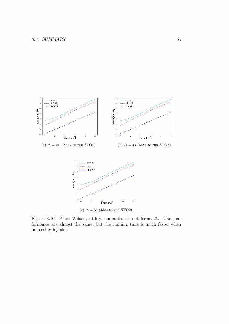
3.7. SUMMARY 55
(a) ∆ = 2s. (833s to run STO2). (b) ∆ = 4s (568s to run STO2).
(c) ∆ = 6s (438s to run STO2).
Figure 3.16: Place Wilson, utility comparison for different ∆. The per-formance are almost the same, but the running time is much faster whenincreasing big-slot.

56 CHAPTER 3. CHANNEL ALLOCATION ALGORITHMS
Figure 3.17: Jardin de Plantes,Toulouse with 4 BSs (Free and SFR)type 4G.
Figure 3.18: Utility Comparison:STO2, (PS)2S and PF-EXP.

Chapter 4
JOINT POWER CONTROLAND CHANNELALLOCATION
In this chapter, we consider the joint channel allocation and power controlproblem on the downlink, that is the transmit power of the BS can be var-ied subject to an average power constraint that does not exceed a certainavailable power budget to the BS. The objective is to design algorithms thatwork well for system with mobile users in order to improve proportional fair-ness. We propose two downlink scheduling algorithms that take advantageof partial information on future channel conditions, that is the mean of thechannel gains based on predicted future positions of the users, for improv-ing the sum utility. The scheduling model allows for both power control andchannel allocation. The objective of the scheduler is the long-term utility un-der an average power constraint. The two algorithms incorporate the channelpredictions in their decisions. The STO1 algorithm computes the decisionin each slot based on the means of future channel gains. Depending on thehorizon considered, this can require solving a large-dimensional problem ineach slot. The STO2 algorithm reduces the dimensionality by operating ontwo time-scales. On the slower scale it computes an estimation over a largerhorizon, and in the faster scale of a slot, it computes the decision based ona shorter horizon. Numerical experiments with both fixed number of usersas well as a dynamic number of users show that the two algorithms providegains in utility compared to agnostic ones.
57

58 CHAPTER 4. POWER CONTROL AND CHANNEL ALLOCATION
4.1 Introduction
Downlink scheduling and power control has been widely investigated for wire-less networks [39, 14, 29, 40]. In each time-slot, one or multiple base-stationshave to decide the users to serve and the transmit powers with the objectiveof maximizing the sum of the utilities of the users. Two different types of util-ities can be defined: (i) opportunistic [39, 14]; and (ii) long-term[29, 62]. Inthe opportunistic model, the utility function operates on the rate obtainedin a time-slot whereas in the long-term model, the utility operates on theaverage rate obtained over an horizon.
The focus of this chapter is on the long-term utility model. When trans-mit powers cannot be varied, the celebrated Proportional-Fair algorithm (see[37] and references therein) is known to work well when the utilities are log-arithmic functions of the total rate. This algorithm belongs to the class ofgradient-based algorithms that choose the user that maximizes the marginalutility or the gradient of the utility function. In [29] the gradient-based solu-tion was then extended to the setting in which joint power control and userscheduling is possible.
We revisit this problem in the context of vehicles which share theiritineraries with the decision maker. With the availability of SINR mapsin urban zones, the decisions can now be based also upon the future channelconditions of the users (or vehicles) [43]. The future channel conditions are,however, not known exactly as the they vary randomly in time. The SINRmaps are assumed to give the expected values of the channel gains on theroutes takes by the users. With this additional information on the future ex-pected channel gains, performance improvements can be expected comparedto the setting when this information is not available.
We consider a downlink scheduling and power control problem for onebase station with an average power constraint. The objective is the sumutility of the users, and the dependence of the utility function on the channelallocation and transmit power is similar to that in [29] with only one sub-channel and we do not have queues. In that respect, our model is a specialcase of that in [29]. However, the scheduling algorithms that we proposecan be extended to the multiple sub-channel case though for this chapter werestrict ourselves to the simpler case of one sub-channel. There are two dif-ference with the models studied previously. The first, and the main differenceis that the base station is also aware of the mean channel gains in the futureslots, and the second one is that we include an average power constraint overtime in the optimization problem.

4.1. INTRODUCTION 59
4.1.1 Contributions
We propose two heuristics for that use information on future channel con-ditions in order to improve the total utility. Both the heuristics were firstproposed in [51] in a setting without power control. The first one optimizesover future time-slots in every current slot whereas the second one reducesthe complexity by optimizing over the future time-slots only once in a certainnumber of slots. The performance of these heuristics will be evaluated onthree types of stochastic models for the channel gain processes. In the first,the channel gains are a stationary process with fixed mean channel gains(which can be different for different users) whereas in the second model, themean channel gains are themselves varying on a slower time-scale to that ofthe channel gains themselves. Finally in the third model, the mean chan-nel gains vary in every slot. For three models, these heuristics are shownto perform better than the other setting in which future information is notavailable.
4.1.2 Related work
Scheduling on the downlink but with fixed power examined in numerous pa-pers [11, 66, 13]. For a logarithmic utility function, the Proportional-Fair(PF) scheduler has been known to be optimal for stationary channel condi-tions [37] and its performance has been analyzed in both static and dynamicuser scenarios [10]. A restless bandit framework for network utility maxi-mization for channel states modeled as partially observable Markov chains isproposed in [40].
In [3], future rates are assumed to be known accurately over the optimiza-tion horizon and improvement in data rates and fairness is compared withalgorithms such as greedy (or max-rate) and equal share. Proportional-Fairalgorithms with partial information on future channel conditions have beenproposed in [7] (on short-time scales) and [43] (on longer-time scales). Thealgorithm in [43] is based on SINR maps that can be obtained from vehiclesor users that were present earlier. They proposed a PF-like index algorithmthat takes into account the future rate allocations using round-robin or a fewother heuristics. In [51], we proposed two heuristics that solve in each time-slot the utility maximization problem over a short-term horizon assumingthat the means of the future rates are known over this short horizon.
The joint optimization of channel allocation and transmit power controlhas been investigated for different multiplexing schemes such as like CDMA[62] and OFDM [29]. The proposed algorithms based their decisions onthe current channel conditions and previous decisions. In the context of

60 CHAPTER 4. POWER CONTROL AND CHANNEL ALLOCATION
high-speed trains, [77] solves the opportunistic utility maximization problemassuming all the future rates are known and with average power constraints.
4.2 Problem formulation
Consider a base station with K mobile users in its coverage range. In time-slot t, the base station transmits to user i with power pi(t). Assume thatuser i has a channel gain of γi(t) in slot t. These gains will be assumed tostochastic and independent between vehicles but not necessarily stationaryfor each user.
The received data rate for user i is computed according to the Shannonformula:
ri(t) = xi(t) log
(1 +
γi(t)pi(t)
xi(t)
), (4.1)
where xi(t) is the fraction of the channel assigned to user i is slot t. User igets a utility of Ui(z) when it obtains an average rate of z. In order to keepthe notation light, we will write ri(t) as a shorthand for ri(x, p, γ). Let S bethe appropriate dimensional simplex. We shall the use the notation
[xi(t)] ∈ S (4.2)
to mean that the vector [x1(t), . . . , xK(t)] ∈ S, where S is the K-dimensionalsimplex.
The utility function will be assumed to concave and differentiable. Awidely-used class of utility functions is that of the α-fair functions [45] thatare parameterized by α ≥ 0:
Ui(z) =
{z1−α
1−α , α 6= 1;
log(z), α = 1.
The special case of α = 1 is also known as the proportional-fair utility func-tion.
The objective of the base station is to choose the power and the channelallocation so as to maximize the total utility of these K users over a horizon

4.2. PROBLEM FORMULATION 61
of T time slots. That is, the base station solves the optimization problem:
maximizeK∑i=1
[Ui
(1
T
T∑t=1
ri(t)
)](OPT)
subject to [xi(t)] ∈ S,∀t; (4.3)
1
T
∑t
∑i
pi(t) ≤ P ; (4.4)∑i
pi(t) ≤ Pmax ∀t. (4.5)
Here P is the average transmit power budget available to the base station,and (4.4) is the average power constraint. This constraint also makes theproblem different from that in [29] where there was no constraint on theaverage power.
Remark 4.2.1 (Short-term fairness). A drawback of the utility function de-fined on the average rate is that if the scheduler knows that, for a particularuser, the channel gain may be very high some time in the future then it mightwait until this time to serve this user. This user may be starved of allocationsin the short-term and the solution may be unfair to this user on short-timescales. One way to resolve the short-term unfairness is to introduce addi-tional quality of service constraints such as requiring each user be scheduledat least once every given number of slots. This constraint was imposed in,for example, [43]. We can also include this constraint in the optimizationproblem. For simplicity, we do not impose it. We believe the results will besimilar as long as this constraint is not very restrictive.
Remark 4.2.2 (Fractional channel allocation). In (OPT) we have allowedfor fractional channel allocations. If the system imposes a binary constraint,that is only one user on one channel in any given slot, then these constraintscan be imposed in OPT as well as in the algorithms we propose. In theexperiments with a logarithmic utility function, we observed that allocationswere mostly binary. So, we expect the qualitative conclusions will be validwhether allocations are binary or not.
Remark 4.2.3 (Maximum power constraint). For conciseness, we shall notwrite the maximum power constraint explicitly in the optimization problemsthat we will define from now on. This constraint will be implicit and assumedto be applicable in all slots.
The current literature mostly solves (OPT) when the base station is awareof only the channel gains in the current slot1. For vehicles sharing their
1We shall use slot and time-slot interchangeably to mean the decision making instants.

62 CHAPTER 4. POWER CONTROL AND CHANNEL ALLOCATION
Coverage range of the BS
Channel gain
curve
Arrivals
Big slot
Figure 4.1: Mobility model.
itineraries, partial information on the future channel conditions could alsobe available to the decision maker in the current time-slot. We assume thatthis partial information is in the form of the mean of the channel gains in thefuture slots. One would expect to improve the value of the objective whenthis information is incorporated in the decision-making.
4.2.1 Channel gains
The heuristics will be evaluated on three different stochastic models for chan-nel gains: (i) the stationary model in which, for each vehicle i, γi(t) are inde-pendent and identically distributed across t with mean γi; (ii) non-stationaryand slowly varying model in which, for each vehicle i, the mean of the chan-nel gains varies on a slow time-scale. For example, for a time-slot of 2 ms,the means may vary every 100 slot or 200 ms; and (iii) a mobility model ona stretch of road, where cars can come and leave as shown in Fig. 4.1. Forthis model γi(t) are non-stationary, and also the mean of γi(t) changes everyslot.
Partial information on future channel conditions will be shown to behelpful for the second model and the third model. Nevertheless, the first (orthe stationary) model will still be useful to illustrate the benefits of beingable to vary the allocated power under an average power constraint.
4.3 Algorithms
In this section, we present the three algorithms that will be evaluated inthe numerical experiments. The first one is the standard gradient-basedscheduling which will be taken as the baseline. The other two are the oneswe propose in this chapter.
4.3. ALGORITHMS 63
4.3.1 Locally optimal algorithm
The locally optimal algorithm is a special case of the one in [29] for thescenario in which there is only one sub-channel and the power budget is Pin each slot. We remark that the algorithm can be handle the multiple sub-channel case but that in this chapter our focus is on the single sub-channelcase. When there is no average-power constraint as in [29], this algorithmchooses maximizes the objective function computed without the knowledgeof the future scheduling decisions. That is, in slot t, the scheduler solves
maximizeK∑i=1
[Ui
(1
t
t∑t=1
ri(t)
)](LA)
subject to [xi(t)] ∈ S,∀t; (4.6)∑i
pi(t) ≤ P ,∀t. (4.7)
Here, the past rate ri(s) for s = 1, 2, ..., t − 1 are known to the scheduler,so the decision variables are the channel allocations xi(t) and the transmitpowers pi(t) in slot t. The maximum power constraint is set to P in order tomake the comparison fair with algorithms which are subject to the averagepower constraint of P . For the logarithmic utility function, we shall call thisthe Proportion Fair (PF) solution.
4.3.2 Short-term Objective 1 (STO1)
We begin by defining a big-slot to be B consecutive time-slots. The firstheuristic we propose uses future mean channel gains to improve the objective.It includes in its decisions the future channel allocations and transmit powersbut only on the scale of big-slots. In each time-slot, the allocations arerecomputed for the current time-slot as well as the future big-slots. Theintuition behind this is to maximize in each slot the long-term objectivebased on the best information available. We explain its workings in thecontext of the non-stationary slowly varying channel model and the mobilitymodel.
For the slowly varying model, B will be the number of time-slots duringwhich mean channel gain remains constant whereas in for the mobility modelB can be set by the system designer depending on how fast the mean channelgains vary. Let T = T/B be the number of big-slots in the horizon, and letτt ∈ {1, . . . , T} be the big-slot to which time-slot t belongs to, and let θt bethe number of slots remaining in big-slot τt not including t, that is
θt = (τt + 1)B − t.

64 CHAPTER 4. POWER CONTROL AND CHANNEL ALLOCATION
We shall use the notation x for a quantity that is computed over a big-slot.For example pi(τ) will denote the power used in all the slots inside big-slotτ . Similarly,
ri(τ) = Bxi(τ) log
(1 +
γi(τ)pi(τ)
xi(τ)
)(4.8)
is the total rate obtained by vehicle i in big-slot τ when it is served xi(τ)fraction of time at a transmit power of pi(τ). Note that here the rate iscomputed assuming that the channel gain is its mean value in big-slot τ .With slight abuse of notation,
ri(τt) = θtxi(τt) log
(1 +
γi(τt)pi(τt)
xi(τt)
), (4.9)
shall denote the total rate in the remaining slots in current big-slot τt. Also,define
Pt = T P −K∑i=1
t−1∑s=1
pi(s)
to be the total remaining power available to the scheduler in slot t.In each slot, STO1 maximizes
K∑i=1
Ui
1
T
t−1∑s=1
ri(s) + ri(t) +T∑
τ=τt
ri(τ)
(STO1)
subject to
[xi(t)] ∈ S; [xi(τ)] ∈ S, τ = τt, . . . , T ; (4.10)
K∑i=1
pi(t) + θtpi(τt) +T∑
τ=τt+1
Bpi(τ)
≤ Pt. (4.11)
The variables in this problem are [pi(t)] and [pi(τ)], τ = τt . . . T , and thecorresponding channel allocations. In (4.11), the LHS is the total transmitpower starting from the current slot which has to be less than the remainingpower Pt.
For the mobile model, instead of solving (STO1-Opt) over the wholehorizon T , we solve it on a shorter horizon, which is equal to the maximumstaying time of the users currently inside the system. This shorter timehorizon can vary from one slot to another, and it explains the words ’short-term objective’ in the name of the algorithm. The advantages of this is toreduce the computation time which can be helpful when the algorithm hasto be executed every 1ms.

4.3. ALGORITHMS 65
4.3.3 Short-term Objective 2 (STO2)
The STO1 algorithm recomputes in each time slot the optimal solution of thefuture big-slots. In STO2, we recompute the solution of the future big-slotsonly at the beginning of each big-slot. Inside a big-slot, we compute only thesolution for the current slot assuming the solution for the future big-slots tobe the same as that computed at the the start of the current big-slot. Thatis if t ≡ 1 (mod B), STO2 first maximizes
K∑i=1
Ui
1
T
t−1∑s=1
ri(s) +T∑
τ=τt
ri(τ)
(STO2-Big)
subject to
[xi(τ)] ∈ S, τ = τt, . . . , T (4.12)
BK∑i=1
T∑τ=τt
pi(τ) ≤ Pt. (4.13)
The variables in this problem are [xi(τ)] and [pi(τ)], τ = τt . . . T .Next, in each slot t, we compute the optimal allocation and transmit
power assuming that the allocations and transmit powers in the future big-slots are those computed from solving (STO2-Big). In slot t, STO2 maxi-mizes
K∑i=1
Ui
1
T
t−1∑s=1
ri(s) + ri(t) +T∑
τ=τt
ri(τ)
(STO2-Small)
subject to
[xi(t)] ∈ S, [xi(τt)] ∈ S; (4.14)
K∑i=1
(pi(t) + θtpi(τt)) ≤ Pt −K∑i=1
T∑τ=τt+1
Bpi(τ). (4.15)
The variables in this problem are [xi(t)], [pi(t)], [xi(τt)] and [pi(τt)]. Ascan be seen, in a slot the dimension of the problem is no bigger than the onefor STO1. As in STO1, for the mobile model, STO2 solves (STO2-Big) and(STO2-Small) over a shorter horizion which is the maximum staying timeof the users currently in the coverage range. The pseudo code for STO2 isshown in Algorithm 4.
In terms of computational effort, compared to STO1, STO2 solves a lowerdimensional problem in each slot except at the starting of every big-slot wherethe dimension is same as for STO1. Thus, one can except it to be faster butfurther from the optimal solution.

66 CHAPTER 4. POWER CONTROL AND CHANNEL ALLOCATION
ALGORITHM 4: The STO2 algorithm
t← 1while t ≤ T do
if t ≡ 0 mod B thenSolve (STO2-Big) and obtain x(τ) and p(τ).Solve (STO2-Small)
elseSolve (STO2-Small)
end
end
4.4 Numerical experiments
The numerical experiments were run in Python, and all optimization prob-lems were solved using the python package CVXPY [20] and the solverMOSEK. The results will be presented according to the channel-gain models.For the stationary and slowly varying channel models, we assume that thenumber of users is fixed. The third model will be evaluated in a dynamicsetting in which users will arrive and leave the network.
In all the experiments, P is set to 15 and Pmax is set to 30. Whenever weshow any performance measure of the optimal solution, it will be assumedto mean that the optimal is computed assuming all the future channel gainsare known exactly.
4.4.1 Stationary channel
For the first experiment, we take K = 4, that is four users, and a logarithmicutility function for every user. The vector of means [γi] = [6.76, 5.45, 4.35, 1.31].The channel gain in slot t for user i is generated as follows:
γi(t) = γiAi(t; η) (4.16)
Here Ai(t; η) is a sequence of i.i.d. uniform random variable in the range[1− η, 1 + η]. We shall refer to η as the noise level. It is assumed that Ai(t)and Aj(t) are assumed to be independent for i 6= j. Varying η from 0 to 1changes the variance of Ai(t) from low to high. For η = 0, the channel gainsbecome deterministic and known to the decision maker.
Remark 4.4.1. The method for generating γi(t) need not be necessarily mul-tiplicative as in (4.16). Our heuristics can be used as long as the means ofthe future channel gains are known. In this chapter, we limit the numericalevaluation to the form in (4.16).

4.4. NUMERICAL EXPERIMENTS 67
0.0 0.2 0.4 0.6 0.8 1.0Noise level ( )
0.7
0.6
0.5
0.4
0.3
0.2
Tota
l Util
ity
PFSTO2STO1STO1FPOPT
Figure 4.2: Total utility as a function of noise level. Channel is stationary.Log utility function.
Figure 4.2 shows the total utility as a function of the noise level η. Thetime horizon T was taken to be 500 with 5 big-slots, that is, one big-slot hasB = 100. If the scheduling slot is 1 ms as in 4G [19], then the schedulinghorizon is of 500 ms. Five sample paths for channel gains were generated,and the plot shows the average of these 5 samples. The label PF is for thelocal optimization algorithm. The suffix FP attached to STO1 means thatSTO1 was run wilth a fixed power budget of P in each slot.
As expected, allowing for an average transmit power constraint and usingfuture information (even if it is just the mean channel gains) improves theutility. When η = 0, all the algorithms are equivalent and give the sameutility since the channel gain is the same is every time slot and is known.Further, performance improvement is more when the noise variance is higherwhich is again to be expected.
4.4.2 Slowly varying channel
Next, we conduct experiments with the slowly varying channel model. It isassumed that the channel means are constant during B = 100 slots. Theoptimization horizon is T = 2000, that is there are 20 big-slots in each run.

68 CHAPTER 4. POWER CONTROL AND CHANNEL ALLOCATION
The mean channel gains were first determined for each big-slot. Within abig-slot, the channel gains were then generated using the same method as forthe stationary case and given in (4.16). The number of users was again setto 4.
In the first experiment, the mean channel gains are relatively homoge-neous with an empirical average of the mean channel gains being [5.98, 5.55,4.69, 5.30]. Figure 4.3a, plots the total utility as a function of the noise levelwhile Fig. 4.3b shows the total transmit power in a slot as a function oftime-slot. The data in the latter plot was obtained on a separate run withB = 50, η = 1, and only STO2 and OPT are shown so as to have a morereadable figure.
We observe that all algorithms except PF are close to optimal almostthroughout. Since the total transmit power in a slot is not far from P ,STO1FP is almost as good as STO1. However, in this scenario prediction isstill useful as PF is away from OPT even for η = 0, that is when there is nonoise.
The mean channel gains in the second experiment are widely varying withthe empirical average of the mean channel gains being [2.63, 10.3, 3.76, 0.009].One user is in a very bad channel state, whereas another one has much bettermean channel gains than the others. The plots for the total utility and totaltransmit power in a slot are shown in Fig. 4.4. Again, the total power wascomputed from a separate run.
This time we observe that both power control and channel predictionresult in improvements. Due to one user being much worse than the others,the optimal transmit power varies much more than in the previous experimentand hits the maximum constraint quite often. Since the fixed-power versionis inflexible in this respect, it performs worse for all noise levels.
4.4.3 Mobility Model
Consider a stretch of road of length 1 km covered by one base station, in whichvehicles enter from the left and leave on the right (Fig. 4.1). To simplify forillustration, we assume they move with same velocity v = 25 m/s, but thealgorithms presented in Sec. 4.3 do not depend on this assumption. So theystay in the coverage range of the base station in 40 seconds. New vehiclescan enter the network only at the start of the big-slots. The length of abig-slot is set to 1 sec. The probability of a new arrival in a big-slot is setto p = 0.3. For each value of noise level (η) we simulate this network for 800seconds. In this model, the channel gain of mobile user is non-stationary andvaries every time slot (1 ms), STO1 and STO2 solves over an horizon of 40seconds which is the staying time of users in the network. These two aspects

4.4. NUMERICAL EXPERIMENTS 69
0.0 0.2 0.4 0.6 0.8 1.0Noise level ( )
0.55
0.60
0.65
0.70
0.75
0.80
0.85
Tota
l Util
ity
PFSTO2STO1STO1FPOPT
(a) Total utility vs. noise level
0 100 200 300 400 500Time-slot
14
15
16
17
18
Tota
l tra
nsm
it po
wer p
er sl
ot
STO2OPT
(b) Total allocated power per slot vs. time-slot
Figure 4.3: Slowly varying channel. Log utility function. Experiment 1.η = 1.

70 CHAPTER 4. POWER CONTROL AND CHANNEL ALLOCATION
0.0 0.2 0.4 0.6 0.8 1.0Noise level ( )
2.6
2.5
2.4
2.3
2.2
2.1
2.0
1.9
Tota
l Util
ity
PFSTO2STO1STO1FPOPT
(a) Total utility vs. noise level
0 100 200 300 400 500Time-slot
5
10
15
20
25
30
Tota
l tra
nsm
it po
wer p
er sl
ot
STO2OPT
(b) Total allocated power per slot vs. time-slot
Figure 4.4: Slowly varying channel. Log utility function. Experiment 2.η = 1.

4.5. SUMMARY 71
Figure 4.5: Channel gain for two cases: with noise (η = 0.2) and withoutnoise.
make this model different from the two first models. Since the dimension of(OPT) is very large in this case, we do not compute the optimal solutionin the experiments. Also, since STO1 solves a high dimensional problem inevery slot compared to STO2, it is much slower when the horizon is large.So, we show only the performance of STO2 and PF.
Fig. 4.5 illustrates the channel gain curve in the noise and no noise cases.Here, the rate is a function of users’ position which is in fact a function of thedistance to the base station. Let us take the left margin of the road be 0, andthe right margin be 1000, then for position x ∈ [0, 1000] inside the coveragerange, the channel gain is equal to f(x) = β(1 + κ exp(|500 − x|/σ). Here,β, κ, σ are adjustable parameters; in our experiment β = 0.01, κ = 40, σ =200.
Fig. 4.6 illustrates the numerical results for the above mobile system.The total allocated power is shown only for a small interval of time. Again,we observe that channel prediction leads to a better total utility. Further, byobservation, STO2 allocates more power when there are many users (thanusual) close to the peak where channel gains are good with high probability.
4.5 Summary
We proposed two heuristics for joint power control and channel allocationthat exploit partial information future channel conditions to improve theutility. Even little information such as mean channel gains is sufficient to

72 CHAPTER 4. POWER CONTROL AND CHANNEL ALLOCATION
0.0 0.2 0.4 0.6 0.8 1.0
Noise level
2.5
2.4
2.3
2.2
2.1
2.0
1.9
1.8
Tota
l Util
ity
STO1STO1FPSTO2PF
(a) Total utility vs. noise level
250 300 350 400 450 500
Time (in seconds)
5
10
15
20
25
Tota
l tra
nsm
it po
wer p
er sl
ot
STO1STO2PF
(b) Total allocated power vs. time (in second). η = 0.2.
Figure 4.6: Mobility model. Log utility function.

4.5. SUMMARY 73
observe improvement compared to when no information is used.The heuristics are well performed but they are quite heavy since they
have to solve an optimization problem frequently (every time-slot for STO1and every big slot for STO2). In chapter 5 we shall use machine learningbased method to learn STO1 to produce an approximate algorithm with lesscomputing time.

74 CHAPTER 4. POWER CONTROL AND CHANNEL ALLOCATION

Chapter 5
LEARNING THE CHANNELALLOCATION ALGORITHM
5.1 Abstract
In Chapter 3 and Chapter 4, we have introduced two heuristic schedulingalgorithms that can be applied to general networks. However, in those algo-rithms, an optimization problem needs to be solved frequently which requiresa costly computation and thus may impair real-time processing for large net-works. In this chapter, we propose to use Deep Feedforward Neural Networks(DFNN) for learning the relation between inputs and outputs of one of thosealgorithms. It yields an approximate solution with much less computationtime.
5.2 Introduction
Due to the limited availability of resources and to the heterogeneity of userrequirements, a proper scheduler plays an important role for an effectivesharing of network resources between users and for improving the quality ofservice. Solving the scheduling problem often amounts to solving a large-scaleoptimization problem [62], [43]. As has been shown numerically in Chapter3 and Chapter 4, we can improve the user allocation by taking into accountall the available information (that is, past and current information as wellas a partial future information) and then solving an optimization problembased on this information. This is what is done by the STO1 algorithm.However, solving large-scale optimization problems so frequently (i.e. everyfew milliseconds) poses a new challenge: real time processing.
In this chapter, we propose a machine learning-based approach to obtain
75

76 CHAPTER 5. LEARNING ALGORITHM
an approximate solution to the scheduling problem with much less compu-tation time as compared to the STO1 algorithm. The key idea is to use afunction of DFNN form to express approximately the relation between theinputs and the outputs of STO1.
5.2.1 Related works
The theory of approximation for DFNN has been studied in many papers.Motivated by Komogorov’s superposition theorem [35] in 1957, many approx-imation results have proven the approximation capabilities of feed-forwardneural networks for the class of continuous functions such as [18],[28],[47].In his theorem, Komogorov proved that any continuous function can be rep-resented as a superposition of continuous functions of one variable. In [18](1989), Cybenko proved that any multivariate continuous function with sup-port in a hypercube can be uniformly approximated by a linear finite combi-nations of compositions of a sigmoidal functions and a set of affine functions.This representation is in fact a feed-forward neural networks with sigmoidalactivation function. Independently with the work of Cybenko, Hornik [28](1989) also proved a similar result. Two years later, Hornik [27] showedthat multi-layer feed-forward neural networks with arbitrary bounded andnon-constant activation function can approximate arbitrary well real-valuedcontinuous functions on compact subsets of Rn as long as sufficiently manyhidden layers are available. The word ”deep” in ”deep learning” thus simplymeans many layers.
Learning an algorithm to produce an approximate algorithm in order toreduce computation time has been proposed in several recent research papers[24], [63]. In [24], the authors consider a Sparse Coding problem which is usedfor extracting features from raw data. The problem is that Sparse Coding isoften too slow for real-time processing in several applications such as patternrecognition. The authors propose a method using a non linear, feed-forwardfunction to learn Sparse Coding to produce an approximate algorithm with10 times less computation.
Learning an algorithm for wireless resource management by DFNN hasbeen proposed in [63]. In that work, the authors used DFNN to learn analgorithm for the interference channel power control problem. They obtainan almost real time algorithm, since passing the input through a DFNN toget the output only requires a small number of simple operations as com-pared to an iterative optimization algorithm. They show that, by choosingan appropriate initialization, the initial power control algorithm performs acontinuous mapping which can be efficiently learnt.
In this chapter, we use DFNNs for learning a channel allocation algorithm

5.2. INTRODUCTION 77
maximizing the proportional fairness between vehicular users. The proposedmethod is however potentially applicable to other convex optimization prob-lems.
5.2.2 Contributions
We first propose a machine learning based method for learning the STO1algorithm introduced in Chapter 3 and Chapter 4. We compare differentDFNN architectures and different loss functions to find the most appropriateones for our problem.
As discussed in Section 5.2.1, any continuous function can be approxi-mated arbitrary well by a DFNN. However, discontinuous functions are muchmore difficult to learn. Unfortunately, as we show with a simple example, theinput-output mapping realized by the STO1 algorithm is discontinuous. Thismakes the model slower to learn due to oscillations at discontinuity points.
We then characterize these discontinuity points of STO1 by explicitlyindicating the set where they reside. In a small dimension, we use thischaracterization to propose a simple user ordering scheme and a method forchoosing the output when the solution is not unique which make the STO1mapping continuous, and thus hopefully easier to learn. Unfortunately, inlarger dimensions, finding an appropriate order requires to solve the originaloptimization problem which we are trying to avoid solving. We thus proposeseveral heuristic ordering schemes. Although they do no necessarily resultin a continuous function, numerical results show that these heuristic ordersallow to reduce the learning time. However, these heuristic orders do notalways increase accuracy.
Finally, we propose another approach which amounts to learning the dualvalues, which are proven mathematically to be continuous. Numerical resultsin section 5.6.5 show that learning dual values is faster and has better per-formance in comparison with learning the primal values.
5.2.3 Organization
In Section 5.3, we recall the resource allocation problem introduced in Chap-ter 3 in the case of a single Base Station (BS). We also remind the readerof the STO1 algorithm and state the learning problem we address in thischapter. In Section 5.4, we formally define the input-output relationship forthe DFNN model. We discuss about the continuity of this input-output map-ping in Section 5.5 and then propose to learn dual values as well as severaluser ordering schemes for reducing the discontinuity of the original mapping.Numerical results are presented in Section 5.6. We compare the computing
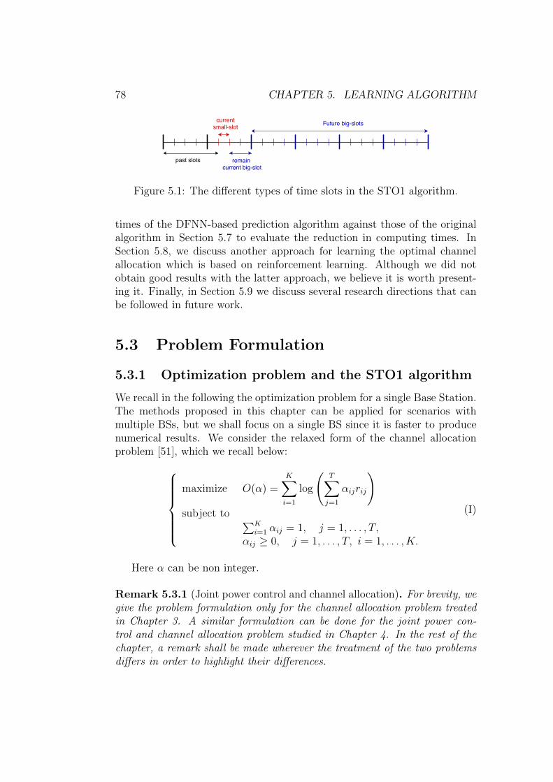
78 CHAPTER 5. LEARNING ALGORITHM
past slots
currentsmall-slot
remain current big-slot
Future big-slots
Figure 5.1: The different types of time slots in the STO1 algorithm.
times of the DFNN-based prediction algorithm against those of the originalalgorithm in Section 5.7 to evaluate the reduction in computing times. InSection 5.8, we discuss another approach for learning the optimal channelallocation which is based on reinforcement learning. Although we did notobtain good results with the latter approach, we believe it is worth present-ing it. Finally, in Section 5.9 we discuss several research directions that canbe followed in future work.
5.3 Problem Formulation
5.3.1 Optimization problem and the STO1 algorithm
We recall in the following the optimization problem for a single Base Station.The methods proposed in this chapter can be applied for scenarios withmultiple BSs, but we shall focus on a single BS since it is faster to producenumerical results. We consider the relaxed form of the channel allocationproblem [51], which we recall below:
maximize O(α) =K∑i=1
log
(T∑j=1
αijrij
)subject to ∑K
i=1 αij = 1, j = 1, . . . , T,αij ≥ 0, j = 1, . . . , T, i = 1, . . . , K.
(I)
Here α can be non integer.
Remark 5.3.1 (Joint power control and channel allocation). For brevity, wegive the problem formulation only for the channel allocation problem treatedin Chapter 3. A similar formulation can be done for the joint power con-trol and channel allocation problem studied in Chapter 4. In the rest of thechapter, a remark shall be made wherever the treatment of the two problemsdiffers in order to highlight their differences.
5.3. PROBLEM FORMULATION 79
Let ∆ be the size of the big-slot in absolute time units and let m = ∆/δbe the number of small slots in a big-slot (see Figure 5.1). Denote by rij themean rate in slot j for user i (we shall assume it is a function of distancefrom the user to the BS). At each small-slot t, with a slight abuse of notation,
we shall denote by ρi,0 =∑(m−(t mod m))+t
j=t+1 rij the total rate for user i in theremaining channel allocation slots of the current big-slot τ = 0, where tmod m denotes the remainder when dividing t by m. We also define αi,0 asthe corresponding allocation for the current big-slot τ = 0.
Denote by ρiτ =∑τm+A
j=(τ−1)m+A+1 rij where A =(⌊
tm
⌋+ 1)m, is the total
average data rate that user i will get in the future big-slot τ (τ = 1, 2, ..., J−1), where big slot τ starts after the current big-slot, and J is the short timehorizon in term of big slots over which we can estimate the mean future rate.We also define αiτ as be the corresponding allocation for user i in future bigslot τ . These allocations αiτ can be interpreted as the fraction of small slotsthat user i will be allocated in the big-slot τ .
Note that this definition is slightly different from definition in chapter 3.The differences are as follows: in chapter 3, there is no current big slot andthe future big-slot starts just after the current small slots, but it does notchange much. The above definition of two time slot types corresponds in factto the ones introduced in Chapter 4.
Denote by ai(t) =∑t
j=1 αijrij the total throughput allocated to user i upto time slot t, and let K(t) be the number of users inside the coverage rangeof the BS at time t.
The algorithm STO1 contains two steps which are as follows:
• Step 1– solve the following optimization problem over a short-termhorizon of J big-slots:
maximize
K(t)∑i=1
log
(ai(t− 1) + αitrit +
J∑τ=1
αiτ ρiτ
)subject to ∑K(t)
i=1 αit = 1,∑K(t)i=1 αiτ = 1, τ = 0, . . . , J − 1,
αit, αiτ ∈ [0, 1], , τ = 0, . . . , J − 1, i = 1, . . . , K(t).(STO1-Opt)
The decision variables in Problem (STO1-Opt) are the channel alloca-tions in the current small slot, αit, and the channel allocations in thecurrent and future big-slots, αiτ . Since the future allocations are onlycomputed on the time-scale of big-slots, there is a reduction by factorm in the number of variables in (STO1-Opt).

80 CHAPTER 5. LEARNING ALGORITHM
Figure 5.2: The Carmes borough in Toulouse, with one BS (Free Mobile typeLTE1800). The actual size is 200m× 400m.
• Step 2 – allocate the channel to the users with the fraction αit ofcomputed allocation in the current small-slot t.
Here in step 2, we consider the relaxed solution which is different fromSTO1 in Chapter 3 (which rounds the relaxed solution to obtain an integersolution) since we want to use the properties of convex optimization prob-lems to investigate the continuity of the solution. After learning the optimal(fractional) allocation, we will come back to an integer solution by allocatingthe channel to the user with the largest fraction αit. Actually, we observedthat the solutions of (I) and (STO1-Opt) are integer with high probability.Figure 5.3 shows STO1 with integer version and STO1 with relaxed versionfor a scenario generated with SUMO using the map shown in Figure 5.2with 244 users in around 61.7 minutes (the other parameters are identical tothose used in Section 5.6.1). We can notice that the behaviors are not muchdifferent.
Remark 5.3.2. (STO1-Opt) is solved thanks to the python package CVXPY[20] and the solver MOSEK. In Chapter 3, we solve this optimization problemusing a projected gradient algorithm, since this method allows to approximatesolution of a convex optimization problem by iterations when the feasible set isof simplex form (i.e, a simplex or a Cartesian product of simplex), no matterhow complex the objective function is as long as it is smooth and convex. Buthere we employ CVXPY [20] since it can be used to generalize this idea toother convex optimization problems, with more complex constraints such aspower control constraints or others QoS constraints (e.g. delay constraints).

5.3. PROBLEM FORMULATION 81
0.0 0.2 0.4 0.6 0.8 1.0noise level
7.1
7.0
6.9
6.8
6.7
6.6av
erag
e to
tal u
tility
STO1 integerSTO1 relaxed(PF)2SPF
Figure 5.3: Comparison of integer and relaxed versions of STO1.
5.3.2 Learning STO1 with DFNN
As presented in Chapter 3 and Chapter 4, STO1 and STO2 are better thanthe other existing algorithms. However they have to solve an optimizationproblem with a large number of variables and constraints frequently (everysmall slot for STO1 or every big slot for STO2), so even if their performance isgood, their computations are heavy. When the system is large and requiresmany more QoS contraints, they may not be able to run in real time. Inaddition, even when they are able to run in real time, it is good to reduce thecomputation time without reducing too much the quality of the allocation.
Therefore in this chapter, we want to learn the STO1 algorithm usingDeep Feedforward Neural Networks to obtain a new algorithm that behaveslike STO1 but with a significantly reduced computation time. In other words,we want to learn the input-output relationship of STO1, by approximatingthe input-output mapping of STO1 with a DFNN. Here we focus only onSTO1, but a similar approach is expected to work for STO2. After gettingthe approximation function (that is, the DFNN), the output can be computedby feeding the DFNN with the input value, instead of solving an optimizationproblem. This simpler method is expected to work faster than the originalalgorithm.
Obviously, the same idea could be used for other problems in order toobtain an approximate method which performs almost as well as the originalalgorithm but requires much less computing time. In short, the approach isas follows:
1. Design a well-performing algorithm based on the best available infor-

82 CHAPTER 5. LEARNING ALGORITHM
Output:Allocation
Input: state of the system
a
bc
Hidden layers
Figure 5.4: An example of Deep Feed-forward Neural Network.
mation;
2. Learn it by an approximate algorithm which behaves closely to theoriginal one and has less computation.
The background on supervised learning with DFNN was presented inSection 2.5.2. The basic idea can be summarized as follows. The STO1algorithm can be seen as a function F that maps an input X ∈ X (a probleminstance) to an output Y ∈ Y (a channel allocation), where X and Y denotethe input and output spaces of STO1, respectively. Unfortunately, STO1 istoo complicated to get the exact formula of F . Therefore here we want toapproximate it by another function F : X → Y which is in the form of aDFNN (an example of DFNN is illustrated in Figure. 5.4).
A DFNN is composed of many linear functions (sum of matrix multipli-cations and bias vectors) and non-linear functions (relu, sigmoid, softmax,etc [76]), and inside linear functions there are many parameters. So findinga good DFNN function means finding a good architecture, that is: the waythe linear and non-linear functions are combined, the linear and non-linearfunctions in each layer, the size (number of units in each hidden layer) andthen their parameters. Finding a good architecture is in general not an easytask [64]. In this chapter, we shall empirically compare some architecturesthrough experiments presented in Section 5.6.2. After fixing the architecture,we have to find appropriate parameters by minimizing the empirical risk asdescribed in Section 2.5.2.

5.4. SYSTEM SETUP FOR LEARNING 83
5.4 System Setup for learning
Recall that, in STO1, we have two types of time scales: one is the big slot ∆and the other one is the small slot δ. In STO1, we solve problem (STO1-Opt)with variables of size (1+J)∗K every small slot, where J is the time horizonin terms of big slots and K is the number of users in the system. The sizeof the allocation vector for each user is equal to 1 + J since it contains theallocation for the current small slot, αit, and the average allocation αiτ for thesubsequent J big slots (including the current big slot). The input of STO1 isa data rate vector of size (1+J)∗K and the total allocated throughput for theK users. The output of STO1 is the current allocation vector (αit)i=1,...,K
which is of size K, since we shall only use current allocation for makingdecision.
As it is defined at the moment, STO1 is not well suited to be modelledas a learning problem for the two reasons stated below.
Firstly, since K can vary over time, the dimension of the input vectorwill also vary. To circumvent this problem and to properly define STO1 asa function, we have to fix the size of the state. To do that, we extend thereal state of the system by adding some pseudo users. Let us assume thatthere are at most KM users inside the system. We will then add KM − Kpseudo users, where K is the number of real users in the system at time t.We will actually learn an extended version of STO1 which is STO1 whenwe restrict it to K users. There are many ways to extend STO1, but herewe try to define an extended version that preserves as much as possible thecontinuity of STO1. When we mention ”learning STO1”, it means ”learningthe extended function” of STO1.
Secondly, the output of STO1 as defined above is the solution of an opti-mization problem. So in fact STO1 is a set-valued mapping since the solutionneed not be unique. But by using the CVXPY package to solve the convexoptimization problem (STO1-Opt), we agree with the way it determines oneof the solutions. This makes STO1 becomes a function (instead of set-valuedmapping). However, the way the solution is chosen when it is not unique canmake the function become continuous or discontinuous. In [63], the authorsshow that a mapping can be made continuous by choosing an appropriateinitial point for the algorithm. We shall discuss the continuity of the STO1function and how to choose the solution when it is not unique in order toobtain a continuous mapping in a small dimension in Section 5.5.
Remark 5.4.1 (Joint power control and channel allocation). For the jointpower control and channel allocation problem, the state needs to be augmentedby the remaining total power. The output of the DFNN will now give the
84 CHAPTER 5. LEARNING ALGORITHM
transmit power to each user as well as the fraction of the channel it getsallocated.
5.4.1 State
We define a state as a matrix of size (2+J)×KM , where KM is the maximumnumber of users in the system. There are thus 2 + J rows, and each row hasKM elements. The interpretation is as follows:
• The first row gives the current rates of the K users. We fill in theK positions on the left hand side with these current rates, and theremaining KM −K positions are filled with −1.
• The next J rows (from 2, .., J + 1) give the average rates of the usersin the next J big slots. For pseudo users (the KM −K columns on theright hand side), we use the value (−1) · (∆/δ − (t mod ∆/δ)) for thecurrent big slot and the value (−1) ·∆/δ for the other big slots.
• The last row gives the total allocated throughput of the K users. Forpseudo users, we use a large enough value which is significantly greaterthan the total allocated throughput of real users.
By observing how STO1 works, we remark, as expected, that STO1 givespriority to users with a low allocated throughput and a high current rate.Therefore, the way we define the state (that is, by using by negative numbersfor the current and future rates of pseudo users, and extremely large valuesfor their allocated throughput) is intended to help the model ignore quicklythe pseudo users.
Remark 5.4.2. Remark that the real K users in the system at present time.Therefore, the K places of the real users in the first row which give the currentrates of those users have to be strictly positive. The future rates (from thesecond row to the (J + 1)-th row) can be zero.
5.4.2 Target
We remind the reader that we want to learn only the current allocation, notthe future allocation. Therefore, the target will be a vector of size KM , wherethe first K positions represent the fractional allocation αit of the K users ascomputed by STO1, and the last positions are filled with zero. Since inthe optimization problem, the sum of allocation should be equal to 1, whenthere is no user in the system (all positions correspond to pseudo users), theallocation vector will be set to (1/KM , ..., 1/KM) by convention.

5.5. DISCUSSION ABOUT THE CONTINUITY OF THE STO1 FUNCTION85
Current Rate
Cumulative
F (STO1)Future Rate in next
J big-slotsAllocation
Figure 5.5: Input and output of the DFNN model.
0-1current rate
Figure 5.6: Two connected components of Ei,1∀i.
Figure 5.5 illustrates the input and output of the DFNN model as de-scribed above.
Remark 5.4.3. From now on, we shall denote by F the input-output map-ping realized by STO1 when its output is restricted to the current allocationvector (αit)i=1,...,K . One could of course learn the full allocation matrix (thatis, including future allocations αiτ over the big slots), in which case the outputwould be of size (J + 1) ∗KM instead of size KM . By doing that, the outputprovides more information than the way it was defined above. However, asSTO1 is not a continuous function as we shall shortly discuss, the definitionproposed here eases the characterization of discontinuity points.
5.5 Discussion about the continuity of the
STO1 function
As defined above, F is a mapping from∏i=KM ,j=J+2
i=1,j=1 Ei,j to SKM , where SKMis the simplex of size KM and
• For j = 1 and i = 1, . . . , KM , Ei,1 = (0,+∞] ∪ {−1},
• For j = 2, . . . , J+1 and i = 1, . . . , KM , Ei,j = [0,+∞]∪{−1,−2, ...,−∆/δ},
• For j = J + 2 and i = 1, . . . , KM , Ei,J+2 = [0,+∞].
We can see that the pseudo users and real users lie in different connectedcomponents (see Figure 5.6), from which it follows that the continuity of itsextension depends only on STO1. We shall thus concentrate on the continuity

86 CHAPTER 5. DISCUSSION ABOUT CONTINUITY OF STO1
of the STO1 function on the connected component corresponding to the Kreal users. Unfortunately, STO1 itself is not a continuous function. Let ustake a simple example illustrating the discontinuity. Assume that K = 2,J = 1, ∆ = δ and consider the following sequence of states:
Rn =
r +(
1n
)· (−1)n r −
(1n
)· (−1)n
r −(
1n
)· (−1)n r +
(1n
)· (−1)n
0 0
.
Then it is easy to show that Rn → R, where
R =
r rr r0 0
.
However
F (Rn) =
{[1, 0] if n = 2k,
[0, 1] if n = 2k + 1.
This simple example shows that the STO1 function is not continuous.The discontinuities make the learning problem much more difficult since neardiscontinuity points, the DFNN model does not know which direction of theoutput its parameters should follow. For example, as illustrated in the above2-dimension example, near R, the target (output) oscillates between [0, 1]and [1, 0]. Since a DFNN-based function is a composition of many continuousfunctions, it is also a continuous function. Trying to fit every target near Rinto the DFNN model can make its parameters conflict and result in a slowerconvergence. Therefore in the remainder this section we shall characterizethe discontinuity points of the STO1 function and discuss how to derive acontinuous function from STO1.
Above we showed one discontinuity point (R) when K = 2, J = 1. Now,our objective is to characterize the set containing all discontinuity points.Before doing that, let us analyze the property of an optimal solution resultingfrom the KKT conditions (which are necessary and sufficient conditions inour case as presented in section 2.5.1). To simplify the notation, let us assumethat a big slot is equal to a small slot, that is, ∆ = δ (the proof is howeverstill valid if a big slot is equal to multiple small slots). With ∆ = δ, we canwrite (STO1-Opt) as follows:
maximize
K(t)∑i=1
log
(t+J∑j=t
αijrij + ci
)∑K(t)
i=1 αij = 1, j = t, t+ 1, ..., t+ J,αij ∈ [0, 1], j = t, t+ 1, ..., t+ J, i = 1, . . . , K(t).
(IR)

87
Let us denote by rij the rate of user i at time j, and let ci be the totalthroughput allocated to user i up to present time. Consider the state Rdefined by
R =
r1t r2t · · · rKM t· · · · · · · · · · · ·r1,t+J r2,t+J · · · rKM ,t+Jc1 c2 · · · cKM
,
in which the ith column provides all the information available for user i. Wedenote the above optimization problem by (IR) to emphasize that it dependson R.
The Lagrange function of this convex optimization problem is L = O(α)+∑j λj(1−
∑i αij) +
∑i,j ρi,jαij where O(α) =
∑K(t)i=1 log
(∑t+Jj=t αijrij + ci
).
The KKT conditions for problem (IR) are as follows:
1, Primal feasibility:
∑i α∗ij = 1 ∀j, and α∗ij ≥ 0 ∀i, j,
2, Dual feasibility: ρ∗ij ≥ 0 ∀i, j,3, Complementary slackness: α∗ijρ
∗ij = 0 ∀i, j,
4, Lagrange stationary:ri,j
ci+∑k α∗ikrik
= λ∗j − ρ∗ij ∀i, j.
(KKT)
The last condition is implied by ∇αL(α∗) = 0.From (KKT), it follows that if ρ∗ij > 0, then α∗ij = 0 and
ri,jci+
∑k α∗ikrik
=
λ∗j−ρ∗ij < λ∗j . It implies that α∗ij is positive only when ρ∗ij = 0 and in this casethe ratio
ri,jci+
∑k α∗ikrik
= λ∗j represents the maximum ratio one user i can get
in slot j. Since∑
i α∗ij = 1, there exists at least one user who gets a strictly
positive allocation in time slot j, i.e, there exists at least one user i for whichρ∗ij = 0. The output that we consider is only the current allocation in timeslot t, therefore we shall discuss only the continuity of the allocation at timet. Let denote by It(R) the set of users who are able to have a strictly positiveallocation in current slot, i.e, It(R) = {i | ρ∗it(R) = 0}. By defining It(R),we implicitly claim that ρ∗it is defined uniquely by R and we shall prove laterthis uniqueness property. Consider the following sets
A = {R|#It(R) = 1} ,B = {R|#It(R) ≥ 2} .
ThenA and B represent a partition of the whole input space since #It(R) ≥ 1for all states R as explained above. The set A is the set of problem instancesfor which there is exactly only one user having a strictly positive allocation attime t, that user thus get full allocation and others get nothing. The set B isthe complement. Proposition 5.5.1 below states two fundamental propertiesof the set A.

88 CHAPTER 5. DISCUSSION ABOUT CONTINUITY OF STO1
Proposition 5.5.1. • On A, α∗t = (α∗it)Ki=1 is uniquely defined by R.
• F : R 7→ α∗t = (α∗it)Ki=1 is continuous on A, i.e, all potential discontinu-
ities lie in B.
Remark 5.5.2. Note that we do not claim that all points in the set B arepoints of dicontinuity. We just claim that any discontinuity point necessarilybelongs to the set B.
Before proving Proposition 5.5.1, we need a lemma, in which we shallconsider the following equivalent problem: maximize
K(t)∑i=1
log (Ci)
C ∈ C, (IIR)
where
C = {C = (C1, . . . , CK) | Ci =t+J∑j=t
αijrij + ci ∀i,∑i
αij = 1∀j, αij ≥ 0 ∀i, j}.
Then (IIR) is equivalent to (IR), and C is a convex set. Let C∗ be theoptimal solution of (IIR).
Lemma 5.5.3. The optimal solution C∗ is uniquely defined by R and con-tinuous in R.
Proof. Indeed since (IIR) is a convex optimization problem, we have for anyC ∈ C:
∇OC(C∗)(C−C∗)T ≤ 0. (5.1)
where O(C) =∑
i log(Ci). Let us take R′ close to R, with |R′−R|∞ = ε andassume that C′∗ is solution corresponding to the matrix R′. By definition ofthe set C, there exists α∗ and α′∗ such that:
C∗i =t+J∑j=t
α∗ijrij + ci, ∀i,
C ′∗i =t+J∑j=t
α′∗ijr′ij + c′i, ∀i.
(5.2)

89
It is obvious that C∗i , C′∗i are strictly positive ∀i. From (5.1) we obtain
K∑i=1
CiC∗i≤ K ∀C = (C1, C2, ...CK) ∈ C. (5.3)
It follows that∣∣∣∣∣K∑i=1
C ′∗iC∗i
∣∣∣∣∣ =
∣∣∣∣∣K∑i=1
∑t+Jj=t α
′∗ijr′ij + c′i∑t+J
j=t α∗ijrij + ci
∣∣∣∣∣=
∣∣∣∣∣K∑i=1
(∑j α′∗ijrij + ci
)+(∑t+J
j=t α′∗ij(r
′ij − rij) + (c′i − ci)
)∑t+Jj=t α
∗ijrij + ci
∣∣∣∣∣≤
∣∣∣∣∣K∑i=1
CiC∗i
∣∣∣∣∣+
∣∣∣∣∣K∑i=1
(∑t+Jj=t α
′∗ij(r
′ij − rij) + (c′i − ci)
)∑t+Jj=t α
∗ijrij + ci
∣∣∣∣∣≤
∣∣∣∣∣K∑i=1
CiC∗i
∣∣∣∣∣+ A1ε
≤ K + A1ε,
(5.4)
where Ci =∑
j α′∗ijrij+ci for all i and A1 =
∑Ki=1
(J+1)+1C∗i
is a positive number
which does not depend on ε.The fourth implication follows from |R′ −R| = ε and 0 ≤ α′∗ij ≤ 1,
whereas the last implication follows from (5.3) and the fact that C = (Ci)i ∈C. So from (5.4) we get
∑Ki=1
C′∗iC∗i≤ K +A1ε. Similarly, we have
∑Ki=1
C∗iC′∗i≤
K + A2ε, where A2 is also a positive number not depending on ε. It implies
that∑K
i=1
(C∗iC′∗i
+C′∗iC∗i
)≤ 2K + (A1 + A2)ε. Combining this with the fact
that for each i we have(C∗iC′∗i
+C′∗iC∗i
)≥ 2 (this is implied by the AM–GM
inequality which claims that a + b ≥√ab for all a ≥ 0 and b ≥ 0), we can
derive(C∗iC′∗i
+C′∗iC∗i
)≤ 2 + (A1 + A2)ε for all i. Defining by ti =
C∗iC′∗i
we have
ti > 0 and ti + 1/ti ≤ 2 + (A1 + A2)ε. This is a quadratic inequality, andsolving it we get
1 +Dε−√
(Dε)2 + 2Dε ≤ ti ≤ 1 +Dε+
√(Dε)2 + 2Dε, (5.5)
for all i, where D = A1+A2
2> 0 does not depend on ε.
From (5.4) and (5.5) we have that:
• From (5.4), if we take R′ = R, the last inequality becomes∑K
i=1C′∗iC∗i≤
K, and also∑K
i=1C∗iC′∗i≤ K. Similarly to above implications, this implies

90 CHAPTER 5. DISCUSSION ABOUT CONTINUITY OF STO1
ti + 1/ti = 2 for all i. It implies that ti = 1 for all i, i.e, C∗i = C ′∗i forall i, which shows the uniqueness of the solution of (IIR).
• From (5.5), we obtain that
limε→0
C ′∗iC∗i
= 1 ∀i, (5.6)
i.e limε→0C′∗i = Ci for all i, which proves the continuity of C∗ in R.
Proof. (proof of proposition 5.5.1) Recall that A = {R|#It(R) = 1}, i.e,given R ∈ A, there exists an unique i0 such that ρi0t = 0 and for every i 6= i0we have ρit > 0. It yields
ri0tC∗i0
= λ∗t > λ∗t − ρ∗it =ritC∗i, ∀i 6= i0, (5.7)
and α∗i0t = 1, whereas α∗it = 0 for all i 6= i0. This means that the allocationα∗t is unique for every input state R in A.
Consider R ∈ A and R′ close to R: |R′ − R|∞ = ε. Since we considerthe continuity of the current allocation only, our objective is to prove thatα′∗t = (α′∗it)i is close to α∗t = (α∗it)i. In fact we have that α′∗t = α∗t if ε is small
enough. Indeed, from claim (5.5) in Lemma 5.5.3, we haveC′∗iC∗i
= 1 +O(√ε)
(0 < limε→0O(√ε)
ε< +∞) , where (C∗i )i and (C ′∗i )i are the solutions of (IIR)
corresponding to inputs R and R′, respectively. Since R ∈ A, there exists i0
such thatri0tC∗i0
>ritC∗i
for all i 6= i0. It implies thatr′i0tC′∗i0
>r′itC′∗i
for all i 6= i0 if ε
is small enough. In turn, this implies that α′∗i0t = 1 and α′∗it = 0 for all i 6= i0,that is, α∗t = α′∗t .
Proposition 5.5.1 shows that for all problem instances R ∈ A, there existsa unique allocation αt, and moreover that this allocation is continuous inR. However, the allocation is not necessarily unique for problem instancesR ∈ B, and it may even be discontinuous in this set, as shown with our simpleexample. Interestingly, it turns out that the dual variables of problem of (IR)are continuous in R, as proved in Corollary 5.5.4, which directly follows fromLemma 5.5.3.
Corollary 5.5.4. The optimal solution of the dual problem is such that:
1. λ∗ = (λt, λt+1, ..., λt+J) is uniquely defined by R and continuous in R.
2. ρ∗ = (ρ∗ij)i=K,j=t+Ji=1,j=t is uniquely defined by R and continuous in R.

91
Proof. We first prove the first assertion. From the third condition of (KKT),for each time slot j, there exists at least one i0 such that ρ∗i0j = 0. Combiningwith the fourth condition of (KKT) we obtain that λ∗j = maxi
rijC∗i
, that is,
the maximum is attained because of the existence of i0. Since C∗ is uniqueand continuous in R, it implies the uniqueness and continuity of λ∗.
Regarding the second assertion, it follows from the fourth condition of(KKT) that
ρ∗ij = λ∗j −rijC∗i. (5.8)
Since C∗ and λ∗ are unique and continuous in R, it implies the uniquenessand continuity of ρ∗.
5.5.1 Learning with the dual value
As shown above, the solution α∗t of (IR) is not continuous in the input R,but the dual variables λ∗ and ρ∗ are. We thus propose the following idea.Instead of learning the allocation vector α∗t , we could learn the dual variableρ∗. As mentioned above, the users who get a positive fraction of allocationαi,t > 0 all belong to the set It(R). Therefore, after learning the dual values(ρ∗ij), we propose to choose the current allocation as follows: α∗i∗(t),t = 1 and
α∗i,t = 0 for all i 6= i∗(t), where i∗(t) is an index in It(R). If there are morethan one index in It(R) we choose arbitrarily an index in that set. This isequivalent to first learn C∗ = (C∗1 , C
∗2 , ..., C
∗KM
) and then choose arbitrarilyan index in the set argmax rit
C∗i.
5.5.2 Example in a small dimension
As stated in Proposition 5.5.1, F is continuous on A, so the set of all discon-tinuities is a subset of B. It is difficult to provide further information on thisset for the general case. Therefore, we shall consider in this section a small2-dimension example for which the analysis is easier, in order to understandbetter the behaviour of the output of F and how to make it continuous.
We restrict ourselves to the case K = 2, J = 1 and t = 1 and we furtherassume that the total allocated throughput of each one of the two users isequal to 0. It follows that the input R is of the following form:
R =
r11 r21
r12 r22
0 0
Figure 5.7 shows the structure of the sets A and B, which is proven in
Proposition 5.5.5.

92 CHAPTER 5. DISCUSSION ABOUT CONTINUITY OF STO1
1
1
Figure 5.7: 2-dimension illustration for the sets A and B.
Proposition 5.5.5. With the axes shown in figure 5.7, we have the followingclaims:
• B contains the lines r22r21
= r12r11
and the box defined by 0 ≤ r22r21≤ 1 and
0 ≤ r12r11≤ 1.
• On A, the optimal current allocation is unique, continuous and integer.
• On the open box defined by 0 ≤ r22r21
< 1 and 0 ≤ r12r11
< 1, the optimalcurrent allocation is unique, continuous but not integer, except for theinputs R on the line r22
r21= r12
r11. On the segment defined by r22
r21= 1 and
r12r11
< 1, and on the segment defined by r12r11
= 1 and r22r21
< 1, the optimalcurrent allocation is unique, continuous and integer.
• On the line r22r21
= r12r11
, the optimal current allocation is not unique andnot continuous, no matter how we choose the current allocation amongthe set of optimal allocations.
Proof. Let us characterize the set B = {R|#I1(R) ≥ 2}. The set A will bethe complement. Since we have 2 users,
ρ∗11 = ρ∗21 = 0. (5.9)
Combining with the fourth condition in (KKT) we have:
r11
C∗1=r21
C∗2. (5.10)
There are three possible cases:

93
is not uniquely
defined
Case2
Case3
Case 1
Figure 5.8: The output of STO1 in 2-dimension.
• Case 1: α∗12 ∈ (0, 1), which implies that α∗22 ∈ (0, 1).
• Case 2: α∗12 = 0, which implies that α∗22 = 1.
• Case 3: α∗12 = 1, which implies that α∗22 = 0.
Case 1: α∗12 ∈ (0, 1) and therefore α∗22 ∈ (0, 1). From the second conditionin (KKT), it implies ρ∗12 = ρ∗22 = 0. Combining with the fourth condition in(KKT) we have:
r12
C∗1=r22
C∗2. (5.11)
Dividing (5.11) by (5.10) side by side we get:
r12
r11
=r22
r21
. (5.12)
Conversely, if r12r11
= r22r21
, we shall prove that the solution of (IR) is of the form[α∗11 α∗21
α∗12 α∗22
]=
[a 1− a
1+t2t− a
tt−12t
+ at
],
for any a ∈ [max(0, 1−t2
),min(1, 1+t2
)], where t = r12r11
= r22r21
. Indeed, problem

94 CHAPTER 5. DISCUSSION ABOUT CONTINUITY OF STO1
(IR) is equivalent to the following problem:
max [log(α11 + tα12) + log(α21 + tα22)]
⇔max [log(α11 + tα12) + log((1− α11) + t(1− α12))]
⇔max [log(X) + log ((1 + t)−X)] (where X = α11 + tα12)
⇔max [X ((1 + t)−X)] .
(5.13)
We have
X ((1 + t)−X) ≤ (X + ((1 + t)−X))2
4=
(1 + t)2
4,
and the equality occurs if only if X = 1+t2
, i.e, if α12 = 1+t2t− α11
t. So, we get
α∗ =
[a 1− a
1+t2t− a
tt−12t
+ at
],
with a ∈ [max(0, 1−t2
),min(1, 1+t2
)] to guarantee that every value in the matrixis in [0, 1].Conclusion for case 1: on the line r12
r11= r22
r21, the solution is not unique, the
solutions are of the above form.Case 2: α∗12 = 0 and therefore α∗22 = 1. This implies
ρ∗22 = 0.
Therefore:r22
C∗2= λ∗2 ≥ λ∗2 − ρ∗12 =
r12
C∗1. (5.14)
Combining with (5.10), we get
r22
r21
≥ r12
r11
. (5.15)
On the other hand, in this case Problem (IR) amounts to finding themaximum of
[log(r11α11) + log(r21(1− α11) + r22)] := f(α11).
f ′(α11) = 0⇔ α11 =1
2
(1 +
r22
r21
). (5.16)
Let us check whether the optimal α∗11 is on the boundary or is the abovestationary point. On the boundary we have:
f(0) = −∞,
f(1) = log(r11) + log(r22) > f(0).
For the stationary, we have two cases:
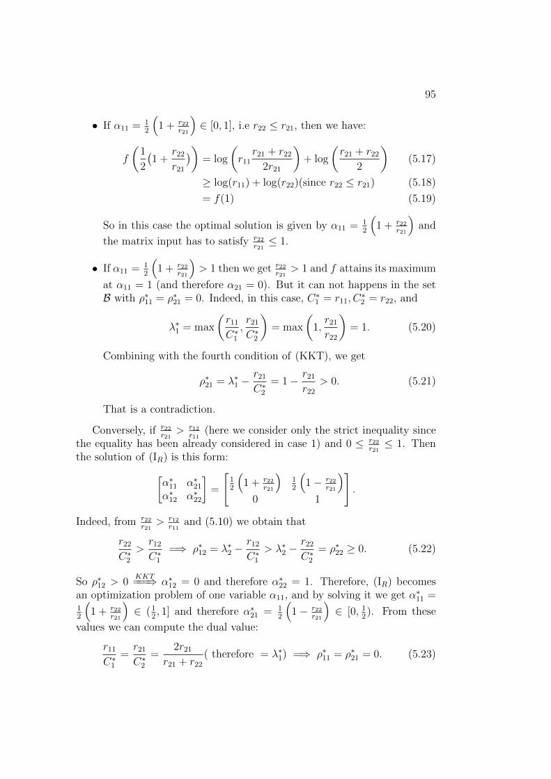
95
• If α11 = 12
(1 + r22
r21
)∈ [0, 1], i.e r22 ≤ r21, then we have:
f
(1
2
(1 +
r22
r21
))= log
(r11
r21 + r22
2r21
)+ log
(r21 + r22
2
)(5.17)
≥ log(r11) + log(r22)(since r22 ≤ r21) (5.18)
= f(1) (5.19)
So in this case the optimal solution is given by α11 = 12
(1 + r22
r21
)and
the matrix input has to satisfy r22r21≤ 1.
• If α11 = 12
(1 + r22
r21
)> 1 then we get r22
r21> 1 and f attains its maximum
at α11 = 1 (and therefore α21 = 0). But it can not happens in the setB with ρ∗11 = ρ∗21 = 0. Indeed, in this case, C∗1 = r11, C
∗2 = r22, and
λ∗1 = max
(r11
C∗1,r21
C∗2
)= max
(1,r21
r22
)= 1. (5.20)
Combining with the fourth condition of (KKT), we get
ρ∗21 = λ∗1 −r21
C∗2= 1− r21
r22
> 0. (5.21)
That is a contradiction.
Conversely, if r22r21
> r12r11
(here we consider only the strict inequality sincethe equality has been already considered in case 1) and 0 ≤ r22
r21≤ 1. Then
the solution of (IR) is this form:[α∗11 α∗21
α∗12 α∗22
]=
[12
(1 + r22
r21
)12
(1− r22
r21
)0 1
].
Indeed, from r22r21
> r12r11
and (5.10) we obtain that
r22
C∗2>r12
C∗1=⇒ ρ∗12 = λ∗2 −
r12
C∗1> λ∗2 −
r22
C∗2= ρ∗22 ≥ 0. (5.22)
So ρ∗12 > 0KKT===⇒ α∗12 = 0 and therefore α∗22 = 1. Therefore, (IR) becomes
an optimization problem of one variable α11, and by solving it we get α∗11 =12
(1 + r22
r21
)∈ (1
2, 1] and therefore α∗21 = 1
2
(1− r22
r21
)∈ [0, 1
2). From these
values we can compute the dual value:
r11
C∗1=r21
C∗2=
2r21
r21 + r22
( therefore = λ∗1) =⇒ ρ∗11 = ρ∗21 = 0. (5.23)

96 CHAPTER 5. DISCUSSION ABOUT CONTINUITY OF STO1
Conclusion for case 2: The region in this case is equal to the regiondefined by r22
r21≥ r12
r11and 0 ≤ r22
r21≤ 1. On the triangle defined by r22
r21> r12
r11(strictly inequality here) and 0 ≤ r22
r21≤ 1, the solution is unique, and is given
by
α11 =1
2
(1 +
r22
r21
).
The formula shows the continuity on the interior of the triangle. In thisregion, except on the segment defined by r22
r21= 1 ≥ r12
r11, the solution is not
integer.Case 3: Similar to case 2, if α∗12 = 1, then R has to satisfy: 0 ≤ r12
r11≤ 1
and r12r11≥ r22
r21. When 0 ≤ r12
r11≤ 1 and r12
r11> r22
r21, the solution is unique and
given by [α∗11 α∗21
α∗12 α∗22
]=
[12
(1− r12
r11
)12
(1 + r12
r11
)1 0
].
Conclusion for case 3: The region in this case is equal to the region definedby r22
r21≤ r12
r11and 0 ≤ r12
r11≤ 1. On the triangle defined by r22
r21< r12
r11and
0 ≤ r12r11≤ 1, the solution is unique, and is given by
α11 =1
2
(1− r12
r11
). (5.24)
The formula shows the continuity on the interior of the triangle. In thisregion, except on the segment r12
r11= 1 ≥ r22
r21, the solution is not integer.
The above analysis characterizes the structure of the set B. Since A isthe complement of B, it contains two connected components: one defined byr12r11
> 1 and r12r11
> r22r21
; and the other one defined by r22r21
> 1 and r12r11
< r22r21
.Recall that on A we have: #I1(R) = 1, i.e at time slot 1 only one user
gets a full allocation while the other one gets nothing. There are thus onlytwo options: either (α∗11, α
∗21) = (0, 1) or (α∗11, α
∗21) = (1, 0). As stated in
Proposition 5.5.1, (α∗11, α∗21) is continuous on A. Together with the fact that
there are only two possible options for the output which is of discrete type,this implies that F must be equal to a constant (either (0, 1) or (1, 0)) ineach connected component. Therefore, to know which value of the outputcorresponds to each connected component, we just need to choose one pointin that connected component of A and solve the optimization problem forthat point.
Let use consider the first connected component of A which is defined byr12r11
> 1 and r12r11
> r22r21
. In this region, (α∗11, α∗21) = (0, 1). Indeed, let us choose
one input point in this connected component such that it satisfies r11 > 1.

97
Since either α∗11 = 0 or α∗11 = 1, we just need to compare maxO|α11=1(α12)and maxO|α11=0(α12). We have
O|α11=1 = log(r11 + α12r12) + log((1− α12)r22) := g(α12). (5.25)
This is a function of one variable α12, we have:
g′(α12) = 0⇐⇒ α12 =1− r11
1 + r12
. (5.26)
We have α12 = 1−r111+r12
< 0 since r11 > 1. Therefore the optimal α∗12 is stay inthe boundary, i.e,
maxO|α11=1 = max(O|α11=1,α12=1, O|α11=1,α12=0
)(5.27)
= max (log(r11) + log(r22),−∞) (5.28)
= log(r11) + log(r22). (5.29)
On the other hand,
O|α11=0 = log(α12r12) + log(r21 + (1− α12)r22). (5.30)
Combining with the condition r12r11
> r22r21
we obtain
O|α11=0,α12=1 = log(r12) + log(r21) (5.31)
> log(r11) + log(r22) (5.32)
= maxO|α11=1. (5.33)
This implies α∗11 = 0 in this case.Similarly, for the connected component defined by r22
r21> 1 and r12
r11< r22
r21we
have α∗11 = 1.
Conclusion:
• B contains the box restricted by 0 ≤ r12r11≤ 1 and 0 ≤ r22
r21≤ 1 and the
line r22r21
= r12r11
. A is the remaining.
• As proven in Proposition 5.5.1, F is continuous that onA, and moreover
– on the region defined by r12r11
> 1 and r12r11
> r22r21
, α∗11 = 0,
– on the region defined by r22r21
> 1 and r12r11
< r22r21
, α∗11 = 1.
Combining with the formulas obtained in the three above cases for theset B, we can see that the set of all discontinuities is the line r12
r11= r22
r21.
• (α∗11, α∗21) is uniquely defined except on the line r22
r21= r12
r11.
Figure 5.8 illustrates Proposition 5.5.5 by showing the different regionsand the optimal solution in each region.

98 CHAPTER 5. DISCUSSION ABOUT CONTINUITY OF STO1
Figure 5.9: Choosing solution in the line to obtain a continuous function in2-dimension.
5.5.3 Proposed method to obtain a continuous func-tion
In the above 2-dimension case, the set of discontinuities (the line) is a smallset in the sense that it has Lebesgue measure equal to 0. However it makesthe model difficult to learn when the matrix input is near the line, since itoscillates between α∗1 = (0, 1) and α∗1 = (1, 0) out side the box and oscillatesbetween α∗1 = (1
2− 1
2x, 1
2+ 1
2x) and α∗1 = (1
2+ 1
2y, 1
2− 1
2y) (x ≈ y and
x, y > 0) inside the box. In order to make a continuous function, we proposeto choose the optimal allocation when it is not unique as illustrated in Figure5.9. Define H(a1, a2) = (max(a1, a2),min(a1, a2)). If we choose the solutionas described in Figure 5.9, H ◦F is a continuous function. It is reasonable tohope that learning H ◦F is easier than learning the non-continuous functionF directly.
In general, choosing an order in order to have a continuous function isnot an easy task, since to choose an order as above we actually have to solvean optimization problem. We instead propose several heuristic orders, thatare either based on current rate, based on the ratio between current rate andcumulative (the PF index), or based on (PS)2S index. The numerical resultsof these heuristic orders are shown in Section 5.6.4.
5.5.4 Loss, DFNN architecture, initial parameters andoptimizer
We will try several different loss functions and architectures and comparethem in the numerical section. The initial paramters (weights) of the DFNN

5.6. NUMERICAL COMPARISONS 99
will be chosen as proposed in [38], which allows the initial parameters tobe not too big and not too small. The optimizer is Adam first introducedin [34] which is a stochastic first-order gradient-based optimization. Theconvergence of Adam is proven in [58].
5.6 Numerical Comparisons
In this section, we do simulations to evaluate the influence of many factors onthe behavior of the DFNN model (loss functions, architecture of the DFNN,ordering scheme and learning with dual value). We use the keras library [16]to implement our code and follow the instructions in [15].
There are actually a lot of factors that can have an impact on the be-havior of the learning procedure such as: initial learning rate, learning ratedecay, optimizer, initial weight, number of parameters, activation functionsin layers... Here we are not able to justify all our choices, but we focus onthe factors which have the most significant impact on the learning algorithmin our opinion. The initial learning rate is chosen equal to 0.0015 and aftereach epoch, this learning rate decays by a factor 0.998.
5.6.1 An Unified Data Generator for Comparison
To support the comparisons in this section, the data (both for training andvalidation) is generated as follows. The number of users is generated ran-domly from 0 to KM = 10. The sojourn time of each user is generated in(0, 400) seconds. This value could of course be increased, but here in order toreduce the learning time and be able to make many comparisons, we consideronly small scenarios. The transmission rate in each small slot is generatedrandomly between 0 and 5 ∗ δ/∆. The rate we use for evaluating in SUMOscenarios are given by
r(x) = η(1 + κ e−d(x,BS)/σ
), (5.34)
where d(x,BS) is the distance from position x to the BS, and η representsthe noise level. For the SUMO scenarios in Section 5.6.5, we use κ = 3,σ = 100 and η ∼ Uniform(0.7, 1.3). The others parameters are equal toJ = 10,∆ = 1 s, δ = 2 ms.
5.6.2 Comparison of different DFNN architectures
In this part, we will consider 4 different architectures of the DFNN modeland compare their performances. For the 4 models, the activation function

100 CHAPTER 5. DISCUSSION ABOUT CONTINUITY OF STO1
Figure 5.10: Model 1 architecture.
used in hidden layers is the relu function, whereas the output layer uses thesoftmax function since we want the sum of the allocations to be equal to 1.In this comparison, we use the same loss function for all models, the huberloss [74].
Model 1
The first model used in this section contains 2 layers which are 1 hidden layerand 1 output layer. The hidden layer contains 500 units, and in total themodel has 67, 510 parameters. The architecture of this model is illustratedin Figure 5.10.
Model 2
As the first model, the second model contains 2 layers: 1 hidden layer and1 output layer. However, the hidden layer contains 1000 units, and in totalthe model has 135, 010 parameters. We take the same number of layers as inmodel 1 (but more units in hidden layers) in order to compare whether it isbetter to have more parameters.
Model 3
As the two previous models, the third model contains 2 layers (1 hiddenlayer and 1 output layer). The hidden layer contains 100 units, and we have13, 510 parameters in total. We take the same number of layers as in model

5.6. NUMERICAL COMPARISONS 101
1 (but fewer units in hidden layers) to compare whether it is better to havefewer parameters.
Model 4
The last model contains 10 layers which are 9 hidden layers and 1 outputlayer. Each hidden layer contains 82 units, and in total the model contains67, 496 parameters. We take a model has almost the same number of param-eters with the model 1, to compare whether it is better to have more layersor fewer layers.
Remark 5.6.1 (Joint power control and channel allocation). For the jointpower control and channel allocation problem, we still compare the four abovemodels except that the output layer of each model will be modified since itincludes not only the channel allocation but also the power.
Figure 5.11a illustrates the loss of the 4 models on training and validationdata. Figure 5.11b plots loss and absolute error of the 4 models on the sameaxis on validation set. The same quantities but for the problem of joint powercontrol and channel allocation are shown in Figure 5.12a and Figure 5.12brespectively.
From these figures, we observe that for the model without power control:
• Having almost the same number of parameters, model 1 with few layersis better than model 4.
• Having the same layers, model 1 and model 2 with more parametersare better than model 3.
• Model 1 and model 2 behave similarly and have the same number oflayers. However model 1 has less parameters than model 2 so it is lesscostly from a computational point of view. Therefore from now on weshall use model 1 for other comparisons in the sequel.
For the model with power control:
• Having almost the same number of parameters, model 1 with few layersis slightly better than model 4, but the difference is quite small in thiscase.
• Having the same layers, model 1, 2 and 3 are almost the same butmodel 3 has fewer parameters.

102 CHAPTER 5. DISCUSSION ABOUT CONTINUITY OF STO1
(a) Loss on training set and validation set of each model
(b) Plot on same axis for loss and absolute error on validation set of all the fourmodels
Figure 5.11: Comparison of the 4 DFNN models.

5.6. NUMERICAL COMPARISONS 103
(a) Loss on training set and validation set of each model
(b) Plot on same axis for loss and absolute error on validation set of all the fourmodels
Figure 5.12: Comparison of the 4 DFNN models for the joint power controland channel allocation problem.

104 CHAPTER 5. DISCUSSION ABOUT CONTINUITY OF STO1
(a) Absolute error on training and validation set of the two losses
(b) Plot on same axis of the absolute error on validation of the two losses
Figure 5.13: Comparison of Loss functions.

5.6. NUMERICAL COMPARISONS 105
5.6.3 Comparisons of different loss functions
To compare the quality of the learning model obtained using different lossfunctions, we use the same model, that is model 1. Figure 5.13 presents theresults obtained with the huber loss [74], with the sum of binary cross-entropy[72] and dice loss (which equals to 1− dice coefficient [73]). The second lossfunction is denoted by bce dice loss. From the figures, the bce dice lossfunction is better in this case. So for the next comparisons, we shall usemodel 1 and bce dice loss.
5.6.4 Comparisons of different ordering schemes
As mentioned above, we shall use model 1 and bce dice loss for this compar-ison. We compare the results obtained with 4 different ordering schemes: noorder, current rate order, PF order and (PS)2S order. Figure 5.14 presentsour numerical results. (PS)2S order seems the best one among the 4 orderingschemes.
5.6.5 Comparisons of learning the channel allocationagainst learning dual values
In this section, we compare learning dual values against learning directly theallocation. As mentioned above, for learning the allocation, we use model 1and bce dice loss. Since the value of the dual need not lie in [0, 1], we cannotuse and a softmax activation function in the output layer and bce dice lossdirectly. We shall normalize the dual values by dividing each element by thesum of all elements before fitting it into the DFNN model. This normalizationis continuous, therefore we still have a continuous mapping. Finally, we canuse sofmax and bce dice loss. The absolute error of the different learningschemes are shown in Figure 5.15.
Since the values of the allocation and the dual are different, it is notpossible to compare the losses or absolute errors directly as before. We shallinstead compare three different learning schemes (learning allocation withoutorder, learning allocation with (PS)2S order and learning the dual values) ontwo different scenarios created with SUMO. The first scenario contains 244users and lasts in 61.7 minutes inside the coverage of one BS. The map ofthis scenario is shown in Figure 5.2. The results obtained with the differentlearning schemes on this scenario are shown in Figure 5.17. The secondscenario contains 214 users and lasts 62.4 minutes. The map of this scenariois shown in Figure 5.16. The results obtained with the different learningschemes on this scenario are shown in Figure 5.18.

106 CHAPTER 5. DISCUSSION ABOUT CONTINUITY OF STO1
(a) Loss on training and validation set
(b) Plot on same axis of the loss and absolute error on validation set
Figure 5.14: Comparison of 4 different types of ordering schemes.
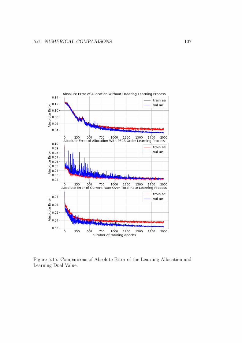
5.6. NUMERICAL COMPARISONS 107
Figure 5.15: Comparisons of Absolute Error of the Learning Allocation andLearning Dual Value.

108 CHAPTER 5. DISCUSSION ABOUT CONTINUITY OF STO1
Figure 5.16: Duroux, one BS type LTE1800, operator SFR. The actual sizeis around 350*500m.
We see that learning dual values outperforms the two other learningschemes: it is more stable, provides a better allocation and it convergesfaster than learning directly the allocation without any ordering scheme. Itcosts the same time for prediction as the other two approaches since theyare using the same architecture (i.e, model 1). However learning directlyallocation with a user ordering scheme requires to compute in addition theorder, which consumes more computing time than the other two approaches.
5.7 Computing times
The computing time of STO1 depends on the convex optimization solverused, whereas the learning algorithm has only to feed the DFNN model withthe input matrix. We consider the same setting as in Section 5.6.2, that isK = 10 (there are 10 users in the system) and the short term horizon isJ = 10 seconds. For these values, the average computing time of mosek isaround 43.7 ms, whereas the prediction with the DFNN model (model 1)takes only 0.65 ms on average. These computing times are averages over10000 samples, and both are measured on a machine using GPU (graphicsprocessing unit) which allows computing many calculations in parallel.

5.8. DISCUSSION ONA REINFORCEMENT LEARNING BASED APPROACH FOR LEARNINGOPTIMAL POLICY109
250 500 750 1000 1250 1500 1750 2000number of learning epochs
6.90
6.85
6.80
6.75
6.70
6.65
aver
age
tota
l util
ity
STO1Learning Allocation No OrderLearning Allocation PF2S OrderLearning Dual Value(PF)2SPF
Figure 5.17: Comparisons of evaluated on Carmes scenario created by SUMOof Allocation and Dual Value.
5.8 Discussion on a reinforcement learning
based approach for learning Optimal Pol-
icy
In this section, we shall discuss about learning the optimal policy by usingDeep Q Network (DQN) learning. The background of DQN is recalled in2.5.3. To do that, it requires the state of the system follows a Markov process.To simplify, we consider a straight road only in this discussion.
Assume that every time-slot, at most one arrival enters the system andthe new arrival comes independently and with probability p. Now we definethe tuple of state, action, reward one-step and transition matrix to get aMarkov Decision Problem (MDP).
State and action: A state is a matrix 2-D size N × 2 (N is number ofsmall slots in coverage range), where:
• first row is vector of 0 and 1 to indicate whether there is a car in thatplace or not.
• second row is a vector of corresponding cumulative data.

110 CHAPTER 5. DISCUSSION ABOUT CONTINUITY OF STO1
400 600 800 1000 1200 1400 1600 1800 2000number of learning epochs
7.55
7.50
7.45
7.40
7.35
7.30
aver
age
tota
l util
ity
STO1Learning Allocation No OrderLearning Allocation PF2S OrderLearning Dual Value(PF)2SPF
Figure 5.18: Comparisons of evaluated on Duroux scenario created by SUMOof Allocation and Dual Value.
N slotsCoverage range of the BS
Rate curve
Arrivals 1 slot
Figure 5.19: Straight road.

5.8. DISCUSSION ONA REINFORCEMENT LEARNING BASED APPROACH FOR LEARNINGOPTIMAL POLICY111
cumulative data of every user is initialized with d0 where d0 is a very smallnumber to avoid log of zero. If there is no user in a place, the cumulativedata for that place is filled by d0 by convention. Here the future rate is nottaken into account in the state, but the Q function is expected to learn itby learning the data rate map during iterations, since here we restrict thelearning on a specific map that is a straight road. So, in this setting, aftergetting the Q function, the algorithm will work only for this specific map (thisis different from the supervised learning that was done for STO1 where themodel is trained on a general system and therefore will work on an arbitrarynetwork).
Action space A = {1, 2, ..., N}, if action a = k it means the car in placek is chosen.
Reward one-step is defined:
R(X, a) = log(xa,2 + r(a))− log(xa,2),
where r is the rate function, r(a) means rate at position a and xa,2 is theelement in position a of the second row of the matrix X.
Transition matrix: As a new arrival can enter with probability p andthe vector of cumulative data can be changed, if we are currently in stateX = (xi,j)i=1,2,j=1,2,...N , it can be turned into new state as follows:
• with probability p it goes to state Y = (yi,j)i=1,2,j=1,2,...N where:
? y1,1 = 1, y1,2 = d0,
? and yi+1,1 = xi,1, yi+1,2 = xi,2 if user in place i is not chosen andotherwise yi+1,2 = xi,2 +r(i) where r(i) stands for the rate at placei, for all i = 2, 3, .., N − 1.
• with probability 1− p it goes to state Y = (yi,j)i=1,2,j=1,2,...N where:
? y1,1 = 0, y1,2 = d0,
? and yi+1,1 = xi,1, yi+1,2 = xi,2 if user in place i is not chosen andotherwise yi+1,2 = xi,2 +r(i) where r(i) stands for the rate at placei, for all i = 2, 3, .., N − 1.
Objective: We want to build a potential function, which takes state Xas an input and gives us suggestion for the good action a, that is Q-functionQ(X, a).
By value iteration, we get the optimal solution for this MDP when Nsmall. In value iteration, we need to store the table of the value function ofall states which is not possible when N large. One of the methods people use

112 CHAPTER 5. DISCUSSION ABOUT CONTINUITY OF STO1
Figure 5.20: Deep Q learning comparing to Q learning and Optimal Policy,N = 3, p = 0.5, discounted factor γ = 0.9.
to deal with large state space is to learn Q function instead of V by usingfunction approximation.
Fig. 5.20 illustrates the comparison of three algorithms: Optimal Policygot by value iteration, Q learning and Deep Q learning. In that numericalresult, in each episode, we do the same 2000 iterations both for DQN andQ learning. Here we can see even with N = 3 it takes so long time (75episodes) to see the convergence of the DQN and DQN even converges quitefar from the true value got by Value Iteration. There are two disadvantages ofthis method. Firstly, when N increases, the size of the state-space increasesexponentially. In fact, N should be of the order of thousands, which makes avery huge state space. Secondly, by the way we defined the model above, wedo not have a terminal state. Those two things may make both of Q learningand Deep Q learning more difficult to converge to the true value.
5.9 Summary and Discussion
We have proposed machined learning based method for learning one of ourheuristics (the STO 1) introduced in chapter 3 and chapter 4 in order to

5.9. SUMMARY AND DISCUSSION 113
produce an approximate solution which can process many times faster. Wehave proved that the primal values used in STO 1 are not continuous in theinput. We then proposed some ordering methods to reduce the discontinuityof the primal values. We also proved that the dual values are continuous,we thus proposed to learn the duals instead of the primals. The orderingmethods help the model converges faster but not always increases the per-formance, while the dual method helps the model learn faster and performbetter. We also presented another approach using reinforcement learning.Different from Supervise Learning approach, Reinforcement Learning worksfor specific topology maps, needs long time to converge even for very smallscenario.
The way we define the state for the DFNN here makes the model can learnon a general network, not only for specific topology map. There are severaldirections of research that can be investigated to improve the learning, suchas better generator of data, better loss function, better architecture DFNNmodel, and other thing such as optimizer, learning rate, etc.

114 CHAPTER 5. DISCUSSION ABOUT CONTINUITY OF STO1

Chapter 6
Discussion and Future Works
In this thesis, we have investigated two different resource allocation problems.The first one deals with the channel allocation to vehicular users in cellularnetworks, whereas the second one is the joint channel allocation and powercontrol problem in cellular networks. For each problem, we have proposedtwo heuristic algorithms which assume that the mean future rates of vehic-ular users can be predicted over a few seconds. The main originality of ouralgorithms is that they combine this information on future radio conditionswith the information on present channel channel conditions to compute whatshould be the optimal allocation in the next few seconds. This is done bysolving a relaxed version of a utility maximization problem over a short-termhorizon. This extra-knowledge on future allocations can then be used forimproved online channel allocation and/or power control. Our algorithmscan be applied to general network topologies and are shown numerically tooutperform other existing algorithms. In the last part of the thesis , we havealso presented a machine learning-based method for obtaining approximatealgorithms that mimic our resource allocation algorithms but can be runmany times faster. Numerical results show that the approximate algorithmsare well suited to real-time processing and that the degradation of the chan-nel allocation quality is very small. Below, we discuss some open researchdirections that could be followed to extend our work.
There are several directions in which our work can be extended. Oneavenue is to implement a centralized and coordinated version for the multipleBSs case of our heuristics. On the analytical side, obtaining sub-optimalitybounds for our heuristics would also be worth investigating. It would be alsointeresting to study the robustness of our heuristic algorithms with respectto errors in future information. The dual-decomposition methods presentedin [54] could also be applied to get another heuristic algorithm but with apenalty term instead of the average power constraint.
115
116 CHAPTER 6. DISCUSSION AND FUTURE WORKS
For both problems, it would be interesting to extend our work to differentutility functions and to problems in which users have QoS requirements (e.g.,latency or jitter). We also note that the joint channel allocation and powercontrol problem could be studied on the up-link, and that similar algorithmscould be investigated for the opportunistic utility model.
Finally, another interesting extension would be to consider settings inwhich the information available on users is heterogeneous. We particularlyhave in mind the two following settings:
• a setting in which future information is not available for some userswhich are unpredictable. For instance, the future positions of pedes-trians are probably more difficult to predict than those of cars movingalong a highway. An idea that could be applied in this case is to applyPF scheduling for those ”unpredictable” users, and to use our heuristicsfor the other users,
• a setting in which the positions of some users can be predicted withhigher accuracy and over a longer time period than those of the otherusers. For example, compared to the individual users, the public trans-ports (bus, tram, metro,...) may be easier to predict in longer timeperiod and with higher accuracy. Another example is the case of vehic-ular users agreeing to share the information on their itinerary. An ideathat could be applied in these situations is that the estimated futurerate can be equal to expectation over all possibilities of the future pathprediction.

Bibliography
[1] Press release: Local clouds for greater road safety - joint de-velopment project between bosch, nokia, and deutsche telekom.2016. https://www.bosch-presse.de/pressportal/de/en/
local-clouds-for-greater-road-safety-63296.html.
[2] Just one autonomous car will use 4,000 gb of data/day. December2016. http://www.networkworld.com/article/3147892/internet/
one-autonomous-car-will-use-4000-gb-of-dataday.html.
[3] H. Abou-zeid, H. S. Hassanein, and N. Zorba. Long-term fairness inmulti-cell networks using rate predictions. In 2013 7th IEEE GCC Con-ference and Exhibition (GCC), pages 131–135, Nov 2013.
[4] M. H. Ahmed, O. Dobre, and R. Almatarneh. Analytical evaluation ofthe performance of proportional fair scheduling in ofdma-based wirelesssystems. Journal of Electrical and Computer Engineering, 2012, 08 2012.
[5] A. Anand and G. Veciana. A whittle’s index based approach for qoeoptimization in wireless networks. ACM SIGMETRICS PerformanceEvaluation Review, 46:39–39, 06 2018.
[6] R. Atallah, C. Assi, and M. Khabbaz. Deep reinforcement learning-based scheduling for roadside communication networks. pages 1–8, 052017.
[7] H. J. Bang, T. Ekman, and D. Gesbert. Channel predictive propor-tional fair scheduling. IEEE Transactions on Wireless Communications,7(2):482–487, February 2008.
[8] D. P. Bertsekas. Dynamic Programming and Optimal Control. AthenaScientific, 2nd edition, 2000.
[9] V. Borkar and S. Pattathil. Whittle indexability in egalitarian processorsharing systems. Annals of Operations Research, 08 2017.
117

118 BIBLIOGRAPHY
[10] S. Borst. User-level performance of channel-aware scheduling algorithmsin wireless data networks. IEEE/ACM Transactions on Networking,13(3):636–647, June 2005.
[11] S. Borst, N. Hegde, and A. Proutiere. Mobility-driven scheduling inwireless networks. In IEEE INFOCOM 2009, pages 1260–1268, April2009.
[12] T. Bu, L. Li, and R. Ramjee. Generalized proportional fair schedul-ing in third generation wireless data networks. In Proceedings IEEEINFOCOM 2006. 25TH IEEE International Conference on ComputerCommunications, pages 1–12, 2006.
[13] P. Chandur, R. M. Karthik, and K. M. Sivalingam. Performance evalua-tion of scheduling algorithms for mobile wimax networks. In 2012 IEEEInternational Conference on Pervasive Computing and CommunicationsWorkshops, pages 764–769, March 2012.
[14] M. Chiang, P. Hande, T. Lan, and C. W. Tan. Power control in wirelesscellular networks. Foundations and Trends R© in Networking, 2(4):381–533, 2008.
[15] F. Chollet. Deep Learning with Python. Manning Publications Co.,USA, 1st edition, 2017.
[16] F. Chollet et al. Keras. https://github.com/fchollet/keras, 2015.
[17] L. Condat. Fast projection onto the simplex and the l1 ball. Math.Program., 158:575–585, 2016.
[18] G. Cybenko. Approximation by superpositions of a sigmoidal function.Mathematics of Control, Signals and Systems, 2(4):303–314, 1989.
[19] E. Dahlman, S. Parkvall, and J. Skold. 4G LTE-Advanced Pro and TheRoad to 5G (Third Edition). Academic Press, third edition edition, 2016.
[20] S. Diamond and S. Boyd. CVXPY: A Python-embedded modeling lan-guage for convex optimization. Journal of Machine Learning Research,17(83):1–5, 2016.
[21] C. B. Do. Convex optimization overview (cnt’d). CS229 Lecture notes,November 2009.
[22] R. Eghbali and M. Fazel. Worst case competitive analysis of onlinealgorithms for conic optimization. CoRR, abs/1611.00507, 2016.

BIBLIOGRAPHY 119
[23] I. Goodfellow, Y. Bengio, and A. Courville. Deep Learning. MIT Press,2016. http://www.deeplearningbook.org.
[24] K. Gregor and Y. LeCun. Learning fast approximations of sparse coding.In Proceedings of the 27th International Conference on InternationalConference on Machine Learning, ICML’10, page 399–406, Madison,WI, USA, 2010. Omnipress.
[25] D. Grewe, M. Wagner, M. Arumaithurai, I. Psaras, and D. Kutscher.Information-centric mobile edge computing for connected vehicle envi-ronments: Challenges and research directions. In Proceedings of theWorkshop on Mobile Edge Communications, MECOMM ’17, page 7–12,New York, NY, USA, 2017. Association for Computing Machinery.
[26] J. M. Holtzman. Asymptotic analysis of proportional fair algo-rithm. 12th IEEE International Symposium on Personal, Indoorand Mobile Radio Communications. PIMRC 2001. Proceedings (Cat.No.01TH8598), 2:F–F, 2001.
[27] K. Hornik. Approximation capabilities of multilayer feedforward net-works. Neural Networks, 4(2):251 – 257, 1991.
[28] K. Hornik, M. Stinchcombe, and H. White. Multilayer feedforward net-works are universal approximators. Neural Networks, 2(5):359 – 366,1989.
[29] J. Huang, V. Subramanian, R. Agrawal, and R. Berry. Downlinkscheduling and resource allocation for ofdm systems. IEEE Transac-tions on Wireless Communications, 8:288–296, 01 2009.
[30] R. Hussain, J. Son, H. Eun, S. Kim, and H. Oh. Rethinking vehicularcommunications: Merging vanet with cloud computing. In 4th IEEEInternational Conference on Cloud Computing Technology and ScienceProceedings, pages 606–609, 2012.
[31] A. Karbassi and M. Barth. Vehicle route prediction and time of ar-rival estimation techniques for improved transportation system man-agement. In IEEE IV2003 Intelligent Vehicles Symposium. Proceedings(Cat. No.03TH8683), pages 511–516, 2003.
[32] F. Kelly. Charging and rate control for elastic traffic. European Trans-actions on Telecommunications, 8(1):33–37, 1997.
120 BIBLIOGRAPHY
[33] F. P. Kelly, A. K. Maulloo, and D. K. H. Tan. Rate control for com-munication networks: shadow prices, proportional fairness and stability.Journal of the Operational Research Society, 49(3):237–252, Mar 1998.
[34] D. Kingma and J. Ba. Adam: A method for stochastic optimization.International Conference on Learning Representations, 12 2014.
[35] A. Kolmogorov. On the representation of continuous functions of manyvariables by superposition of continuous functions of one variable andaddition. Dokl. Akad. Nauk SSSR, 114(5):953–956, 1957.
[36] J. Krumm. A markov model for driver turn prediction. In Society of Au-tomotive Engineers (SAE) 2008 World Congress, April 2008. SAE 2008World Congress, April 2008. Lloyd L. Withrow Distinguished SpeakerAward.
[37] H. J. Kushner and P. A. Whiting. Convergence of proportional-fairsharing algorithms under general conditions. IEEE Transactions onWireless Communications, 3(4):1250–1259, July 2004.
[38] Y. Lecun, L. Bottou, G. Orr, and K.-R. Muller. Efficient backprop. 082000.
[39] J. Lee, R. R. Mazumdar, and N. B. Shroff. Opportunistic power schedul-ing for dynamic multi-server wireless systems. IEEE Trans. WirelessCommunications, 5(6):1506–1515, 2006.
[40] C. Li and M. J. Neely. Network utility maximization over partiallyobservable markovian channels. Perform. Evaluation, 70(7-8):528–548,2013.
[41] E. Liu and K. K. Leung. Proportional fair scheduling: Analytical insightunder rayleigh fading environment. In 2008 IEEE Wireless Communi-cations and Networking Conference, pages 1883–1888, 2008.
[42] P. A. Lopez, M. Behrisch, L. Bieker-Walz, J. Erdmann, Y.-P. Flotterod,R. Hilbrich, L. Lucken, J. Rummel, P. Wagner, and E. Wießner. Mi-croscopic traffic simulation using sumo. In The 21st IEEE InternationalConference on Intelligent Transportation Systems. IEEE, 2018.
[43] R. Margolies, A. Sridharan, V. Aggarwal, R. Jana, N. K. Shankara-narayanan, V. A. Vaishampayan, and G. Zussman. Exploiting mobilityin proportional fair cellular scheduling: Measurements and algorithms.IEEE/ACM Trans. Netw., 24(1):355–367, Feb. 2016.

BIBLIOGRAPHY 121
[44] A. Mesbah. Stochastic model predictive control: An overview and per-spectives for future research. IEEE Control Systems Magazine, 36(6):30–44, Dec 2016.
[45] J. Mo and J. Walrand. Fair end-to-end window-based congestion control.IEEE/ACM Transactions on Networking, 8(5):556–567, 2000.
[46] S. Moharir and S. Shakkottai. Maxweight versus backpressure: Routingand scheduling in multichannel relay networks. IEEE/ACM Transac-tions on Networking, 23(5):1584–1598, Oct. 2015.
[47] H. Montanelli and H. Yang. Error bounds for deep relu networks usingthe kolmogorov–arnold superposition theorem, 2019.
[48] K. Navaie and H. Yanikomeroglu. Fairness of resource allocation incellular networks : a survey. 2005.
[49] M. J. Neely. Energy optimal control for time-varying wireless networks.IEEE Transactions on Information Theory, 52(7):2915–2934, 2006.
[50] M. J. Neely. Order optimal delay for opportunistic scheduling in multi-user wireless uplinks and downlinks. IEEE/ACM Transactions on Net-working, 16(5):1188–1199, Oct 2008.
[51] N. Nguyen, O. Brun, and B. Prabhu. An algorithm for improvedproportional-fair utility for vehicular users. The 25th International Con-ference on Analytical and Stochastic Modelling Techniques and Applica-tions ASMTA-2019, May 2019.
[52] N. Nguyen, O. Brun, and B. Prabhu. Joint downlink power controland channel allocation based on a partial view of future channel con-ditions. The 15th Workshop on Resource Allocation, Cooperation andCompetition in Wireless Networks, June 2020.
[53] T. T. N. Nguyen, U. Ayesta, and B. J. Prabhu. Scheduling users indrive-thru internet : a multi-armed bandit approach. 2019.
[54] D. P. Palomar and Mung Chiang. A tutorial on decomposition methodsfor network utility maximization. IEEE Journal on Selected Areas inCommunications, 24(8):1439–1451, 2006.
[55] M. L. Puterman. Markov Decision Processes: Discrete Stochastic Dy-namic Programming. John Wiley & Sons, Inc., New York, NY, USA,1st edition, 1994.

122 BIBLIOGRAPHY
[56] B. Radunovic and J. Le Boudec. A unified framework for max-minand min-max fairness with applications. IEEE/ACM Transactions onNetworking, 15(5):1073–1083, 2007.
[57] B. Radunovic and J. Le Boudec. A unified framework for max-minand min-max fairness with applications. IEEE/ACM Transactions onNetworking, 15(5):1073–1083, 2007.
[58] S. J. Reddi, S. Kale, and S. Kumar. On the convergence of adam andbeyond. CoRR, abs/1904.09237, 2019.
[59] S. Shenker. Fundamental design issues for the future internet. IEEEJournal on Selected Areas in Communications, 13(7):1176–1188, 1995.
[60] H. SHI, R. V. Prasad, E. Onur, and I. G. M. M. Niemegeers. Fairnessin wireless networks:issues, measures and challenges. IEEE Communi-cations Surveys Tutorials, 16(1):5–24, 2014.
[61] A. L. Stolyar. Maxweight scheduling in a generalized switch: Statespace collapse and workload minimization in heavy traffic. Ann. Appl.Probab., 14(1):1–53, 02 2004.
[62] V. G. Subramanian, R. A. Berry, and R. Agrawal. Joint schedulingand resource allocation in CDMA systems. IEEE Trans. Inf. Theory,56(5):2416–2432, 2010.
[63] H. Sun, X. Chen, Q. Shi, M. Hong, X. Fu, and N. D. Sidiropoulos.Learning to optimize: Training deep neural networks for wireless re-source management. CoRR, abs/1705.09412, 2017.
[64] S. Sun, W. Chen, L. Wang, X. Liu, and T.-Y. Liu. On the depth of deepneural networks: A theoretical view. In Proceedings of the ThirtiethAAAI Conference on Artificial Intelligence, AAAI’16, page 2066–2072.AAAI Press, 2016.
[65] R. S. Sutton and A. G. Barto. Introduction to Reinforcement Learning.MIT Press, Cambridge, MA, USA, 1st edition, 1998.
[66] L. Tan, Z. Zhu, F. Ge, and N. Xiong. Utility maximization resourceallocation in wireless networks: Methods and algorithms. IEEE Trans-actions on Systems, Man, and Cybernetics: Systems, 45(7):1018–1034,July 2015.

BIBLIOGRAPHY 123
[67] L. Tassiulas and A. Ephremides. Stability properties of constrainedqueueing systems and scheduling policies for maximum throughput inmultihop radio networks. IEEE Transactions on Automatic Control,37(12):1936–1948, Dec 1992.
[68] L. Tassiulas and A. Ephremides. Dynamic server allocation to paral-lel queues with randomly varying connectivity. IEEE Transactions onInformation Theory, 39(2):466–478, March 1993.
[69] D. Tse and P. Viswanath. Fundamentals of Wireless Communication.Cambridge University Press, 2005.
[70] Q. Wang, P. Fan, and K. B. Letaief. On the joint v2i and v2v schedul-ing for cooperative vanets with network coding. IEEE Transactions onVehicular Technology, 61(1):62–73, 2012.
[71] C. Wiesner, M. Ruf, D. Sirim, and G. Klinker. Visualisation of theelectronic horizon in head-up-displays. pages 87–89, 09 2016.
[72] Wikipedia. Cross entropy. 20 June 2020. https://en.wikipedia.org/wiki/Cross_entropy.
[73] Wikipedia. Sorensen dice coefficient. 28 July 2020. https://en.
wikipedia.org/wiki/S%C3%B8rensen%E2%80%93Dice_coefficient.
[74] Wikipedia. Huber loss. 29 May 2020. https://en.wikipedia.org/
wiki/Huber_loss.
[75] Wikipedia. Supervised learning. 5 July 2020. https:
//en.wikipedia.org/wiki/Supervised_learning#How_supervised_
learning_algorithms_work.
[76] Wikipedia. Activation function. 7 July 2020. https://en.wikipedia.org/wiki/Activation_function.
[77] S. Xu, G. Zhu, C. Shen, Y. Lei, and Z. Zhong. Utility-based resourceallocation in high-speed railway wireless networks. EURASIP Journalon Wireless Communications and Networking, 2014(1):68, Apr 2014.
[78] H. Ye, G. Y. Li, and B. F. Juang. Deep reinforcement learning basedresource allocation for v2v communications. IEEE Transactions on Ve-hicular Technology, 68(4):3163–3173, 2019.

124 BIBLIOGRAPHY
[79] Y. Yi and M. Chiang. Stochastic network utility maximisation—a trib-ute to kelly’s paper published in this journal a decade ago. EuropeanTransactions on Telecommunications, 19(4):421–442, 2008.
[80] H. Zhou, P. Fan, and J. Li. Global proportional fair scheduling fornetworks with multiple base stations. IEEE Transactions on VehicularTechnology, 60(4):1867–1879, May 2011.