Embed Size (px)
Citation preview
Proportional Resonant Control of
Three-Phase Grid-Connected Inverter
During Abnormal Grid Conditions
Ahmed Othman Althobaiti
Electrical Electronic Engineering
School of Engineering
Newcastle University
A thesis submitted for the degree of
Doctor of Philosophy
November, 2017

Proportional Resonance Control of Three-Phase Grid-Connected Inverter
I
Abstract
The development of using grid-connected three-phase inverter has augmented the standing of
realizing muted distortion along with high-quality current waveform. The standard three-phase
grid-connected inverter is the full-bridge voltage source inverter. This inverter is usually
controlled by proportional integral (PI) controller in order to ensure sinusoidal current injection
to the grid. Although the PI controller is well established and easy to use under normal grid
conditions, it leads to system instability under abnormal grid conditions. When abnormal grid
conditions are likely to occur, the control system with PI controller can be configured to include
two separate PI controllers for the positive and negative sequence components of the grid
current. However, this increases control complexity and total harmonic distortion (THD).
More recently, the proportional resonant (PR) controller started to replace PI controller in a
different application including grid-connected current control. In this thesis, a comprehensive
theoretical and experimental comparison between the PI and PR controllers is presented. The
comparison shows that the PR controller offers lower total harmonic distortion (THD) in the
current signal spectrum and is simpler to implement as it uses only the positive sequence
component of the grid current and consequently only one PR controller is needed. For these
reasons, the PR controller is adopted in this thesis.
Despite the PR controller offering enhanced functioning under abnormal grid conditions
compared to PI controller, a sudden change in the grid voltage could additionally raise the error
between the reference signal and the controlled signal which results in causing significant
divergence from its ostensible value. In this case, the performance of the conventional PR
controller will not keep up with the increase in the error which weakens controller performance.
To overcome this problem, a new design concept for controlling the current of the three-phase
grid connected inverter during normal and abnormal conditions is presented in this thesis. The
proposed technique replaces the static control parameters by adaptive control parameters based
on a look-up table. This adaptive PR, controller has been investigated and demonstrated with
different normal and abnormal grid conditions. The proposed control technique is capable of
providing low THD in the injected current even during the occurrence of abnormal grid
conditions compared with PI and PR controllers. It also achieves lower overshoot and settling
time as well as smaller steady-state error.

Proportional Resonance Control of Three-Phase Grid-Connected Inverter
II
Additionally, despite the fact that both PI and PR controllers are relatively straightforward to
tune, and are sometimes capable of dealing with many time-varying grid conditions. This
research also presented an adaptive controller tuned using advanced optimization techniques
based on particle swarm optimisation (PSO). PSO is presented to optimize the control
parameters of both PI and PR controllers for the three-phase grid-connected inverter. There are
many advantages of using PSO, such as no additional hardware being required. Thus, it can be
extended to other applications and control methods. In addition, the proposed method is a self-
tuning method and can thus be suitable for industrial applications where manual tuning is not
recommended for time and cost reasons. Simulation and experimental test were carried out to
investigate the performance of the proposed techniques. In the simulation, the system was tested
under 100 kW model using Matlab/Simulink environment. In addition, the system was also
investigated through a practical implementation of the control system using a Digital Signal
Processor (DSP) and grid-connected three-phase inverter. This practical system was
demonstrated a 300 W scaled-down prototype. As a result, the comparisons between
experimental and simulation results show the behaviour and performance of the control to be
accurately evaluated.

Proportional Resonance Control of Three-Phase Grid-Connected Inverter
III
Acknowledgements
I want to thank God (Allah), the most merciful and the most gracious, who gave me patience,
strength and help to achieve this scientific research.
First and foremost, I would like to thank Dr. Matthew Armstrong for his guidance and support,
throughout these years and for patiently reading and commenting on this thesis. I also appreciate
the input of Dr. Mohammed Elgendy throughout my time at Newcastle University for his trust,
guidance and support. Very sincere thanks are due to my friends in the UG lab, technicians and
staff.
I have not enough words to thank my ever first teachers in this life, my parents, who have been
inspiring me and pushing me forward all the way. Their prayers and blessings were no doubt
the true reason behind any success I have realized in my life.
Special thanks to my wife. Thank you for supporting me for everything, and especially I can't
thank you enough for encouraging me throughout this experience. To my beloved son Anas and
daughter Aleen, I would like to express my thanks for being such good children always cheering
me up.
I am grateful to all my family members for their kind support, endurance and encouragements,
which have given me the energy to carry on and to motivate myself towards crossing the finish
line.

Proportional Resonance Control of Three-Phase Grid-Connected Inverter
IV
To my dear father and mother
Proportional Resonance Control of Three-Phase Grid-Connected Inverter
V
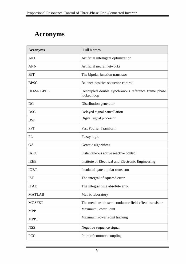
Acronyms
Acronyms Full Names
AIO Artificial intelligent optimization
ANN Artificial neural networks
BJT The bipolar junction transistor
BPSC Balance positive sequence control
DD-SRF-PLL Decoupled double synchronous reference frame phase
locked loop
DG Distribution generator
DSC Delayed signal cancellation
DSP Digital signal processor
FFT Fast Fourier Transform
FL Fuzzy logic
GA Genetic algorithms
IARC Instantaneous active reactive control
IEEE Institute of Electrical and Electronic Engineering
IGBT Insulated-gate bipolar transistor
ISE The integral of squared error
ITAE The integral time absolute error
MATLAB Matrix laboratory
MOSFET The metal-oxide-semiconductor-field-effect-transistor
MPP Maximum Power Point
MPPT Maximum Power Point tracking
NSS Negative sequence signal
PCC Point of common coupling
Proportional Resonance Control of Three-Phase Grid-Connected Inverter
VI
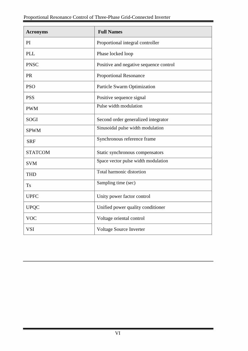
Acronyms Full Names
PI Proportional integral controller
PLL Phase locked loop
PNSC Positive and negative sequence control
PR Proportional Resonance
PSO Particle Swarm Optimization
PSS Positive sequence signal
PWM Pulse width modulation
SOGI Second order generalized integrator
SPWM Sinusoidal pulse width modulation
SRF Synchronous reference frame
STATCOM Static synchronous compensators
SVM Space vector pulse width modulation
THD Total harmonic distortion
Ts Sampling time (sec)
UPFC Unity power factor control
UPQC Unified power quality conditioner
VOC Voltage oriental control
VSI Voltage Source Inverter

Proportional Resonance Control of Three-Phase Grid-Connected Inverter
VII
Symbol
Symbol Full Names
Ia Current in phase a
Ib Current in phase b
Ic Current in phase c
Id Current in reference frame direct current (d)
Iq Current in reference frame quadratic current (q)
Iα Current in the stationary reference frame (α alpha transform)
Iβ Current in the stationary reference frame (β beta transform)
ki Integral gain of the controller
kp Proportional gain of the controller
Va Voltage in phase a
Vb Voltage in phase b
Vc Voltage in phase c
D Diode
f Frequency
L1 Inverter side inductance
L2 Grid side inductance
P Active power

Proportional Resonance Control of Three-Phase Grid-Connected Inverter
VIII
Symbol Full Names
p.u Per unit
Q Reactive power
t Time
θ Phase angle

Proportional Resonance Control of Three-Phase Grid-Connected Inverter
IX
Table of Contents
Abstract .................................................................................................................. I
Acknowledgements ............................................................................................. III
Acronyms ............................................................................................................. V
Symbol ................................................................................................................ VII
Table of Contents ................................................................................................ IX
List of Tables .................................................................................................... XIII
Table of Figures .................................................................................................... 1
Introduction ..................................................................................... 6
1.1 Background and Motivation .................................................................................................... 6
1.2 Three-phase Grid-connected Inverter..................................................................................... 9
1.3 Grid Filter Types .................................................................................................................... 11
1.4 Grid Synchronization Method ............................................................................................... 12
1.4.1 Zero Crossing Method (ZCM) ............................................................................ 13
1.4.2 Phase Locked Loop (PLL) .................................................................................. 13
1.5 Thesis Objectives ................................................................................................................... 15
1.6 Contributions of the Thesis ................................................................................................... 16
1.7 Publication ............................................................................................................................. 17
1.8 Thesis Outline: ....................................................................................................................... 17
Literature Review .......................................................................... 19
2.1 Introduction .......................................................................................................................... 19
2.2 Methods of Three-phase Current Control............................................................................. 19
2.2.1 Proportional Integral (PI) Current Controller in the Synchronous Reference
Frame 20
2.2.2 Proportional Resonance (PR) Current Controller in Stationary Reference Frame
21
2.2.3 The abc Reference Frame Current Control ........................................................ 23
2.2.4 Other Control Strategy ....................................................................................... 23
Proportional Resonance Control of Three-Phase Grid-Connected Inverter
X
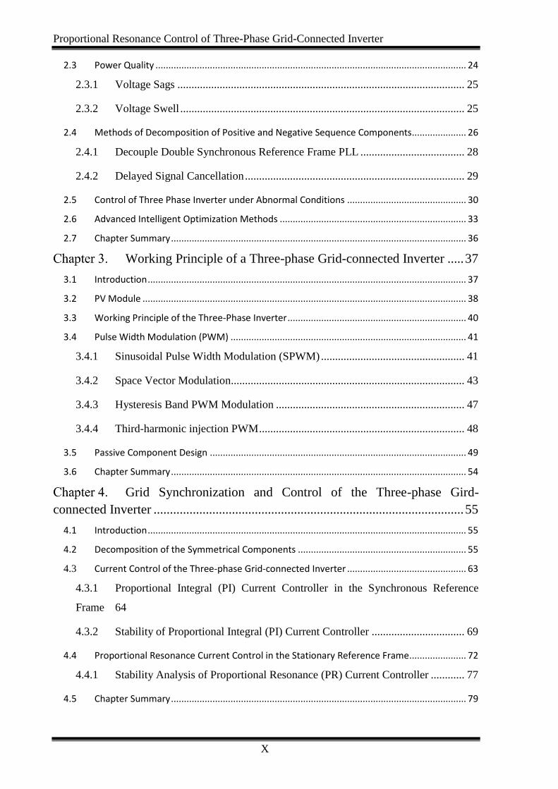
2.3 Power Quality ........................................................................................................................ 24
2.3.1 Voltage Sags ...................................................................................................... 25
2.3.2 Voltage Swell ..................................................................................................... 25
2.4 Methods of Decomposition of Positive and Negative Sequence Components ..................... 26
2.4.1 Decouple Double Synchronous Reference Frame PLL ..................................... 28
2.4.2 Delayed Signal Cancellation .............................................................................. 29
2.5 Control of Three Phase Inverter under Abnormal Conditions .............................................. 30
2.6 Advanced Intelligent Optimization Methods ........................................................................ 33
2.7 Chapter Summary .................................................................................................................. 36
Working Principle of a Three-phase Grid-connected Inverter ..... 37
3.1 Introduction ........................................................................................................................... 37
3.2 PV Module ............................................................................................................................. 38
3.3 Working Principle of the Three-Phase Inverter ..................................................................... 40
3.4 Pulse Width Modulation (PWM) ........................................................................................... 41
3.4.1 Sinusoidal Pulse Width Modulation (SPWM) ................................................... 41
3.4.2 Space Vector Modulation................................................................................... 43
3.4.3 Hysteresis Band PWM Modulation ................................................................... 47
3.4.4 Third-harmonic injection PWM ......................................................................... 48
3.5 Passive Component Design ................................................................................................... 49
3.6 Chapter Summary .................................................................................................................. 54
Grid Synchronization and Control of the Three-phase Gird-
connected Inverter ............................................................................................... 55
4.1 Introduction ........................................................................................................................... 55
4.2 Decomposition of the Symmetrical Components ................................................................. 55
4.3 Current Control of the Three-phase Grid-connected Inverter .............................................. 63
4.3.1 Proportional Integral (PI) Current Controller in the Synchronous Reference
Frame 64
4.3.2 Stability of Proportional Integral (PI) Current Controller ................................. 69
4.4 Proportional Resonance Current Control in the Stationary Reference Frame ...................... 72
4.4.1 Stability Analysis of Proportional Resonance (PR) Current Controller ............ 77
4.5 Chapter Summary .................................................................................................................. 79
Proportional Resonance Control of Three-Phase Grid-Connected Inverter
XI
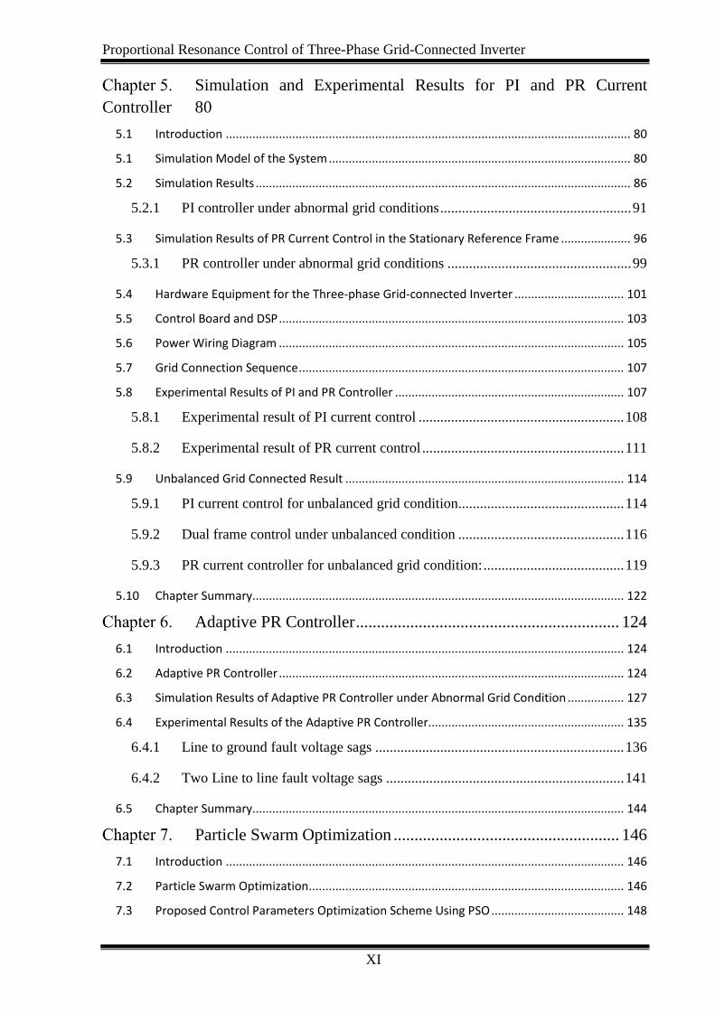
Simulation and Experimental Results for PI and PR Current
Controller 80
5.1 Introduction .......................................................................................................................... 80
5.1 Simulation Model of the System ........................................................................................... 80
5.2 Simulation Results ................................................................................................................. 86
5.2.1 PI controller under abnormal grid conditions ..................................................... 91
5.3 Simulation Results of PR Current Control in the Stationary Reference Frame ..................... 96
5.3.1 PR controller under abnormal grid conditions ................................................... 99
5.4 Hardware Equipment for the Three-phase Grid-connected Inverter ................................. 101
5.5 Control Board and DSP ........................................................................................................ 103
5.6 Power Wiring Diagram ........................................................................................................ 105
5.7 Grid Connection Sequence .................................................................................................. 107
5.8 Experimental Results of PI and PR Controller ..................................................................... 107
5.8.1 Experimental result of PI current control ......................................................... 108
5.8.2 Experimental result of PR current control ........................................................ 111
5.9 Unbalanced Grid Connected Result .................................................................................... 114
5.9.1 PI current control for unbalanced grid condition.............................................. 114
5.9.2 Dual frame control under unbalanced condition .............................................. 116
5.9.3 PR current controller for unbalanced grid condition: ....................................... 119
5.10 Chapter Summary................................................................................................................ 122
Adaptive PR Controller ............................................................... 124
6.1 Introduction ........................................................................................................................ 124
6.2 Adaptive PR Controller ........................................................................................................ 124
6.3 Simulation Results of Adaptive PR Controller under Abnormal Grid Condition ................. 127
6.4 Experimental Results of the Adaptive PR Controller........................................................... 135
6.4.1 Line to ground fault voltage sags ..................................................................... 136
6.4.2 Two Line to line fault voltage sags .................................................................. 141
6.5 Chapter Summary................................................................................................................ 144
Particle Swarm Optimization ...................................................... 146
7.1 Introduction ........................................................................................................................ 146
7.2 Particle Swarm Optimization ............................................................................................... 146
7.3 Proposed Control Parameters Optimization Scheme Using PSO ........................................ 148

Proportional Resonance Control of Three-Phase Grid-Connected Inverter
XII
7.4 Simulation Results of Using PSO Method ............................................................................ 151
7.4.1 Simulation Results of Using PSO under Unbalanced Grid Conditions ........... 154
7.5 Chapter Summary ................................................................................................................ 158
Conclusion and Future work ....................................................... 159
8.1 Introduction ......................................................................................................................... 159
8.2 Conclusion ........................................................................................................................... 159
8.3 Future Work ......................................................................................................................... 162
References ......................................................................................................... 164
Appendix A ....................................................................................................... 173
A.1 Introduction............................................................................................................................... 173
A.2 Clark and Park Transformation.................................................................................................. 173
A.3 LCL Filter Mathematical Model: ................................................................................................ 175
A.3 Current Control of Grid-connected Inverter ............................................................................. 176
Appendix B ........................................................................................................ 179
B.1 Introduction ............................................................................................................................... 179
B.2 Isolation and Varic Transformers .............................................................................................. 179
B.3 Three-phase Inverter ................................................................................................................. 181
B.4 Digital Signal Processor ............................................................................................................. 184
B.5 Analog-to-Digital Converter ...................................................................................................... 184
B.6 Current Sensor ........................................................................................................................... 184
B.8 Voltage Sensor ........................................................................................................................... 185
B.9 LabVIEW .................................................................................................................................... 185
B.10 Experimental Result RL Load ................................................................................................... 186
Appendix C ........................................................................................................ 188
C.1 Introduction ............................................................................................................................... 188
C.2 The Method of Decomposition of the Voltage .......................................................................... 188

Proportional Resonance Control of Three-Phase Grid-Connected Inverter
XIII
List of Tables
Table 3.1 Comparison of SVM and SPWM modulation techniques ........................................ 44
Table 3.2 The phase voltage levels for different switching states ............................................ 46
Table 5.1 Three-phase inverter simulation parameters ............................................................ 83
Table 5.2 PI controller parameters ........................................................................................... 86
Table 5.3 PR controller parameters .......................................................................................... 97
Table 5.4 Three phase inverter practical parameters .............................................................. 108
Table 6.1 Adaptive PR controller simulation parameters ...................................................... 127
Table 6.2 Adaptive PR controller practical parameters 𝑘𝑝, 𝑘𝑖 .............................................. 135
Table 7.1 Iteration numbers the control parameters ............................................................... 157

Chapter 1: Introduction
1
Table of Figures
Figure 1.1 PV capacity installed in the U.K ............................................................................... 6
Figure 1.2. Photovoltaic PV system at King Abdullah University (KAUST), Saudi Arabia [7]
.................................................................................................................................................... 7
Figure 1.3 Basic single line diagram of three-phase grid-connected PV inverter ...................... 8
Figure 1.4 Processing stages for single line diagram of the three-phase PV gird connected
inverter: (a) single-stage case (b) multi-stage case ................................................................... 10
Figure 1.5 Two-level three phase inverter (VSI) ...................................................................... 11
Figure 1.6 Filter configuration schemes: (a) L-filter; (b) LC-filter; (c) LCL-filter; (d) LCL-filter
with damping resistor ............................................................................................................... 12
Figure 1.7 Zero crossing detection method .............................................................................. 13
Figure 1.8 Basic PLL scheme ................................................................................................... 14
Figure 1.9 The PLL scheme in SRF ......................................................................................... 14
Figure 1.10 Basic virtual flux scheme ...................................................................................... 15
Figure 2.1 Basic single line diagram of the three-phase grid-connected inverter with current
control scheme .......................................................................................................................... 20
Figure 2.2 a) Positive sequence components , b) Negative sequence components .................. 27
Figure 2.3 The decoupled double synchronous reference frame PLL ...................................... 29
Figure 2.4 Delayed signal cancellation method....................................................................... 30
Figure 2.5 General structure of the PSO optimization algorithm ............................................. 36
Figure 3.1 Single line diagrams of three-phase grid-connected inverter: (a) single stage, (b)
double stage .............................................................................................................................. 38
Figure 3.2 Equivalent circuit I-V characteristics of the solar module ...................................... 38
Figure 3.3 I-V characteristic plot of the PV module ................................................................ 40
Figure 3.4 P-V characteristic plot of the PV module ............................................................... 40
Figure 3.5 The three-phase inverter .......................................................................................... 41
Figure 3.6 Sine-triangle modulation for the three-phase waveform with three switched
waveform legs: a, b and c ......................................................................................................... 43
Figure 3.7 Space vector hexagon .............................................................................................. 44
Figure 3.8 Reference voltage vector ......................................................................................... 46
Figure 3.9 Hysteresis band PWM control ................................................................................ 48
Figure 3.10 Third-harmonic injection waveform with carrier waveform ................................ 49

Chapter 1: Introduction
2
Figure 3.11 Single-phase equivalent circuit LCL filter ........................................................... 50
Figure 3.12 LCL filter Bode diagram ...................................................................................... 52
Figure 3.13 Equivalent circuit of single-phase LCL filter with damping resistor ................... 53
Figure 3.14 LCL filter with damping resistor .......................................................................... 54
Figure 4.1 The positive, negative and zero sequences system ................................................. 57
Figure 4.2 The symmetric components decomposition two-phase system .............................. 59
Figure 4.3 The bode plot of the low pass filter ........................................................................ 61
Figure 4.4 Block diagram of positive and negative decomposition ......................................... 63
Figure 4.5 single line diagram of three-phase grid-connected inverter with current control
scheme ...................................................................................................................................... 64
Figure 4.6 PI controller in synchronous reference scheme ...................................................... 65
Figure 4.7 PI control scheme in the time domain .................................................................... 66
Figure 4.8 PI controller Bode diagram..................................................................................... 68
Figure 4.9 Closed loop of an inverter with LCL filter using PI controller .............................. 70
Figure 4.10 Bode plot of the open loop system ....................................................................... 71
Figure 4.11 Root locus of the PI controller .............................................................................. 72
Figure 4.12 PR controller in the stationary reference frame control ....................................... 73
Figure 4.13 Control Diagram of PR controller implementation .............................................. 74
Figure 4.14 The Bode plots of ideal PR and non-ideal PR controller ..................................... 75
Figure 4.15 Closed loop of an inverter with LCL filter using PR controller ........................... 77
Figure 4.16 The bode blot of the open loop system ................................................................. 78
Figure 4.17 The root locus of the closed loop system ............................................................. 78
Figure 5.1 Simulink model of the three-phase grid-connected inverter .................................. 84
Figure 5.2 PLL, voltage and current transformations .............................................................. 85
Figure 5.3 The three-phase grid voltage .................................................................................. 86
Figure 5.4 The three-phase grid current ................................................................................... 87
Figure 5.5 Measured DC voltage ............................................................................................. 87
Figure 5.6 Measured PI controller for DC voltage .................................................................. 88
Figure 5.7 Reference and measured d-axis current ................................................................. 89
Figure 5.8 Reference and measured q-axis current .................................................................. 89
Figure 5.9 The step response of the reference and measured current 𝑖𝑑 ................................. 90
Figure 5.10 The active and reactive power waveform ............................................................. 90
Figure 5.11 The three-phase voltage waveform under balanced voltage sags and swell ........ 92
Figure 5.12 The three-phase current waveform under balanced voltage sags and swell ......... 92

Chapter 1: Introduction
3
Figure 5.13 The reference and measured d-axis current id for PI controller ............................ 93
Figure 5.14 The reference and measured iq for PI controller ................................................... 94
Figure 5.15 The FFT of the current waveform using PI controller .......................................... 94
Figure 5.16 The three-phase voltage under unbalanced conditions ......................................... 95
Figure 5.17 The three-phase distorted current waveform under unbalanced conditions.......... 95
Figure 5.18 The three-phase current waveform under unabalnced grid conditions using
decompestion method ............................................................................................................... 96
Figure 5.19 The reference and measured id for in the positive-sequence controller under
unabalnced grid conditions ....................................................................................................... 96
Figure 5.20 Measured phase voltage waveform ....................................................................... 97
Figure 5.21 Phase current waveform ........................................................................................ 97
Figure 5.22 The alpha current in the stationary reference frame.............................................. 98
Figure 5.23 The beta current in the stationary reference frame ................................................ 98
Figure 5.24 The three-phase grid voltage waveform under voltage sags ................................. 99
Figure 5.25 The three-phase current using PR controller ......................................................... 99
Figure 5.26 The alpha current waveform ................................................................................ 100
Figure 5.27 The beta current waveform ................................................................................. 100
Figure 5.28 The FFT of the current waveform using PR controller ....................................... 101
Figure 5.29 Three-phase inverter test rig................................................................................ 102
Figure 5.30 The three-phase inverter rig metal cage from inside ........................................... 102
Figure 5.31 Newcastle University control board .................................................................... 104
Figure 5.32 Screen shot of LabView ...................................................................................... 104
Figure 5.33 Power wiring diagram ......................................................................................... 106
Figure 5.34 Three-phase voltage waveform at PCC............................................................... 109
Figure 5.35 Three-phase current waveform using PI controller ............................................. 109
Figure 5.36 The reference and measured 𝑖𝑑 and 𝑖𝑞 ............................................................. 110
Figure 5.37 The reference and measured 𝑖𝑑 and 𝑖𝑞under step response ............................... 110
Figure 5.38 The three-phase current waveform with grid voltage using PR controller ......... 111
Figure 5.39 The reference and measured alpha and beta currents waveform ....................... 112
Figure 5.40 The current waveform with step response .......................................................... 112
Figure 5.41 The alpha reference and measured current waveform with response ................. 113
Figure 5.42 The THD of the current waveform of PR controller with HC ............................ 114
Figure 5.43 Three-phase unbalanced voltage ......................................................................... 115
Figure 5.44 Three-phase current waveform under unbalance condition ................................ 115

Chapter 1: Introduction
4
Figure 5.45 Three-phase current under unbalance condition with feed-forward voltage ..... 116
Figure 5.46 The reference and measured 𝑑𝑞 + and 𝑑𝑞 − .................................................... 117
Figure 5.47 The three-phase unbalanced voltage in phase a .................................................. 117
Figure 5.48 The three-phase current waveform ..................................................................... 118
Figure 5.49 The FFT of the current waveform using dual PI controller ................................ 118
Figure 5.50 The three-phase voltage with unbalanced line to line voltage sags. ................... 119
Figure 5.51 The three-phase current waveform. .................................................................... 119
Figure 5.52 Three-phase voltage with unbalance voltage sag ............................................... 120
Figure 5.53 The three-phase current waveform with unbalance voltage sag in phase a ........ 121
Figure 5.54 The reference and measured alpha and beta current using conventional PR
controller waveforms ............................................................................................................. 121
Figure 5.55 The FFT waveform of the current waveform ..................................................... 122
Figure 6.1 Flow chart of the proposed adaptive PR controller .............................................. 126
Figure 6.2 proposed adaptive PR controller structure............................................................ 126
Figure 6.3 Screenshot of the adaptive PR controller ............................................................ 128
Figure 6.4 The voltage waveform with 30% voltage sag ...................................................... 128
Figure 6.4 The current waveform with 30% voltage sag ....................................................... 129
Figure 6.5 The adaptive PR controller alpha current using medium gains ............................ 129
Figure 6.6 The beta current waveform for adaptive PR controller using medium gains ....... 130
Figure 6.7 The single phase-to-ground voltage sags .............................................................. 130
Figure 6.8 The three-phase current waveform under unbalanced voltage sags ..................... 131
Figure 6.9 The adaptive PR controller alpha current using medium gains ............................ 131
Figure 6.10 The beta current waveform for adaptive PR controller using medium gains ..... 132
Figure 6.10 The two-phase-to-ground voltage sag ................................................................ 133
Figure 6.11 The distorted current waveform under unbalanced line to line fault .................. 133
Figure 6.12 The three-phase current waveform under unbalanced conditions ...................... 134
Figure 6.14 The stationary reference frame alpha current ..................................................... 134
Figure 6.15 The stationary reference frame beta current ....................................................... 135
Figure 6.16 Three-phase voltage with unbalance voltage sag in phase a by 20% ................. 136
Figure 6.17 Three-phase current waveform using adaptive PR controller ............................ 137
Figure 6.18 The FFT of the current waveform ...................................................................... 137
Figure 6.16 Three-phase voltage with unbalance voltage sag in phase a by 30% ................. 138
Figure 6.17 The three-phase current waveform with unbalance voltage sag in phase a by using
medium adaptive controls gains ............................................................................................. 138

Chapter 1: Introduction
5
Figure 6.18 The FFT of the current waveform using medium adaptive controls gains ......... 139
Figure 6.19 The reference and measured alpha and beta current using medium gains of the
adaptive PR controller ............................................................................................................ 139
Figure 6.20 Three-phase voltage with 50% unbalance voltage sag in phase a using higher gains
for the adaptive PR control .................................................................................................... 140
Figure 6.21 The three-phase current waveform with 50% unbalance voltage sag in phase a 140
Figure 6.22 The FFT current waveform using higher adaptive controls gains ...................... 141
Figure 6.23 The unbalanced three-phase voltage with line to line voltage sags .................... 141
Figure 6.24 The three-phase current waveform with line to line voltage sags using low control
gains ........................................................................................................................................ 142
Figure 6.25 The reference and measured alpha and beta current using medium gains of the
adaptive PR controller ............................................................................................................ 143
Figure 6.26 The reference and measured alpha and beta current with step response............. 143
Figure 6.27 The FFT of the current waveform two line-to-line faults ................................... 144
Figure 7.1 Particle Swarm Optimisation flowchart (PSO) ..................................................... 148
Figure 7.2 PSO optimization in the synchronous reference frame ......................................... 149
Figure 7.3 Optimization in the stationary reference frame using PR controller.................... 150
Figure 7.4 General structure of the PSO optimization algorithm ........................................... 151
Figure 7.5 The three-phase voltage waveform using PSO ..................................................... 152
Figure 7.6 The three-phase current waveform Using PSO ..................................................... 152
Figure 7.7 The reference and measured id current using PSO ................................................ 153
Figure 7.8 The reference and measured iq current using PSO ................................................ 153
Figure 7.9 The reference and measured i-alpha using PSO .................................................... 154
Figure 7.10 The reference and measured i-beta using PSO .................................................... 154
Figure 7.11 The unbalanced voltage waveform ..................................................................... 155
Figure 7.12 The three-phase current waveform...................................................................... 155
Figure 7.13 The reference and measured i_alpha under unbalance condition ...................... 156
Figure 7.14 The reference and measured i_beta under unbalance condition ........................ 156
Figure 7.15 The error convergence curve ............................................................................... 157
Figure 7.16 The FFT of the phase current waveform using PSO ........................................... 158

Chapter 1: Introduction
6
Introduction
1.1 Background and Motivation
The aggressive use of non–renewable resources has caused major issues such as the production
of more pollution and greenhouse gas emissions leading to environmental concerns [1].
Furthermore, the upsurge seen in global energy demand from fossil fuel suppliers has resulted
in higher oil prices [2]. These issues have encouraged organizations to use renewable sources
instead of non-renewable energy sources. In the last few years, distributed power generation
(DGs) based on renewable energy has continued to develop across the world due to its benefits
for the global environment.
Photovoltaic (PV) energy is a renewable energy that can be identified as a rapidly growing
element of renewable energy existing in the market, and according to renewable energy policy
network for the 21st century (REN21) to be the biggest supplier of renewable energy [3].
Statistics from the European Photovoltaic Industry Association (EPIA) have shown that in 2014
there was 40 GW installed globally. In Europe, there was 75% increase in installed PV system
reaching a capacity of 21.9 GW. U.K leading the way and has installed PV capacity 5.4 GW in
2014 from 0.96 GW in 2010 as shown in Figure 1.1[4]. Overall, global PV capacity had
increased to 177 GW by end of 2014 [5].
Figure 1.1 PV capacity installed in the U. K

Chapter 1: Introduction
7
Saudi Arabia is one of the developing countries that is leading producers of PV systems in the
Middle East. Figure 1.2 shows the 2 MW grid–connected PV system at the King Abdullah
University for Science and Technology (KAUST) [6], and this system can reduce annual carbon
emissions in the region by 1700 tons.
Figure 1.2. Photovoltaic PV system at KAUST, Saudi Arabia [7]
The price of PV panels is one of the main issues which discourages consumers from adopting
these systems. Therefore, improvements in PV technology are ongoing and, in the days to
come, its cost will drop substantially, something identified as attributable to the solar cells
effectiveness and the size of the cells. Consequently, per unit capacity has been improved [8].
Hence, the cost of PV panel production continues to decrease, and solar power generation will
become comparable to other forms of renewable energy [9].
Distributed generators can generate electricity at or near the customer place where it is used as
different to the normal mode of power generation. The utilization of power electronic
technology in power system applications has been steadily increasing during recent decades.
The continuous improvement of semiconductor device technology and the availability of digital
control systems with endlessly increasing performance have reinforced this development.
Power electronic converter technology has also been an important enabling factor for recent
developments in distributed generation and renewable energy systems, including photovoltaic
systems due to several advantages and factors. A smaller size and lighter weight are important
factors which have led manufacturers to produce smaller power electronic converter products
for businesses customers. In addition, this high conversion efficiency and the capability to
Chapter 1: Introduction
8
control the power from a source to the utility load play an important role in the growth of power
electronic systems. As a result, such systems can be found in many applications of different
kinds for energy conversion, uninterruptible power supply (UPS), transportation, switch mode
power supply, utility systems, aerospace, telecommunications, factory automation, process
control and many other fields.
In recent years, voltage source converters (VSCs) have been increasingly developed supported
by this widespread with many benefits in industrial application. VSCs can be used in adjustable
speed electric drive systems [10] and UPS applications [11, 12]. VSCs, which are operating as
active rectifiers, has recently been seen as increasingly pertinent options to replace diode
rectifiers or line-commutated converters. This is owing to the pulse width modulated (PWM)
operation, that enables imperfect current distortion and concentrated harmonic filter necessities
composed to allow control of the power factor and DC-link voltage [13, 14]. Moreover, VSCs
are further used for distributed energy resources like photovoltaic and fuel cell systems, all of
which innately deliver a direct current (DC) output and are contingent on power from sunlight
and store it via solar cells using either batteries or any other generation electronic converters
for incorporation within the AC grid [15, 16]. Solar panels can extract electrical energy to feed
distribution farms or utility grids. Typically, PV panels are interfaced with utility grid via a
power electronic converter. Pulse width modulation (PWM) techniques are used to control the
three-phase power converter. In order to connect the PV module to the utility grid, a three-phase
inverter is used.
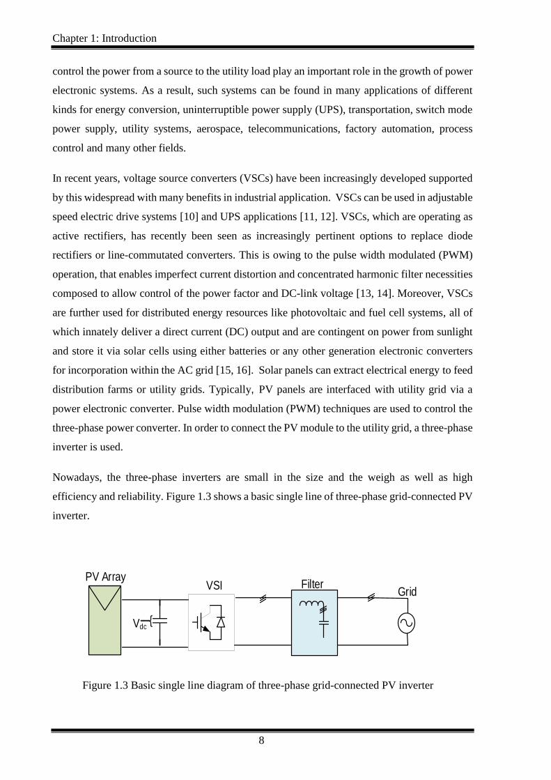
Nowadays, the three-phase inverters are small in the size and the weigh as well as high
efficiency and reliability. Figure 1.3 shows a basic single line of three-phase grid-connected PV
inverter.
Vdc
PV Array VSI
GridFilter
Figure 1.3 Basic single line diagram of three-phase grid-connected PV inverter
Chapter 1: Introduction
9
On the other hand, in connecting the converters to the utility grid there are international
recommendations that must be observed. These recommendations could vary from country to
country, and some of the criteria follow [17, 18]:
DC current level injected.
Total harmonic distortion (THD).
The grounding of the system.
Voltage, current, and frequency.
Automatic reconnection and synchronization.
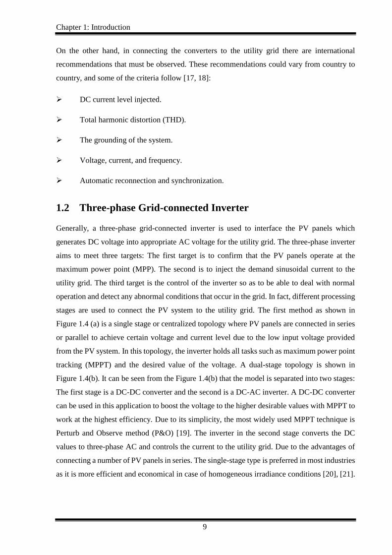
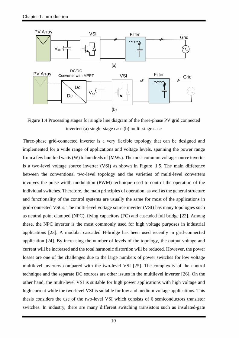
1.2 Three-phase Grid-connected Inverter
Generally, a three-phase grid-connected inverter is used to interface the PV panels which
generates DC voltage into appropriate AC voltage for the utility grid. The three-phase inverter
aims to meet three targets: The first target is to confirm that the PV panels operate at the
maximum power point (MPP). The second is to inject the demand sinusoidal current to the
utility grid. The third target is the control of the inverter so as to be able to deal with normal
operation and detect any abnormal conditions that occur in the grid. In fact, different processing
stages are used to connect the PV system to the utility grid. The first method as shown in
Figure 1.4 (a) is a single stage or centralized topology where PV panels are connected in series
or parallel to achieve certain voltage and current level due to the low input voltage provided
from the PV system. In this topology, the inverter holds all tasks such as maximum power point
tracking (MPPT) and the desired value of the voltage. A dual-stage topology is shown in
Figure 1.4(b). It can be seen from the Figure 1.4(b) that the model is separated into two stages:
The first stage is a DC-DC converter and the second is a DC-AC inverter. A DC-DC converter
can be used in this application to boost the voltage to the higher desirable values with MPPT to
work at the highest efficiency. Due to its simplicity, the most widely used MPPT technique is
Perturb and Observe method (P&O) [19]. The inverter in the second stage converts the DC
values to three-phase AC and controls the current to the utility grid. Due to the advantages of
connecting a number of PV panels in series. The single-stage type is preferred in most industries
as it is more efficient and economical in case of homogeneous irradiance conditions [20], [21].
Chapter 1: Introduction
10
Vdc
PV Array
GridFilter VSI
(a)
(b)
Vdc
VSIDC/DC
Converter with MPPT
Dc
Dc
GridFilterPV Array
Figure 1.4 Processing stages for single line diagram of the three-phase PV grid connected
inverter: (a) single-stage case (b) multi-stage case
Three-phase grid-connected inverter is a very flexible topology that can be designed and
implemented for a wide range of applications and voltage levels, spanning the power range
from a few hundred watts (W) to hundreds of (MWs). The most common voltage source inverter
is a two-level voltage source inverter (VSI) as shown in Figure 1.5. The main difference
between the conventional two-level topology and the varieties of multi-level converters
involves the pulse width modulation (PWM) technique used to control the operation of the
individual switches. Therefore, the main principles of operation, as well as the general structure
and functionality of the control systems are usually the same for most of the applications in
grid-connected VSCs. The multi-level voltage source inverter (VSI) has many topologies such
as neutral point clamped (NPC), flying capacitors (FC) and cascaded full bridge [22]. Among
these, the NPC inverter is the most commonly used for high voltage purposes in industrial
applications [23]. A modular cascaded H-bridge has been used recently in grid-connected
application [24]. By increasing the number of levels of the topology, the output voltage and
current will be increased and the total harmonic distortion will be reduced. However, the power
losses are one of the challenges due to the large numbers of power switches for low voltage
multilevel inverters compared with the two-level VSI [25]. The complexity of the control
technique and the separate DC sources are other issues in the multilevel inverter [26]. On the
other hand, the multi-level VSI is suitable for high power applications with high voltage and
high current while the two-level VSI is suitable for low and medium voltage applications. This
thesis considers the use of the two-level VSI which consists of 6 semiconductors transistor
switches. In industry, there are many different switching transistors such as insulated-gate
Chapter 1: Introduction
11
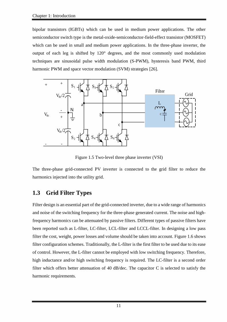
bipolar transistors (IGBTs) which can be used in medium power applications. The other
semiconductor switch type is the metal-oxide-semiconductor-field-effect transistor (MOSFET)
which can be used in small and medium power applications. In the three-phase inverter, the
output of each leg is shifted by 120° degrees, and the most commonly used modulation
techniques are sinusoidal pulse width modulation (S-PWM), hysteresis band PWM, third
harmonic PWM and space vector modulation (SVM) strategies [26].
- -
+
Vdc
Grid
a
b
c
+
+
-
Vdc/2
Vdc/2
N
S1
S2
S3
S4
S5
S6
L
C
Filter
Figure 1.5 Two-level three phase inverter (VSI)
The three-phase grid-connected PV inverter is connected to the grid filter to reduce the
harmonics injected into the utility grid.
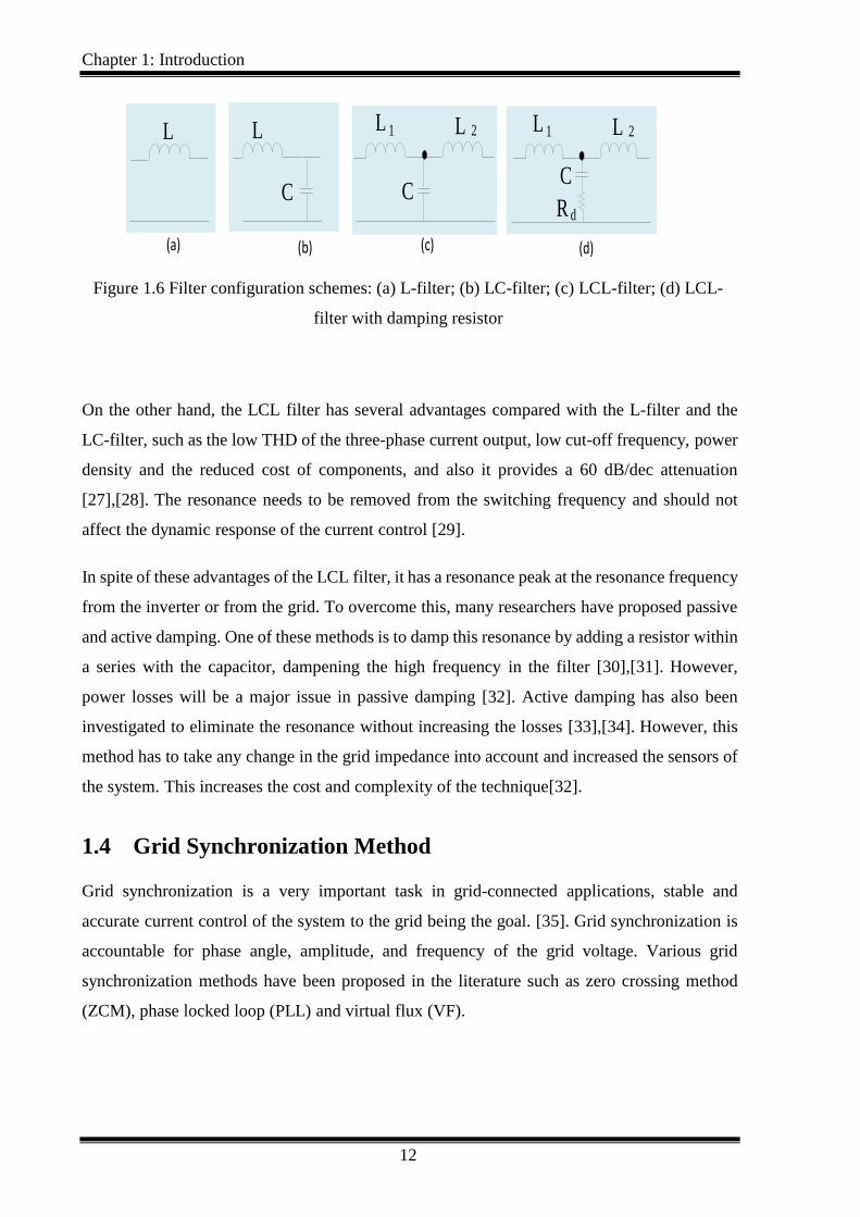
1.3 Grid Filter Types
Filter design is an essential part of the grid-connected inverter, due to a wide range of harmonics
and noise of the switching frequency for the three-phase generated current. The noise and high-
frequency harmonics can be attenuated by passive filters. Different types of passive filters have
been reported such as L-filter, LC-filter, LCL-filter and LCCL-filter. In designing a low pass
filter the cost, weight, power losses and volume should be taken into account. Figure 1.6 shows
filter configuration schemes. Traditionally, the L-filter is the first filter to be used due to its ease
of control. However, the L-filter cannot be employed with low switching frequency. Therefore,
high inductance and/or high switching frequency is required. The LC-filter is a second order
filter which offers better attenuation of 40 dB/dec. The capacitor C is selected to satisfy the
harmonic requirements.
Chapter 1: Introduction
12
L 1 L 2
C
L
C
(b)(a)
L L 1 L 2
C
dR
(d)(c)
Figure 1.6 Filter configuration schemes: (a) L-filter; (b) LC-filter; (c) LCL-filter; (d) LCL-
filter with damping resistor
On the other hand, the LCL filter has several advantages compared with the L-filter and the
LC-filter, such as the low THD of the three-phase current output, low cut-off frequency, power
density and the reduced cost of components, and also it provides a 60 dB/dec attenuation
[27],[28]. The resonance needs to be removed from the switching frequency and should not
affect the dynamic response of the current control [29].
In spite of these advantages of the LCL filter, it has a resonance peak at the resonance frequency
from the inverter or from the grid. To overcome this, many researchers have proposed passive
and active damping. One of these methods is to damp this resonance by adding a resistor within
a series with the capacitor, dampening the high frequency in the filter [30],[31]. However,
power losses will be a major issue in passive damping [32]. Active damping has also been
investigated to eliminate the resonance without increasing the losses [33],[34]. However, this
method has to take any change in the grid impedance into account and increased the sensors of
the system. This increases the cost and complexity of the technique[32].
1.4 Grid Synchronization Method
Grid synchronization is a very important task in grid-connected applications, stable and
accurate current control of the system to the grid being the goal. [35]. Grid synchronization is
accountable for phase angle, amplitude, and frequency of the grid voltage. Various grid
synchronization methods have been proposed in the literature such as zero crossing method
(ZCM), phase locked loop (PLL) and virtual flux (VF).
Chapter 1: Introduction
13
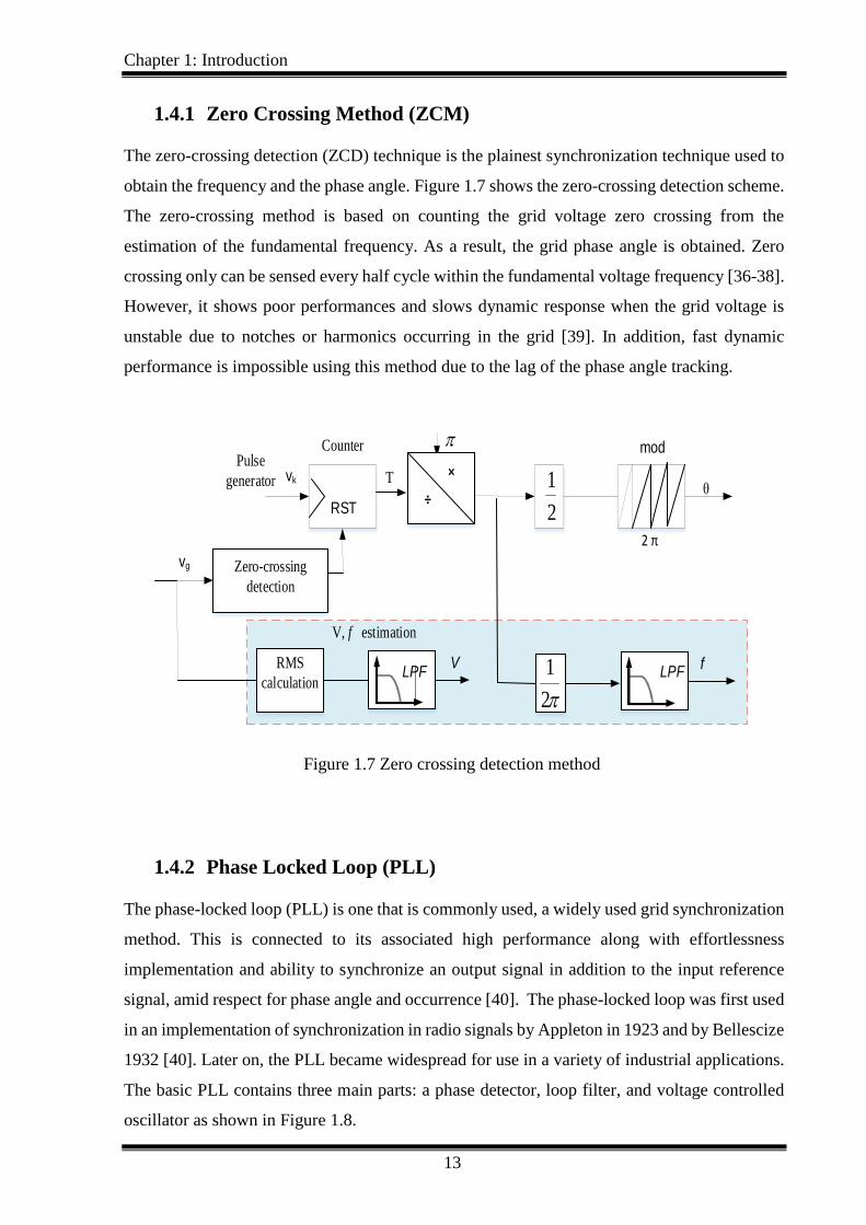
1.4.1 Zero Crossing Method (ZCM)
The zero-crossing detection (ZCD) technique is the plainest synchronization technique used to
obtain the frequency and the phase angle. Figure 1.7 shows the zero-crossing detection scheme.
The zero-crossing method is based on counting the grid voltage zero crossing from the
estimation of the fundamental frequency. As a result, the grid phase angle is obtained. Zero
crossing only can be sensed every half cycle within the fundamental voltage frequency [36-38].
However, it shows poor performances and slows dynamic response when the grid voltage is
unstable due to notches or harmonics occurring in the grid [39]. In addition, fast dynamic
performance is impossible using this method due to the lag of the phase angle tracking.
modCounter
θ
2 π
RST
2
1
2
1×
÷
T
Zero-crossing
detection
V fRMS
calculation
vk
V, f estimation
LPF
vg
Pulse
generator
LPF
Figure 1.7 Zero crossing detection method
1.4.2 Phase Locked Loop (PLL)
The phase-locked loop (PLL) is one that is commonly used, a widely used grid synchronization
method. This is connected to its associated high performance along with effortlessness
implementation and ability to synchronize an output signal in addition to the input reference
signal, amid respect for phase angle and occurrence [40]. The phase-locked loop was first used
in an implementation of synchronization in radio signals by Appleton in 1923 and by Bellescize
1932 [40]. Later on, the PLL became widespread for use in a variety of industrial applications.
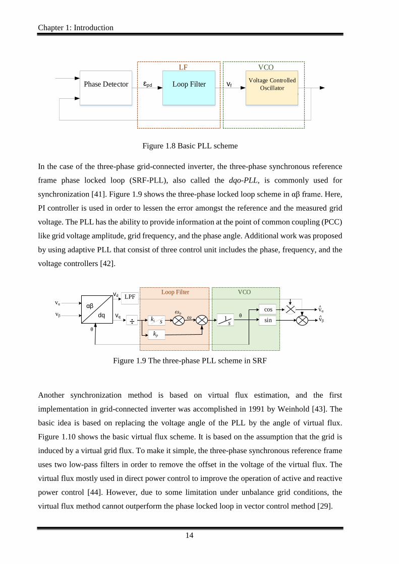
The basic PLL contains three main parts: a phase detector, loop filter, and voltage controlled
oscillator as shown in Figure 1.8.
Chapter 1: Introduction
14
θ
Voltage Controlled
OscillatorLoop Filter Phase Detector ɛpd vf
LF VCO
Figure 1.8 Basic PLL scheme
In the case of the three-phase grid-connected inverter, the three-phase synchronous reference
frame phase locked loop (SRF-PLL), also called the dqo-PLL, is commonly used for
synchronization [41]. Figure 1.9 shows the three-phase locked loop scheme in αβ frame. Here,
PI controller is used in order to lessen the error amongst the reference and the measured grid
voltage. The PLL has the ability to provide information at the point of common coupling (PCC)
like grid voltage amplitude, grid frequency, and the phase angle. Additional work was proposed
by using adaptive PLL that consist of three control unit includes the phase, frequency, and the
voltage controllers [42].
1
LPF
sin÷
αβ
dqcos
ski
kp
ωoω
s
vα
vβ
vd
vq
vα
vβ
Loop Filter
˄
˄ θ
θ
VCO
Figure 1.9 The three-phase PLL scheme in SRF
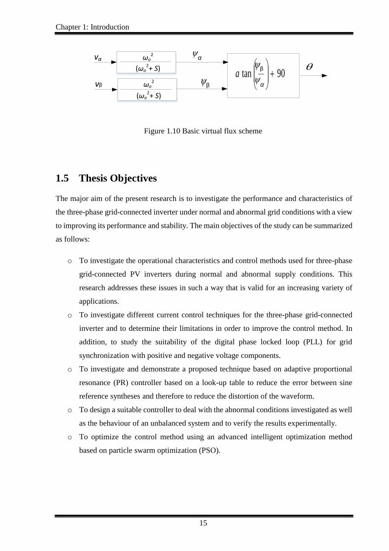
Another synchronization method is based on virtual flux estimation, and the first
implementation in grid-connected inverter was accomplished in 1991 by Weinhold [43]. The
basic idea is based on replacing the voltage angle of the PLL by the angle of virtual flux.
Figure 1.10 shows the basic virtual flux scheme. It is based on the assumption that the grid is
induced by a virtual grid flux. To make it simple, the three-phase synchronous reference frame
uses two low-pass filters in order to remove the offset in the voltage of the virtual flux. The
virtual flux mostly used in direct power control to improve the operation of active and reactive
power control [44]. However, due to some limitation under unbalance grid conditions, the
virtual flux method cannot outperform the phase locked loop in vector control method [29].
Chapter 1: Introduction
15
90tan
a
ωo
2
(ωo2+ S)
ωo2
(ωo2+ S)
vα
β
α
vβ
β
α
Figure 1.10 Basic virtual flux scheme
1.5 Thesis Objectives
The major aim of the present research is to investigate the performance and characteristics of
the three-phase grid-connected inverter under normal and abnormal grid conditions with a view
to improving its performance and stability. The main objectives of the study can be summarized
as follows:
o To investigate the operational characteristics and control methods used for three-phase
grid-connected PV inverters during normal and abnormal supply conditions. This
research addresses these issues in such a way that is valid for an increasing variety of
applications.
o To investigate different current control techniques for the three-phase grid-connected
inverter and to determine their limitations in order to improve the control method. In
addition, to study the suitability of the digital phase locked loop (PLL) for grid
synchronization with positive and negative voltage components.
o To investigate and demonstrate a proposed technique based on adaptive proportional
resonance (PR) controller based on a look-up table to reduce the error between sine
reference syntheses and therefore to reduce the distortion of the waveform.
o To design a suitable controller to deal with the abnormal conditions investigated as well
as the behaviour of an unbalanced system and to verify the results experimentally.
o To optimize the control method using an advanced intelligent optimization method
based on particle swarm optimization (PSO).
Chapter 1: Introduction
16
1.6 Contributions of the Thesis
This research presented in this thesis the performance of the three-phase grid-connected
inverter and takes into account the principles design, analysis and comparison of the current
control based on the PR controller in the stationary reference frame and PI controller in
synchronous reference frame for injected the current under abnormal conditions under any
circumstance such as grid fault, where the grid current varies from normal operating case.
Thus, the current control techniques based on the most suitable strategies that could achieve
better results during normal and abnormal conditions in the thesis are: positive and negative
sequence control (PNSC) and balance positive sequence control (BPSC).
Under abnormal grid conditions, the controlled signal instigating an unexpected decline in
voltage could promote a rise in the error between the reference signal, and the controlled
signal. This can be identified as creating large-scale aberration from its nominal value. The
implementation of the established PR controller cannot match the rise in error, in turn, this
lessens controller performance weakening. To get beyond this concern, this shows an
enhancement in present-day control using a novel adaptive PR controller. A novel method
for adaptive PR controller for abnormal conditions in the grid using a look-up table. The
adaptive PR control techniques have been used in the stationary reference frame to control
the current. The proposed control technique is qualified to provide low total harmonic
distortion (THD) in the inserted current even during the incidence of abnormal grid
conditions. The adaptive control has the ability to reduce the error.
Despite the fact that both PI and PR controllers are relatively straightforward to tune, and
are sometimes capable of dealing with many time-varying conditions, most disturbances
associated with grid-connected inverter technology, such as (grid voltage dip or changes in
network impedance) are significantly more challenging and depends on the designer to
obtain the best performance. This research also presented a novel concept of self-tuning of
the current controller using particle swarm optimization (PSO). An adaptive controller
tuned using PSO is presented to optimize the parameters of both PI and PR controllers for
the three-phase grid-connected inverter. There are many advantages of using PSO, such as
no additional hardware being required. Thus, it can be extended to other applications and
control methods. In addition, the proposed method is a self-tuning method and can thus be
suitable for industrial applications where manual tuning is not recommended for time and
Chapter 1: Introduction
17
cost reasons. Both the PI current control in the synchronous reference frame and the PR
current control in the stationary reference frame are considered in this study.
1.7 Publication
Publications from this work are listed below.
1. A. Althobaiti, M. Armstrong, and M. Elgendy. "Three-Phase, Grid-Connected Inverter
Using Different Control Schemes." Proceedings of the Eighth Saudi Students
Conference in the UK. 2016. [45].
2. A. Althobaiti, M. Armstrong, and M. A. Elgendy. "Current control of three-phase grid-
connected PV inverters using adaptive PR controller." Renewable Energy Congress
(IREC), 2016 7th International. IEEE, 2016.
3. A. Althobaiti, M. Armstrong and M. A. Elgendy, "Control parameters optimization of
a three-phase grid-connected inverter using particle swarm optimisation," 8th IET
International Conference on Power Electronics, Machines and Drives (PEMD 2016),
Glasgow, 2016.
4. Althobaiti, M. Armstrong, M. A. Elgendy and F. Mulolani, "Three-phase grid connected
PV inverters using the proportional resonance controller," 2016 IEEE 16th
International Conference on Environment and Electrical Engineering (EEEIC),
Florence, 2016.
5. A. Althobaiti, M. Armstrong and M. A. Elgendy, "Space vector modulation current
control of a three-phase PV grid-connected inverter," 2016 Saudi Arabia Smart
Grid(SASG), Jeddah, 2016, 1-6. 2016.
1.8 Thesis Outline:
The content of this thesis is described below:
Chapter 1: This chapter gives an introduction to the thesis, provides the background of
the grid-connected inverter, describes some of the more important points in research on
power electronics and emphasises the motivation and importance of the present research
work. This chapter also discusses the grid synchronization methods. In addition, the
present study’s aim and objectives, followed by thesis contributions and the publications
resulting from this research are presented.
Chapter 1: Introduction
18
Chapter 2: A literature review of various types of control methods for grid-connected
inverters is provided in this chapter describing the background and various types of
control and how their use affects the environment. Also, the challenges faced in the
development of these systems are highlighted here.
Chapter 3: This chapter considers the modelling and design of the three-phase grid-
connected inverter and grid synchronization in three-phase inverters under abnormal
conditions.
Chapter 4: Highlights the steps in the control approaches used for grid-connected
inverters in the synchronous rotating reference frame and stationary reference frame
Chapter 5: Simulations and practical results of the PI controller and PR controller are
presented. In addition, it presents experimental hardware equipment with an overview
of the hardware
Chapter 6: Simulation and practical results of adaptive PR controller are presented in
balance and unbalanced grid conditions. The controller has been tested with different
grid faults such as line-to-line fault and two line-to-line faults.
Chapter 7: This chapter present advanced optimization control method using Particle
Swarm Optimisation (PSO) to find the optimal control parameters of PI and PR
controller. Simulation results of the PI controller and PR controller are presented under
abnormal grid conditions.
Chapter 8: A summary of the research is provided in this chapter along with the
conclusions of the study. Possible future research work is then discusse.
Chapter 2: Literature Review
19
Literature Review
2.1 Introduction
The rapid increase in the use of distributed power generation systems (DPGS) grounded on
renewable energy sources has boosted the implementation of voltage source converters (VSCs)
in distribution networks. As a result, the voltage source inverter (VSI) and its control system
have become main elements of distributed generation. There has been an intense research effort
in the development and analysis of various current control techniques for the three-phase
applications during the last couple of decades. In addition, different methods of grid
synchronization have been proposed and analysed. Many studies have aimed to improve and
develop the control technique used firstly for electrical machine drive systems such doubly fed
induction generator (DFIG) also known as wound rotor induction generator. These techniques
are also successfully applied in grid-connected inverters and bidirectional AC-DC flywheel
converters to interface between the DPGS and the power grid. Moreover, active-reactive
voltage source converters have also become an interesting alternative for diode rectifiers or line
commuted converters due to pulse width modulation (PWM) technique. This method has the
ability to control the power factor and DC-link voltage which ensures a reduction in harmonics
of the system [46, 47].
The performance of a three-phase grid-connected inverter depends mainly on the quality of
current control to the load or the grid. This factor plays an important role in power electronics
in meeting the requirements of standards such as IEEE 519 and 1547 which require a maximum
of 5% for the current total harmonic distortion (THD) [48, 49]. In order to comply with the
above requirements, the three-phase grid-connected inverter should have very good current
control which has a good harmonic rejection.
The thesis focuses on the current controls techniques which depend on the voltage oriental
control.
2.2 Methods of Three-phase Current Control
In three-phase grid-connected inverter, current control is a high-status issue, which needs to be
dealt with. The main function of current control is to ensure that the reference signal is followed
Chapter 2: Literature Review
20
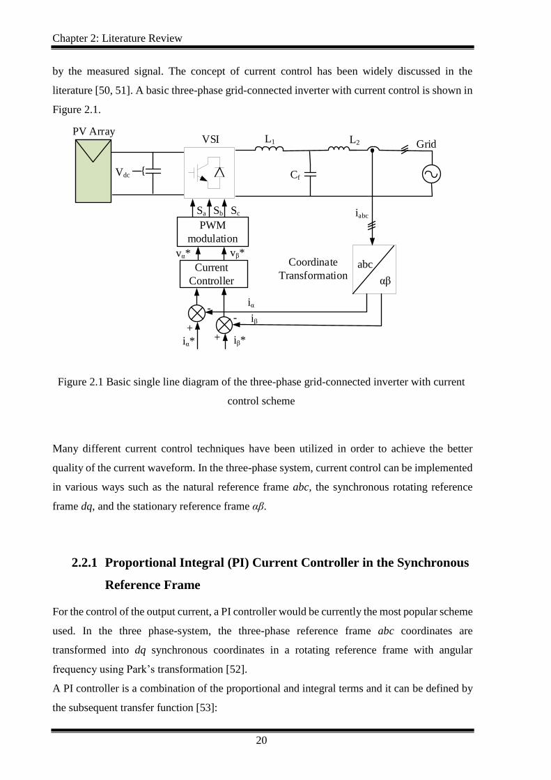
by the measured signal. The concept of current control has been widely discussed in the
literature [50, 51]. A basic three-phase grid-connected inverter with current control is shown in
Figure 2.1.
PWM
modulation
Sa Sb Sc
abc
Vdc
αβ
iabc
PV ArrayVSI L1
vα* vβ*
Cf
L2
iβ*iα*
Current
Controller
++
--
iα
iβ
Grid
Coordinate
Transformation
Figure 2.1 Basic single line diagram of the three-phase grid-connected inverter with current
control scheme
Many different current control techniques have been utilized in order to achieve the better
quality of the current waveform. In the three-phase system, current control can be implemented
in various ways such as the natural reference frame abc, the synchronous rotating reference
frame dq, and the stationary reference frame αβ.
2.2.1 Proportional Integral (PI) Current Controller in the Synchronous
Reference Frame
For the control of the output current, a PI controller would be currently the most popular scheme
used. In the three phase-system, the three-phase reference frame abc coordinates are
transformed into dq synchronous coordinates in a rotating reference frame with angular
frequency using Park’s transformation [52].
A PI controller is a combination of the proportional and integral terms and it can be defined by
the subsequent transfer function [53]:
Chapter 2: Literature Review
21
𝐺𝑝𝑖(𝑠) = 𝑘𝑝 +𝑘𝑖
𝑠 (2.1)
where 𝑘𝑝 is the proportional gain, 𝑘𝑖 is the integral gain of the PI controller.
The two current components in the rotating synchronous reference frame dq coordinates appear
as DC components. The d coordinate represents the direct component while q coordinate
represents the quadrature component. The PI current controller has a number of plus points, a
principal one being that it is relatively straightforward to use within the control system. This
makes it more preferable for engineering, and therefore control and filtering can be obtained.
However, the PI controller has the following drawbacks such as:
In a single-phase inverter, the PI controller has a steady state error in the stationary
reference frame which cannot be eliminated. This error is between the sinusoidal
reference signal and the output measured signal [54, 55].
PI controller has poor performance due to cross-coupling between d and q coordinators.
As a consequence, the functioning of the PI controller can be enriched by presenting a
decoupling term between the d and q coordinators and the voltage feedforward [30, 38,
56]
The PI controller is poor at eliminating the low order harmonics, and this can cause
problems when used in grid-connected applications [39].
The PI current controller requires more transformation from three to two phases, which
therefore requires more space in a low-cost fixed-point DSP [30].
To overcome these issues, many improvements have been implemented in PI
controllers. As a result, the feedforward control method is able to reduce the grid current
harmonics caused by grid voltage distortion without changing the dynamic response
[39].
2.2.2 Proportional Resonance (PR) Current Controller in Stationary
Reference Frame
Given the shortcomings of the PI controller, an alternative solution for a current controller has
been presented which is the proportional resonant controller (PR). The PR controller is a
combination of a proportional term and a resonant term. The PR controller has been used in the
stationary reference frame method [39], [57, 58]. Within the control system; grid current is

Chapter 2: Literature Review
22
conveyed to the stationary reference frame using Clark’s transformation from three-phase 𝑖𝑎,𝑏 ,𝑐
to 𝑖𝛼,𝛽 coordinators [59]. Hence, PR controller variables are sinusoidal. In addition, a PR
controller has several advantages which are as follows:
It has the capability to eradicate steady-state error by offering extra gain at the
particular resonant frequency of the controlled signal [60].
The PR controller has the capability to implement harmonic compensator (HC)
minus the introduction of any deviations in dynamic control; thus, this accomplishes
a high-quality current [61].
The intricacy of current control can be seen to be lower in a statutory reference frame
in comparison to the synchronous reference frame dq because Park’s transformation
does not need to be used in the control system.
Currents in α-β coordinates are not cross-coupled and so do not need to be decoupled
[62].
PR control can be used as a notch filter to compensate the harmonic in the control
signal [56].
The transfer function of the PR controller is given by:
𝐺𝑃𝑅(s) = 𝐾𝑝 + 𝐾𝑖
𝑠
(𝑠2 + 𝜔02)
(2.2)
Where, kp is the proportional gain, ki is the integral gain of the controller, 𝜔0 is the resonance
frequency.
To sidestep the problem of obtaining infinite gain at the resonant frequency; a non-ideal PR
controller can instead be used by including a bandwidth of the controller system. Although this
type of control provides very low steady-state tracking error, any such error will affect the
current control.
𝐺𝑃𝑅(s) = 𝐾𝑝 + 𝐾𝑖
2𝜔𝑐𝑠
(𝑠2 + 2𝜔𝑐𝑠+ω02)
(2.3)
where, kp is the proportional gain, ki is the integral gain of the controller, 𝜔0 is the resonance
frequency, and 𝜔𝑐 is the cut off frequency.
In grid-connected uses, it is useful to apply Harmonic Compensator (HC) terminologies in
parallel with the PR controller to focus upon low order harmonics (5th, 7th); these will be noted
as being problematic.

Chapter 2: Literature Review
23
The equation next is important for implementation of the HC:
𝐺𝐻𝐶(𝑠) = ∑2 𝐾𝑖ℎ 𝑠
𝑠2 + (ωh)2
ℎ=5,7
(2.4)
2.2.3 The abc Reference Frame Current Control
The first current control technique proposed for pulse width modulation (PWM) was based on
the three-phase reference frame [50], [63]. The principle of the control task is to keep the three-
phase measured current aligned with the three-phase reference current based on the state of
inverter switches. Therefore, the control depends on the output of the three-phase current of the
inverter compared with the phase current reference. One of the most common control
techniques using this reference frame is the hysteresis controller (HC) method. Hence, the
results of the three-phase errors are used at the same time to feed the PWM through the upper
and lower hysteresis bands in the loop. The advantages of this type of control are that it is easy
to implement in the three-phase system, and gives faster transit responses. However, the
aforementioned control has several drawbacks:
High switching frequency and high ripples are produced by the hysteresis bandwidth
[64].
There is interference between the phase currents which could lead to increased
distortion.
This controller has no fixed switching frequency, and therefore it has bad harmonic
performance and this leads the system to be unstable.
The abc reference frame parameters are independent of each other and therefore it is
necessary to generate the duty cycle for the PWM which will make the control technique
is more complex [65].
The abc reference frame could be used in synchronous reference frame using a PI
controller. However, due to the off-diagonal terms repressing the cross coupling
between the phases in the matrix which make the control technique is more
challengeable [39].
2.2.4 Other Control Strategy
Many recent methods have not used the vector orientated control approach. Direct power
control (DPC) is another control strategy based on active power and reactive power control [66,
67]. The advantages of this control technique are that it is a simple method and there is no need
for the internal control loop for the current or the voltage. However, high frequency is needed
Chapter 2: Literature Review
24
to obtain good performance. In addition, switching frequency is variable due to the use of
hysteresis comparators, which makes it difficult to design the grid filter [44].
On the other hand, other studies have used predictive control. This technique predicts the error
vector of the current waveform at the sampling modulation period [51, 68]. The concept of
predictive control has been used for direct power control by minimizing the error for active and
reactive power [69]. However, this method has issues in the grid filter which is affected by
unwanted frequencies due to the current spectrum distribution [70].
2.3 Power Quality
The three-phase grid-connected inverter is most commonly a factor in injection and absorption
of the power to the grid. An example of this would motor drives which concentrate absorbing
active power taken from the grid in order to reach the optimum performance of an electrical
motor. In normal grid conditions, the three-phase inverter injects all active power to the grid.
However, the widespread use of electronic-based loads and nonlinear loads has led to negative
effects on the power quality which is an important issue. Therefore, the term power quality can
be used to refer to any issues arising from an unusual situation in the system. The power quality
is commonly affected negatively when the system is subjected to abnormal conditions in the
voltage, current, and frequency when disturbances in the utility grid occur [71].
When operated in grid-connected applications, the three-phase grid-connected inverter can be
exposed to the disturbances, transients, and interruptions that propagate through the electric
power system. Thus, a large share of such disturbances and transients are likely to introduce
temporary unbalanced grid voltage conditions [72, 73]. Moreover, due to a low quality of DGs,
there are many causes for unbalanced voltage produced by a nonlinear load. Single phase
generators, unbalanced loads and the negative impact of induction motors [74],[75]. Therefore,
voltage disturbance in the grid has a negative effect on the grid and can cause a major trip and
high cost in general [76]. These abnormal conditions can be caused in the utility grid by short
circuit faults like a line to ground fault, voltage sags, voltage swell and injected harmonics.
These faults can be produced by abnormal situations in the grid such as direct on-line starting
of large motors, transformer energizing and capacitor bank charging. During this abnormality,
one or more of phase voltage is reduced or increased beyond than the nominal level at the point
of common coupling (PCC).
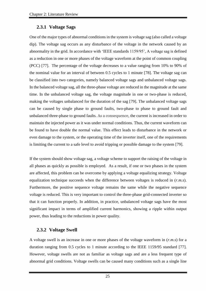
Chapter 2: Literature Review
25
2.3.1 Voltage Sags
One of the major types of abnormal conditions in the system is voltage sag (also called a voltage
dip). The voltage sag occurs as any disturbance of the voltage in the network caused by an
abnormality in the grid. In accordance with ‘IEEE standards 1159/95’, A voltage sag is defined
as a reduction in one or more phases of the voltage waveform at the point of common coupling
(PCC) [77]. The percentage of the voltage decreases to a value ranging from 10% to 90% of
the nominal value for an interval of between 0.5 cycles to 1 minute [78]. The voltage sag can
be classified into two categories, namely balanced voltage sags and unbalanced voltage sags.
In the balanced voltage sag, all the three-phase voltage are reduced in the magnitude at the same
time. In the unbalanced voltage sag, the voltage magnitude in one or two-phase is reduced,
making the voltages unbalanced for the duration of the sag [79]. The unbalanced voltage sags
can be caused by single phase to ground faults, two-phase to phase to ground fault and
unbalanced three-phase to ground faults. As a consequence, the current is increased in order to
maintain the injected power as it was under normal conditions. Thus, the current waveform can
be found to have double the normal value. This effect leads to disturbance in the network or
even damage to the system, or the operating time of the inverter itself, one of the requirements
is limiting the current to a safe level to avoid tripping or possible damage to the system [79].
If the system should show voltage sag, a voltage scheme to support the raising of the voltage in
all phases as quickly as possible is employed. As a result, if one or two phases in the system
are affected, this problem can be overcome by applying a voltage equalizing strategy. Voltage
equalization technique succeeds when the difference between voltages is reduced in (r.m.s).
Furthermore, the positive sequence voltage remains the same while the negative sequence
voltage is reduced. This is very important to control the three-phase grid-connected inverter so
that it can function properly. In addition, in practice, unbalanced voltage sags have the most
significant impact in terms of amplified current harmonics, showing a ripple within output
power, thus leading to the reductions in power quality.
2.3.2 Voltage Swell
A voltage swell is an increase in one or more phases of the voltage waveform in (r.m.s) for a
duration ranging from 0.5 cycles to 1 minute according to the IEEE 1159/95 standard [77].
However, voltage swells are not as familiar as voltage sags and are a less frequent type of
abnormal grid conditions. Voltage swells can be caused many conditions such as a single line

Chapter 2: Literature Review
26
to ground faults or when switching in large capacitor banks, or when large loads are switched
off [80].
2.4 Methods of Decomposition of Positive and Negative
Sequence Components
In the studies described above for power quality, the three-phase grid-connected inverter was
tested under normal grid conditions. Notwithstanding how the control introduces good
performance during normal operation, some important issues regarding the operation of the
three-phase inverter during unbalanced grid conditions have been pointed out. Abnormal grid
conditions can be divided into two main sections. The first section demonstrates balanced fault
when the drop or rise of all three-phase voltage representing the same amplitude. The second
section demonstrates unbalanced fault where the voltage amplitudes are unequal or any changes
of phase shift between the phases due to voltage in one or more phase dropping or rising
suddenly. Under abnormal grid conditions such as voltage sags or voltage swells, the current
injected into the grid loses its sinusoidal and balanced presence.
When unbalanced conditions occur, negative sequence components should appear in the grid
as well as the positive sequence, which is creating a more challenging control system. As a
result, the power inverter needs to change the amplitude or the phase angle of the injected
current in order to ride through the fault during unbalanced voltage conditions. In this case, the
negative sequence component is used to overcome the effect of the fault in the injected current.
Hence, a method of the decomposing the voltage and current into its positive and negative
sequence components is necessary.
A positive voltage sequence is defined as consisting of the balanced three-phase voltage which
is equivalent in magnitude and phase, transferred by 120 degrees rotation at the system
frequency with a phase sequence of normally a, b, c. However, the adverse (negative ) sequence
set is also well-adjusted with three equal magnitude quantities at 120 degrees phase shift
separately with the phase rotation of counter-clockwise or reversed phase sequence a, c, b [29].
Figure 2.2 shows the positive and the negative sequence components.
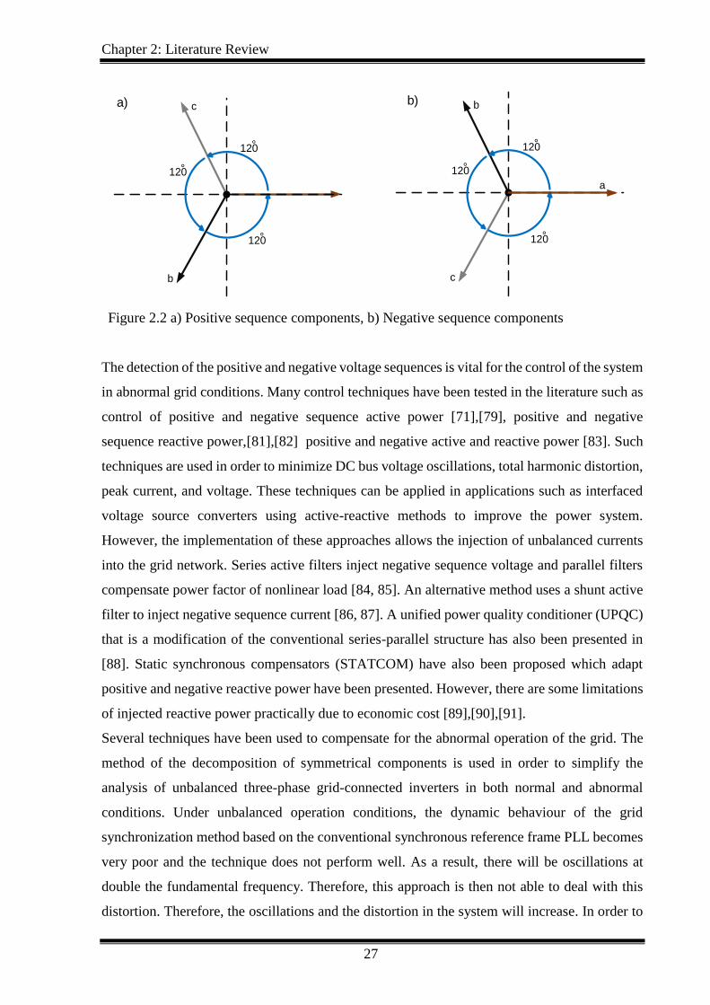
Chapter 2: Literature Review
27
120
°
120
°
120
°
c
b
a
120
°
120
°
120
°
b
c
a) b)
Figure 2.2 a) Positive sequence components, b) Negative sequence components
The detection of the positive and negative voltage sequences is vital for the control of the system
in abnormal grid conditions. Many control techniques have been tested in the literature such as
control of positive and negative sequence active power [71],[79], positive and negative
sequence reactive power,[81],[82] positive and negative active and reactive power [83]. Such
techniques are used in order to minimize DC bus voltage oscillations, total harmonic distortion,
peak current, and voltage. These techniques can be applied in applications such as interfaced
voltage source converters using active-reactive methods to improve the power system.
However, the implementation of these approaches allows the injection of unbalanced currents
into the grid network. Series active filters inject negative sequence voltage and parallel filters
compensate power factor of nonlinear load [84, 85]. An alternative method uses a shunt active
filter to inject negative sequence current [86, 87]. A unified power quality conditioner (UPQC)
that is a modification of the conventional series-parallel structure has also been presented in
[88]. Static synchronous compensators (STATCOM) have also been proposed which adapt
positive and negative reactive power have been presented. However, there are some limitations
of injected reactive power practically due to economic cost [89],[90],[91].
Several techniques have been used to compensate for the abnormal operation of the grid. The
method of the decomposition of symmetrical components is used in order to simplify the
analysis of unbalanced three-phase grid-connected inverters in both normal and abnormal
conditions. Under unbalanced operation conditions, the dynamic behaviour of the grid
synchronization method based on the conventional synchronous reference frame PLL becomes
very poor and the technique does not perform well. As a result, there will be oscillations at
double the fundamental frequency. Therefore, this approach is then not able to deal with this
distortion. Therefore, the oscillations and the distortion in the system will increase. In order to

Chapter 2: Literature Review
28
avoid issues regarding the lack of balance, a few advanced PLLs are applied. In the literature,
there are different advanced grid synchronization approaches based on the most common
decomposition categories such as synchronous reference frame and stationary reference frame
[92], [93], [94].
To deal with these abnormal conditions, an appropriate technique is needed with a specific
strategy that requires the designer to calculate the current that should be injected into the grid
by the grid-connected inverter. However, the implementation of the above approaches allows
the introduction of unbalanced currents within the network. Consequently, specific current
control structures that are able to properly regulate the positive-sequence and negative-sequence
components, are necessary in order to obtain satisfactory results.
2.4.1 Decouple Double Synchronous Reference Frame PLL
Synchronous reference frame (SRF) techniques based on the phase locked loop (PLL) is usually
used in normal grid condition [95],[96]. In this type of method, the three-phase voltage is
converted from the abc reference frame to the synchronous reference frame dq. Nevertheless,
this method cannot be used when unbalanced condition occurs in the system or when there is a
disturbance in the network due to oscillatory errors arising from the negative sequence voltage,
so, the identifiable dynamic behavior will be seen to become progressively worse. In order to
alleviate this concern, the double synchronous reference frame phase locked loop (DSRF-PLL)
has been used [13],[97].
The DSRF-PLL is depended on two synchronous reference frames one for the positive sequence
components and another for the negative voltage sequence components. This method can obtain
the amplitude and the phase angle θ under unbalanced grid conditions into two dq components.
However, this technique gives rise to the oscillation at double the fundamental frequency that
is injected by positive and negative sequence current to the grid. In order to cancel out the
oscillation term, the decoupled double synchronous reference frame phase locked loop (DD-
SRF-PLL) is used [98].
Figure 2.3 shows the decoupled double synchronous reference frame PLL. In this technique, a
cross-decoupling term is added to the double synchronous reference frame. While the DD-SRF
technique shows good performance, the implementation of it is quite complex and the dynamic
response is slow [99]. Overall, this method produces an extra delay in the PLL [100]. Other
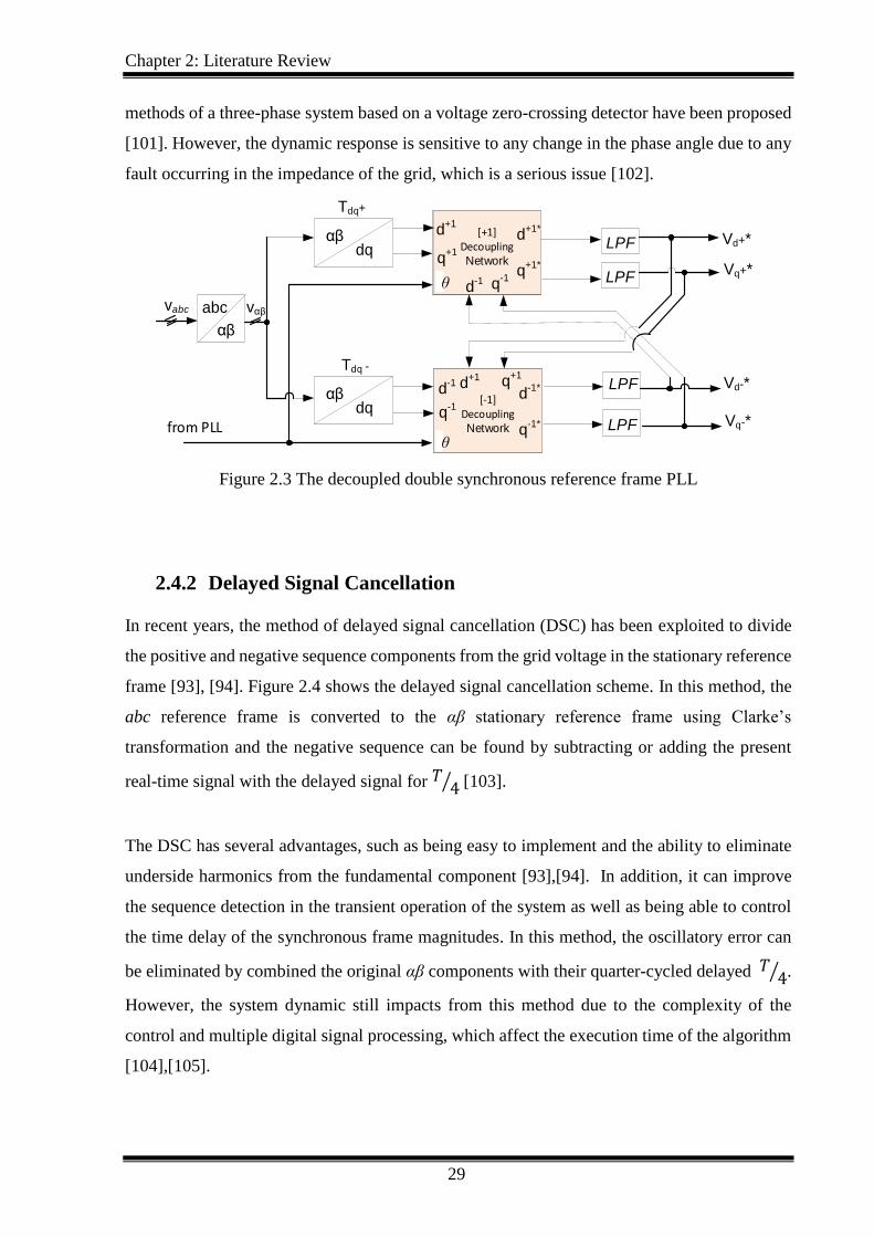
Chapter 2: Literature Review
29
methods of a three-phase system based on a voltage zero-crossing detector have been proposed
[101]. However, the dynamic response is sensitive to any change in the phase angle due to any
fault occurring in the impedance of the grid, which is a serious issue [102].
αβdq
αβdq
Tdq+
abc
αβ
d+1
d+1
d+1
q+1
[+1]Decoupling Network
d+1*
q+1*
d-1 q
-1
d+1
d+1
d-1
q-1
[-1]Decoupling Network
d-1*
q-1*
d+1 q
+1
LPF
LPF
LPF
LPFfrom PLL
Tdq -
vαβ
Vd+*
Vq+*
Vq-*
Vd-*
θ
θ
vabc
Figure 2.3 The decoupled double synchronous reference frame PLL
2.4.2 Delayed Signal Cancellation
In recent years, the method of delayed signal cancellation (DSC) has been exploited to divide
the positive and negative sequence components from the grid voltage in the stationary reference
frame [93], [94]. Figure 2.4 shows the delayed signal cancellation scheme. In this method, the
abc reference frame is converted to the αβ stationary reference frame using Clarke’s
transformation and the negative sequence can be found by subtracting or adding the present
real-time signal with the delayed signal for 𝑇 4⁄ [103].
The DSC has several advantages, such as being easy to implement and the ability to eliminate
underside harmonics from the fundamental component [93],[94]. In addition, it can improve
the sequence detection in the transient operation of the system as well as being able to control
the time delay of the synchronous frame magnitudes. In this method, the oscillatory error can
be eliminated by combined the original αβ components with their quarter-cycled delayed 𝑇 4⁄ .
However, the system dynamic still impacts from this method due to the complexity of the
control and multiple digital signal processing, which affect the execution time of the algorithm
[104],[105].
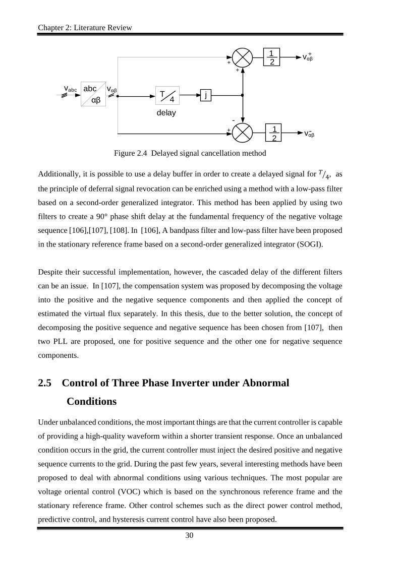
Chapter 2: Literature Review
30
abc
αβ
vαβ
4T
1
1
2
2
vαβ
vαβ
-
-
+
+
+
+
delay
jvabc
Figure 2.4 Delayed signal cancellation method
Additionally, it is possible to use a delay buffer in order to create a delayed signal for 𝑇 4⁄ , as
the principle of deferral signal revocation can be enriched using a method with a low-pass filter
based on a second-order generalized integrator. This method has been applied by using two
filters to create a 90° phase shift delay at the fundamental frequency of the negative voltage
sequence [106],[107], [108]. In [106], A bandpass filter and low-pass filter have been proposed
in the stationary reference frame based on a second-order generalized integrator (SOGI).
Despite their successful implementation, however, the cascaded delay of the different filters
can be an issue. In [107], the compensation system was proposed by decomposing the voltage
into the positive and the negative sequence components and then applied the concept of
estimated the virtual flux separately. In this thesis, due to the better solution, the concept of
decomposing the positive sequence and negative sequence has been chosen from [107], then
two PLL are proposed, one for positive sequence and the other one for negative sequence
components.
2.5 Control of Three Phase Inverter under Abnormal
Conditions
Under unbalanced conditions, the most important things are that the current controller is capable
of providing a high-quality waveform within a shorter transient response. Once an unbalanced
condition occurs in the grid, the current controller must inject the desired positive and negative
sequence currents to the grid. During the past few years, several interesting methods have been
proposed to deal with abnormal conditions using various techniques. The most popular are
voltage oriental control (VOC) which is based on the synchronous reference frame and the
stationary reference frame. Other control schemes such as the direct power control method,
predictive control, and hysteresis current control have also been proposed.
Chapter 2: Literature Review
31
A vector control approach was proposed for the first time for a grid rectifier under abnormal
grid conditions to derive positive and negative current sequences in 1996 by Rioual et al.[109].
In this work, only a PI current controller was implemented in the synchronous reference frame
to control the positive sequence in case of abnormal grid conditions in order to track positive
and negative sequence components. Nevertheless, one of the main drawbacks of this type of
the control is that the negative sequence voltage during unbalance conditions cannot work
properly with this control due to the limitation of the bandwidth. Therefore, in 1999, a
combination of two sequence components with the DC link voltage controller in the dq
synchronous reference frame has been proposed [110]. The proposed method has a dual current
control scheme for the positive and negative sequence currents. The technique is able to reduce
the steady state error compared with single current control. However, this method is used when
operating the grid-connected inverter only in steady-state conditions and it cannot be applied
under unbalanced supply conditions due to limitations in the dynamics of the system.
In another subsequent method, one PI controller was used with resonant (R) instead of dual
current controllers allowing a rectifier to generate a dc output under unbalanced grid conditions
at double frequency [111]. However, eliminating a steady state error at twice of the fundamental
frequency was one of the main critical issues.
In addition, vector control technique has been used in a distributed generation (DG) inverters
under abnormal grid operation conditions [112]. Optimum power quality characteristics were
achieved, under unbalanced grid voltages. This research focused on many important aspects,
such as DC voltage optimization and maximum power exchange, and also a combination of the
different methods called a hybrid strategy was described.
Control of the three-phase grid-connected inverter during unbalanced grid conditions using
direct power control based on instantaneous active and reactive power has also been proposed.
Other research proposed a new concept for selecting active power quality characteristics based
on a fast current controller and a rearrange reference current during unsymmetrical voltage
[113]. Similar research has proposed reactive power control based on symmetrical component
[114]. Another study finding a higher smoothing active and reactive power characteristics using
a method previously for selecting active power quality characteristics [115].

Chapter 2: Literature Review
32
On the other hand, vector control method during unbalanced gird condition needs double
reference synchronization frames for the positive and negative sequences transformation
modules for voltage and current. However, PI controller has some drawbacks such as:
Four PI controllers should be implemented for the positive and negative sequences
based on the double synchronous reference frame which will increase the complexity
and computational load
In the PI controller, grid synchronization can be achieved with two PLLs using one for
the positive sequence components of the voltage and another one of the negative voltage
sequence.
As an alternative method to PI current control based on the double synchronous reference
frame, proportional-resonant controllers can extend the operation on stationary reference α-β
rotating frame to control the current injected by the grid-connected power converter under
abnormal grid conditions [116]. In this control scheme, the output currents are converted to the
stationary reference frames that results in two AC current signals to be controlled [112, 117].
This type of control is based on frequency adaptive filters. These filters give the same
performance for both positive and negative frequencies [62], [118]. In addition, the multiple d-
q rotations become unnecessary.
It can be said that there are many advantages of using PR controller including:
We do not require additional controllers for the positive and negative sequence currents.
Synchronization can be achieved with one PLL using the positive sequence component
of the voltage.
Only one PR controller can regulate positive and negative sequences (+ω and –ω)
Only the positive sequence angle needs to be synchronized.
Based on current control approaches, the current injected into the grid by the three-phase
inverter should follow different strategies in unbalance grid conditions at the point of common
coupling (PCC). In the literature, different control approaches are used to meet the requirement
of control under abnormal conditions and to enhance the system’s response [79]. The first
approach is instantaneous unity power factor control (IUPFC). This method of control is
essential to be used if the injected current vector is required to follow the voltage vector. A
second approach is average unity power factor control (AUPFC). In this strategy, the harmonics
can be reduced, resulting in a lower THD.

Chapter 2: Literature Review
33
A further method is instantaneous active reactive control (IARC). This method is more useful
in control active and reactive power based on p-q theory. In this type of method, both active
and reactive power is controlled instantaneously since the current vector is aligned with voltage
vector as well as any orthogonal components. However, the voltage vector has oscillations at
twice the fundamental grid frequency that increases the harmonics into the grid [29].
To overcome these drawbacks another strategy has been proposed, called the positive and
negative sequence control (PNSC). This strategy can deal with the current control under
unbalanced conditions. Here, both positive and negative sequence current control is applied in
the system. This method can be used in the synchronous reference frame using dual PI
controllers. However, one of the issues can be that when the reactive power not considered, the
oscillation term of q will not appear.
In the balance positive sequence control (BPSC) method a balanced sinusoidal waveform is
injected by applying positive sequence control to the grid during unbalanced conditions. There
are many advantages of this strategy, such as improving the power quality of the system by
allowing the current waveform to be symmetrical during unbalanced conditions. In addition, it
is a simple method since only the positive sequence angle needs to be synchronized. This
method can be easily applied to stationary reference frame using PR controller while needs
double synchronous reference frame using dual PI controllers. This method is the only one can
obtain the balanced current among other strategies [29].
2.6 Advanced Intelligent Optimization Methods
Beside conventional control techniques, many intelligent advanced control methods have been
successfully applied. One of these control advanced methods is based on a self-commissioning
tuning process using advanced optimization algorithms which tune the parameters of the
controllers to manage different normal and abnormal conditions and the transitions among
them. PI and PR controllers have been widely used for speed and position control in many
various applications.
Conventionally, the tuning of these controllers may be accomplished with the most method
using a trial-and-error principle. In addition, tuning can also be achieved using many
algorithmic methods, including Ziegler-Nichols, root locus, and pole placement techniques.
The controller parameters can be tuned in a similar way based on the root locus of the system
[119]. The Ziegler-Nichols method is the most well-known, but it might not provide good
tuning and tends to produce an overshoot. Moreover, it takes more time to achieve control and
Chapter 2: Literature Review
34
reduces the stability of the system. Not only that, but the operator is required to be very familiar
with the characteristics and parameters of the system. In addition, such techniques can take
significant time to achieve an optimum solution [120].
For this reason and to enhance the robustness and increase the performance of the traditional
parameter-tuning techniques, artificial intelligent optimization (AIO) methods are used, such
as artificial neural networks (ANN), fuzzy logic (FL), genetic algorithms (GA) and particle
swarm optimization (PSO). Such approaches can be necessary to regulate the parameters of the
controller and improve the performance [121, 122]. AIO has been used in many applications
such as the drive application, machine design, and fault detection. PSO is one of the most widely
used methods in advanced optimization control due to an effective and powerful technique for
solving a problem.
Compared to GA and ANN, PSO can operate much more easily and faster to optimize, making
it well suited for real-time control applications which experience time-varying disturbances.
Moreover, it is a stable optimization method that is relatively easy to implement, because there
are few parameters to adjust and it does not impose a significant computational burden to the
microcontroller [123, 124]. Unlike GA, PSO has no complicated evolution operatives such as
crossover and mutation [125].
PSO algorithm is a stochastic search technique that uses a population or swarm of individual
elements which are called particles. Each particle shows independent achievement solution to
a problem and adjusts its own flying experience in the boundary space. In order to determine
the optimal solution of an objective function, each particle has two main variables which
represent a group of parameters to identify the current position 𝑖(𝑡) and current velocity 𝑖(𝑡).
The best previous position is shown the best minimum fitness value of any particle in the
neighbourhood which is recorded and represented as new = 𝑥1, 𝑥2, 𝑥3, … , 𝑥𝑖 and this is called
Personal Best 𝑃𝑏𝑒𝑠𝑡. The index of the best particle among all particles in the population group
called Global Best 𝐺𝑏𝑒𝑠𝑡 and to be encountered by the 𝑖𝑡ℎ particle is a point in domain space
(S).
PSO can be designed based on three main stages:
I. Assessing the fitness value of each particle.
II. Updating local and global best fitness and positions.
III. Every particle can update its own velocity and position.
Chapter 2: Literature Review
35
Several studies have used PSO in different areas. In 1995, PSO was proposed by James
Kennedy and Russell C. Eberhart as a stochastic algorithm based on deterministic points of
natural selection [126]. They proposed an algorithm which is based on intelligent methods that
simulate the social behaviour of the domains posed in animals and plants, such as bird flocking
and swarm theory [126]. They observed that every particle is a part of the neighbourhood
particles that indicate the best particle. However, the performance still in it is early stages and
needs more improvement. Shi and Eberhart added a new parameter called inertia in order to
improve the performance of particle swarm optimization [127]. Another study investigated in
detail the PSO algorithm [128], and It was proven that each particle of the PSO represents a
potential solution to a problem and adjusts its own “flying experience” in a defined boundary
space. Later, several applications have used PSO, such as to optimize the geometry of an
antenna [129],[130]. Recently, this technique has been successfully applied in power
electronics applications [131], [132], including the maximum MPPT of photovoltaic systems
[133], micro-grid voltage source inverters [134] and the PI controller grid-connected inverter
with LC filter [132].
The PSO algorithm is employed for self-tuning parameters where an optimum solution is
determined by using the integral time absolute error (ITAE) as a cost function. The most
commonly utilized cost functions are integral-based such as the ITAE, the integral of squared
error (ISE) and integral of time multiplied by squared error (ITSE) [135], [136]. In the current
research, the ITAE is used:
𝐼𝑇𝐸𝐴 = ∫ 𝑡|𝑒(𝑡)|𝑑𝑡∞
0
(2.8)
Where e(t) is the difference between the reference and actual values. The cost function is
minimised using the current control method such as PI and PR controllers throughout the
optimisation process. A block diagram of the optimization process is shown in Figure 2.5.
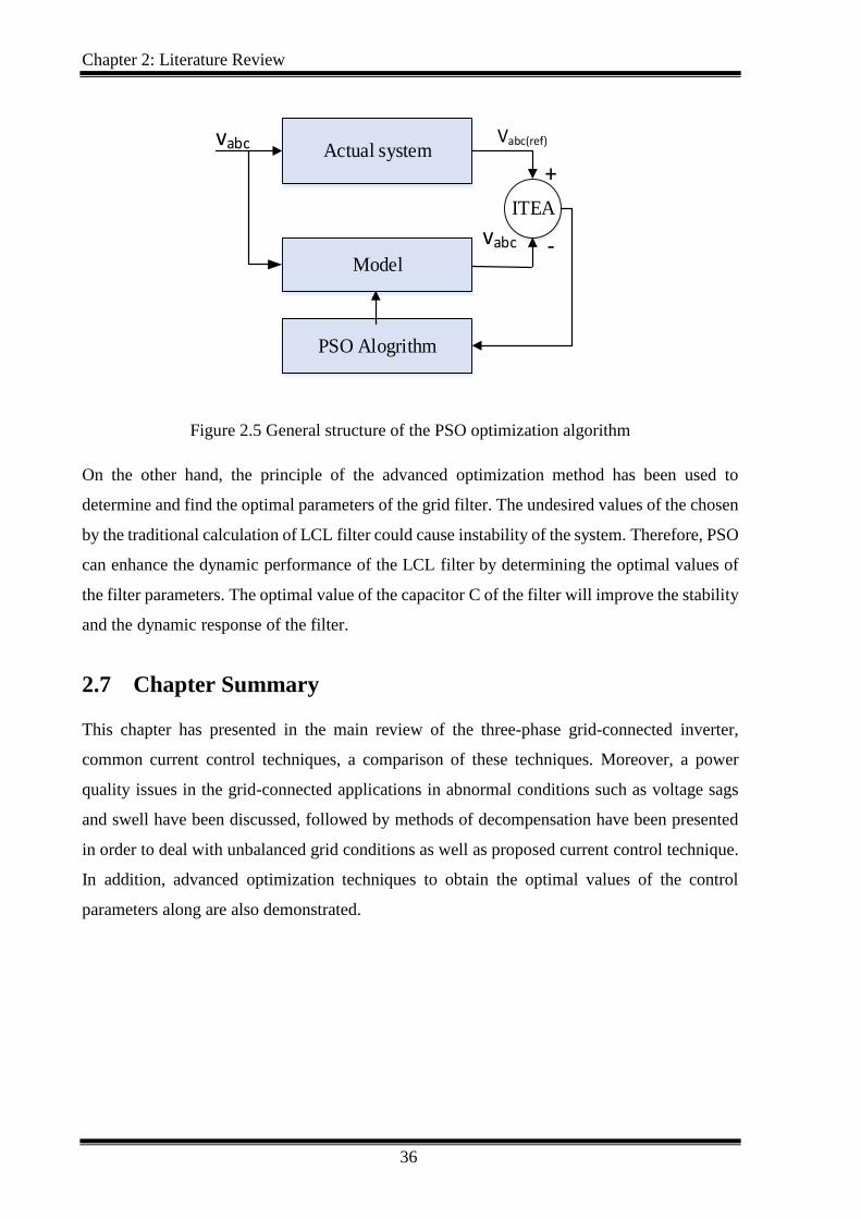
Chapter 2: Literature Review
36
Actual system
Model
PSO Alogrithm
ITEA
+
-
vabc Vabc(ref)
vabc
Figure 2.5 General structure of the PSO optimization algorithm
On the other hand, the principle of the advanced optimization method has been used to
determine and find the optimal parameters of the grid filter. The undesired values of the chosen
by the traditional calculation of LCL filter could cause instability of the system. Therefore, PSO
can enhance the dynamic performance of the LCL filter by determining the optimal values of
the filter parameters. The optimal value of the capacitor C of the filter will improve the stability
and the dynamic response of the filter.
2.7 Chapter Summary
This chapter has presented in the main review of the three-phase grid-connected inverter,
common current control techniques, a comparison of these techniques. Moreover, a power
quality issues in the grid-connected applications in abnormal conditions such as voltage sags
and swell have been discussed, followed by methods of decompensation have been presented
in order to deal with unbalanced grid conditions as well as proposed current control technique.
In addition, advanced optimization techniques to obtain the optimal values of the control
parameters along are also demonstrated.
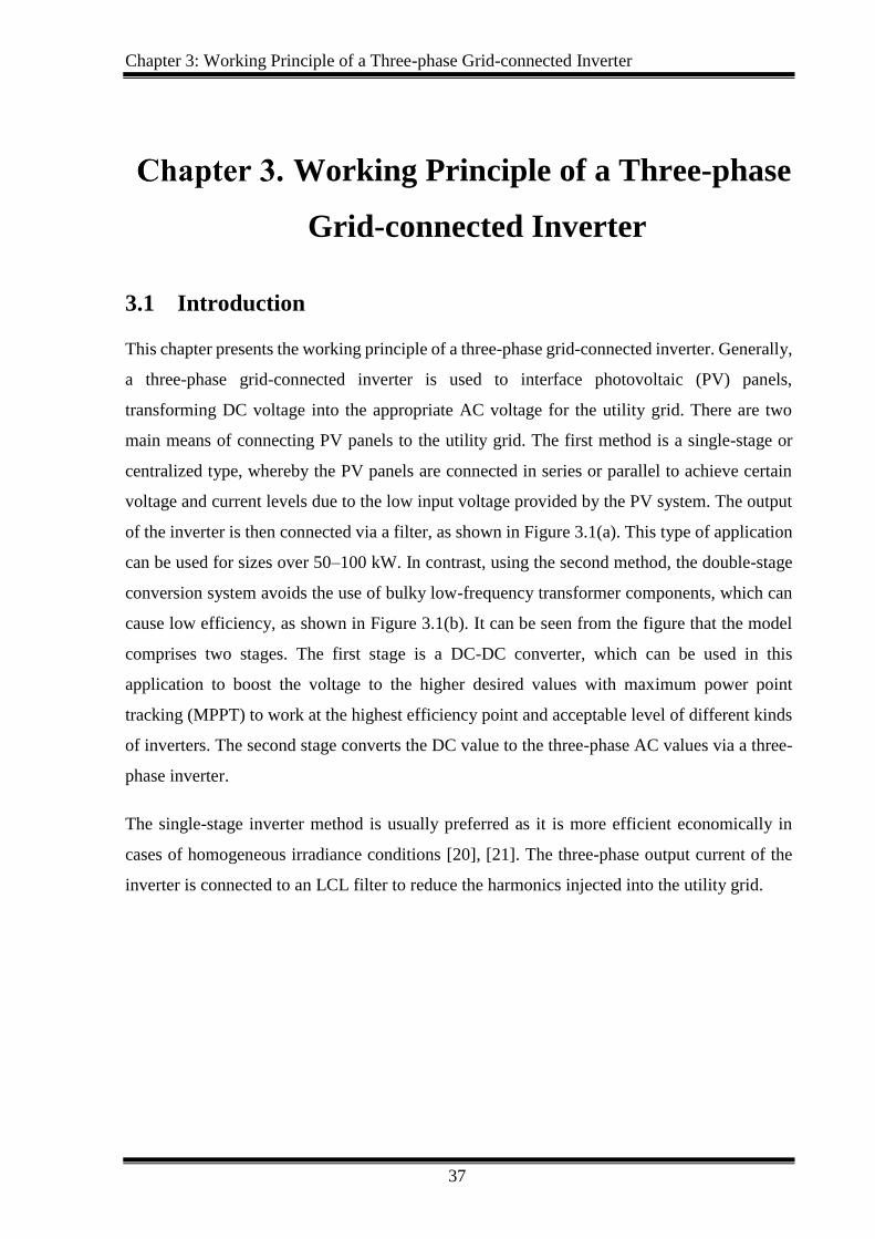
Chapter 3: Working Principle of a Three-phase Grid-connected Inverter
37
Working Principle of a Three-phase
Grid-connected Inverter
3.1 Introduction
This chapter presents the working principle of a three-phase grid-connected inverter. Generally,
a three-phase grid-connected inverter is used to interface photovoltaic (PV) panels,
transforming DC voltage into the appropriate AC voltage for the utility grid. There are two
main means of connecting PV panels to the utility grid. The first method is a single-stage or
centralized type, whereby the PV panels are connected in series or parallel to achieve certain
voltage and current levels due to the low input voltage provided by the PV system. The output
of the inverter is then connected via a filter, as shown in Figure 3.1(a). This type of application
can be used for sizes over 50–100 kW. In contrast, using the second method, the double-stage
conversion system avoids the use of bulky low-frequency transformer components, which can
cause low efficiency, as shown in Figure 3.1(b). It can be seen from the figure that the model
comprises two stages. The first stage is a DC-DC converter, which can be used in this
application to boost the voltage to the higher desired values with maximum power point
tracking (MPPT) to work at the highest efficiency point and acceptable level of different kinds
of inverters. The second stage converts the DC value to the three-phase AC values via a three-
phase inverter.
The single-stage inverter method is usually preferred as it is more efficient economically in
cases of homogeneous irradiance conditions [20], [21]. The three-phase output current of the
inverter is connected to an LCL filter to reduce the harmonics injected into the utility grid.
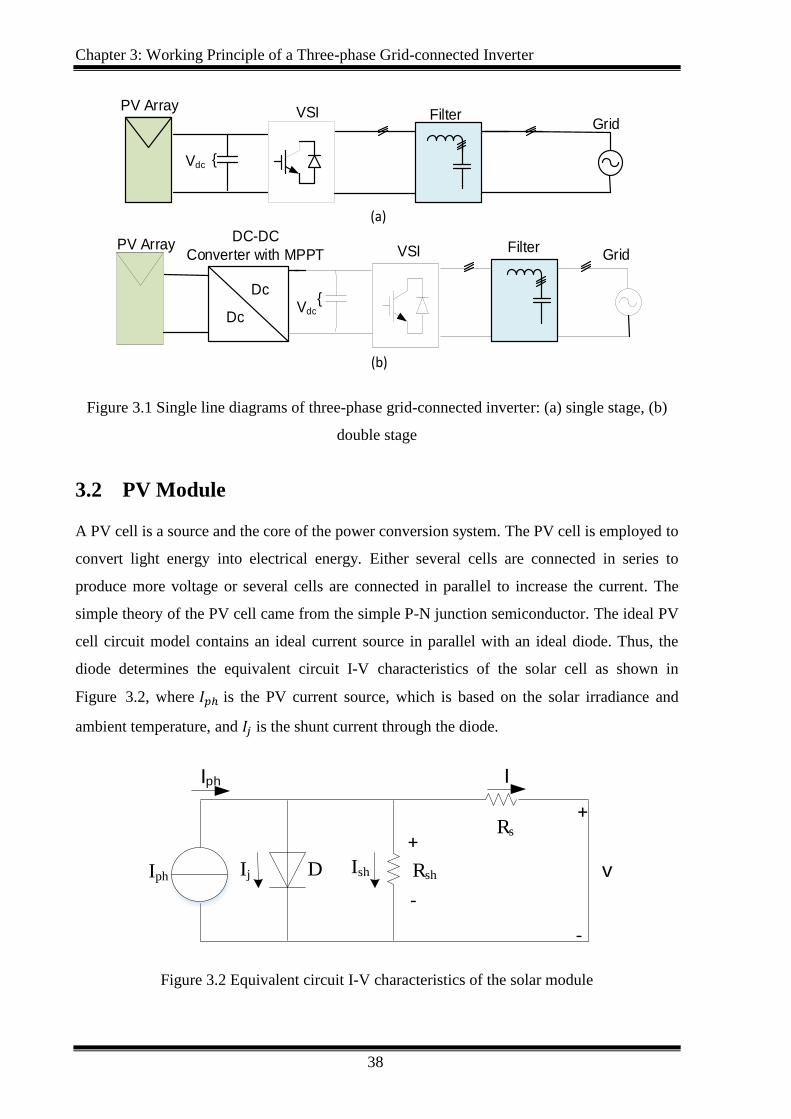
Chapter 3: Working Principle of a Three-phase Grid-connected Inverter
38
Vdc
PV Array
GridFilterVSI
(a)
(b)
Vdc
VSIDC-DC
Converter with MPPT
Dc
Dc
GridFilterPV Array
Figure 3.1 Single line diagrams of three-phase grid-connected inverter: (a) single stage, (b)
double stage
3.2 PV Module
A PV cell is a source and the core of the power conversion system. The PV cell is employed to
convert light energy into electrical energy. Either several cells are connected in series to
produce more voltage or several cells are connected in parallel to increase the current. The
simple theory of the PV cell came from the simple P-N junction semiconductor. The ideal PV
cell circuit model contains an ideal current source in parallel with an ideal diode. Thus, the
diode determines the equivalent circuit I-V characteristics of the solar cell as shown in
Figure 3.2, where 𝐼𝑝ℎ is the PV current source, which is based on the solar irradiance and
ambient temperature, and 𝐼𝑗 is the shunt current through the diode.
Iph I
+
-
Rs
Rsh v
+
-
IshIj DIph
Figure 3.2 Equivalent circuit I-V characteristics of the solar module
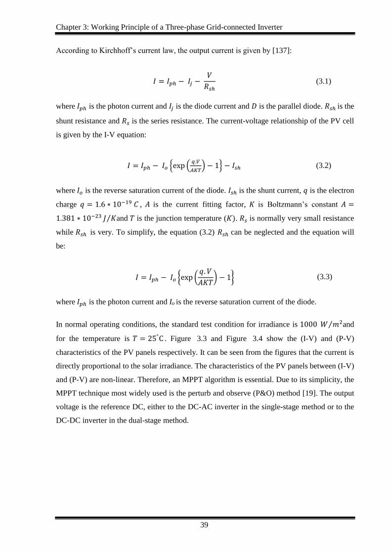
Chapter 3: Working Principle of a Three-phase Grid-connected Inverter
39
According to Kirchhoff’s current law, the output current is given by [137]:
𝐼 = 𝐼𝑝ℎ − 𝐼𝑗 − 𝑉
𝑅𝑠ℎ (3.1)
where 𝐼𝑝ℎ is the photon current and 𝐼𝑗 is the diode current and 𝐷 is the parallel diode. 𝑅𝑠ℎ is the
shunt resistance and 𝑅𝑠 is the series resistance. The current-voltage relationship of the PV cell
is given by the I-V equation:
𝐼 = 𝐼𝑝ℎ − 𝐼𝑜 exp (𝑞.𝑉
𝐴𝐾𝑇) − 1 − 𝐼𝑠ℎ (3.2)
where 𝐼𝑜 is the reverse saturation current of the diode. 𝐼𝑠ℎ is the shunt current, 𝑞 is the electron
charge 𝑞 = 1.6 ∗ 10−19 𝐶 , 𝐴 is the current fitting factor, 𝐾 is Boltzmann’s constant 𝐴 =
1.381 ∗ 10−23 𝐽 𝐾⁄ and 𝑇 is the junction temperature (𝐾). 𝑅𝑠 is normally very small resistance
while 𝑅𝑠ℎ is very. To simplify, the equation (3.2) 𝑅𝑠ℎ can be neglected and the equation will
be:
𝐼 = 𝐼𝑝ℎ − 𝐼𝑜 exp (𝑞. 𝑉
𝐴𝐾𝑇) − 1 (3.3)
where 𝐼𝑝ℎ is the photon current and Io is the reverse saturation current of the diode.
In normal operating conditions, the standard test condition for irradiance is 1000 𝑊 𝑚2⁄ and
for the temperature is 𝑇 = 25°C . Figure 3.3 and Figure 3.4 show the (I-V) and (P-V)
characteristics of the PV panels respectively. It can be seen from the figures that the current is
directly proportional to the solar irradiance. The characteristics of the PV panels between (I-V)
and (P-V) are non-linear. Therefore, an MPPT algorithm is essential. Due to its simplicity, the
MPPT technique most widely used is the perturb and observe (P&O) method [19]. The output
voltage is the reference DC, either to the DC-AC inverter in the single-stage method or to the
DC-DC inverter in the dual-stage method.
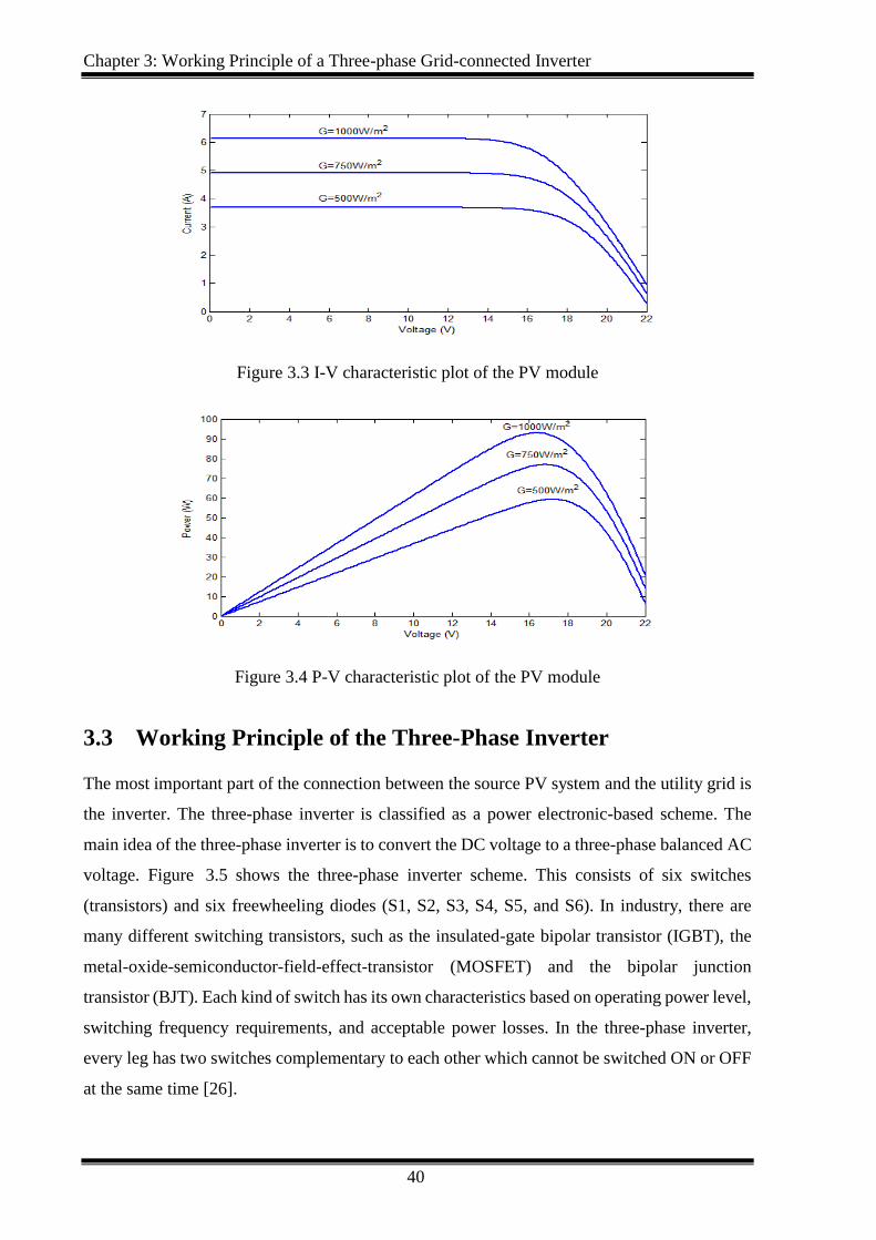
Chapter 3: Working Principle of a Three-phase Grid-connected Inverter
40
Figure 3.3 I-V characteristic plot of the PV module
Figure 3.4 P-V characteristic plot of the PV module
3.3 Working Principle of the Three-Phase Inverter
The most important part of the connection between the source PV system and the utility grid is
the inverter. The three-phase inverter is classified as a power electronic-based scheme. The
main idea of the three-phase inverter is to convert the DC voltage to a three-phase balanced AC
voltage. Figure 3.5 shows the three-phase inverter scheme. This consists of six switches
(transistors) and six freewheeling diodes (S1, S2, S3, S4, S5, and S6). In industry, there are
many different switching transistors, such as the insulated-gate bipolar transistor (IGBT), the
metal-oxide-semiconductor-field-effect-transistor (MOSFET) and the bipolar junction
transistor (BJT). Each kind of switch has its own characteristics based on operating power level,
switching frequency requirements, and acceptable power losses. In the three-phase inverter,
every leg has two switches complementary to each other which cannot be switched ON or OFF
at the same time [26].
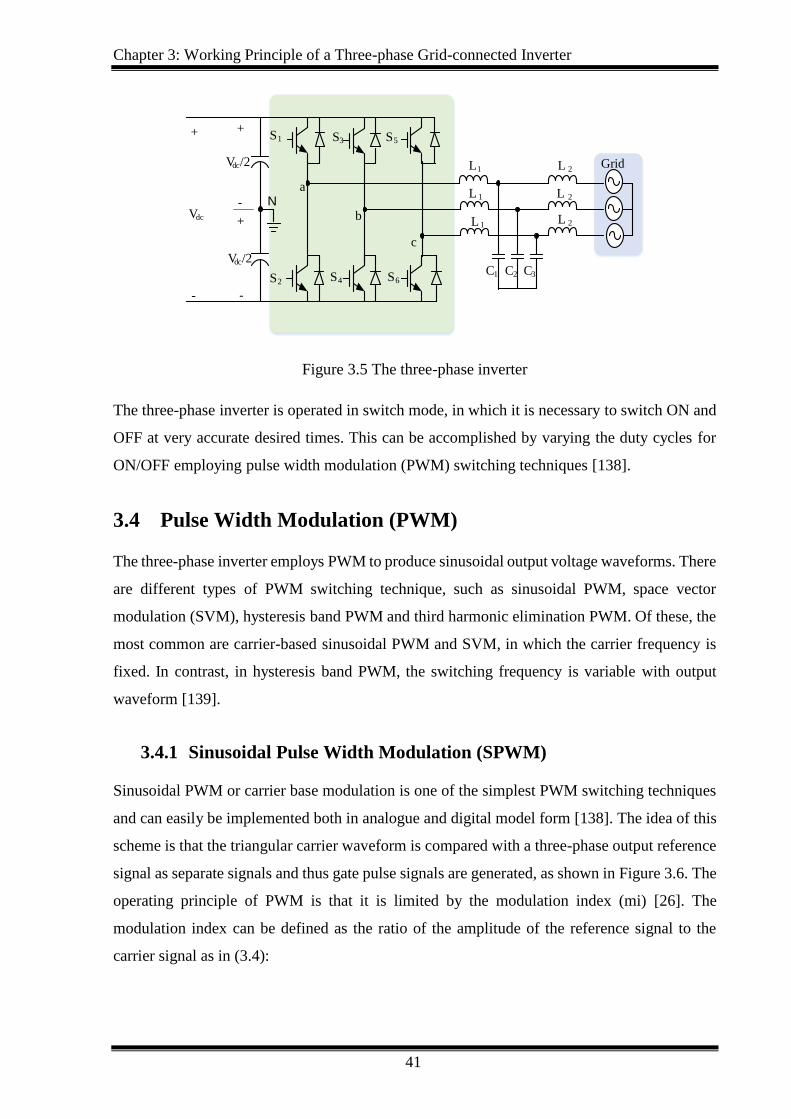
Chapter 3: Working Principle of a Three-phase Grid-connected Inverter
41
- -
+
Vdc
L1
L 1
L1
C1 C3C2
Grid
a
b
c
L 2
L 2
L 2
+
+
-
Vdc/2
Vdc/2
N
S1
S2
S3
S4
S5
S6
Figure 3.5 The three-phase inverter
The three-phase inverter is operated in switch mode, in which it is necessary to switch ON and
OFF at very accurate desired times. This can be accomplished by varying the duty cycles for
ON/OFF employing pulse width modulation (PWM) switching techniques [138].
3.4 Pulse Width Modulation (PWM)
The three-phase inverter employs PWM to produce sinusoidal output voltage waveforms. There
are different types of PWM switching technique, such as sinusoidal PWM, space vector
modulation (SVM), hysteresis band PWM and third harmonic elimination PWM. Of these, the
most common are carrier-based sinusoidal PWM and SVM, in which the carrier frequency is
fixed. In contrast, in hysteresis band PWM, the switching frequency is variable with output
waveform [139].
3.4.1 Sinusoidal Pulse Width Modulation (SPWM)
Sinusoidal PWM or carrier base modulation is one of the simplest PWM switching techniques
and can easily be implemented both in analogue and digital model form [138]. The idea of this
scheme is that the triangular carrier waveform is compared with a three-phase output reference
signal as separate signals and thus gate pulse signals are generated, as shown in Figure 3.6. The
operating principle of PWM is that it is limited by the modulation index (mi) [26]. The
modulation index can be defined as the ratio of the amplitude of the reference signal to the
carrier signal as in (3.4):
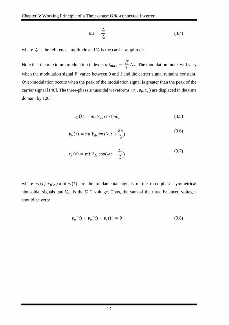
Chapter 3: Working Principle of a Three-phase Grid-connected Inverter
42
𝑚𝑖 = 𝑉𝑟
𝑉𝑐 (3.4)
where 𝑉𝑟 is the reference amplitude and 𝑉𝑐 is the carrier amplitude.
Note that the maximum modulation index is 𝑚𝑖𝑚𝑎𝑥 = √3
2𝑉𝑑𝑐. The modulation index will vary
when the modulation signal 𝑉𝑟 varies between 0 and 1 and the carrier signal remains constant.
Over-modulation occurs when the peak of the modulation signal is greater than the peak of the
carrier signal [140]. The three-phase sinusoidal waveforms (𝑣𝑎, 𝑣𝑏 , 𝑣𝑐) are displaced in the time
domain by 120°:
𝑣𝑎(𝑡) = 𝑚𝑖 𝑉𝑑𝑐 cos(𝜔𝑡) (3.5)
𝑣𝑏(𝑡) = 𝑚𝑖 𝑉𝑑𝑐 cos(𝜔𝑡 +2𝜋
3)
(3.6)
𝑣𝑐(𝑡) = 𝑚𝑖 𝑉𝑑𝑐 cos(𝜔𝑡 −2𝜋
3)
(3.7)
where 𝑣𝑎(𝑡), 𝑣𝑏(𝑡) and 𝑣𝑐(𝑡) are the fundamental signals of the three-phase symmetrical
sinusoidal signals and 𝑉𝑑𝑐 is the D.C voltage. Thus, the sum of the three balanced voltages
should be zero:
𝑣𝑎(𝑡) + 𝑣𝑏(𝑡) + 𝑣𝑐(𝑡) = 0 (3.8)
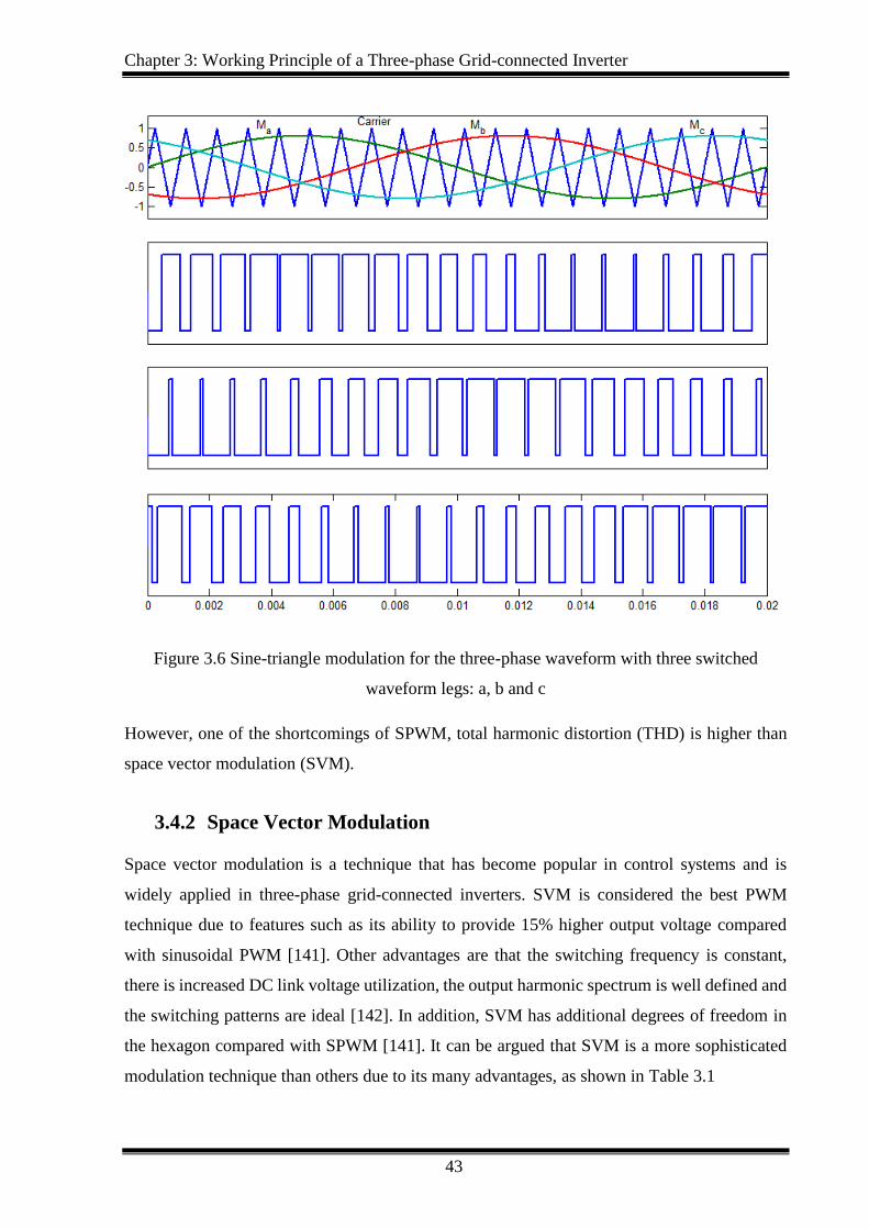
Chapter 3: Working Principle of a Three-phase Grid-connected Inverter
43
Figure 3.6 Sine-triangle modulation for the three-phase waveform with three switched
waveform legs: a, b and c
However, one of the shortcomings of SPWM, total harmonic distortion (THD) is higher than
space vector modulation (SVM).
3.4.2 Space Vector Modulation
Space vector modulation is a technique that has become popular in control systems and is
widely applied in three-phase grid-connected inverters. SVM is considered the best PWM
technique due to features such as its ability to provide 15% higher output voltage compared
with sinusoidal PWM [141]. Other advantages are that the switching frequency is constant,
there is increased DC link voltage utilization, the output harmonic spectrum is well defined and
the switching patterns are ideal [142]. In addition, SVM has additional degrees of freedom in
the hexagon compared with SPWM [141]. It can be argued that SVM is a more sophisticated
modulation technique than others due to its many advantages, as shown in Table 3.1
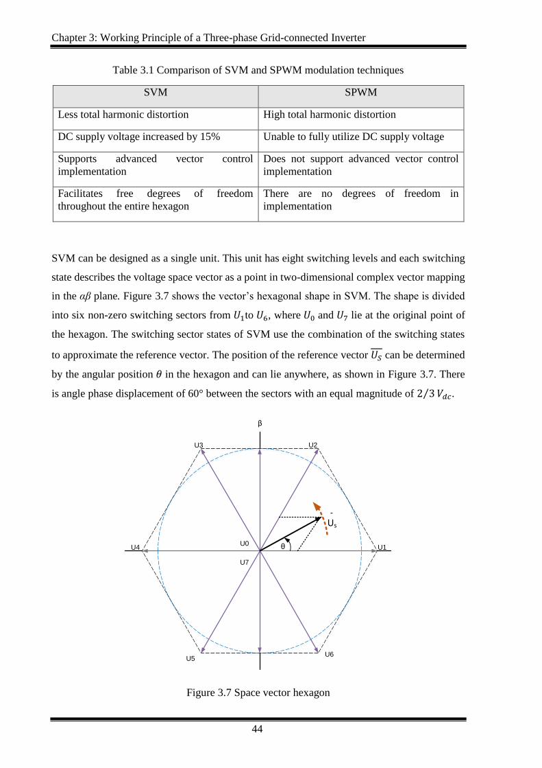
Chapter 3: Working Principle of a Three-phase Grid-connected Inverter
44
Table 3.1 Comparison of SVM and SPWM modulation techniques
SVM SPWM
Less total harmonic distortion High total harmonic distortion
DC supply voltage increased by 15% Unable to fully utilize DC supply voltage
Supports advanced vector control
implementation
Does not support advanced vector control
implementation
Facilitates free degrees of freedom
throughout the entire hexagon
There are no degrees of freedom in
implementation
SVM can be designed as a single unit. This unit has eight switching levels and each switching
state describes the voltage space vector as a point in two-dimensional complex vector mapping
in the αβ plane. Figure 3.7 shows the vector’s hexagonal shape in SVM. The shape is divided
into six non-zero switching sectors from 𝑈1to 𝑈6, where 𝑈0 and 𝑈7 lie at the original point of
the hexagon. The switching sector states of SVM use the combination of the switching states
to approximate the reference vector. The position of the reference vector 𝑈𝑆 can be determined
by the angular position 𝜃 in the hexagon and can lie anywhere, as shown in Figure 3.7. There
is angle phase displacement of 60° between the sectors with an equal magnitude of 2 3⁄ 𝑉𝑑𝑐.
U2 U3
U5 U6
θ
Us
-
β
U7
U0 U1 U4
Figure 3.7 Space vector hexagon
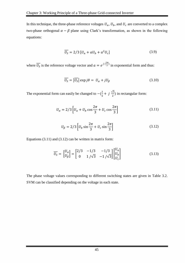
Chapter 3: Working Principle of a Three-phase Grid-connected Inverter
45
In this technique, the three-phase reference voltages 𝑈𝑎, 𝑈𝑏, and 𝑈𝑐 are converted to a complex
two-phase orthogonal 𝛼 − 𝛽 plane using Clark’s transformation, as shown in the following
equations:
𝑈𝑆 = 2 3⁄ [𝑈𝑎 + 𝑎𝑈𝑏 + 𝑎2𝑈𝑐] (3.9)
where 𝑈𝑆 is the reference voltage vector and 𝑎 = 𝑒𝑗 (2𝜋
3) in exponential form and thus:
𝑈𝑆 = |𝑈𝑆| exp 𝑗𝜃 = 𝑈𝛼 + 𝑗𝑈𝛽 (3.10)
The exponential form can easily be changed to −(1
2+ 𝑗
√3
2) in rectangular form:
𝑈𝛼 = 2 3⁄ [𝑈𝑎 + 𝑈𝑏 cos2𝜋
3+ 𝑈𝑐 cos
2𝜋
3] (3.11)
𝑈𝛽 = 2 3⁄ [𝑈𝑏 sin2𝜋
3+ 𝑈𝑐 sin
2𝜋
3] (3.12)
Equations (3.11) and (3.12) can be written in matrix form:
𝑈𝑆 = [𝑈𝛼
𝑈𝛽] = [
2/3 −1/3 −1/3
0 1 /√3 −1 /√3] [
𝑈𝑎
𝑈𝑏
𝑈𝑐
] (3.13)
The phase voltage values corresponding to different switching states are given in Table 3.2.
SVM can be classified depending on the voltage in each state.
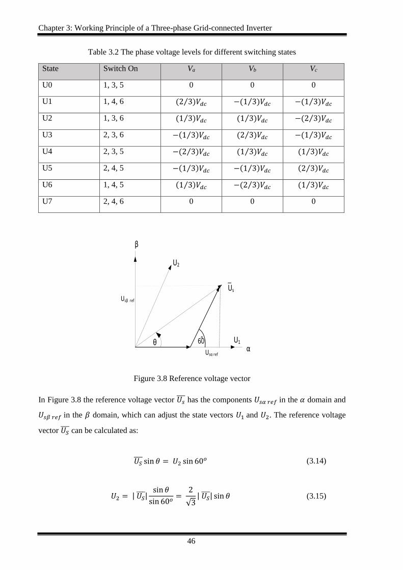
Chapter 3: Working Principle of a Three-phase Grid-connected Inverter
46
Table 3.2 The phase voltage levels for different switching states
State Switch On Va Vb Vc
U0 1, 3, 5 0 0 0
U1 1, 4, 6 (2 3⁄ )𝑉𝑑𝑐 −(1 3⁄ )𝑉𝑑𝑐 −(1 3⁄ )𝑉𝑑𝑐
U2 1, 3, 6 (1 3⁄ )𝑉𝑑𝑐 (1 3⁄ )𝑉𝑑𝑐 −(2 3⁄ )𝑉𝑑𝑐
U3 2, 3, 6 −(1 3⁄ )𝑉𝑑𝑐 (2 3⁄ )𝑉𝑑𝑐 −(1 3⁄ )𝑉𝑑𝑐
U4 2, 3, 5 −(2 3⁄ )𝑉𝑑𝑐 (1 3⁄ )𝑉𝑑𝑐 (1 3⁄ )𝑉𝑑𝑐
U5 2, 4, 5 −(1 3⁄ )𝑉𝑑𝑐 −(1 3⁄ )𝑉𝑑𝑐 (2 3⁄ )𝑉𝑑𝑐
U6 1, 4, 5 (1 3⁄ )𝑉𝑑𝑐 −(2 3⁄ )𝑉𝑑𝑐 (1 3⁄ )𝑉𝑑𝑐
U7 2, 4, 6 0 0 0
U2
θ
Us
β
α60 °
Usα ref
U1
Usβ ref
Figure 3.8 Reference voltage vector
In Figure 3.8 the reference voltage vector 𝑈𝑠 has the components 𝑈𝑠𝛼 𝑟𝑒𝑓 in the 𝛼 domain and
𝑈𝑠𝛽 𝑟𝑒𝑓 in the 𝛽 domain, which can adjust the state vectors 𝑈1 and 𝑈2. The reference voltage
vector 𝑈𝑆 can be calculated as:
𝑈𝑆 sin 𝜃 = 𝑈2 sin 60𝜊 (3.14)
𝑈2 = | 𝑈𝑆 |
sin 𝜃
sin 60𝜊=
2
√3| 𝑈𝑆 | sin 𝜃 (3.15)
Chapter 3: Working Principle of a Three-phase Grid-connected Inverter
47
𝑈1 = | 𝑈𝑆 | cos 𝜃 − 𝑈2 cos 60𝜊 (3.16)
𝑈1 = | 𝑈𝑆 | cos 𝜃 −
2
√3| 𝑈𝑆 | sin 𝜃 cos 60𝜊 (3.17)
𝑈1 = | 𝑈𝑆 |
2
√3(
√3
2cos 𝜃 − sin 𝜃 cos 60𝜊) (3.18)
𝑈1 = | 𝑈𝑆 |
2
√3( 𝑠𝑖𝑛60𝜊 cos 𝜃 − sin 𝜃 cos 60𝜊) (3.19)
𝑈1 = 2
√3| 𝑈𝑆 | sin(60° − 𝜃) (3.20)
𝑈2 = 2
√3| 𝑈𝑆 | sin(𝜃) (3.21)
3.4.3 Hysteresis Band PWM Modulation
Hysteresis modulation has been used in some applications for three-phase inverters because of
its ease of implementation and faster transient response than other methods [64]. The operating
principle of the control system depends on the output of the three-phase current of the inverter
compared with the reference phase current. Hence, the results of three-phase errors are used at
the same time to feed the PWM through hysteresis comparators. The output pulse is controlled
by a hysteresis current controller employing a switch status up and down counter. If the phase
current exceeds the upper band, the upper switch is turned ON and the lower switch is turned
OFF. On the other hand, if the phase current is below the lower limit, the lower switch will turn
ON and the upper switch will turn OFF.
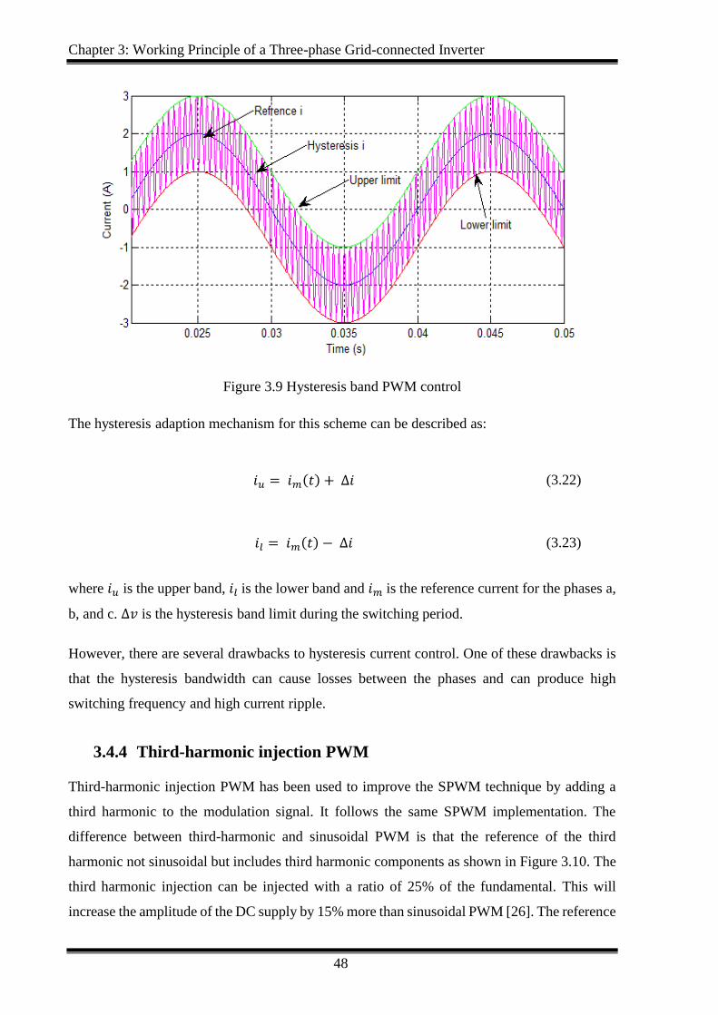
Chapter 3: Working Principle of a Three-phase Grid-connected Inverter
48
Figure 3.9 Hysteresis band PWM control
The hysteresis adaption mechanism for this scheme can be described as:
𝑖𝑢 = 𝑖𝑚(𝑡) + Δ𝑖 (3.22)
𝑖𝑙 = 𝑖𝑚(𝑡) − Δ𝑖 (3.23)
where 𝑖𝑢 is the upper band, 𝑖𝑙 is the lower band and 𝑖𝑚 is the reference current for the phases a,
b, and c. Δ𝑣 is the hysteresis band limit during the switching period.
However, there are several drawbacks to hysteresis current control. One of these drawbacks is
that the hysteresis bandwidth can cause losses between the phases and can produce high
switching frequency and high current ripple.
3.4.4 Third-harmonic injection PWM
Third-harmonic injection PWM has been used to improve the SPWM technique by adding a
third harmonic to the modulation signal. It follows the same SPWM implementation. The
difference between third-harmonic and sinusoidal PWM is that the reference of the third
harmonic not sinusoidal but includes third harmonic components as shown in Figure 3.10. The
third harmonic injection can be injected with a ratio of 25% of the fundamental. This will
increase the amplitude of the DC supply by 15% more than sinusoidal PWM [26]. The reference
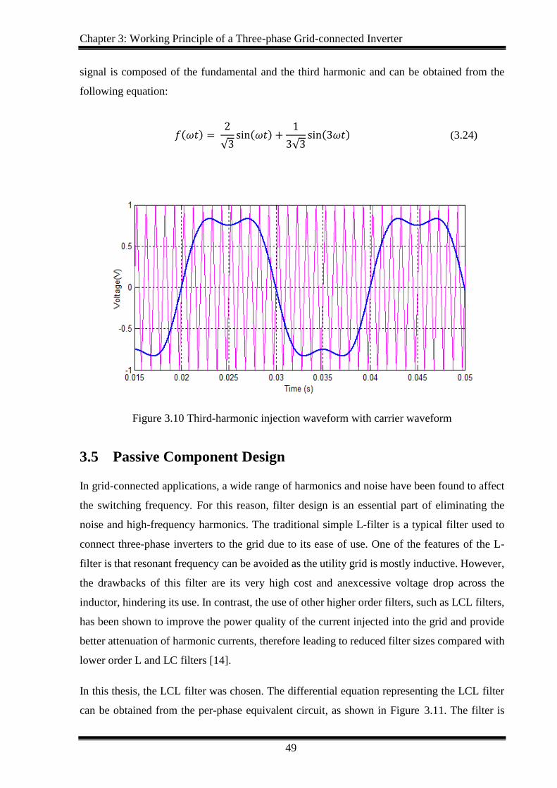
Chapter 3: Working Principle of a Three-phase Grid-connected Inverter
49
signal is composed of the fundamental and the third harmonic and can be obtained from the
following equation:
𝑓(𝜔𝑡) = 2
√3sin(𝜔𝑡) +
1
3√3sin(3𝜔𝑡) (3.24)
Figure 3.10 Third-harmonic injection waveform with carrier waveform
3.5 Passive Component Design
In grid-connected applications, a wide range of harmonics and noise have been found to affect
the switching frequency. For this reason, filter design is an essential part of eliminating the
noise and high-frequency harmonics. The traditional simple L-filter is a typical filter used to
connect three-phase inverters to the grid due to its ease of use. One of the features of the L-
filter is that resonant frequency can be avoided as the utility grid is mostly inductive. However,
the drawbacks of this filter are its very high cost and anexcessive voltage drop across the
inductor, hindering its use. In contrast, the use of other higher order filters, such as LCL filters,
has been shown to improve the power quality of the current injected into the grid and provide
better attenuation of harmonic currents, therefore leading to reduced filter sizes compared with
lower order L and LC filters [14].
In this thesis, the LCL filter was chosen. The differential equation representing the LCL filter
can be obtained from the per-phase equivalent circuit, as shown in Figure 3.11. The filter is
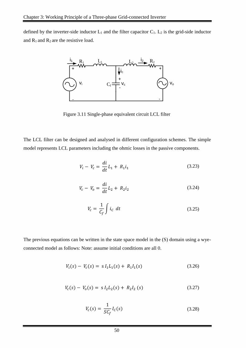
Chapter 3: Working Principle of a Three-phase Grid-connected Inverter
50
defined by the inverter-side inductor L1 and the filter capacitor C1. L2 is the grid-side inductor
and R1 and R2 are the resistive load.
Cf
L1 L2
+
-
i1 i2
vc
+
-
R1 R2
vo
+
-
vi
ic
Figure 3.11 Single-phase equivalent circuit LCL filter
The LCL filter can be designed and analysed in different configuration schemes. The simple
model represents LCL parameters including the ohmic losses in the passive components.
𝑉𝑖 − 𝑉𝑐 = 𝑑𝑖
𝑑𝑡𝐿1 + 𝑅1𝑖1 (3.23)
𝑉𝑐 − 𝑉𝑜 = 𝑑𝑖
𝑑𝑡𝐿2 + 𝑅2𝑖2 (3.24)
𝑉𝑐 = 1
𝐶𝑓∫𝑖𝐶 𝑑𝑡 (3.25)
The previous equations can be written in the state space model in the (S) domain using a wye-
connected model as follows: Note: assume initial conditions are all 0.
𝑉𝑖(𝑠) − 𝑉𝑐(𝑠) = s 𝐼1𝐿1(𝑠) + 𝑅1𝐼1(𝑠) (3.26)
𝑉𝑐(𝑠) − 𝑉𝑜(𝑠) = s 𝐼2𝐿2(𝑠) + 𝑅2𝐼2 (𝑠) (3.27)
𝑉𝑐(𝑠) = 1
𝑆𝐶𝑓𝐼𝐶(𝑠) (3.28)
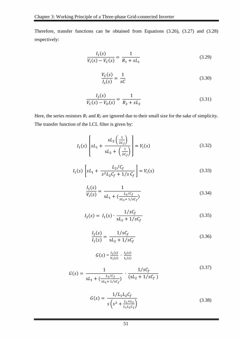
Chapter 3: Working Principle of a Three-phase Grid-connected Inverter
51
Therefore, transfer functions can be obtained from Equations (3.26), (3.27) and (3.28)
respectively:
𝐼1(𝑠)
𝑉𝑖(𝑠) − 𝑉𝐶(𝑠)=
1
𝑅1 + 𝑠𝐿1 (3.29)
𝑉𝐶(𝑠)
𝐼𝑠(𝑠)=
1
𝑠𝐶 (3.30)
𝐼2(𝑠)
𝑉𝐶(𝑠) − 𝑉𝑂(𝑠)=
1
𝑅2 + 𝑠𝐿2 (3.31)
Here, the series resistors R1 and R2 are ignored due to their small size for the sake of simplicity.
The transfer function of the LCL filter is given by:
𝐼1(𝑠) [𝑠𝐿1 + s𝐿2 (
1
𝑆𝐶𝑓)
s𝐿2 + ( 1
𝑆𝐶𝑓) ] = 𝑉𝑖(𝑠) (3.32)
𝐼1(𝑠) [𝑠𝐿1 + 𝐿2 𝐶𝑓⁄
𝑠2𝐿2𝐶𝑓 + 1 𝑠⁄ 𝐶𝑓 ] = 𝑉𝑖(𝑠) (3.33)
𝐼1(𝑠)
𝑉𝑖(𝑠)=
1
s𝐿1 + ( 𝐿2 𝐶𝑓⁄
𝑠𝐿2+ 1 𝑠⁄ 𝐶𝑓)
(3.34)
𝐼2(𝑠) = 𝐼1(𝑠) ∙ 1 𝑠𝐶𝑓⁄
s𝐿2 + 1 𝑠𝐶𝑓⁄ (3.35)
𝐼2(𝑠)
𝐼1(𝑠)=
1 𝑠𝐶𝑓⁄
s𝐿2 + 1 𝑠𝐶𝑓⁄ (3.36)
𝐺(𝑠) = 𝐼1(𝑠)
𝑉𝑖(𝑠) ∙
𝐼2(𝑠)
𝐼1(𝑠)
𝐺(𝑠) = 1
s𝐿1 + ( 𝐿2 𝐶𝑓⁄
𝑠𝐿2+ 1 𝑠⁄ 𝐶𝑓)
∙ 1 𝑠𝐶𝑓⁄
(s𝐿2 + 1 𝑠𝐶𝑓⁄ )
(3.37)
𝐺(𝑠) = 1 𝐿1𝐿2𝐶𝑓⁄
𝑠 (𝑠2 +𝐿1+𝐿2
𝐿1𝐿2𝐶𝑓) (3.38)
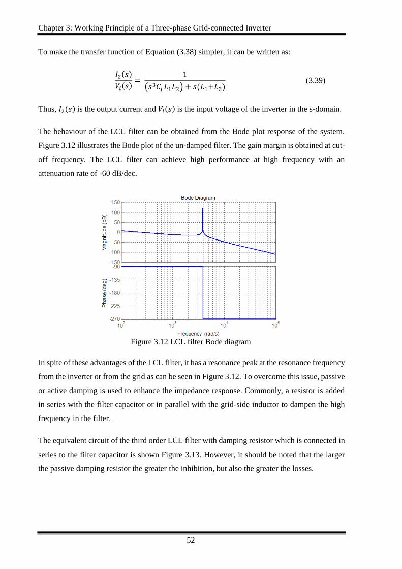
Chapter 3: Working Principle of a Three-phase Grid-connected Inverter
52
To make the transfer function of Equation (3.38) simpler, it can be written as:
𝐼2(𝑠)
𝑉𝑖(𝑠)=
1
(𝑠3𝐶𝑓𝐿1𝐿2) + 𝑠(𝐿1+𝐿2) (3.39)
Thus, 𝐼2(𝑠) is the output current and 𝑉𝑖(𝑠) is the input voltage of the inverter in the s-domain.
The behaviour of the LCL filter can be obtained from the Bode plot response of the system.
Figure 3.12 illustrates the Bode plot of the un-damped filter. The gain margin is obtained at cut-
off frequency. The LCL filter can achieve high performance at high frequency with an
attenuation rate of -60 dB/dec.
Figure 3.12 LCL filter Bode diagram
In spite of these advantages of the LCL filter, it has a resonance peak at the resonance frequency
from the inverter or from the grid as can be seen in Figure 3.12. To overcome this issue, passive
or active damping is used to enhance the impedance response. Commonly, a resistor is added
in series with the filter capacitor or in parallel with the grid-side inductor to dampen the high
frequency in the filter.
The equivalent circuit of the third order LCL filter with damping resistor which is connected in
series to the filter capacitor is shown Figure 3.13. However, it should be noted that the larger
the passive damping resistor the greater the inhibition, but also the greater the losses.
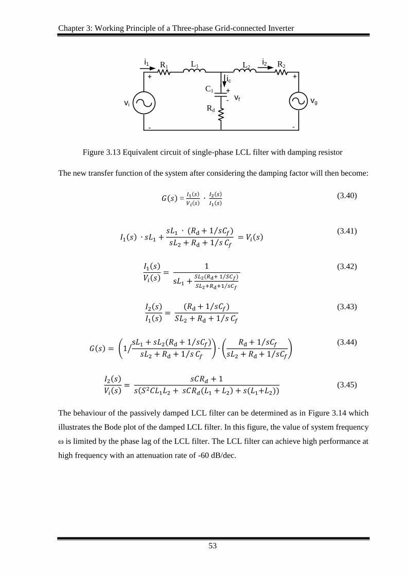
Chapter 3: Working Principle of a Three-phase Grid-connected Inverter
53
C1
L1 L2
+
vi
-
i1 i2
vf
+-
R1 R2
Rd
vg
+
-
ic
Figure 3.13 Equivalent circuit of single-phase LCL filter with damping resistor
The new transfer function of the system after considering the damping factor will then become:
𝐺(𝑠) = 𝐼1(𝑠)
𝑉𝑖(𝑠) ∙
𝐼2(𝑠)
𝐼1(𝑠) (3.40)
𝐼1(𝑠) ∙ 𝑠𝐿1 +𝑠𝐿1 ∙ (𝑅d + 1 𝑠𝐶𝑓)⁄
𝑠𝐿2 + 𝑅d + 1 𝑠⁄ 𝐶𝑓 = 𝑉𝑖(𝑠)
(3.41)
𝐼1(𝑠)
𝑉𝑖(𝑠)=
1
s𝐿1 +𝑆𝐿2(𝑅d+ 1 𝑆𝐶𝑓)⁄
𝑆𝐿2+𝑅d+1 𝑠⁄ 𝐶𝑓
(3.42)
𝐼2(𝑠)
𝐼1(𝑠)=
(𝑅d + 1 𝑠𝐶𝑓)⁄
𝑆𝐿2 + 𝑅d + 1 𝑠⁄ 𝐶𝑓
(3.43)
𝐺(𝑠) = (1s𝐿1 + 𝑠𝐿2(𝑅d + 1 𝑠𝐶𝑓)⁄
𝑠𝐿2 + 𝑅d + 1 𝑠⁄ 𝐶𝑓⁄ ) ∙ (
𝑅d + 1 𝑠𝐶𝑓⁄
𝑠𝐿2 + 𝑅d + 1 𝑠𝐶𝑓⁄)
(3.44)
𝐼2(𝑠)
𝑉𝑖(𝑠)=
𝑠𝐶𝑅𝑑 + 1
𝑠(𝑆2𝐶𝐿1𝐿2 + 𝑠𝐶𝑅𝑑(𝐿1 + 𝐿2) + 𝑠(𝐿1+𝐿2)) (3.45)
The behaviour of the passively damped LCL filter can be determined as in Figure 3.14 which
illustrates the Bode plot of the damped LCL filter. In this figure, the value of system frequency
ω is limited by the phase lag of the LCL filter. The LCL filter can achieve high performance at
high frequency with an attenuation rate of -60 dB/dec.
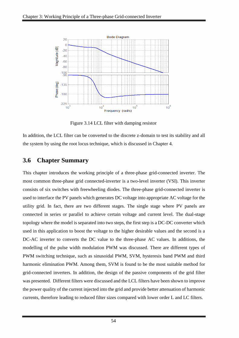
Chapter 3: Working Principle of a Three-phase Grid-connected Inverter
54
Figure 3.14 LCL filter with damping resistor
In addition, the LCL filter can be converted to the discrete z-domain to test its stability and all
the system by using the root locus technique, which is discussed in Chapter 4.
3.6 Chapter Summary
This chapter introduces the working principle of a three-phase grid-connected inverter. The
most common three-phase grid connected-inverter is a two-level inverter (VSI). This inverter
consists of six switches with freewheeling diodes. The three-phase grid-connected inverter is
used to interface the PV panels which generates DC voltage into appropriate AC voltage for the
utility grid. In fact, there are two different stages. The single stage where PV panels are
connected in series or parallel to achieve certain voltage and current level. The dual-stage
topology where the model is separated into two steps, the first step is a DC-DC converter which
used in this application to boost the voltage to the higher desirable values and the second is a
DC-AC inverter to converts the DC value to the three-phase AC values. In additions, the
modelling of the pulse width modulation PWM was discussed. There are different types of
PWM switching technique, such as sinusoidal PWM, SVM, hysteresis band PWM and third
harmonic elimination PWM. Among them, SVM is found to be the most suitable method for
grid-connected inverters. In addition, the design of the passive components of the grid filter
was presented. Different filters were discussed and the LCL filters have been shown to improve
the power quality of the current injected into the grid and provide better attenuation of harmonic
currents, therefore leading to reduced filter sizes compared with lower order L and LC filters.
Chapter 4: Grid Synchronization and Control of the Three-phase Gird-connected Inverter
55
Grid Synchronization and Control
of the Three-phase Gird-connected Inverter
4.1 Introduction
In this chapter, grid synchronization of the three-phase grid-connected inverter during normal
and abnormal grid conditions. In the unbalanced grid condition, the dynamic behaviour of the
system becomes progressively worse. AC components will cause power oscillation and
increased harmonic components in the system. Yet, this technique is not effectual if there is an
abnormal condition in the system, or if there should be any disruption in the network. Owing
to the negative-sequence terms, there will be oscillatory errors arising; consequently, the
dynamic behavior develops into something that is progressively worse. Based on the literature
review as discussed in chapter 1 and chapter 2, a method of decomposition is used in this thesis
to decompose the positive and negative sequence components.
The next section of this chapter investigates the main current control used for the three-phase
grid connected inverter. Current control is one of the most important challenges which needs to
be addressed. The main function of current control is to ensure that the reference signal is
followed by the measured signal. Many different current control techniques have been utilized
in order to achieve a better quality of the current waveform. In the three-phase system, current
control can be implemented in various ways such as Proportional Integral (PI) current control
in the synchronous rotating reference frame dq, and Proportional Resonance (PR) current
control in the stationary reference frame αβ.
4.2 Decomposition of the Symmetrical Components
Under abnormal grid conditions such as unsymmetrical voltage sags or swells, one or more of
the phase voltage drops or rises. As a result, the grid current and voltage lose their sinusoidal
and balanced appearance which makes the control system more challenging.
In this case, the negative sequence component is used to overcome the effect of the fault in the
injected current. Hence, it is necessary to use the method of decomposition to overcome
important issues regarding the operation of the three-phase inverter during unbalanced grid
conditions.
Chapter 4: Grid Synchronization and Control of the Three-phase Gird-connected Inverter
56
In normal grid conditions, the three-phase symmetrical component voltage has the same
frequency and amplitude with respect to the phase angle which is shifted in a clockwise
direction by 120° degrees. In general, a three-phase voltage can be written as:
𝑣𝑎( 𝑡) = √2𝑉𝑟𝑚𝑠 cos(𝜔𝑡) (4.1)
𝑣𝑏( 𝑡) = √2Vrmscos(𝜔𝑡 − 120°) (4.2)
𝑣𝑐( 𝑡) = √2𝑉𝑟𝑚𝑠 cos(𝜔𝑡 − 240°) (4.3)
Sometimes it is useful to present this information using the magnitude and phase angle as
presented in phase rotation as:
𝑣𝑎 = 𝑉𝑟𝑚𝑠 ∠0° (4.4)
𝑣𝑏 = 𝑉𝑟𝑚𝑠 ∠ − 120° (4.5)
𝑣𝑐 = 𝑉𝑟𝑚𝑠 ∠ − 240° (4.6)
Thus, the sum of three balanced voltages should be zero:
𝑣𝑎 + 𝑣𝑏 + 𝑣𝑐 = 𝑣𝑟𝑚𝑠( 1∠0° + 1∠ − 120° + 1∠120°) (4.7)
As a consequence, if there is any deviation from the above formula it will represent an abnormal
condition. This can happen when any difference in magnitude or deviation from the designated
phase angles is normally referred to as unbalanced. It must be noted that the difference between
the magnitude of the phase voltages is the most frequently occurring form of unbalance under
a normal mode of operation, and change in the phase normally occurs under faulty conditions.
To overcome this problem, using the symmetrical component method in the three-phase system
can convert the set of the three-phase voltages as well as the three-phase current into a linear
combination of the positive sequence components, the negative sequence, and the zero
sequence.
The symmetrical component can be written as
𝑣𝑎𝑏𝑐 = [
𝑣𝑎
𝑣𝑏
𝑣𝑐
] = ∑(
𝑛
𝑖=1
𝑣𝑎𝑏𝑐+ + 𝑣𝑎𝑏𝑐
− + 𝑣𝑎𝑏𝑐0) (4.8)
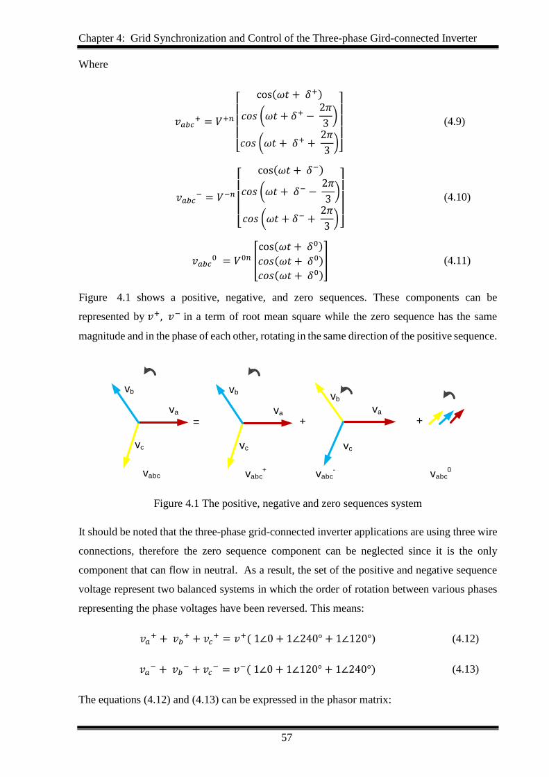
Chapter 4: Grid Synchronization and Control of the Three-phase Gird-connected Inverter
57
Where
𝑣𝑎𝑏𝑐+ = 𝑉+𝑛
[
cos(𝜔𝑡 + 𝛿+)
𝑐𝑜𝑠 (𝜔𝑡 + 𝛿+ − 2𝜋
3)
𝑐𝑜𝑠 (𝜔𝑡 + 𝛿+ + 2𝜋
3)]
(4.9)
𝑣𝑎𝑏𝑐− = 𝑉−𝑛
[
cos(𝜔𝑡 + 𝛿−)
𝑐𝑜𝑠 (𝜔𝑡 + 𝛿− − 2𝜋
3)
𝑐𝑜𝑠 (𝜔𝑡 + 𝛿− + 2𝜋
3)]
(4.10)
𝑣𝑎𝑏𝑐0 = 𝑉0𝑛 [
cos(𝜔𝑡 + 𝛿0)
𝑐𝑜𝑠(𝜔𝑡 + 𝛿0)
𝑐𝑜𝑠(𝜔𝑡 + 𝛿0)
] (4.11)
Figure 4.1 shows a positive, negative, and zero sequences. These components can be
represented by 𝑣+, 𝑣− in a term of root mean square while the zero sequence has the same
magnitude and in the phase of each other, rotating in the same direction of the positive sequence.
= ++
vabc0
vabc-
vabc+
va
vb
vc
va
vb
vc
vabc
va
vb
vc
Figure 4.1 The positive, negative and zero sequences system
It should be noted that the three-phase grid-connected inverter applications are using three wire
connections, therefore the zero sequence component can be neglected since it is the only
component that can flow in neutral. As a result, the set of the positive and negative sequence
voltage represent two balanced systems in which the order of rotation between various phases
representing the phase voltages have been reversed. This means:
𝑣𝑎+ + 𝑣𝑏
+ + 𝑣𝑐+ = 𝑣+( 1∠0 + 1∠240° + 1∠120°) (4.12)
𝑣𝑎− + 𝑣𝑏
− + 𝑣𝑐− = 𝑣−( 1∠0 + 1∠120° + 1∠240°) (4.13)
The equations (4.12) and (4.13) can be expressed in the phasor matrix:

Chapter 4: Grid Synchronization and Control of the Three-phase Gird-connected Inverter
58
[V±0]= [
V+
V−
V0
] = 1
3[1 α α2
1 α2 α1 1 1
] [
Va
Vb
Vc
] (4.14)
α is an operator defined as the reference for resulting symmetrical components which is α =
ej2π/3, or can be expressed in rectangular form as α = −1
2+ 𝑗
√3
2.
where 𝑗 = √−1 or 90° rotator.
Likewise, the inverse transformation of (4.14) is addressed to be
[Va
Vb
Vc
] = 1
3[1 1 1α2 α 1α α2 1
] [V+
V−
V0
] (4.15)
The voltage vector matrix of (4.15) can be expressed in the stationary α, β reference frame. The
voltage and the current are now decomposed to the positive sequence signal (PSS) and negative
sequence signal (NSS). Moreover, each of the two-phase voltages and two-phase currents can
be presented in
𝑣𝛼 = 𝑣𝛼+ + 𝑣𝛼
− , 𝑣𝛽 = 𝑣𝛽+ + 𝑣𝛽
− (4.16)
𝑖𝛼 = 𝑖𝛼+ + 𝑖𝛼
− , 𝑖𝛽 = 𝑖𝛽+ + 𝑖𝛽
− (4.17)
In the stationary reference frame, the component matrix can be reformulated from complex
operator α to signify the time delay in the period (𝑇0) by phase shift 90°. Figure 4.2 shows the
symmetrical component decomposition of a two-phase system in the stationary reference frame
α, β.
Part a) shows the relationship between the positions of α, β for both positive and negative
sequence components with respect to the phase angle 90°. Parts b) and c) show the
decomposition of α, β. The red vectors are the unbalanced components α, β of positive and
negative sequence components where the blue vectors are the result of both balance and
unbalance α, β.
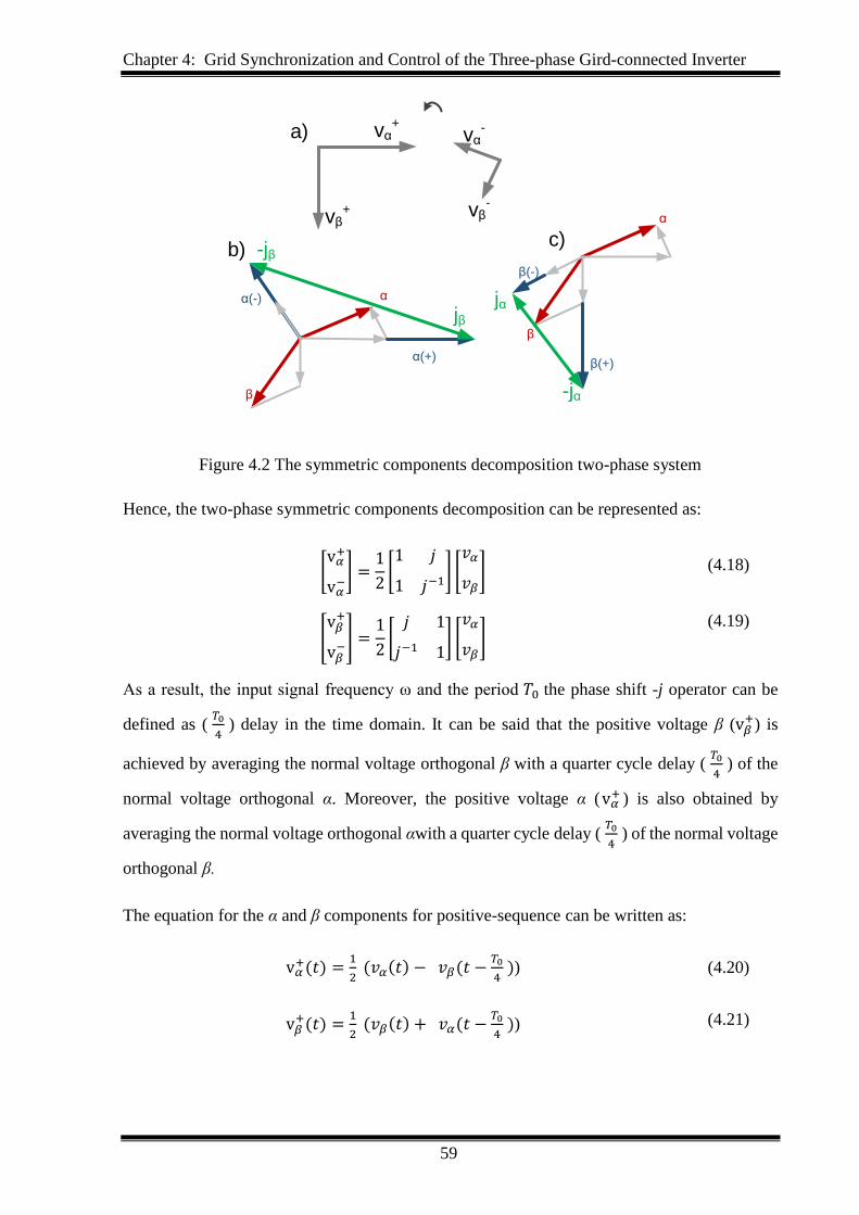
Chapter 4: Grid Synchronization and Control of the Three-phase Gird-connected Inverter
59
vα-vα
+
vβ+
a)
-jβ
jβ
α
β
jα
-jα
β(-)
β(+)α(+)
α(-)
c)b)
vβ-
α
β
Figure 4.2 The symmetric components decomposition two-phase system
Hence, the two-phase symmetric components decomposition can be represented as:
[v𝛼
+
v𝛼−] =
1
2[1 𝑗
1 𝑗−1] [
𝑣𝛼
𝑣𝛽] (4.18)
[v𝛽
+
v𝛽−] =
1
2[
𝑗 1
𝑗−1 1] [
𝑣𝛼
𝑣𝛽]
(4.19)
As a result, the input signal frequency ω and the period 𝑇0 the phase shift -j operator can be
defined as ( 𝑇0
4 ) delay in the time domain. It can be said that the positive voltage β (v𝛽
+) is
achieved by averaging the normal voltage orthogonal β with a quarter cycle delay ( 𝑇0
4 ) of the
normal voltage orthogonal α. Moreover, the positive voltage α (v𝛼+ ) is also obtained by
averaging the normal voltage orthogonal αwith a quarter cycle delay ( 𝑇0
4 ) of the normal voltage
orthogonal β.
The equation for the α and β components for positive-sequence can be written as:
v𝛼+(𝑡) =
1
2 (𝑣𝛼(𝑡) − 𝑣𝛽(𝑡 −
𝑇0
4 )) (4.20)
v𝛽+(𝑡) =
1
2 (𝑣𝛽(𝑡) + 𝑣𝛼(𝑡 −
𝑇0
4 )) (4.21)
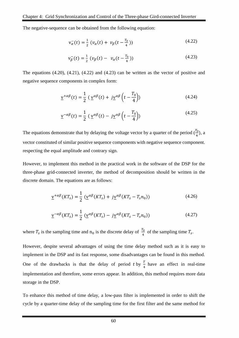
Chapter 4: Grid Synchronization and Control of the Three-phase Gird-connected Inverter
60
The negative-sequence can be obtained from the following equation:
v𝛼−(𝑡) =
1
2 (𝑣𝛼(𝑡) + 𝑣𝛽(𝑡 −
𝑇0
4 )) (4.22)
v𝛽−(𝑡) =
1
2 (𝑣𝛽(𝑡) − 𝑣𝛼(𝑡 −
𝑇0
4 )) (4.23)
The equations (4.20), (4.21), (4.22) and (4.23) can be written as the vector of positive and
negative sequence components in complex form:
v+𝛼𝛽(𝑡) =1
2 ( v𝛼𝛽(𝑡) + 𝑗v𝛼𝛽 (𝑡 −
𝑇0
4)) (4.24)
v−𝛼𝛽(𝑡) =1
2 ( v𝛼𝛽(𝑡) − 𝑗v𝛼𝛽 (𝑡 −
𝑇0
4))
(4.25)
The equations demonstrate that by delaying the voltage vector by a quarter of the period (𝑇0
4), a
vector constituted of similar positive sequence components with negative sequence component.
respecting the equal amplitude and contrary sign.
However, to implement this method in the practical work in the software of the DSP for the
three-phase grid-connected inverter, the method of decomposition should be written in the
discrete domain. The equations are as follows:
v+𝛼𝛽(𝐾𝑇𝑠) =1
2 (v𝛼𝛽(𝐾𝑇𝑠) + 𝑗v𝛼𝛽(𝐾𝑇𝑠 − 𝑇𝑠𝑛0)) (4.26)
v−𝛼𝛽(𝐾𝑇𝑠) =1
2 (v𝛼𝛽(𝐾𝑇𝑠) − 𝑗v𝛼𝛽(𝐾𝑇𝑠 − 𝑇𝑠𝑛0)) (4.27)
where 𝑇𝑠 is the sampling time and n0 is the discrete delay of 𝑇0
4 of the sampling time 𝑇𝑠.
However, despite several advantages of using the time delay method such as it is easy to
implement in the DSP and its fast response, some disadvantages can be found in this method.
One of the drawbacks is that the delay of period 𝑡 by 𝑇
4 have an effect in real-time
implementation and therefore, some errors appear. In addition, this method requires more data
storage in the DSP.
To enhance this method of time delay, a low-pass filter is implemented in order to shift the
cycle by a quarter-time delay of the sampling time for the first filter and the same method for
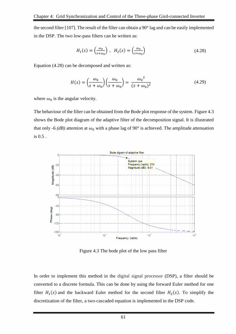
Chapter 4: Grid Synchronization and Control of the Three-phase Gird-connected Inverter
61
the second filter [107]. The result of the filter can obtain a 90° lag and can be easily implemented
in the DSP. The two low-pass filters can be written as:
𝐻1(𝑠) = (𝜔0
𝑠+𝜔0) , 𝐻2(𝑠) = (
𝜔0
𝑠+𝜔0) (4.28)
Equation (4.28) can be decomposed and written as:
𝐻(𝑠) = (𝜔0
𝑠 + 𝜔0) (
𝜔0
𝑠 + 𝜔0) =
𝜔02
(𝑠 + 𝜔0)2 (4.29)
where 𝜔0 is the angular velocity.
The behaviour of the filter can be obtained from the Bode plot response of the system. Figure 4.3
shows the Bode plot diagram of the adaptive filter of the decomposition signal. It is illustrated
that only -6 (dB) attention at 𝜔0 with a phase lag of 90° is achieved. The amplitude attenuation
is 0.5 .
Figure 4.3 The bode plot of the low pass filter
In order to implement this method in the digital signal processor (DSP), a filter should be
converted to a discrete formula. This can be done by using the forward Euler method for one
filter 𝐻1(𝑠) and the backward Euler method for the second filter 𝐻2(𝑠). To simplify the
discretization of the filter, a two-cascaded equation is implemented in the DSP code.
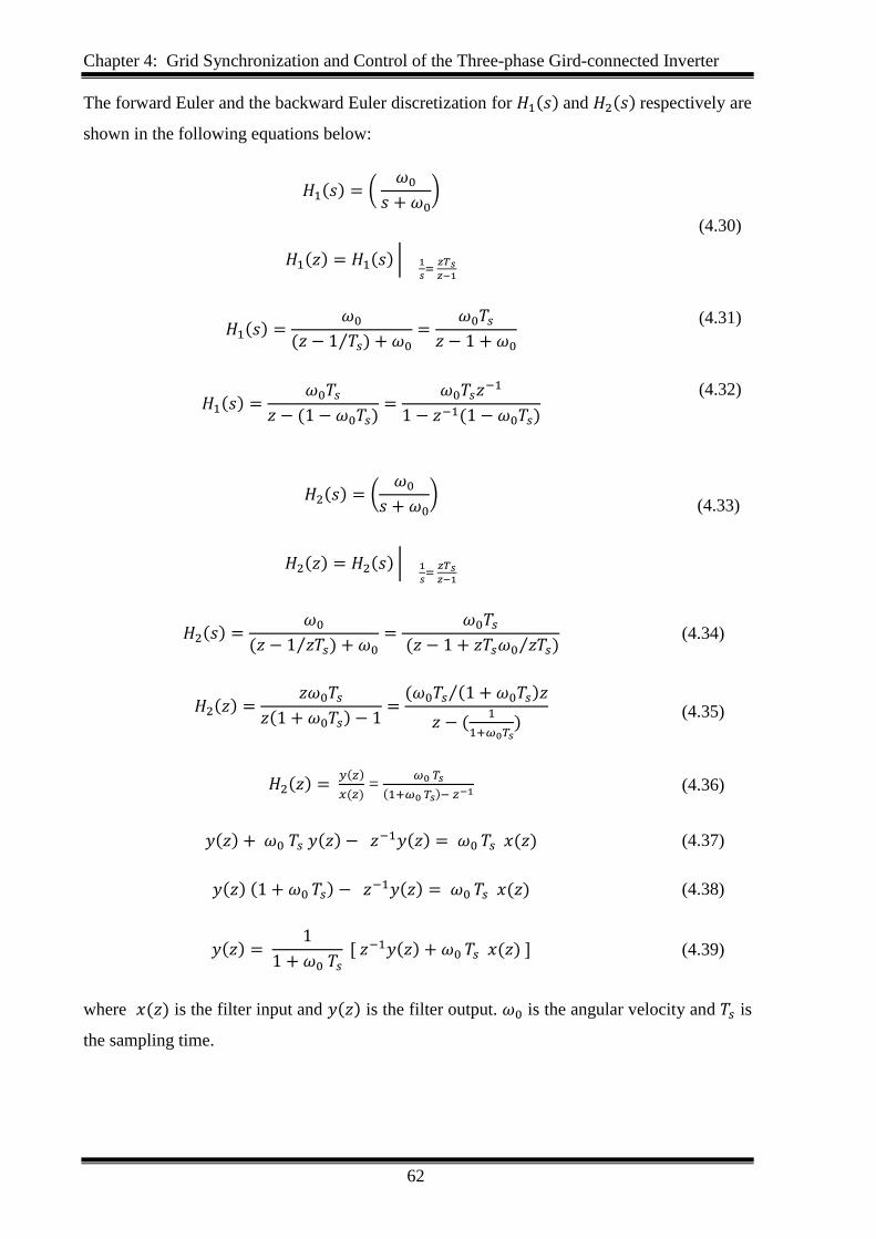
Chapter 4: Grid Synchronization and Control of the Three-phase Gird-connected Inverter
62
The forward Euler and the backward Euler discretization for 𝐻1(𝑠) and 𝐻2(𝑠) respectively are
shown in the following equations below:
𝐻1(𝑠) = ( 𝜔0
𝑠 + 𝜔0)
𝐻1(𝑧) = 𝐻1(𝑠) | 1
𝑠=
𝑧𝑇𝑠𝑧−1
(4.30)
𝐻1(𝑠) =𝜔0
(𝑧 − 1 𝑇𝑠⁄ ) + 𝜔0=
𝜔0𝑇𝑠
𝑧 − 1 + 𝜔0
(4.31)
𝐻1(𝑠) =𝜔0𝑇𝑠
𝑧 − (1 − 𝜔0𝑇𝑠)=
𝜔0𝑇𝑠𝑧−1
1 − 𝑧−1(1 − 𝜔0𝑇𝑠)
(4.32)
𝐻2(𝑠) = (𝜔0
𝑠 + 𝜔0)
𝐻2(𝑧) = 𝐻2(𝑠) | 1
𝑠=
𝑧𝑇𝑠𝑧−1
(4.33)
𝐻2(𝑠) =𝜔0
(𝑧 − 1 𝑧𝑇𝑠⁄ ) + 𝜔0=
𝜔0𝑇𝑠
(𝑧 − 1 + 𝑧𝑇𝑠𝜔0 𝑧𝑇𝑠⁄ ) (4.34)
𝐻2(𝑧) =𝑧𝜔0𝑇𝑠
𝑧(1 + 𝜔0𝑇𝑠) − 1=
(𝜔0𝑇𝑠 (1 + 𝜔0𝑇𝑠)𝑧⁄
𝑧 − (1
1+𝜔0𝑇𝑠)
(4.35)
𝐻2(𝑧) = 𝑦(𝑧)
𝑥(𝑧) =
𝜔0 𝑇𝑠
(1+𝜔0 𝑇𝑠)− 𝑧−1 (4.36)
𝑦(𝑧) + 𝜔0 𝑇𝑠 𝑦(𝑧) − 𝑧−1𝑦(𝑧) = 𝜔0 𝑇𝑠 𝑥(𝑧) (4.37)
𝑦(𝑧) (1 + 𝜔0 𝑇𝑠) − 𝑧−1𝑦(𝑧) = 𝜔0 𝑇𝑠 𝑥(𝑧) (4.38)
𝑦(𝑧) = 1
1 + 𝜔0 𝑇𝑠 [ 𝑧−1𝑦(𝑧) + 𝜔0 𝑇𝑠 𝑥(𝑧) ] (4.39)
where 𝑥(𝑧) is the filter input and 𝑦(𝑧) is the filter output. 𝜔0 is the angular velocity and 𝑇𝑠 is
the sampling time.
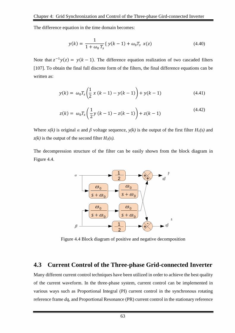
Chapter 4: Grid Synchronization and Control of the Three-phase Gird-connected Inverter
63
The difference equation in the time domain becomes:
𝑦(𝑘) = 1
1 + 𝜔0 𝑇𝑠 𝑦(𝑘 − 1) + 𝜔0𝑇𝑠 𝑥(𝑧) (4.40)
Note that 𝑧−1𝑦(𝑧) = 𝑦(𝑘 − 1). The difference equation realization of two cascaded filters
[107]. To obtain the final full discrete form of the filters, the final difference equations can be
written as:
𝑦(𝑘) = 𝜔0𝑇𝑠 (1
2 𝑥 (𝑘 − 1) − 𝑦(𝑘 − 1)) + 𝑦(𝑘 − 1) (4.41)
𝑧(𝑘) = 𝜔0𝑇𝑠 ( 1
2𝑦 (𝑘 − 1) − 𝑧(𝑘 − 1)) + 𝑧(𝑘 − 1)
(4.42)
Where x(k) is original α and β voltage sequence, y(k) is the output of the first filter H1(s) and
z(k) is the output of the second filter H2(s).
The decompression structure of the filter can be easily shown from the block diagram in
Figure 4.4.
0
0
s
p
0
0
s 0
0
s
+-
++
n
1
2
1
2
0
0
s
Figure 4.4 Block diagram of positive and negative decomposition
4.3 Current Control of the Three-phase Grid-connected Inverter
Many different current control techniques have been utilized in order to achieve the best quality
of the current waveform. In the three-phase system, current control can be implemented in
various ways such as Proportional Integral (PI) current control in the synchronous rotating
reference frame dq, and Proportional Resonance (PR) current control in the stationary reference
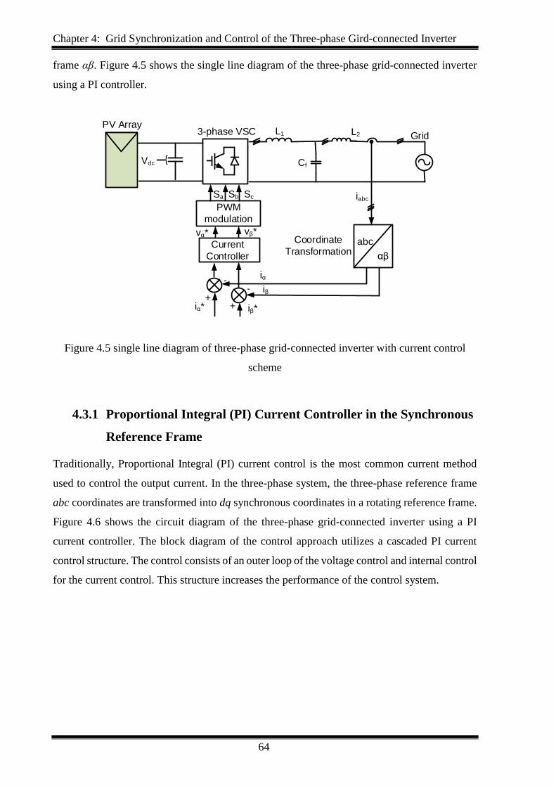
Chapter 4: Grid Synchronization and Control of the Three-phase Gird-connected Inverter
64
frame αβ. Figure 4.5 shows the single line diagram of the three-phase grid-connected inverter
using a PI controller.
PWM
modulation
Sa Sb Sc
abc
Vdc
αβ
iabc
PV Array3-phase VSC L1
vα* vβ*
Cf
L2
iβ*iα*
Current
Controller
++
--
iα
iβ
Grid
Coordinate
Transformation
Figure 4.5 single line diagram of three-phase grid-connected inverter with current control
scheme
4.3.1 Proportional Integral (PI) Current Controller in the Synchronous
Reference Frame
Traditionally, Proportional Integral (PI) current control is the most common current method
used to control the output current. In the three-phase system, the three-phase reference frame
abc coordinates are transformed into dq synchronous coordinates in a rotating reference frame.
Figure 4.6 shows the circuit diagram of the three-phase grid-connected inverter using a PI
current controller. The block diagram of the control approach utilizes a cascaded PI current
control structure. The control consists of an outer loop of the voltage control and internal control
for the current control. This structure increases the performance of the control system.
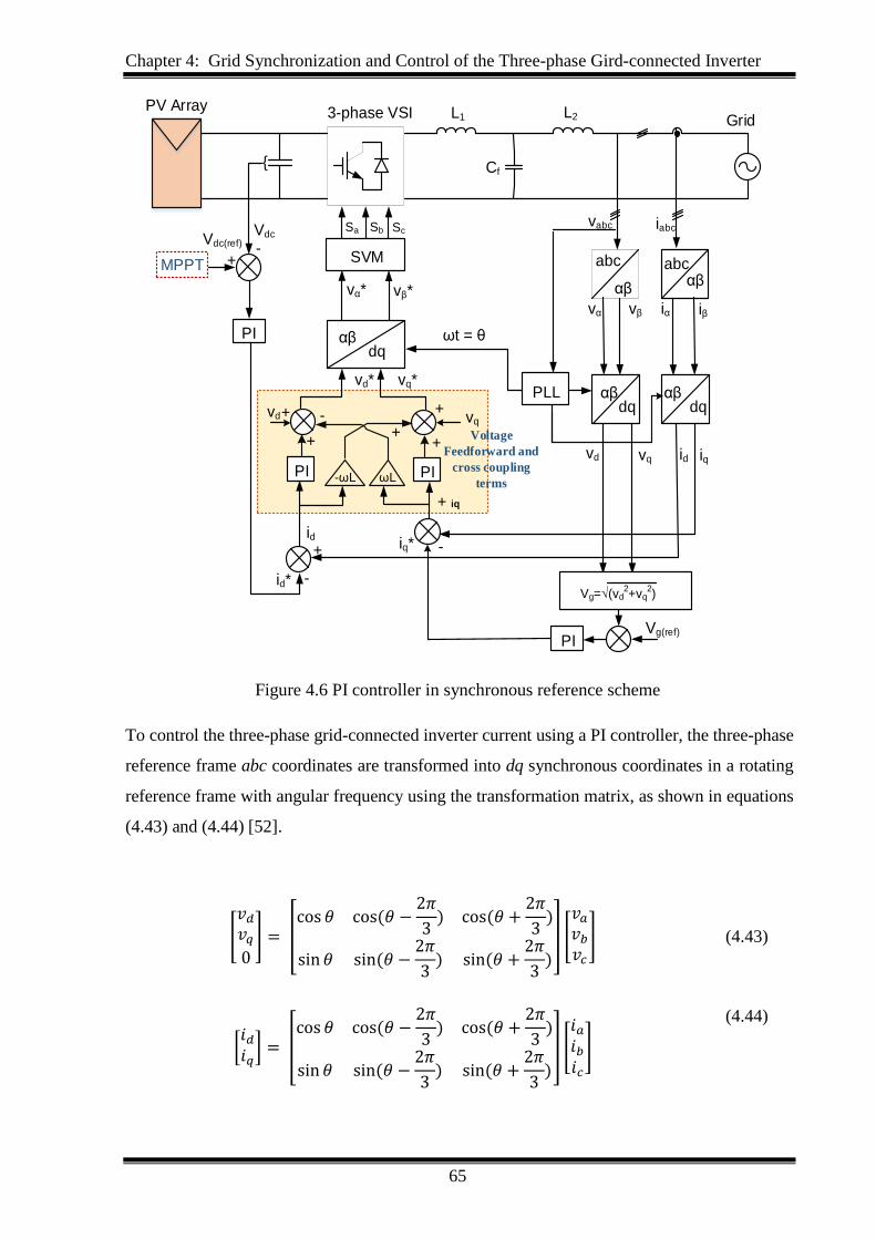
Chapter 4: Grid Synchronization and Control of the Three-phase Gird-connected Inverter
65
SVM
Sa Sb Sc
αβdq
PI
abc abc
PLL
vα iα iβvβ
Vdc
-
PI
Vdc(ref)
ωt = θ
+
αβαβ
iabcvabc
vd* vq*
vα* vβ*
PV Array 3-phase VSI L1 L2
Cf
Grid
PI
Vg=√(vd2+vq
2)
Vg(ref)
ωL
αβαβdqdq
iq*
iq
id iq
id
id* -
-
+
+
+
++ -
++
vqvd
vqvd
-ωLPI
Voltage
Feedforward and
cross coupling
terms
MPPT
Figure 4.6 PI controller in synchronous reference scheme
To control the three-phase grid-connected inverter current using a PI controller, the three-phase
reference frame abc coordinates are transformed into dq synchronous coordinates in a rotating
reference frame with angular frequency using the transformation matrix, as shown in equations
(4.43) and (4.44) [52].
[
𝑣𝑑
𝑣𝑞
0] = [
cos 𝜃 cos(𝜃 −2𝜋
3) cos(𝜃 +
2𝜋
3)
sin 𝜃 sin(𝜃 −2𝜋
3) sin(𝜃 +
2𝜋
3)
] [
𝑣𝑎
𝑣𝑏
𝑣𝑐
] (4.43)
[𝑖𝑑𝑖𝑞
] = [cos 𝜃 cos(𝜃 −
2𝜋
3) cos(𝜃 +
2𝜋
3)
sin 𝜃 sin(𝜃 −2𝜋
3) sin(𝜃 +
2𝜋
3)
] [𝑖𝑎𝑖𝑏𝑖𝑐
]
(4.44)
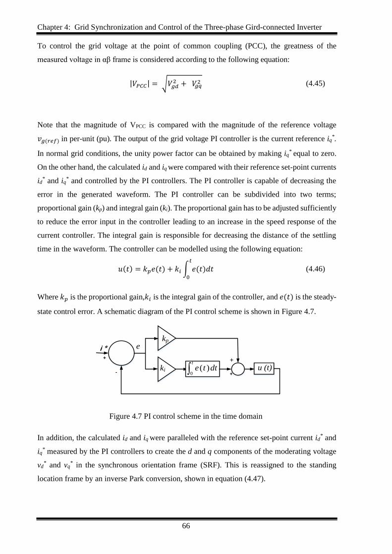
Chapter 4: Grid Synchronization and Control of the Three-phase Gird-connected Inverter
66
To control the grid voltage at the point of common coupling (PCC), the greatness of the
measured voltage in αβ frame is considered according to the following equation:
|𝑉𝑃𝐶𝐶| = √𝑉𝑔𝑑2 + 𝑉𝑔𝑞
2 (4.45)
Note that the magnitude of VPCC is compared with the magnitude of the reference voltage
𝑣𝑔(𝑟𝑒𝑓) in per-unit (pu). The output of the grid voltage PI controller is the current reference iq*.
In normal grid conditions, the unity power factor can be obtained by making iq* equal to zero.
On the other hand, the calculated id and iq were compared with their reference set-point currents
id* and iq
* and controlled by the PI controllers. The PI controller is capable of decreasing the
error in the generated waveform. The PI controller can be subdivided into two terms;
proportional gain (kp) and integral gain (ki). The proportional gain has to be adjusted sufficiently
to reduce the error input in the controller leading to an increase in the speed response of the
current controller. The integral gain is responsible for decreasing the distance of the settling
time in the waveform. The controller can be modelled using the following equation:
𝑢(𝑡) = 𝑘𝑝𝑒(𝑡) + 𝑘𝑖 ∫ 𝑒(𝑡)𝑑𝑡𝑡
0
(4.46)
Where 𝑘𝑝 is the proportional gain,𝑘𝑖 is the integral gain of the controller, and 𝑒(𝑡) is the steady-
state control error. A schematic diagram of the PI control scheme is shown in Figure 4.7.
kpkp
+
+
kp
i *
t
dtte0
)(-
+
ki
e
u (t)
Figure 4.7 PI control scheme in the time domain
In addition, the calculated id and iq were paralleled with the reference set-point current id* and
iq* measured by the PI controllers to create the d and q components of the moderating voltage
vd* and vq
* in the synchronous orientation frame (SRF). This is reassigned to the standing
location frame by an inverse Park conversion, shown in equation (4.47).
Chapter 4: Grid Synchronization and Control of the Three-phase Gird-connected Inverter
67
[𝑣𝑑
∗
𝑣𝑞∗] = [
cos 𝜃 − sin 𝜃sin 𝜃 cos 𝜃
] [𝑣𝛼
∗
𝑣𝛽∗] (4.47)
The grid voltage feed-forward procedures are occasionally related in grid-connected purposes to
relieve some of the weight on the PI controller itself thus developing the response of the AC
tracking system [143]. The current in the synchronous reference frame can be described from
the single-phase equivalent circuit in d and q components as follows:
[𝑣𝑑
∗
𝑣𝑞∗] = 𝐿
𝑑
𝑑𝑡[𝑖𝑑𝑖𝑞
] + 𝐿𝜔 [−𝑖𝑞𝑖𝑑
] + 𝑅 [𝑖𝑑𝑖𝑞
] + [𝑒𝑑
𝑒𝑞] (4.48)
where 𝑣𝑑∗ and 𝑣𝑞
∗ are the inverter voltages in d and q components, 𝑒𝑑 and 𝑒𝑞 are the grid voltages,
R and L are the total resistors and inductance of the grid filter.
From equation (4.42), there is a clear cross-coupling of the currents in the d-axis and q-axis.
Stereotypically, such cross-coupling can make unwelcome disruption which disturbs the
dynamic retort of the system as each axis concurrently impacts upon the other [144]. Due to this,
a voltage feed-forward de-coupling strategy is added, as shown in Figure 4.6 [39].
On the other hand, the PI controller can be described in the state space transfer and is defined as
follows [53]:
𝐺𝑝𝑖(𝑠) = 𝑘𝑝 +𝑘𝑖
𝑠 (4.49)
Where, 𝑘𝑝 is the proportional gain and 𝑘𝑖 is the integral gain of the controller.
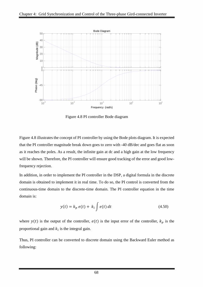
Chapter 4: Grid Synchronization and Control of the Three-phase Gird-connected Inverter
68
Figure 4.8 PI controller Bode diagram
Figure 4.8 illustrates the concept of PI controller by using the Bode plots diagram. It is expected
that the PI controller magnitude break down goes to zero with -40 dB/dec and goes flat as soon
as it reaches the poles. As a result, the infinite gain at dc and a high gain at the low frequency
will be shown. Therefore, the PI controller will ensure good tracking of the error and good low-
frequency rejection.
In addition, in order to implement the PI controller in the DSP, a digital formula in the discrete
domain is obtained to implement it in real time. To do so, the PI control is converted from the
continuous-time domain to the discrete-time domain. The PI controller equation in the time
domain is:
𝑦(𝑡) = 𝑘𝑝 𝑒(𝑡) + 𝑘𝑖 ∫𝑒(𝑡) 𝑑𝑡 (4.50)
where 𝑦(𝑡) is the output of the controller, 𝑒(𝑡) is the input error of the controller, 𝑘𝑝 is the
proportional gain and 𝑘𝑖 is the integral gain.
Thus, PI controller can be converted to discrete domain using the Backward Euler method as
following:
0
10
20
30
40
50M
agnitu
de (
dB
)
10-3
10-2
10-1
100
101
-90
-45
0
Phase (
deg)
Bode Diagram
Frequency (rad/s)

Chapter 4: Grid Synchronization and Control of the Three-phase Gird-connected Inverter
69
1
𝑠=
𝑇𝑠
1 − 𝑧−1
(4.51)
𝑠 =1 − 𝑧−1
𝑇𝑠
The PI controller in discrete form is as follows:
𝑑𝑦
𝑑𝑡= 𝑘𝑝 (
𝑑. 𝑒
𝑑𝑡+
𝑘𝑖
𝑘𝑝𝑒) (4.52)
𝑦(𝐾) − 𝑦(𝐾 − 1)
𝑇𝑠= 𝑘𝑝 (
𝑒(𝑘) − 𝑒(𝑘 − 1)
𝑇𝑠+
𝑘𝑖
𝑘𝑝𝑒(𝑘)) (4.53)
𝑦(𝐾) − 𝑦(𝐾 − 1) = 𝑘𝑝 (𝑒(𝑘) − 𝑒(𝑘 − 1) +𝑘𝑖
𝑘𝑝𝑇𝑠. 𝑒(𝑘)) (4.54)
𝑦(𝐾) = 𝑦(𝐾 − 1) + 𝑘𝑝 (𝑒(𝑘) [1 +𝑘𝑖
𝑘𝑝𝑇𝑠] − 𝑒(𝑘 − 1)) (4.55)
4.3.2 Stability of Proportional Integral (PI) Current Controller
In order to test the stability of the system and obtain the impact of the PI controller in the system,
the Bode plot and root locus of the closed loop of the PI controller are obtained. First of all, the
whole system will be converted into a transfer function to test the stability of the system. The
control block diagram is shown in Figure 4.9. The open loop and closed loop system transfer
functions are addressed. The control system has used the Bode plot for the open loop and root
locus for the closed loop. The root locus is one of the methods used to design a closed loop
control system.
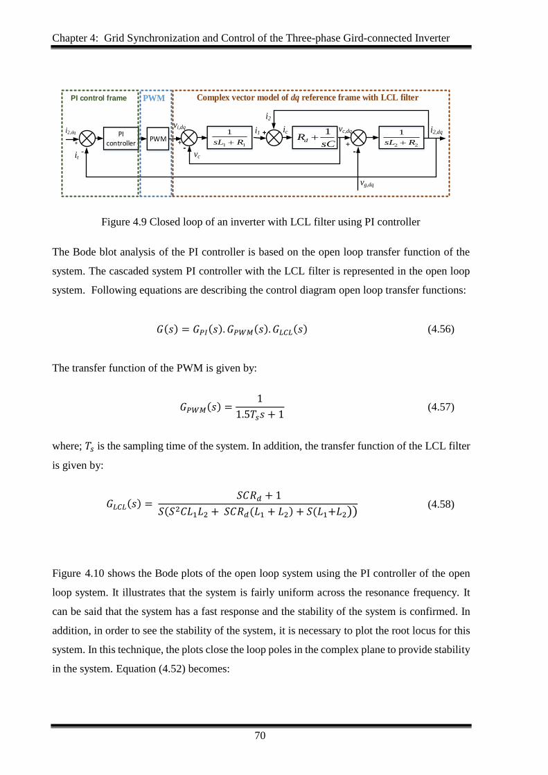
Chapter 4: Grid Synchronization and Control of the Three-phase Gird-connected Inverter
70
-+-
+
vg,dq
22
1
RsL sCRd
1
ici1i2,dq
vc
+PWMPI
controller+
it-
i2,dq
11
1
RsL
vi,dq vc,dq
i2
Complex vector model of dq reference frame with LCL filter PWM PI control frame
Figure 4.9 Closed loop of an inverter with LCL filter using PI controller
The Bode blot analysis of the PI controller is based on the open loop transfer function of the
system. The cascaded system PI controller with the LCL filter is represented in the open loop
system. Following equations are describing the control diagram open loop transfer functions:
𝐺(𝑠) = 𝐺𝑃𝐼(𝑠). 𝐺𝑃𝑊𝑀(𝑠). 𝐺𝐿𝐶𝐿(𝑠) (4.56)
The transfer function of the PWM is given by:
𝐺𝑃𝑊𝑀(𝑠) =1
1.5𝑇𝑠𝑠 + 1 (4.57)
where; 𝑇𝑠 is the sampling time of the system. In addition, the transfer function of the LCL filter
is given by:
𝐺𝐿𝐶𝐿(𝑠) = 𝑆𝐶𝑅𝑑 + 1
𝑆(𝑆2𝐶𝐿1𝐿2 + 𝑆𝐶𝑅𝑑(𝐿1 + 𝐿2) + 𝑆(𝐿1+𝐿2)) (4.58)
Figure 4.10 shows the Bode plots of the open loop system using the PI controller of the open
loop system. It illustrates that the system is fairly uniform across the resonance frequency. It
can be said that the system has a fast response and the stability of the system is confirmed. In
addition, in order to see the stability of the system, it is necessary to plot the root locus for this
system. In this technique, the plots close the loop poles in the complex plane to provide stability
in the system. Equation (4.52) becomes:
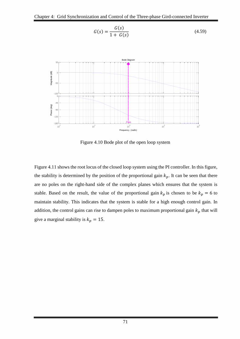
Chapter 4: Grid Synchronization and Control of the Three-phase Gird-connected Inverter
71
𝐺(𝑠) =𝐺(𝑠)
1 + 𝐺(𝑠) (4.59)
Figure 4.10 Bode plot of the open loop system
Figure 4.11 shows the root locus of the closed loop system using the PI controller. In this figure,
the stability is determined by the position of the proportional gain 𝑘𝑝. It can be seen that there
are no poles on the right-hand side of the complex planes which ensures that the system is
stable. Based on the result, the value of the proportional gain 𝑘𝑝 is chosen to be 𝑘𝑝 = 6 to
maintain stability. This indicates that the system is stable for a high enough control gain. In
addition, the control gains can rise to dampen poles to maximum proportional gain 𝑘𝑝 that will
give a marginal stability is 𝑘𝑝 = 15.
-100
-50
0
50
Magnitu
de (
dB
)
102
103
104
105
106
-180
-135
-90
-45
0
Phase (
deg)
Bode Diagram
Frequency (rad/s)
Fres
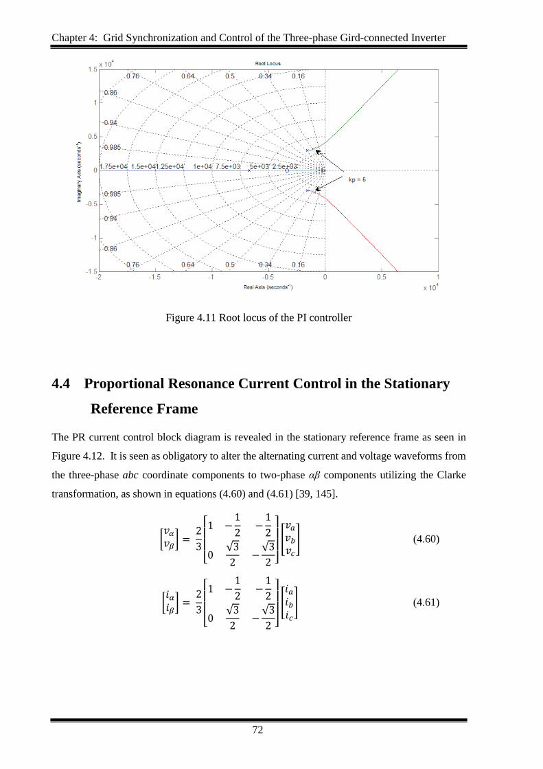
Chapter 4: Grid Synchronization and Control of the Three-phase Gird-connected Inverter
72
Figure 4.11 Root locus of the PI controller
4.4 Proportional Resonance Current Control in the Stationary
Reference Frame
The PR current control block diagram is revealed in the stationary reference frame as seen in
Figure 4.12. It is seen as obligatory to alter the alternating current and voltage waveforms from
the three-phase abc coordinate components to two-phase αβ components utilizing the Clarke
transformation, as shown in equations (4.60) and (4.61) [39, 145].
[𝑣𝛼
𝑣𝛽] =
2
3[ 1 −
1
2−
1
2
0√3
2−
√3
2 ]
[
𝑣𝑎
𝑣𝑏
𝑣𝑐
] (4.60)
[𝑖𝛼𝑖𝛽
] = 2
3[ 1 −
1
2−
1
2
0√3
2−
√3
2 ]
[𝑖𝑎𝑖𝑏𝑖𝑐
] (4.61)
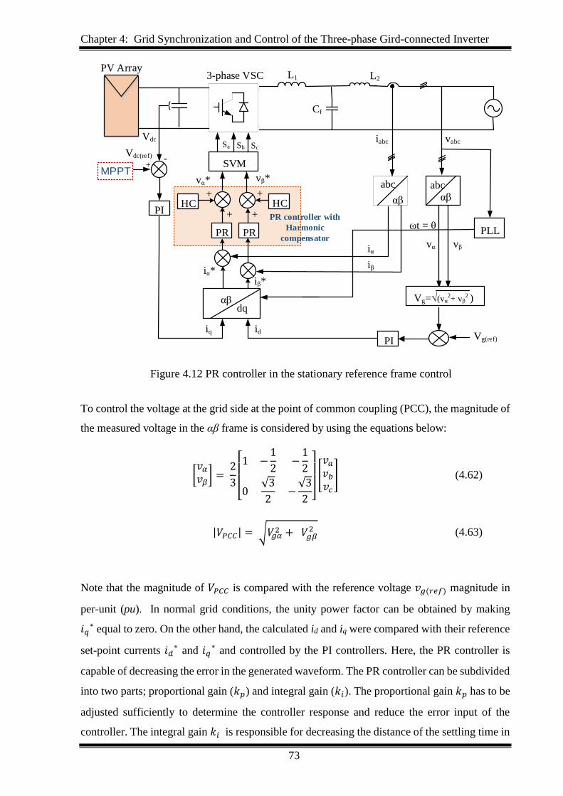
Chapter 4: Grid Synchronization and Control of the Three-phase Gird-connected Inverter
73
SVM
Sa Sb Sc
PR PR
abc abc
PLL
vαiα
iβ
vβ
Vdc
-
PI
Vdc(ref)
+
ωt = θ
+
αβαβ
iabc vabc
PV Array3-phase VSC L1
PI Vg(ref)
αβdq
HC+ +
++
vα* vβ*
Cf
L2
iβ*iα*
Vg=√(vα2+ vβ
2 )
idiq
MPPT
HC
PR controller with
Harmonic
compensator
Figure 4.12 PR controller in the stationary reference frame control
To control the voltage at the grid side at the point of common coupling (PCC), the magnitude of
the measured voltage in the αβ frame is considered by using the equations below:
[𝑣𝛼
𝑣𝛽] =
2
3[ 1 −
1
2−
1
2
0√3
2−
√3
2 ]
[
𝑣𝑎
𝑣𝑏
𝑣𝑐
] (4.62)
|𝑉𝑃𝐶𝐶| = √𝑉𝑔𝛼2 + 𝑉𝑔𝛽
2 (4.63)
Note that the magnitude of 𝑉𝑃𝐶𝐶 is compared with the reference voltage 𝑣𝑔(𝑟𝑒𝑓) magnitude in
per-unit (pu). In normal grid conditions, the unity power factor can be obtained by making
𝑖𝑞∗ equal to zero. On the other hand, the calculated id and iq were compared with their reference
set-point currents 𝑖𝑑∗ and 𝑖𝑞
∗ and controlled by the PI controllers. Here, the PR controller is
capable of decreasing the error in the generated waveform. The PR controller can be subdivided
into two parts; proportional gain (𝑘𝑝) and integral gain (𝑘𝑖). The proportional gain 𝑘𝑝 has to be
adjusted sufficiently to determine the controller response and reduce the error input of the
controller. The integral gain 𝑘𝑖 is responsible for decreasing the distance of the settling time in

Chapter 4: Grid Synchronization and Control of the Three-phase Gird-connected Inverter
74
the waveform and controlling the bandwidth around it. The controller can be modelled using
the following equation:
𝑢(𝑡) = 𝐾𝑝𝑒(𝑡) + 𝐾𝑖 cosω𝑡 ∫ 𝑒(𝑡)𝑑𝑡𝑡
0
(4.64)
where 𝐾𝑝 is the proportional gain, 𝐾𝑖 is the integral gain of the controller, and 𝑒(𝑡) is the steady-
state control error. The transfer function of the ideal PR controller is given by the equation:
𝐺𝑃𝑅(s) = 𝐾𝑝 + 𝐾𝑖
𝑠
(𝑠2 + ω𝑜2)
(4.65)
where ω𝑜 is the resonant (line) frequency. Due to the high noticeable advance at the fundamental
frequency 𝜔, a balanced state error can be characteristically detached via the PR controller.
A chart diagram of the PR control scheme is presented in Figure 4.13.
kpkp
ω2
y U++
+
-
kp
kii
Gf (s)
ɛi *
1/s
1/s
a ω
Figure 4.13 Control Diagram of PR controller implementation
Nevertheless, to circumvent the problem of obtaining an infinite gain at the resonant frequency,
a non-ideal PR controller which is given in the following equation can be used instead:
𝐺𝑃𝑅(s) = 𝐾𝑝 + 𝐾𝑖
2𝜔𝑐𝑠
(𝑠2 + 2𝜔𝑐𝑠+ω𝑜2)
(4.66)
where kp is the proportional gain, ki is the integral gain of the controller, 𝜔0 is the resonance
frequency, and 𝜔𝑐 is the cut off frequency and 𝜔𝑐 ≪ 𝜔0.
Figure 4.14 shows the Bode plots diagram for PR controller in both causes ideal and non-ideal.
It clearly shows that the non-ideal PR controller has less gain in the narrow frequency over the
entirety of the resonance frequency compared with an ideal one.
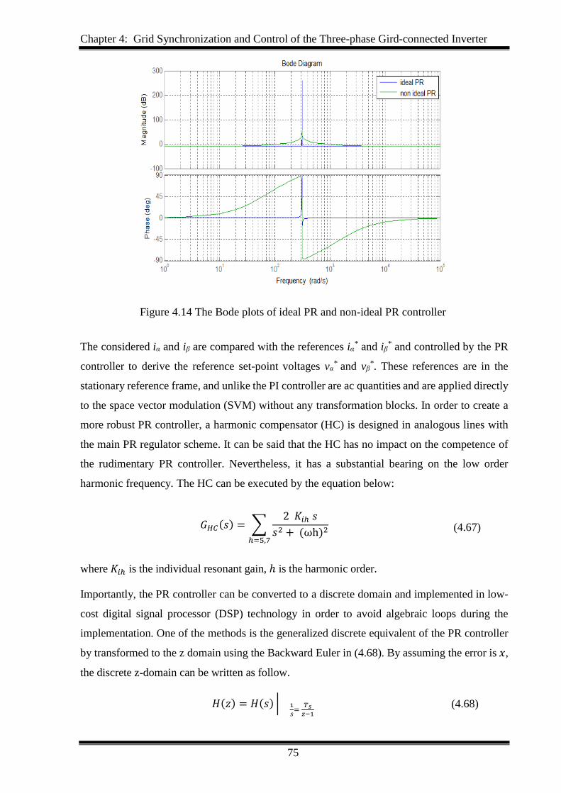
Chapter 4: Grid Synchronization and Control of the Three-phase Gird-connected Inverter
75
Figure 4.14 The Bode plots of ideal PR and non-ideal PR controller
The considered iα and iβ are compared with the references iα* and iβ
* and controlled by the PR
controller to derive the reference set-point voltages vα* and vβ
*. These references are in the
stationary reference frame, and unlike the PI controller are ac quantities and are applied directly
to the space vector modulation (SVM) without any transformation blocks. In order to create a
more robust PR controller, a harmonic compensator (HC) is designed in analogous lines with
the main PR regulator scheme. It can be said that the HC has no impact on the competence of
the rudimentary PR controller. Nevertheless, it has a substantial bearing on the low order
harmonic frequency. The HC can be executed by the equation below:
𝐺𝐻𝐶(𝑠) = ∑2 𝐾𝑖ℎ 𝑠
𝑠2 + (ωh)2
ℎ=5,7
(4.67)
where 𝐾𝑖ℎ is the individual resonant gain, ℎ is the harmonic order.
Importantly, the PR controller can be converted to a discrete domain and implemented in low-
cost digital signal processor (DSP) technology in order to avoid algebraic loops during the
implementation. One of the methods is the generalized discrete equivalent of the PR controller
by transformed to the z domain using the Backward Euler in (4.68). By assuming the error is 𝑥,
the discrete z-domain can be written as follow.
𝐻(𝑧) = 𝐻(𝑠) | 1
𝑠=
𝑇𝑠𝑧−1
(4.68)
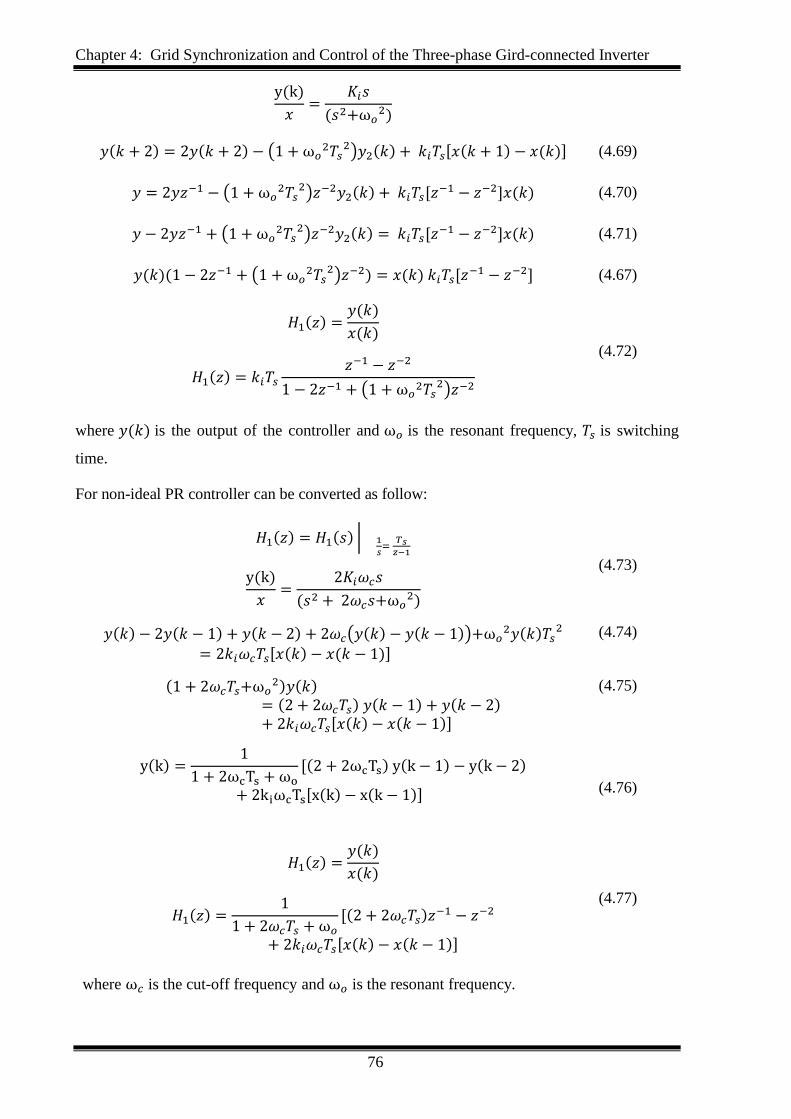
Chapter 4: Grid Synchronization and Control of the Three-phase Gird-connected Inverter
76
y(k)
𝑥=
𝐾𝑖𝑠
(𝑠2+ω𝑜2)
𝑦(𝑘 + 2) = 2𝑦(𝑘 + 2) − (1 + ω𝑜2𝑇𝑠
2)𝑦2(𝑘) + 𝑘𝑖𝑇𝑠[𝑥(𝑘 + 1) − 𝑥(𝑘)] (4.69)
𝑦 = 2𝑦𝑧−1 − (1 + ω𝑜2𝑇𝑠
2)𝑧−2𝑦2(𝑘) + 𝑘𝑖𝑇𝑠[𝑧−1 − 𝑧−2]𝑥(𝑘) (4.70)
𝑦 − 2𝑦𝑧−1 + (1 + ω𝑜2𝑇𝑠
2)𝑧−2𝑦2(𝑘) = 𝑘𝑖𝑇𝑠[𝑧−1 − 𝑧−2]𝑥(𝑘) (4.71)
𝑦(𝑘)(1 − 2𝑧−1 + (1 + ω𝑜2𝑇𝑠
2)𝑧−2) = 𝑥(𝑘) 𝑘𝑖𝑇𝑠[𝑧−1 − 𝑧−2] (4.67)
𝐻1(𝑧) =𝑦(𝑘)
𝑥(𝑘)
𝐻1(𝑧) = 𝑘𝑖𝑇𝑠
𝑧−1 − 𝑧−2
1 − 2𝑧−1 + (1 + ω𝑜2𝑇𝑠
2)𝑧−2
(4.72)
where 𝑦(𝑘) is the output of the controller and ω𝑜 is the resonant frequency, 𝑇𝑠 is switching
time.
For non-ideal PR controller can be converted as follow:
𝐻1(𝑧) = 𝐻1(𝑠) | 1
𝑠=
𝑇𝑠𝑧−1
y(k)
𝑥=
2𝐾𝑖𝜔𝑐𝑠
(𝑠2 + 2𝜔𝑐𝑠+ω𝑜2)
(4.73)
𝑦(𝑘) − 2𝑦(𝑘 − 1) + 𝑦(𝑘 − 2) + 2𝜔𝑐(𝑦(𝑘) − 𝑦(𝑘 − 1))+ω𝑜2𝑦(𝑘)𝑇𝑠
2
= 2𝑘𝑖𝜔𝑐𝑇𝑠[𝑥(𝑘) − 𝑥(𝑘 − 1)]
(4.74)
(1 + 2𝜔𝑐𝑇𝑠+ω𝑜2)𝑦(𝑘)
= (2 + 2𝜔𝑐𝑇𝑠) 𝑦(𝑘 − 1) + 𝑦(𝑘 − 2)+ 2𝑘𝑖𝜔𝑐𝑇𝑠[𝑥(𝑘) − 𝑥(𝑘 − 1)]
(4.75)
y(k) =1
1 + 2ωcTs + ωo[(2 + 2ωcTs) y(k − 1) − y(k − 2)
+ 2kiωcTs[x(k) − x(k − 1)]
(4.76)
𝐻1(𝑧) =𝑦(𝑘)
𝑥(𝑘)
𝐻1(𝑧) =1
1 + 2𝜔𝑐𝑇𝑠 + ω𝑜[(2 + 2𝜔𝑐𝑇𝑠)𝑧
−1 − 𝑧−2
+ 2𝑘𝑖𝜔𝑐𝑇𝑠[𝑥(𝑘) − 𝑥(𝑘 − 1)]
(4.77)
where ω𝑐 is the cut-off frequency and ω𝑜 is the resonant frequency.
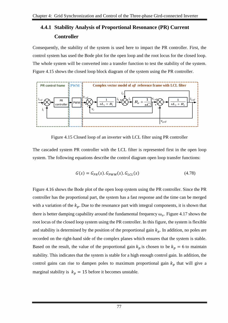
Chapter 4: Grid Synchronization and Control of the Three-phase Gird-connected Inverter
77
4.4.1 Stability Analysis of Proportional Resonance (PR) Current
Controller
Consequently, the stability of the system is used here to impact the PR controller. First, the
control system has used the Bode plot for the open loop and the root locus for the closed loop.
The whole system will be converted into a transfer function to test the stability of the system.
Figure 4.15 shows the closed loop block diagram of the system using the PR controller.
-+-
+
vg,αβ
22
1
RsL sCRd
1
ici1i2,αβ
vc
+PWMPR
controller+
it-
i2,αβ
11
1
RsL
vi,αβ vc,αβ
i2
Complex vector model of αβ reference frame with LCL filter PWM PR control frame
Figure 4.15 Closed loop of an inverter with LCL filter using PR controller
The cascaded system PR controller with the LCL filter is represented first in the open loop
system. The following equations describe the control diagram open loop transfer functions:
𝐺(𝑠) = 𝐺𝑃𝑅(𝑠). 𝐺𝑃𝑊𝑀(𝑠). 𝐺𝐿𝐶𝐿(𝑠) (4.78)
Figure 4.16 shows the Bode plot of the open loop system using the PR controller. Since the PR
controller has the proportional part, the system has a fast response and the time can be merged
with a variation of the 𝑘𝑝. Due to the resonance part with integral components, it is shown that
there is better damping capability around the fundamental frequency ω𝑜. Figure 4.17 shows the
root locus of the closed loop system using the PR controller. In this figure, the system is flexible
and stability is determined by the position of the proportional gain 𝑘𝑝. In addition, no poles are
recorded on the right-hand side of the complex planes which ensures that the system is stable.
Based on the result, the value of the proportional gain 𝑘𝑝 is chosen to be 𝑘𝑝 = 6 to maintain
stability. This indicates that the system is stable for a high enough control gain. In addition, the
control gains can rise to dampen poles to maximum proportional gain 𝑘𝑝 that will give a
marginal stability is 𝑘𝑝 = 15 before it becomes unstable.
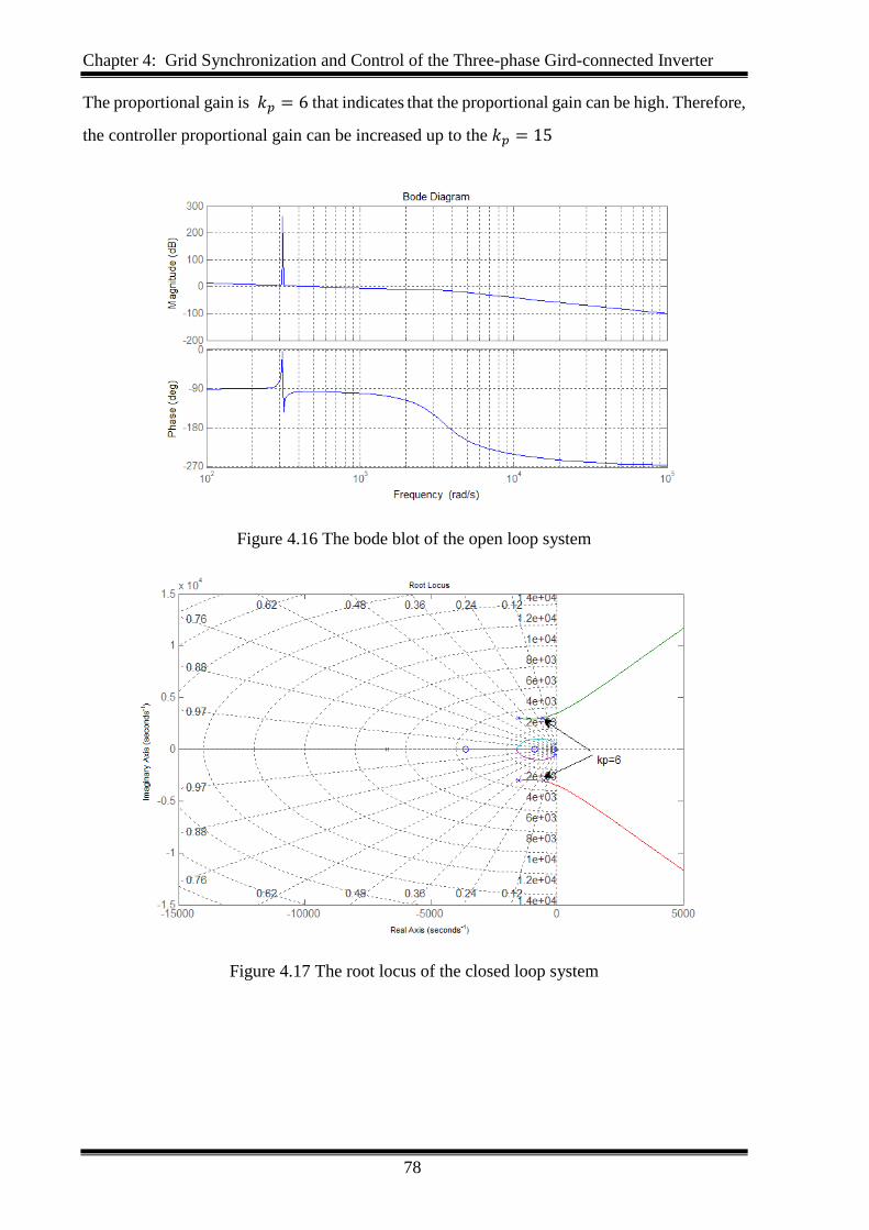
Chapter 4: Grid Synchronization and Control of the Three-phase Gird-connected Inverter
78
The proportional gain is 𝑘𝑝 = 6 that indicates that the proportional gain can be high. Therefore,
the controller proportional gain can be increased up to the 𝑘𝑝 = 15
Figure 4.16 The bode blot of the open loop system
Figure 4.17 The root locus of the closed loop system
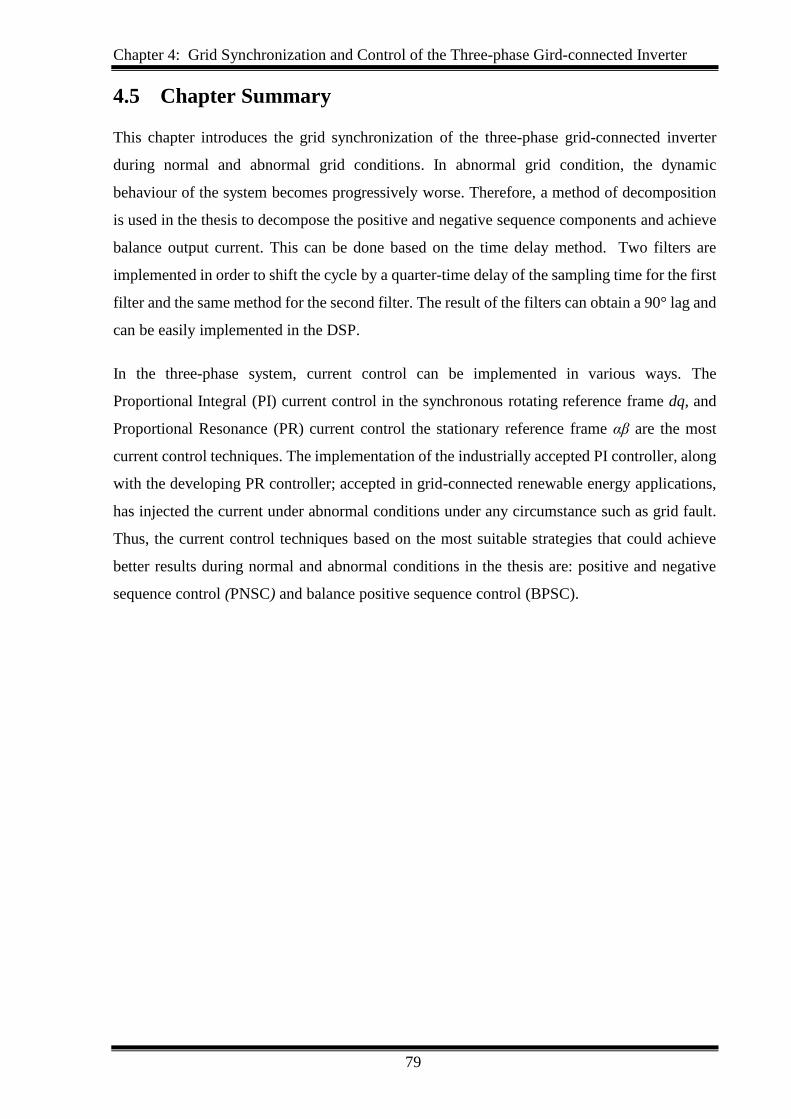
Chapter 4: Grid Synchronization and Control of the Three-phase Gird-connected Inverter
79
4.5 Chapter Summary
This chapter introduces the grid synchronization of the three-phase grid-connected inverter
during normal and abnormal grid conditions. In abnormal grid condition, the dynamic
behaviour of the system becomes progressively worse. Therefore, a method of decomposition
is used in the thesis to decompose the positive and negative sequence components and achieve
balance output current. This can be done based on the time delay method. Two filters are
implemented in order to shift the cycle by a quarter-time delay of the sampling time for the first
filter and the same method for the second filter. The result of the filters can obtain a 90° lag and
can be easily implemented in the DSP.
In the three-phase system, current control can be implemented in various ways. The
Proportional Integral (PI) current control in the synchronous rotating reference frame dq, and
Proportional Resonance (PR) current control the stationary reference frame αβ are the most
current control techniques. The implementation of the industrially accepted PI controller, along
with the developing PR controller; accepted in grid-connected renewable energy applications,
has injected the current under abnormal conditions under any circumstance such as grid fault.
Thus, the current control techniques based on the most suitable strategies that could achieve
better results during normal and abnormal conditions in the thesis are: positive and negative
sequence control (PNSC) and balance positive sequence control (BPSC).
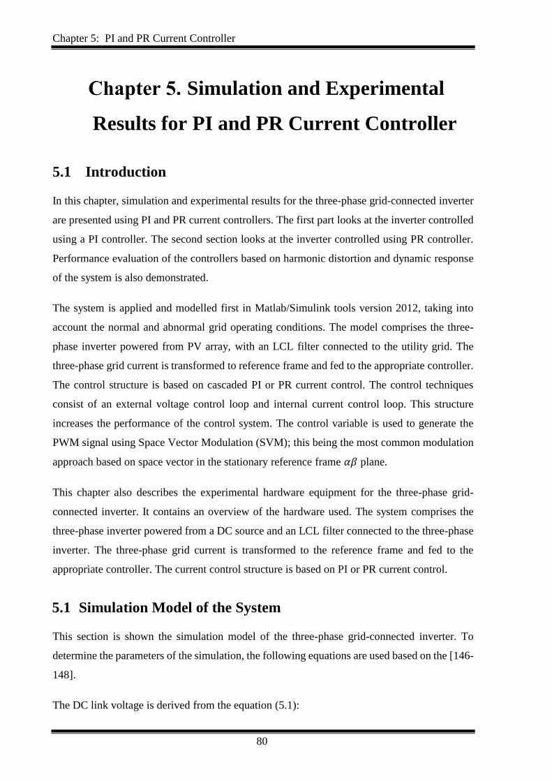
Chapter 5: PI and PR Current Controller
80
Simulation and Experimental
Results for PI and PR Current Controller
5.1 Introduction
In this chapter, simulation and experimental results for the three-phase grid-connected inverter
are presented using PI and PR current controllers. The first part looks at the inverter controlled
using a PI controller. The second section looks at the inverter controlled using PR controller.
Performance evaluation of the controllers based on harmonic distortion and dynamic response
of the system is also demonstrated.
The system is applied and modelled first in Matlab/Simulink tools version 2012, taking into
account the normal and abnormal grid operating conditions. The model comprises the three-
phase inverter powered from PV array, with an LCL filter connected to the utility grid. The
three-phase grid current is transformed to reference frame and fed to the appropriate controller.
The control structure is based on cascaded PI or PR current control. The control techniques
consist of an external voltage control loop and internal current control loop. This structure
increases the performance of the control system. The control variable is used to generate the
PWM signal using Space Vector Modulation (SVM); this being the most common modulation
approach based on space vector in the stationary reference frame 𝛼𝛽 plane.
This chapter also describes the experimental hardware equipment for the three-phase grid-
connected inverter. It contains an overview of the hardware used. The system comprises the
three-phase inverter powered from a DC source and an LCL filter connected to the three-phase
inverter. The three-phase grid current is transformed to the reference frame and fed to the
appropriate controller. The current control structure is based on PI or PR current control.
5.1 Simulation Model of the System
This section is shown the simulation model of the three-phase grid-connected inverter. To
determine the parameters of the simulation, the following equations are used based on the [146-
148].
The DC link voltage is derived from the equation (5.1):

Chapter 5: PI and PR Current Controller
81
𝑉𝑑𝑐 =2 √2
𝑚𝑖 √3 𝑉𝐿
(5.1)
where 𝑉𝑑𝑐 is the dc link voltage, 𝑉𝐿 is the line voltage, 𝑚𝑖 is the modulation index.
The inductances and capacitance values of the LCL filter are calculated from the base values
using (5.2) and (5.30) respectively.
𝑍𝑏 =𝑉𝐿𝐿
2
𝑃 (5.2)
𝐶𝑏 =1
𝑍𝑏𝜔𝑛
(5.3)
where 𝑉𝐿𝐿 is the line to line voltage, 𝑃 is the active power, 𝑍𝑏 is the base impedance, 𝐶𝑏 is the
base capacitance and 𝜔𝑛 is the grid frequency.
The filter capacitor is a relation between the allowable fraction of the reactive power at rated
voltage and current expressed as:
𝐶𝑓 = 𝑥1𝐶𝑏 (5.4)
where 𝐶𝑓 is the filter capacitor, 𝑥1 is the allowable fraction and has been chosen to be 5%.
To design the inverter-side inductor (L1), which L1 is chosen to reduce the ripple in the current.
The allowable current ripple should be considered as the percentage of the inverter current and
is given by:
∆𝑖𝐿 =𝑉𝑑
2𝐿1𝑓𝑠 (5.5)
where ∆𝑖𝐿 is the allowable per-unit ripple in the line current and 𝑓𝑠 is the switching frequency.
The value of ∆𝑖𝐿 is chosen to be equal to 10% of the line current
∆ 𝑖𝐿 = 𝑥2 𝑖𝐿 (5.6)
where 𝑖𝐿 is the output inverter current, 𝑥2 is allowable current ripple and has been chosen to be
25%.

Chapter 5: PI and PR Current Controller
82
The inverter-side inductor L1 is given by:
𝐿1 = 𝑉𝑑𝑐
(8 ∗ 𝑓𝑠 ∗ ∆𝑖𝐿) (5.7)
where 𝑓𝑠 is the switching frequency. In addition, the grid-side inductor L2 is designated as a
segment of the inverter-side inductance which is accountable for the diminution of the majority
of the switching ripple. Consequently, 𝐿2 is a function of the inverter-side inductor L1 and can
be calculated as:
𝐿2 = 𝑥3 𝐿1 (5.8)
Where 𝑥3 is the ratio index between the inductance at the inverter-side and grid-side.
𝐶𝑓 = 𝑥𝐶𝑏 (5.9)
where 𝐶𝑏 is the base filter capacitor.
The resonant frequency of the LCL filter can be calculated as:
𝑓𝑟𝑒𝑠 = 1
2𝜋√
𝐿1 + 𝐿2
𝐿1𝐿2𝐶𝑓 (5.10)
This resonant frequency is chosen to be at least 10 times the line frequency but less than half of
the switching frequency [150].
From the above equations, the nominal operating parameters used in the simulation model are
listed in Table 5.1.
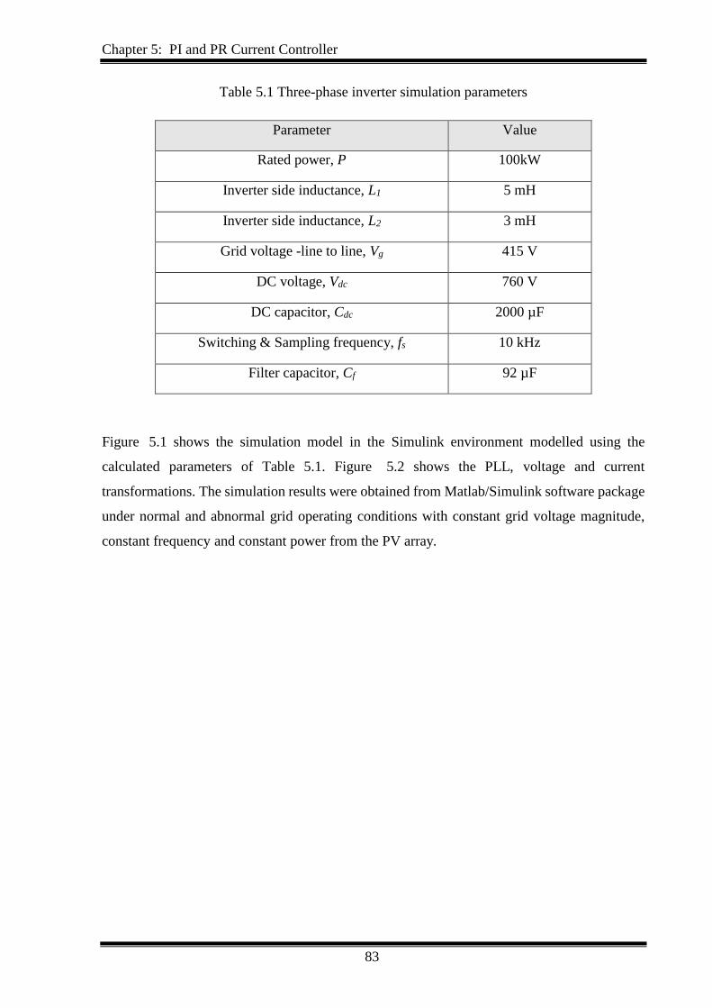
Chapter 5: PI and PR Current Controller
83
Table 5.1 Three-phase inverter simulation parameters
Parameter Value
Rated power, P 100kW
Inverter side inductance, L1 5 mH
Inverter side inductance, L2 3 mH
Grid voltage -line to line, Vg 415 V
DC voltage, Vdc 760 V
DC capacitor, Cdc 2000 µF
Switching & Sampling frequency, fs 10 kHz
Filter capacitor, Cf 92 µF
Figure 5.1 shows the simulation model in the Simulink environment modelled using the
calculated parameters of Table 5.1. Figure 5.2 shows the PLL, voltage and current
transformations. The simulation results were obtained from Matlab/Simulink software package
under normal and abnormal grid operating conditions with constant grid voltage magnitude,
constant frequency and constant power from the PV array.
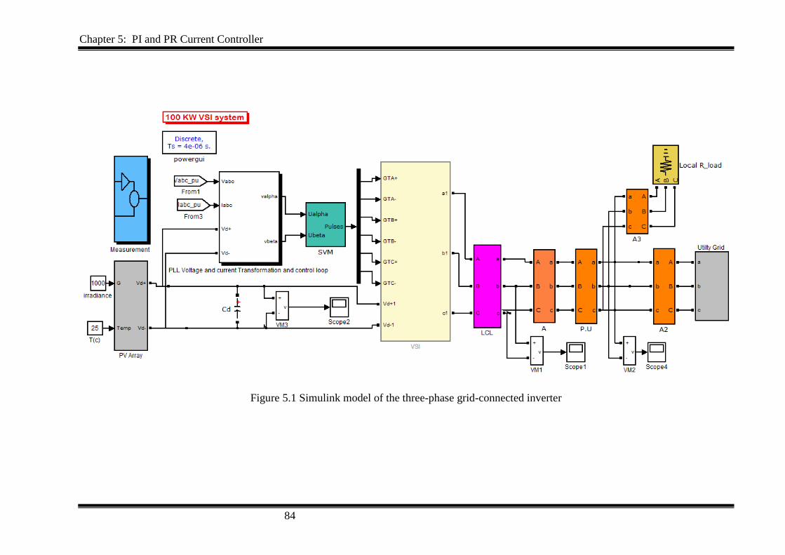
Chapter 5: PI and PR Current Controller
84
Figure 5.1 Simulink model of the three-phase grid-connected inverter
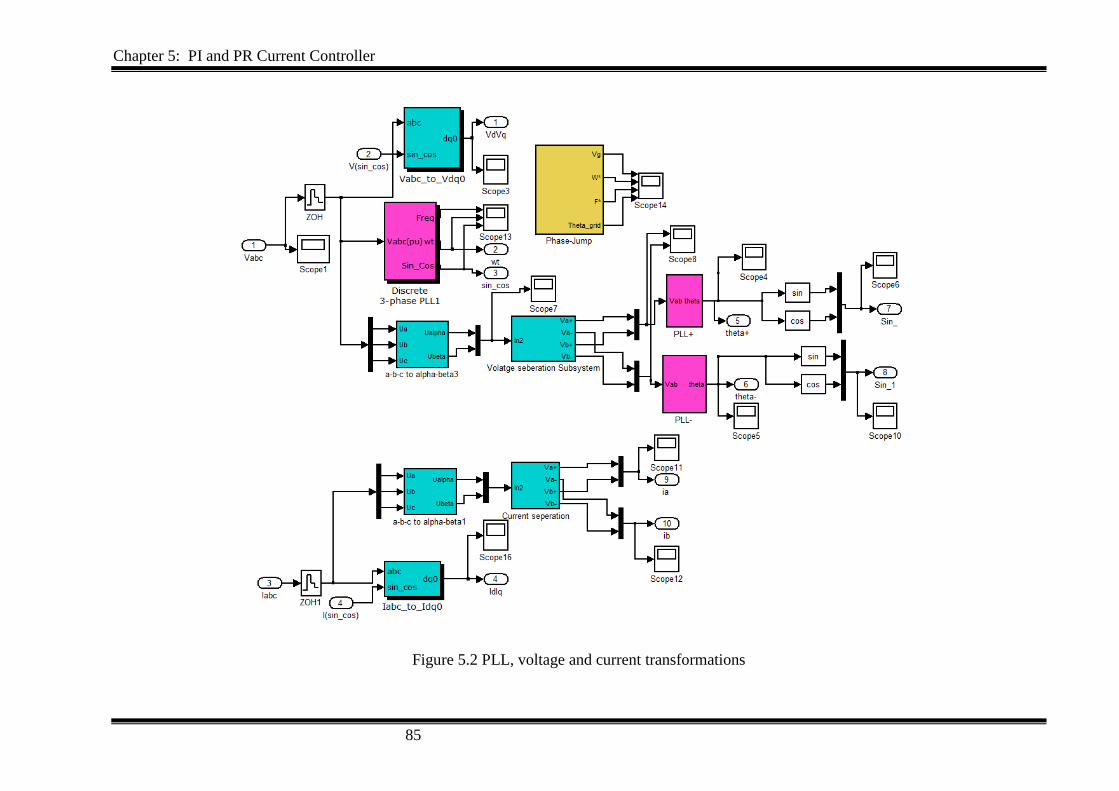
Chapter 5: PI and PR Current Controller
85
Figure 5.2 PLL, voltage and current transformations
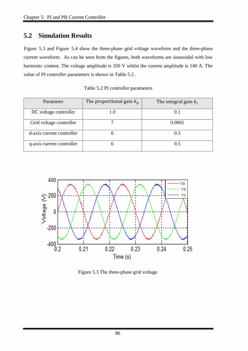
Chapter 5: PI and PR Current Controller
86
5.2 Simulation Results
Figure 5.3 and Figure 5.4 show the three-phase grid voltage waveform and the three-phase
current waveform. As can be seen from the figures, both waveforms are sinusoidal with low
harmonic content. The voltage amplitude is 350 V whilst the current amplitude is 140 A. The
value of PI controller parameters is shown in Table 5.2 .
Table 5.2 PI controller parameters
Parameter The proportional gain 𝑘𝑝 The integral gain 𝑘𝑖
DC voltage controller 1.0 0.1
Grid voltage controller 7 0.0001
d-axis current controller 6 0.5
q-axis current controller 6 0.5
Figure 5.3 The three-phase grid voltage
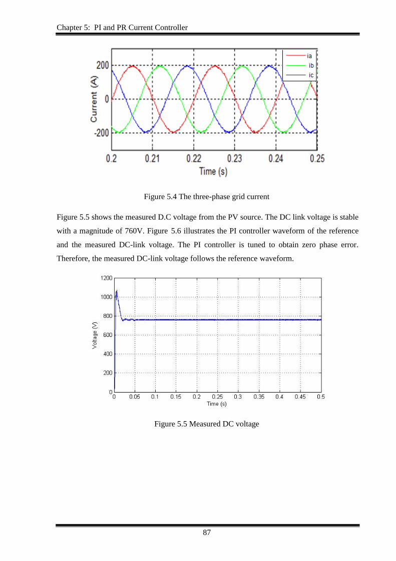
Chapter 5: PI and PR Current Controller
87
Figure 5.4 The three-phase grid current
Figure 5.5 shows the measured D.C voltage from the PV source. The DC link voltage is stable
with a magnitude of 760V. Figure 5.6 illustrates the PI controller waveform of the reference
and the measured DC-link voltage. The PI controller is tuned to obtain zero phase error.
Therefore, the measured DC-link voltage follows the reference waveform.
Figure 5.5 Measured DC voltage
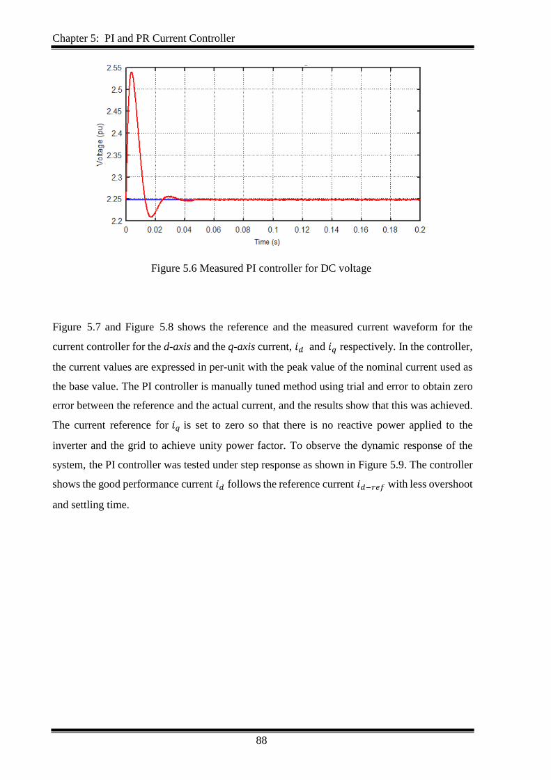
Chapter 5: PI and PR Current Controller
88
Figure 5.6 Measured PI controller for DC voltage
Figure 5.7 and Figure 5.8 shows the reference and the measured current waveform for the
current controller for the d-axis and the q-axis current, 𝑖𝑑 and 𝑖𝑞 respectively. In the controller,
the current values are expressed in per-unit with the peak value of the nominal current used as
the base value. The PI controller is manually tuned method using trial and error to obtain zero
error between the reference and the actual current, and the results show that this was achieved.
The current reference for 𝑖𝑞 is set to zero so that there is no reactive power applied to the
inverter and the grid to achieve unity power factor. To observe the dynamic response of the
system, the PI controller was tested under step response as shown in Figure 5.9. The controller
shows the good performance current 𝑖𝑑 follows the reference current 𝑖𝑑−𝑟𝑒𝑓 with less overshoot
and settling time.
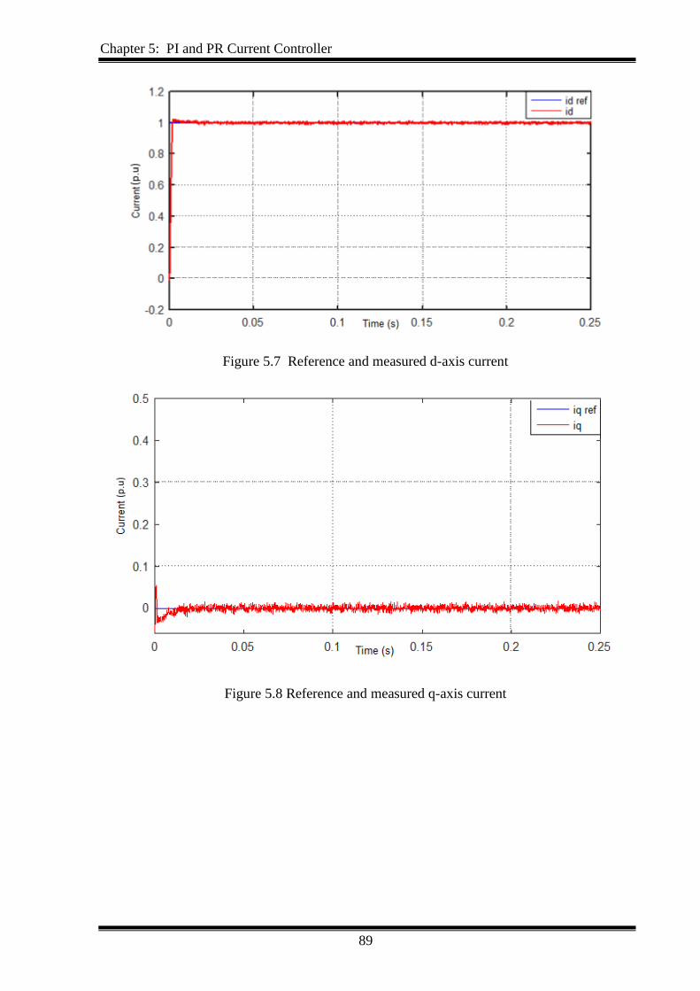
Chapter 5: PI and PR Current Controller
89
Figure 5.7 Reference and measured d-axis current
Figure 5.8 Reference and measured q-axis current
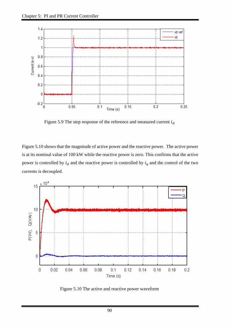
Chapter 5: PI and PR Current Controller
90
Figure 5.9 The step response of the reference and measured current 𝑖𝑑
Figure 5.10 shows that the magnitude of active power and the reactive power. The active power
is at its nominal value of 100 kW while the reactive power is zero. This confirms that the active
power is controlled by 𝑖𝑑 and the reactive power is controlled by 𝑖𝑞 and the control of the two
currents is decoupled.
Figure 5.10 The active and reactive power waveform

Chapter 5: PI and PR Current Controller
91
5.2.1 PI controller under abnormal grid conditions
This section investigates the performance of the control technique under abnormal grid
conditions. The abnormal grid conditions are faults which lead to voltage sags or swell at the
inverter terminals. Most common of abnormal conditions and power quality refers to voltage
sags. Two possible scenarios have been considered, the first one considers is a balanced three-
phase fault leading to a voltage sag of 75% of the rated voltage for the time interval of 0.1-0.15
seconds and voltage swell of 30% from 0.17-0.19 seconds. Whilst the second case analyses an
unbalanced voltage sag of 90% of the nominal voltage applied to two phases of the gird-
connected inverter.
5.2.1.1 PI controller under balanced voltage sag
Figure 5.11 shows the three-phase voltage waveform during the balanced voltage sag and swell
disturbance. It can be seen that the voltage magnitude in all the phases is reduced equally, but
the waveforms are not distorted. Figure 5.12 shows the three-phase current waveform during
the balanced voltage sag and swell. There is an increase in the magnitude of the current during
the fault at a time interval of 0.1-0.15 seconds and decreased from 0.17-0.19 seconds. This is
because the same amount of active power has to flow from the PV array to the grid before and
during the voltage sag. Therefore, when the voltage decreases, the current has to increase to
maintain the flow of active power.
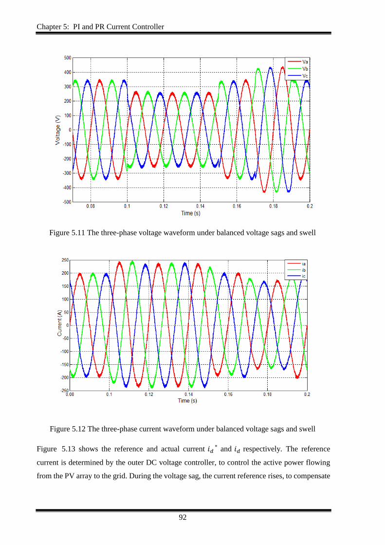
Chapter 5: PI and PR Current Controller
92
Figure 5.11 The three-phase voltage waveform under balanced voltage sags and swell
Figure 5.12 The three-phase current waveform under balanced voltage sags and swell
Figure 5.13 shows the reference and actual current 𝑖𝑑* and 𝑖𝑑 respectively. The reference
current is determined by the outer DC voltage controller, to control the active power flowing
from the PV array to the grid. During the voltage sag, the current reference rises, to compensate
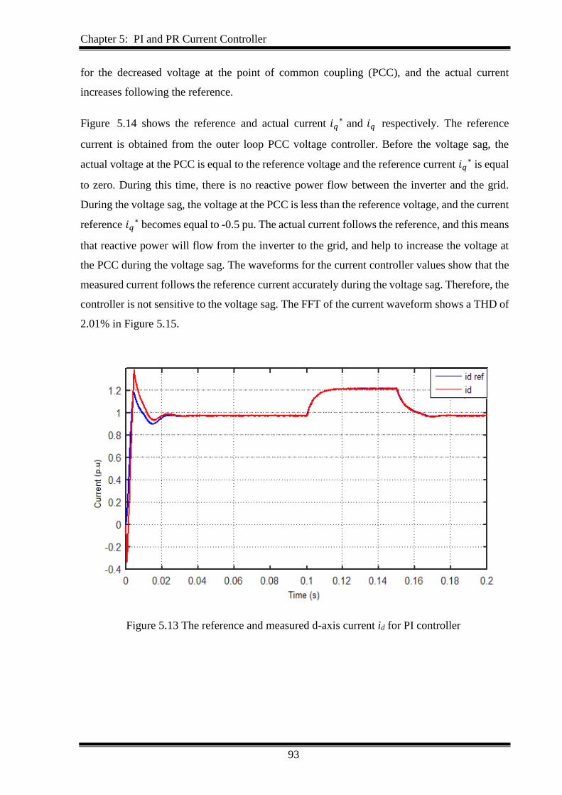
Chapter 5: PI and PR Current Controller
93
for the decreased voltage at the point of common coupling (PCC), and the actual current
increases following the reference.
Figure 5.14 shows the reference and actual current 𝑖𝑞∗ and 𝑖𝑞 respectively. The reference
current is obtained from the outer loop PCC voltage controller. Before the voltage sag, the
actual voltage at the PCC is equal to the reference voltage and the reference current 𝑖𝑞∗ is equal
to zero. During this time, there is no reactive power flow between the inverter and the grid.
During the voltage sag, the voltage at the PCC is less than the reference voltage, and the current
reference 𝑖𝑞∗ becomes equal to -0.5 pu. The actual current follows the reference, and this means
that reactive power will flow from the inverter to the grid, and help to increase the voltage at
the PCC during the voltage sag. The waveforms for the current controller values show that the
measured current follows the reference current accurately during the voltage sag. Therefore, the
controller is not sensitive to the voltage sag. The FFT of the current waveform shows a THD of
2.01% in Figure 5.15.
Figure 5.13 The reference and measured d-axis current id for PI controller
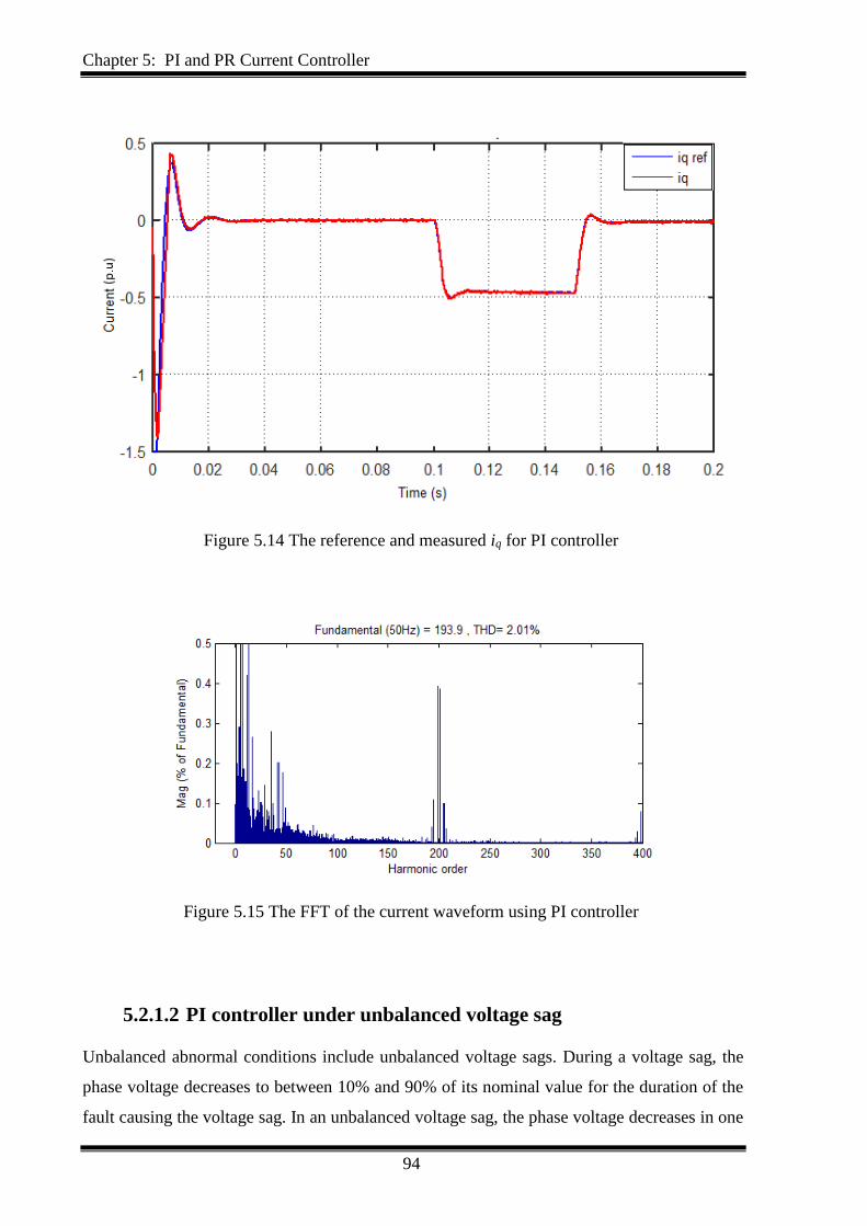
Chapter 5: PI and PR Current Controller
94
Figure 5.14 The reference and measured iq for PI controller
Figure 5.15 The FFT of the current waveform using PI controller
5.2.1.2 PI controller under unbalanced voltage sag
Unbalanced abnormal conditions include unbalanced voltage sags. During a voltage sag, the
phase voltage decreases to between 10% and 90% of its nominal value for the duration of the
fault causing the voltage sag. In an unbalanced voltage sag, the phase voltage decreases in one
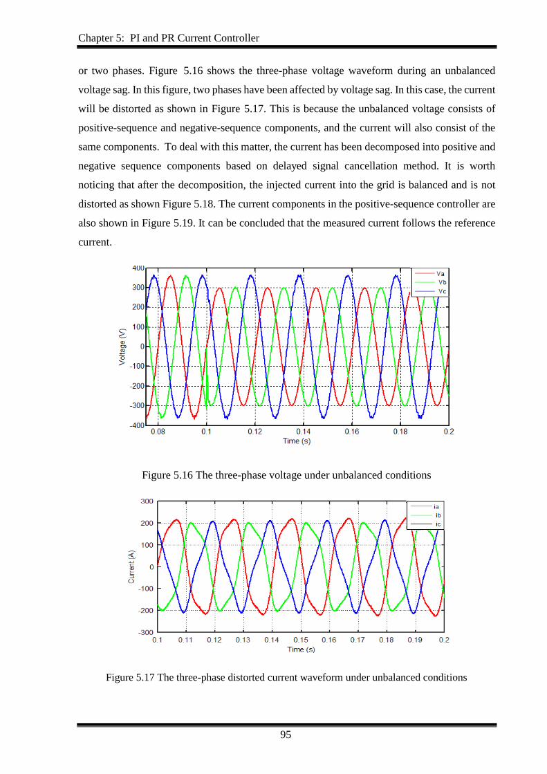
Chapter 5: PI and PR Current Controller
95
or two phases. Figure 5.16 shows the three-phase voltage waveform during an unbalanced
voltage sag. In this figure, two phases have been affected by voltage sag. In this case, the current
will be distorted as shown in Figure 5.17. This is because the unbalanced voltage consists of
positive-sequence and negative-sequence components, and the current will also consist of the
same components. To deal with this matter, the current has been decomposed into positive and
negative sequence components based on delayed signal cancellation method. It is worth
noticing that after the decomposition, the injected current into the grid is balanced and is not
distorted as shown Figure 5.18. The current components in the positive-sequence controller are
also shown in Figure 5.19. It can be concluded that the measured current follows the reference
current.
Figure 5.16 The three-phase voltage under unbalanced conditions
Figure 5.17 The three-phase distorted current waveform under unbalanced conditions
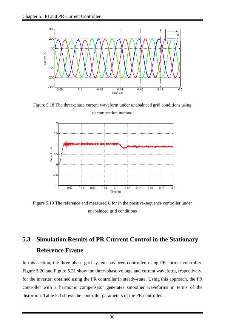
Chapter 5: PI and PR Current Controller
96
Figure 5.18 The three-phase current waveform under unabalnced grid conditions using
decompestion method
Figure 5.19 The reference and measured id for in the positive-sequence controller under
unabalnced grid conditions
5.3 Simulation Results of PR Current Control in the Stationary
Reference Frame
In this section, the three-phase grid system has been controlled using PR current controller.
Figure 5.20 and Figure 5.21 show the three-phase voltage and current waveform, respectively,
for the inverter, obtained using the PR controller in steady-state. Using this approach, the PR
controller with a harmonic compensator generates smoother waveforms in terms of the
distortion. Table 5.3 shows the controller parameters of the PR controller.
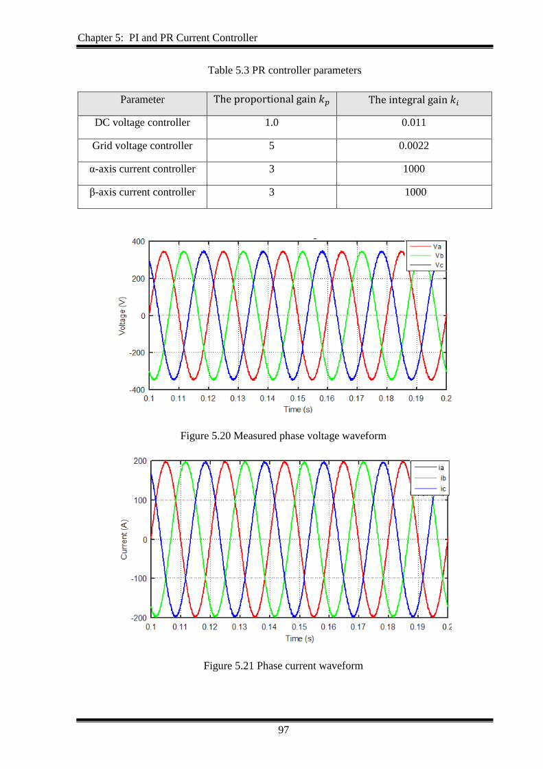
Chapter 5: PI and PR Current Controller
97
Table 5.3 PR controller parameters
Parameter The proportional gain 𝑘𝑝 The integral gain 𝑘𝑖
DC voltage controller 1.0 0.011
Grid voltage controller 5 0.0022
α-axis current controller 3 1000
β-axis current controller 3 1000
Figure 5.20 Measured phase voltage waveform
Figure 5.21 Phase current waveform
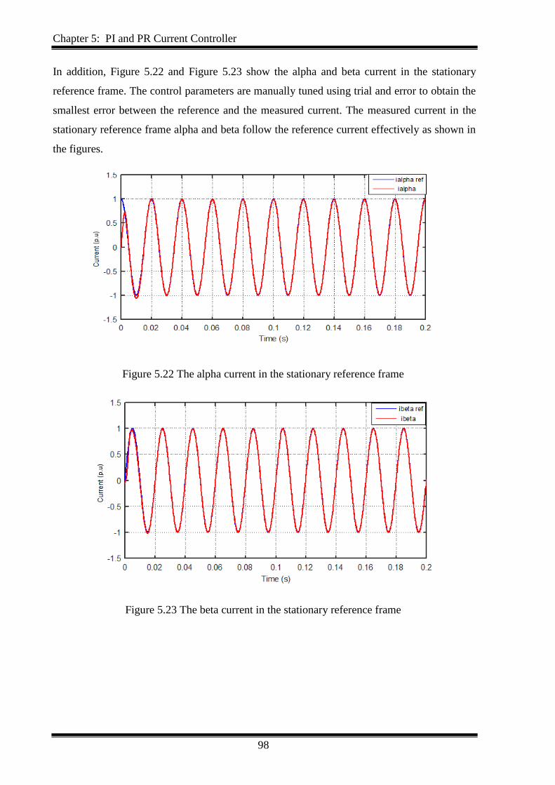
Chapter 5: PI and PR Current Controller
98
In addition, Figure 5.22 and Figure 5.23 show the alpha and beta current in the stationary
reference frame. The control parameters are manually tuned using trial and error to obtain the
smallest error between the reference and the measured current. The measured current in the
stationary reference frame alpha and beta follow the reference current effectively as shown in
the figures.
Figure 5.22 The alpha current in the stationary reference frame
Figure 5.23 The beta current in the stationary reference frame

Chapter 5: PI and PR Current Controller
99
5.3.1 PR controller under abnormal grid conditions
The performance of the PR controller has been experienced in abnormal grid condition
considering two cases. In the first case, three-phase voltage sag is applied at a time of 0.15 sec
as shown in Figure 5.24. Figure 5.25 shows the current waveform under voltage sag. It can be
seen from the Figure 5.24 and Figure 5.25 that the result is satisfactory in both transient and
steady state.
Figure 5.24 The three-phase grid voltage waveform under voltage sags
Figure 5.25 The three-phase current using PR controller
Despite the PR controller offers good performance during abnormal grid conditions. However,
a sudden change in the grid such as the drop or the increased in the voltage could show a rise
in regard to the error between the reference signal and the controlled signal. This, in turn, would
seemingly cause a noticeable divergence from its nominal value in the transient response. In
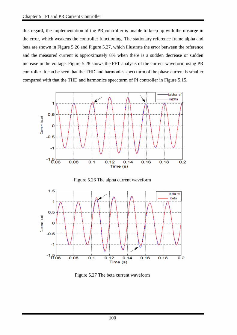
Chapter 5: PI and PR Current Controller
100
this regard, the implementation of the PR controller is unable to keep up with the upsurge in
the error, which weakens the controller functioning. The stationary reference frame alpha and
beta are shown in Figure 5.26 and Figure 5.27, which illustrate the error between the reference
and the measured current is approximately 8% when there is a sudden decrease or sudden
increase in the voltage. Figure 5.28 shows the FFT analysis of the current waveform using PR
controller. It can be seen that the THD and harmonics speccturm of the phase current is smaller
compared with that the THD and harmonics speccturm of PI controller in Figure 5.15.
Figure 5.26 The alpha current waveform
Figure 5.27 The beta current waveform
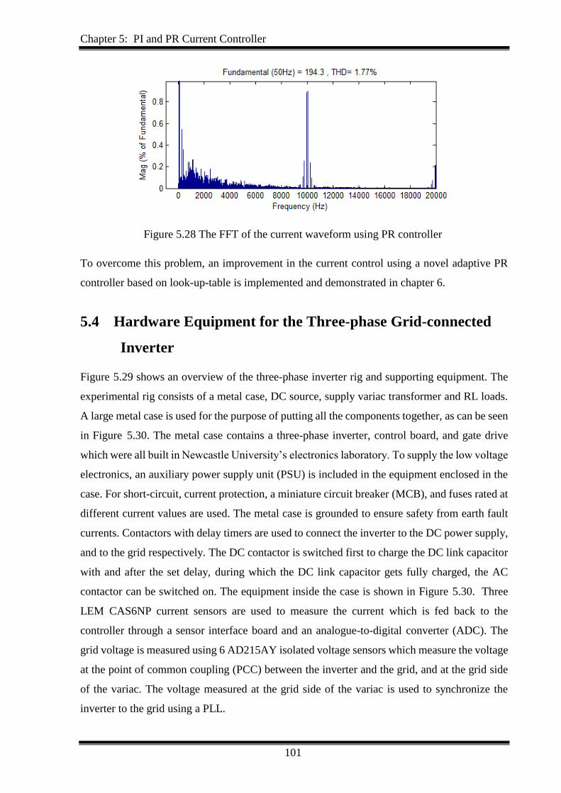
Chapter 5: PI and PR Current Controller
101
Figure 5.28 The FFT of the current waveform using PR controller
To overcome this problem, an improvement in the current control using a novel adaptive PR
controller based on look-up-table is implemented and demonstrated in chapter 6.
5.4 Hardware Equipment for the Three-phase Grid-connected
Inverter
Figure 5.29 shows an overview of the three-phase inverter rig and supporting equipment. The
experimental rig consists of a metal case, DC source, supply variac transformer and RL loads.
A large metal case is used for the purpose of putting all the components together, as can be seen
in Figure 5.30. The metal case contains a three-phase inverter, control board, and gate drive
which were all built in Newcastle University’s electronics laboratory. To supply the low voltage
electronics, an auxiliary power supply unit (PSU) is included in the equipment enclosed in the
case. For short-circuit, current protection, a miniature circuit breaker (MCB), and fuses rated at
different current values are used. The metal case is grounded to ensure safety from earth fault
currents. Contactors with delay timers are used to connect the inverter to the DC power supply,
and to the grid respectively. The DC contactor is switched first to charge the DC link capacitor
with and after the set delay, during which the DC link capacitor gets fully charged, the AC
contactor can be switched on. The equipment inside the case is shown in Figure 5.30. Three
LEM CAS6NP current sensors are used to measure the current which is fed back to the
controller through a sensor interface board and an analogue-to-digital converter (ADC). The
grid voltage is measured using 6 AD215AY isolated voltage sensors which measure the voltage
at the point of common coupling (PCC) between the inverter and the grid, and at the grid side
of the variac. The voltage measured at the grid side of the variac is used to synchronize the
inverter to the grid using a PLL.
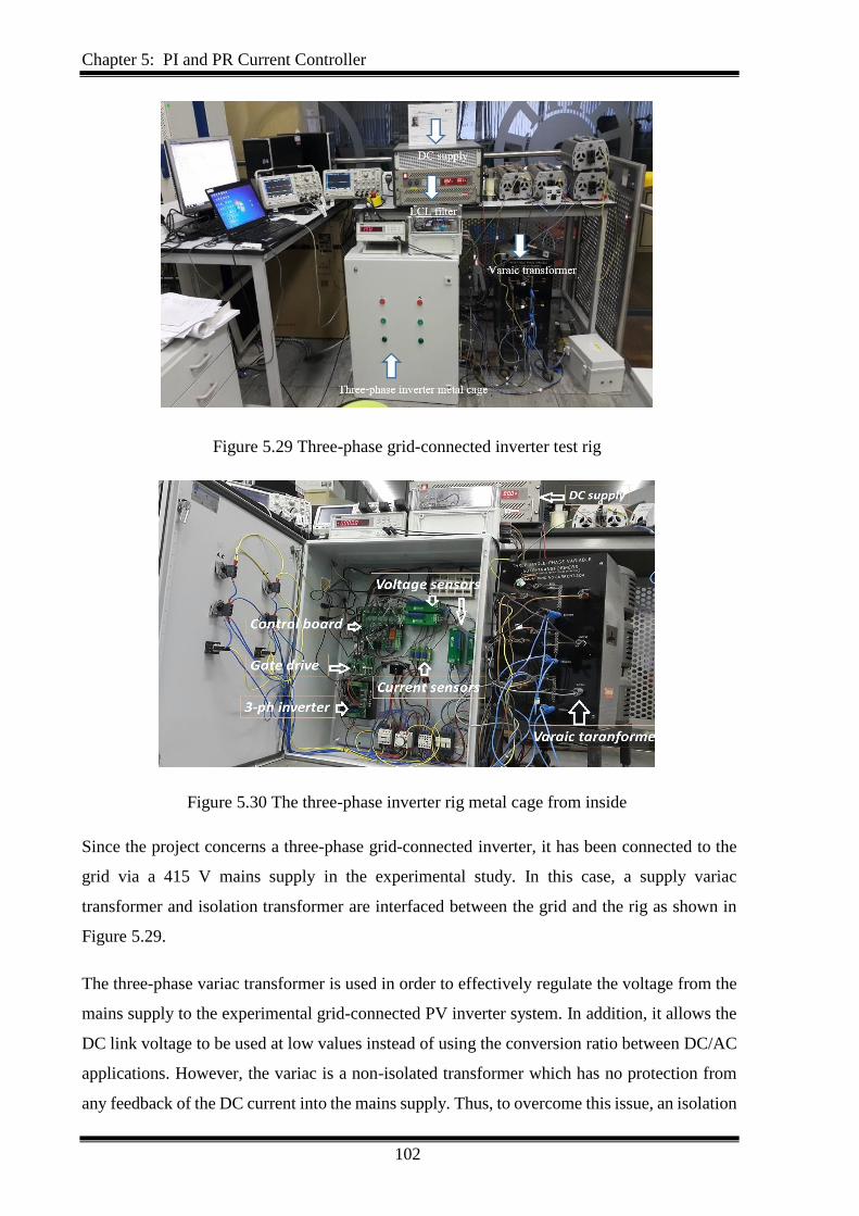
Chapter 5: PI and PR Current Controller
102
Figure 5.29 Three-phase grid-connected inverter test rig
Figure 5.30 The three-phase inverter rig metal cage from inside
Since the project concerns a three-phase grid-connected inverter, it has been connected to the
grid via a 415 V mains supply in the experimental study. In this case, a supply variac
transformer and isolation transformer are interfaced between the grid and the rig as shown in
Figure 5.29.
The three-phase variac transformer is used in order to effectively regulate the voltage from the
mains supply to the experimental grid-connected PV inverter system. In addition, it allows the
DC link voltage to be used at low values instead of using the conversion ratio between DC/AC
applications. However, the variac is a non-isolated transformer which has no protection from
any feedback of the DC current into the mains supply. Thus, to overcome this issue, an isolation
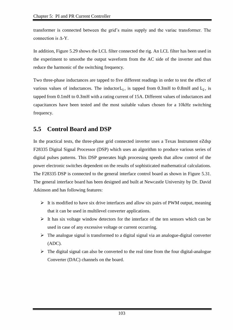
Chapter 5: PI and PR Current Controller
103
transformer is connected between the grid’s mains supply and the variac transformer. The
connection is Δ-Y.
In addition, Figure 5.29 shows the LCL filter connected the rig. An LCL filter has been used in
the experiment to smoothe the output waveform from the AC side of the inverter and thus
reduce the harmonic of the switching frequency.
Two three-phase inductances are tapped to five different readings in order to test the effect of
various values of inductances. The inductorL1 , is tapped from 0.3mH to 0.8mH and L2 , is
tapped from 0.1mH to 0.3mH with a rating current of 15A. Different values of inductances and
capacitances have been tested and the most suitable values chosen for a 10kHz switching
frequency.
5.5 Control Board and DSP
In the practical tests, the three-phase grid connected inverter uses a Texas Instrument eZdsp
F28335 Digital Signal Processor (DSP) which uses an algorithm to produce various series of
digital pulses patterns. This DSP generates high processing speeds that allow control of the
power electronic switches dependent on the results of sophisticated mathematical calculations.
The F28335 DSP is connected to the general interface control board as shown in Figure 5.31.
The general interface board has been designed and built at Newcastle University by Dr. David
Atkinson and has following features:
It is modified to have six drive interfaces and allow six pairs of PWM output, meaning
that it can be used in multilevel converter applications.
It has six voltage window detectors for the interface of the ten sensors which can be
used in case of any excessive voltage or current occurring.
The analogue signal is transformed to a digital signal via an analogue-digital converter
(ADC).
The digital signal can also be converted to the real time from the four digital-analogue
Converter (DAC) channels on the board.
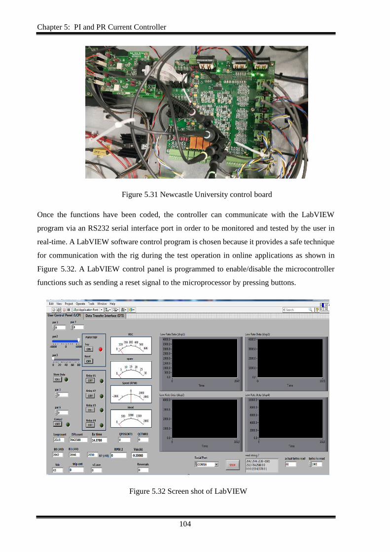
Chapter 5: PI and PR Current Controller
104
Figure 5.31 Newcastle University control board
Once the functions have been coded, the controller can communicate with the LabVIEW
program via an RS232 serial interface port in order to be monitored and tested by the user in
real-time. A LabVIEW software control program is chosen because it provides a safe technique
for communication with the rig during the test operation in online applications as shown in
Figure 5.32. A LabVIEW control panel is programmed to enable/disable the microcontroller
functions such as sending a reset signal to the microprocessor by pressing buttons.
Figure 5.32 Screen shot of LabVIEW

Chapter 5: PI and PR Current Controller
105
5.6 Power Wiring Diagram
The experimental system is designed and installed to provide interaction between PV sources
and the utility grid in the UG lab bay A. Figure 5.33 shows a general overview of the power
wiring diagram for the rig. A three-phase inverter is supplied by a DC source and connected to
the LCL filter. The rig has two DC switching contactor (D1 and D2) from the DC side and one
contactor (A) from the AC side along with the main MCB for safety and emergency purposes.
When the DC link is switched on, a high inrush current will flow into the DC link circuit. A
timer delay is connected to the contactor (D2) to hold it for a few seconds in order to allow the
DC capacitors to charge up. A resistor is connected in parallel with the contactor and a diode is
connected on the DC side to prevent the reversal of the current into the DC power supply. In
addition, the rig has one voltage sensor on the DC link voltage, three voltage sensors in the AC
side and three current sensors also on the AC side. In order to protect the DC link capacitors
from excessive current, a fast fuse is placed before the output of the three-phase inverter which
has the ability to blow up in case of over-current.
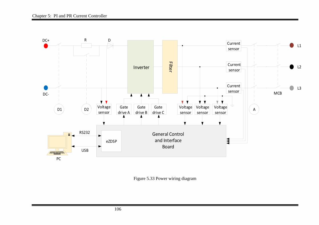
Chapter 5: PI and PR Current Controller
106
eZDSP
PC
R D
Inverter
Filte
r
RS232
USB
D1 D2 A
DC+
DC-
Voltage sensor
Voltage sensor
Voltage sensor
Currentsensor
Currentsensor
Currentsensor
Gate drive A
Gate drive B
Gate drive C
General Control and Interface
Board
L1
L2
L3MCB
Voltage sensor
Figure 5.33 Power wiring diagram

Chapter 5: PI and PR Current Controller
107
5.7 Grid Connection Sequence
In order to connect the three-phase inverter to the grid, the following procedures are employed:
1. All AC and DC switches are switched off.
2. The three-phase variac is set to zero voltage to make sure that no voltage is applied to
the system.
3. The program code is run and it is checked that the phase-locked loop is working.
4. The DC supply is switched on to charge the capacitors and after a few seconds, the AC
side is switched on.
5. The three-phase variac is gradually increased and DC link voltage is established to feed
the inverter input until it reaches the maximum allowable values. However, the current
demand is still kept at zero.
6. The LabVIEW control program is switched on and the current demand is gradually
increased in order to deliver the current to the grid network.
5.8 Experimental Results of PI and PR Controller
To validate the control technique for the system in the laboratory, the system is scaled down
and has been tested, the specifications of the system parameters have been accurately chosen
based on mathematical equations [146-148]. The experimental parameters are calculated based
on equations (5.1) to (5.10). The nominal operating parameters are shown in Table 5.4.
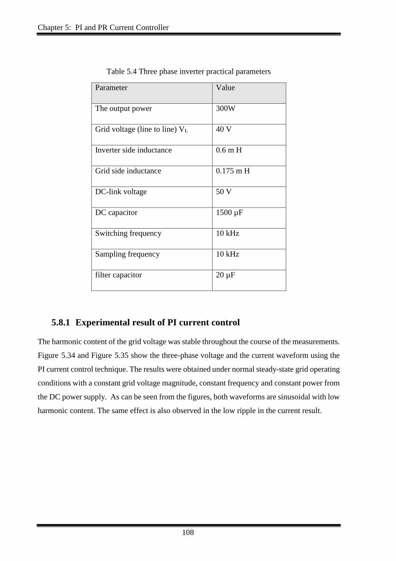
Chapter 5: PI and PR Current Controller
108
Table 5.4 Three phase inverter practical parameters
Parameter Value
The output power 300W
Grid voltage (line to line) VL 40 V
Inverter side inductance 0.6 m H
Grid side inductance 0.175 m H
DC-link voltage 50 V
DC capacitor 1500 µF
Switching frequency 10 kHz
Sampling frequency 10 kHz
filter capacitor 20 µF
5.8.1 Experimental result of PI current control
The harmonic content of the grid voltage was stable throughout the course of the measurements.
Figure 5.34 and Figure 5.35 show the three-phase voltage and the current waveform using the
PI current control technique. The results were obtained under normal steady-state grid operating
conditions with a constant grid voltage magnitude, constant frequency and constant power from
the DC power supply. As can be seen from the figures, both waveforms are sinusoidal with low
harmonic content. The same effect is also observed in the low ripple in the current result.
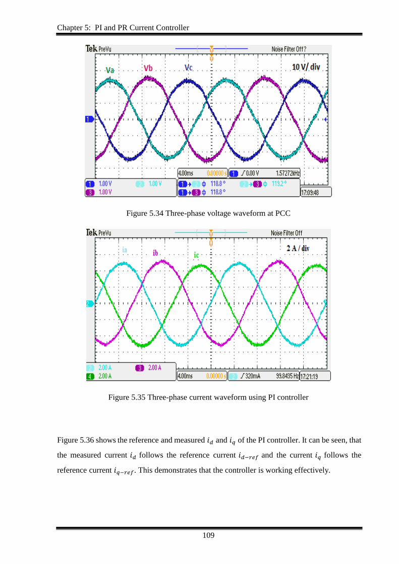
Chapter 5: PI and PR Current Controller
109
Figure 5.34 Three-phase voltage waveform at PCC
Figure 5.35 Three-phase current waveform using PI controller
Figure 5.36 shows the reference and measured 𝑖𝑑 and 𝑖𝑞 of the PI controller. It can be seen, that
the measured current 𝑖𝑑 follows the reference current 𝑖𝑑−𝑟𝑒𝑓 and the current 𝑖𝑞 follows the
reference current 𝑖𝑞−𝑟𝑒𝑓. This demonstrates that the controller is working effectively.
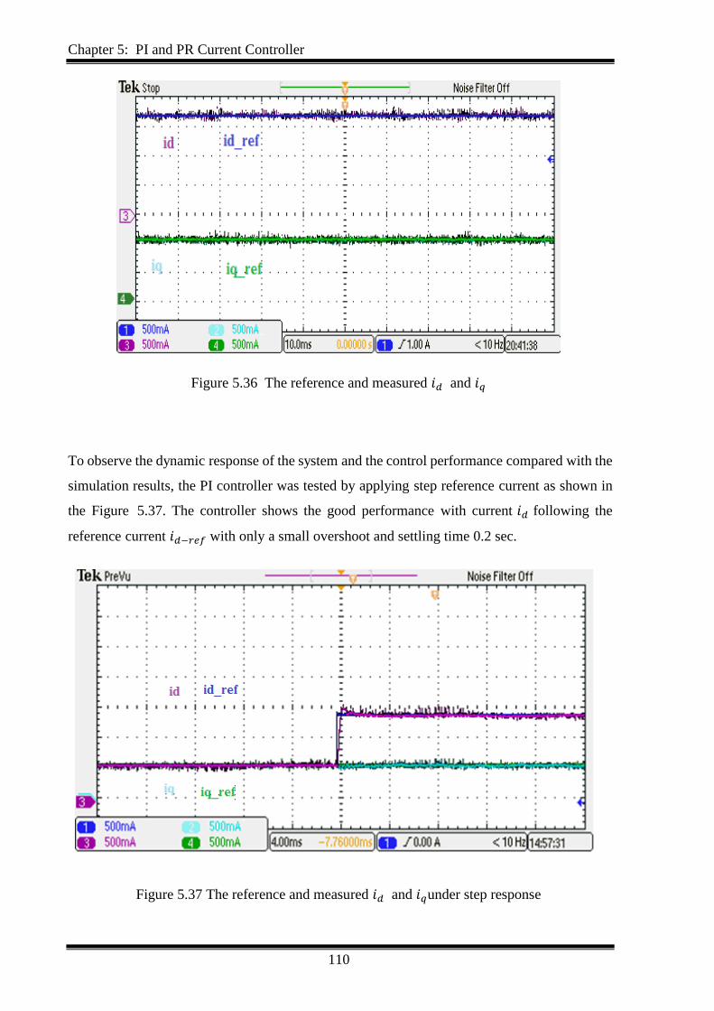
Chapter 5: PI and PR Current Controller
110
Figure 5.36 The reference and measured 𝑖𝑑 and 𝑖𝑞
To observe the dynamic response of the system and the control performance compared with the
simulation results, the PI controller was tested by applying step reference current as shown in
the Figure 5.37. The controller shows the good performance with current 𝑖𝑑 following the
reference current 𝑖𝑑−𝑟𝑒𝑓 with only a small overshoot and settling time 0.2 sec.
Figure 5.37 The reference and measured 𝑖𝑑 and 𝑖𝑞under step response
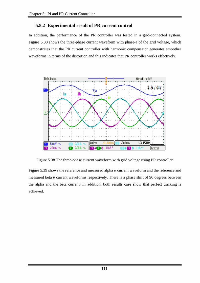
Chapter 5: PI and PR Current Controller
111
5.8.2 Experimental result of PR current control
In addition, the performance of the PR controller was tested in a grid-connected system.
Figure 5.38 shows the three-phase current waveform with phase-a of the grid voltage, which
demonstrates that the PR current controller with harmonic compensator generates smoother
waveforms in terms of the distortion and this indicates that PR controller works effectively.
Figure 5.38 The three-phase current waveform with grid voltage using PR controller
Figure 5.39 shows the reference and measured alpha α current waveform and the reference and
measured beta β current waveforms respectively. There is a phase shift of 90 degrees between
the alpha and the beta current. In addition, both results case show that perfect tracking is
achieved.
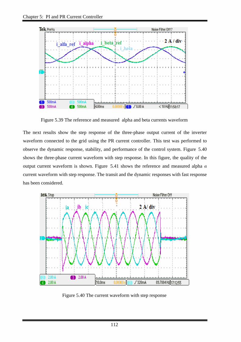
Chapter 5: PI and PR Current Controller
112
Figure 5.39 The reference and measured alpha and beta currents waveform
The next results show the step response of the three-phase output current of the inverter
waveform connected to the grid using the PR current controller. This test was performed to
observe the dynamic response, stability, and performance of the control system. Figure 5.40
shows the three-phase current waveform with step response. In this figure, the quality of the
output current waveform is shown. Figure 5.41 shows the reference and measured alpha α
current waveform with step response. The transit and the dynamic responses with fast response
has been considered.
Figure 5.40 The current waveform with step response
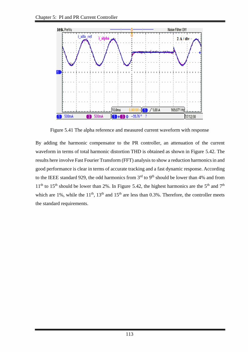
Chapter 5: PI and PR Current Controller
113
Figure 5.41 The alpha reference and measured current waveform with response
By adding the harmonic compensator to the PR controller, an attenuation of the current
waveform in terms of total harmonic distortion THD is obtained as shown in Figure 5.42. The
results here involve Fast Fourier Transform (FFT) analysis to show a reduction harmonics in and
good performance is clear in terms of accurate tracking and a fast dynamic response. According
to the IEEE standard 929, the odd harmonics from 3rd to 9th should be lower than 4% and from
11th to 15th should be lower than 2%. In Figure 5.42, the highest harmonics are the 5th and 7th
which are 1%, while the 11th, 13th and 15th are less than 0.3%. Therefore, the controller meets
the standard requirements.
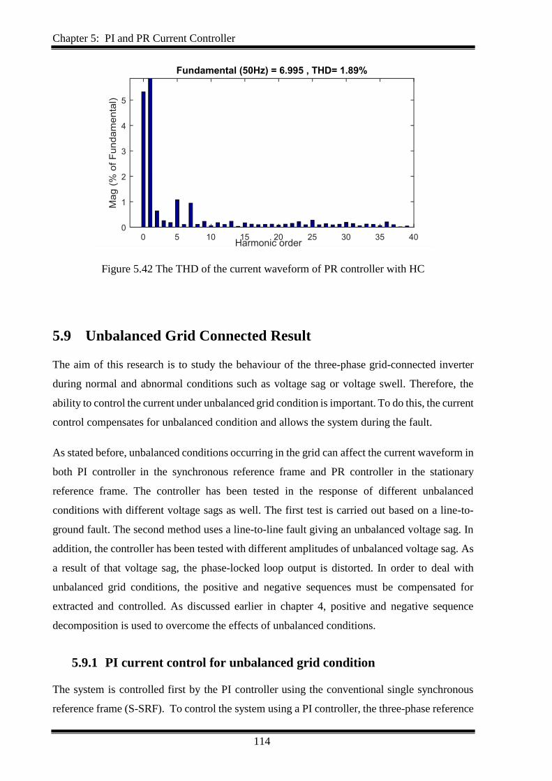
Chapter 5: PI and PR Current Controller
114
Figure 5.42 The THD of the current waveform of PR controller with HC
5.9 Unbalanced Grid Connected Result
The aim of this research is to study the behaviour of the three-phase grid-connected inverter
during normal and abnormal conditions such as voltage sag or voltage swell. Therefore, the
ability to control the current under unbalanced grid condition is important. To do this, the current
control compensates for unbalanced condition and allows the system during the fault.
As stated before, unbalanced conditions occurring in the grid can affect the current waveform in
both PI controller in the synchronous reference frame and PR controller in the stationary
reference frame. The controller has been tested in the response of different unbalanced
conditions with different voltage sags as well. The first test is carried out based on a line-to-
ground fault. The second method uses a line-to-line fault giving an unbalanced voltage sag. In
addition, the controller has been tested with different amplitudes of unbalanced voltage sag. As
a result of that voltage sag, the phase-locked loop output is distorted. In order to deal with
unbalanced grid conditions, the positive and negative sequences must be compensated for
extracted and controlled. As discussed earlier in chapter 4, positive and negative sequence
decomposition is used to overcome the effects of unbalanced conditions.
5.9.1 PI current control for unbalanced grid condition
The system is controlled first by the PI controller using the conventional single synchronous
reference frame (S-SRF). To control the system using a PI controller, the three-phase reference
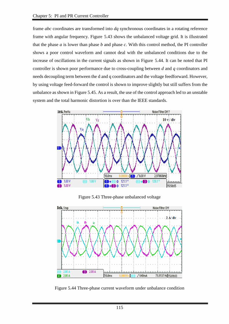
Chapter 5: PI and PR Current Controller
115
frame abc coordinates are transformed into dq synchronous coordinates in a rotating reference
frame with angular frequency. Figure 5.43 shows the unbalanced voltage grid. It is illustrated
that the phase a is lower than phase b and phase c. With this control method, the PI controller
shows a poor control waveform and cannot deal with the unbalanced conditions due to the
increase of oscillations in the current signals as shown in Figure 5.44. It can be noted that PI
controller is shown poor performance due to cross-coupling between d and q coordinators and
needs decoupling term between the d and q coordinators and the voltage feedforward. However,
by using voltage feed-forward the control is shown to improve slightly but still suffers from the
unbalance as shown in Figure 5.45. As a result, the use of the control approach led to an unstable
system and the total harmonic distortion is over than the IEEE standards.
Figure 5.43 Three-phase unbalanced voltage
Figure 5.44 Three-phase current waveform under unbalance condition
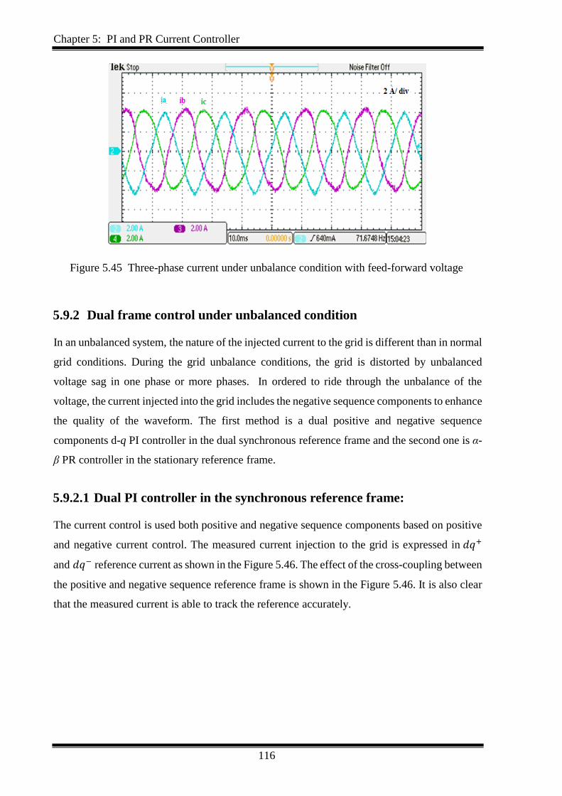
Chapter 5: PI and PR Current Controller
116
Figure 5.45 Three-phase current under unbalance condition with feed-forward voltage
5.9.2 Dual frame control under unbalanced condition
In an unbalanced system, the nature of the injected current to the grid is different than in normal
grid conditions. During the grid unbalance conditions, the grid is distorted by unbalanced
voltage sag in one phase or more phases. In ordered to ride through the unbalance of the
voltage, the current injected into the grid includes the negative sequence components to enhance
the quality of the waveform. The first method is a dual positive and negative sequence
components d-q PI controller in the dual synchronous reference frame and the second one is α-
β PR controller in the stationary reference frame.
5.9.2.1 Dual PI controller in the synchronous reference frame:
The current control is used both positive and negative sequence components based on positive
and negative current control. The measured current injection to the grid is expressed in 𝑑𝑞+
and 𝑑𝑞− reference current as shown in the Figure 5.46. The effect of the cross-coupling between
the positive and negative sequence reference frame is shown in the Figure 5.46. It is also clear
that the measured current is able to track the reference accurately.
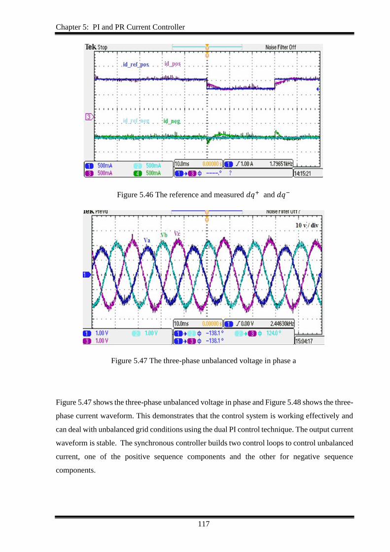
Chapter 5: PI and PR Current Controller
117
Figure 5.46 The reference and measured 𝑑𝑞+ and 𝑑𝑞−
Figure 5.47 The three-phase unbalanced voltage in phase a
Figure 5.47 shows the three-phase unbalanced voltage in phase and Figure 5.48 shows the three-
phase current waveform. This demonstrates that the control system is working effectively and
can deal with unbalanced grid conditions using the dual PI control technique. The output current
waveform is stable. The synchronous controller builds two control loops to control unbalanced
current, one of the positive sequence components and the other for negative sequence
components.
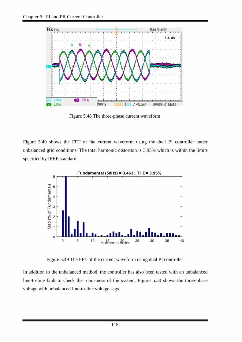
Chapter 5: PI and PR Current Controller
118
Figure 5.48 The three-phase current waveform
Figure 5.49 shows the FFT of the current waveform using the dual PI controller under
unbalanced grid conditions. The total harmonic distortion is 3.95% which is within the limits
specified by IEEE standard.
Figure 5.49 The FFT of the current waveform using dual PI controller
In addition to the unbalanced method, the controller has also been tested with an unbalanced
line-to-line fault to check the robustness of the system. Figure 5.50 shows the three-phase
voltage with unbalanced line-to-line voltage sags.
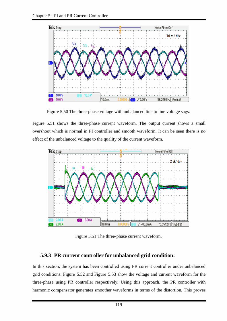
Chapter 5: PI and PR Current Controller
119
Figure 5.50 The three-phase voltage with unbalanced line to line voltage sags.
Figure 5.51 shows the three-phase current waveform. The output current shows a small
overshoot which is normal in PI controller and smooth waveform. It can be seen there is no
effect of the unbalanced voltage to the quality of the current waveform.
Figure 5.51 The three-phase current waveform.
5.9.3 PR current controller for unbalanced grid condition:
In this section, the system has been controlled using PR current controller under unbalanced
grid conditions. Figure 5.52 and Figure 5.53 show the voltage and current waveform for the
three-phase using PR controller respectively. Using this approach, the PR controller with
harmonic compensator generates smoother waveforms in terms of the distortion. This proves
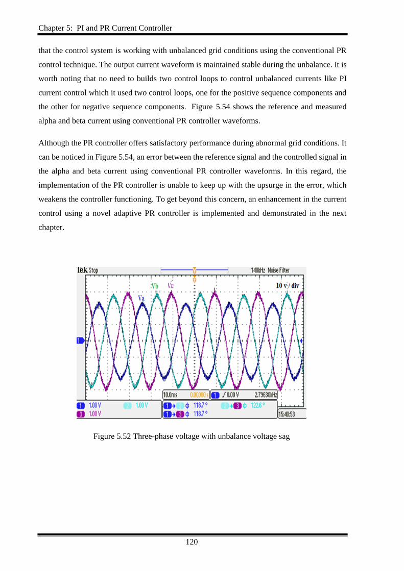
Chapter 5: PI and PR Current Controller
120
that the control system is working with unbalanced grid conditions using the conventional PR
control technique. The output current waveform is maintained stable during the unbalance. It is
worth noting that no need to builds two control loops to control unbalanced currents like PI
current control which it used two control loops, one for the positive sequence components and
the other for negative sequence components. Figure 5.54 shows the reference and measured
alpha and beta current using conventional PR controller waveforms.
Although the PR controller offers satisfactory performance during abnormal grid conditions. It
can be noticed in Figure 5.54, an error between the reference signal and the controlled signal in
the alpha and beta current using conventional PR controller waveforms. In this regard, the
implementation of the PR controller is unable to keep up with the upsurge in the error, which
weakens the controller functioning. To get beyond this concern, an enhancement in the current
control using a novel adaptive PR controller is implemented and demonstrated in the next
chapter.
Figure 5.52 Three-phase voltage with unbalance voltage sag
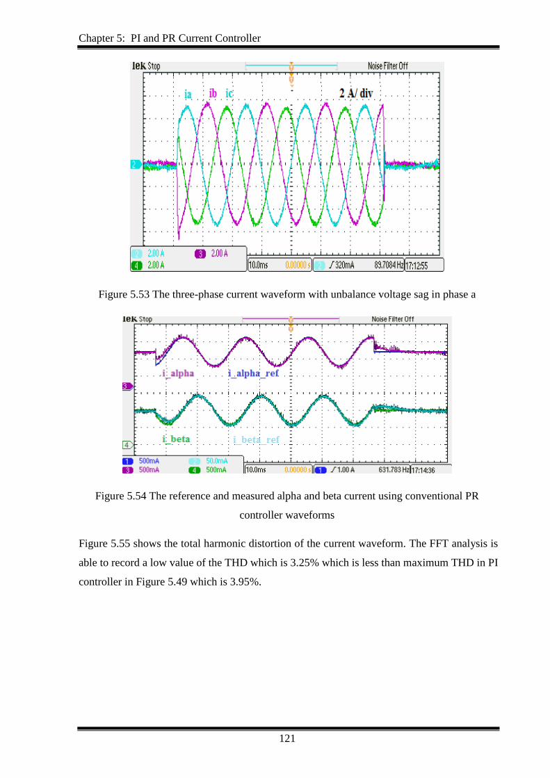
Chapter 5: PI and PR Current Controller
121
Figure 5.53 The three-phase current waveform with unbalance voltage sag in phase a
Figure 5.54 The reference and measured alpha and beta current using conventional PR
controller waveforms
Figure 5.55 shows the total harmonic distortion of the current waveform. The FFT analysis is
able to record a low value of the THD which is 3.25% which is less than maximum THD in PI
controller in Figure 5.49 which is 3.95%.
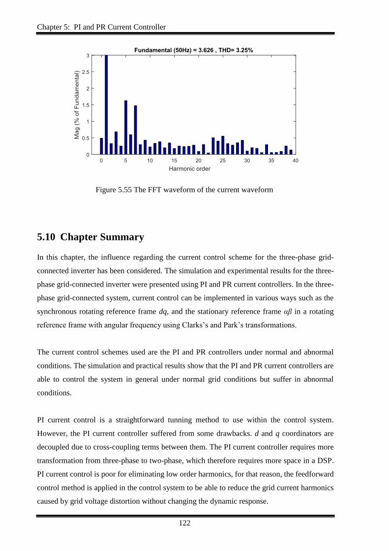
Chapter 5: PI and PR Current Controller
122
Figure 5.55 The FFT waveform of the current waveform
5.10 Chapter Summary
In this chapter, the influence regarding the current control scheme for the three-phase grid-
connected inverter has been considered. The simulation and experimental results for the three-
phase grid-connected inverter were presented using PI and PR current controllers. In the three-
phase grid-connected system, current control can be implemented in various ways such as the
synchronous rotating reference frame dq, and the stationary reference frame αβ in a rotating
reference frame with angular frequency using Clarks’s and Park’s transformations.
The current control schemes used are the PI and PR controllers under normal and abnormal
conditions. The simulation and practical results show that the PI and PR current controllers are
able to control the system in general under normal grid conditions but suffer in abnormal
conditions.
PI current control is a straightforward tunning method to use within the control system.
However, the PI current controller suffered from some drawbacks. d and q coordinators are
decoupled due to cross-coupling terms between them. The PI current controller requires more
transformation from three-phase to two-phase, which therefore requires more space in a DSP.
PI current control is poor for eliminating low order harmonics, for that reason, the feedforward
control method is applied in the control system to be able to reduce the grid current harmonics
caused by grid voltage distortion without changing the dynamic response.

Chapter 5: PI and PR Current Controller
123
Under abnormal grid conditions, the PI controller needs to control the positive and negative
voltage sequence separately, which makes the controller more complicated than before.
PR current control as another control method working in in the stationary reference frame. PR
current control is a straightforward method and has the capability to eliminate the steady state
error in normal grid conditions. In addition, PR controller can implement harmonic
compensator without changing the dynamic response. 𝛼 and 𝛽 coordinators are not decoupled
to each other. In abnormal grid conditions, PR controller can only control the positive voltage
sequence since both the positive and negative voltage components have the same fundamental
frequency. However, under abnormal grid conditions, the controlled signal instigating
significant deviation from its nominal value and causes an error which weakens controller
performance. As a result, a novel adaptive PR controller was implemented and tested in both
balanced and unbalanced grid conditions in the simulation and verified experimentally in the
following chapter.
Chapter 6: PI and PR Current Controller
124
Adaptive PR Controller
6.1 Introduction
In this chapter, the proposed adaptive PR controller is presented. The aim of this chapter is to
validate and prove the advantages of the proposed control approach in terms of stability and
minimizing the error between the measured and the reference controllers in the current
waveform during normal and abnormal grid conditions. The proposed technique is
implemented with the eZdsp F28335 and verified experimentally in normal and abnormal grid
conditions. The proposed control method is able to achieve better waveform with less overshoot
and less total harmonic distortion compared to PI controller and conventional PR controller.
6.2 Adaptive PR Controller
During abnormal grid conditions, the error between the references should be minimized to
within a very small limit. This requires appropriate adaptive control. In general, as 𝑘𝑝and
𝑘𝑖 increase, the gain and the bandwidth of the system is also increased. However, as the gain
increases, instability in the system can occur.
In the transient response, a large value of the 𝑘𝑝leads to an increase in the gains of all frequency
components, while 𝑘𝑖 decreases the settling time and helps reduce steady-state error and
therefore the higher the loop bandwidth, the better the transient performance [151]. When the
level of error suddenly increases beyond the maximum allowed variation of desired values in
the transient response, the adaptive controller will auto-tune the value of both the 𝑘𝑝 and 𝑘𝑖
using interpolation in a look-up-table of the PR controller.
In this study, the adaptive PR controller strategy is used to regulate stationary gains regarding
proportional and integral elements of the PR controllers. The online adaptation is founded on a
look-up table, which is used to inform the controller parameters using the following equations:

Chapter 6: PI and PR Current Controller
125
𝑘𝑝(𝑘 + 1) = 𝑘𝑝(𝑘) + ∆ 𝑘𝑝(𝑘) (6.1)
𝑘𝑖(𝑘 + 1) = 𝑘𝑖(𝑘) + ∆ 𝑘𝑖(𝑘) (6.2)
where 𝑘𝑝(𝑘) and 𝑘𝑖(𝑘) are the reference values of the adaptive PR controller gains.
∆ 𝑘𝑝(𝑘) and ∆ 𝑘𝑖(𝑘) are chosen based on the error |𝑒| using the following method:
If |𝑒| is higher than the 8 %, a large (∆ 𝑘𝑝(𝑘), ∆ 𝑘𝑖(𝑘)) is chosen.
If |𝑒| is higher than the 5 % and less than 8%, a medium (∆ 𝑘𝑝(𝑘), ∆ 𝑘𝑖(𝑘)) is chosen.
If |𝑒| is less than the 5 %, a low (∆ 𝑘𝑝(𝑘), ∆ 𝑘𝑖(𝑘)) is chosen.
The high gain will make the system response faster and increase the robustness of the controller
during the transient response. The proposed algorithm for the control adaption technique can
be seen in Figure 6.1 and proposed adaptive PR controller scheme is shown in Figure 6.2. In
this figure, the reaction of the adaptive system against the error 𝑒 will be within the desired
gains which ensures that the system is stable. Based on the result, the value of the adaptive gain
will increase until the error is reduced to maintain stability. This indicates that the system will
be stable for a high enough control gain. In addition, to achieve balanced and sinusoidal grid
currents during unbalanced grid conditions, the positive-sequence component of the grid is used
for synchronization (BPSC).
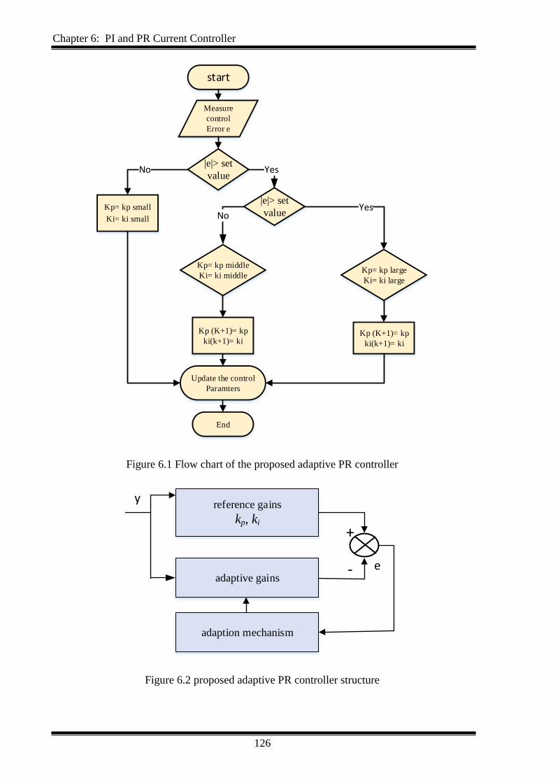
Chapter 6: PI and PR Current Controller
126
Measure
control
Error e
|e|> set
value
start
Yes
Kp= kp large
Ki= ki large
Kp (K+1)= kp
ki(k+1)= ki
Kp= kp middle
Ki= ki middle
Kp (K+1)= kp
ki(k+1)= ki
NoKp= kp small
Ki= ki small
No
End
Update the control
Paramters
Yes|e|> set
value
Figure 6.1 Flow chart of the proposed adaptive PR controller
reference gains
kp, ki
adaptive gains
adaption mechanism
+
- e
y
Figure 6.2 proposed adaptive PR controller structure

Chapter 6: PI and PR Current Controller
127
6.3 Simulation Results of Adaptive PR Controller under
Abnormal Grid Condition
In cases of unbalanced grid conditions, the controller has been tested with different voltage
sags. As a result, the controlled signal starting could promote a rise in the error between the
reference signal, and the controlled signal which can be identified as creating aberration from
its nominal value. To overcome this concern, the adaptive PR control techniques have been
used in the stationary reference frame to control the current based on look-up-table is
implemented to obtain the optimal values of the control parameters. It establishes and associates
the enactment of the adaptive PR controller during standard and irregular grid voltage
conditions.
The performance of the adaptive PR controller has been implemented in abnormal grid
condition. The adaptation mechanism applied allows low PR controller gains until there is a
sudden change in the grid conditions. This means the error will appear eventually. If the error
is less than the set value which is 5%, the adaptation mechanism still used low PR controller
gains. If the error is higher than 5% and less than 8%, the adaptation mechanism will use
medium PR controller gains and the new parameters are applied. If the error is higher than 8%,
the adaptation mechanism will use larger PR controller gains and the new parameters are
applied as can be seen in table Table 6.1. Figure 6.3 shows a screenshot of the adaptive PR
controller in the Simulink.
Table 6.1 Adaptive PR controller simulation parameters
Parameter The proportional gain 𝑘𝑝 The integral gain 𝑘𝑖
α-axis, β-axis current
controllers (low)
1 500
α-axis, β-axis current
controllers (medium)
3 1000
α-axis, β-axis current
controllers (large)
6 1500
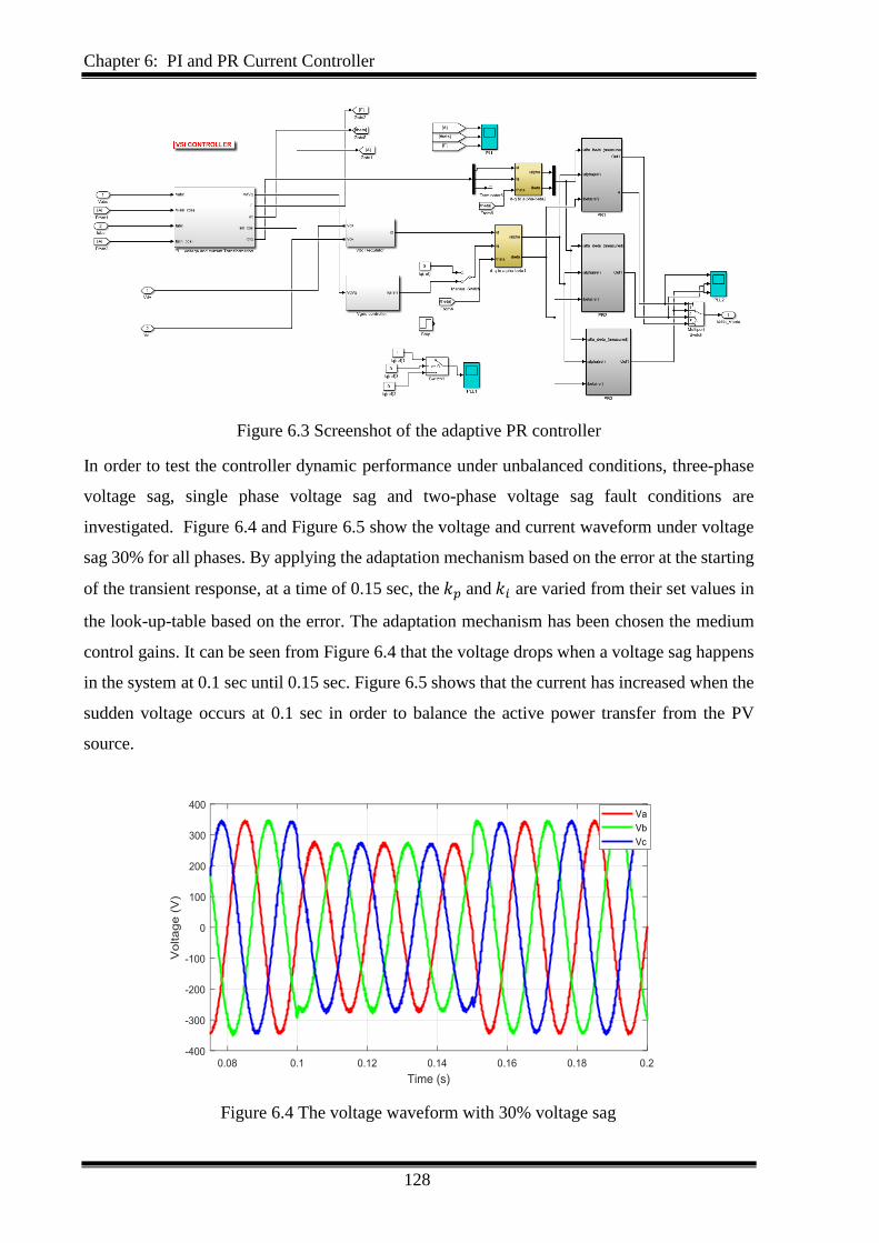
Chapter 6: PI and PR Current Controller
128
Figure 6.3 Screenshot of the adaptive PR controller
In order to test the controller dynamic performance under unbalanced conditions, three-phase
voltage sag, single phase voltage sag and two-phase voltage sag fault conditions are
investigated. Figure 6.4 and Figure 6.5 show the voltage and current waveform under voltage
sag 30% for all phases. By applying the adaptation mechanism based on the error at the starting
of the transient response, at a time of 0.15 sec, the 𝑘𝑝 and 𝑘𝑖 are varied from their set values in
the look-up-table based on the error. The adaptation mechanism has been chosen the medium
control gains. It can be seen from Figure 6.4 that the voltage drops when a voltage sag happens
in the system at 0.1 sec until 0.15 sec. Figure 6.5 shows that the current has increased when the
sudden voltage occurs at 0.1 sec in order to balance the active power transfer from the PV
source.
Figure 6.4 The voltage waveform with 30% voltage sag
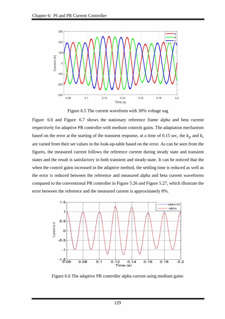
Chapter 6: PI and PR Current Controller
129
Figure 6.5 The current waveform with 30% voltage sag
Figure 6.6 and Figure 6.7 shows the stationary reference frame alpha and beta current
respectively for adaptive PR controller with medium controls gains. The adaptation mechanism
based on the error at the starting of the transient response, at a time of 0.15 sec, the 𝑘𝑝 and 𝑘𝑖
are varied from their set values in the look-up-table based on the error. As can be seen from the
figures, the measured current follows the reference current during steady state and transient
states and the result is satisfactory in both transient and steady-state. It can be noticed that the
when the control gains increased in the adaptive method, the settling time is reduced as well as
the error is reduced between the reference and measured alpha and beta current waveforms
compared to the conventional PR controller in Figure 5.26 and Figure 5.27, which illustrate the
error between the reference and the measured current is approximately 8%.
Figure 6.6 The adaptive PR controller alpha current using medium gains
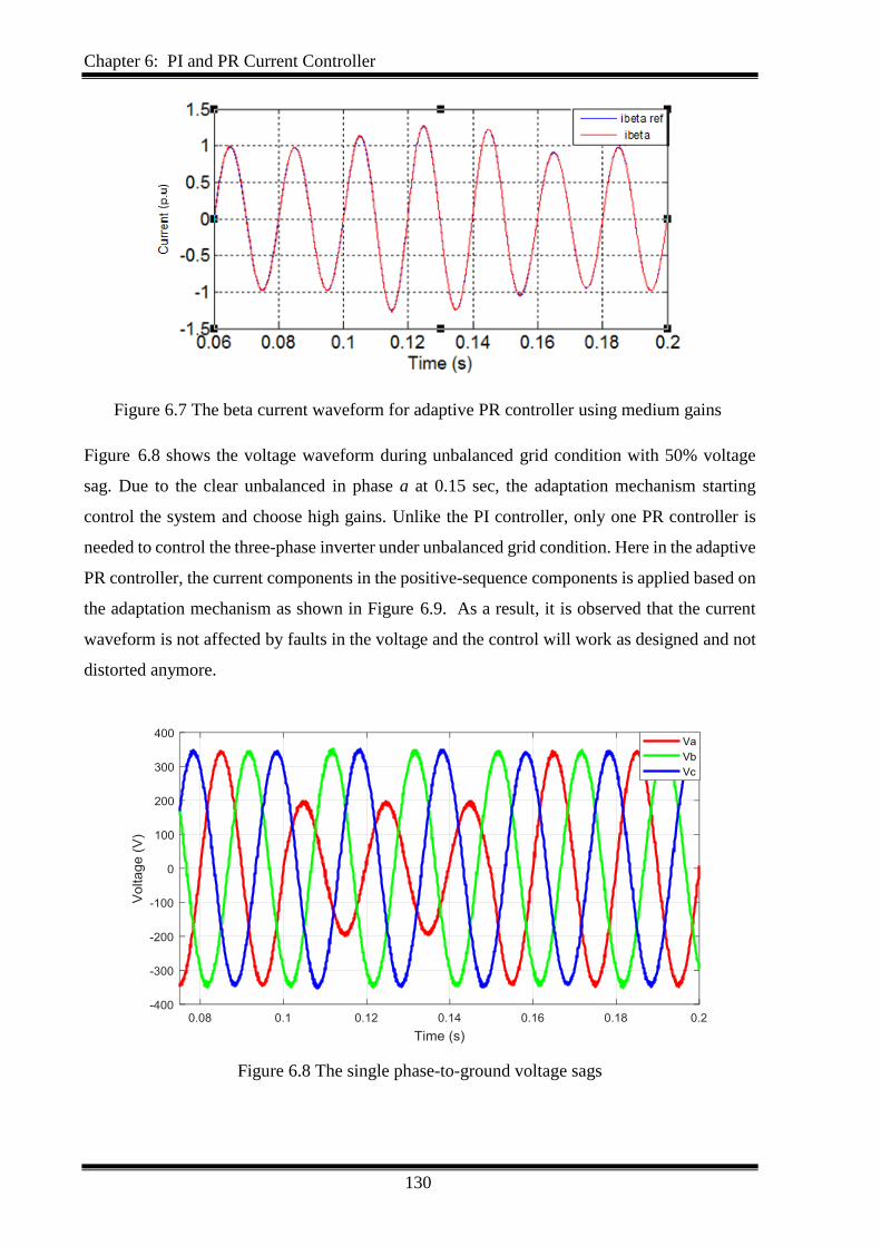
Chapter 6: PI and PR Current Controller
130
Figure 6.7 The beta current waveform for adaptive PR controller using medium gains
Figure 6.8 shows the voltage waveform during unbalanced grid condition with 50% voltage
sag. Due to the clear unbalanced in phase a at 0.15 sec, the adaptation mechanism starting
control the system and choose high gains. Unlike the PI controller, only one PR controller is
needed to control the three-phase inverter under unbalanced grid condition. Here in the adaptive
PR controller, the current components in the positive-sequence components is applied based on
the adaptation mechanism as shown in Figure 6.9. As a result, it is observed that the current
waveform is not affected by faults in the voltage and the control will work as designed and not
distorted anymore.
Figure 6.8 The single phase-to-ground voltage sags
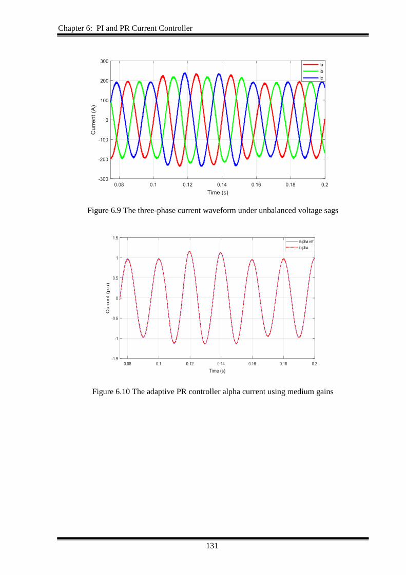
Chapter 6: PI and PR Current Controller
131
Figure 6.9 The three-phase current waveform under unbalanced voltage sags
Figure 6.10 The adaptive PR controller alpha current using medium gains
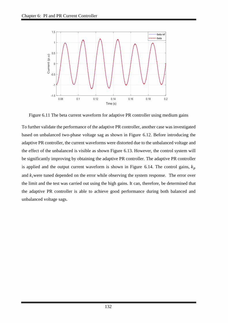
Chapter 6: PI and PR Current Controller
132
Figure 6.11 The beta current waveform for adaptive PR controller using medium gains
To further validate the performance of the adaptive PR controller, another case was investigated
based on unbalanced two-phase voltage sag as shown in Figure 6.12. Before introducing the
adaptive PR controller, the current waveforms were distorted due to the unbalanced voltage and
the effect of the unbalanced is visible as shown Figure 6.13. However, the control system will
be significantly improving by obtaining the adaptive PR controller. The adaptive PR controller
is applied and the output current waveform is shown in Figure 6.14. The control gains, 𝑘𝑝
and 𝑘𝑖were tuned depended on the error while observing the system response. The error over
the limit and the test was carried out using the high gains. It can, therefore, be determined that
the adaptive PR controller is able to achieve good performance during both balanced and
unbalanced voltage sags.
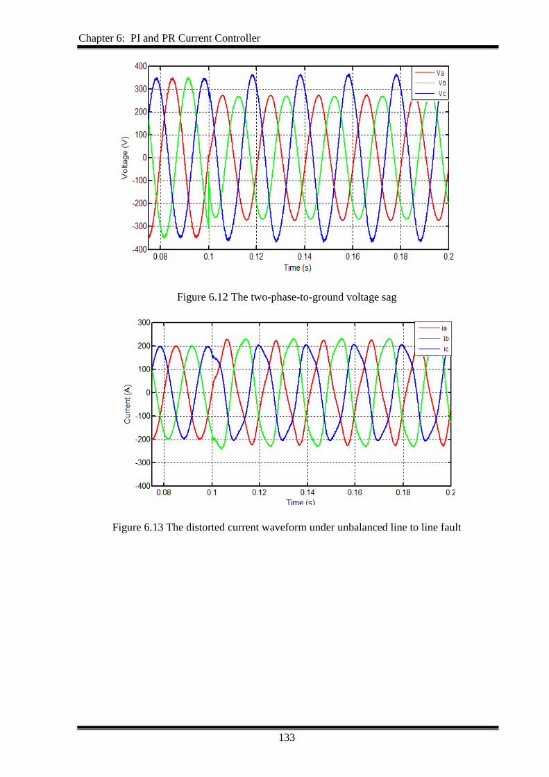
Chapter 6: PI and PR Current Controller
133
Figure 6.12 The two-phase-to-ground voltage sag
Figure 6.13 The distorted current waveform under unbalanced line to line fault
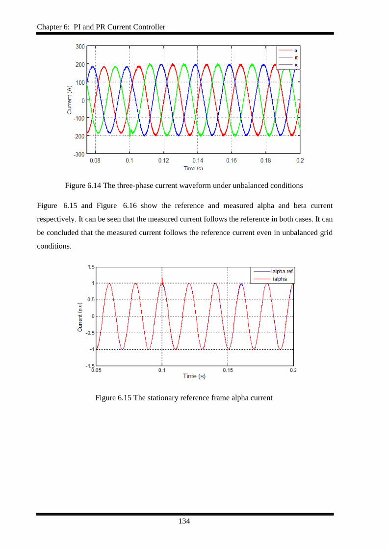
Chapter 6: PI and PR Current Controller
134
Figure 6.14 The three-phase current waveform under unbalanced conditions
Figure 6.15 and Figure 6.16 show the reference and measured alpha and beta current
respectively. It can be seen that the measured current follows the reference in both cases. It can
be concluded that the measured current follows the reference current even in unbalanced grid
conditions.
Figure 6.15 The stationary reference frame alpha current

Chapter 6: PI and PR Current Controller
135
Figure 6.16 The stationary reference frame beta current
6.4 Experimental Results of the Adaptive PR Controller
To validate the control technique for the system in the laboratory, as explained earlier in chapter
5, the system is scaled down and has been tested. The results were obtained under unbalanced
grid conditions such as the line to ground fault voltage sags and line-to-line voltage sags.
Table 6.2 shows the adaptive PR controller parameters. Note, the controller parameters were
adjusted depends on actual values of the adaptation mechanism of the PR controller. This
section is carried out in real-time under different faults conditions using different PR controller
gains according to the system response.
Table 6.2 Adaptive PR controller practical parameters 𝑘𝑝, 𝑘𝑖
Parameter The proportional gain 𝑘𝑝 The integral gain 𝑘𝑖
α-axis, β-axis current controllers
(low)
213 131
α-axis, β-axis current controllers
(medium)
231 219
α-axis, β-axis current controllers
(large)
236 324
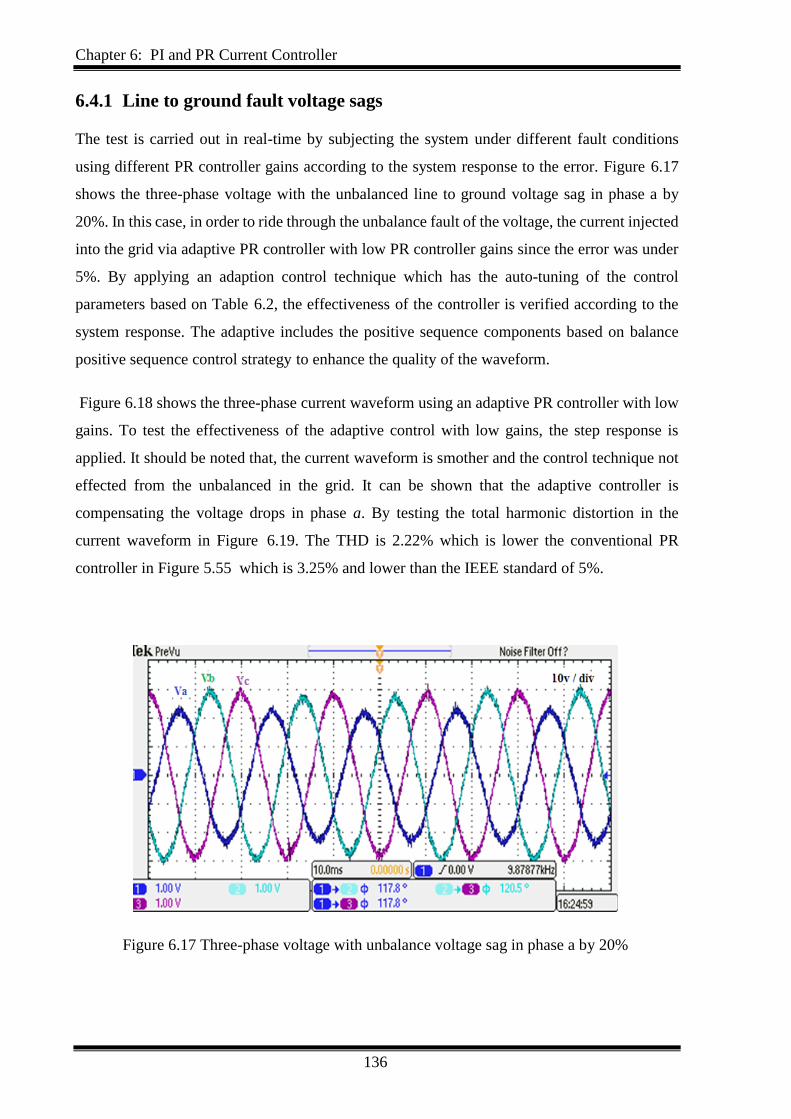
Chapter 6: PI and PR Current Controller
136
6.4.1 Line to ground fault voltage sags
The test is carried out in real-time by subjecting the system under different fault conditions
using different PR controller gains according to the system response to the error. Figure 6.17
shows the three-phase voltage with the unbalanced line to ground voltage sag in phase a by
20%. In this case, in order to ride through the unbalance fault of the voltage, the current injected
into the grid via adaptive PR controller with low PR controller gains since the error was under
5%. By applying an adaption control technique which has the auto-tuning of the control
parameters based on Table 6.2, the effectiveness of the controller is verified according to the
system response. The adaptive includes the positive sequence components based on balance
positive sequence control strategy to enhance the quality of the waveform.
Figure 6.18 shows the three-phase current waveform using an adaptive PR controller with low
gains. To test the effectiveness of the adaptive control with low gains, the step response is
applied. It should be noted that, the current waveform is smother and the control technique not
effected from the unbalanced in the grid. It can be shown that the adaptive controller is
compensating the voltage drops in phase a. By testing the total harmonic distortion in the
current waveform in Figure 6.19. The THD is 2.22% which is lower the conventional PR
controller in Figure 5.55 which is 3.25% and lower than the IEEE standard of 5%.
Figure 6.17 Three-phase voltage with unbalance voltage sag in phase a by 20%
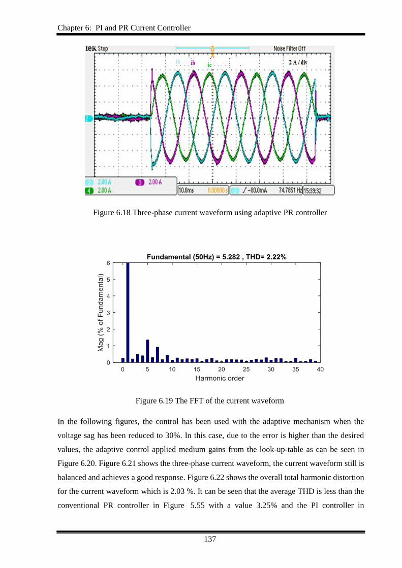
Chapter 6: PI and PR Current Controller
137
Figure 6.18 Three-phase current waveform using adaptive PR controller
Figure 6.19 The FFT of the current waveform
In the following figures, the control has been used with the adaptive mechanism when the
voltage sag has been reduced to 30%. In this case, due to the error is higher than the desired
values, the adaptive control applied medium gains from the look-up-table as can be seen in
Figure 6.20. Figure 6.21 shows the three-phase current waveform, the current waveform still is
balanced and achieves a good response. Figure 6.22 shows the overall total harmonic distortion
for the current waveform which is 2.03 %. It can be seen that the average THD is less than the
conventional PR controller in Figure 5.55 with a value 3.25% and the PI controller in
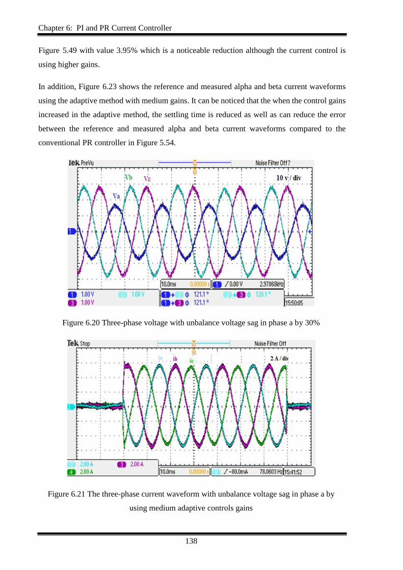
Chapter 6: PI and PR Current Controller
138
Figure 5.49 with value 3.95% which is a noticeable reduction although the current control is
using higher gains.
In addition, Figure 6.23 shows the reference and measured alpha and beta current waveforms
using the adaptive method with medium gains. It can be noticed that the when the control gains
increased in the adaptive method, the settling time is reduced as well as can reduce the error
between the reference and measured alpha and beta current waveforms compared to the
conventional PR controller in Figure 5.54.
Figure 6.20 Three-phase voltage with unbalance voltage sag in phase a by 30%
Figure 6.21 The three-phase current waveform with unbalance voltage sag in phase a by
using medium adaptive controls gains
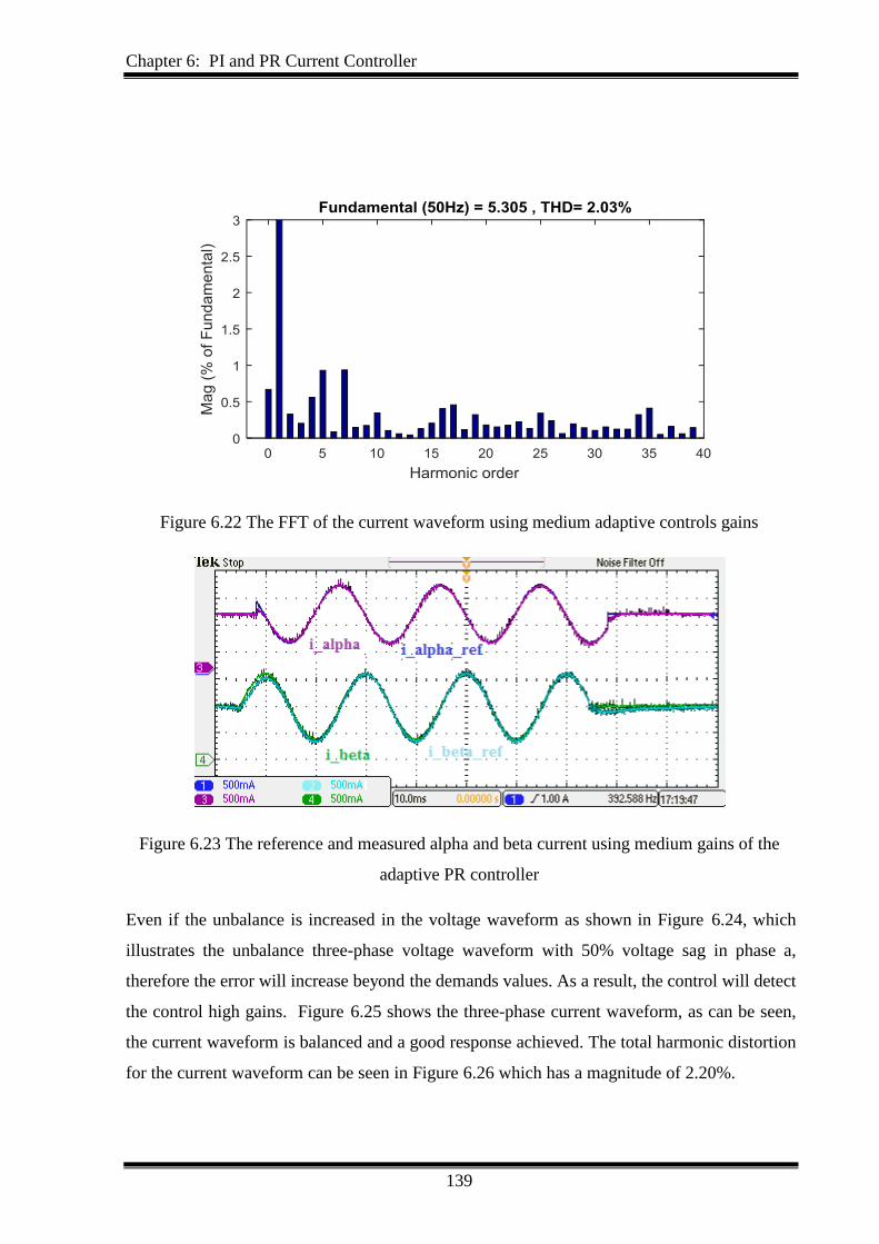
Chapter 6: PI and PR Current Controller
139
Figure 6.22 The FFT of the current waveform using medium adaptive controls gains
Figure 6.23 The reference and measured alpha and beta current using medium gains of the
adaptive PR controller
Even if the unbalance is increased in the voltage waveform as shown in Figure 6.24, which
illustrates the unbalance three-phase voltage waveform with 50% voltage sag in phase a,
therefore the error will increase beyond the demands values. As a result, the control will detect
the control high gains. Figure 6.25 shows the three-phase current waveform, as can be seen,
the current waveform is balanced and a good response achieved. The total harmonic distortion
for the current waveform can be seen in Figure 6.26 which has a magnitude of 2.20%.
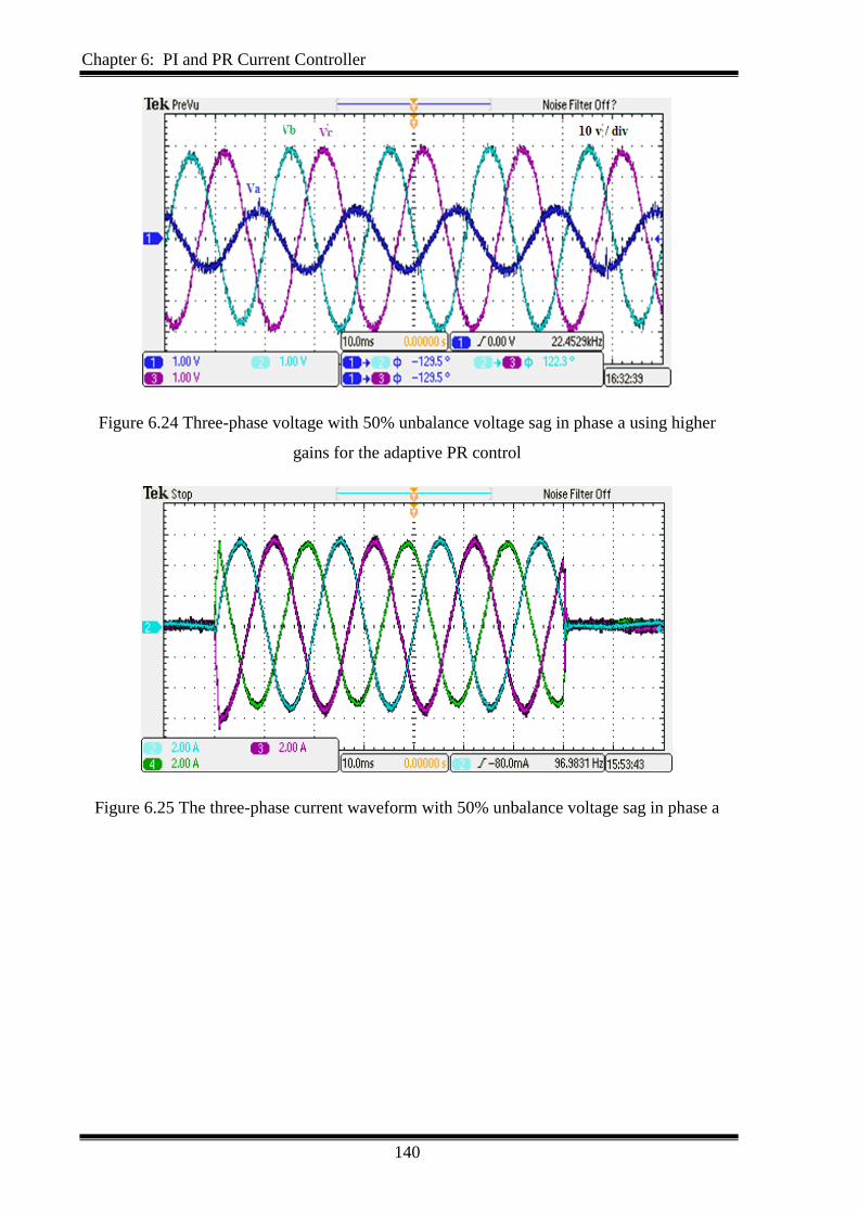
Chapter 6: PI and PR Current Controller
140
Figure 6.24 Three-phase voltage with 50% unbalance voltage sag in phase a using higher
gains for the adaptive PR control
Figure 6.25 The three-phase current waveform with 50% unbalance voltage sag in phase a
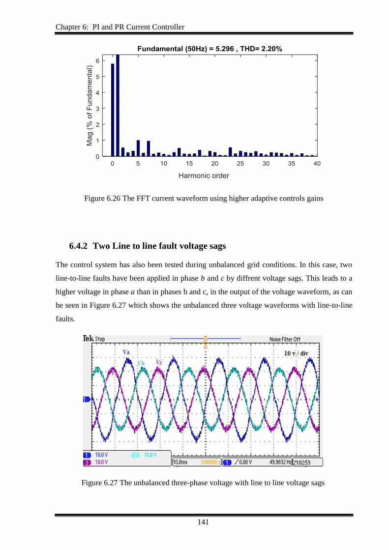
Chapter 6: PI and PR Current Controller
141
Figure 6.26 The FFT current waveform using higher adaptive controls gains
6.4.2 Two Line to line fault voltage sags
The control system has also been tested during unbalanced grid conditions. In this case, two
line-to-line faults have been applied in phase b and c by diffrent voltage sags. This leads to a
higher voltage in phase a than in phases b and c, in the output of the voltage waveform, as can
be seen in Figure 6.27 which shows the unbalanced three voltage waveforms with line-to-line
faults.
Figure 6.27 The unbalanced three-phase voltage with line to line voltage sags
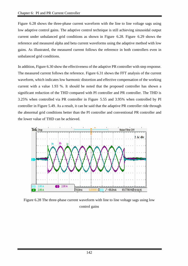
Chapter 6: PI and PR Current Controller
142
Figure 6.28 shows the three-phase current waveform with the line to line voltage sags using
low adaptive control gains. The adaptive control technique is still achieving sinusoidal output
current under unbalanced grid conditions as shown in Figure 6.28. Figure 6.29 shows the
reference and measured alpha and beta current waveforms using the adaptive method with low
gains. As illustrated, the measured current follows the reference in both controllers even in
unbalanced grid conditions.
In addition, Figure 6.30 show the effectiveness of the adaptive PR controller with step response.
The measured current follows the reference. Figure 6.31 shows the FFT analysis of the current
waveform, which indicates low harmonic distortion and effective compensation of the working
current with a value 1.93 %. It should be noted that the proposed controller has shown a
significant reduction of the THD compared with PI controller and PR controller. The THD is
3.25% when controlled via PR controller in Figure 5.55 and 3.95% when controlled by PI
controller in Figure 5.49. As a result, it can be said that the adaptive PR controller ride through
the abnormal grid conditions better than the PI controller and conventional PR controller and
the lower value of THD can be achieved.
Figure 6.28 The three-phase current waveform with line to line voltage sags using low
control gains
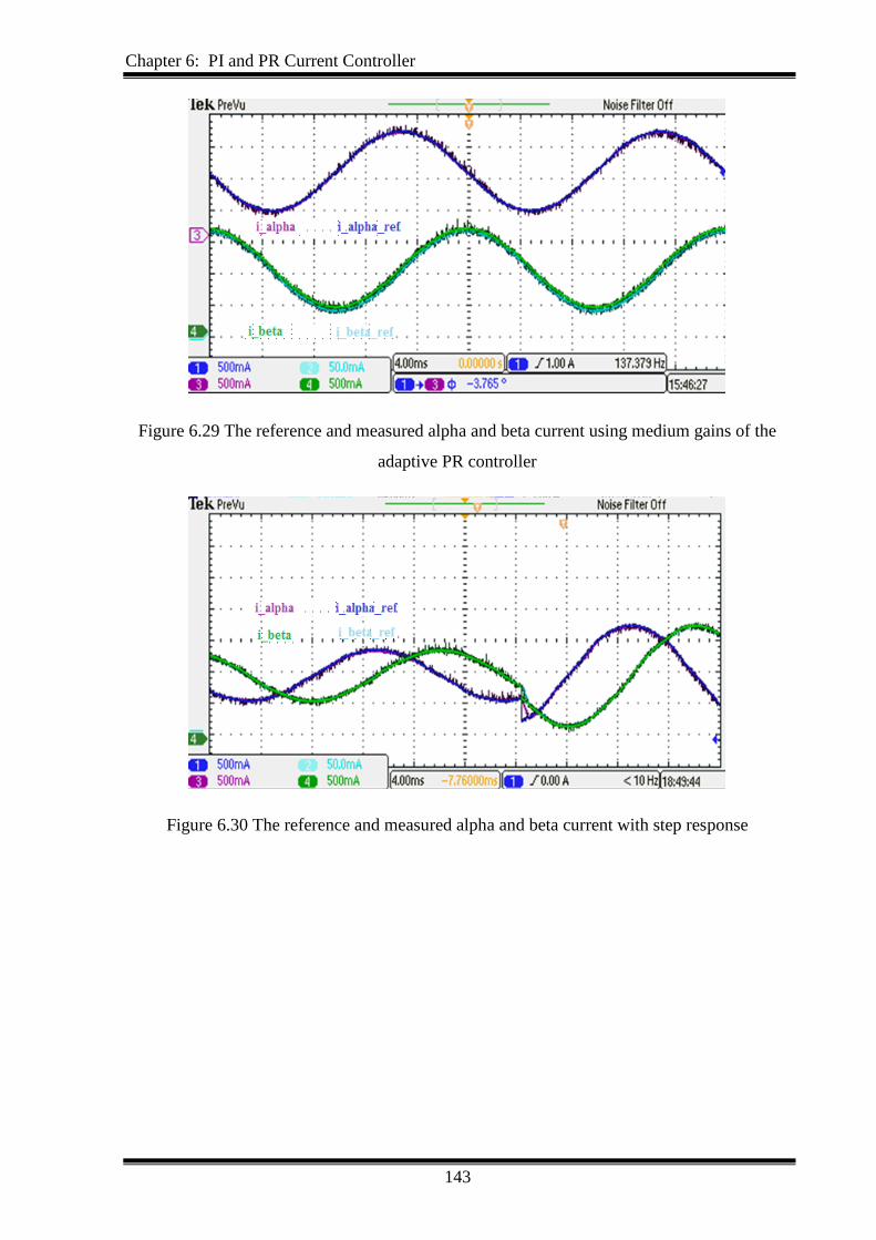
Chapter 6: PI and PR Current Controller
143
Figure 6.29 The reference and measured alpha and beta current using medium gains of the
adaptive PR controller
Figure 6.30 The reference and measured alpha and beta current with step response
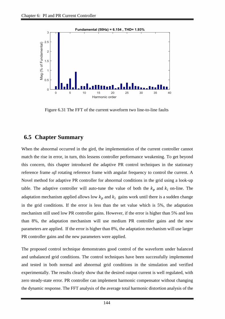
Chapter 6: PI and PR Current Controller
144
Figure 6.31 The FFT of the current waveform two line-to-line faults
6.5 Chapter Summary
When the abnormal occurred in the gird, the implementation of the current controller cannot
match the rise in error, in turn, this lessens controller performance weakening. To get beyond
this concern, this chapter introduced the adaptive PR control techniques in the stationary
reference frame αβ rotating reference frame with angular frequency to control the current. A
Novel method for adaptive PR controller for abnormal conditions in the grid using a look-up
table. The adaptive controller will auto-tune the value of both the 𝑘𝑝 and 𝑘𝑖 on-line. The
adaptation mechanism applied allows low 𝑘𝑝 and 𝑘𝑖 gains work until there is a sudden change
in the grid conditions. If the error is less than the set value which is 5%, the adaptation
mechanism still used low PR controller gains. However, if the error is higher than 5% and less
than 8%, the adaptation mechanism will use medium PR controller gains and the new
parameters are applied. If the error is higher than 8%, the adaptation mechanism will use larger
PR controller gains and the new parameters were applied.
The proposed control technique demonstrates good control of the waveform under balanced
and unbalanced grid conditions. The control techniques have been successfully implemented
and tested in both normal and abnormal grid conditions in the simulation and verified
experimentally. The results clearly show that the desired output current is well regulated, with
zero steady-state error. PR controller can implement harmonic compensator without changing
the dynamic response. The FFT analysis of the average total harmonic distortion analysis of the

Chapter 6: PI and PR Current Controller
145
current waveform indicates are well within acceptable limits and show low harmonic distortion
and effective compensation and less over_shoot of the working current with lower values
compared with the conventional PI and PR controllers.
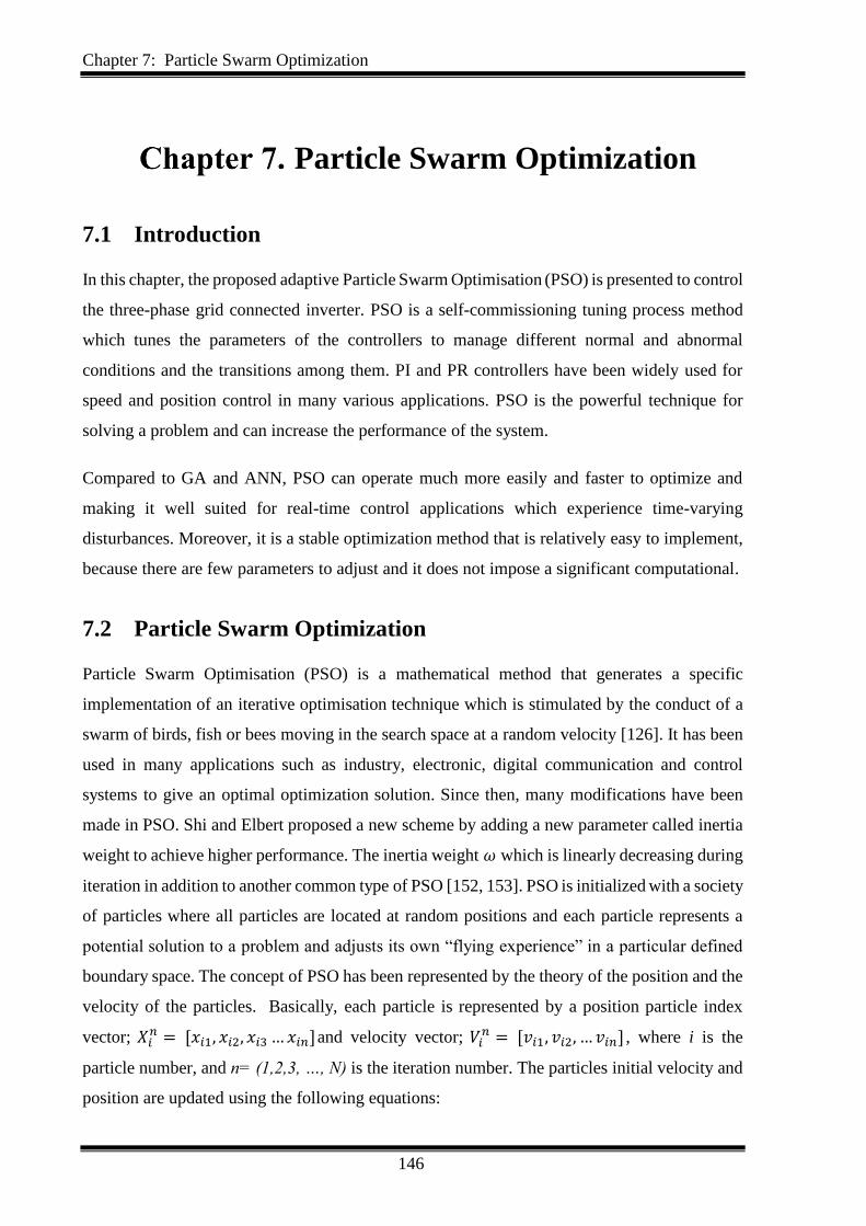
Chapter 7: Particle Swarm Optimization
146
Particle Swarm Optimization
7.1 Introduction
In this chapter, the proposed adaptive Particle Swarm Optimisation (PSO) is presented to control
the three-phase grid connected inverter. PSO is a self-commissioning tuning process method
which tunes the parameters of the controllers to manage different normal and abnormal
conditions and the transitions among them. PI and PR controllers have been widely used for
speed and position control in many various applications. PSO is the powerful technique for
solving a problem and can increase the performance of the system.
Compared to GA and ANN, PSO can operate much more easily and faster to optimize and
making it well suited for real-time control applications which experience time-varying
disturbances. Moreover, it is a stable optimization method that is relatively easy to implement,
because there are few parameters to adjust and it does not impose a significant computational.
7.2 Particle Swarm Optimization
Particle Swarm Optimisation (PSO) is a mathematical method that generates a specific
implementation of an iterative optimisation technique which is stimulated by the conduct of a
swarm of birds, fish or bees moving in the search space at a random velocity [126]. It has been
used in many applications such as industry, electronic, digital communication and control
systems to give an optimal optimization solution. Since then, many modifications have been
made in PSO. Shi and Elbert proposed a new scheme by adding a new parameter called inertia
weight to achieve higher performance. The inertia weight 𝜔 which is linearly decreasing during
iteration in addition to another common type of PSO [152, 153]. PSO is initialized with a society
of particles where all particles are located at random positions and each particle represents a
potential solution to a problem and adjusts its own “flying experience” in a particular defined
boundary space. The concept of PSO has been represented by the theory of the position and the
velocity of the particles. Basically, each particle is represented by a position particle index
vector; 𝑋𝑖𝑛 = [𝑥𝑖1, 𝑥𝑖2, 𝑥𝑖3 …𝑥𝑖𝑛]and velocity vector; 𝑉𝑖
𝑛 = [𝑣𝑖1, 𝑣𝑖2, … 𝑣𝑖𝑛] , where i is the
particle number, and n= (1,2,3, …, N) is the iteration number. The particles initial velocity and
position are updated using the following equations:
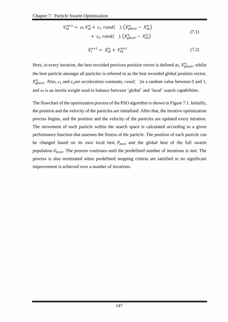
Chapter 7: Particle Swarm Optimization
147
𝑉𝑖𝑑𝑛+1 = 𝜔. 𝑉𝑖𝑑
𝑛 + 𝑐1. 𝑟𝑎𝑛𝑑( ). (𝑋𝑝𝑏𝑒𝑠𝑡𝑛 − 𝑋𝑖𝑑
𝑛 )
+ 𝑐2. 𝑟𝑎𝑛𝑑( ). (𝑋𝑔𝑏𝑒𝑠𝑡𝑛 − 𝑋𝑖𝑑
𝑛 ) (7.1)
𝑋𝑖𝑛+1 = 𝑋𝑖𝑑
𝑛 + 𝑉𝑖𝑑𝑛+1 (7.2)
Here, in every iteration, the best recorded previous position vector is defined as, 𝑋𝑝𝑏𝑒𝑠𝑡𝑛 , whilst
the best particle amongst all particles is referred to as the best recorded global position vector,
𝑋𝑔𝑏𝑒𝑠𝑡𝑛 . Also, 𝑐1 and 𝑐2are acceleration constants, 𝑟𝑎𝑛𝑑( )is a random value between 0 and 1,
and 𝜔 is an inertia weight used to balance between ‘global’ and ‘local’ search capabilities.
The flowchart of the optimization process of the PSO algorithm is shown in Figure 7.1. Initially,
the position and the velocity of the particles are initialised. After that, the iterative optimization
process begins, and the position and the velocity of the particles are updated every iteration.
The movement of each particle within the search space is calculated according to a given
performance function that assesses the fitness of the particle. The position of each particle can
be changed based on its own local best 𝑃𝑏𝑒𝑠𝑡 and the global best of the full swarm
population 𝐺𝑏𝑒𝑠𝑡. The process continues until the predefined number of iterations is met. The
process is also terminated when predefined stopping criteria are satisfied or no significant
improvement is achieved over a number of iterations.
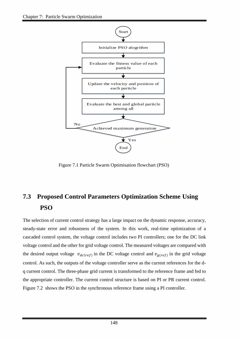
Chapter 7: Particle Swarm Optimization
148
Start
Initialize PSO alogrithm
Evaluate the fitness value of each
particle
Update the velocity and position of
each particle
Evaluate the best and global particle
among all
Achieved maximum generation
End
Yes
No
Figure 7.1 Particle Swarm Optimisation flowchart (PSO)
7.3 Proposed Control Parameters Optimization Scheme Using
PSO
The selection of current control strategy has a large impact on the dynamic response, accuracy,
steady-state error and robustness of the system. In this work, real-time optimization of a
cascaded control system, the voltage control includes two PI controllers; one for the DC link
voltage control and the other for grid voltage control. The measured voltages are compared with
the desired output voltage 𝑣𝑑𝑐(𝑟𝑒𝑓) in the DC voltage control and 𝑣𝑔(𝑟𝑒𝑓) in the grid voltage
control. As such, the outputs of the voltage controller serve as the current references for the d-
q current control. The three-phase grid current is transformed to the reference frame and fed to
the appropriate controller. The current control structure is based on PI or PR current control.
Figure 7.2 shows the PSO in the synchronous reference frame using a PI controller.
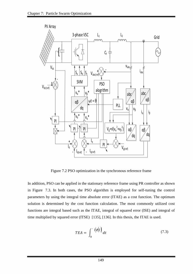
Chapter 7: Particle Swarm Optimization
149
SVM
Sa Sb Sc
αβdq
-
PI PI
abc abc
PLLvα
iα iβvβ
Vdc
-
PI
Vdc(ref)
+
ωt = θ
+
αβαβ
iabc
vabc
vd* vq*
vα* vβ*
-
PV Array
3-phase VSC L1 L2
Cf
Grid
PI
Vg=√(vα2+vβ
2)
Vg(ref)
PSO alogrithm
Vabc(ref)+ -
αβdq
Iq
Id
Id(ref) Iq(ref)
αβdq
Figure 7.2 PSO optimization in the synchronous reference frame
In addition, PSO can be applied in the stationary reference frame using PR controller as shown
in Figure 7.3. In both cases, the PSO algorithm is employed for self-tuning the control
parameters by using the integral time absolute error (ITAE) as a cost function. The optimum
solution is determined by the cost function calculation. The most commonly utilized cost
functions are integral based such as the ITAE, integral of squared error (ISE) and integral of
time multiplied by squared error (ITSE) [135], [136]. In this thesis, the ITAE is used.
𝑇𝐸𝐴 = ∫ tet
𝑑𝑡
0
(7.3)
Chapter 7: Particle Swarm Optimization
150
where e(t) is the difference between the reference and actual values. The cost function is
minimised using equations (7.1) and (7.2) throughout the optimisation process. The block
diagram of the optimization process is shown in Figure 7.4.
SVM
Sa Sb Sc
-
PR
abc abc
PLLvα
iα iβvβ
Vdc
-
PI
Vdc(ref)
+
ωt = θ+
αβαβ
iabc
vabc
iβ*
vα* vβ*
-
PV Array
3-phase VSC L1 L2
Cf
Grid
PI
Vg=√(vα2+vβ
2)
Vg(ref)
PSO alogrithm
Vabc(ref)+ -
αβdq
Iq
IdId(ref) Iq(ref)
αβdq
PR
αβ dq
HC HC
iα*
Figure 7.3 Optimization in the stationary reference frame using PR controller
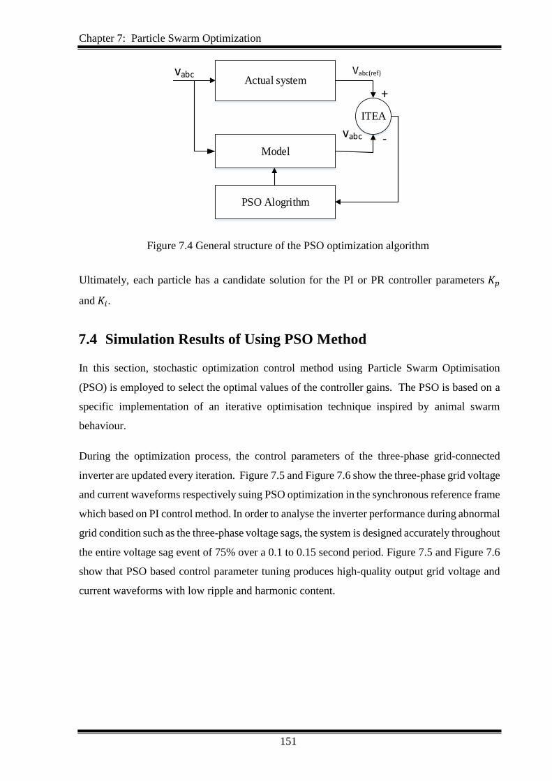
Chapter 7: Particle Swarm Optimization
151
Actual system
Model
PSO Alogrithm
ITEA
+
-
vabc Vabc(ref)
vabc
Figure 7.4 General structure of the PSO optimization algorithm
Ultimately, each particle has a candidate solution for the PI or PR controller parameters 𝐾𝑝
and 𝐾𝑖.
7.4 Simulation Results of Using PSO Method
In this section, stochastic optimization control method using Particle Swarm Optimisation
(PSO) is employed to select the optimal values of the controller gains. The PSO is based on a
specific implementation of an iterative optimisation technique inspired by animal swarm
behaviour.
During the optimization process, the control parameters of the three-phase grid-connected
inverter are updated every iteration. Figure 7.5 and Figure 7.6 show the three-phase grid voltage
and current waveforms respectively suing PSO optimization in the synchronous reference frame
which based on PI control method. In order to analyse the inverter performance during abnormal
grid condition such as the three-phase voltage sags, the system is designed accurately throughout
the entire voltage sag event of 75% over a 0.1 to 0.15 second period. Figure 7.5 and Figure 7.6
show that PSO based control parameter tuning produces high-quality output grid voltage and
current waveforms with low ripple and harmonic content.
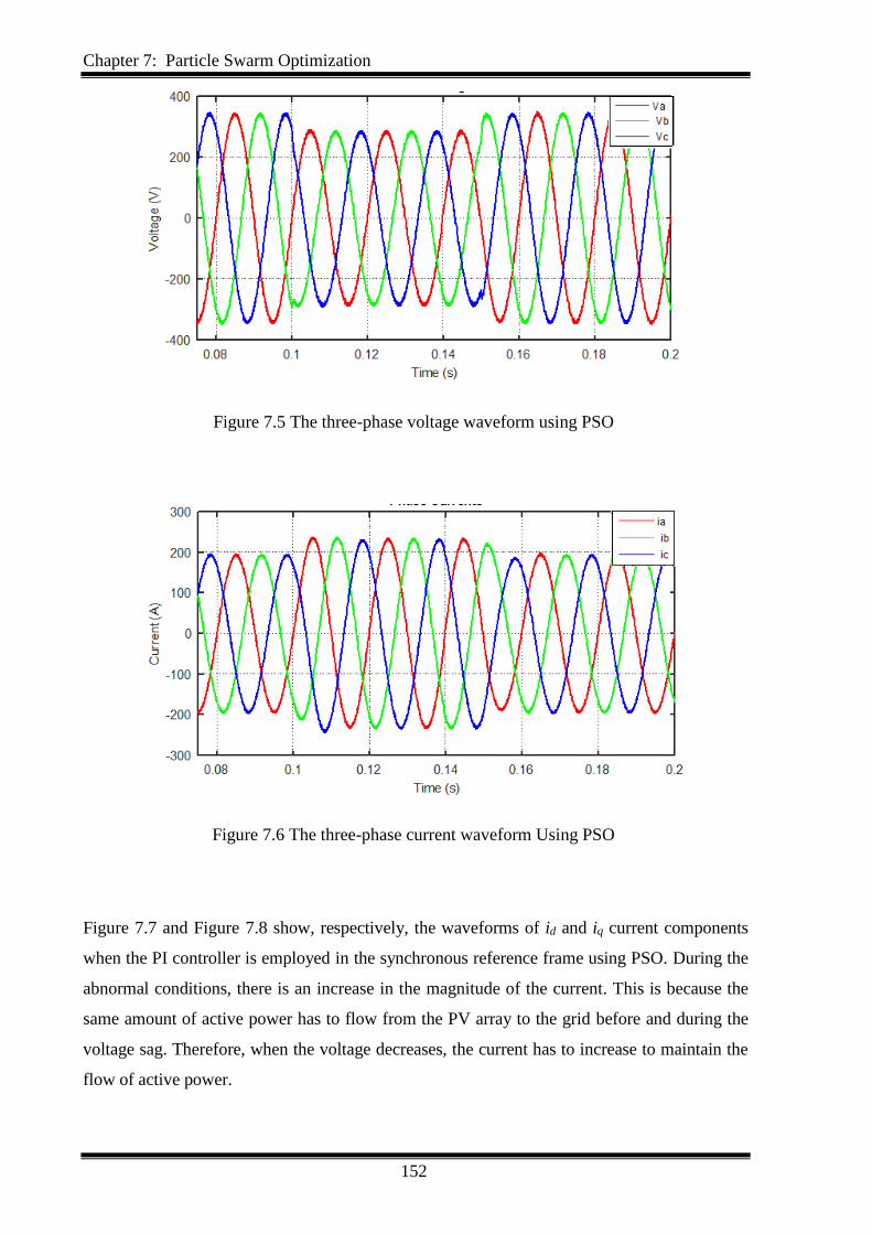
Chapter 7: Particle Swarm Optimization
152
Figure 7.5 The three-phase voltage waveform using PSO
Figure 7.6 The three-phase current waveform Using PSO
Figure 7.7 and Figure 7.8 show, respectively, the waveforms of id and iq current components
when the PI controller is employed in the synchronous reference frame using PSO. During the
abnormal conditions, there is an increase in the magnitude of the current. This is because the
same amount of active power has to flow from the PV array to the grid before and during the
voltage sag. Therefore, when the voltage decreases, the current has to increase to maintain the
flow of active power.
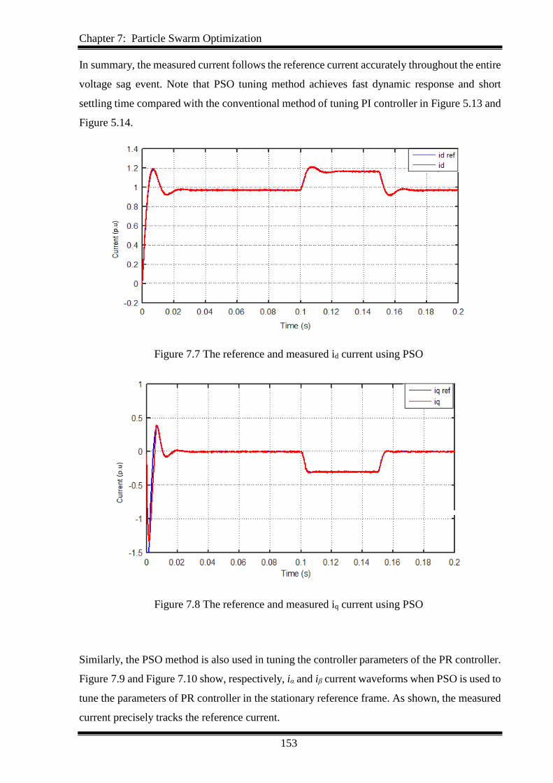
Chapter 7: Particle Swarm Optimization
153
In summary, the measured current follows the reference current accurately throughout the entire
voltage sag event. Note that PSO tuning method achieves fast dynamic response and short
settling time compared with the conventional method of tuning PI controller in Figure 5.13 and
Figure 5.14.
Figure 7.7 The reference and measured id current using PSO
Figure 7.8 The reference and measured iq current using PSO
Similarly, the PSO method is also used in tuning the controller parameters of the PR controller.
Figure 7.9 and Figure 7.10 show, respectively, iα and iβ current waveforms when PSO is used to
tune the parameters of PR controller in the stationary reference frame. As shown, the measured
current precisely tracks the reference current.
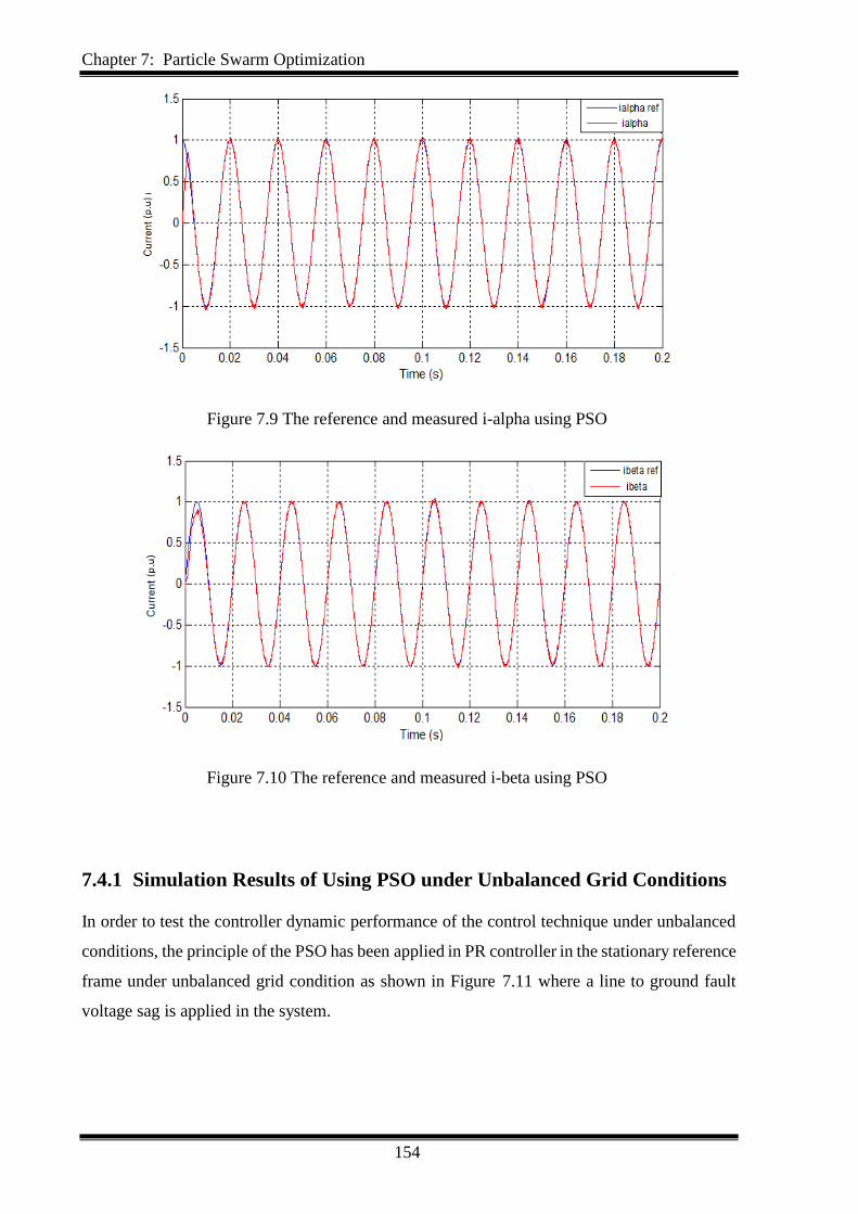
Chapter 7: Particle Swarm Optimization
154
Figure 7.9 The reference and measured i-alpha using PSO
Figure 7.10 The reference and measured i-beta using PSO
7.4.1 Simulation Results of Using PSO under Unbalanced Grid Conditions
In order to test the controller dynamic performance of the control technique under unbalanced
conditions, the principle of the PSO has been applied in PR controller in the stationary reference
frame under unbalanced grid condition as shown in Figure 7.11 where a line to ground fault
voltage sag is applied in the system.
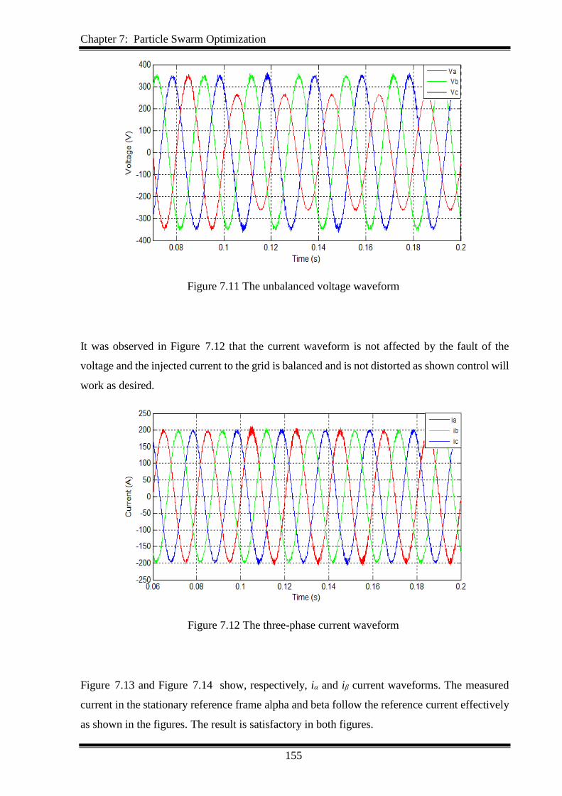
Chapter 7: Particle Swarm Optimization
155
Figure 7.11 The unbalanced voltage waveform
It was observed in Figure 7.12 that the current waveform is not affected by the fault of the
voltage and the injected current to the grid is balanced and is not distorted as shown control will
work as desired.
Figure 7.12 The three-phase current waveform
Figure 7.13 and Figure 7.14 show, respectively, iα and iβ current waveforms. The measured
current in the stationary reference frame alpha and beta follow the reference current effectively
as shown in the figures. The result is satisfactory in both figures.
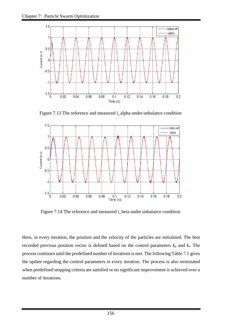
Chapter 7: Particle Swarm Optimization
156
Figure 7.13 The reference and measured i_alpha under unbalance condition
Figure 7.14 The reference and measured i_beta under unbalance condition
Here, in every iteration, the position and the velocity of the particles are initialised. The best
recorded previous position vector is defined based on the control parameters kp and ki. The
process continues until the predefined number of iterations is met. The following Table 7.1 gives
the update regarding the control parameters in every iteration. The process is also terminated
when predefined stopping criteria are satisfied or no significant improvement is achieved over a
number of iterations.
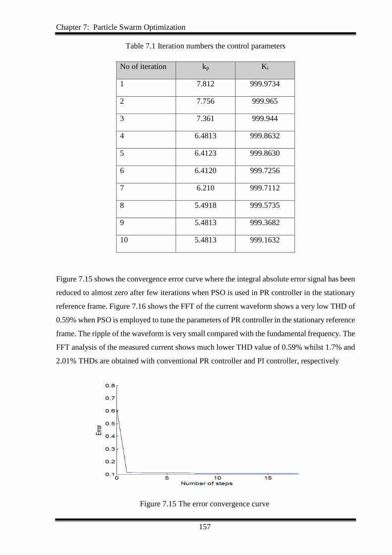
Chapter 7: Particle Swarm Optimization
157
Table 7.1 Iteration numbers the control parameters
No of iteration kp Ki
1 7.812 999.9734
2 7.756 999.965
3 7.361 999.944
4 6.4813 999.8632
5 6.4123 999.8630
6 6.4120 999.7256
7 6.210 999.7112
8 5.4918 999.5735
9 5.4813 999.3682
10 5.4813 999.1632
Figure 7.15 shows the convergence error curve where the integral absolute error signal has been
reduced to almost zero after few iterations when PSO is used in PR controller in the stationary
reference frame. Figure 7.16 shows the FFT of the current waveform shows a very low THD of
0.59% when PSO is employed to tune the parameters of PR controller in the stationary reference
frame. The ripple of the waveform is very small compared with the fundamental frequency. The
FFT analysis of the measured current shows much lower THD value of 0.59% whilst 1.7% and
2.01% THDs are obtained with conventional PR controller and PI controller, respectively
Figure 7.15 The error convergence curve
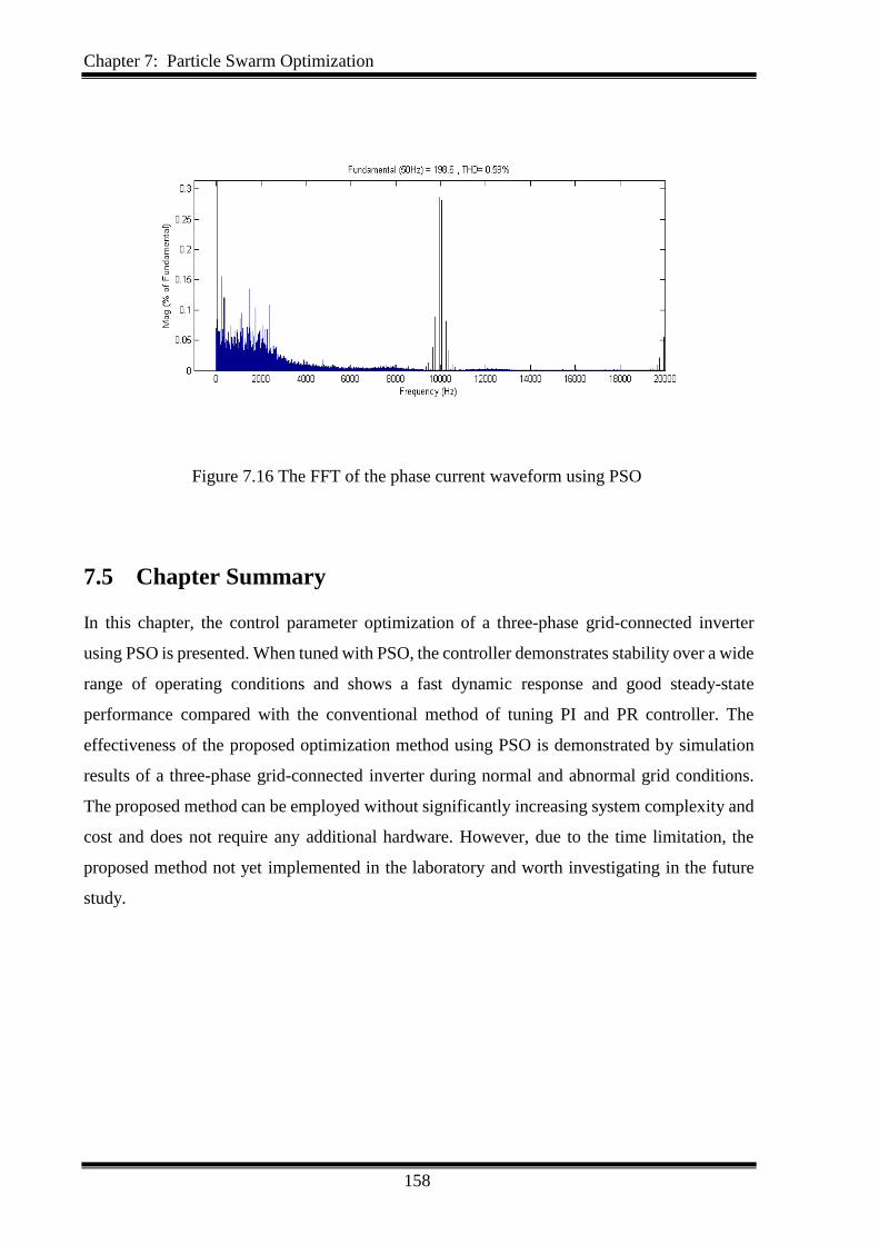
Chapter 7: Particle Swarm Optimization
158
Figure 7.16 The FFT of the phase current waveform using PSO
7.5 Chapter Summary
In this chapter, the control parameter optimization of a three-phase grid-connected inverter
using PSO is presented. When tuned with PSO, the controller demonstrates stability over a wide
range of operating conditions and shows a fast dynamic response and good steady-state
performance compared with the conventional method of tuning PI and PR controller. The
effectiveness of the proposed optimization method using PSO is demonstrated by simulation
results of a three-phase grid-connected inverter during normal and abnormal grid conditions.
The proposed method can be employed without significantly increasing system complexity and
cost and does not require any additional hardware. However, due to the time limitation, the
proposed method not yet implemented in the laboratory and worth investigating in the future
study.
Chapter 8: Conclusion and Future work
159
Conclusion and Future work
8.1 Introduction
It is likely that the aggressive use of non–renewable resources has produced major issues such
as the production of more pollution and greenhouse gas emissions. From this point, researchers
have encouraged organizations to use alternative renewable sources such as photovoltaic and
the wind turbine to generate clean energy.
Photovoltaic, widely abbreviated as solar PV, is a fast growing element of renewable the
market. PV generates DC voltage into appropriate AC voltage for the utility grid via three-
phase grid-connected PV inverter. Three-phase grid-connected PV inverter is connected to the
grid filter to reduce the harmonics inserted into the utility grid. It is aiming to inject the
sinusoidal current intto the utility grid and to be able to deal with any abnormal conditions that
occur in the grid and causes the disturbances through the electric power system.
Thus, these disturbances can be caused in the utility grid by short circuit faults like the line to
ground fault, voltage sags, voltage swell and injected harmonics. This thesis investigated in
detail the influence of the present control scheme of a three-phase grid-connected inverter given
both normal and abnormal grid conditions.
8.2 Conclusion
There are two critical issues in the control of the three-phase inverter connected to the grid
during abnormal condition. Firstly, grid synchronization is required to be more accurate and
should be able to deal with any current controller in the grid-connected inverter. Moreover, this
controller also needs to work perfectly with the symmetrical components of the grid voltage
when the system is unbalanced and proper control of the sequences of both positive and
negative current components injected to the grid is required.
Secondly, depending on the desired performance of the three-phase grid-connected inverter, the
reference current generated by the current controller during abnormal conditions has three status
levels: balanced, unbalanced or distorted and can cause undesired overcurrent tripping.
Although there are many techniques used to control the three-phase grid-connected inverters,
Chapter 8: Conclusion and Future work
160
most of the stake on the same structures which should be taken into account during normal and
abnormal conditions.
In the three-phase grid-connected inverter, current control can be implemented in various ways.
The Proportional Integral current control in the synchronous rotating reference frame dq and
Proportional Resonance current control the stationary reference frame αβ are the most current
control techniques. The implementation of the industrially accepted PI controller, along with
the developing PR controller; accepted in grid-connected renewable energy applications, has
injected the current under abnormal conditions under any circumstance such as grid fault, where
the grid current varies from the normal operating case. Thus, the current control techniques
based on the most suitable strategies that could achieve better results during normal and
abnormal conditions in the thesis are: positive and negative sequence control (PNSC) and
balance positive sequence control (BPSC).
This thesis delivers a straightforward method that decomposes the voltage and current, placing
them into respective positive and negative sequence components that in turn are based on
adaptive delayed filters with one-quarter period deferral. This filter presented in regard to the
adaptive control strategy performance, producing good power quality (unity power factor and
low THD performance) it can only be confirmed through imitation and results based on
experimentation.
In keeping with the claims of other studies, simulation and practical studies have confirmed that
the PR controller shows better performance under normal operating conditions.
The PI current controller indicates good performance and is easy to control. However, it results
in a steady state error which cannot be eliminated when used with sinusoidal references. On the
other hand, the PR controller has the capability to eradicate steady-state error by offering extra
gain at the particular resonant frequency of the controlled signal
The PI controller has lowly functioning connected to cross-coupling between d and q
components of grid current and needs decoupling term between the d and q coordinators and
the voltage feedforward. However, the PR controller is used in the stationary reference frame
α-β coordinates are not cross-coupled and consequently, no decoupling is required. In terms of
the required processing and memory resources, the PI current controller requires additional
mathematical transformation from the stationary reference frame to synchronous reference

Chapter 8: Conclusion and Future work
161
frame. However, with the PR current control Park’s transformation is not needed and hence the
complexity of the control is reduced.
On the other hand, PR controller has the capability to implement harmonic compensator (HC)
in parallel with PR controller without effect the dynamic response of the system and increase
the quality of the quality of the control.
As well as under normal grid conditions, the current controller should be designed to operate
under abnormal grid condition such as short circuit faults, voltage sags, voltage swell. These
faults can be produced by abnormal situations in the grid such as direct starting of large motors,
transformer energizing and capacitor bank charging. During this abnormality, one or more of
phase voltage is reduced or increased than the nominal level at the point of common coupling
(PCC) and causes unbalanced voltage waveform. The unbalanced voltage could be: single
phase to ground faults, two-phase to phase to ground fault and unbalanced three-phase to
ground faults. Therefore, unbalance grid conditions have the most significant impact in terms
of increased current harmonics and ripple in the output power leading to the reductions in power
quality.
To deal with these issues, the current control must be stable as during normal conditions. Under
abnormal operating conditions, a method of the decomposing the voltage and current into its
positive and negative sequence components is usually used. The PI current controller needs to
control both the positive and negative voltage sequence while with the PR controller just the
positive voltage sequence is required reducing the control complexity.
Under abnormal grid conditions, the controlled signal instigating substantial divergence from
its nominal value. The implementation of the orthodox controller cannot remain in line with the
rise in the error accordingly weakening which weakens controller performance. To get beyond
this concern, this shows an enhancement in present-day control using a novel adaptive PR
controller. The adaptive PR control techniques have been used in the stationary reference frame
to control the current. The control techniques have been successfully implemented and tested
in both balanced and unbalanced grid conditions in the simulation and verified experimentally.
The online adaptation is based on a look-up table which is used to update the controller gains.
The proposed control technique is able to provide truncated total harmonic distortion THD in
the injected current even during the occurrence of abnormal grid conditions compared with PI
and PR controllers. The FFT analysis of the measured current shows much lower THD value
Chapter 8: Conclusion and Future work
162
of 1.93% whilst 3.25% and 3.95% THDs are obtained with conventional PR controller and PI
controller, respectively. The proposed method also achieves lower overshoot and settling time
as well as smaller steady-state error. Overall, it can be suggested that the adaptive PR controller
can provide an enhanced output power regulation, thus is better equipped with the result of grid
faults, or procedure in weak grid environments.
Despite the fact that both PI and PR controllers are relatively straightforward to tune, and are
sometimes capable of dealing with many time-varying conditions, most disturbances associated
with grid-connected inverter technology, such as (grid voltage dip or changes in network
impedance) are significantly more challenging and depends on the designer to obtain the best
performance.
This research also presented an adaptive controller tuned using PSO is presented to optimize
the parameters of both PI and PR controllers for the three-phase grid-connected inverter.
Particle Swarm Optimisation is a self-commissioning tuning process method which tunes the
parameters of the controllers to manage different normal and abnormal conditions and the
transitions among them. PSO can operate easily and fast to optimize and is well suited for real-
time control applications which experience time-varying disturbances. It is a stable
optimization method that is relatively easy to implement because there are few parameters to
adjust and it does not impose a significant computational. PSO is a powerful technique for
solving a problem and can enhance the performance of the system.
When tuned with PSO, the controller demonstrated constancy over an expansive range of
operating situations and showed a fast dynamic response and good steady-state performance
compared with conventional methods of tuning PI controller and PR controller. The
effectiveness of the proposed optimization method using PSO is demonstrated by simulation
results of a three-phase grid-connected inverter. The results showed that with PSO parameter
tuning, the current THD is reduced to 0.59% compared to 1.77% when parameters are tuned
with trial and error. The proposed method can be employed without significantly increasing
system complexity and cost and does not require any additional hardware.
8.3 Future Work
This research has investigated the performance of the current control techniques on the three-
phase grid-connected inverter. Although a comprehensive investigation of the impact abnormal
grid conditions, further investigation to take into account the load resistance in the control

Chapter 8: Conclusion and Future work
163
scheme is considered to be worthwhile. Therefore, in continuation of this research, the
following areas might be of interest for further work:
A method of advanced optimization control techniques to control the three-phase grid-
connected application in practical work such as PSO and GA.
PSO can be integrated
The optimization of reactive power sharing control strategies with active power control.
In unbalanced conditions, the voltage control with reactive power compensation. The
other option can be carried out to apply STATCOM system, therefore, bus voltage will
be balanced.
Chapter 8: Conclusion and Future work
164
References
[1] L. Wuhua and H. Xiangning, "Review of Nonisolated High-Step-Up DC/DC Converters in Photovoltaic Grid-Connected Applications," IEEE Trans. Ind Electron., vol. 58, pp. 1239-1250, 2011.
[2] S. B. Kjaer, J. K. Pedersen, and F. Blaabjerg, "A review of single-phase grid-connected inverters for photovoltaic modules," IEEE Transactions on Industry Applications, vol. 41, pp. 1292-1306, 2005.
[3] R. E. P. N. f. t. s. Century, "Renewables 2016 Global Status Report ", (Paris: REN21 Secretariat)2016.
[4] N. Statistics, "Renewable sources of energy: Chapter 6, Digest of United Kingdom Energy Statistics (DUKES)," D. o. E. C. Change, Ed., ed: U.K goverment- Energy Statistics 2015.
[5] I. I. E. Agency, "Snapshot of Global PV Markets," The International Energy Agency (IEA)2015. [6] A. H. Almasoud and H. M. Gandayh, "Future of solar energy in Saudi Arabia," Journal of King
Saud University - Engineering Sciences, vol. 27, pp. 153-157, 2015. [7] SUNPOWER. (6 March). King Abdullah University, Saudi Arabia. Available:
https://global.sunpower.com/solar-case-studies/kaust-saudi-arabia/ [8] T. Yun Tiam and D. S. Kirschen, "Impact on the Power System of a Large Penetration of
Photovoltaic Generation," in Power Engineering Society General Meeting, 2007. IEEE, 2007, pp. 1-8.
[9] T. Stetz, F. Marten, and M. Braun, "Improved Low Voltage Grid-Integration of Photovoltaic Systems in Germany," Sustainable Energy, IEEE Transactions on, vol. 4, pp. 534-542, 2013.
[10] S. Kouro, J. Rodriguez, B. Wu, S. Bernet, and M. Perez, "Powering the Future of Industry: High-Power Adjustable Speed Drive Topologies," IEEE Industry Applications Magazine, vol. 18, pp. 26-39, 2012.
[11] B. Tamyurek, "A High-Performance SPWM Controller for Three-Phase UPS Systems Operating Under Highly Nonlinear Loads," IEEE Transactions on Power Electronics, vol. 28, pp. 3689-3701, 2013.
[12] E. K. Kim, F. Mwasilu, H. H. Choi, and J. W. Jung, "An Observer-Based Optimal Voltage Control Scheme for Three-Phase UPS Systems," IEEE Transactions on Industrial Electronics, vol. 62, pp. 2073-2081, 2015.
[13] P. Rodriguez, J. Pou, J. Bergas, I. Candela, R. Burgos, and D. Boroyevich, "Double Synchronous Reference Frame PLL for Power Converters Control," in Power Electronics Specialists Conference, 2005. PESC '05. IEEE 36th, 2005, pp. 1415-1421.
[14] M. Liserre, F. Blaabjerg, and S. Hansen, "Design and control of an LCL-filter-based three-phase active rectifier," IEEE Trans. Ind App., vol. 41, pp. 1281-1291, 2005.
[15] S. Chakraborty, B. Kramer, and B. Kroposki, "A review of power electronics interfaces for distributed energy systems towards achieving low-cost modular design," Renewable and Sustainable Energy Reviews, vol. 13, pp. 2323-2335, 2009.
[16] T. Kerekes, M. Liserre, R. Teodorescu, C. Klumpner, and M. Sumner, "Evaluation of Three-Phase Transformerless Photovoltaic Inverter Topologies," Power Electronics, IEEE Transactions on, vol. 24, pp. 2202-2211, 2009.
[17] "IEEE Recommended Practice for Utility Interface of Photovoltaic (PV) Systems," IEEE Std 929-2000, p. i, 2000.
[18] "IEEE Recommended Practice for Utility Interface of Residential and Intermediate Photovoltaic (PV) Systems," ANSI/IEEE Std 929-1988, p. 0_1, 1987.
[19] M. A. Elgendy, B. Zahawi, and D. J. Atkinson, "Operating Characteristics of the P&O Algorithm at High Perturbation Frequencies for Standalone PV Systems," IEEE Transactions on Energy Conversion, vol. 30, pp. 189-198, 2015.
[20] R. Kadri, J. P. Gaubert, and G. Champenois, "An Improved Maximum Power Point Tracking for Photovoltaic Grid-Connected Inverter Based on Voltage-Oriented Control," Industrial Electronics, IEEE Transactions on, vol. 58, pp. 66-75, 2011.

Chapter 8: Conclusion and Future work
165
[21] X. Weidong, F. F. Edwin, G. Spagnuolo, and J. Jatskevich, "Efficient Approaches for Modeling and Simulating Photovoltaic Power Systems," Photovoltaics, IEEE Journal of, vol. 3, pp. 500-508, 2013.
[22] J. Rodriguez, S. Bernet, P. K. Steimer, and I. E. Lizama, "A Survey on Neutral-Point-Clamped Inverters," IEEE Transactions on Industrial Electronics, vol. 57, pp. 2219-2230, 2010.
[23] A. Nabae, I. Takahashi, and H. Akagi, "A New Neutral-Point-Clamped PWM Inverter," IEEE Transactions on Industry Applications, vol. IA-17, pp. 518-523, 1981.
[24] B. Xiao, L. Hang, J. Mei, C. Riley, L. M. Tolbert, and B. Ozpineci, "Modular Cascaded H-Bridge Multilevel PV Inverter With Distributed MPPT for Grid-Connected Applications," IEEE Transactions on Industry Applications, vol. 51, pp. 1722-1731, 2015.
[25] F. Wu, X. Li, F. Feng, and H. B. Gooi, "Modified Cascaded Multilevel Grid-Connected Inverter to Enhance European Efficiency and Several Extended Topologies," IEEE Transactions on Industrial Informatics, vol. 11, pp. 1358-1365, 2015.
[26] M. H. Rashid, Power electronics: Circuits, devices & applications, International Edition. United States. : Pearson Education Inc, 2004.
[27] P. Channegowda and V. John, "Filter Optimization for Grid Interactive Voltage Source Inverters," IEEE Transactions on Industrial Electronics, vol. 57, pp. 4106-4114, 2010.
[28] W. Li, X. Ruan, D. Pan, and X. Wang, "Full-Feedforward Schemes of Grid Voltages for a Three-Phase <formula formulatype="inline"> <img src="/images/tex/749.gif" alt="LCL"> </formula>-Type Grid-Connected Inverter," IEEE Transactions on Industrial Electronics, vol. 60, pp. 2237-2250, 2013.
[29] R. Teodorescu, M. Liserre, and P. RodrÃguez, Grid Converters for Photovoltaic and Wind Power Systems: Wiley, 2011.
[30] T. Erika and D. G. Holmes, "Grid current regulation of a three-phase voltage source inverter with an LCL input filter," IEEE Transactions on Power Electronics, vol. 18, pp. 888-895, 2003.
[31] G. Shen, D. Xu, L. Cao, and X. Zhu, "An Improved Control Strategy for Grid-Connected Voltage Source Inverters With an LCL Filter," IEEE Transactions on Power Electronics, vol. 23, pp. 1899-1906, 2008.
[32] F. Liu, Y. Zhou, S. Duan, J. Yin, and B. Liu, "Parameter Design of a Two-Current-Loop Controller Used in a Grid-Connected Inverter System With LCL Filter," IEEE Transactions on Industrial Electronics, vol. 56, pp. 4483-4491, 2009.
[33] M. H. Bierhoff and F. W. Fuchs, "Active Damping for Three-Phase PWM Rectifiers With High-Order Line-Side Filters," IEEE Transactions on Industrial Electronics, vol. 56, pp. 371-379, 2009.
[34] J. Dannehl, F. W. Fuchs, S. Hansen, and P. B. Thogersen, "Investigation of Active Damping Approaches for PI-Based Current Control of Grid-Connected Pulse Width Modulation Converters With LCL Filters," IEEE Transactions on Industry Applications, vol. 46, pp. 1509-1517, 2010.
[35] Rodri, x, P. guez, A. Luna, Mu, x00F, R. S. oz-Aguilar, I. Etxeberria-Otadui, R. Teodorescu, and F. Blaabjerg, "A Stationary Reference Frame Grid Synchronization System for Three-Phase Grid-Connected Power Converters Under Adverse Grid Conditions," IEEE Trans, Power Electron., vol. 27, pp. 99-112, 2012.
[36] F. Mur, V. Cardenas, J. Vaquero, and S. Martinez, "Phase synchronization and measurement digital systems of AC mains for power converters," in Power Electronics Congress, 1998. CIEP 98. VI IEEE International, 1998, pp. 188-194.
[37] J. W. Choi, Y. K. Kim, and H. G. Kim, "Digital PLL control for single-phase photovoltaic system," Electric Power Applications, IEE Proceedings -, vol. 153, pp. 40-46, 2006.
[38] F. M. Gardner, Phaselock Techniques vol. 2nd edition: Wiley-Interscience, 1979. [39] F. Blaabjerg, R. Teodorescu, M. Liserre, and A. V. Timbus, "Overview of Control and Grid
Synchronization for Distributed Power Generation Systems," Industrial Electronics, IEEE Transactions on, vol. 53, pp. 1398-1409, 2006.
[40] H. Guan-Chyun and J. C. Hung, "Phase-locked loop techniques. A survey," IEEE Trans, Ind. Appl., vol. 43, pp. 609-615, 1996.
Chapter 8: Conclusion and Future work
166
[41] A. Timbus, M. Liserre, R. Teodorescu, and F. Blaabjerg, "Synchronization methods for three phase distributed power generation systems - An overview and evaluation," in Power Electronics Specialists Conference, 2005. PESC '05. IEEE 36th, 2005, pp. 2474-2481.
[42] D. Jovcic, "Phase locked loop system for FACTS," IEEE Trans, on Power Systems, vol. 18, pp. 1116-1124, 2003.
[43] M. Weinhold, "A new control for optimal operation of a three-phase voltage dc link PWM converter," in Proc. PCIM Conf 1991, pp. 371-371.
[44] L. A. Serpa, S. Ponnaluri, P. M. Barbosa, and J. W. Kolar, "A Modified Direct Power Control Strategy Allowing the Connection of Three-Phase Inverters to the Grid Through LCL Filters," IEEE Transactions on Industry Applications, vol. 43, pp. 1388-1400, 2007.
[45] N. Alford and J. Fréchet, Proceedings of the Eighth Saudi Students Conference in the UK: World Scientific Publishing Company, 2015.
[46] J. R. Rodriguez, J. W. Dixon, J. R. Espinoza, J. Pontt, and P. Lezana, "PWM regenerative rectifiers: state of the art," IEEE Trans, Ind. Appl., vol. 52, pp. 5-22, 2005.
[47] M. Liserre, F. Blaabjerg, and S. Hansen, "Design and control of an LCL-filter-based three-phase active rectifier," IEEE Trans, Ind. Appl., vol. 41, pp. 1281-1291, 2005.
[48] "IEEE Standard for Interconnecting Distributed Resources With Electric Power Systems," IEEE Std 1547-2003, pp. 0_1-16, 2003.
[49] "Draft Application Guide for IEEE Standard 1547, Interconnecting Distributed Resources with Electric Power Systems," IEEE Unapproved Draft Std P1547.2/D10, Mar 2008, 2008.
[50] M. P. Kazmierkowski and M. A. Dzieniakowski, "Review of current regulation methods for VS-PWM inverters," in Industrial Electronics, 1993. Conference Proceedings, ISIE'93 - Budapest., IEEE International Symposium on, 1993, pp. 448-456.
[51] W. Leonhard, Control of Electrical Drive. Berlin, Germany: Springer-Verlag, 1996. [52] J. Svensson, "Synchronisation methods for grid-connected voltage source converters," IEE
Proceedings - Generation, Transmission and Distribution, vol. 148, pp. 229-235, 2001. [53] K. J. Åström and T. Hägglund, Advanced PID Control: ISA-The Instrumentation, Systems, and
Automation Society, 2006. [54] R. Teodorescu, F. Blaabjerg, U. Borup, and M. Liserre, "A new control structure for grid-
connected LCL PV inverters with zero steady-state error and selective harmonic compensation," in Applied Power Electronics Conference and Exposition, 2004. APEC '04. Nineteenth Annual IEEE, 2004, pp. 580-586 Vol.1.
[55] R. Teodorescu, F. Blaabjerg, M. Liserre, and P. C. Loh, "Proportional-resonant controllers and filters for grid-connected voltage-source converters," IEE Proceedings - Electric Power Applications, vol. 153, pp. 750-762, 2006.
[56] R. Teodorescu and F. Blaabjerg, "Flexible control of small wind turbines with grid failure detection operating in stand-alone and grid-connected mode," IEEE Transactions on Power Electronics, vol. 19, pp. 1323-1332, 2004.
[57] S. Fukuda and T. Yoda, "A novel current-tracking method for active filters based on a sinusoidal internal model [for PWM invertors]," IEEE Transactions on Industry Applications, vol. 37, pp. 888-895, 2001.
[58] S. Byeong-Mun, K. Youngroc, C. Hanju, and L. Hakju, "Current harmonic minimization of a grid-connected photovoltaic 500kW three-phase inverter using PR control," in Energy Conversion Congress and Exposition (ECCE), 2011 IEEE, 2011, pp. 1063-1068.
[59] A. Nicastri and A. Nagliero, "Comparison and evaluation of the PLL techniques for the design of the grid-connected inverter systems," in Industrial Electronics (ISIE), 2010 IEEE International Symposium on, 2010, pp. 3865-3870.
[60] M. Castilla, J. Miret, J. Matas, L. G. de Vicua, and J. M. Guerrero, "Linear Current Control Scheme With Series Resonant Harmonic Compensator for Single-Phase Grid-Connected Photovoltaic Inverters," Industrial Electronics, IEEE Transactions on, vol. 55, pp. 2724-2733, 2008.
Chapter 8: Conclusion and Future work
167
[61] M. Liserre, R. Teodorescu, and F. Blaabjerg, "Multiple harmonics control for three-phase grid converter systems with the use of PI-RES current controller in a rotating frame," Power Electronics, IEEE Transactions on, vol. 21, pp. 836-841, 2006.
[62] R. Teodorescu, F. Blaabjerg, M. Liserre, and P. C. Loh, "Proportional-resonant controllers and filters for grid-connected voltage-source converters," Electric Power Applications, IEE Proceedings, vol. 153, pp. 750-762, 2006.
[63] S. Buso, L. Malesani, and P. Mattavelli, "Comparison of current control techniques for active filter applications," IEEE Transactions on Industrial Electronics, vol. 45, pp. 722-729, 1998.
[64] M. Mohseni and S. M. Islam, "A New Vector-Based Hysteresis Current Control Scheme for Three-Phase PWM Voltage-Source Inverters," IEEE Trans. Power Electron., vol. 25, pp. 2299-2309, 2010.
[65] T. Orłowska-Kowalska, F. Blaabjerg, and J. Rodríguez, Advanced and Intelligent Control in Power Electronics and Drives: Springer International Publishing, 2014.
[66] T. Noguchi, H. Tomiki, S. Kondo, and I. Takahashi, "Direct power control of PWM converter without power-source voltage sensors," IEEE Transactions on Industry Applications, vol. 34, pp. 473-479, 1998.
[67] M. Malinowski, M. P. Kazmierkowski, S. Hansen, F. Blaabjerg, and G. D. Marques, "Virtual-flux-based direct power control of three-phase PWM rectifiers," IEEE Transactions on Industry Applications, vol. 37, pp. 1019-1027, 2001.
[68] R. Wu, S. B. Dewan, and G. R. Slemon, "Analysis of a PWM AC to DC voltage source converter under the predicted current control with a fixed switching frequency," IEEE Transactions on Industry Applications, vol. 27, pp. 756-764, 1991.
[69] Z. Song, W. Chen, and C. Xia, "Predictive Direct Power Control for Three-Phase Grid-Connected Converters Without Sector Information and Voltage Vector Selection," IEEE Transactions on Power Electronics, vol. 29, pp. 5518-5531, 2014.
[70] A. Bouafia, J. P. Gaubert, and F. Krim, "Predictive Direct Power Control of Three-Phase Pulsewidth Modulation (PWM) Rectifier Using Space-Vector Modulation (SVM)," IEEE Transactions on Power Electronics, vol. 25, pp. 228-236, 2010.
[71] M. Castilla, J. Miret, J. L. Sosa, J. Matas, V. de, x00F, and L. G. a, "Grid-Fault Control Scheme for Three-Phase Photovoltaic Inverters With Adjustable Power Quality Characteristics," Power Electronics, IEEE Transactions on, vol. 25, pp. 2930-2940, 2010.
[72] E. E. Juarez and A. Hernandez, "An analytical approach for stochastic assessment of balanced and unbalanced voltage sags in large systems," Power Delivery, IEEE Transactions on, vol. 21, pp. 1493-1500, 2006.
[73] M. Bollen, J. R. Gordon, S. Djokic, K. Stockman, J. Milanovic, R. Neumann, G. Ethier, and F. Zavoda, "Voltage dip immunity of equipment and installations - status and need for further work," in Electricity Distribution (CICED), 2010 China International Conference on, 2010, pp. 1-8.
[74] L. Tzung-Lin, H. Shang-Hung, and C. Yu-Hung, "D-STATCOM With Positive-Sequence Admittance and Negative-Sequence Conductance to Mitigate Voltage Fluctuations in High-Level Penetration of Distributed-Generation Systems," IEEE Trans. Ind. Electron., vol. 60, pp. 1417-1428, 2013.
[75] M. Savaghebi, A. Jalilian, J. C. Vasquez, and J. M. Guerrero, "Autonomous Voltage Unbalance Compensation in an Islanded Droop-Controlled Microgrid," IEEE Trans. Ind. Electron., vol. 60, pp. 1390-1402, 2013.
[76] A. Sannino, J. Svensson, and T. Larsson, "Power-electronic solutions to power quality problems," Electric Power Systems Research, vol. 66, pp. 71-82, 2003.
[77] "IEEE Recommended Practice for Monitoring Electric Power Quality," IEEE Std 1159-1995, p. i, 1995.
[78] F. Salha, F. Colas, and X. Guillaud, "Dynamic performance analysis of a LC-filter grid-connected gas turbine under voltage-sag operation," in Advanced Electromechanical Motion Systems & Electric Drives Joint Symposium, 2009. ELECTROMOTION 2009. 8th International Symposium on, 2009, pp. 1-6.
Chapter 8: Conclusion and Future work
168
[79] J. Miret, M. Castilla, A. Camacho, L. G. d. Vicu, x00F, and J. Matas, "Control Scheme for Photovoltaic Three-Phase Inverters to Minimize Peak Currents During Unbalanced Grid-Voltage Sags," IEEE Transactions on Power Electronics, vol. 27, pp. 4262-4271, 2012.
[80] E. Fuchs and M. A. S. Masoum, Power Quality in Power Systems and Electrical Machines: Elsevier Science, 2011.
[81] L. Chia-Tse, H. Che-Wei, and C. Po-Tai, "A Low-Voltage Ride-Through Technique for Grid-Connected Converters of Distributed Energy Resources," IEEE Trans, Ind. Electron., vol. 47, pp. 1821-1832, 2011.
[82] J. Miret, A. Camacho, M. Castilla, L. G. de Vicuna, and J. Matas, "Control Scheme With Voltage Support Capability for Distributed Generation Inverters Under Voltage Sags," IEEE Trans, Power Electron., vol. 28, pp. 5252-5262, 2013.
[83] A. Camacho, M. Castilla, J. Miret, A. Borrell, and L. Garcia de Vicuna, "Active and Reactive Power Strategies With Peak Current Limitation for Distributed Generation Inverters During Unbalanced Grid Faults," IEEE Trans, Ind. Electron., vol. 62, pp. 1515-1525, 2015.
[84] D. Graovac, V. Katic, and A. Rufer, "Power Quality Problems Compensation With Universal Power Quality Conditioning System," IEEE Trans, Power Del., vol. 22, pp. 968-976, 2007.
[85] F. Barrero, S. Martinez, F. Yeves, F. Mur, and P. M. Martinez, "Universal and reconfigurable to UPS active power filter for line conditioning," IEEE Trans, Power Del., vol. 18, pp. 283-290, 2003.
[86] S. George and V. Agarwal, "A DSP Based Optimal Algorithm for Shunt Active Filter Under Nonsinusoidal Supply and Unbalanced Load Conditions," IEEE Trans, Power Electron., vol. 22, pp. 593-601, 2007.
[87] B. Singh and J. Solanki, "An Implementation of an Adaptive Control Algorithm for a Three-Phase Shunt Active Filter," Industrial Electronics, IEEE Transactions on, vol. 56, pp. 2811-2820, 2009.
[88] W. Fei, J. L. Duarte, and M. A. M. Hendrix, "Grid-Interfacing Converter Systems With Enhanced Voltage Quality for Microgrid Application—Concept and Implementation," IEEE Trans, Power Electron., vol. 26, pp. 3501-3513, 2011.
[89] M. Castilla, J. Miret, A. Camacho, J. Matas, and L. Garcia de Vicuna, "Voltage Support Control Strategies for Static Synchronous Compensators Under Unbalanced Voltage Sags," IEEE Trans, Ind. Electron., vol. 61, pp. 808-820, 2014.
[90] L. Kuang, L. Jinjun, W. Zhaoan, and W. Biao, "Strategies and Operating Point Optimization of STATCOM Control for Voltage Unbalance Mitigation in Three-Phase Three-Wire Systems," IEEE Trans, Power Del., vol. 22, pp. 413-422, 2007.
[91] L. Tzung-Lin, H. Shang-Hung, and C. Yu-Hung, "D-STATCOM With Positive-Sequence Admittance and Negative-Sequence Conductance to Mitigate Voltage Fluctuations in High-Level Penetration of Distributed-Generation Systems," IEEE Trans, Ind. Electron., vol. 60, pp. 1417-1428, 2013.
[92] P. Rodriguez, J. Pou, J. Bergas, J. I. Candela, R. P. Burgos, and D. Boroyevich, "Decoupled Double Synchronous Reference Frame PLL for Power Converters Control," IEEE Transactions on Power Electronics, vol. 22, pp. 584-592, 2007.
[93] H. Awad, J. Svensson, and M. J. Bollen, "Tuning software phase-locked loop for series-connected converters," IEEE Transactions on Power Delivery, vol. 20, pp. 300-308, 2005.
[94] J. Svensson, M. Bongiorno, and A. Sannino, "Practical Implementation of Delayed Signal Cancellation Method for Phase-Sequence Separation," IEEE Transactions on Power Delivery, vol. 22, pp. 18-26, 2007.
[95] V. Kaura and V. Blasko, "Operation of a phase locked loop system under distorted utility conditions," IEEE Transactions on Industry Applications, vol. 33, pp. 58-63, 1997.
[96] C. Se-Kyo, "A phase tracking system for three phase utility interface inverters," IEEE Transactions on Power Electronics, vol. 15, pp. 431-438, 2000.
[97] P. Rodriguez, L. Sainz, and J. Bergas, "Synchronous double reference frame PLL applied to a unified power quality conditioner," in Harmonics and Quality of Power, 2002. 10th International Conference on, 2002, pp. 614-619 vol.2.
Chapter 8: Conclusion and Future work
169
[98] P. Rodriguez, J. Pou, J. Bergas, J. I. Candela, R. P. Burgos, and D. Boroyevich, "Decoupled Double Synchronous Reference Frame PLL for Power Converters Control," Power Electronics, IEEE Transactions on, vol. 22, pp. 584-592, 2007.
[99] L. Kyoung-Jun, L. Jong-Pil, S. Dongsul, Y. Dong-Wook, and K. Hee-Je, "A Novel Grid Synchronization PLL Method Based on Adaptive Low-Pass Notch Filter for Grid-Connected PCS," IEEE Trans, Industrial Electronics, vol. 61, pp. 292-301, 2014.
[100] Y. F. Wang and Y. W. Li, "Analysis and Digital Implementation of Cascaded Delayed-Signal-Cancellation PLL," IEEE Transactions on Power Electronics, vol. 26, pp. 1067-1080, 2011.
[101] H. Geng, D. Xu, and B. Wu, "A Novel Hardware-Based All-Digital Phase-Locked Loop Applied to Grid-Connected Power Converters," IEEE Transactions on Industrial Electronics, vol. 58, pp. 1737-1745, 2011.
[102] P. Rodr, x00Ed, guez, A. Luna, R. S. Mu, x00F, A. oz, I. Etxeberria-Otadui, R. Teodorescu, and F. Blaabjerg, "A Stationary Reference Frame Grid Synchronization System for Three-Phase Grid-Connected Power Converters Under Adverse Grid Conditions," IEEE Transactions on Power Electronics, vol. 27, pp. 99-112, 2012.
[103] Y. Zhou, P. Bauer, J. A. Ferreira, and J. Pierik, "Operation of Grid-Connected DFIG Under Unbalanced Grid Voltage Condition," IEEE Transactions on Energy Conversion, vol. 24, pp. 240-246, 2009.
[104] F. A. S. Neves, M. C. Cavalcanti, H. E. P. de Souza, F. Bradaschia, E. J. Bueno, and M. Rizo, "A Generalized Delayed Signal Cancellation Method for Detecting Fundamental-Frequency Positive-Sequence Three-Phase Signals," Power Delivery, IEEE Transactions on, vol. 25, pp. 1816-1825, 2010.
[105] W. Yi Fei and L. Yun Wei, "Three-Phase Cascaded Delayed Signal Cancellation PLL for Fast Selective Harmonic Detection," Industrial Electronics, IEEE Transactions on, vol. 60, pp. 1452-1463, 2013.
[106] "A New Single-Phase PLL Structure Based on Second Order Generalized Integrator," in Power Electronics Specialists Conference, 2006. PESC '06. 37th IEEE, 2006, pp. 1-6.
[107] A. Kulka, "''Sensorless digital control of grid connected three phase converters for renewable sources'', PhD Thesis," PhD, Norwegian University of Science and Technology, 2009.
[108] J. A. Suul, A. Luna, P. Rodriguez, and T. Undeland, "Voltage-Sensor-Less Synchronization to Unbalanced Grids by Frequency-Adaptive Virtual Flux Estimation," IEEE Transactions on Industrial Electronics, vol. 59, pp. 2910-2923, 2012.
[109] P. Rioual, H. Pouliquen, and J. P. Louis, "Regulation of a PWM rectifier in the unbalanced network state using a generalized model," IEEE Trans, Power Electron., vol. 11, pp. 495-502, 1996.
[110] S. Hong-Seok and N. Kwanghee, "Dual current control scheme for PWM converter under unbalanced input voltage conditions," IEEE Trans, Ind. Electron., vol. 46, pp. 953-959, 1999.
[111] S. Yongsug and T. A. Lipo, "Control scheme in hybrid synchronous stationary frame for PWM AC/DC converter under generalized unbalanced operating conditions," IEEE Transactions on Industry Applications, vol. 42, pp. 825-835, 2006.
[112] I. Etxeberria-Otadui, U. Viscarret, M. Caballero, A. Rufer, and S. Bacha, "New Optimized PWM VSC Control Structures and Strategies Under Unbalanced Voltage Transients," Industrial Electronics, IEEE Transactions on, vol. 54, pp. 2902-2914, 2007.
[113] P. Rodriguez, A. V. Timbus, R. Teodorescu, M. Liserre, and F. Blaabjerg, "Flexible Active Power Control of Distributed Power Generation Systems During Grid Faults," Industrial Electronics, IEEE Transactions on, vol. 54, pp. 2583-2592, 2007.
[114] P. Rodriguez, A. V. Timbus, R. Teodeorescu, M. Liserre, and F. Blaabjerg, "Independent PQ Control for Distributed Power Generation Systems under Grid Faults," in IEEE Industrial Electronics, IECON 2006 - 32nd Annual Conference on, 2006, pp. 5185-5190.
[115] F. Wang, J. L. Duarte, and M. A. M. Hendrix, "Design and analysis of active power control strategies for distributed generation inverters under unbalanced grid faults," Generation, Transmission & Distribution, IET, vol. 4, pp. 905-916, 2010.
Chapter 8: Conclusion and Future work
170
[116] A. V. Timbus, P. Rodriguez, R. Teodorescu, M. Liserre, and F. Blaabjerg, "Control Strategies for Distributed Power Generation Systems Operating on Faulty Grid," in Industrial Electronics, 2006 IEEE International Symposium on, 2006, pp. 1601-1607.
[117] M. Castilla, J. Miret, J. L. Sosa, J. Matas, V. de, x00F, and L. G. a, "Grid-Fault Control Scheme for Three-Phase Photovoltaic Inverters With Adjustable Power Quality Characteristics," IEEE Trans, Power Electron., vol. 25, pp. 2930-2940, 2010.
[118] C. Lascu, L. Asiminoaei, I. Boldea, and F. Blaabjerg, "High Performance Current Controller for Selective Harmonic Compensation in Active Power Filters," IEEE Transactions on Power Electronics, vol. 22, pp. 1826-1835, 2007.
[119] A. Vidal, F. D. Freijedo, A. G. Yepes, P. Fernandez-Comesana, J. Malvar, O. Lopez, and J. Doval-Gandoy, "Assessment and Optimization of the Transient Response of Proportional-Resonant Current Controllers for Distributed Power Generation Systems," Industrial Electronics, IEEE Transactions on, vol. 60, pp. 1367-1383, 2013.
[120] Q. Bi, W.-J. Cai, Q.-G. Wang, C.-C. Hang, L. Eng-Lock, Y. Sun, K.-D. Liu, Y. Zhang, and B. Zou, "Advanced controller auto-tuning and its application in HVAC systems," Control Engineering Practice, vol. 8, pp. 633-644, 2000.
[121] A. Rubaai and P. Young, "EKF-Based PI-/PD-Like Fuzzy-Neural-Network Controller for Brushless Drives," Industry Applications, IEEE Transactions on, vol. 47, pp. 2391-2401, 2011.
[122] A. Rubaai, M. J. Castro-Sitiriche, and A. R. Ofoli, "Design and Implementation of Parallel Fuzzy PID Controller for High-Performance Brushless Motor Drives: An Integrated Environment for Rapid Control Prototyping," Industry Applications, IEEE Transactions on, vol. 44, pp. 1090-1098, 2008.
[123] Y. del Valle, G. K. Venayagamoorthy, S. Mohagheghi, J. C. Hernandez, and R. G. Harley, "Particle Swarm Optimization: Basic Concepts, Variants and Applications in Power Systems," Evolutionary Computation, IEEE Transactions on, vol. 12, pp. 171-195, 2008.
[124] M. S. A. Dahidah, G. Konstantinou, and V. G. Agelidis, "A Review of Multilevel Selective Harmonic Elimination PWM: Formulations, Solving Algorithms, Implementation and Applications," Power Electronics, IEEE Transactions on, vol. 30, pp. 4091-4106, 2015.
[125] J. Vikramarajan, Particle swarm optimizer: Economic dispatch with valve point effect using various Pso techniques. Hamburg: Anchor Acadmic Puplishing, 2014.
[126] J. Kennedy and R. Eberhart, "Particle swarm optimization," in Neural Networks, 1995. Proceedings., IEEE International Conference on, 1995, pp. 1942-1948 vol.4.
[127] S. Yuhui and R. Eberhart, "A modified particle swarm optimizer," in Evolutionary Computation Proceedings, 1998. IEEE World Congress on Computational Intelligence., The 1998 IEEE International Conference on, 1998, pp. 69-73.
[128] J. Robinson and Y. Rahmat-Samii, "Particle swarm optimization in electromagnetics," Antennas and Propagation, IEEE Transactions on, vol. 52, pp. 397-407, 2004.
[129] F. Afshinmanesh, A. Marandi, and M. Shahabadi, "Design of a Single-Feed Dual-Band Dual-Polarized Printed Microstrip Antenna Using a Boolean Particle Swarm Optimization," IEEE Trans. Antennas Propag., vol. 56, pp. 1845-1852, 2008.
[130] L. Lizzi, F. Viani, R. Azaro, and A. Massa, "A PSO-Driven Spline-Based Shaping Approach for Ultrawideband (UWB) Antenna Synthesis," IEEE Trans, Antennas Propag., vol. 56, pp. 2613-2621, 2008.
[131] A. Nagliero, A. Lecci, R. A. Mastromauro, M. Liserre, and A. Dell'Aquila, "Particle Swarm Optimization of a universal inverter," in IECON 2010 - 36th Annual Conference on IEEE Industrial Electronics Society, 2010, pp. 199-204.
[132] W. Al-Saedi, S. W. Lachowicz, and D. Habibi, "An optimal current control strategy for a three-phase grid-connected photovoltaic system using Particle Swarm Optimization," in Power Engineering and Automation Conference (PEAM), 2011 IEEE, 2011, pp. 286-290.
[133] M. Miyatake, M. veerachary, F. Toriumi, N. Fujii, and H. Ko, "Maximum Power Point Tracking of Multiple Photovoltaic Arrays: A PSO Approach," Aerospace and Electronic Systems, IEEE Transactions on, vol. 47, pp. 367-380, 2011.
Chapter 8: Conclusion and Future work
171
[134] C. Il-Yop, L. Wenxin, D. A. Cartes, and K. Schoder, "Control parameter optimization for a microgrid system using particle swarm optimization," in Sustainable Energy Technologies, 2008. ICSET 2008. IEEE International Conference on, 2008, pp. 837-842.
[135] D. Maiti, A. Acharya, M. Chakraborty, A. Konar, and R. Janarthanan, "Tuning PID Controllers using the Integral Time Absolute Error Criterion," in Information and Automation for Sustainability, 2008. ICIAFS 2008. 4th International Conference on, 2008, pp. 457-462.
[136] J. Chao, W. Jing, C. Liulin, and J. Qibing, "Parameters tuning of model free adaptive control based on minimum entropy," Automatica Sinica, IEEE/CAA Journal of, vol. 1, pp. 361-371, 2014.
[137] R. Kadri, J. P. Gaubert, and G. Champenois, "An Improved Maximum Power Point Tracking for Photovoltaic Grid-Connected Inverter Based on Voltage-Oriented Control," IEEE Trans, Ind. Electronic., vol. 58, pp. 66-75, 2011.
[138] J. Holtz, "Pulsewidth modulation for electronic power conversion," Proceedings of the IEEE, vol. 82, pp. 1194-1214, 1994.
[139] J. Holtz, "Pulsewidth modulation-a survey," IEEE Transactions on Industrial Electronics, vol. 39, pp. 410-420, 1992.
[140] Z. Keliang and W. Danwei, "Relationship between space-vector modulation and three-phase carrier-based PWM: a comprehensive analysis [three-phase inverters]," IEEE Transactions on Industrial Electronics, vol. 49, pp. 186-196, 2002.
[141] D. G. Holmes and T. A. Lipo, "Pulse Width Modulation for Power Converters : Principles and Practice," 14 Oct 2003 ed: John Wiley & Sons Inc, 2003, p. 744.
[142] R. Zhang, "High Performance Power Converter System For Nonlinear and Unbalanced Load/Source," PhD, Electrical and Computer Engineering, Virginia Polytechnic Institute and State University, 1998.
[143] L. Hassaine, E. Olias, J. Quintero, and V. Salas, "Overview of power inverter topologies and control structures for grid connected photovoltaic systems," Renewable and Sustainable Energy Reviews, vol. 30, pp. 796-807, 2014.
[144] B. Bahrani, S. Kenzelmann, and A. Rufer, "Multivariable-PI-Based dq Current Control of Voltage Source Converters With Superior Axis Decoupling Capability," Industrial Electronics, IEEE Transactions on, vol. 58, pp. 3016-3026, 2011.
[145] J. Svensson, "Synchronisation methods for grid-connected voltage source converters," Generation, Transmission and Distribution, IEE Proceedings-, vol. 148, pp. 229-235, 2001.
[146] A. Reznik, M. G. Simões, A. Al-Durra, and S. M. Muyeen, "<formula formulatype="inline"><tex Notation="TeX">$LCL$</tex></formula> Filter Design and Performance Analysis for Grid-Interconnected Systems," IEEE Transactions on Industry Applications, vol. 50, pp. 1225-1232, 2014.
[147] K. H. Ahmed, S. J. Finney, and B. W. Williams, "Passive Filter Design for Three-Phase Inverter Interfacing in Distributed Generation," in 2007 Compatibility in Power Electronics, 2007, pp. 1-9.
[148] M. Liserre, F. Blaabjerg, and S. Hansen, "Design and control of an LCL-filter based three-phase active rectifier," in Conference Record of the 2001 IEEE Industry Applications Conference. 36th IAS Annual Meeting (Cat. No.01CH37248), 2001, pp. 299-307 vol.1.
[149] M. Liserre, F. Blaabjerg, and S. Hansen, "Design and control of an LCL-filter-based three-phase active rectifier," IEEE Transactions on Industry Applications, vol. 41, pp. 1281-1291, 2005.
[150] R. Teodorescu and F. Blaabjerg, "Flexible control of small wind turbines with grid failure detection operating in stand-alone and grid-connected mode," Power Electronics, IEEE Transactions on, vol. 19, pp. 1323-1332, 2004.
[151] A. Kiam Heong, G. Chong, and L. Yun, "PID control system analysis, design, and technology," IEEE Transactions on Control Systems Technology, vol. 13, pp. 559-576, 2005.
[152] R. C. Eberhart and Y. Shi, "Comparing inertia weights and constriction factors in particle swarm optimization," in Evolutionary Computation, 2000. Proceedings of the 2000 Congress on, 2000, pp. 84-88 vol.1.

Chapter 8: Conclusion and Future work
172
[153] M. Clerc, "The swarm and the queen: towards a deterministic and adaptive particle swarm optimization," in Evolutionary Computation, 1999. CEC 99. Proceedings of the 1999 Congress on, 1999, p. 1957 Vol. 3.
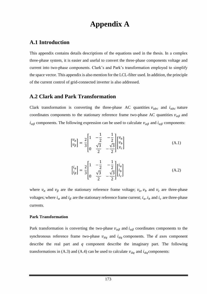
173
Appendix A
A.1 Introduction
This appendix contains details descriptions of the equations used in the thesis. In a complex
three-phase system, it is easier and useful to convert the three-phase components voltage and
current into two-phase components. Clark’s and Park’s transformation employed to simplify
the space vector. This appendix is also mention for the LCL-filter used. In addition, the principle
of the current control of grid-connected inverter is also addressed.
A.2 Clark and Park Transformation
Clark transformation is converting the three-phase AC quantities 𝑣𝑎𝑏𝑐 and 𝑖𝑎𝑏𝑐 nature
coordinates components to the stationary reference frame two-phase AC quantities 𝑣𝛼𝛽 and
𝑖𝛼𝛽 components. The following expression can be used to calculate 𝑣𝛼𝛽 and 𝑖𝛼𝛽 components:
[𝑣𝛼
𝑣𝛽] =
2
3[ 1 −
1
2−
1
2
0√3
2−
√3
2 ]
[
𝑣𝑎
𝑣𝑏
𝑣𝑐
] (A.1)
[𝑖𝛼𝑖𝛽
] = 2
3[ 1 −
1
2−
1
2
0√3
2−
√3
2 ]
[𝑖𝑎𝑖𝑏𝑖𝑐
] (A.2)
where 𝑣𝛼 and 𝑣𝛽 are the stationary reference frame voltage; 𝑣𝑎 , 𝑣𝑏 and 𝑣𝑐 are three-phase
voltages; where 𝑖𝛼 and 𝑖𝛽 are the stationary reference frame current; 𝑖𝑎, 𝑖𝑏 and 𝑖𝑐 are three-phase
currents.
Park Transformation
Park transformation is converting the two-phase 𝑣𝛼𝛽 and 𝑖𝛼𝛽 coordinates components to the
synchronous reference frame two-phase 𝑣𝑑𝑞 and 𝑖𝑑𝑞 components. The 𝑑 axes component
describe the real part and 𝑞 component describe the imaginary part. The following
transformations in (A.3) and (A.4) can be used to calculate 𝑣𝑑𝑞 and 𝑖𝑑𝑞components:
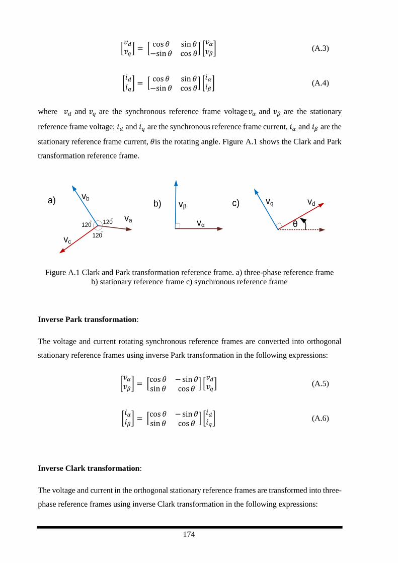
174
[𝑣𝑑
𝑣𝑞] = [
cos 𝜃 sin 𝜃−sin 𝜃 cos 𝜃
] [𝑣𝛼
𝑣𝛽] (A.3)
[𝑖𝑑𝑖𝑞
] = [cos 𝜃 sin 𝜃−sin 𝜃 cos 𝜃
] [𝑖𝛼𝑖𝛽
] (A.4)
where 𝑣𝑑 and 𝑣𝑞 are the synchronous reference frame voltage𝑣𝛼 and 𝑣𝛽 are the stationary
reference frame voltage; 𝑖𝑑 and 𝑖𝑞 are the synchronous reference frame current, 𝑖𝛼 and 𝑖𝛽 are the
stationary reference frame current, 𝜃is the rotating angle. Figure A.1 shows the Clark and Park
transformation reference frame.
va
vb
vc
120
120
120
a) vdvqc)b)
vα
vβ
θ
Figure A.1 Clark and Park transformation reference frame. a) three-phase reference frame
b) stationary reference frame c) synchronous reference frame
Inverse Park transformation:
The voltage and current rotating synchronous reference frames are converted into orthogonal
stationary reference frames using inverse Park transformation in the following expressions:
[𝑣𝛼
𝑣𝛽] = [
cos 𝜃 − sin 𝜃sin 𝜃 cos 𝜃
] [𝑣𝑑
𝑣𝑞] (A.5)
[𝑖𝛼𝑖𝛽
] = [cos 𝜃 − sin 𝜃sin 𝜃 cos 𝜃
] [𝑖𝑑𝑖𝑞
] (A.6)
Inverse Clark transformation:
The voltage and current in the orthogonal stationary reference frames are transformed into three-
phase reference frames using inverse Clark transformation in the following expressions:

175
[
𝑣𝑎
𝑣𝑏
𝑣𝑐
] =
[
1 0
−1
2
√3
2
−1
2−
√3
2 ]
[𝑣𝛼
𝑣𝛽] (A.7)
[𝑖𝑎𝑖𝑏𝑖𝑐
] =
[
1 0
−1
2
√3
2
−1
2−
√3
2 ]
[𝑖𝛼𝑖𝛽
] (A.8)
The previous state expressions using Park’s transformation can be used in the design of LCL
filter.
A.3 LCL Filter Mathematical Model:
The LCL-filter in the Figure A.2 can be described in the following matrix expression based on
rotating frames d axis and q axis at rotating speed 𝜔
- -
ea
+
Vdc
Grid
a
b
c
+
+
-
Vdc/2
Vdc/2
N
S1
S2
S3
S4
S5
S6
L1 L2+ igR1 R2+Rg
+
L1L2
+
igR1+
L1L2 igR1
+
Vc Vc Vc
ea
eb
ec
ia
ib
ic
+ R2+Rg
R2+Rg
Figure A.2 Three-phase grid-connected inverter
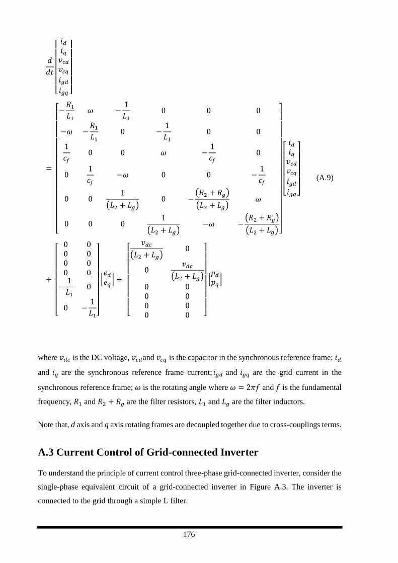
176
𝑑
𝑑𝑡
[ 𝑖𝑑𝑖𝑞𝑣𝑐𝑑
𝑣𝑐𝑞
𝑖𝑔𝑑
𝑖𝑔𝑞 ]
=
[ −
𝑅1
𝐿1𝜔 −
1
𝐿10 0 0
−𝜔 −𝑅1
𝐿10 −
1
𝐿10 0
1
𝑐𝑓0 0 𝜔 −
1
𝑐𝑓0
01
𝑐𝑓−𝜔 0 0 −
1
𝑐𝑓
0 01
(𝐿2 + 𝐿𝑔)0 −
(𝑅2 + 𝑅𝑔)
(𝐿2 + 𝐿𝑔)𝜔
0 0 01
(𝐿2 + 𝐿𝑔)−𝜔 −
(𝑅2 + 𝑅𝑔)
(𝐿2 + 𝐿𝑔)]
[ 𝑖𝑑𝑖𝑞𝑣𝑐𝑑
𝑣𝑐𝑞
𝑖𝑔𝑑
𝑖𝑔𝑞 ]
+
[
0 00 00 00 0
−1
𝐿10
0 −1
𝐿1]
[𝑒𝑑
𝑒𝑞] +
[
𝑣𝑑𝑐
(𝐿2 + 𝐿𝑔)0
0𝑣𝑑𝑐
(𝐿2 + 𝐿𝑔)
0 00 00 00 0 ]
[𝑝𝑑
𝑝𝑞]
(A.9)
where 𝑣𝑑𝑐 is the DC voltage, 𝑣𝑐𝑑and 𝑣𝑐𝑞 is the capacitor in the synchronous reference frame; 𝑖𝑑
and 𝑖𝑞 are the synchronous reference frame current; 𝑖𝑔𝑑 and 𝑖𝑔𝑞 are the grid current in the
synchronous reference frame; 𝜔 is the rotating angle where 𝜔 = 2𝜋𝑓 and 𝑓 is the fundamental
frequency, 𝑅1 and 𝑅2 + 𝑅𝑔 are the filter resistors, 𝐿1 and 𝐿𝑔 are the filter inductors.
Note that, d axis and q axis rotating frames are decoupled together due to cross-couplings terms.
A.3 Current Control of Grid-connected Inverter
To understand the principle of current control three-phase grid-connected inverter, consider the
single-phase equivalent circuit of a grid-connected inverter in Figure A.3. The inverter is
connected to the grid through a simple L filter.
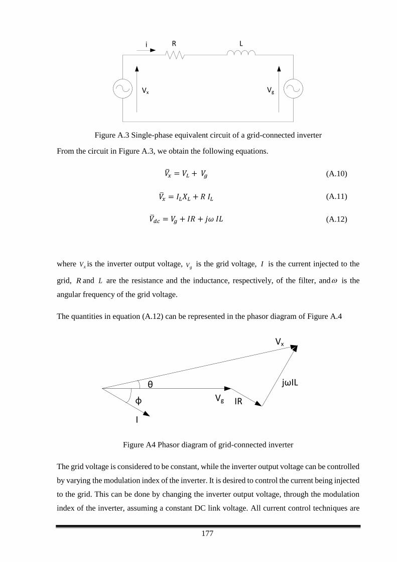
177
Vx Vg
i R L
Figure A.3 Single-phase equivalent circuit of a grid-connected inverter
From the circuit in Figure A.3, we obtain the following equations.
𝑥 = 𝑉𝐿 + 𝑉𝑔 (A.10)
𝑥 = 𝐼𝐿𝑋𝐿 + 𝑅 𝐼𝐿 (A.11)
𝑑𝑐 = 𝑉𝑔 + 𝐼𝑅 + 𝑗𝜔 𝐼𝐿 (A.12)
where xV is the inverter output voltage, gV is the grid voltage, I is the current injected to the
grid, R and L are the resistance and the inductance, respectively, of the filter, and is the
angular frequency of the grid voltage.
The quantities in equation (A.12) can be represented in the phasor diagram of Figure A.4
Vg
Vx
I
IR
jωIL
φ
θ
Figure A4 Phasor diagram of grid-connected inverter
The grid voltage is considered to be constant, while the inverter output voltage can be controlled
by varying the modulation index of the inverter. It is desired to control the current being injected
to the grid. This can be done by changing the inverter output voltage, through the modulation
index of the inverter, assuming a constant DC link voltage. All current control techniques are
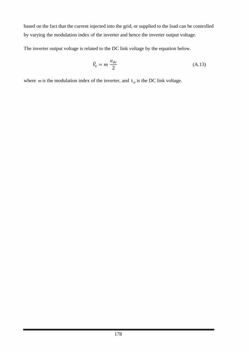
178
based on the fact that the current injected into the grid, or supplied to the load can be controlled
by varying the modulation index of the inverter and hence the inverter output voltage.
The inverter output voltage is related to the DC link voltage by the equation below.
𝑥 = 𝑚 𝑣𝑑𝑐
2 (A.13)
where m is the modulation index of the inverter, and dcV is the DC link voltage.
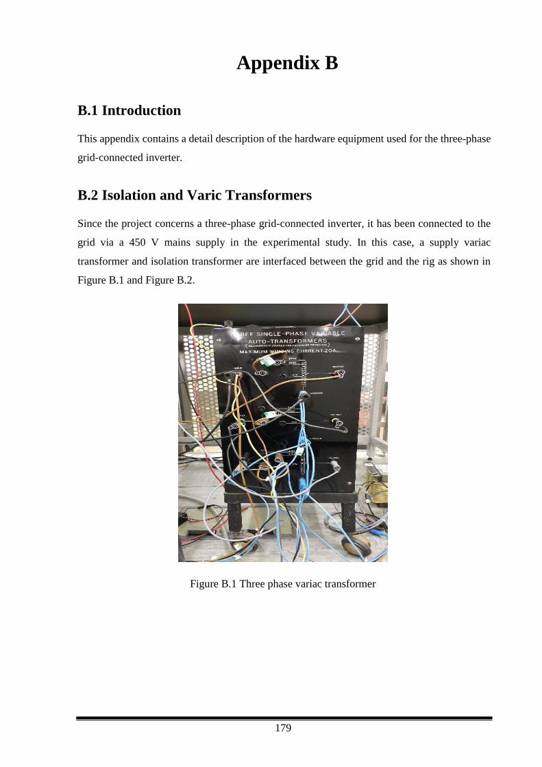
179
Appendix B
B.1 Introduction
This appendix contains a detail description of the hardware equipment used for the three-phase
grid-connected inverter.
B.2 Isolation and Varic Transformers
Since the project concerns a three-phase grid-connected inverter, it has been connected to the
grid via a 450 V mains supply in the experimental study. In this case, a supply variac
transformer and isolation transformer are interfaced between the grid and the rig as shown in
Figure B.1 and Figure B.2.
Figure B.1 Three phase variac transformer

180
Figure B.2 Three phase isolation transformer
The three-phase variac transformer is used in order to effectively regulate the voltage from the
mains supply to the experimental grid-connected PV inverter system. In addition, it allows the
DC link voltage to be used at low values instead of using the conversion ratio between DC/AC
applications. However, the variac is a non-isolated transformer which has no protection from
any feedback of the DC current into the mains supply. Thus, to overcome this issue, an isolation
transformer is connected between the grid’s mains supply and the variac transformer. The
connection is Δ-Y as shown in
In addition, Figure B.3 shows the LCL filter connected the rig. An LCL filter has been used in
the experiment to smoothe the output waveform from the AC side of the inverter and thus
reduce the harmonic of the switching frequency.
Two three-phase inductances are tapped to five different readings in order to test the effect of
various values of inductances. TheL1 , tapped from 0.3mh to 0.8mh andL2 , tapped from
0.1mh to 0.3mh with a rating current of 15A. Different values of inductances and
capacitances have been tested and the most suitable values chosen for a 10 KHz switching
frequency.
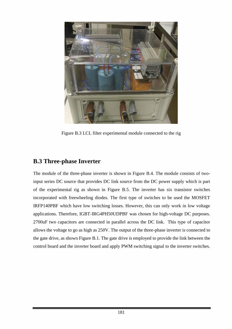
181
Figure B.3 LCL filter experimental module connected to the rig
B.3 Three-phase Inverter
The module of the three-phase inverter is shown in Figure B.4. The module consists of two-
input series DC source that provides DC link source from the DC power supply which is part
of the experimental rig as shown in Figure B.5. The inverter has six transistor switches
incorporated with freewheeling diodes. The first type of switches to be used the MOSFET
IRFP140PBF which have low switching losses. However, this can only work in low voltage
applications. Therefore, IGBT-IRG4PH50UDPBF was chosen for high-voltage DC purposes.
2700uF two capacitors are connected in parallel across the DC link. This type of capacitor
allows the voltage to go as high as 250V. The output of the three-phase inverter is connected to
the gate drive, as shown Figure B.1. The gate drive is employed to provide the link between the
control board and the inverter board and apply PWM switching signal to the inverter switches.
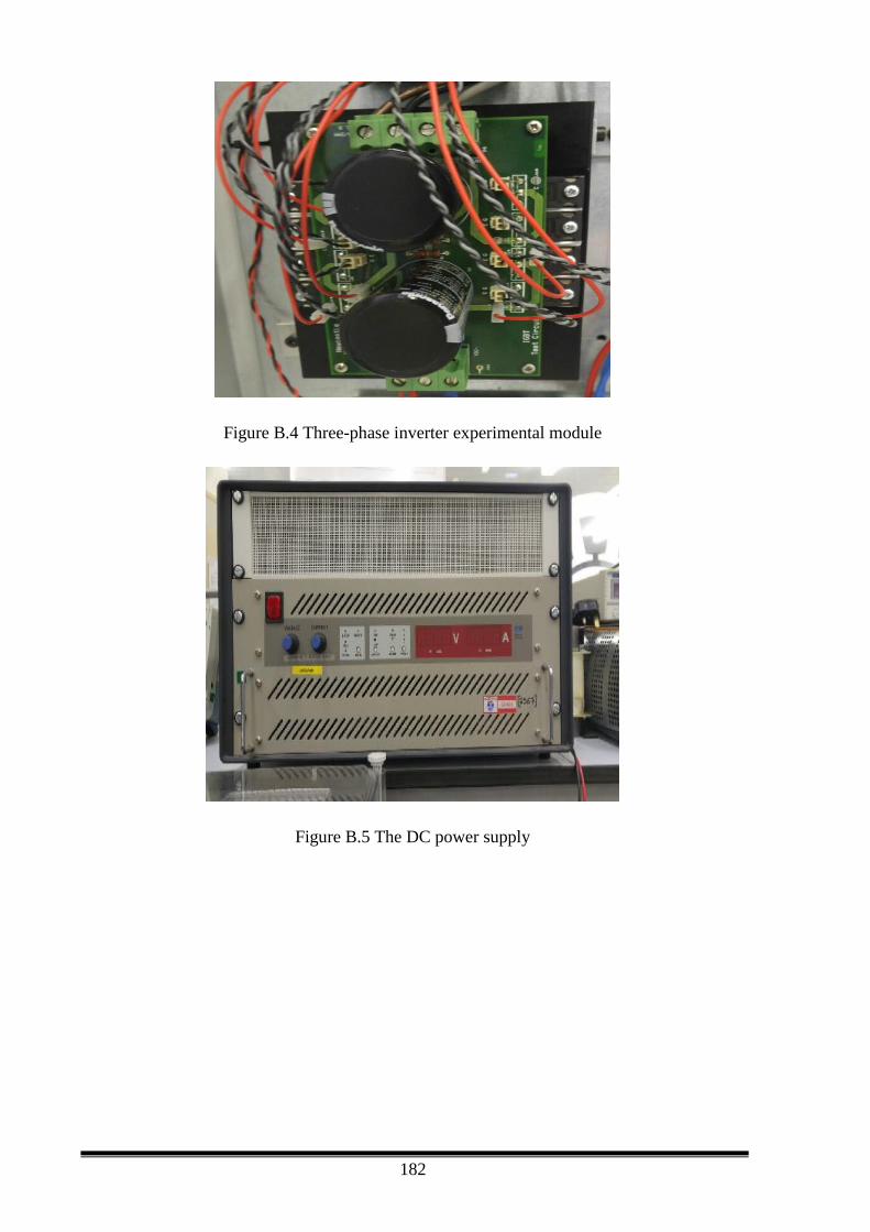
182
Figure B.4 Three-phase inverter experimental module
Figure B.5 The DC power supply
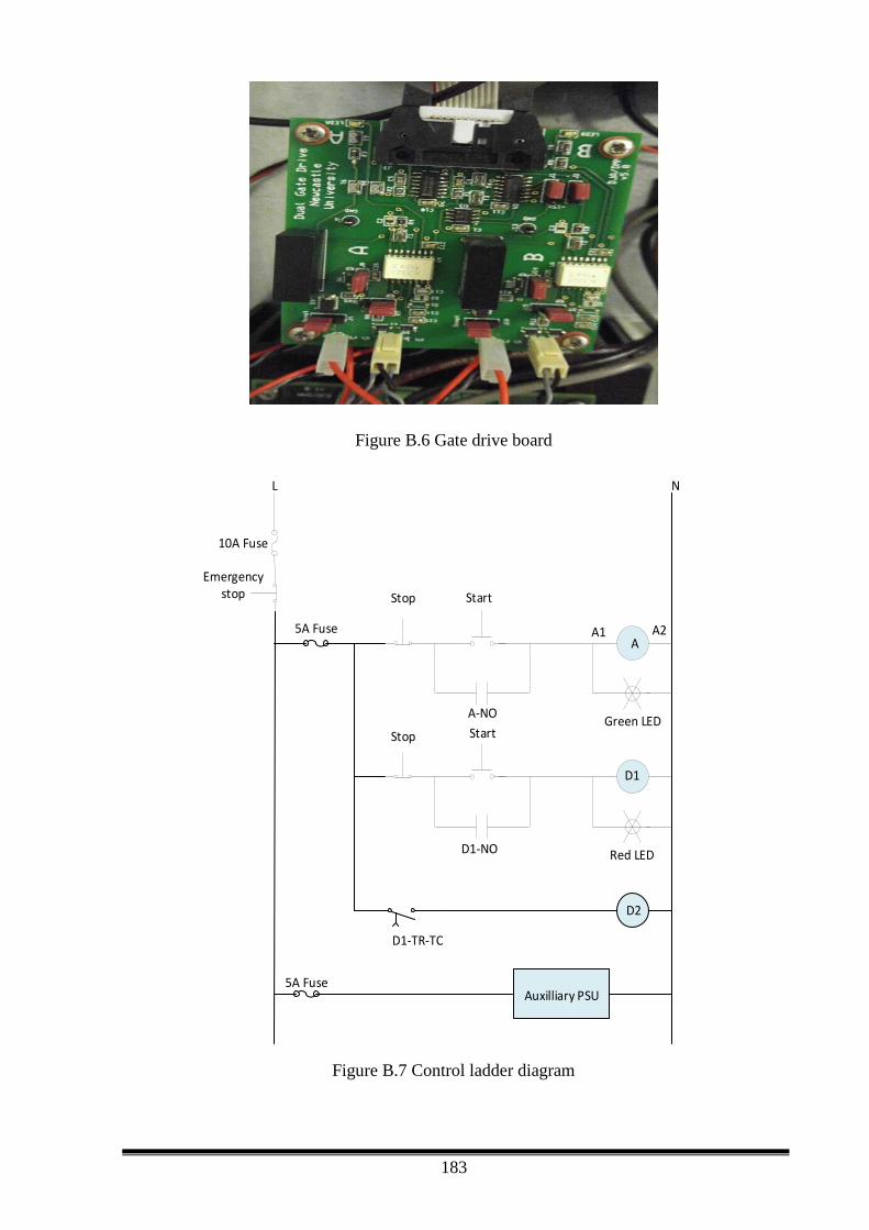
183
Figure B.6 Gate drive board
L N
10A Fuse
Emergencystop Stop Start
A
A-NO
A1 A2
Stop Start
D1
D2
D1-NO
D1-TR-TC
Auxilliary PSU
Green LED
Red LED
5A Fuse
5A Fuse
Figure B.7 Control ladder diagram

184
B.4 Digital Signal Processor
Digital signal processor (DSP) is a software card for TMS320F2833x series of floating-point.
This eZdsp kit includes a 12-bit analogue digital converter (ADC) with 16 input channels to
allow data transfer for communication. This card has 128Kx16 asynchronous SRAM, which is
supported to the Code Composer Studio® Integrated Development.
B.5 Analog-to-Digital Converter
In power electronics, Analog-to-digital converter (ADC) is used to convert analogue signals
such as the voltage signal into digital signal. ADC has employed 16 converting channels built-
in which has 12-bit ADC core that sample-and-hold acquired.
B.6 Current Sensor
The current sensor is very important part of the three-phase grid-connected inverter in order to
measure and control the current with the varying weak grid. Figure B.7 shows the schematics
of the current sensor. It is important for the safety and protection of the power electronics rig
from over current and any fault that occurs. In industry, there are many types of current sensors.
One of these current sensors is CAS15-NP. This type of the current sensor has many features.
It designed to work up to 50 A, and has a very low-temperature coefficient of offset. It has a
galvanic isolation and it has high flexibility with reliability. It can work with different
applications.
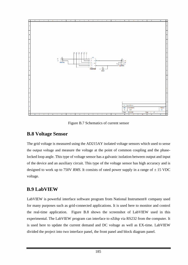
185
Figure B.7 Schematics of current sensor
B.8 Voltage Sensor
The grid voltage is measured using the AD215AY isolated voltage sensors which used to sense
the output voltage and measure the voltage at the point of common coupling and the phase-
locked loop angle. This type of voltage sensor has a galvanic isolation between output and input
of the device and an auxiliary circuit. This type of the voltage sensor has high accuracy and is
designed to work up to 750V RMS. It consists of rated power supply in a range of ± 15 VDC
voltage.
B.9 LabVIEW
LabVIEW is powerful interface software program from National Instrument® company used
for many purposes such as grid-connected applications. It is used here to monitor and control
the real-time application. Figure B.8 shows the screenshot of LabVIEW used in this
experimental. The LabVIEW program can interface to eZdsp via RS232 from the computer. It
is used here to update the current demand and DC voltage as well as EX-time. LabVIEW
divided the project into two interface panel, the front panel and block diagram panel.
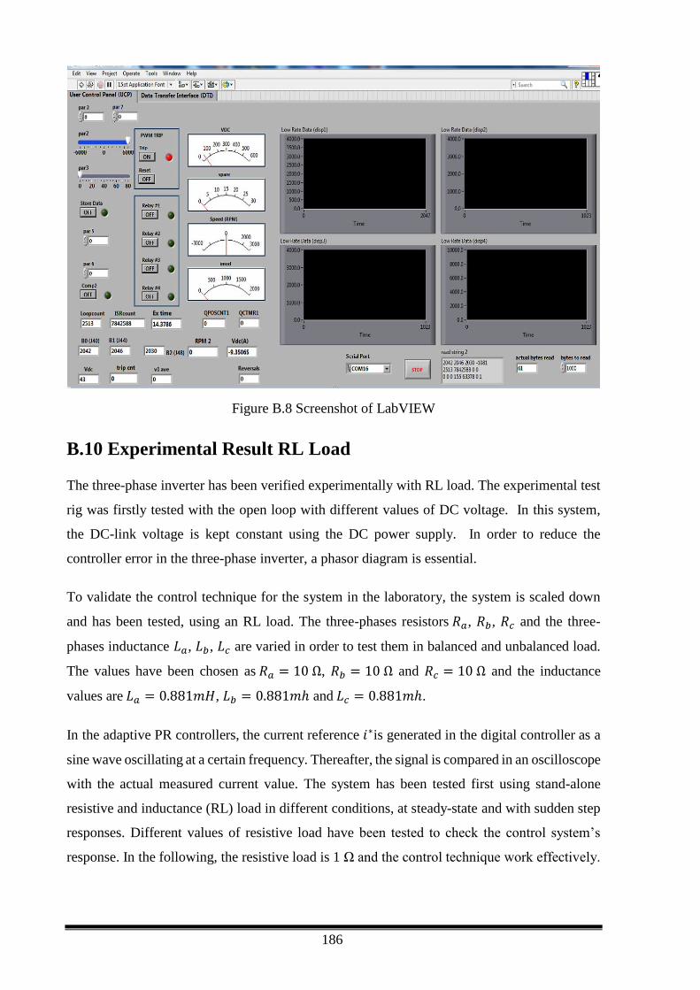
186
Figure B.8 Screenshot of LabVIEW
B.10 Experimental Result RL Load
The three-phase inverter has been verified experimentally with RL load. The experimental test
rig was firstly tested with the open loop with different values of DC voltage. In this system,
the DC-link voltage is kept constant using the DC power supply. In order to reduce the
controller error in the three-phase inverter, a phasor diagram is essential.
To validate the control technique for the system in the laboratory, the system is scaled down
and has been tested, using an RL load. The three-phases resistors 𝑅𝑎, 𝑅𝑏, 𝑅𝑐 and the three-
phases inductance 𝐿𝑎, 𝐿𝑏, 𝐿𝑐 are varied in order to test them in balanced and unbalanced load.
The values have been chosen as 𝑅𝑎 = 10 Ω, 𝑅𝑏 = 10 Ω and 𝑅𝑐 = 10 Ω and the inductance
values are 𝐿𝑎 = 0.881𝑚𝐻, 𝐿𝑏 = 0.881𝑚ℎ and 𝐿𝑐 = 0.881𝑚ℎ.
In the adaptive PR controllers, the current reference 𝑖∗is generated in the digital controller as a
sine wave oscillating at a certain frequency. Thereafter, the signal is compared in an oscilloscope
with the actual measured current value. The system has been tested first using stand-alone
resistive and inductance (RL) load in different conditions, at steady-state and with sudden step
responses. Different values of resistive load have been tested to check the control system’s
response. In the following, the resistive load is 1 Ω and the control technique work effectively.
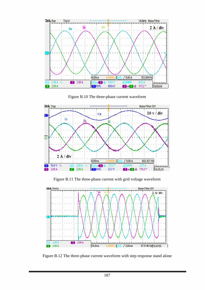
187
Figure B.10 The three-phase current waveform
Figure B.11 The three-phase current with grid voltage waveform
Figure B.12 The three-phase current waveform with step response stand alone
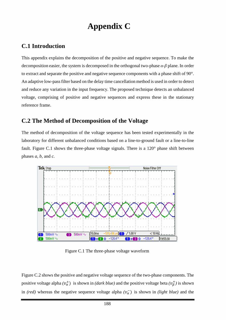
188
Appendix C
C.1 Introduction
This appendix explains the decomposition of the positive and negative sequence. To make the
decomposition easier, the system is decomposed in the orthogonal two-phase α-β plane. In order
to extract and separate the positive and negative sequence components with a phase shift of 90°.
An adaptive low-pass filter based on the delay time cancellation method is used in order to detect
and reduce any variation in the input frequency. The proposed technique detects an unbalanced
voltage, comprising of positive and negative sequences and express these in the stationary
reference frame.
C.2 The Method of Decomposition of the Voltage
The method of decomposition of the voltage sequence has been tested experimentally in the
laboratory for different unbalanced conditions based on a line-to-ground fault or a line-to-line
fault. Figure C.1 shows the three-phase voltage signals. There is a 120° phase shift between
phases a, b, and c.
Figure C.1 The three-phase voltage waveform
Figure C.2 shows the positive and negative voltage sequence of the two-phase components. The
positive voltage alpha (𝑣𝛼+) is shown in (dark blue) and the positive voltage beta (𝑣𝛽
+) is shown
in (red) whereas the negative sequence voltage alpha (𝑣𝛼−) is shown in (light blue) and the
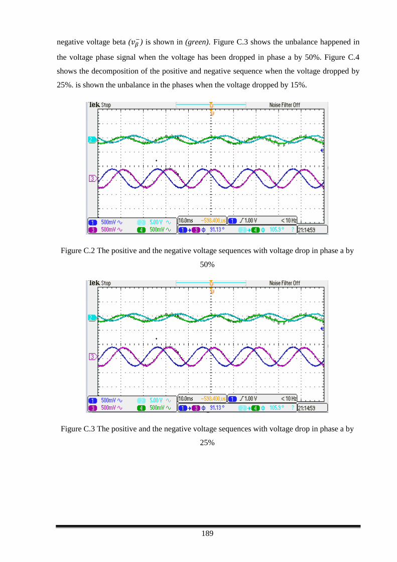
189
negative voltage beta (𝑣𝛽−) is shown in (green). Figure C.3 shows the unbalance happened in
the voltage phase signal when the voltage has been dropped in phase a by 50%. Figure C.4
shows the decomposition of the positive and negative sequence when the voltage dropped by
25%. is shown the unbalance in the phases when the voltage dropped by 15%.
Figure C.2 The positive and the negative voltage sequences with voltage drop in phase a by
50%
Figure C.3 The positive and the negative voltage sequences with voltage drop in phase a by
25%
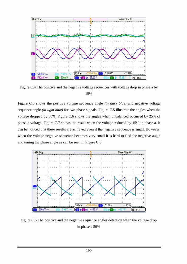
190
Figure C.4 The positive and the negative voltage sequences with voltage drop in phase a by
15%
Figure C.5 shows the positive voltage sequence angle (in dark blue) and negative voltage
sequence angle (in light blue) for two-phase signals. Figure C.5 illustrate the angles when the
voltage dropped by 50%. Figure C.6 shows the angles when unbalanced occurred by 25% of
phase a voltage. Figure C.7 shows the result when the voltage reduced by 15% in phase a. It
can be noticed that these results are achieved even if the negative sequence is small. However,
when the voltage negative sequence becomes very small it is hard to find the negative angle
and tuning the phase angle as can be seen in Figure C.8
Figure C.5 The positive and the negative sequence angles detection when the voltage drop
in phase a 50%
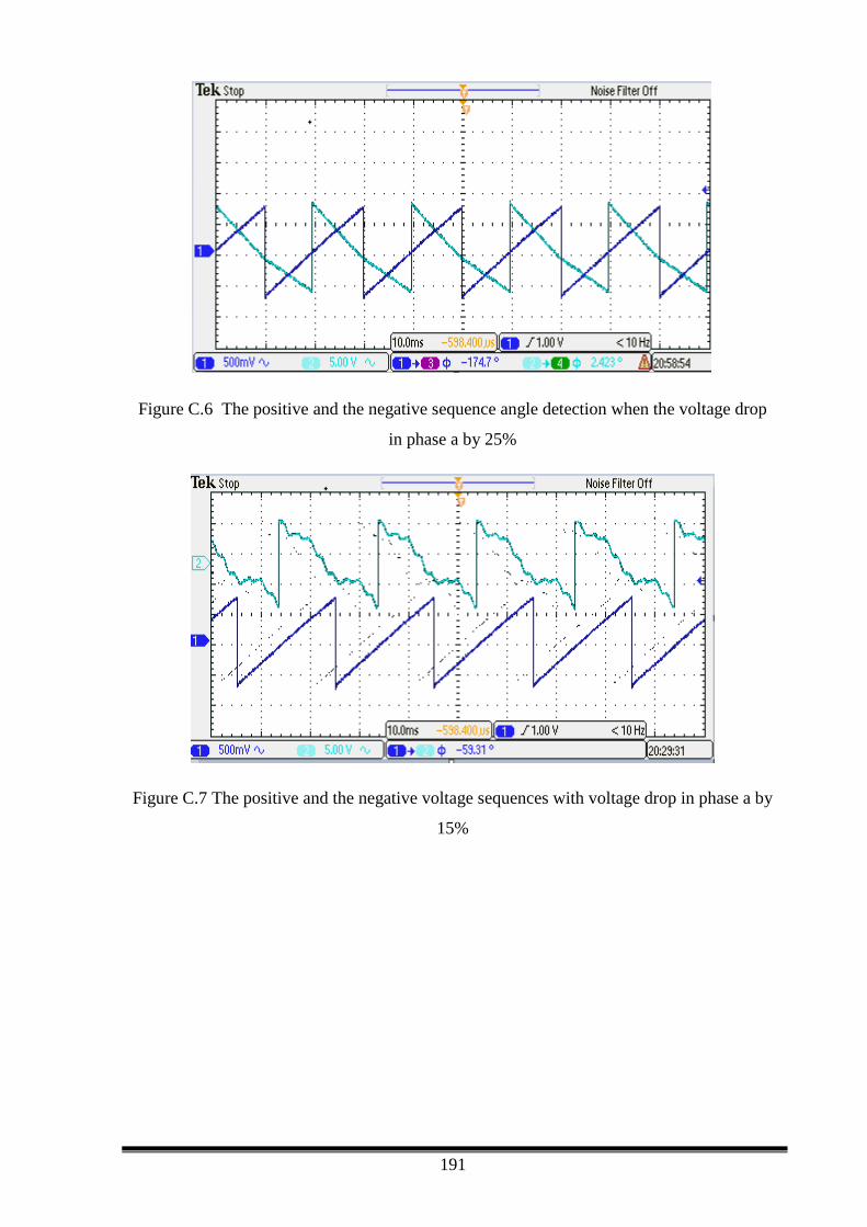
191
Figure C.6 The positive and the negative sequence angle detection when the voltage drop
in phase a by 25%
Figure C.7 The positive and the negative voltage sequences with voltage drop in phase a by
15%
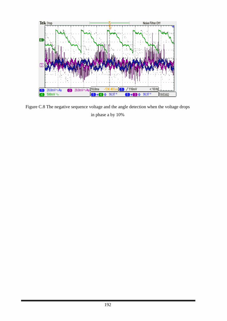
192
Figure C.8 The negative sequence voltage and the angle detection when the voltage drops
in phase a by 10%

193

194
![Proportional-resonant controllers and filters for grid-connected … · 2020. 5. 25. · uninterruptible power supplies (UPS) and in [9] for single-phase photovoltaic (PV) inverters](https://img.pdfslide.net/doc/110x75/60f2bdc4a261982e59389d17/proportional-resonant-controllers-and-ilters-for-grid-connected-2020-5-25.jpg)


![FREQUENCY-BASED ENERGY MANAGEMENT IN ISLANDED MICROGRID · 2018. 3. 28. · proportional-resonant (PR) [7]. Dan Wu1, Fen Tang, Josep M. Guerrero, and Juan C. Vasquez proposed a microgrid,](https://img.pdfslide.net/doc/110x75/604b24bdd7ce3d482f165b7d/frequency-based-energy-management-in-islanded-microgrid-2018-3-28-proportional-resonant.jpg)