TRANSPORTATION MODELING

Modeling Concept

Model

Tools and media to reflect and simple a measured reality.

Types of Model

Physical Model

Map and Chart Model

Statistics and mathematical Models

MODEL?

Physical Model

Map Model (Desire Line)

Map Model

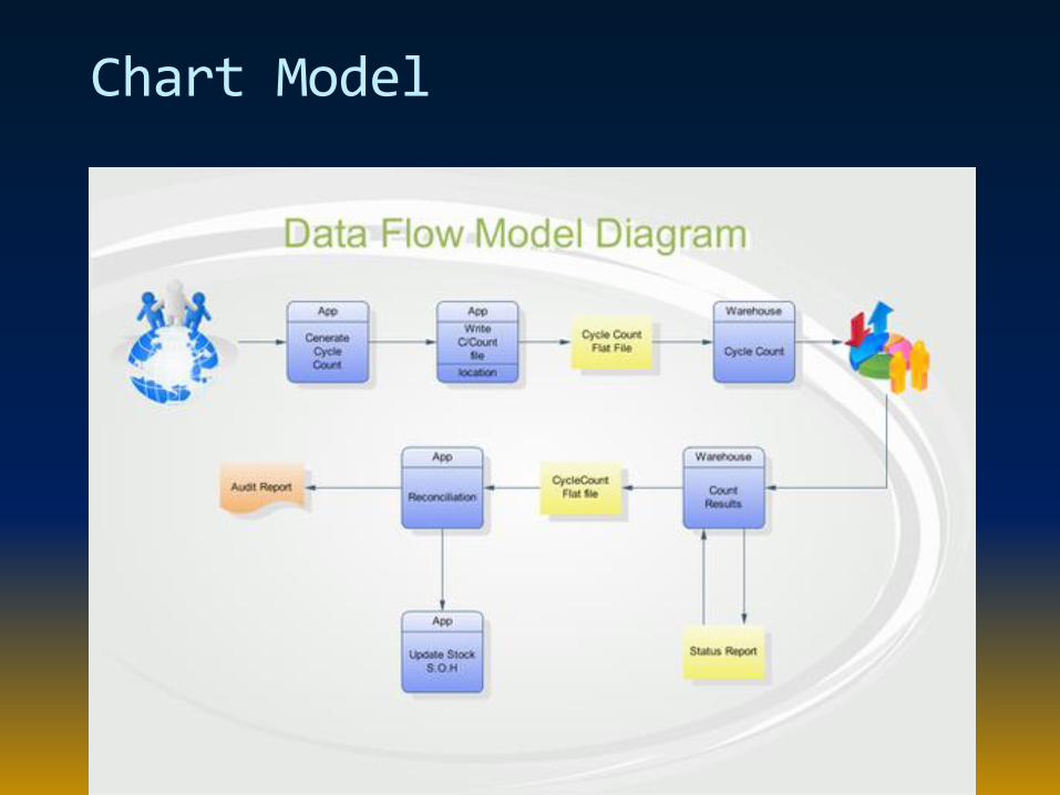
Chart Model

Chart Model

Statistic and Mathematical Models

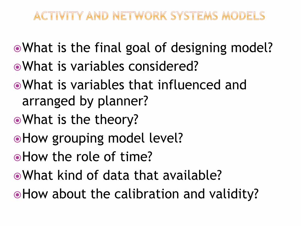
What is the final goal of designing model?

What is variables considered?

What is variables that influenced and

arranged by planner?

What is the theory?

How grouping model level?

How the role of time?

What kind of data that available?

How about the calibration and validity?

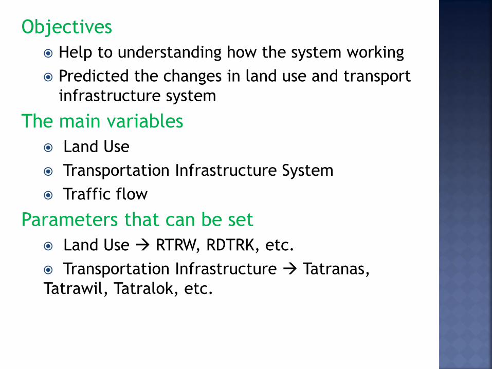
Objectives

Help to understanding how the system working

Predicted the changes in land use and transport

infrastructure system

The main variables

Land Use

Transportation Infrastructure System

Traffic flow

Parameters that can be set

Land Use RTRW, RDTRK, etc.

Transportation Infrastructure Tatranas,

Tatrawil, Tatralok, etc.

Theory/ Concept

Accessibility

Generated and Attracted Trip

Trip Distribution

Mode choice

Route choice

Dynamic Traffic Flow

Grouping Level

Areas?

Combining and Grouping traffic flow?

Time

Static Model

Dynamic Model

Scope Mathematical, statistical, operational research,

programming

Data Quantity

Quality

Calibration and Validation Calibration : process of assessing the parameter

value of a model with various techniques (numerical analysis, linear algebra, optimization, etc.)

Validation : expected models with calibrated parameters before it produce the same output with reality (data) forecasting future

Modification : Reduction or addition of several variables suit for the applications in the area or another condition.

Determination of the study area

Study area divided into several zones,

numbers and areas depend on level of

accuracy expected

The Outside of study area divided into

several external zones to reflect the

other zones

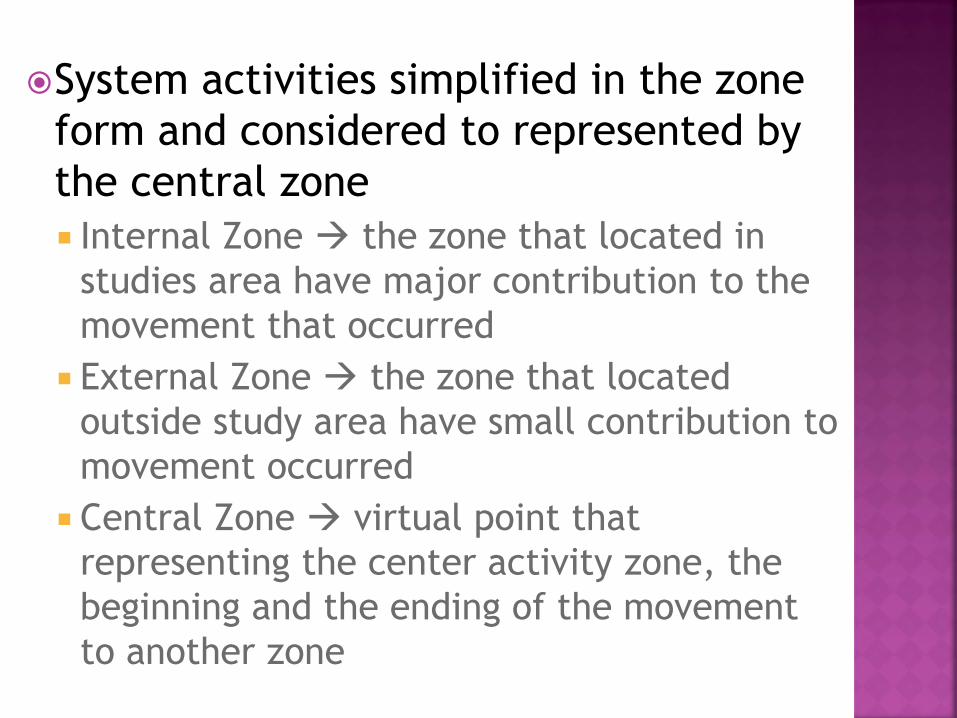
System activities simplified in the zone

form and considered to represented by

the central zone

Internal Zone the zone that located in

studies area have major contribution to the

movement that occurred

External Zone the zone that located

outside study area have small contribution to

movement occurred

Central Zone virtual point that

representing the center activity zone, the

beginning and the ending of the movement

to another zone

Network system that simplified in road

and joint form

Road segment or railway network, etc.

The segment must have information of road

conditions

Node intersection, station, city, etc.

Activity and Network systems was

connected with central zone

Central Zone Link virtual segment that

connected to the central zone (activity

system) by a node (network system)

1 2

3

6

5

4

Border Study

Study area

Internal Zone

Central Zone

Border area

Study area

Road

Node

gateway

1 2

3

6

5

4

Border area

Study area

Zone center link

1 2

3

6

5

4

Combined Cost Concept

Combining three main components of route choice (Distance, cost, time)

Combined cost of private cars

Gcp = yD + uTv + C

Where :

Gcp = Combined cost for PC (Rp)

y = Operating vehicle cost per unit distance

(Rp/km)

C = parking cost, toll, etc.

Combined cost for public transport:

Gcu = fD + u Ta + u Tw + u Tv + d

Where :

Gcu = Combined cost for PT (Rp)

D = Distance (distance unit, e.g : km)

Ta = walking time (time unit, e.g: minutes)

Tw = waiting time PT (time unit, e.g: minutes)

Tv = time in public transportation (time unit, e.g: minutes)

f = cost per distance (Rp/km)

u = time value per unit time (Rp/minutes)

d = surcharge unmeasured

A Simple Model of Land Use / Transport System

Objectives:

Help to understand how the transportation system works

Predict the changes in traffic flows which will result from changes to land use or to the transport system

Variables:

Land Use System : population and employment

Transport system : Distance, Travel time

Traffic System

Notasi:

LA,B = Land Use in Zone A, B

PA = Traffic Generation from zone A

AB = Traffic Attraction to zone B

QAB(1) = Traffic from zone A to zone B using route 1

TQAB(1) = Travel time from zone A to zone B using in

traffic condition is Q

T0 = Travel time in free-flow traffic = 0

C = Road capacity

a = Level of Service index

Traffic Generation

PA = f (LA)

AB = f (LB)

Traffic Distribution

QAB = PA.AB.k

TQAB

Mode and Route Choice

TQAB(1) = TQAB(2)

Activity system : Zone Land Use Population Information

A Residential 35.000 90% working age

B Employment area

12.000

Transport characteristic:

Route Length (km)

To (min.)

Los Index (a)

Capacity (veh/h)

1 17 25 0,4 3.000

2 20 40 1,0 2.000

3 14 20 0,25 4.000

Traffic Distribution

QAB = PA.AB.0,001

TQAB

1. The amount of traffic from zone A to zone B if only route 1 that operated?

2. The amount of traffic from zone A to zone B if only route 2 that operated?

3. The amount of traffic from zone A to zone B if route 1 and 2 operating together?

4. The amount of traffic if adding a new road 3 and route 1,2, and 3 are operated together?

5. The amount of traffic if there are changes in residential population become 40.000 and employment population 20.000?

Solution

‘Demand’ Equation:

QAB = 31.500 x 12.000 x 0,001

TQAB

= 378.000

TQAB

‘Supply’ Equation:

Route 1:

TQAB(1) = 25 x (3.000 – 0.6 QAB(1))

3.000 – QAB(1)

Route 2:

TQAB(2) = 40 x 2.000

2.000 – QAB(2)

Route 3:

TQAB(3) = 20 x (4.000 – 0.75 QAB(3))

4.000 – QAB(3)

Analytical method

If only route 1 that operated:

Then:

TQAB(1) = 378.000

QAB(1)

( 75.000 – 15 QAB(1)) x QAB(1) = (3.000 – QAB(1)) x 378.000

15 QAB(1)2 – 453.000QAB(1) + 1.134.000.000 = 0

QAB(1) = 2.755 veh/h TQAB(1) = 137,2 minutes

QAB(1) = 2.755 QAB(1) = 27.445 (>>C1)

If only route 2 that operated:

TQAB(2) = 378.000

QAB(2)

80.000 x QAB(2) = (2.000 – QAB(2)) x 378.000

458.000QAB(2) + 756.000.000 = 0

QAB(2) = 1.651 veh/h TQAB(2) = 229 minutes

If route 1+2 operating together:

(1)

Equal condition 1 and 2:

TQAB = 378.000 = 378.000

QAB QAB(1) +QAB(2)

Limit 1: QAB = QAB(1) + QAB(2)

Limit 2: TQAB = TQAB(1) = TQAB(2)

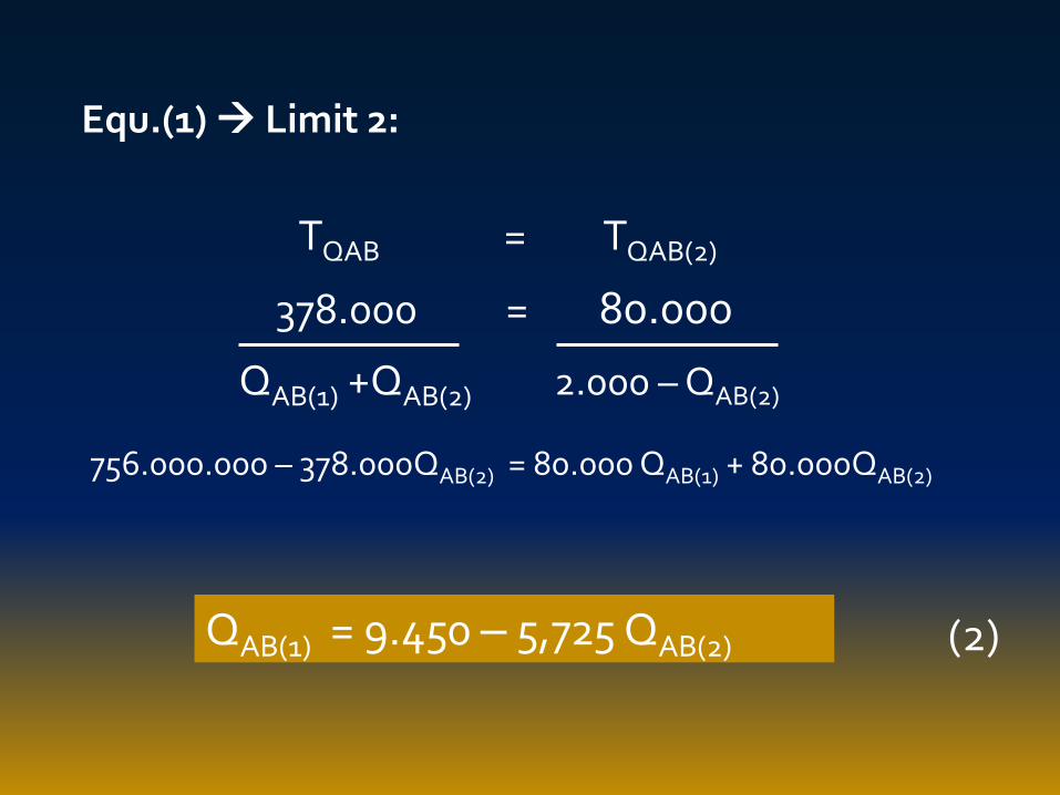
Equ.(1) Limit 2:

TQAB = TQAB(2)

378.000 = 80.000

QAB(1) +QAB(2) 2.000 – QAB(2)

756.000.000 – 378.000QAB(2) = 80.000 QAB(1) + 80.000QAB(2)

QAB(1) = 9.450 – 5,725 QAB(2) (2)

75.000 – 15 QAB(1) = 80.000

3.000 – QAB(1) 2.000 – QAB(2)

150.000.000 – 75.000QAB(2) – 30.000QAB(1) – 15QAB(1)QAB(2) = 240.000.000 – 80.000QAB(1)

50.000QAB(1) – 15QAB(1) QAB(2) – 75.000QAB(2) = 90.000.000

(2)

Limit 2: TQAB(1) = TQAB(2)

Substitution (1) to (2):

50.000 (9.450 – 5,725 QAB(2)) – 15 (9.450 – 5,725 QAB(2)) QAB(2) –

75.000QAB(2) = 90.000.000

Obtainable:

Then :

85,875QAB(2) 2 + 219.500 QAB(2) – 382.500.000 = 0

(3)

QAB(2) = 1.189 veh/h TQAB(2) = 98,675 mins.

QAB(1) = 2.641 veh/h TQAB(1) = 98,675 mins.

QAB = 3.830 veh/h TQAB = 98,675 mins.

QAB(2) = 1.189 QAB(2) = -3.745(-, impossible)

If route 1+2+3 operating together:

TQAB = 378.000 = 378.000

QAB QAB(1) +QAB(2) +QAB(3)

(1)

Limit 1:

Limit 1: QAB = QAB(1) + QAB(2)+ QAB(3)

Limit 2: TQAB = TQAB(1) = TQAB(2) = TQAB(3)

Graphical method

From the equation demand and supply, input value of QAB to obtain value of TQAB, TQAB(1), TQAB(2) or TQAB(3)

Plot the value of QAB and TQAB, to obtain the demand curve

Plot the value of QAB and TQAB(1), TQAB(2) or TQAB(3) to obtain supply curve route 1, 2 and 3

Cutting point between demand and supply curve is a equilibrium point

QAB TQAB

0 ~

500 756.00

1000 378.00

1500 252.00

2000 189.00

2500 151.20

3000 126.00

3500 108.00

4000 94.50

4500 84.00

5000 75.60

5500 68.73

6000 63.00

6500 58.15

7000 54.00

7500 50.40

8000 47.25

8500 44.47

9000 42.00

QAB TQAB(1) TQAB(2) TQAB(3)

0 25.00 40.00 20.00

500 27.00 53.33 20.71

1000 30.00 80.00 21.67

1500 35.00 160.00 23.00

2000 45.00 ~ 25.00

2500 75.00 28.33

3000 ~ 35.00

3500 55.00

4000 ~

4500

5000

5500

6000

6500

7000

7500

8000

8500

9000

Demand Supply

0

50

100

150

200

250

300

350

400

450

5000

500

100

0

150

0

20

00

250

0

300

0

350

0

40

00

450

0

500

0

550

0

60

00

650

0

700

0

750

0

80

00

850

0

90

00

950

0

100

00

T (

Tra

vel t

ime

- m

inu

tes)

Q (Vehicle per hour)

Relationship between QAB and TQAB

Demand

Supply 1

Supply 2

Supply 3

0

50

100

150

200

250

300

350

400

450

500

0

500

100

0

150

0

20

00

250

0

300

0

350

0

40

00

450

0

500

0

550

0

60

00

650

0

700

0

750

0

80

00

850

0

90

00

950

0

100

00

T (

Tra

vel t

ime

, m

inu

tes)

Q (Vehicle per hour)

Relationship between QAB and TQAB

Demand

Supply 1

Supply 2

Supply 3

Supply 1+2

Supply 1+2+3

0

50

100

150

200

250

300

350

400

450

500

0

500

100

0

150

0

20

00

250

0

300

0

350

0

40

00

450

0

500

0

550

0

60

00

650

0

700

0

750

0

80

00

850

0

90

00

950

0

100

00

T (

Tra

vel t

ime

, m

inu

tes)

Q (vehicle per hour)

Relationship between QAB and TQAB

Demand

Supply 1

Supply 2

Supply 3

Supply 1+2

Supply 1+2+3

Demand Baru

Transportation Characteristic:

Another data same with example before

Route Length (km)

To (minutes)

LoS index (a)

Capacity (veh/h)

1 15 20 0,5 3.000

2 25 45 0,9 2.000

Assignment

Complete with analytical method:

1. The amount of traffic from zone A to zone B if only route 1 that operated?

2. The amount of traffic from zone A to zone B if only route 2 that operated?

3. The amount of traffic from zone A to zone B if route 1 and 2 operating together?