Embed Size (px)
Citation preview
Propositional Proof Complexity
Instructor: Alexander Razborov, University of [email protected]
Course Homepage:http://people.cs.uchicago.edu/~razborov/teaching/winter09.html
Winter, 2009 and Winter, 2014
Contents
1 Global Picture 2
2 Size-Width Tradeoff for Resolution 32.1 Resolution Proof System . . . . . . . . . . . . . . . . . . . . . 32.2 Width: Another Complexity Measure . . . . . . . . . . . . . 42.3 Restrictions . . . . . . . . . . . . . . . . . . . . . . . . . . . . 52.4 Edge Expansion Gives a Width Lower Bound . . . . . . . . . 6
3 Bounded Arithmetic: Theory of Feasible Proofs 83.1 Axioms for Bounded Arithmetic . . . . . . . . . . . . . . . . 83.2 The Main Theorem of Bounded Arithmetic . . . . . . . . . . 10
3.2.1 Bootstrapping by Introducing New Symbols . . . . . . 113.2.2 Finite Sequences . . . . . . . . . . . . . . . . . . . . . 123.2.3 Hentzen Calculus . . . . . . . . . . . . . . . . . . . . . 13
3.3 RSUV isomorphism . . . . . . . . . . . . . . . . . . . . . . . . 153.4 The bounded arithmetic hierarchy . . . . . . . . . . . . . . . 163.5 Does this hierarchy collapse? . . . . . . . . . . . . . . . . . . 163.6 More witnessing theorems . . . . . . . . . . . . . . . . . . . . 183.7 Transition to propositional logic . . . . . . . . . . . . . . . . . 20
4 Interpolation and Automatizability 204.1 Feasible Interpolation . . . . . . . . . . . . . . . . . . . . . . 204.2 Automatizability . . . . . . . . . . . . . . . . . . . . . . . . . 204.3 Resolution is Probably not Automatizable . . . . . . . . . . . 25
4.3.1 Constructing the contradiction . . . . . . . . . . . . . 28
1
4.3.2 The Upper Bound on sR . . . . . . . . . . . . . . . . . 314.3.3 The Lower Bound on sR . . . . . . . . . . . . . . . . . 324.3.4 Combinatorial Voodoo . . . . . . . . . . . . . . . . . . 354.3.5 The Upper Bound when k(C) is too large . . . . . . . 36
5 Applications to Learning 365.1 Decision Trees . . . . . . . . . . . . . . . . . . . . . . . . . . . 37
6 Concrete Lower Bounds 396.1 Random 3-CNFs . . . . . . . . . . . . . . . . . . . . . . . . . 396.2 The Pigeon-Hole Principle . . . . . . . . . . . . . . . . . . . . 39
6.2.1 Matching Restrictions . . . . . . . . . . . . . . . . . . 406.2.2 Matching Decision Trees . . . . . . . . . . . . . . . . . 416.2.3 Putting it all together . . . . . . . . . . . . . . . . . . 41
7 Algebraic and Geometric proof systems 437.1 Algebraic proof systems . . . . . . . . . . . . . . . . . . . . . 43
7.1.1 Nullenstellensatz proof systems . . . . . . . . . . . . . 437.1.2 Polynomial Calculus . . . . . . . . . . . . . . . . . . . 447.1.3 Algebraic calculus and logic . . . . . . . . . . . . . . . 48
7.2 Geometric proof systems . . . . . . . . . . . . . . . . . . . . . 487.2.1 Cutting planes proof system . . . . . . . . . . . . . . . 49
A Added in 2014 51A.1 Proofs of Resolution Lower Bounds based on Restrictions . . 51A.2 Feasible Interpolation for the Lovasz-Schrijver Proof System . 53A.3 Elements of Space Complexity . . . . . . . . . . . . . . . . . 57
Lecture 1Scribe: Raghav Kulkarni, University of Chicago.
Date: January 6, 2009
1 Global Picture
Question: Intuitively, what makes a proof easy or hard ?a) Length of the proof (e.g., 5 pages vs 10 pages)b) Logical Complexity (e.g., number of quantifiers used)c) Conceptual Complexity (e.g., complexity of the mathematical conceptsused).
2
Types of Proof:1. Proof that uses Quantifiers (e.g., first-order theories)2. Quantifier-free proof (e.g., propositional proof).
In the first part of this course we will briefly study the proofs of type 1but the majority of this course is intended to study the proofs of type 2. Wewill present one particular result in the course which will bridge the part 1with part 2. (This result is roughly of the flavor that “the circuits and theTuring machines are exactly the same in some precise sense.”)
Outreach:a) Lovasz-Schrijver rank : This notion of rank is associated with a positivesemidefinite relaxation of integer linear programs. One consecutively shrinksthe polytope by applying some rules. The rank is roughly the number ofsuch shrinks.b) Applications in Learning.
We begin with a “movie trailer” of the second part.
2 Size-Width Tradeoff for Resolution
Let x1, . . . , xn be propositional variables, i.e., xi ∈ 0, 1.A literal is either xi or ¬xi (sometimes we write ¬x as x).
Let ε ∈ 0, 1. xεi = xi if ε = 1 otherwise ¬xi.A clause C is a disjunction of literals: xε1i1 ∨ . . . ∨ x
εwiw.
The empty clause is denoted by 0.A conjunctive normal form (CNF) formula τ is a conjunction of clauses:C1∧. . .∧Cm. A CNF-formula is unsatisfiable if no assignment of its variablesevaluates to 1 (1 = True). For example, the empty clause 0 is unsatisfiable.An unsatisfiable formula is also called a contradition.
2.1 Resolution Proof System
Question: How does one prove that a CNF-formula τ is unsatisfiable?We prove that τ is unsatisfiable by deducing the empty clause 0 from itsclauses by a series of rules of the following two types:
Resolution Rule:C ∨ x D ∨ x
C ∨DWeakening:
C
C ∨D.
3
Note that one can arrange the intermediate formulae either in a directedacyclic graph (DAG) or unfold the DAG to form a tree-like proof system.
(Soundness Theorem) If one can deduce 0 from τ by applying the aboverules, then τ is unsatisfiable.(Completeness Theorem) If τ is unsatisfiable then τ ` 0, i.e., one candeduce 0 from τ. (Homework 1.)
Let P be a resolution(refutation) of τ. We denote by |P | the total num-ber of clauses in P.SR(τ) = min|P | : P is a refutation of τ.Question: Are there short CNF-formulae which require large refutation ?Historical background:Tseitsin [68] - answered the question for regular resolutions.Haken [85] - constructed τ such that all of its refutations are exponential.Chvatal-Szemeredi [88] - random CNF is almost surely unsatisfiable and hasonly exponentially long refutation proofs.The above results are extremely nice and important but somewhat ad hoc.
2.2 Width: Another Complexity Measure
The width of a clause: w(xε11 ∨ . . . ∨ xεwiw
) = w.w(τ) = maxw(C) : C ∈ τ.w(P ) = maxw(C) : C ∈ P.wR(τ) = minw(P ) : P − refutation of τ.Question: What is the relation between w(τ) and wR(τ) ?If we use all clauses in τ then wR(τ) ≥ w(τ) but it is not true in general.One might not use all clauses of τ for its refutation, one might be able todeduce 0 from a subset of its clauses.Question: What is the relation between SR(τ) and wR(τ) ?
It is easy to see that SR(τ) ≤ (2n)wR(τ).Question: Does the above inequality hold in the other direction ?Unfortunately, wR(τ) ≤ lognSR(τ) is not true exactly, but the followingtheorem is known.
Theorem 1 (Ben-Sasson Wigderson 99). For any n-variable contradictionτ, wR(τ) = O(
√n logSR(τ)).
If τ is a contradiction and wR(τ) = Ω(n) then SR(τ) = exp(Ω(n)).
4
Remark: Bonet, Galesi [99] - the bound in Theorem 1 is almost tight.In particular, for every n, there is an n-variable contradiction τn such thatSR(τn) = nO(1) but wR(τn) = Ω(
√n).
2.3 Restrictions
For a clause C, its restriction to x = ε is defined as follows:C|x=ε = C if x /∈ C; 1 if C = D ∨ xε; D if D = D ∨ x1−ε.If τ = C1 ∧ . . . ∧ Cm, then τ |x=ε = C1|x=ε ∧ . . . ∧ Cm|x=ε.
Exercise: If τ is a contradiction then so is τ |x=ε. Moreover, the restrictionof a refutation (of τ) is again a refutation (of τ |x=ε).
Lemma 2.1 (Restriction is simpler to refute). wR(τ |x=ε) ≤ wR(τ).
It is interesting that one can prove the following lemma in the other direc-tion.
Lemma 2.2. wR(τ) ≤ maxwR(τ |x=0), wR(τ |x=1)+ 1.
Exercise: Prove Lemma 2.1 and Lemma 2.2.
Next time, we will show that a slightly stronger version of the above lemmaholds. In particular, we will prove that:if wR(τ |x=ε) ≤ w − 1 and wR(τ |x=1−ε) ≤ w, then wR(τ) ≤ w.We will see in the next lecture that this crucial inequality leads to the proofof Theorem 1.
Lecture 2Scribe: Raghav Kulkarni, University of Chicago.
Date: January 8, 2009
Lemma 2.3. If wR(τ |x=ε) ≤ w− 1 and wR(τ |x=1−ε) ≤ w, then wR(τ) ≤ w.
Proof: The idea is to do the refutations sequentially. First deduce x1−ε
from τ using clauses of width at most w. (Follow closely the deduction from
5
τ |x=ε to 0, which uses clauses of length at most w − 1. Add x1−ε to everyclause in such a deduction.) Now, from x1−ε and τ, deduce τ |x=1−ε by usingthe resolution rule. This step does not introduce any clause of width morethan w. Finally, deduce 0 from τ |x=1−ε using clauses of width at most w.
Fat Clause: C is called fat if w(C) > d. (d is a parameter to be specifiedlater)
Lemma 2.4. If P is a refutation of τ that contains less than ab fat clausesthen wR(τ) ≤ d+ b where a = (1− d
2n)−1.
Proof: We do induction on b and n.Base case: b = 0 ⇒ no fat clauses ⇒ wR(τ) ≤ d.Let C1, C2, . . . , Ck be all the fat clauses in P. Note that, out of the 2n lit-erals, there exists xε such that xε is contained in d
2n × k clauses. Withoutloss of generality, let xε = x be such a literal. By induction on b we havewR(τ |x=1) ≤ d + b − 1 and by induction on n we have wR(τ |x=0) = d + b.From Lemma 2.3, R(τ) ≤ d+ b.
Now we begin the proof of Theorem 1. Proof: Let ab = SR(τ)
⇒ b = logSR(τ)log a = O(nd logSR(τ))
⇒ wR(τ) = O(d+ nd logSR(τ)).
Choose d =√n logSR(τ) to minimize the RHS.
Corollary: wR(τ) = Ω(n)⇒ SR(τ) = exp(Ω(n)).
Applications of Theorem 1:Usually it is easier to prove a lower bound on width than on size. FromTheorem 1, one can deduce a lower bound on the size from a lower boundon the width. The above theorem is used in proving lower bounds for thesize of the refutations of the following:a) Pigeon Hole Principleb) Random 3-CNFc) Tseitin tautologies (introduced in 1968).
For an alternate way of converting width lower bounds into size lowerbounds see Appendix A.1.
2.4 Edge Expansion Gives a Width Lower Bound
Let G be a fixed graph on n vertices. Let xe | e ∈ E(G) be the set ofvariables. Let f : V (G)→ 0, 1 be such that ⊕v∈V (G)f(v) ≡ 1 mod 2. Let
6
τ(G, f) ≡ (∀v ∈ V (G))(⊕e3vxe = f(v)). Suppose we want to refute τ(G, f).Let d = maxdegG(v) | v ∈ V (G). It is easy to see that τ(G, f) is a d-CNFwith at most dn
2 variables and at most n× 2d−1 clauses.
Edge Expansion: e(G) = minn3≤|V |≤ 2n
3e(V, V (G)\V ).
Theorem 2 (Ben-Sasson and Wigderson 99). For any connectedG, wR(τ(G, f)) ≥e(G).
Axioms:⊕v∈V (G)f(v) ≡ 1 mod 2.Av : ⊕e∈vxe ≡ f(v) mod 2.
A Measure on Clauses:For a clause C, µ(C) = min|V | : Av | v ∈ V |= C.
Exercise: If C ∈ τ(G, f) then µ(C) ≤ 1.
Exercise: If G is connected then µ(0) = n.
Exercise: (µ(C ∨ x) ≤ a&µ(D ∨ x) ≤ b)⇒ µ(C ∨D) ≤ a+ b.
Exercise: (Intermediate Clause:) (∃C)(n3 ≤ µ(C) ≤ 2n3 ).
Choose any intermediate C. Let V ′ be a minimal set such that Av | v ∈V ′ |= C. Since C is inetrmediate, we have: n
3 ≤ |V′| ≤ 2n
3 . Let e′ = (v′, v) ∈(V ′, V \V ′).Claim: xe appears in C.Proof of Claim: By the minimality of V ′, there exists an assignment Xe | e ∈E(G) which satisfies all the axioms in V ′ exceptAv′ and falsifies C. Supposefor the sake of contradiction that xe′ /∈ C. Note that flipping Xe′ satisfies allthe axioms of V ′ and thus satisfies C. This is a contradiction because thenew assignment still agrees with the old assignment for all variables of C,whereas the old assignment does not satisfy C. Thus, w(C) ≥ e(G), which completes the proof of Theorem 2.
We note that there exist explicit connected graphs G with d = 3 ande(G) ≥ Ω(n). For any such graph, τ(G, f) is exponentially hard to refute inResolution.
7
3 Bounded Arithmetic: Theory of Feasible Proofs
In the next two lectures, we will do the witnessing theorems connecting thefollowing two:a) Logical Complexityb) Conceptual ComplexityFor the purpose of this course, Conceptual Complexity ≡ ComputationalComplexity, i.e., intuitively, the concepts that are easy to compute are sim-ple. Moreover, most often easy to compute means poly-time computable.
Example: (∀x)(1 < x < p ⇒ x - p) ⇒ (∀y)(1 < y < p ⇒ yp−1 ≡ 1 mod p).In the above statement, all the concepts are poly-time computable. For ex-ample, yp−1 can be computed in poly-time by iterated squaring. Thus theabove statement is feasible.On the other hand, the standard proof of already ordy(p) = p − 1 is strik-ingly not feasible. We will see later on that, unless FACTORING is easy,Fermat’s Little Theorem does not possess any feasible proof in the strictsense we are defining.
First Order Theory: A first order theory contains the following:¬,∧,∨,⇒, (∀x), (∃x) and arithmetic over integers.Language: The language of bounded arithmetic consists of the following:S, 0,+, . , |x|, bx/2c,#,≤, where S is the successor function, i.e., S(x) =x+ 1, |x| = “bit-size of x” and #(x, y) = 2|x|·|y|.
Lecture 3Scribe: Joshua A. Grochow, University of Chicago.
Date: January 13, 2009
In these two lectures we continue with bounded arithmetic. We start bynoting that without the # operation, if t is any term, then t(x1, . . . , xn) <(x1 + · · · + xn)O(1), corresponding to linear time. So in order to capturepolynomial time, we need some way to increase bit-sizes faster, which isexactly what # allows us to do. Note that |x#y| = |x||y|; with #, we get|t(x1, . . . , xn)| ≤ (|x1| + · · · + |xn|)O(1), corresponding to polynomial time,as desired.
3.1 Axioms for Bounded Arithmetic
All bounded arithmetics include the axioms BASIC2: these are 32 axiomsthat describe the properties of the logical symbols S, 0, +, ·, |x|, bx/2c, #,
8
and ≤. Note that these axioms are all quantifier-free (which semanticallyimplies they are implicitly universally quantified, but we don’t want to countsuch implicit quantifiers when we talk about quantifier alternations). Ratherthan list out all the axioms, we ran a PCP protocol with the followingoutputs:
Axiom 17 is |x| = |y| ⇒ x#z = y#z
Axiom 2 is x 6= Sx
Axiom 32 is x = by/2c ⇒ (2 · x = y ∨ S(2 · x) = y).
Throughout, we’ll make use of some standard abbreviations for quanti-fiers, namely, the bounded quantifiers:
(∀x ≤ t)A(x) = (∀x)(x ≤ t⇒ A(x))(∃x ≤ t)A(x) = (∃x)(x ≤ t ∧A(x))
“bounded quantifiers”
and the sharply bounded quantifiers:
(∀x ≤ |t|)A(x) = (∀x)(x ≤ |t| ⇒ A(x))(∃x ≤ |t|)A(x) = (∃x)(x ≤ |t| ∧A(x))
“sharply bounded quantifiers”
Bounded arithmetics also have induction axioms, which are of the form
IND: [A(0) ∧ (∀x)(A(x)⇒ A(Sx))]⇒ (∀x)A(x)
In fact, this an axiom scheme, as there is one axiom for each formula A.Which types of formulae we allow for A determines the strength of theinduction axiom scheme we use.
The class Σbi consists of those formulae that start with an existential
quantifier, and have i quantifier alternations, where we ignore sharply boundedquantifiers. Πb
i is defined similarly, except that the formulae in Πbi begin
with a universal quantifier. Σbk − IND is the induction axiom scheme for all
formula A ∈ Σbk.
The bounded arithmetic T k2 consists of the basic axioms plus Σbk-IND.
This type of induction is not polynomial however. In order to prove A(n),we have to prove A(0), A(1), . . . , A(n− 1) first, which gives proofs of lengthO(n), but that is exponential in the bit-length of n. To remedy this, weintroduce a polynomial induction scheme, which allows induction based onthe bit representation, as follows:
PIND: [A(0) ∧ (A(bx/2c)⇒ A(x))]⇒ (∀x)A(x)
The bounded arithmetic we will be interested in is Sk2 , which consists of thebasic axioms plus Σb
k-PIND.
9
3.2 The Main Theorem of Bounded Arithmetic
The main theorem of bounded arithmetic essentially says that S12 captures
polynomial-time computations:
Theorem 3.
(a) If f(x1, . . . , xk) can be computed in polynomial time, then there existsa Σb
1 formulaA(x1, . . . , xk, y) such that N |= A(n1, . . . , nk, f(n1, . . . , nk))for all n1, . . . , nk ∈ N and S1
2 ` ∀x1, . . . , xk∃!yA(x1, . . . , xk, y). Thatis, S1
2 proves that A is total and single-valued.
(b) IfA(x1, . . . , xk, y) is a Σb1 formula and S1
2 ` ∀x1, . . . , xk∃yA(x1, . . . , xk, y),then there is a polynomial-time computable function f such that |=A(n1, . . . , nk, f(n1, . . . , nk)), and furthermore, S1
2 ` A(n1, . . . , nk, f(n1, . . . , nk)).
Theorems of this sort are called “witnessing theorems.” Note that in(b), we only require that S1
2 prove for each x1, . . . , xk, that there is some ysatisfying A, not necessarily a unique one.
Recall Fermat’s Little Theorem, which we can write as the Σb1 formula:
xn−1 6≡ 1 (mod n)⇒ (∃y ≤ n)(y|n). As a corollary to the above witnessingtheorem, we have:
Corollary 4. If integer factoring is hard (not in polynomial time), then S12
does not prove Fermat’s Little Theorem.
Outline of proof of main theorem. To prove (a), use the definition of P basedon limited iteration (due to Cobham, 1965). Consider the following class offunctions f : Nr → N:
• The constant function 0
• The successor function x 7→ Sx
• Bit-shift x 7→ bx/2c
• Multiplication by 2, x 7→ 2x
• Conditional Choice(x, y, z) = y if x > 0 and z if x = 0
• The characteristic function of ≤, χ≤(x, y)
10
Cobham showed that the closure of these functions under compositionand limited iteration (or recursion) is exactly equal to the class of polynomial-time functions. Before defining limited iteration, we define (unlimited) it-eration: given g : Nr → N and h : Nr+2 → N, we can define τ : Nr+1 → Nby
τ(x, 0) = g(x) and τ(x, n+ 1) = h(x, n, τ(x, n)).
Using limited iteration, such τ can be constructed iff there are polynomialsp and q such that (∀n ≤ p(|x|))(|τ(x, n)| ≤ q(|x|). This forbids construc-tions like τ(0) = 2 and τ(n + 1) = τ(n)2, whose lengths blow up super-polynomially.
Using Cobham’s recursive definition, we can prove (a) first for the func-tions listed above, and then show that if (a) holds for some functions, thenit also holds for their closure under composition and limited iteration.
(Historical aside: Cobham’s definition gave rise to so-called “machine-independent complexity theory” and really got logicians interested in com-plexity.)
We will finish the proof of (a) and outline the proof of (b) next lecture.
Lecture 4Scribe: Joshua A. Grochow, University of Chicago.
Date: January 15, 2009
This lecture will be devoted to finishing the proof of the main witnessingtheorem of bounded arithmetic (that S1
2 exactly captures polynomial-timecomputation). Before continuing, we need a few technical constructions.
3.2.1 Bootstrapping by Introducing New Symbols
Adding new symbols to our language by bootstrapping is essentially onlya matter of convenience, but it makes the proofs much more intelligible.If a theory T proves (∀x)(∃!y)A(x, y), then we can add a new functionsymbol fA(x) and axioms (∀x)A(x, fA(x)) without altering what can beproved in the theory. That is, if a formula B does not contain fA andT + (∀x)A(x, fA(x)) ` B, then T ` B.
When we add a new symbol, we have to be careful how we use induction.In particular, Σb
1-PIND only allows polynomial induction for formulae in theoriginal language, and not formulae with the new symbols. The followinglemma takes care of this technicality, as well as most other technicalities wemight worry about when introducing new symbols in this way:
11
Lemma 3.1. Let A ∈ Σb1 be such that S1
2 ` (∀x)(∃!y)A(x, y), and let T =S1
2 + (∀x)A(x, fA(x)). Then for every B ∈ Σb1(fA), there is a B∗ ∈ Σb
1 suchthat T ` (B ≡ B∗).
Note: we can actually drop the uniqueness from the above statement,but the lemma as stated is all we’ll need.
Hint of proof. We’ll see later that S12 ` (∀x)(∃!y)A(x, y) actually lets us put
a bound on y, that is S12 ` (∀x)(∃!y ≤ t)A(x, y).
The idea is to remove each occurrence of f in B one at a time. SupposeB looks like blah1f(t1, . . . , tr)blah2. Then an equivalent formula is
∃z ≤ t(t1, . . . , tr)[A(t1, . . . , tr, z) ∧ (blah1 z blah2)]
We’ve reduced the number of occurences of f by one, and we haven’t in-creased the complexity since we only added an existential quantifier. (Notethat, since Σb
1 formulae start with an existential quantifier, adding anotherone does not change the complexity of the formula.) Wash, rinse, repeat.
For example, suppose we wish to add the “monus” symbol:
x .− y =
x− y If x ≥ y0 otherwise
Then A(x, y, z) ≡ (y + z = x) ∨ (x ≤ y ∧ z = 0) is a Σb0 ⊆ Σb
1 formula.Existence and uniqueness can be expressed as [A(x, y, z)∧A(x, y, z′)]⇒ z =z′ and (∃z)A(x, y, z), respectively. Both of these follow from the basic axiomsof bounded arithmetic. However, it is hard to show bounded uniqueness inthe form (∃z ≤ x)A(x, y, z); it is easy to prove in T 1
2 , but proving this inS1
2 seems nearly as hard as proving the whole witnessing theorem. This isactual a more general phenomena: the more powerful the theory, the easierit is to bootstrap. When people want to make this harder (to see if it canstill be done), they consider theories such as I∆0, which is S2 =
⋃k S
k2 but
without #.
3.2.2 Finite Sequences
Now we discuss the encoding of finite sequences in bounded arithmetic, e.g.〈x1, . . . , xn〉 where n ≤ |t| for some term t. For this we introduce (aftera fair amount of bootstrapping in the style of the previous section) threefunctions to our language:
12
• UniqSeq(w): a predicate indicating that w is a valid code of a sequence;
• β(i, w): projection function, β(i, 〈x1, . . . , xn〉) = xi; and
• Len(w): the length of w (that is, n).
To complete the proof that all of Cobham’s hierarchy (and hence all ofP) is captured by S1
2 , we essentially need to show two basic facts about finitesequences. First, that they are determined by their projections, namely:
(UniqSeq(A) ∧UniqSeq(B) ∧ Len(A) = Len(B) ∧ (∀i ≤ Len(A))(β(i, A) = β(i, B)))⇒ A = B
and second, we need to show Σb1-replacement (which is essentially the bounded
version of Axiom of Choice). Namely, we’d like to show that for anyA(x, y) ∈ Σb
1, S12 proves
(∀x ≤ |t|)(∃y ≤ s)(A(x, y))⇒ (∃w ≤ SeqBd(s, t))(∀x ≤ |t|)(A(x, β(x,w))∧β(x,w) ≤ s)
where SeqBd is the (bound on) largest w representing a sequence of length≤ |t| and whose elements are all at most s.
With these powerful tools at our disposal, the proof of part a) becomeseasy.
3.2.3 Hentzen Calculus
To prove part (b) of the main witnessing theorem, we will use cut eliminationand Hentzen natural proof systems. In the Hentzen calculus, an implicationsuch as (A1 ∧ · · · ∧Ak)⇒ (B1 ∨ · · · ∨B`) is called a sequent, and we use thenotation A1, . . . , Ak −→ B1, . . . , B`.
The Hentzen calculus has one axiom scheme, A −→ A, and several rulesof logical inference. Here are several examples of such rules:
Γ −→ ∆, A,A
Γ −→ ∆, A(contraction right)
A,Γ −→ ∆ B,Γ −→ ∆
(A ∨B),Γ −→ ∆(∨ left)
a ≤ t,Γ −→ ∆, A(a)
Γ −→ ∆, (∀x ≤ t)A(x)(∀ ≤ right)
In the latter rule, note that a must not appear in either ∆ or Γ. As aninteresting point, without this one rule (and its “left” equivalent), first-orderlogic would be decidable.
13
Finally, we come to the (in)famous cut rule:
Γ −→ ∆, A A,Π −→ Λ
Γ,Π −→ ∆,Λ
Why is this rule different from all other rules? What sets this rule apart isthe fact that the formula A can be arbitrarily complex. In particular, thepremise of the inference rule can be more complicated than the consequence,which is unlike any of the other inference rules. This makes Hentzen’s The-orem all the more surprising:
Theorem 5 (Hentzen). The cut rule can be eliminated from first orderlogic.
This proof of this theorem uses the technique of cut elimination, which is(luckily) available in bounded arithmetic. However, if we add PIND naivelyto S1
2 , the cut elimination technique does not work. We carefully add theinference rule:
Γ, A(ba/2c −→ A(a),∆
Γ, A(0) −→ A(t),∆PIND
(in which, as usual, a must not appear in ∆,Γ). Then we get limited cutelimination (in which A must be a sub-formula of one of A(0), A(t) or basicaxioms, which in particular implies A ∈ Σb
1 ∪Πb1).
Finally, we can outline the proof of part (b) of the witnessing theorem:
Outline of proof of witnessing theorem part (b). S12 ` ∀x∃yA(x, y), which we’ve
already noted implies (∀x)(∃y ≤ t)A(x, y).First, if Ai, Bj ∈ Σb
1, then the sequent A1, . . . , Ak −→ B1, . . . , B` isequivalent to
(∃y1 ≤ t1)C1, . . . , (∃yk ≤ tk)Ck −→ (∃z1 ≤ t′1)D1, . . . , (∃z` ≤ t′`)D`
for some terms ti, t′i and formula Ci, Dj ∈ Σb
0. Using the limited form of cutelimination mentioned above, we can assume that all sequents in our proofare of this form.
We prove (by induction on the inference in the Hentzen Calculus) that,for every sequent as above appearing in our proof there is a polynomial-timefunction f : Nk → (i, b) such that if f(y1, . . . , yk) = (i, b) then taking zi = bgives a witness for Bi, whenever y1, . . . , yk are witnesses for A1, . . . , Ak, re-spectively. Note that the f constructed here has access to all the parametersti, t′i, Ci, Dj .
14
Lectures 5 and 6Scribe: Alex Rosenfeld, University of Chicago.
Date: January 20 and 22, 2009
3.3 RSUV isomorphism
With many different ideas of how and in what language proofs should pro-ceed (and how to determine their complexity), it would be nice to have somesort of gateway between them. This gives us the concept of “robustness”,i.e. given different idea of how our proofs should operate, we should arrive atthe same version of feasible provability. To that end, Takeuti and Razborovin 1992 (or is it 1892?) proved a connection between S2
1 and a system basedon treating words as sets.
The first concern in defining such a class is “what do the integers repre-sent?”. Instead of treating integers as a binary expansion (as we always didbefore), we will use them to identify positions in a binary string. Since weare not using binary expansion, we no longer need #, |x|, and bx/2c. How-ever, we now have the problem that since we encode integers by position, weare no longer able to use binary strings to define words. Thus, we insteaduse sets of integers to encode words.
Since we are denoting integers by position, it is natural that we getbounded quantifiers for free. However, now we have the problem of talk-ing about words. So, we resort to the language of second-order logic andintroduce comprehension axioms as ∃α(∀x ≤ t)(A(x) ≡ α(x)) where α is asecond-order variable (interpreted as a word) and A is some predicate notcontaining either α or any quantifiers on second-order variables.
Since we get bounded quantifiers for free, we need a new way of organiz-ing the complexity of formulas. Now, we count quantifiers over words, usingthe notation Σ1,b
k in place of Σbk. And we define V k
1 as the system that in
addition to the Σ1,b0 -CA (comprehension axiom above) also has Σ1,b
k − INDand a dozen of simple BASIC axioms describing properties of the remainingsymbols S, 0,+, . , ≤.
It turns out that this system is more or less equivalent to the system weused before as shown by the following theorem:
Theorem 6. There are isomorphisms [ : V k1 → Sk2 and ] : Sk2 → V k
1 such
that for any second order formula A, Σ1,bk −CA ` A
[] ≡ A and Sk2 ` A][ ≡ Afor any first-order A. We also get that if A is Σ1,b
k then A[ is Σbk.
15
Let’s go further. Forget about even using integers at all; let’s only con-sider binary strings. Ferreira in 1990 made a (firs-order) version of boundedarithmetics with only strings, 0, 1, concatenation, and a prefix operator. Itturns out that again, we get an isomorphism with the Buss system.
So, it turns out that no matter which path we take, we always end upin Rome.
3.4 The bounded arithmetic hierarchy
Given the previous section, we can work within Buss’s bounded arithmeticand do fine. However, can we get a way to compare the strengths of thesesystems? The following theorem develops a hierarchy of these systems.
Theorem 7. S12 ⊆ T 1
2 ⊆ S22 ⊆ T 2
2 ⊆ . . .
Proof: Well, Sk2 ⊆ T k2 mostly follows from definition. T k2 ⊆ Sk+12 ,
however, is much less trivial to prove.So, let’s take a predicate A(x) in Σb
k. We need to prove that Sk+12 `
A(0) ∧ ∀x(A(x)⇒ A(x+ 1))⇒ A(t).So, let’s look at a more general form of this statement: ∀u ≤ v ≤
t(((v − u) ≤ y ∧ A(u)) ⇒ A(v)). In other words, for a given distance y,for any u and v within that distance, A(u) implies A(v). And so, if we canprove this statement when y = t, we have our original statement.
So, how do we prove this statement, while only using polynomial induc-tion? Well, we take a u and v with distance less than t. We find a midpointof those numbers, w and apply our polynomial induction hypothesis on thetwo smaller chunks [u,w] and [w, v]. And in this way we go from y/2 to y,so it really takes only polynomially many steps to go from y = 1 to y = t.Thus, we get induction in Sk+1
2 and so T k2 ⊆ Sk+12 .
As a technical note, what we actually proved induction for Πbk state-
ments, but that’s okay since Sk+12 ` Πb
k+1 − PIND (see Homework # 1).
3.5 Does this hierarchy collapse?
The natural question given this hierarchy is whether or not it collapses.However, this problem turns out to be at least as difficult to solve as whetheror not the polynomial time hierarchy collapses. Thus, we seem to know little.But the following remarkable result due to Krajicek, Pudlak and Takeuti(1991) proves that it is at most that difficult:
16
Theorem 8. If PH does not collapse then
S12
6=⊆ T 1
2
6=⊆ S2
2
6=⊆ T 2
2 . . .
Well, computer scientists have encountered a little bit of difficulty inproving PH doesn’t collapse. However, we do know that there is an oracleC such that PHC does not collapse, and we can perform a similar proof inour systems of bounded arithmetic.
Remember our second order formulas we used earlier? Well, an oraclefor a proof system is a new predicate symbol α we can use in proofs (notethat unlike in Section 3.3, we now do not allow quantifiers on α). Andin the same paper Krajicek, Pudlak and Takeuti showed that without anyassumptions we have:
Theorem 9.
S12(α)
6=⊆ T 1
2 (α)6=⊆ S2
2(α)6=⊆ T 2
2 (α) . . .
An open question is whether we can separate the levels of this hierarchyby formulas of bounded complexity , i.e. show that Sk2 (α) 6= T k2 (α) via, say,a Σb
1-formula.Let us give a simple combinatorial proof of the first separation in this
theorem. First we need to extend Buss’s theorem to polynomial time ma-chines with oracles:
Theorem 10. If S12(α) ` ∀x∃yA(α, x, y) then ∃M ∈ P such that for any
oracle L A(L, x,ML(x)).
Using this we can prove (the difference between a new predicate symbolα and a new function symbol f is cosmetic and is in Homework #1):
Theorem 11. Let f be a new (undefined, i.e. with no added axioms)function symbol. S1
2(f) 6= T 12 (f).
Proof: Let PHP(f) ≡ (∀x < 2a)(f(x) < a) ⇒ (∃x1, x2 < 2a)(x1 6=x2 ∧ f(x) = f(y)). This is an encoding of the classic pigeon-hole principle.
Paris, Wilkie, and Woods proved in 1988 that T 22 (f) ` PHP(f) and
Maciel, Pitasci, and Wodds in 1999 extended this into T 12 (f) ` PHP(f).
However, S21(f) 0 PHP(f) as we will show by a standard adversary argu-
ment.
17
Let Mf be a machine that asks for f at x then tries to find another pointthat collides with x. Since this machine works in (log a)O(1), we may makesure it never gets to the point where we must have a collision by answeringits queries appropriately. Thus, S2
1(f) 0 PHP(f).
3.6 More witnessing theorems
PLS-problems were devised by Johnson, Papadimitrious, and Yannakakis in1988. Given a finite length binary string x and an optimization programP , we define three functions, FP , cP , and NP , which simulate the processof searching for its optimum. The first function, FP (x), is a function thatreturns feasible solutions to problem P with input x. We require threeproperties for such a function. First, we require that if s is a solution,then |s| ≤ p(|x|) for some polynomial p, i.e. our solutions are not morecomplicated than our input. Second, we require that ∅ be in FP (x) fortechnical reasons, which will be made clear later in the proof. Third, werequire that “s ∈ FP (x)” is poly-time computable. So, intuitively, ourfunction FP should be able to recognize useful solutions in a short amountof time. The second function, cP (x, s), is a cost function. It quantifies howgood a solution s is for input x. Our “ideal” goal is to find the best solutionto x, i.e. a global maximum to cP . The third function, NP (x, s), is in somesense a “next solution” function. It takes an input and a solution and ittries to find a better solution to our input. Whenever it fails, it just staysat the current s. And so, it follows the rule that ∀s ∈ FP (x)(NP (x, s) =s ∨ cP (x,NP (x, s)) > cP (x, s)) and that NP is poly-time computable.
With this definition, Buss and Krajicek in 1991 proved the two followingtheorems:
Theorem 12. Let P be a program with associated PLS problem (FP , cP , NP ).If T 1
2 ` ∀s ∈ FP (x)(NP (x, s) = s ∨ cP (x,NP (x, s)) > cP (x, s)), thenT 1
2 ` ∀x∃s ∈ FP (x)(NP (x, s) = s).
Note that this only states the existence of a local optimum and not aglobal optimum. However, in T 1
2 we can actually find even a global optimum.Let A(a) be ∃s ∈ FP (x)(cP (x, s) ≥ a). Since we defined FP to contain ∅,we get that A(0) is true. Remember that each solution has bitlength poly-nomial in the bitlength of our input, so we can’t have an infinite amount ofsolutions. Thus, it is not true that ∀xA(x) and so, by induction, there is
18
an a such that A(a) is true, but not A(a+1). This a is our global optimum.
So, given a PLS problem, we can define a Σb1 formula. However, we can
also get the reverse.For ease of notation, let’s define the predicate optP (x, s) ≡ NP (x, s) = s,
which says that s is a locally optimal solution for P with x. We can provethat:
Theorem 13. Let A(x, y) be a Σb1 formula. If T 1
2 ` ∀x∃yA(x, y) thenthere exists a PLS problem such that T 1
2 ` ∀s ∈ FP (x)(NP (x, s) = s ∨cP (x,NP (x, s)) > cP (x, s)) and T 1
2 ` ∀x(∀s ∈ FP (x)∧optP (x, s)⇒ A(x, s)).(This trivially works for S1
2).
Proof: Like in the proof of Buss’s witnessing theorem, we first removeall essential cuts and then use induction on the inference. We consider onlythe most interesting case of the induction rule without side formulas:
A(a) −→ A(a+ 1)
A(0) −→ A(t).
Well, A(x) is Σb1 so there is a Σb
0 formula B(x, y) such that A(x) ≡ ∃y ≤sB(x, y).
For notation’s sake, let sa be a witness for a, i.e. B(a, sa). By theinductive hypothesis, there exists a program P that takes < a, sa > asinputs and witnesses the assumption (that is, every local optimum sa+1
satisfies B(a+ 1, sa+1)).We can use this P to construct a program Q that witnesses the con-
clusion. Let FQ = < a, sa, sa+1 >: 0 ≤ a ≤ x ∧ B(a, sa) ∧ sa+1 ∈ FP (<a, sa >), cQ(< a, sa, sa+1 >) = cP (< a, sa >, sa+1) + f(a) where f is some“offset” function that makes the witnesses of a cost less than the witnessesof a+ 1. For NQ(< a, sa, sa+1 >), we applying NP if it can further improvethe solution sa+1 or output < a+ 1, sa+1, 0 > otherwise. (In the latter casesa+1 will be a witness for a+ 1). This program satisfies the theorem.
There are many witnessing theorems out there, however, this one isparticularly interesting, because it comes from optimization instead of proofcomplexity.
Lectures 7 and 8Date: January 27 and 29, 2009
19
3.7 Transition to propositional logic
We discussed two translations from first-order logic to propositional logic,they can be found in [19, Section 6] (all references are given w.r.t the coursepage http://people.cs.uchicago.edu/~razborov/teaching/winter09.
html). Along this way we reminded about the most important concreteproof systems: Frege (F ), Extended Frege (EF ) and bounded-depth Frege(Fd).
4 Interpolation and Automatizability
We first gave the general definition of a propositional proof system in thesense of Cook and Reckhow (74) and pointed out the connection to the NPvs. co−NP question.
4.1 Feasible Interpolation
We discussed at length the concept of a disjoint NP -pair [20] and the closelyrelated concept of Feasible Interpolation. We proved Feasible InterpolationTheorem for Resolution (in Lecture 14 we will prove a result from [28,29]that is stronger but nonetheless much more intuitive). We ended up withproving that Feasible Interpolation is not possible for Extended Frege unlessfactoring is easy [21].
Lectures 9, 10 and 11Scribe: Eric Purdy, University of Chicago.
Date: Fbruary 5, 10 and 12, 2009
4.2 Automatizability
In AI, people try to determine whether a CNF is satisfiable using theDavis-Longeman-Loveland (DLL) procedure. (Certain modifications arealso known as Davis-Putnam, or Davis-Putnam-Longeman-Loveland.)
The performance of Algorithm 1 depends heavily on the choice of thepivot variable - some choices lead to more simplication than others. Thusresearchers in this field have tried all sorts of heuristics for choosing pivotvariables. As an impossibility result, we would like to give a lower bound onthe runtime of Algorithm 1, regardless of the heuristic used. This is capturedin:
20
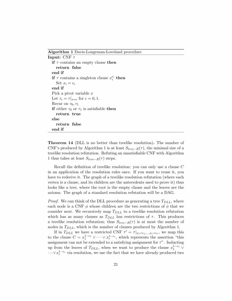
Algorithm 1 Davis-Longeman-Loveland procedure
Input: CNF τif τ contains an empty clause then
return falseend ifif τ contains a singleton clause xεii then
Set xi = εiend ifPick a pivot variable xLet τε = τ |x=ε for ε = 0, 1.Recur on τ0, τ1
if either τ0 or τ1 is satisfiable thenreturn true
elsereturn false
end if
Theorem 14 (DLL is no better than treelike resolution). The number ofCNF’s produced by Algorithm 1 is at least Stree−R(τ), the minimal size of atreelike resolution refutation. Refuting an unsatisfiable CNF with Algorithm1 thus takes at least Stree−R(τ) steps.
Recall the definition of treelike resolution: you can only use a clause Cin an application of the resolution rules once. If you want to reuse it, youhave to rederive it. The graph of a treelike resolution refutation (where eachvertex is a clause, and its children are the antecedents used to prove it) thuslooks like a tree, where the root is the empty clause and the leaves are theaxioms. The graph of a standard resolution refutation will be a DAG.
Proof. We can think of the DLL procedure as generating a tree TDLL, whereeach node is a CNF φ whose children are the two restrictions of φ that weconsider next. We recursively map TDLL to a treelike resolution refutationwhich has as many clauses as TDLL has restrictions of τ . This producesa treelike resolution refutation; thus Stree−R(τ) is at most the number ofnodes in TDLL, which is the number of clauses produced by Algorithm 1.
If in TDLL we have a restricted CNF τ ′ = τ |x1=ε1,...,xr=εr , we map thisto the clause C = x1−ε1
1 ∨ · · · ∨ x1−εrr , which represents the assertion “this
assignment can not be extended to a satisfying assignment for τ”. Inductingup from the leaves of TDLL, when we want to produce the clause x1−ε1
1 ∨· · ·∨x1−εr
r via resolution, we use the fact that we have already produced two
21
children of τ ′ corresponding to different settings of some variable xj . Thismeans that we have produced, via resolution, the two clauses
x0j ∨ x
1−ε11 ∨ · · · ∨ x1−εr
r
x1j ∨ x
1−ε11 ∨ · · · ∨ x1−εr
r .
Applying the resolution rule to these two clauses (with xj being the pivotvariable), we derive the desired clause. (We are using the special case ofresolution C ∨ x,C ∨ x =⇒ C.)
Our base case is the leaves of TDLL, which correspond to restrictions of τwhich violate some clause C of τ . These restrictions are mapped to a clauseC ′ which contains all the variables of C (and possibly others). C ′ can thusbe derived in one step from C (which is part of our input) by the weakeningrule.
It is easy to see that if in Algorithm 1 we do not insist on the par-ticular choice of the pivot variable when τ contains a singleton clause (or,perhaps, even if we do), then the argument becomes reversible. That is,Stree−R(τ) will be precisely the miminal number of clauses generated by anyimplementation of Algorithm 1.
From lecture 2, we know that some CNF’s τ have SR(τ) which is ex-ponential in the number of variables, so Algorithm 1 will not refute themefficiently using any heuristic. We would still like to find a heuristic thatcauses Algorithm 1 to be efficient when τ does have a small refutation. Moregenerally, we would like to efficiently find a proof that is not much longerthan the shortest proof. This motivates the following definition:
Definition 4.1 (Bonet, Pitassi, Raz 2000). A proof system f is automati-zable if there exists an algorithm that outputs an f -proof of any tautologyτ , and runs in time Sf (τ)O(1), i.e., polynomially in the size of the smallestf -proof. (We will let p(Sf (τ)) be this polynomial for future reference.)
A proof system is quasi-automatizable if the same holds, except with aquasi-polynomial time bound.
This property is somewhat weird in that it is not monotone: making aproof system more powerful can make it less automatizable, if we gain theability to make proofs significantly shorter without the ability to find theseshort proofs.
Definition 4.2. A proof system f is normal if
Sf (τ |ρ) ≤ Sf (τ)O(1),
22
i.e., applying a restriction to a CNF does not make it much harder to provein f .
A proof system is strictly normal if
Sf (τ |ρ) ≤ Sf (τ).
i.e., applying a restriction to a CNF does not make it any harder to provein f .
Well-behaved systems will be strictly normal. Resolution is strictly nor-mal, since we can apply ρ to every clause in the proof without invalidatingany of the deductive steps, and possibly making some of them unnecessary.
Recall:
Definition 4.3. A proof system f has feasible interpolation if, given anunsatisfiable CNF τ of the form A(y)∧B(z), and an f -refutation of τ of sizes, we can decide in time sO(1) which of A and B is unsatisfiable. (If neitheris satisfiable, we can answer with either one of them.)
Theorem 15. For any normal proof system f , Automatizability impliesFeasible Interpolation.
This theorem is unfortunate, because we have just proved that, unlessfactoring is easy, we do not have Feasible Interpolation for Extended Frege,Frege, and other nice systems. Thus we do not have Automatizability forthem, either.
Proof. We will only go through the proof for strictly normal proof systems.It is completely straightforward to adapt it to normal proof systems.
Suppose f is automatizable. We then have an algorithm Auto which,given an unsatisfiable CNF τ , outputs a refutation of τ in time p(Sf (τ)). Ifτ is satisfiable, Auto outputs ERROR (without any time restrictions).
We can use Auto to perform feasible interpolation using Algorithm 2.
Claim 4.4. The correctness of Auto ensures that we answer correctly inline 5.
Claim 4.5. If Auto does not finish in p(s) steps (line 3) or outputs some-thing weird (line 7), then B is unsatisfiable.
Suppose B(z) were satisfiable, and let z = b be a satisfying assignment.Then, by strict normality, we have
Sf (A(y) ∧B(z)|z=b) ≤ s = Sf (A(y) ∧B(z))
Sf (A(y) ∧ true) ≤ sSf (A(y)) ≤ s
23
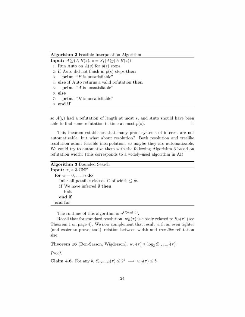
Algorithm 2 Feasible Interpolation Algorithm
Input: A(y) ∧B(z), s = Sf (A(y) ∧B(z))1: Run Auto on A(y) for p(s) steps.2: if Auto did not finish in p(s) steps then3: print “B is unsatisfiable”4: else if Auto returns a valid refutation then5: print “A is unsatisfiable”6: else7: print “B is unsatisfiable”8: end if
so A(y) had a refutation of length at most s, and Auto should have beenable to find some refutation in time at most p(s).
This theorem establishes that many proof systems of interest are notautomatizable, but what about resolution? Both resolution and treelikeresolution admit feasible interpolation, so maybe they are automatizable.We could try to automatize them with the following Algorithm 3 based onrefutation width: (this corresponds to a widely-used algorithm in AI)
Algorithm 3 Bounded Search
Input: τ , a 3-CNFfor w = 0, . . . , n do
Infer all possible clauses C of width ≤ w.if We have inferred ∅ then
Haltend if
end for
The runtime of this algorithm is nO(wR(τ)).Recall that for standard resolution, wR(τ) is closely related to SR(τ) (see
Theorem 1 on page 4). We now complement that result with an even tighter(and easier to prove, too!) relation between width and tree-like refutationsize.
Theorem 16 (Ben-Sasson, Wigderson). wR(τ) ≤ log2 Stree−R(τ).
Proof.
Claim 4.6. For any b, Stree−R(τ) ≤ 2b =⇒ wR(τ) ≤ b.
24
Suppose that τ has a treelike refutation of size less than or equal to 2b.The last deductive step in this refutation will be x, x =⇒ false, and viathe restriction-refutation equivalence for treelike resolution, this implies thatwe have a resolution refutation of τ0 = τ |x=0 and τ1 = τ |x=1. Because ourresolution is treelike, the size of the refutation of τ is the sum of the sizes ofthe refutation of τ0 and the refutation of τ1. Their sum is at most 2b, so oneof them (say τ0) has size at most 2b−1. By induction, we can assume thatwR(τ0) ≤ b− 1 (induction on b), and wR(τ1) ≤ b (an inner induction on thesize of τ). By Lemma 2.3 on page 5, this yields wR(τ) ≤ b, which is whatwe wanted.
Putting this bound together with Algorithm 3, we find that we canfind a resolution refutation for τ in time nO(wR(τ)) = nO(log(Stree−R(τ))) =Stree−R(τ)O(logn). This algorithm is quasi-polynomial, so we are tempted tosay that treelike resolution is quasi-automatizable. This is not true, becausethe refutation produced by Algorithm 3 will not be treelike.
Question 4.7. Neither resolution nor treelike resolution is quasi-automatizable,under any mildly reasonable complexity assumption.
A practical message emerging from all this is that Algorithm 3 is as goodas any DLL procedure, up to a factor of nO(wR(τ)). If you wanted to improvethis to a polynomial factor, you most likely can’t, because:
4.3 Resolution is Probably not Automatizable
Theorem 17 (Alekhnovich Razborov 01). Resolution is not automatizableunless W[P] is tractable.
This shows that automatizability is (most likely) a stronger propertythan feasible interpolation.
This isn’t a class on parameterized complexity, so we do not even attemptto define W[P]. Instead, we indicate a concrete complete problem in thiscomplexity class.
Problem 4.8 (Minimum Weight Monotone Assignment (MWMA)).Instance: C, a monotone circuit on n variables (monotone: using only ∧
and ∨ gates, no negation)Solution: k(C), the minimum Hamming weight of a satisfying assignmenta.
Problem 4.9 (h-Gap MWMA).An algorithm A (receiving as its input a monotone circuit C and an integerk) solves the h-Gap MWMA problem if
25
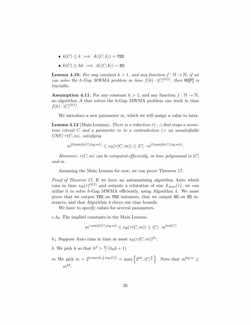
• k(C) ≤ k =⇒ A(〈C, k〉) = YES
• k(C) ≥ hk =⇒ A(〈C, k〉) = NO
Lemma 4.10. For any constant h > 1, and any function f : N→ N, if wecan solve the h-Gap MWMA problem in time f(k) · |C|O(1), then W[P] istractable.
Assumption 4.11. For any constant h > 1, and any function f : N → N,no algorithm A that solves the h-Gap MWMA problem can work in timef(k) · |C|O(1).
We introduce a new parameter m, which we will assign a value to later.
Lemma 4.12 (Main Lemma). There is a reduction τ(·, ·) that maps a mono-tone circuit C and a parameter m to a contradiction (= an unsatisfiableCNF) τ(C,m), satisfying
mΩ(mink(C),logm) ≤ sR(τ(C,m)) ≤ |C| ·mO(mink(C),logm).
Moreover, τ(C,m) can be computed efficiently, in time polynomial in |C|and m.
Assuming the Main Lemma for now, we can prove Theorem 17.
Proof of Theorem 17. If we have an automatizing algorithm Auto whichruns in time sR(τ)O(1) and outputs a refutation of size SAuto(τ), we canutilize it to solve h-Gap MWMA efficiently, using Algorithm 4. We mustprove that we output YES on YES instances, that we output NO on NO in-stances, and that Algorithm 4 obeys our time bounds.
We have to specify values for several parameters.
ε, h0 The implied constants in the Main Lemma:
mεmink(C),logm ≤ sR(τ(C,m)) ≤ |C| ·mh0k(C)
h1 Suppose Auto runs in time at most sR(τ(C,m))h1 .
h We pick h so that h2 > h1ε (h0h+ 1)
m We pick m = 2hmaxk, 1k
log |C| = max
2hk, |C|hk
. Note that mlogm ≥
mhk.
26
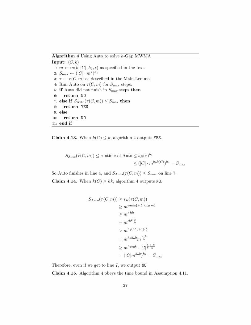
Algorithm 4 Using Auto to solve h-Gap MWMA
Input: 〈C, k〉1: m← m(k, |C|, h1, ε) as specified in the text.2: Smax ← (|C| ·mk)h1
3: τ ← τ(C,m) as described in the Main Lemma.4: Run Auto on τ(C,m) for Smax steps.5: if Auto did not finish in Smax steps then6: return NO
7: else if SAuto(τ(C,m)) ≤ Smax then8: return YES
9: else10: return NO
11: end if
Claim 4.13. When k(C) ≤ k, algorithm 4 outputs YES.
SAuto(τ(C,m)) ≤ runtime of Auto ≤ sR(τ)h1
≤ (|C| ·mh0k(C))h1 = Smax
So Auto finishes in line 4, and SAuto(τ(C,m)) ≤ Smax on line 7.
Claim 4.14. When k(C) ≥ hk, algorithm 4 outputs NO.
SAuto(τ(C,m)) ≥ sR(τ(C,m))
≥ mε·mink(C),logm
≥ mε·hk
= mεh2· kh
> mh1(hh0+1)· kh
= mh1h0kmh1kh
≥ mh1h0k · |C|hk
h1kh
= (|C|mh0k)h1 = Smax
Therefore, even if we get to line 7, we output NO.
Claim 4.15. Algorithm 4 obeys the time bound in Assumption 4.11.
27
The two operations that take superconstant time are creating τ in line 3,and running Auto in line 4. Line 3 takes at most (|C| ·m)O(1), according tothe Main Lemma 4.12. Line 4 takes at most Smax steps, or we stop runningAuto. Since Smax = |C|O(1) · mO(k), and m ≤ 2hk, this results in a timebound of the form |C|O(1) · f(k).
4.3.1 Constructing the contradiction
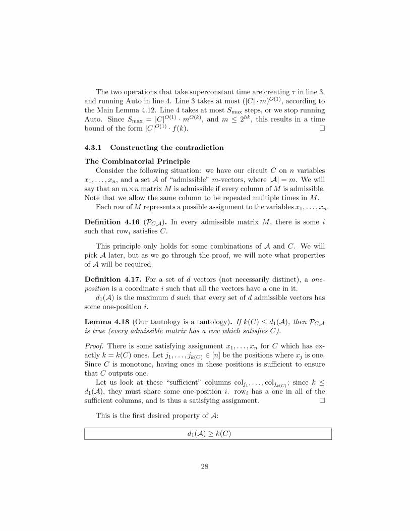
The Combinatorial PrincipleConsider the following situation: we have our circuit C on n variables
x1, . . . , xn, and a set A of “admissible” m-vectors, where |A| = m. We willsay that an m×n matrix M is admissible if every column of M is admissible.Note that we allow the same column to be repeated multiple times in M .
Each row ofM represents a possible assignment to the variables x1, . . . , xn.
Definition 4.16 (PC,A). In every admissible matrix M , there is some isuch that rowi satisfies C.
This principle only holds for some combinations of A and C. We willpick A later, but as we go through the proof, we will note what propertiesof A will be required.
Definition 4.17. For a set of d vectors (not necessarily distinct), a one-position is a coordinate i such that all the vectors have a one in it.
d1(A) is the maximum d such that every set of d admissible vectors hassome one-position i.
Lemma 4.18 (Our tautology is a tautology). If k(C) ≤ d1(A), then PC,Ais true (every admissible matrix has a row which satisfies C).
Proof. There is some satisfying assignment x1, . . . , xn for C which has ex-actly k = k(C) ones. Let j1, . . . , jk(C) ∈ [n] be the positions where xj is one.Since C is monotone, having ones in these positions is sufficient to ensurethat C outputs one.
Let us look at these “sufficient” columns colj1 , . . . , coljk(C); since k ≤
d1(A), they must share some one-position i. rowi has a one in all of thesufficient columns, and is thus a satisfying assignment.
This is the first desired property of A:
d1(A) ≥ k(C)
28
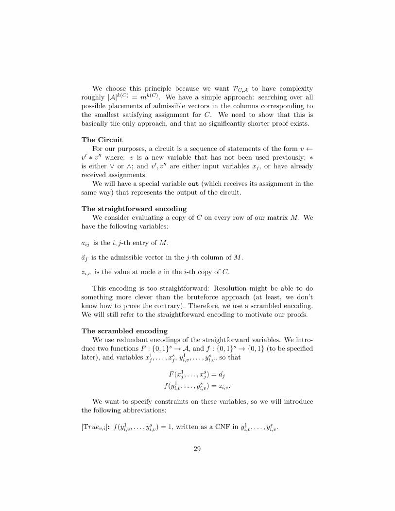
We choose this principle because we want PC,A to have complexityroughly |A|k(C) = mk(C). We have a simple approach: searching over allpossible placements of admissible vectors in the columns corresponding tothe smallest satisfying assignment for C. We need to show that this isbasically the only approach, and that no significantly shorter proof exists.
The CircuitFor our purposes, a circuit is a sequence of statements of the form v ←
v′ ∗ v′′ where: v is a new variable that has not been used previously; ∗is either ∨ or ∧; and v′, v′′ are either input variables xj , or have alreadyreceived assignments.
We will have a special variable out (which receives its assignment in thesame way) that represents the output of the circuit.
The straightforward encodingWe consider evaluating a copy of C on every row of our matrix M . We
have the following variables:
aij is the i, j-th entry of M .
~aj is the admissible vector in the j-th column of M .
zi,v is the value at node v in the i-th copy of C.
This encoding is too straightforward: Resolution might be able to dosomething more clever than the bruteforce approach (at least, we don’tknow how to prove the contrary). Therefore, we use a scrambled encoding.We will still refer to the straightforward encoding to motivate our proofs.
The scrambled encodingWe use redundant encodings of the straightforward variables. We intro-
duce two functions F : 0, 1s → A, and f : 0, 1s → 0, 1 (to be specifiedlater), and variables x1
j , . . . , xsj , y
1i,v, . . . , y
si,v, so that
F (x1j , . . . , x
sj) = ~aj
f(y1i,v, . . . , y
si,v) = zi,v.
We want to specify constraints on these variables, so we will introducethe following abbreviations:
[Truev,i]: f(y1i,v, . . . , y
si,v) = 1, written as a CNF in y1
i,v, . . . , ysi,v.
29
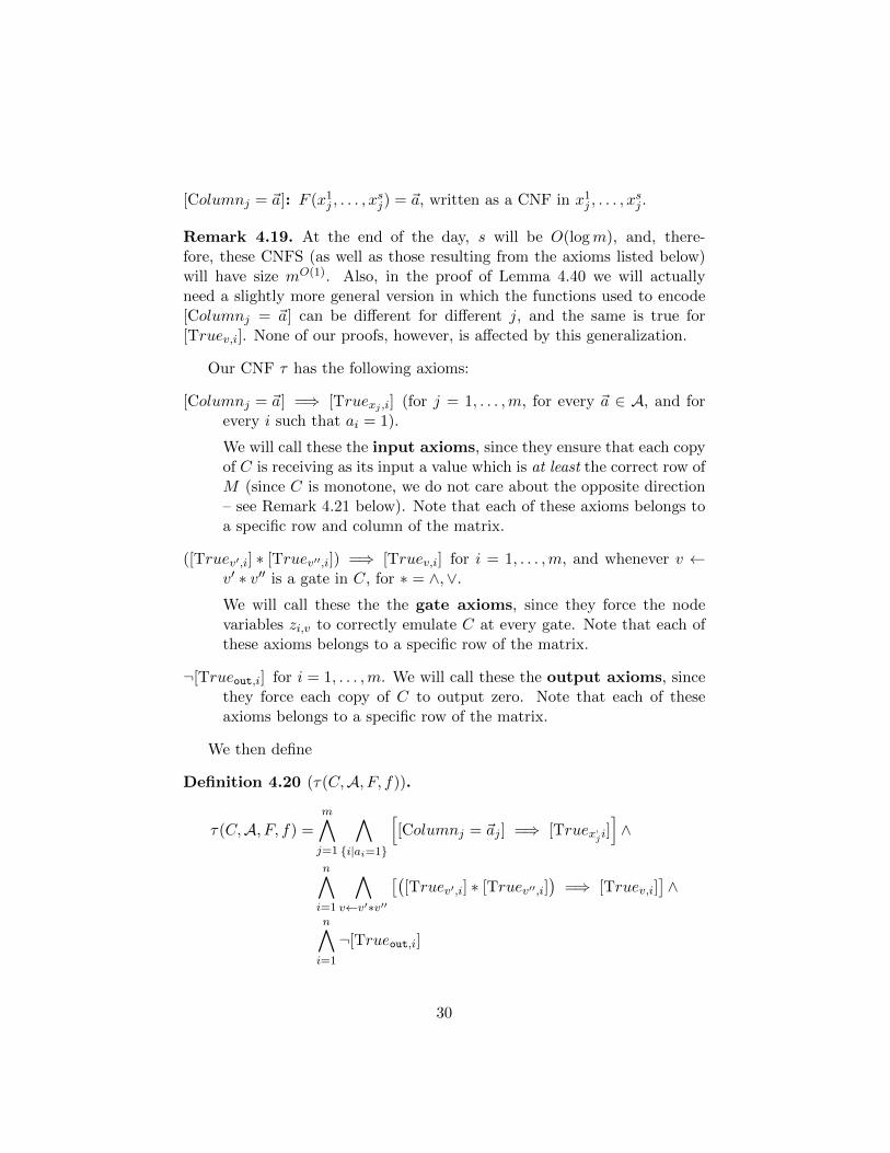
[Columnj = ~a]: F (x1j , . . . , x
sj) = ~a, written as a CNF in x1
j , . . . , xsj .
Remark 4.19. At the end of the day, s will be O(logm), and, there-fore, these CNFS (as well as those resulting from the axioms listed below)will have size mO(1). Also, in the proof of Lemma 4.40 we will actuallyneed a slightly more general version in which the functions used to encode[Columnj = ~a] can be different for different j, and the same is true for[Truev,i]. None of our proofs, however, is affected by this generalization.
Our CNF τ has the following axioms:
[Columnj = ~a] =⇒ [Truexj ,i] (for j = 1, . . . ,m, for every ~a ∈ A, and forevery i such that ai = 1).
We will call these the input axioms, since they ensure that each copyof C is receiving as its input a value which is at least the correct row ofM (since C is monotone, we do not care about the opposite direction– see Remark 4.21 below). Note that each of these axioms belongs toa specific row and column of the matrix.
([Truev′,i] ∗ [Truev′′,i]) =⇒ [Truev,i] for i = 1, . . . ,m, and whenever v ←v′ ∗ v′′ is a gate in C, for ∗ = ∧,∨.
We will call these the the gate axioms, since they force the nodevariables zi,v to correctly emulate C at every gate. Note that each ofthese axioms belongs to a specific row of the matrix.
¬[Trueout,i] for i = 1, . . . ,m. We will call these the output axioms, sincethey force each copy of C to output zero. Note that each of theseaxioms belongs to a specific row of the matrix.
We then define
Definition 4.20 (τ(C,A, F, f)).
τ(C,A, F, f) =m∧j=1
∧i|ai=1
[[Columnj = ~aj ] =⇒ [Truex,ji]
]∧
n∧i=1
∧v←v′∗v′′
[([Truev′,i] ∗ [Truev′′,i]
)=⇒ [Truev,i]
]∧
n∧i=1
¬[Trueout,i]
30
Remark 4.21. As we already indicated above, we are allowing assignmentsto cheat in one direction: in terms of the straightforward encoding, we areallowing (zi,xj = 1 ∧ aij = 0) and (zi,v′ ∗ zi,v′′ = 0 ∧ zi,v = 1). This does notcause problems: we claim that any satisfying assignment for τ(C,A, F, f)would produce a genuine counterexample to PC,A.
We can produce this counterexample by setting zi,xj = 0 whenever aij =0, and then repeatedly changing zi,v to zero when its children would make itzero in C. Since C is acyclic and monotone, this will eventually correct allerrors of the two forms we allow. Since we never change any variable fromzero to one, this cannot cause any copy of C to be satisfied.
Thus, (the negation of) τ(C,A, F, f) is equivalent to PC,A. Allowing thischeating gives us some needed flexibility later in the proof.
Lemma 4.22. We can efficiently construct a CNF encoding of τ(C,A, F, f)as long as we can efficiently compute F, f , and as long as we can efficientlyenumerate A. (Here efficiently means in time polynomial in |C| and m.)
Exercise: Prove this.
4.3.2 The Upper Bound on sR
Lemma 4.23. If k(C) ≤ d1(A), then sR(τ(C,A, F, f)) ≤ O(|C|·2s(k(C)+1)).
Proof. There is some satisfying assignment x1, . . . , xn for C which has ex-actly k(C) ones. Let J1 = j1, . . . , jk(C) be a set of columns where xj is one.We then use the Canonical Refutation in Algorithm 5 on these columns.
We can find an appropriate i in line 3 because |J | ≤ d1(A). We cansuccesfully deduce [Trueout,i] in line 7 because (∀j ∈ J1, xj = 1) =⇒C(x1, . . . , xn) = 1.
Exercise: Show that the Canonical Refutation can be encoded in a Resolu-tion refutation using O(|C| · 2s(k(C)+1)) clauses.
Remark 4.24. Theorem 17 is also true for tree-like resolution, but theproof is more complicated. The reason is that since C is a circuit ratherthan a formula, the Canonical Refutation need not necessarily be tree-like.This problem is fixed by introducing an even more elaborate encoding (seethe paper for the details).
31
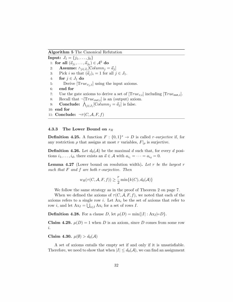
Algorithm 5 The Canonical Refutation
Input: J1 = j1, . . . , jk1: for all (~aj1 , . . . ,~ajk) ∈ Ak do2: Assume: ∧j∈J1 [Columnj = ~aj ]3: Pick i so that (~aj)i = 1 for all j ∈ J1.4: for j ∈ J1 do5: Derive [Truexj ,i] using the input axioms.6: end for7: Use the gate axioms to derive a set of [Truev,i] including [Trueout,i].8: Recall that ¬[Trueout,i] is an (output) axiom.9: Conclude:
∧j∈J1 [Columnj = ~aj ] is false.
10: end for11: Conclude: ¬τ(C,A, F, f)
4.3.3 The Lower Bound on sR
Definition 4.25. A function F : 0, 1s → D is called r-surjective if, forany restriction ρ that assigns at most r variables, F |ρ is surjective.
Definition 4.26. Let d0(A) be the maximal d such that, for every d posi-tions i1, . . . , id, there exists an ~a ∈ A with ai1 = · · · = aid = 0.
Lemma 4.27 (Lower bound on resolution width). Let r be the largest rsuch that F and f are both r-surjective. Then
wR(τ(C,A, F, f)) ≥ r
2mink(C), d0(A)
We follow the same strategy as in the proof of Theorem 2 on page 7.When we defined the axioms of τ(C,A, F, f), we noted that each of the
axioms refers to a single row i. Let Axi be the set of axioms that refer torow i, and let AxI =
⋃i∈I Axi for a set of rows I.
Definition 4.28. For a clause D, let µ(D) = min|I| : AxI |=D.
Claim 4.29. µ(D) = 1 when D is an axiom, since D comes from some rowi.
Claim 4.30. µ(∅) > d0(A)
A set of axioms entails the empty set if and only if it is unsatisfiable.Therefore, we need to show that when |I| ≤ d0(A), we can find an assignment
32
that satisfies AxI . Since |I| ≤ d0(A), some ~a ∈ A has (~a)i = 0 for all i ∈ I.We can then satisfy AxI by setting
M = [~a · · ·~a] (1)
zi,v = 0 for i ∈ I (2)
In the I rows, all variables are zero, which is consistent with the gate andoutput axioms. The input axioms are satisfied because ~a is also zero in theserows.
Claim 4.31 (“Continuity of µ”). In the deduction
D1 D2
D,
µ(D) ≤ µ(D1) + µ(D2). This is because I1|=D1, I2|=D2 =⇒ I1 ∪ I2|=D.
Definition 4.32. An intermediate clause is a clause D satisfying
1
2d0(A) ≤ µ(D) ≤ d0(A).
Claim 4.33. R can be rewritten so that it contains an intermediate clauseD.
Consider the set of clauses in R which satisfy condition c: µ(D) <12d0(A). The conclusion (∅) does not, so there must be a first clause Dwhich violates c. D cannot be an axiom, so it must have been derived.
If D was derived using the resolution rule on clauses D1 and D2, thenD1 and D2 appear before D, and thus satisfy c. By the continuity property,µ(D) ≤ 1
2d0(A) + 12d0(A) = d0(A).
If D was derived through weakening, then it was derived from some D1
that satisfies c. We can then break the weakening into two steps, D1 =⇒D′ =⇒ D, where D′ is an intermediate clause.
Claim 4.34. If D is an intermediate clause, it cannot satisfy both
wR(τ(C,A, F, f)) <r
2k(C) (3)
wR(τ(C,A, F, f)) <r
2d0(A) (4)
Let I be a set realizing the minimum |I| : AxI |=D. If we remove anyelement i0 ∈ I, we will get a set I ′ for which ¬(AxI′ |=D). This means thatthere is some assignment xtj = αtj , y
ti,v = βtj that satisfies AxI′ but violates
D.
33
Claim 4.35. We can modify this assignment to satisfy AxI , without mod-ifying any variable that appears in D. (Thus continuing to violate D.)
How would we build such an assignment? We want to modify α, β tosatisfy Axi0 without messing up any of the other rows. Our goal is to achievethe following assignment to the straightforward variables:
• Set the ~aj to be zero in all of I in any column j where this is possiblewithout modifying D’s variables. We will say that a column is free iswe can put any ~a there without disturbing D. We will say that theother columns are fixed.
• Leave the zi,v alone for i ∈ I ′.
• We will set the zi0,v as they would be while correctly emulating C onthe input ~x0 which is one in fixed columns and zero in free columns.We will say that a row is free if we can set the zi0,v arbitrarily withoutdisturbing D.
All that remains is to choose a free row i0, and to prove that mostcolumns are free. Let wi(D) be the number of yti,v that appear in D. Let
wj(D) be the number of xtj that appear in D.We choose i0 to minimize wi(D), so that we have maximum freedom
to change this row’s variables without disturbing D. By the r-surjectivityof f , a row i is free if at most r of the y1
i,v, . . . , ysi,vappear in D. We have∑
iwi(D) ≤ w(D) < r2d0(A), and
∑iwi(D) ≥
∑i∈I wi(D) ≥ |I|wi0(D).
Since |I| ≥ 12d0(A), we have wi0(D) ≤ r, and thus i0 is a free row.
By the r-surjectivity of F , a column is free if D contains at most r of thex1j , . . . , x
sj . We have
∑j w
j(D) ≤ w(D) < r2k(C). Let J0 = j | wj(D) > r.
Then r · |J0| ≤∑
j wj(D), so |J0| < 1
2k(C). Thus any column outside of J0
is free.
Claim 4.36. For any free column j /∈ J0, we can choose α to set (~aj)i = 0simultaneously for all i ∈ I, without disturbing D.
Since |I| ≤ d0(A), there is an admissible vector ~a satisfying this condi-tion. We can then put ~a in any free column by modifying α.
Claim 4.37. We can choose β to set rowi to ~x0 without disturbing D.
Claim 4.38. The input axioms from AxI are satisfied by α, β.
Claim 4.39. The gate and output axioms from Axi0 are satisfied by α, β.
34
Proof. We have modified the yti0,v to make the zi0,v correctly emulate Crejecting input ~x0.
This completes the proof of Claim 4.34 and hence of the width lowerbound, but we are more interested in a lower bound on the size of the proof:
Lemma 4.40 (Lower bound on resolution size). sR(τ(C,A, F, f)) ≥ eΩ( r2
s·mink(C),d0(A)).
The naive way to try to deduce it from Lemma 4.27 would be to applythe general trade-off between width and size (Theorem 1 on page 4). Un-fortunately, the parameters do not work out nicely (or at least we do notknow how to make them work). Instead, we are using the method of randomrestrictions (later on we will see its much more elaborated version).
All our variables are split into blocks Xj , Yiv according to their sub-scripts, s variables in each block. Let us choose independently at random(r/2) variables in each block and assign them to 0, 1 (also independently atrandom). What will happen to our refutation? The first nice thing is thatevery individual fat clause will be eliminated with high probability.
Lemma 4.41. For a clause C with w(C) ≥ r4 mink(C), d0(A), the proba-
bility it is not eliminated by a random restriction is at most e−Ω( r2
s·mink(C),d0(A)).
Exercise: Prove this.And then, since we have assigned just (r/2) variables in each block,
F |ρ, f |ρ will still be (r/2)-surjective (although they can become different ineach block – cf. Remark 4.19!). So, we will get a refutation of a contradictionthat still has the form τ(C,A, F |ρ, f |ρ), and we can apply to it Lemma 4.27to conclude that in fact not all fat clauses have been eliminated. Comparingthis with Lemma 4.41 and applying the union bound completes our proof.
4.3.4 Combinatorial Voodoo
For a matrix A, we define d1(A) (d0(A)respectively) to be the maximumnumber of columns (rows, resp.) such that there is some row (column, resp.)which contains only ones (zeros, resp.) in the intersection of the row andcolumns. For our proof, we need a 0-1 matrix A such that d1(A), d0(A) ≥Ω(logm). Explicit examples of such matrices are well-known, e.g.:
Definition 4.42 (The Paley Matrix). Let m be a prime, and, for i, j ∈ Fm,aij = iff j 6= i and (j − i) is a quadratic residue mod m.
35
F and f need to be r-surjective functions on s bits, where s and rare Θ(logm). For this, we use linear codes. Let h be a sufficiently largeconstant and L ⊆ 0, 1h log2m be an F2-linear subspace of dimension logmthat does not contain non-zero vector of weight < logm. There are manyexplicit examples of such L. Now, fix in L an arbitrary basis x1, . . . , xlogm,and let F : 0, 1h logm → 0, 1logm be the linear mapping defined byF (y) = (〈x1, y〉, . . . 〈xlogm, y〉). Then F is (logm)-surjective.
4.3.5 The Upper Bound when k(C) is too large
Choosing s = Θ(logm), we have proved that
mΩ(mink(C),logm) ≤ sR(τ(C,A, F, f)) ≤ O(|C| ·mO(k(C))).
We still need to prove that sR(τ) ≤ |C| ·mO(logm). Our construction thusfar cannot possibly supply this, since we have been assuming all along thatk(C) ≤ d1(A). When k(C) > d1(A), it is even possible that τ(C,A, F, f) issatisfiable.
We need explicit examples of unsatisfiable CNF’s with sR(τm) = mΘ(logm).We note that the Tseitin tautologies provide τt with sR(τt) = 2Θ(t), so if wetake t = (logm)2, these will suffice.
We define τ(C,m) = τ(C,A, F, f) ∧ τm, where the τm is operating oncompletely new variables. Now resolution can choose between disprov-ing τ(C,A, F, f) and disproving τm, so we have sR(τ(C,m)) ≤ sR(τm) ≤mO(logm).
Our lower bound is still valid because of feasible interpolation. If we havea refutation for τ(C,A, F, f) ∧ τm of size s, then we must have a refuationof size sO(1) for τ(C,A, F, f) or τm. This will only weaken the constant insR(τ(C,m)) ≥ mΩ(mink(C),logm).
This completes the proof of the Main Lemma, and thus the theorem.
Lectures 12 and 13Scribe: Gabriel Bender, University of Chicago.
Date: February 17 and 19, 2009
5 Applications to Learning
Definition: k(C) is the minimum number of ones in a satisfying assignmentof a circuit C.
36
PAC (“Probable, Approximate, Correct”) is a model in learning theoryin which we want to learn from examples generated randomly by naturewith an unknown distribution D.
• Input: A list of pairs (x1, f(x1)), . . . , (xn, f(xn)) for an unknown func-tion f generated accordingly to D.
• Output: A circuit C that will perform “reasonable well” in tryingto predict the output of f on future inputs according to the samedistribution.
“Exact Learnability” is a simple model which (under certain conditionsthat are always fulfilled in our situation) implies PAC learnability.
Definition: Given 0, 1n, a Concept Class is a class of Boolean ex-pressions C which represents Boolean functions f : 0, 1n → 0, 1. Forinstance, C could be the set of all DNFs in n variables.
5.1 Decision Trees
One concept class of particular interest is the set of all decision trees underthe following construction:
Definition: A decision tree in n variables is a binary tree in which everynode has a label, as well as two edges labeled 0 and 1, and every leaf islabeled “accept” or “reject.”
Definition: A decision tree is balanced if every leaf is at the same depth.
Definition: The height of a tree, h(T ), is the length of the maximal pathfrom the root to any leaf.
Problem: Given a system of equations F (a1) = ε1, . . . , F (am) = εm, wewould like to solve it in the concept class C consisting of all decision trees.That is, we want to find F ∈ C that satisfies F (ai) = εi for 1 ≤ i ≤ m. Wewould like to do this as efficiently as possible, and want our solution to be“not much longer” than the size s of the minimal solution F ∈ C.
Definition: By proper learning theory, we mean (as above) that an outputhypothesis F must be in the same concept class as our original function F .
37
Theorem 18 (Alekhnovich et al.). DNF formulas of size s can be exactlylearned in time mO(1)nO(
√n log s). Notice that this is subexponential, but not
polynomial-time.
Theorem 19. Decision trees are not PAC-learnable in polynomial timeunless SAT is computable in randomized time which is subexponential.
Proof of Theorem 18: This proof has close parallels to the proof that“Short proofs are narrow” (Theorem 1 on page 4). We replace wR(P ), therefutation width of a proof tree P , with the “fanning” width of a DNF ex-pression, ie. the maximum number of variables that appears in any of itsterms. In the original analysis of proof trees, a clause C was fat if w(C) > dfor some predetermined d. Here, a term is fat if it involves at least d variables.
Induction Base: Assume our system S has a solution without fat terms.Then we claim that there exists an algorithm BoundedSearch(S) that solvesthe problem in allocated time. Since there are no fat clauses, each expressionhas at most d variables. Hence, there are at most O(n)d possible terms. Wesimply take, in the allotted time, all those terms that are consistent with allnegative examples F (a) = 0, and check if they “cover” all positive examplesF (a) = 1.
Inductive step: Suppose we have f fat clauses. In the proof of Theorem1, we took 2n restrictions. By the Pigeon-Hole Principle, one of those restric-tions was guaranteed to produce at most αf fat clauses, where α = (1− 2d
n ).However, when we try to apply that approach here, we run into trouble be-cause we don’t know which restriction will sufficiently simplify our system.The solution is to run our algorithm recursively on all 2n restrictions inparallel:
Algorithm: Search(S): Run the following restrictions in parallel:
Search(S |x1=0), Search(S |x1=1), . . . ,Search(S |xn=1)
We wait for at least one search to terminate. Assume W.L.O.G. that it isthe restriction xi = ε. Let T (n, f) denote the amount of time needed to finda solution with n variables and f fat clauses. Then T (n, f) satisfies T (n, 0) ≤nO(√n log s)mO(1) by the base case. Furthermore, T (n, f) ≤ (2n)T (n, αf) +
T (n−1, f). T (n, αf) represents the time needed to run the search algorithmon our “good” restriction xi = ε. The time is multiplied by 2n because we’rechecking all 2n possible restrictions in parallel. Once one of our searches has
38
terminated, we need to run the algorithm on the complementary restrictionxi = 1− ε; this accounts for the additional term T (n− 1, f).
The fact that, despite the extra 2n term, this recursion still resolves toT (n, s) ≤ mO(1)nO(
√n log s) is in Homework # 2.
6 Concrete Lower Bounds
Let Fd denote the depth-d Frege system (in which every clause has depth atmost d). Then we know that
F1 ≤ Res(k) ≤ F2
(recall that Res(k) is the natural proof system operating with k-DNFs).
6.1 Random 3-CNFs
Suppose we have a CNF τ with n variables and Cn clauses chosen at ran-dom. If C is big then τ is almost surely unsatisfiable. We may thereforeask: what is the minimum refutation size in various proof systems?
Extended Frege: We believe that SEF (τ) ≥ exp(nΩ(1)). Intuitively, thismeans you can’t do much better for random 3-CNFs than a brute-forcesearch through solutions. But the strongest system for which we can reallyprove this is Res(k):
Theorem 20 (Alekhnovich 05). SRes(√
logn/log logn)≥ exp(nΩ(1)).
6.2 The Pigeon-Hole Principle
We introduce the notation: [m] = 1, 2, . . . ,m for an integer m.
Observation: Let our domain D = [m] and our range R = [n]. If m > nthen there is no bijection from [m] to [n].
We create Pigeon-Hole contradiction as follows:
• For each i ∈ [m], j ∈ [n], we introduce a new variable xij . Intuitively,this corresponds to the statement “Pigeon i is in hole j.”
• For each i ∈ [m], we set Qi =∨nj=1 xi,j . Intuitively, Qi represents the
statement “Pigeon i is in some hole.”
39
• For j ∈ [n] we let Qj represent the statement “Hole j contains somepigeon:” Qj =
∨ni=1 xi,j
• For each i1 6= i2 ∈ [m] and j ∈ [n], Qi1,i2,j = xi1,j ∨ xi2,j . Thiscorresponds to the statement “no two pigeons share the same hole.”
• For each i ∈ [m] and j1, j2 ∈ [m], we set Qi,j1,j2 = xi,j1 ∨ xi,j2 . Thisrepresents the statement “no pigeon is placed in two (or more) holes.”
Definitions: Let i, i1, i2 ∈ [m] and j, j1, j2 ∈ [n]. We define the followingCNFs by listing their sets of clauses:
• PHPmn = Qi ∪ Qi1,i2,j
• FPHPmn = PHPmn ∪ Qi,j1,j2
• onto-PHPmn = PHPmn ∪ Qj
• onto-FPHPmn = FPHPmn ∪ Qj
Theorem 21 (Maciel, Pitassi, Woods 99). SRes((logn)O(1))(PHP2nn ) ≤ nO(logn).
It is an open question whether we can say the same thing about Res(2).
Theorem 22 (Krajicek, Pudlak, Woods, Pitassi, Beame, Impagliazzo 93).SFd
(onto-FPHPn+1n ) ≥ exp(nεd) with a constant εd > 0.
Theorem 23 (Raz, Razborov 01). SR(onto-FPHP∞n ) ≥ exp(Ω(n1/3))
There is a number of interesting problems about the complexity of PHPthat are still open (see the course Web page).
6.2.1 Matching Restrictions
Suppose ρ is a restriction. Let m = n + 1 and l = nε. Then MlD×R is the
set of partial matchings assigning pigeons to all but l holes.Formally, we start with a collection of pairs (iν , jν). We say that
ρ(xij) =
1, if i = iν and j = jν for some ν0, if i = iν for some ν and j 6= jν0, if j = jν for some ν and i 6= iν
40
6.2.2 Matching Decision Trees
A Matching Decision Tree is a tree. At each node, we can either query apigeon i or we can query a hole j. If we query the node of a pigeon i then oneof the variables xi,1, . . . , xi,n will be 1. Hence, our “pigeon” node will haven successors corresponding precisely to those variables. The intermediateedges will have the labels j = 1, . . . , j = n respectively.
Similarly, if we query a hole j then we can determine which of m pigeonsx1,j , . . . , xm,j sits in it. Hence, a “hole” node will have m successors withedges labeled i1, . . . , im, corresponding to the cases xi,1 = 1, . . . , xi,m = 1respectively.
All leaves in the decision tree are labeled by 0 or 1. Let Br(T ) denote theset of all leaves, Br0(T ) be the set of leaves labeled by 0, and Br1(T ) be theset of leaves labeled by 1. Every leaf naturally corresponds to a matchingrestriction.
Definition: A matching decision tree T represents F if
• (∀ρ ∈ Br0(T ))(F ρ≡ 0)
• (∀ρ ∈ Br1(T ))(F ρ≡ 1)
6.2.3 Putting it all together
Define h(T ) to be the maximum length over all paths from the root of T toany node.
As a first attempt, we might say that all formulas can be represented bylow-height matching decision trees with only accepting branches. However,this fails for the depth-2 formula that is the conjunction of axioms: it iseasily deducible but never accepts.
More specifically, let (∧iQi) ∧ (
∧i1,i2,j
Qi1,i2,j) be the conjunction of allof the PHPmn axioms. It is a depth-2 formula, and is identically zero in thereal world, since there are more pigeons than holes in our setup.
Let Γ be a set of all subformulas that appear in our proof P .
Definition Consider the set of formulas over the language consisting ofthe constants 0, 1 and the operators ¬ and ∨. The k-evaluation is a map
41
F 7→ TF that takes formulas to matching decision trees of height at most k.It is defined as follows:
• T0 consists of a tree with a single node labeled 0, ie. always reject
• T1 consists of a tree with a single node labeled 1, ie. always accept
• T¬F ≡ T cF , ie. take the tree TF and reverse all the labels.
• F =∨i∈I Fi. We wish to express TF in terms of the TFi values. Ideally
we would like to let TF represent∨i∈I Disj (TFi), where Disj (T ) =∨
ρ∈Br1(T ) tρ is a matching disjunction; tρ ≡∧i∈dom(ρ) xi,ρ(i).
We will discuss how to construct a k-evaluation later. For the time beinglet us notice that it suffices for our purposes.
Lemma 6.1. Suppose k < n3 . Assume Γ is an arbitrary set of formulas that
is closed under subformulas and that has a k-evluation. Then there is norefutation of the Pigeon-Hole Principle in which all lines belong to Γ.
Lectures 14 and 15Scribe: Paolo Codenotti, University of Chicago.
Date: February 24 and 26, 2009
Let us finish the discussion on how to construct k-evaluations. Let Γbe a set of formulas closed under subformulas. Let Γi ⊆ Γ be the set offormulas in Γ of depth at most i. So we have
Γ0 ⊆ Γ1 ⊆ Γ2 ⊆ · · · ⊆ Γd = Γ.
By induction, we will construct ki-evaluations for Γi|ρi , where ρi are restric-tions we will construct as we go along, with ρi+1 an extension of ρi.
It is easy to see that restrictions are a natural and robust concept. Inparticular this means that Γi|ρi+1 will still be a ki-evaluation, independentlyof our choice of ρi+1 (since ρi+1 extends ρi). The only case we need to takecare of is when F =
∨i∈I Fi, where the Fi are already evaluated formulas.
In particular, we have F =∨i∈I ti, where the ti are matching terms with at
most r variables. We can assume without loss of generality that ρi is trivial(since we can assume it is already fixed). In order to finish our construction,and show we can get a restriction ρi+1 for which we can get ki+1-evaluationsfor some small ki+1, we use the following lemma.
42
Lemma 24 (Switching Lemma). Let F be a matching r-disjunction, andlet 10 ≤ ` ≤ ε
√n/r, where ε is a constant (something like 1/10). Let ρ be
a random restriction that assigns all but ` + 1 pigeons. Then F |ρ can berepresented by a height s matching decision tree with probability at least1− exp (−Ω(`2
√r/n))s.
In a slightly different context, this lemma was first stated and proved byHastad in 1986. A simple combinatorial proof was given 10 years later byRazborov.
Once we have Lemma 24, the proof is completed by a simple applicationof the union bound: for every individual F ∈ Γd \Γd−1, the probability thatF |ρk+1
does not get simplified as necessary is |Γd|−1.
7 Algebraic and Geometric proof systems
Assignments to formulas are points on the boolean cube. There are twoways to translate formulas so that variables become numbers (i.e. elementsof some field K). The two schools of thought differ in how clauses arerepresented.
1. In the algebraic approach clauses are represented by equations.
2. In the geometric approach clauses are represented by inequalities.
Let us show how this is done by example. The clause x1 ∨ x2 ∨ x3 canbe written as (1− x1)x2(1− x3) = 0 (algebraic), or x1 + (1− x2) + x3 ≥ 1,which simplifies to x1 + x3 ≥ x2 (geometric).
7.1 Algebraic proof systems
We will have the axioms x2i − xi = 0 (which force xi = 0, 1). This means
that we considerΛn = K[x1, . . . , xm]/(x2
i − xi),
which is a ring of multilinear polynomials over our field K.
7.1.1 Nullenstellensatz proof systems
A CNF reduces to a system of polynomial equations f1 = 0, . . . , fm = 0. Itis easy to see that there is no solution to the above system of equations ifand only if there exist polynomials Qi such that
1 = Q1f1 + · · ·+Qmfm
43
(note that due to the presence of the axioms x2i − xi = 0, we do not have to
require that the field K is algebraically closed). Therefore the polynomialsQi are a refutation for the CNF. This is called the Nullstellensatz proofsystem. The degree of a refutation is defined as
d(1 = Q1f1 + · · ·+Qmfm) = maxi
deg (Qi).
We define dKNS(τ) to be the minimum degree of any refutation of a polyno-mial translation of τ .
7.1.2 Polynomial Calculus
Polynomial Calculus(PC) is a proof system that is a ”dynamical version” ofNullstellensatz. The inference rules in Polynomial Calculus are the following:
f = 0 g = 0
αf + βg = 0∀α, β ∈ K
f = 0
f · xi = 0∀i ∈ [n]
We define the degree of the first rule to be maxdeg(f),deg(g), and thedegree of the second rule to be deg(f) + 1. A PC refutation is a sequenceof inferences proving 1 = 0. The degree of a refutation of a contradiction τis dKPC(τ), the minimum degree of a PC refutation of τ . We can make thefollowing two observations about dKPC(τ):
• dKPC(τ) ≤ wR(τ) (we can simulate resolution rules with polynomialcalculus).
• dKPC(τ) ≤ dKNS(τ) +O(1).
There are many separation results for Polynomial Calculus and Nullstel-lensatz. For example Buss and Pitassi showed the following.
Theorem 25 (Buss, Pitassi 1998). Let τ be the least induction principle.x1 = 1, xi ⇒ xi+1, xn = 0. τ is obviously unsatisfiable and has a PCrefutation of degree 2 (or 3). However, dKNS(τ) is linear in n over any field.
Proposition 7.1. PC refutations of degree O(1) are automatizable (see lec-ture 9 for the definition).
Proof. The proof is essentially the Groebner basis algorithm. The idea is asfollows. Let Xd be the linear space of polynomials of degree d you can infer.We iteratively look at all polynomials we can infer in the set of polynomialsof degree d + 1, and intersect it back with the set of polynomials of degreed.
44
Efficient Interpolation Property: As a corollary, PC refutations ofconstant degree have the efficient interpolation property. That is, let τ =τ ′, τ ′′ = τ ′(x, y), τ ′′(x, z) be unsatisfiable with dKPC(τ) ≤ O(1). Then, givenx, we can point out in polynomial time which of τ ′ and τ ′′ is not satisfiable.
Polynomial Calculus with Resolution: We would like our system tohave the property that terms and their negations have the same size. How-ever, this is far from true in PC: the negation of the clause x1 · · · · · xn is(1 − x1)(1 − x2) . . . (1 − xn), which has much larger size, even though thedegree is the same. Polynomial Calculus with Resolution (PCR) solves thisproblem. In PCR, we allow linear combinations of all clauses. Note thatdPC = dPCR. To prove lower bounds for PCR, we can follow the same strat-egy as in proving lower bounds for resolution. In particular, we can take aPCR proof, hit it with a random restriction, this kills all fat clauses, so weend up with a PCR refutation of low degree, and then we prove that such athing does not exist. Since the degree of PCR is the same as the PC degree,lower bounds on the PC degree are the key for lower bounds for PCR.
Lower Bounds for PC Refutations for which PC lower bounds areknown include the following:
• Random CNF (Ben-Sasson, Impagliazzo, 99).
• Pigeon Hole Principle (PHP):
Theorem 26 (Razborov, 95).
dkPC(PHPmn ) ≥ n/2.
The proof technique is the ”pigeon dance.”
• Tsetin tautologies: we will prove the following result in class.
Theorem 27 (Buss, Grigoriev, Impagliazzo, Pitassi, 99).
char(K) 6= 2⇒ dKPC(τ(G, f)) ≥ e(G)/2.
Recall from lecture 2 the definition of Tsetin Tautologies, and edge ex-pansion. Given a graph G on n vertices, and a function f : V (G)→ 0, 1such that ⊕v∈V (G)f(v) = 1. Let xe | e ∈ E(G) be the set of variables. TheTsetin tautology is defined as τ(G, f) ≡ (∀v ∈ V (G))(⊕e3vxe = f(v)). the
45
edge expansion of a graph is e(G) = minn/3≤|V |≤2n/3 |E(G) ∩ (V × co-V )|.Recall the Ben-Sasson, Wigderson result from lecture 2:
wR(τ(G, f)) ≥ e(G).
Proof of Theorem 27. The overall strategy of the proof is the following:
dKPC(τ(G, f)) ≥ wg(τ(G, f))/2 ≥ wR(τ(G, f))/2 ≥ e(G)/2.
Here wg(τ) is the Gaussian width: the width of a refutation using the rule
f = ε g = δ
f ⊕ g = ε+ δ, ε, δ ∈ 0, 1
Note that τ(G, f) is a system of linear equations mod 2. We will showthat for any system of linear equations mod 2, dKPC(τ) ≥ wg(τ)/2 ≥ wR(τ)/2.The Ben-Sasson, Wigderson result from lecture 2 will conclude the proof.
In fact, it is known that wg(τ) = wR(τ), but we will only show theinequality required in the proof (wg(τ) ≥ wR(τ)). The other direction isleft as homework. Given a Gaussian refutation, we want to construct aresolution refutation of the same width. We will achieve this by encodingeach equation in the Gaussian refutation by clauses. Given an equationx1 ⊕ x2 ⊕ x3 = 0, we can encode this by 4 clauses: (x1 ∨ x2 ∨ x3), (x1 ∨x2 ∨x3), (x1 ∨x2 ∨x3), (x1 ∨x2 ∨x3). Clearly this transformation preserveswidth, and applying this encoding line by line to a Gaussian refutation, weobtain a resolution refutation.
We are left to show that dKPC(τ) ≥ wg(τ)/2 for any system of linearequations mod 2. We will switch from additive to multiplicative notation.In particular our variables xi ∈ 0, 1 will correspond to variables yi ∈−1, 1. Note that we make key use of the fact that char(K) 6= 2. Thetransformation is as follows:
xi →1− yi
2(yi = exp(iπxi))
x1 ⊕ x2 ⊕ · · · ⊕ x` = ε → y1y2 . . . y` = ε′
x2i = xi → y2
i = 1.
The main idea of the proof is about binomials. Consider a binomial b ofthe form m1±m2, where m1 and m2 are monomials. Since for any monomialm, m2 = 1, we have:
m1 ±m2 = 0 ⇐⇒ m1m2 = ±1
46
Therefore by reversing the map back to the xi, we can associate a linearequation mod 2 to every binomial.
Given a PC refutation P of degree at most d, our goal is to constructa Gaussian refutation of degree at most 2d. Let f ∈ P , our goal will beto show that we can write f in the form f = α1b1 + · · · + αtbt, wheredeg(bi) ≤ d, and every bi has a binomial (i.e., the one in which every lineis a binomial) proof from our binomial axioms. Once we have this, it is anobvious exercise to prove that we have a Gaussian refutation of degree atmost 2d, since deg(m1m2) ≤ 2d.
We will prove by induction on f the following. Given f such thatdeg(f) ≤ d0 ≤ d, we can write f as f = α1b1 +· · ·+αtbt, where deg(bi) ≤ d0,and every bi has a binomial proof from our binomial axioms of degree at mostd.
The statement is obvious for the axioms. As long as deg(f) ≤ d− 1, wecan apply the multiplication rule:
f = 0
f · xi = 0
The addition rule:f = 0 g = 0
αf + βg = 0
requires a bit more work. By induction, we are assuming that we can write
f = α1b1 + · · ·+ αtbt,
where deg(f) ≤ d0, deg(bi) ≤ d0, and every bi has a binomial proof ofdegree at most d. We can similarly decompose g. A problem can arise ifdeg(αf + βg) is lower: all terms of degree > d0 get cancelled. However, wecan decompose h as h = (αf + βg) = α1b1 + · · ·+ αtbt, where deg(bi) ≤ d.Suppose deg(h) ≤ d0 < d, and let Md be the set of monomials of degree atmost d, and Md0 the set of monomials of degree at most d0. Suppose thereis some monomial m ∈Md \Md0 such that m cancels out. Then let us lookat all binomials containing m in the decomposition of h:
α1(m±m1) + α2(m±m2) + · · ·+ αr(m±mr) (5)
We know that α1 + · · ·+αr = 0, since m cancels out. Therefore the polyno-mial (5) can be re-written as
∑αi,j(mi±mj). Therefore if h has monomials
of degree > d0, we can eliminate them one by one, and by induction we caneliminate all monomials of high degree. During the whole process, we can
47
use the same trick to keep the degree ≤ d0 when applying the multiplicationrule.
The only thing left to prove is that we can do the same thing in aGaussian refutation. But this is straightforward, and is left as an exercise.
This theorem leaves open the question of char(K) = 2. Alekhnovich,Razborov (2002) prove lower bounds over any field (in particular for arandom 3-CNF). Their techniques are based upon the notion of a pseudo-random generator in proof complexity that we will discuss at the end of thiscourse.
7.1.3 Algebraic calculus and logic
Here is a list of different proof systems that combine algebraic calculus andlogic, and the status of lower bounds for these systems.
• PCR: Polynomial Calculus and Resolution.
• Fd + Countp: lower bound by Beane and Riis (1998). Here Fd isbounded depth Frege. Countp is the set of axioms that describe thefollowing fact: if V is a set of size n, with p not dividing n, then there isno partition of V into sets of size p. More formally, there is a variablefor each subset of V of size p, and the axioms say that we can picktwo sets with non-empty intersection, and every point is covered by aselected set.
• Fd[MODp], where MODp means we are allowed to count modulo p. Forthis proof system we have no lower bounds, even for p = 2. Note thatwe have lower bounds for circuits of this form, but no lower bounds inproof complexity.
7.2 Geometric proof systems
For geometric proof systems, we will be working over R. The clauses aretransformed into inequalities as follows:
x1 ∨ x2 ∨ x3 → x1 + (1− x2) + x3 ≥ 1.
After this transformation, a CNF τ corresponds to a polytope P , and τ isunsatisfiable if and only if P ∩ 0, 1n = ∅. We can compute P and testwhether or not it is empty in polynomial time. The problem arises if P 6= ∅:
48
we need to show that it contains no 0, 1 points. The obvious axioms wehave are:
xi ≥ 0, and
−xi ≥ −1 (xi ≤ 1).
But the problem is that these describe the continuous cube [0, 1]n, not 0, 1nas needed for our purposes.
7.2.1 Cutting planes proof system
Every line of a cutting planes(CP) proof system looks like:
n∑i=1
αixi ≥ t,
where ai, t are integers. We will denote∑αixi by `(x). The rules for CP
are the addition rule:f ≥ 0 g ≥ 0
αf + βg ≥ 0,
and the division rule:d `(x) ≥ t`(x) ≥ dt/de
.
It is left as an exercise to prove that this proof system is complete, i.e. ifP ∩0, 1n = ∅, then we can infer 1 ≤ 0. (Hint: prove it contains resolution).
Good News: we have lower bounds for this proof system.Bad News: we do not have any combinatorial lower bounds.
Feasible Interpolation Theorem: We did this for resolution, this is astronger system, but the proof is cleaner.
Let A(x, y) and B(x, z) be two systems of clauses,
A ≡∑k
ai,k xk + ei(y) ≥ si (i ∈ I)
B ≡∑k
bj,k xk + e′j(z) ≥ tj (j ∈ J)
Theorem 28 (standard interpolation theorem). Given a size s CP refuta-tion for A,B, there is a polynomial time algorithm that given x, will pointout one of A or B that is unsatisfiable.
49
Proof. We are given an assignment xk = αk ∈ 0, 1. This gives us thefollowing new systems of equations:
ei(y) ≥ si −∑k
ai,k αk = Di
e′j(z) ≥ tj −∑k
bj,k αk = D′j
Now let us look at a line in the CP refutation (note that there are no morex variables, because they have been assigned). We will show that any linecan be split as
`(y) + `′(z) ≥ D ⇒ `(y) ≥ D0, `′(z) ≥ D1, with D ≤ D0 +D1
in such a way that the inequalities `(y) ≥ D0, `′(z) ≥ D1 also have CP
refutations of the same size.The addition rule is easy. What about the division rule? Look at a
line d `(y) + d `′(z) ≥ D. By inductive assumption, we get the followinginferences:
d `(y) ≥ D0
`(y) ≥ dD0/ded `′(z) ≥ D1
`′(z) ≥ dD1/de.
The only thing left to prove is the following inequality, which is left as anexercise:
dD0/de+ dD1/de ≥ d(D0 +D1)/de.
Actually we have a different interpolation theorem (with the same proof).
Theorem 29. If ai,k ≥ 0 (A is monotone), and bj,k ≤ 0 (B is antimonotone),then A and B are separated by a real monotone circuit (will be defined inthe next lecture).
Feasible Interpolation for the Lovasz-Schrijver system is discussed inAppendix A.2.
Lectures 16, 17 and 18Date: March 3,5 and 10, 2009
We gave the application of the feasible interpolation theorem promisedin the previous lecture: the CLIQUE-COLORING contradiction is hard forCutting Planes. We reviewed a few more geometric proof systems, such asPositivestellensatz and Lovasz-Schrijver (see Appendix A.2 below).
50
In the context of proof systems of the latter type, we discussed tight con-nections between propositional proof complexity and such important topicsin linear and positive semi-definite optimization as LS-rank and integralitygaps. We actually proved one strong lower bound on the LS-rank for Tseitintautologies.
And then we wrapped up this course with an informal discussion of deepconnections between feasible provability of circuit lower bounds, feasible in-terpolation and pseudorandom function generators. That discussion closelyfollowed the lines of Introduction to the paperhttp://people.cs.uchicago.edu/~razborov/files/res k.ps
A Added in 2014
A.1 Proofs of Resolution Lower Bounds based on Restric-tions
Scribe: Pooya Hatami, University of Chicago.Date: February 18, 2014
The idea of a random restriction is to randomly assign each variableto 0, 1 or ∗ where ∗ means that the variable remains untouched. Randomrestrictions are broadly used in proving lower bounds in complexity the-ory, since most computational models behave nicely according to random
restrictions. For example, both the resolution ruleC ∨ x D ∨ x
C∨D and
the weakening ruleCC∨D are preserved under any restrictions.
Here we will use the random restriction technique to prove refutationsize lower bound for Tseitin tautologies.
For a set of vertices S ⊆ V , denote by E(S) the set of all edges with atleast one endpoint in S, and by E(S, S) the set of edges with exactly oneendpoint in S.
Definition. A graph G is an (r, γ)-expander if for every set of verticesS with |S| ≤ r, |E(S, S)| ≥ γ|S|.
Thus, when r = n/2, this is just the ordinary edge expansion and (theminimal possible) γ is the Cheeger constant of G.
Theorem 30. Let G = (V,E) be a bounded degree (r, γ)-expander withγ > 1 and r = Ω(n), and let f : V (G) → 0, 1 be an odd labeling. ThenSR(τ(G, f)) ≥ exp(Ω(n)).
The assumption γ > 1 is not absolutely necessary in this theorem, butit will simplify the argument a bit.
51
Proof idea: Assume for contradiction that the refutation size is smalland therefore the number of wide clauses is small. Then the idea is to showthrough a union bound that after randomly restricting a constant fractionof variables we can kill all the wide clauses, then combined with the widthlower bound Theorem 2 conclude with a contradiction. A problem with thisplan is that a random restriction will in fact kill the Tseitin formula. Inorder to resolve this we will need a slightly more complicated restriction.
Proof. Let G = (V,E) be an (r, γ)-expander, and f : V → 0, 1 be an oddlabeling of its vertices.
Choose A ⊆ V , |A| ≤ εr, uniformly at random where ε > 0 is a constantto be chosen later. The following lemma shows that A is contained in a setB of size at most r for which G\B is still a good enough expander (∆(G) isthe maximal degree of G).
Lemma 31. Let d > 0 be a constant and γ > γ∗ be constants. Let G =(V,E) be a (r, γ)-expander, with ∆(G) ≤ d. Then there exists ε = ε(d, γ, γ∗)such that the following holds: For every A ⊆ V with |A| ≤ εr there existsB ⊇ A such that G\B is (εr, γ∗)-expander, and |B| ≤ r.
Proof. Let B0 := A. Now at step i ≥ 0, if G\Bi is an (εr, γ∗)-expanderwe stop with B := Bi. Otherwise, there must be a set Ai+1 ⊆ V (G)\Bi,|Ai+1| ≤ εr with expansion (in G \ Bi) less than γ∗. We will let Bi+1 :=Bi ∪Ai+1, however if |Bi+1| > r, then we stop with B := Bi.
This process will stop after t < ∞ steps, as the size of the sets Bt isstrictly increasing. If G − B = G − Bt is an expander of the desired formwe are done. Otherwise, we know that r − εr ≤ |Bt| ≤ r. We will estimatethe number of edges going out of Bt = A∪A1 ∪ . . .∪At, |E(Bt, Bt)|, in twoways.
r(1− ε)γ ≤ |E(Bt, Bt)| ≤ εrd+ rγ∗. (6)
The first inequality follows from the fact that G is an (r, γ)-expander, andthe second inequality follows from the fact that there are at most εrd edgesgoing out from A, and at most (|A1|+ . . .+ |At|)γ∗ ≤ rγ∗ from A1∪ . . .∪At.We conclude by choosing ε < γ−γ∗
d+γ which would contradict (6).
Call a partial assignment to the variables B-satisfying if it satisfies allthe constraints for the vertices in B. Let R be the F2-affine space of allB-satisfying restrictions which assigns values to all the edges in E(B). Wewill pick an assignment from R uniformly at random. We claim that withhigh probability a wide clause, which is a clause of width > cn, for someconstant c, will be killed, meaning that at least one of its literals will be
52
assigned true. Let C be a wide clause. Notice that C contains a matchingof size at least cn/2d, where d = ∆(G) ≤ O(1). Moreover, the randomlyselected set A will with high probability contain a constant fraction of thismatching. Call this part of the matching M , |M | = Ω(n).
We claim that each assignment to M can be extended to equally manyelements of R. This then would imply that the wide clause C will be assignedto true with exponentially high probability, which would then finish ourproof by a union bound and Theorem 2.
Notice that R is the space of the solutions to the system of equations∑e3v xe = f(v) (v ∈ B) over F2 (see Section 2.4). Any linear combination
of these equations has the form∑
e∈E(S,S) xe =∑
v∈S f(v) for some S ⊆ B.
We observe that E(S, S) can not be a subset of M . This follows from the factthat M is a matching and that γ > 1. This implies that every assignmentcan be extended to same number of solutions in R finishing the proof.
A.2 Feasible Interpolation for the Lovasz-Schrijver Proof Sys-tem
Scribe: Denis Pankratov, University of Chicago.Date: February 20, 2014
Let C1, C2, . . . , Ck be clauses of a given CNF. Furthermore, suppose
Ci =∨|Ci|j=1 x
εijij , where εij ∈ 0, 1 is an indicator of whether the variable xij
appears negated in the clause (cf. page 3). Like any geometric proof system(see more informal description at the beginning of Section 7.2), Lovasz-Schrijver proof system starts out with the following axioms:
1. (integrality axioms) for each variable xi we have x2i = xi (note: these
are quadratic constraints),
2. (clause axioms) for each clause Ci there is a corresponding axiom is∑|Ci|j=1 x
1−εijij (1− xij)εij ≥ 1 (note: these are linear constraints),
3. (bounded domain axioms) for each variable xi we have 0 ≤ xi ≤ 1.
A proof in Lovasz-Schrijver proof system proceeds deriving new statementsin two steps called “lift” and “project”. Corresponding to these two stepsare the following two derivation rules:
1. (lifting step)f(x) ≥ 0 g(x) ≥ 0
f(x)g(x)≥0 , where f and g are linear,
53
2. (projection step)f1(x) ≥ t1 . . . fk(x) ≥ tk∑k
i=1 aifi(x)≥∑k
i=1 aiti, where ai ≥ 0, fi
can be either linear or quadratic, and the result∑k
i=1 aifi(x) is linear.
This can be viewed as a refutation proof system - it starts out with anunsatisfiable CNF and the goal is to derive the inequality 0 ≥ 1. Or, asis often the case in combinatorial optimization, the original CNF can besatisfiable, and we are interested in deriving inequalities of the form g ≥ t,where g is a fixed linear “goal” function, for as large values of t as possible.
The above proof system is denoted by LS∗. Note: this is a strongernotion than the original Lovasz-Schrijver proof system (denoted by LS)where in the lifting step f(x) is restricted to be of the form xi or (1− xi).
In the rest of this section we shall prove that LS∗ has the feasible inter-polation property. Feasible interpolation was previously discussed in thesenotes in Subsection 4.1, Definitions 4.3, and Theorems 15 and 28.
Theorem 32. There exists a polynomial time algorithm M with the fol-lowing properties:
Input: • an unsatisfiable CNF formula A(x, y) ∧ B(x, z), where x, y, zare disjoint sets of variables,
• P - an LS∗ proof of unsatisfiability of A(x, y) ∧B(x, z),
• a ∈ 0, 1|x| - a truth assignment to x.
Output: • A if A(a, y) is unsatisfiable, or
• B if B(a, z) is unsatisfiable.
Note: if both are unsatisfiable the algorithm can output either of theabove answers. Also, like in all other known results of this kind, thealgorithm actually outputs an efficient proof of the unsatisfiability ofeither A(a, y) or B(a, z) in the same proof system LS∗. The latterproperty, however, is seldom used for applications.
Proof. Without loss of generality, assume that |x| = 0. Otherwise we cansubstitute a for x and simplify the entire proof P (i.e., we apply the restric-tion x ← a to the formulas and the proof). Obviously, this can be done inpolynomial time.
Therefore our refutation P is of the form
U1(y, z) ≥ t1, U2(y, z) ≥ t2, . . . , Um(y, z) ≥ tm,
where Um(y, z) = 0, tm = 1, and each Ui is either an axiom or follows fromUj | j < i by inference rules. Furthermore, we can assume that each
54
Ui(y, z) is linear (except for integrality axioms) if we allow performing bothlifting and projection as a single step. This assumption will simplify theproof, and it can be made without loss of generality, because linear rule isrequired to kill all quadratic terms anyway.
Our algorithm M will split the above proof P into two:
P (1) = U(1)1 (y) ≥ t(1)
1 , U(1)2 (y) ≥ t(1)
2 , . . . , U(1)2m(y) ≥ t(1)
2m,
P (2) = U(2)1 (z) ≥ t(2)
1 , U(2)2 (z) ≥ t(2)
2 , . . . , U(2)2m(z) ≥ t(2)
2m,
(compare with a similar argument for Cutting Planes in Section 7.2.1) suchthat P (1) consists of valid inferences from the axioms of A(y), P (2) consists
of valid inferences from the axioms of B(z), and t(1)i + t
(2)i ≥ ti and U
(1)i (y)+
U(2)i (z) = Ui(y, z).
Observe that the above implies that U(1)2m(y) = U
(2)2m(z) = 0 and at least
one of t(1)2m or t
(2)2m is strictly positive. Thus, at least one of P (1) or P (2)
represents a valid refutation of A or B, respectively. Once our algorithmconstructs proofs P (1) and P (2), it can tell which of the two formulas A orB is unsatisfiable by examining the last inequality in the proof.
We shall demonstrate how to perform the splitting of P efficiently byinduction on i - the index of statements in P . Notation: P<i := Uj(y, z) ≥tj | j < i, P (1)
<i := U (1)j (y) ≥ t(1)
j | j < 2i− 1, P (2)<i := U (2)
k (z) ≥ t(2)k | k <
2i− 1.
Base case. If the current statement of P is an axiom then it either involvesonly variables of A or only variables of B, since the two do not haveany variables in common. Suppose that it only involves the variables
of A, then we set U(1)i (y) = Ui(y, z), t
(1)i = ti, U
(2)i (z) = 0, t
(2)i = 0.
For the case when it involves only variables of B we proceed similarly.
Induction step. In general Ui(y, z) is linear and is obtained via the infer-ence rules from Uj | j < i. By induction we can represent Ui(y, z)as Ui(y, z) = T1(y) + T2(z) + T3(y, z), where
T1(y) =∑j,k<i
αjk(U(1)j (y)− t(1)
j )(U(1)k (y)− t(1)
k ) +∑j<i
βjyj(1− yj),
T2(z) =∑j,k<i
γjk(U(2)j (z)− t(2)
j )(U(2)k (z)− t(2)
k ) +∑j<i
δjzj(1− zj),
T3(y, z) =∑j,k<i
φjk(U(1)j (y)− t(1)
j )(U(2)k (z)− t(2)
k ).
55
Since our projection step in the inference rules requires the result tobe linear, the quadratic terms in the above expressions disappear. In
particular, T1(y) can be derived from P(1)<i and T2(z) can be derived
from P(2)<i ; we take them as U
(1)2i−1(y) ≥ t
(1)2i−1 and U
(2)2i−1(y) ≥ t
(2)2i−1,
respectively. It is left to show that T3(y, z) can be split into twodistinct parts depending only on y and z each having a derivationfrom P (1) and P (2), respectively.
We know that T3(y, z) can be represented as T3(y, z) = R(y)+S(z)−t,where R and S are linear and t ∈ R. Let nY denote the number ofy-variables and nZ denote the number of z-variables. Therefore, forall (y, z) ∈ RnY +nZ we have the inequality
(∀j, k < i)(U
(1)j (y) ≥ t(1)
j ∧ U(2)k (z) ≥ t(2)
k
)⇒ R(y) + S(z) ≥ t. (7)
Now, consider the following linear program (LP):
miny,z R(y) + S(z)
∀j < i U(1)j (y) ≥ t(1)
j
∀k < i U(2)k (z) ≥ t(2)
k
By (7), the value of this LP is at least t. By LP duality the value ofthe dual is at least t too. Let aj , bk be an optimal solution to the dual.Then we can derive
R(y)+S(z) =∑j<i
ajU(1)j (y)+
∑k<i
bkU(2)k (z) ≥
∑j<i
ajt(1)j +
∑k<i
bkt(2)k ≥ t.
Since the dual can be constructed and solved efficiently, we were ableto split T3(y, z) into two parts, as desired, i.e.:
•∑
j<i ajU(1)j (y) ≥
∑j<i ajt
(1)j , which can be derived from P
(1)<i ,
•∑
k<i bkU(2)k (z) ≥
∑k<i bkt
(2)k , which can be derived from P
(2)<i .
We list them as U(1)2i (y) ≥ t
(1)2i and U
(2)2i (y) ≥ t
(2)2i , respectively. This
completes the induction.
By the same token as for the Cutting Planes (see Section 7.2.1), thisgives conditional size lower bounds for the system LS∗ modulo (say) crypto-graphic assumptions. More technically, we need a pair of disjoint NP -sets
56
that can not be separated by any set in P/ poly. However, since we do notknow if the monotone version of the feasible interpolation theorem holdshere or not (the last step in the above argument does require linear pro-gramming), unconditional size lower bounds are currently out of reach evenfor the weaker system LS. In fact, I would not be very much surprised ifthe CLIQUE-COLORING contradiction would have had short LS-proofs (anatural separator might be provided by Lovasz’s θ-function).
A.3 Elements of Space Complexity
Scribe: Yuan Li, University of Chicago.Date: February 27, 2014
Space complexity is about the space needed by proofs. Informally, spacecomplexity deals with problems of the following kind: if there are only 6white boards in the classroom, is there a proof (of some theorem) which canbe presented on those white boards (such that every step follows from someprevious ones which have not been erased)?
Let’s make the definition precise for resolution proof system.
Definition A.1. (syntactical resolution derivation) Let τ be an unsatisfi-able CNF. A configuration is a set of clauses (that can also be naturallyviewed as a CNF). A resolution proof for τ is a sequence of configurationsM0,M1, . . . ,Mt such that M0 = ∅, Mt = ⊥, and for all i ∈ [t], Mi isobtained from Mi−1 by one of the following rules:
• Axiom Download: Mi =Mi−1 ∪ C for some clause C ∈ τ .
• Memory Erasing: Mi =Mi−1 −M′ for some M′ ⊆Mi−1.
• Inference: Mi =Mi−1 ∪ C for some clause C obtained by a singleapplication of the resultion rule to two clauses in Mi−1 or weakeningrule to one clause in Mi−1.
Definition A.2. (clause space) The clause space of a set of configurationsπ = M0, . . . ,Mt is
CSpace(π) := max|Mi| : i ∈ [t],
where |Mi| denotes the number of clauses in Mi. The resolution clausespace of an unsatisfiable CNF τ is
CSpace(τ) := minCSpace(π),
where the minimum is taken over all refutations of τ .
57
Other than the number of cluases, we can measure the space by thenumber of variables (literals).
Definition A.3. (total space) The total space of a configuration M is∑C∈M |C|, where |C| is the number of literals in C. Let
V SpaceR(π) := max∑C∈Mi
|C| : i ∈ [t],
andV SpaceR(τ) := minV SpaceR(π),
where, again, the minimum is taken over all refutations of τ .
Theorem 33. If τ is a contradictiory set of clauses over n variables, thenCSpace(τ) ≤ n+ 1.
Proof. (Sketch) Consider a complete binary tree of depth n + 1. The rootis 1 with two children x1 and x1; x1 has children x1 ∨x2 and x1 ∨x2; x1 haschildren x1 ∨ x2 and x1 ∨ x2; · · · To prove τ is unsatisfiable, perform DFS(depth-first search) on this tree, which requires (clause) space n+ 1.
Now, let us prove a space lower bound for Pigeon-Hole Principle (PHP).Denote by PHPn+1
n the following CNF, as in Section 6.2. Let i ∈ [n + 1]denote pigeon; j ∈ [n] denote hole. For every i ∈ [n + 1], j ∈ [n], letxij ∈ 0, 1 be the indicator variable that ith pigeon flies to jth hole. TheCNF PHPn+1
n consists of the following clauses:
• (P) xi1j ∨ xi2j for every i1 6= i2 ∈ [n+ 1], j ∈ [n].
• (R) ∨nj=1xij for i ∈ [n+ 1].
For convenience, denote the set of the clauses of the first type by P, thesecond by R.
Let Γ be the set of matching restrictions1. A matching restriction isdefined as follows: take a partial matching between [n + 1] and [n], say(i1, j1), . . . , (i`, j`), ` ≤ n, assign xi1j1 , . . . , xi`j` to 1, and everything elseto 0, ∗ arbitrarily. Define the size of a matching restriction ρ to be thenumber of assigned variables, that is, |ρ−1(0, 1)|.
We will prove:
1The definition of matching restriction here is slightly different from that in Section6.2, in which everything else touching the vertices of the matching must be set to 0 otherthan 0, ∗.
58
Theorem 34.CSpace(PHPn+1
n ) > n.
(Notice that the number of variables in PHPn+1n is n(n+ 1).)
The main idea of the proof is the following: assume there is a smallsize proof π = M0, . . . ,Mt, then for every i, we inductively prove thatthere exists a restriction ρi ∈ Γ which satisfies every clause in Mi. SinceMt = ⊥ is unsatisfiable, it will be a contradiction.
To help the reader better understand its proof, we point out that onlythe following properties about PHPn+1
n are used:
(a) For every ρ ∈ Γ and ρ′ ⊆ ρ, we have ρ′ ∈ Γ. In words, Γ is downwardclosed.
(b) For every ρ ∈ Γ and C ∈ P, restriction ρ and clause C are consistent.
(c) For every ρ ∈ Γ with size < n, and C ∈ R, there exists some ρ′ ∈ Γsuch that ρ′ satisfies C and ρ ⊆ ρ′.
Since the proof of the lower bound only depends on the above properties,the lower bound of CSpace(PHPn+1
n ) can be generalized to other CNFssatisfying certain criterion. Interested readers may refer to the paper “Spacecomplexity in propositional calculus” by Aleknovich, Ben-Sasson, Razborov,and Wigderson (2001).
Proof. (of Theorem 34) Assume for contradiction that there is a proof π =M0 = ∅,M1, . . . ,Mt = ⊥ of PHPn+1
n such that |Mi| ≤ n for every i.We prove by induction that
for every i ∈ 0, . . . , t, there exists ρ ∈ Γ such that ρ |=Mi, (8)
where ρ |=Mi means ρ satisfies all clauses in Mi.For the basis M0 = ∅, there is nothing to prove. For the induction
step, assume that for Mi−1, there exists ρ′ ∈ Γ such that ρ′ |= Mi−1. ByDefinition A.1, there are 3 cases. Memory Erasing and Inference are trivial;simply let ρ = ρ′ and (8) will be satisfied. Axiom Download is the onlynontrivial case, where Mi =Mi−1 ∪ C, C ∈ P ∪R. For the case C ∈ P,by property (b), let ρ = ρ′, and (8) will be satisfied.
For the case C ∈ R, we claim that there exists some ρ′′ ⊆ ρ′ of size≤ |Mi−1| such that ρ′′ |= Mi−1. Let us prove the claim first. For eachclause D ∈ Mi−1, we know D|ρ′ = 1, which implies that restriction ρ′ setsat least one literal in D to 1. For each clause D ∈ Mi−1, pick one such
59
literal arbitrarily, set it to 1 and add to ρ′′ (initially, ρ′′ is empty). It’s easyto see that ρ′′ satisfies all clauses in Mi−1, and has size ≤ |Mi−1|. By ourassumption, |Mi| ≤ n and thus |Mi−1| ≤ n− 1, which implies that the sizeof ρ′′ is ≤ n−1. By property (a), ρ′′ ∈ Γ. By property (c), there exists someρ ⊇ ρ′′ satisfying clause C, which completes our induction step of (8).
SinceMt = ⊥ is unsatisfiable, (8) can not hold, and thus our assump-tion |Mi| ≤ n for all i is false.
Let us end this lecture by listing a few open problems; more details andmore problems resulted from this mini-course can be found athttp://people.cs.uchicago.edu/~razborov/teaching/index.html
• Prove nontrivial (ω(n)) lower bounds for total space2.
• Prove trade-off results between size and space. If τ has refutationproof of size s, is it true that there must exist size sO(1) and O(n)space proof? Beame, Beck and Impagliazzo (2012) proved that, thereexists CNF that has proof of space and size each roughly slog2 s forwhich any proof using space s and size t requires
t ≥ (s0.58 log2 s/s)Ω(log log s/ log log log s).
Beck, Nordstrom and Tang (2012) proved similar results for Polyno-mial Calculus. Prove stronger trade-off results.
• Recall that PCR (Polynomial Calculus and Resolution) is the proofsystem that mixes algebra with Boolean world, that is, PolynomialCalculus with resolution rule. Are there any relationships betweendegree and PCR clause space?
• Prove space lower bounds for Cutting Plane system.
2Added in proof. This was solved by Bonacina, Galesi and Thapen (see http://eccc.
hpi-web.de/report/2014/038/) while these notes were being prepared.
60


![x1. Introduction. asymptoticpeople.cs.uchicago.edu/~razborov/files/flag.pdfguage of model theory can be re-stated as follows. For nite models M;N of an universal ... [Bon]. However,](https://img.pdfslide.net/doc/110x75/5e5165c818bcd2154e6b92b5/x1-introduction-razborovfilesflagpdf-guage-of-model-theory-can-be-re-stated.jpg)