Embed Size (px)
Citation preview

Proprietes geometriques du nombre chromatique :
polyedres, structures et algorithmes
Yohann Benchetrit
To cite this version:
Yohann Benchetrit. Proprietes geometriques du nombre chromatique : polyedres, structureset algorithmes. Combinatoire [math.CO]. Universite Grenoble Alpes, 2015. Francais. <NNT :2015GREAM049>. <tel-01292635>
HAL Id: tel-01292635
https://tel.archives-ouvertes.fr/tel-01292635
Submitted on 23 Mar 2016
HAL is a multi-disciplinary open accessarchive for the deposit and dissemination of sci-entific research documents, whether they are pub-lished or not. The documents may come fromteaching and research institutions in France orabroad, or from public or private research centers.
L’archive ouverte pluridisciplinaire HAL, estdestinee au depot et a la diffusion de documentsscientifiques de niveau recherche, publies ou non,emanant des etablissements d’enseignement et derecherche francais ou etrangers, des laboratoirespublics ou prives.

THÈSEPour obtenir le grade de
DOCTEUR DE L’UNIVERSITÉ DE GRENOBLESpécialité : Mathématiques et Informatique
Arrêté ministériel : 7 août 2006
Présentée par
Yohann Benchetrit
Thèse dirigée par András Sebő
préparée au sein du Laboratoire G-SCOP dans l'École Doctorale MSTII
Propriétés géométriques du nombre chromatique : polyèdres, structure et algorithmes
Thèse soutenue publiquement le 12 mai 2015,devant le jury composé de :
M. Henning Bruhn-FujimotoProfesseur des Universités, Universität Ulm, RapporteurM. Bruce ShepherdProfesseur des Universités, McGill University, RapporteurM. Guyslain NavesMaître de conférences, Université Aix-Marseille, ExaminateurM. Gautier StaufferProfesseur des Universités, Université Joseph Fourier, ExaminateurM. Nicolas TrotignonChargé de recherche CNRS, ENS de Lyon, ExaminateurM. Jean FonluptProfesseur des Universités, Laboratoire G-SCOP, InvitéM. András SebőDirecteur de recherche CNRS, Laboratoire G-SCOP, Directeur de thèse

Yohann Benchetrit: Geometric properties of the chromatic number: polyhe-dra, structure and algorithms, c© May 2015


À mes parents et à mes grands-parents


A B S T R A C T
Computing the chromatic number and finding an optimal coloringof a perfect graph can be done efficiently, whereas it is an NP-hardproblem in general. Furthermore, testing perfection can be carried-out in polynomial-time.
Perfect graphs are characterized by a minimal structure of theirstable set polytope: the non-trivial facets are defined by clique in-equalities only.
Conversely, does a similar facet-structure for the stable set polytopeimply nice combinatorial and algorithmic properties of the graph ?
A graph is h-perfect if its stable set polytope is completely de-scribed by non-negativity, clique and odd-circuit inequalities.
Statements analogous to the results on perfection are far from beingunderstood for h-perfection, and negative results are missing. For ex-ample, testing h-perfection and determining the chromatic number ofan h-perfect graph are unsolved. Besides, no upper bound is knownon the gap between the chromatic and clique numbers of an h-perfectgraph.
Our first main result states that h-perfection is closed under theoperations of t-minors (this is a non-trivial extension of a result ofGerards and Shepherd on t-perfect graphs). We also show that theInteger Decomposition Property of the stable set polytope is closedunder these operations, and use this to answer a question of Shepherdon 3-colorable h-perfect graphs in the negative.
The study of minimally h-imperfect graphs with respect to t-minorsmay yield a combinatorial co-NP characterization of h-perfection. Wereview the currently known examples of such graphs, study theirstable set polytope and state several conjectures on their structure.
On the other hand, we show that the (weighted) chromatic numberof certain h-perfect graphs can be obtained efficiently by rounding-up its fractional relaxation. This is related to conjectures of Goldbergand Seymour on edge-colorings.
Finally, we introduce a new parameter on the complexity of thematching polytope and use it to give an efficient and elementary al-gorithm for testing h-perfection in line-graphs.
v

R É S U M É
Le calcul du nombre chromatique et la détermination d’une colo-ration optimale des sommets d’un graphe sont des problèmes NP-difficiles en général. Ils peuvent cependant être résolus en temps po-lynomial dans les graphes parfaits. Par ailleurs, la perfection d’ungraphe peut être décidée efficacement.
Les graphes parfaits sont caractérisés par la structure de leur poly-tope des stables : les facettes non-triviales sont définies exclusivementpar des inégalités de cliques. Réciproquement, une structure similairedes facettes du polytope des stables détermine-t-elle des propriétéscombinatoires et algorithmiques intéressantes ?
Un graphe est h-parfait si les facettes non-triviales de son polytopedes stables sont définies par des inégalités de cliques et de circuitsimpairs.
On ne connaît que peu de résultats analogues au cas des graphesparfaits pour la h-perfection, et on ne sait pas si les problèmes sontNP-difficiles. Par exemple, les complexités algorithmiques de la re-connaissance des graphes h-parfaits et du calcul de leur nombre chro-matique sont toujours ouvertes. Par ailleurs, on ne dispose pas deborne sur la différence entre le nombre chromatique et la taille maxi-mum d’une clique d’un graphe h-parfait.
Dans cette thèse, nous montrons tout d’abord que les opérationsde t-mineurs conservent la h-perfection (ce qui fournit une extensionnon triviale d’un résultat de Gerards et Shepherd pour la t-perfection).De plus, nous prouvons qu’elles préservent la propriété de décompo-sition entière du polytope des stables. Nous utilisons ce résultat pourrépondre négativement à une question de Shepherd sur les graphesh-parfaits 3-colorables.
L’étude des graphes minimalement h-imparfaits (relativement auxt-mineurs) est liée à la recherche d’une caractérisation co-NP com-binatoire de la h-perfection. Nous faisons l’inventaire des exemplesconnus de tels graphes, donnons une description de leur polytopedes stables et énonçons plusieurs conjectures à leur propos.
D’autre part, nous montrons que le nombre chromatique (pondéré)de certains graphes h-parfaits peut être obtenu efficacement en ar-rondissant sa relaxation fractionnaire à l’entier supérieur. Ce résultatimplique notamment un nouveau cas d’une conjecture de Goldberget Seymour sur la coloration d’arêtes.
Enfin, nous présentons un nouveau paramètre de graphe associéaux facettes du polytope des couplages et l’utilisons pour donnerun algorithme simple et efficace de reconnaissance des graphes h-parfaits dans la classe des graphes adjoints.
vi

A C K N O W L E D G E M E N T S
I am very grateful to the external examinators of my thesis workHenning Bruhn-Fujimoto and Bruce Shepherd for their careful reviewof the manuscript and for their precise and thoughtful remarks andcomments. I would also like to thank them for agreeing to review mywork and for traveling from so far to attend the defense.
Je suis très reconnaissant à Guyslain Naves, Gautier Stauffer etNicolas Trotignon d’avoir accepté d’être examinateurs de mon tra-vail de thèse. Je remercie vivement Jean Fonlupt pour avoir acceptéde faire partie de mon jury en tant qu’invité.
La version finale du manuscrit s’est largement enrichie des pré-cieuses remarques, corrections et suggestions toutes pertinentes etinspirantes de l’ensemble des membres du jury. Je suis véritablementhonoré de l’attention que chacun a portée à mon travail.
Je tiens à exprimer ma plus vive gratitude à mon directeur de thèseAndrás Sebo. Le manuscrit a considérablement profité de ses innom-brables et attentives relectures et de ses précieux commentaires. Il estcertain que nos nombreuses discussions formelles et informelles ontété décisives dans la conduite de ce long et ardu travail jusqu’à sa fin.Notre collaboration a été un vrai plaisir pour moi tant du point devue scientifique qu’humain et a d’ailleurs donné lieu à un chapitredu manuscrit. Je lui suis aussi très reconnaissant de m’avoir invitéà travailler sur un si beau problème entre géométrie des polyèdreset théorie des graphes, et de m’avoir fait partager ses vastes connais-sances sur ces sujets. J’aimerais enfin le remercier pour l’attention etle temps qu’il m’a accordés tout au long de ce projet et ce malgré sesnombreuses autres charges.
J’adresse mes sincères remerciements à l’ensemble des membresde l’équipe Optimisation Combinatoire. La dynamique et l’excellenteambiance de travail dans l’équipe ont été d’indéniables moteurs demon travail pendant ces années. En particulier, les conversations richeset animées avec les autres doctorants de l’équipe Olivier, Hang, Egor,Laetitia, Quentin, Vincent, Andrea, Lucas et Rémy m’ont énormé-ment apporté.
Je suis vivement reconnaissant à Zoltán Szigeti de m’avoir permisd’effectuer un stage de Master sous sa direction au laboratoire G-SCOP. Ce stage a sans aucun doute été le déclencheur de ma volontéde poursuivre une thèse dans ce même laboratoire.
vii

Mes collègues de bureau Michaël, Bozhidar, Maxime et Bérangèreont été pour moi une inépuisable source de motivation et de joie dansles périodes les plus difficiles du travail de thèse. Merci à eux pourtous ces fabuleux moments partagés pendant et hors du travail.
Je tiens à remercier Anne-Laure, Lucas, Pierre et Quentin pourleurs relectures attentives du manuscrit. Leurs remarques et sugges-tions m’ont été d’une grande aide.
Mon expérience d’enseignement a sans aucun doute contribué àma formation de chercheur et à mes communications écrites et orales.Je souhaiterais ainsi remercier Nadia Brauner, Pierre Lemaire et MatejStehlík pour m’avoir donné l’opportunité d’intégrer leurs équipes en-seignantes et pour tout ce que j’ai pu apprendre à leur côté.
Ma reconnaissance va bien sûr à l’ensemble des membres du labo-ratoire G-SCOP, qui m’a accueilli pendant toute la durée du travail dethèse. L’ambiance de travail exceptionnelle qui y règne a sans contestejoué un rôle déterminant dans le plaisir que j’ai eu à travailler durantces années. C’est une chance d’avoir pu effectuer ma thèse dans unlaboratoire riche de tant de personnalités issues d’horizons scienti-fiques aussi différents.
Je souhaiterais remercier en particulier Marie-Josephe Perruet etChristine Rouzier pour leur travail et leur aide essentielle dans l’or-ganisation de la soutenance.
Je remercie l’École Normale Supérieure de Lyon de m’avoir attribuéune bourse d’Allocataire-Moniteur-Normalien qui a rendu possiblecette thèse.
Je souhaiterais remercier autant qu’il est possible tous mes amispour l’indéfectible et inestimable soutien qu’ils m’ont apporté toutau long de ce travail.
Enfin, il va sans dire que je n’aurais pu conduire ce travail à sonterme sans les encouragements inlassables et l’infaillible soutien demes parents, grands-parents et de l’ensemble des membres de mafamille.
viii

C O N T E N T S
1 introduction 1
1.1 Context 1
1.2 General Outline and contributions of the thesis 8
2 introduction (en français) 13
2.1 Contexte 13
2.2 Plan de la thèse et contributions 21
3 preliminaries 25
3.1 Numbers, sets and families 25
3.2 Graphs 26
3.3 Linear programming and polyhedra 35
3.4 The stable set polytope 38
3.5 Perfect graphs 40
3.6 H-perfect graphs 42
3.7 The matching polytope 49
3.8 H-perfect line-graphs 50
4 on operations preserving h-perfection 53
4.1 Introduction 54
4.2 T-minors and the stable set polytope 57
4.3 T-minors and h-perfection 58
4.4 T-minors and strong h-perfection 66
4.5 Substitutions in h-perfect graphs 68
4.6 Homogeneous sets in minimally h-imperfect graphs 71
5 minimal h-imperfection 73
5.1 Introduction 74
5.2 A review of known minimally t-imperfect graphs 78
5.3 Conjectures and questions on minimally t-imperfect graphs 88
5.4 Minimally h-imperfect graphs in general 91
5.5 On minimally h-imperfect claw-free graphs 95
6 integer round-up property for the chromatic num-ber 103
6.1 Introduction 104
6.2 H-perfect line-graphs 108
6.3 T-perfect claw-free graphs 113
6.4 Minmax formulae and algorithmic remarks 120
6.5 A question on the integer decomposition property 122
7 on colorings of h-perfect graphs 125
7.1 Introduction 126
ix

x contents
7.2 Integer round-up property and 3-colorings 130
7.3 The structure of h-perfect complement-line graphs 134
7.4 Colorings of h-perfect complement-line graphs 137
7.5 On colorings of h-perfect graphs in general 143
8 ear-decompositions and h-perfection in line-graphs 151
8.1 Introduction 153
8.2 A new algorithm for the recognition of odd-C+3 -free
graphs 157
8.3 Starting with odd ears 163
8.4 Relations with the largest number of odd ears 166
8.5 Cao’s thesis and motivations 173
9 conclusion 177
10 conclusion (en français) 185
bibliography 193

L I S T O F F I G U R E S
Figure 1.1 the 5-circuit and a largest stable set (in black) 2
Figure 1.2 an odd hole of length 7 and its correspondingodd antihole 3
Figure 1.3 a near-perfect graph 5
Figure 1.4 the claw 7
Figure 2.1 le circuit de longueur 5 et un stable de cardinalmaximum (en noir) 14
Figure 2.2 un trou impair de longueur 7 et l’anti-trou im-pair correspondant 15
Figure 2.3 un graphe proche-parfait 17
Figure 2.4 la griffe 19
Figure 3.1 a 3-regular graph 27
Figure 3.2 isomorphic graphs 27
Figure 3.3 shrinking 28
Figure 3.4 odd subdivisions 30
Figure 3.5 examples of complete graphs 30
Figure 3.6 examples of circuits and paths 31
Figure 3.7 examples of wheels 31
Figure 3.8 examples of webs 31
Figure 3.9 contracting an edge does not keep h-perfection 47
Figure 3.10 deleting an edge does not keep h-perfection 48
Figure 3.11 the graph C+3 51
Figure 3.12 skewed prisms 51
Figure 4.1 a t-contraction 54
Figure 4.2 the graphs K∗4 , W−5 and W−−5 60
Figure 4.4 substituting a vertex of K2 by C5 68
Figure 5.1 the claw 75
Figure 5.2 the graphs K∗4 , W−5 and W−−5 77
Figure 5.3 the graph W5 80
Figure 5.4 examples of Möbius ladders 81
Figure 5.5 C27 and C2
10 83
Figure 5.6 the two normalized (3, 3)-graphs 85
Figure 5.7 the (3, 3)-graphs obtained from C210 86
Figure 5.8 the (3, 3)-graphs obtained from D 86
Figure 5.9 denoting the vertices of C210(1) for the proof of
Proposition 5.2.16 88
Figure 5.10 notation for the vertices of K∗4 92
Figure 5.11 finding W5, W−5 or W−−5 98
Figure 5.12 skewed prisms 101
Figure 6.1 the claw 105
Figure 6.2 the graph C+5 106
xi

xii List of Figures
Figure 6.3 a diamond 114
Figure 6.4 the graph C27 116
Figure 6.8 the graph H3 121
Figure 7.1 Π and Π 127
Figure 7.3 the 5-wheel and the complement of its line-graph 129
Figure 7.4 131
Figure 7.5 a 3-coloring with one color used exactly once 133
Figure 7.6 134
Figure 7.7 the Mycielski-Grötzsch graph 147
Figure 7.8 the graph P6 148
Figure 8.1 C+3 and two odd-C+
3 graphs 153
Figure 8.2 C+5 155
Figure 8.3 the Petersen graph minus a vertex 155
Figure 8.4 a totally odd subdivision of K4. Each edge ofK4 is replaced with an odd path 156
Figure 8.5 the graph C+3 165
Figure 8.6 the graphs H2, H3 and H4 168
Figure 8.7 examples of odd thetas 169

1I N T R O D U C T I O N
1.1 context
1.1.1 Perfect graphs
The theory of Perfect Graphs is one of the most active topics inthe fields of Combinatorial Optimization and Graph Theory. It findsits origins around 1950 in the work of Shannon on the zero-errorcapacity of communication channels, in the seemingly unrelated fieldof Information Theory.
Consider a communication channel in which some symbolic mes-sages are transmitted with some risk of error (for example, the humanvoice at some large enough distance). That is, the received messagemay be altered and different from the one originally sent. Supposethat the message is a single letter chosen from a set L, and that the setF of pairs of letters which may be confused for one-another duringthe transmission is known. Shannon asked for the maximum num-ber of letters of L which can be used to communicate such that noconfusion can arise between the sent and received messages.
In fact, he reformulated the problem in terms of graphs. We writethis formulation in the terminology of modern graph theory. A stableset of a graph G is a subset of pairwise non-adjacent vertices of G. Thestability number of G, denoted α(G), is the largest number of elementsof a stable set of G.
Consider the graph G := (L, F) (which is called the confusion graph).The maximum number of letters which can be used such that no errorarises from transmitting a single letter of L is simply α(G).
A similar formulation holds for the problem of transmitting largerchains. If the length of the chains is at most n, then the maximumnumber of letters of L that can be used to communicate without am-biguity is α(Gn), where Gn denotes the strong product of G by itselfn times (the definition of this product is not needed here, the readermay just keep in mind that Gn is a graph). Then, the information-rate
per-letter for chains of length n isα(Gn)
n.
In this context, Shannon [106] defined the zero-capacity error of agraph G, denoted Θ(G), as follows:
Θ(G) = supn≥1
n√
α(Gn).
This quantity is also know as the Shannon capacity of G.
1

2 introduction
Figure 1.1 – the 5-circuit and a largest stable set (in black). It cannot becovered by 2 cliques
Shannon was concerned with computing this parameter for the 5-circuit C5 (see Figure 1.1).
He observed that Θ(G) = α(G) whenever the set of vertices of G canbe covered with at most α(G) cliques [106], where a clique of G is a set ofpairwise-adjacent vertices of G. However, this is not the case for C5,nor for any circuit of odd length at least 5 (see Figure 1.1).
Almost 20 years later, Lovász [73] proved that Θ(C5) =√
5 (Shan-non gives this value as a lower bound in [106]). The problem offinding the value of Θ(C7) received a lot of attention from the com-binatorial community and is still open. Moreover, the computationalcomplexity of determining the Shannon capacity of a graph is notknown to this day.
The observation of Shannon (that Θ(G) = α(G) for each graph Ghaving a clique-cover of cardinality α(G)) led Berge to introduce thenotion of a perfect graph (see [9] for more details).
For every graph G, let χ(G) denote the smallest number of cliquesof G whose union is the vertex set of G. A graph G is perfect if everyinduced subgraph H of G satisfies α(H) = χ(H). Several classicalresults of Combinatorial Optimization can be formulated as the per-fection of certain graphs (for example, König’s min-max theorems formatchings and edge-colorings in bipartite graphs).
Two conjectures of Berge (around 1960) are mainly responsible forthe considerable attention that perfect graphs received. The first oneis often refered to as the Weak Perfect Graph Conjecture. It is now atheorem and was proved by Lovász [71] in 1972, following a refor-mulation by Fulkerson [48] in terms of replication of vertices (seeSection 3.5 for more details).
Theorem 1.1.1 (Lovász [71]) The complement of a perfect graph is per-fect.
The chromatic number of a graph G, denoted χ(G), is the smallestnumber of colors needed to color the vertices of G such that adjacentvertices receive different colors; the clique number of G, denoted ω(G)
is the largest number of vertices of a clique of G.While the inequality χ(G) ≥ ω(G) holds for every graph G, Myciel-
ski [84] built in 1955 a class of graphs with no clique of cardinality 3
and arbitrarily large chromatic number. The Weak Perfect Graph The-orem states that a graph G is perfect if and only if every induced subgraphH of G satisfies χ(H) = ω(H).

1.1 context 3
Figure 1.2 – an odd hole of length 7 and its corresponding odd antihole
An odd hole of a graph G is an induced circuit of G with an oddnumber of vertices which is at least 5. An odd antihole is the comple-ment graph of an odd hole (see Figure 1.2). It is easy to check thatodd holes and odd antiholes are not perfect. Hence a perfect graphcannot have odd holes or odd antiholes.
The second conjecture of Berge (the Strong Perfect Graph Conjecture)asserts that this necessary condition is also sufficient. Chudnovsky,Robertson, Seymour and Thomas announced in 2002 that they proved(along almost 150 pages) the following result (known as the StrongPerfect Graph Theorem):
Theorem 1.1.2 (Chudnovsky et al. [24]) A graph is perfect if and onlyif it does not have an odd hole or odd antihole.
Furthermore Chudnovsky, Cornuéjols , Liu, Seymour, Vuškovic [29,23] obtained a polynomial-time algorithm to decide perfection. Results ofGrötschel, Lovász and Schrijver [57] imply that α, χ, ω and χ can allbe found in polynomial-time in perfect graphs (as well as their weightedversions) whereas each of these parameters is NP-hard to compute ingeneral.
A surprising aspect of perfect graphs is that they are closely relatedto polyhedra even though their definition is purely combinatorial.
The incidence vector of a subset S of a set V is the 0-1 vector χS ofRV defined for every v ∈ V by: χS
v = 1 if and only if v ∈ S. The stableset polytope of a graph G, denoted STAB(G), is the convex hull of theincidence vectors of the stable sets of G. As a polyhedron, it can bedescribed as the set of solutions of a finite system of linear inequali-ties. However, deciding whether a vector x belongs to STAB(G) is anNP-complete problem [64]. Hence, it is unlikely to find a convenientlinear system describing STAB(G) in general, unless P = NP.
Let V be a set and S ⊆ V. For x ∈ RV(G), let x(S) := ∑s∈S xs.It is easy to check that every description of STAB(G) contains (up
to a positive scalar factor) the non-negativity inequalities xv ≥ 0 forevery vertex v ∈ V(G). Furthermore, Padberg [87] showed that eachdescription of STAB(G) contains (up to a positive scalar factor) theclique-inequality x(K) ≤ 1 for each inclusion-wise maximal clique K ofG. In other words, these inequalities define facets of STAB(G).

4 introduction
Results of Fulkerson [48] and Lovász [71] imply, as stated by Chvá-tal [26]:
Theorem 1.1.3 ([26]) For each graph G, the following statements are equiv-alent:
i) G is perfect,ii) STAB(G) =
{x ∈ RV(G) : x ≥ 0, x(K) ≤ 1 for every clique K of G
}.
1.1.2 Almost-perfect graphs
The nice structural and algorithmic properties of perfect graphs mo-tivated the study of several variations. The different characterizationsof perfect graphs led to distinct notions and problems (for examples,see [25, 58, 59]). In this thesis, we are interested in a notion of "almostperfection" inspired from Theorem 1.1.3.
This result states that the perfection of a graph G induces a minimalstructure on the inequalities needed to describe STAB(G). Conversely,this facet-structure for STAB(G) implies that the parameters χ, ω
(resp. α, χ) are equal on each induced subgraph of G and can be com-puted in polynomial-time (as well as their weighted versions). Hence,it is natural to ask for similar structural properties from classes ofgraphs which bare an "almost minimal" facet-structure of the stableset polytope.
An important result in studying relations between polyhedra andgraphs which are "almost perfect" is due to Padberg.
A graph G is minimally imperfect if G is not perfect and for everyv ∈ V(G), the graph G − v is perfect (G − v is the graph obtainedfrom deleting v and every edge incident to it). The Strong PerfectGraph Theorem states that the minimally imperfect graphs are the oddholes and odd antiholes. Padberg proved the following:
Theorem 1.1.4 (Padberg [89]) For every minimally imperfect graph G:
STAB(G) =
x ∈ RV(G) :x ≥ 0,
x(K) ≤ 1 ∀K clique of G,
x(V(G)) ≤ α(G)
.
(1.1)
In this context, Shepherd [107] called a graph G near-perfect if addingthe full rank-inequality x(V(G)) ≤ α(G) to the non-negativity andclique-inequalities is enough to completely describe STAB(G). Hence,perfect graphs and minimally imperfect graphs are near-perfect. Fig-ure 1.3 shows an imperfect near-perfect graph which is not minimallyimperfect.
Shepherd [107] gave several conjectures and results on near-perfectgraphs. In particular, he proved that minimally imperfect graphs are

1.1 context 5
Figure 1.3 – a near-perfect graph which is neither perfect nor minimally im-perfect
the near-perfect graphs whose complement is also near-perfect, and showedthat their (weighted) chromatic number can be obtained in a waysimilar to perfect graphs: their stable set polytope has the integer de-composition property (see Section 3.3.3). Wagler [118] characterizednear-perfection in the classes of webs and antiwebs. Few other classesof near-perfect graphs are known.
More generally Grötschel, Lovász and Schrijver [57] suggested thatother notions of almost perfection can be obtained by:
1. choosing a set of families of valid inequalities for the stable setpolytope of a graph (in general) including non-negativity andclique-inequalities,
2. consider the class of graphs whose stable set polytope is com-pletely described by these selected inequalities.
Near-perfect graphs are built as such (the full-rank inequality beingthe only inequality chosen at step 1).
The topic of this thesis is the study of the structure and proper-ties of the class of h-perfect graphs, which is another class of "almostperfect" graphs defined in this way.
1.1.3 H-perfect graphs
An odd-circuit inequality of a graph G is an inequality over RV(G) ofthe form:
x(V(C)) ≤ |V(C)| − 12
,
where C is an odd circuit of G. A graph G is h-perfect if its stable setpolytope can be completely described by non-negativity, clique andodd-circuit inequalities. In other words, if:
STAB(G) =
x ∈ RV(G) :
x ≥ 0,
x(K) ≤ 1 ∀K clique of G,
x(V(C)) ≤ |V(C)| − 12
∀C odd circuit of G.
.
(1.2)

6 introduction
We mentioned above that perfect graphs cannot have odd holes.Therefore, Theorem 1.1.3 shows that perfect graphs are h-perfect. Fur-thermore, Theorem 1.1.4 implies that odd holes are h-perfect whereasodd antiholes with at least 7 vertices are not h-perfect.
The effort to understand h-perfection has been mostly focused onthe subclass of h-perfect graphs which do not have cliques with 4
vertices. Such graphs are called t-perfect.The computational complexity of deciding t-perfection is open. T-
perfection belongs to co-NP [102] but no combinatorial certificateof t-imperfection is available. Neither an NP-characterization of t-perfection nor a co-NP characterization of h-perfection are known.
For each graph G and non-negative integer weight c ∈ ZV(G)+ , a
maximum-weight stable set is a stable set S such that c(S) is maximum.Grötschel, Lovász, Schrijver proved (through the Ellipsoid Method):
Theorem (Grötschel, Lovász, Schrijver [56]) A maximum-weight sta-ble set can be found in polynomial-time in h-perfect graphs.
This is a significant feature of perfection which extends to h-perfection.Eisenbrand et al. [38] gave an efficient combinatorial algorithm for thecardinality-case in t-perfect graphs. These algorithms use only the knowl-edge of the facets of the stable set polytope and do not rely on decom-position results for h-perfect graphs.
Besides, Bruhn and Stein [16] showed that a maximum clique of anh-perfect graph can be computed in polynomial-time.
Chvátal defined t-perfection in [26] and conjectured that series-parallel graphs are t-perfect (a graph is series-parallel if it does nothave the complete graph K4 as a minor). This was proved by Boulalaand Uhry [12] (Mahjoub gave a simpler proof in [77]).
We end this introduction with a condensed overview of the currentstate of the art on h-perfection.
recognition of h-perfect graphs Fonlupt and Uhry [44]proved that almost-bipartite graphs are t-perfect (a graph is almost-bipartiteif it has a vertex belonging to every odd circuit).
Sbihi and Uhry [98] showed that under certain assumptions, bipar-tite graphs could be substituted to edges of series-parallel graphs toobtain t-perfect graphs.
Gerards [50] extended the results of Fonlupt, Boulala and Uhryby proving that graphs which do not contain (as a subgraph) an odd-K4
are t-perfect (an odd-K4 is a subdivision of K4 in which every trianglebecomes an odd circuit).
The non-t-perfect subdivisions of K4 were characterized by Bara-hona and Mahjoub [3]. Gerards and Shepherd [51] proved that graphswhich do not contain such subdivisions (as a subgraph) are t-perfect. In factthese graphs, also known as hereditary t-perfect graphs, are exactly thegraphs which have only t-perfect subgraphs. They can be recognized

1.1 context 7
in polynomial-time. Hence, the result of Gerards and Shepherd ex-tends all previous results on excluding certain subdivisions of K4 andis maximal with respect to obtaining t-perfection under subgraph-exclusion assumptions.
Figure 1.4 – the claw
A graph is claw-free if it does not have an induced claw (see Fig-ure 1.4). Bruhn and Stein [16] provided a characterization of t-perfectclaw-free graphs in terms of minimally t-imperfect graphs with respectto vertex-deletion and t-contraction (the latter is an operation preserv-ing t-perfection defined by Gerards and Shepherd in [51]). Using thisresult, Bruhn and Schaudt [14] showed a polynomial-time algorithmwhich decides t-perfection in the class of claw-free graphs. On theother hand, Shepherd [108] characterized t-perfection in the class ofcomplements of line graphs.
H-perfection was defined by Sbihi and Uhry in [98]. Fonlupt andHadjar [43] gave conditions under which certain operations keep h-perfection (identification of two vertices, addition of an edge,...). Cao andNemhauser [19] gave a forbidden-induced-subgraph characterization ofh-perfect line-graphs. Besides, Arbib and Mosca [2] gave such a char-acterization (with a single forbidden graph) for the class of graphswhich do not contain an induced path of length 4 nor an induced subgraphisomorphic to K4 minus an edge.
strong h-perfection It follows from results of Lovász [71] andFulkerson [48] that a graph is perfect if and only if the system of non-negativity and clique-inequalities is totally dual-integral (see definition inSection 3.3.1).
Similarly, is it true that a graph is h-perfect if and only if the sys-tem of non-negativity, clique and odd-hole inequalities is totally dualintegral ?
A graph G is strongly h-perfect if the system of inequalities in Equa-tion (1.2) is totally dual integral. It is strongly t-perfect if it furthermorehas no clique of cardinality 4. Results of Edmonds and Giles [35]show that every strongly t-perfect graph is t-perfect. Schrijver conjecturesthat the converse holds:
Conjecture (Schrijver [102]) Every t-perfect graph is strongly t-perfect.
In [101], Schrijver proved that hereditary t-perfect graphs are strongly t-perfect. Furthermore, Bruhn and Stein [15] showed that every t-perfectclaw-free graph is strongly t-perfect.

8 introduction
colorings The polyhedral characterization of perfect graphs statedin Theorem 1.1.3 shows that the equality of the chromatic and cliquenumbers for every induced subgraph implies that the stable set poly-tope is completely described by non-negativity and clique inequali-ties.
Since only odd-circuit inequalities are furthermore needed to de-scribe the stable set polytope of an h-perfect graph, one may expectthat the chromatic number of an h-perfect graph remains close to itsclique number.
It is not known whether there exists a constant c such that everyh-perfect graph G satisfies χ(G) ≤ ω(G) + c. Sbihi and Uhry [98]conjectured that every h-perfect graph G with ω(G) ≥ 3 is ω(G)-colorable. This was infirmed by Laurent and Seymour, who founda t-perfect graph with chromatic number 4 [102, pg. 1207]. This graphalso disproved a conjecture of Shepherd stating that the stable setpolytope of a t-perfect graph has the integer decomposition property(see [63]).
Sebo showed that the (ω + 1)-colorability of h-perfect graphs wouldfollow from the case ω ≤ 2 (see [16]).
Results of Bruhn and Stein [16] imply that each h-perfect claw-freegraph G is (ω(G) + 1)-colorable (and an optimal coloring can be foundin polynomial-time). Gerards and Shepherd [51] showed that heredi-tary t-perfect graphs are 3-colorable and gave a polynomial-time coloringalgorithm.
In this thesis, we investigate the problems of recognizing h-perfectgraphs, computing their chromatic number and the related notion ofthe integer decomposition property of their stable set polytope.
1.2 general outline and contributions of the thesis
chapter 3 : preliminaries We give the notations, definitionsand results which are needed to understand the rest of the document.
chapter 4 : on operations preserving h-perfection Inthis chapter, we study operations keeping h-perfection and relatesome of them to the integer decomposition property.
A t-contraction of a graph G is obtained by shrinking a vertex v andits neighbors to a single vertex, when the neighbors of v form a stableset of G. A t-minor of G is a graph obtained from G by a sequenceof vertex-deletions and t-contractions. Gerards and Shepherd [51]proved that t-minors keep t-perfection.
We first extend this result by showing that t-minors keep h-perfection.Furthermore, our proof shows that perfection is closed under t-minors.
A polyhedron P ⊆ Rn has the integer decomposition property if forevery positive integer k, each integral vector of kP is the sum of kintegral vectors of P.

1.2 general outline and contributions of the thesis 9
We prove that t-minors keep the integer decomposition property of thestable set polytope.
We will use this in Chapter 7 to answer a question of Shepherdon the equivalence of this property with 3-colorability for t-perfectgraphs.
Let G, H be graphs and v be a vertex of G. The substitution of v by Hin G is the graph obtained from the union of disjoint copies of G− vand H by adding the edge uw for each neighbor u of v in G and eachvertex w of H. We characterize the graphs H which can be substituted toa vertex of an h-perfect graph such that the resulting graph is also h-perfect.
A graph G is minimally h-imperfect (resp. minimally t-imperfect) if itis h-imperfect (resp. t-imperfect) and every t-minor of G other thanitself is h-perfect (resp. t-perfect).
We use our result on substitutions to derive a related property(on homogeneous sets) of minimally h-imperfect and minimally t-imperfect graphs.
chapter 5 : minimal h-imperfection T-perfection is in co-NP but no combinatorial certificate of t-imperfection is known.
Whether h-perfection belongs to NP or co-NP is open. The study ofminimally t-imperfect and minimally h-imperfect graphs may hope-fully clarify the combinatorial nature of these properties.
We will first review the currently known examples of minimally t-imperfect graphs. We do not provide new ones, but give a descriptionof their stable set polytope and formulate a related conjecture. Moreover,we state known and new conjectures and ask further questions onminimally t-imperfect graphs.
It is easy to check that K4 is the only minimally t-imperfect graphwhich is not minimally h-imperfect. We determine the K4-free graphswhich are minimally h-imperfect but not minimally t-imperfect. They showthat some of the questions and conjectures on minimally t-imperfectgraphs must be reformulated in order to be extended to minimallyh-imperfect graphs.
We present a conjecture of Sebo which states that the minimallyh-imperfect graphs with cliques of cardinality at least 4 are odd anti-holes and we show that it holds for planar graphs.
We characterize h-perfection and minimal h-imperfection in webs, andthese results hopefully simplify the still open task of proving Sebo’sconjecture for the special case of claw-free graphs. If valid, this casewould imply (through a theorem of Bruhn and Stein [16]) a forbidden-t-minor characterization of h-perfection in claw-free graphs. Thelatter would provide a co-NP characterization of h-perfect claw-freegraphs.
Finally, we show that the minimally h-imperfect line-graphs can bederived from a theorem of Cao and Nemhauser [19].

10 introduction
chapter 6 : integer round-up property for the chromatic
number of certain h-perfect graphs The chromatic num-ber of a perfect graph is equal to its fractional relaxation. This doesnot hold further for h-perfect graphs and the gap between the twoquantities is unknown. This is related to complexity issues in comput-ing the chromatic number of an h-perfect graph. Most of the contentof this chapter is in [7].
For every graph G and every c ∈ ZV(G)+ , the weighted chromatic
number of (G, c) is the minimum cardinality of a multiset F of stablesets of G such that every v ∈ V(G) belongs to at least cv members ofF .
We prove that every h-perfect line-graph and every t-perfect claw-freegraph G has the integer round-up property for the chromatic number: forevery non-negative integer weight c on the vertices of G, the weightedchromatic number of (G, c) can be obtained by rounding up its frac-tional relaxation. This means that the stable set polytope of G has theinteger decomposition property.
Our results imply the existence of a polynomial-time algorithm whichcomputes the weighted chromatic number of t-perfect claw-free graphs and h-perfect line-graphs. They also yield a new case of a conjecture of Goldbergand Seymour [55, 104] on edge-colorings.
Sebo [103] proved that projections of polyhedra defined by totallyunimodular constraints have the integer decomposition property. Weend this chapter by showing that the converse is false, with an exam-ple of a 0-1 polytope which has the integer decomposition property, but isnot the projection of a polyhedron defined by totally unimodular constraints.
chapter 7 : on colorings of h-perfect graphs Using thatt-minors keep the integer decomposition property of the stable setpolytope (this is proved in Chapter 3), we solve a problem raised byShepherd in [108] by showing a 3-colorable t-perfect graph which doesnot have the integer round-up property for the chromatic number.
Using a theorem of [108], we prove a forbidden-induced-subgraphcharacterization of h-perfect complements of line-graphs which have theinteger round-up property for the chromatic number for 0-1 weights. Oneof the two excluded graphs is a new example of a non-3-colorable t-perfectgraph.
A graph is P6-free if it does not have an induced path with 6 ver-tices. After reviewing results and a conjecture of Sebo on the chro-matic number of h-perfect graphs, we show that results of Randerath,Schiermeyer and Tewes [93, 94] imply that each h-perfect P6-free graphG satisfies χ(G) ≤ ω(G) + 1 (the bound is tight). A correspondingcoloring can be found in polynomial-time.
chapter 8 : ear-decompositions and h-perfection in line–graphs The complexity of testing h-perfection is not known. This

1.2 general outline and contributions of the thesis 11
chapter studies the case of line-graphs, in which the problem has asimple combinatorial formulation. It shows connexions with binaryspaces, edge-colorings, subdivisions of K4 and ear-decompositions.The results of this chapter are the subject of [8].
Let C+3 denote the graph obtained from the triangle by adding a
single parallel edge. An odd-C+3 is a graph obtained by replacing each
edge e of C+3 with a path of odd length joining the ends of e, such that
paths corresponding to different edges do not share inner vertices. Agraph is odd-C+
3 -free if it does not have a subgraph isomorphic to anodd-C+
3 .Results of Kawarabayashi, Reed, Wollan [66] (see also Huynh [62])
imply that detecting an odd-C+3 subgraph can be done in polynomial-
time. Bruhn and Schaudt [14] showed a simpler polynomial-timealgorithm for sub-cubic graphs.
We show a simple and elementary algorithm deciding whether a graph(with arbitrary degrees) is odd-C+
3 -free. It yields an efficient algorithmtesting h-perfection in line-graphs.
For each graph G, let β(G) denote the largest integer k such thatG has a subgraph which has an open odd ear-decomposition with kears (see Section 3.2.2 for the definition of an ear-decomposition). Forexample, β(G) ≤ 1 if and only if G is odd-C+
3 -free.We show that determining β is fixed-parameter-tractable and state a
conjecture on a round-up property for the chromatic index of graphsfor which β is small.
On the other hand, we show a simpler algorithm for detecting totallyodd subdivisions of K4 in odd-C+
3 -free graphs. The relation of odd-C+3 -free
graphs and totally odd subdivisions of K4 is suggested by Cao’s thesis[18], which contains structural results and constructions for odd-C+
3 -free simple graphs. We review the related results of the thesis andobserve that some of them are incorrect.
chapter 9 : conclusion We summarize the questions and con-jectures from the preceding chapters and suggest further research di-rections in the study of h-perfection and related problems.


2I N T R O D U C T I O N ( E N F R A N Ç A I S )
2.1 contexte
2.1.1 Graphes parfaits
La théorie des graphes parfaits est l’un des sujets les plus actifsde l’Optimisation Combinatoire et de la Théorie des Graphes. Elle adébuté dans les années 1950 par le travail de Shannon [106] sur lacapacité à zéro-erreur d’un canal de communication, au sein de laThéorie de l’Information.
Considérons un canal de communication dans lequel des messagessymboliques sont transmis avec un certain risque d’erreur (l’écouted’une voix humaine située à une distance assez grande par exemple) :le message reçu peut différer de celui qui a été émis. Supposons qu’unmessage soit réduit à une seule lettre d’un certain sous-ensemble Lde l’alphabet, et que l’ensemble F des paires de lettres pouvant êtreconfondues l’une pour l’autre soit connu. Shannon [106] s’est inté-ressé au plus grand nombre de lettres de L qui peuvent être utiliséesde sorte qu’aucune erreur ne puisse se produire.
En particulier, il a reformulé le problème dans les termes de lathéorie des graphes. Nous reprenons ici cette formulation en utilisantles termes actuels de la théorie. Un stable d’un graphe G est un sous-ensemble de sommets de G deux-à-deux non-adjacents. La stabilité deG, notée α(G), est le plus grand nombre d’éléments d’un stable de G.
Considérons le graphe G := (L, F) (appelé graphe de confusion). Lastabilité de G représente alors le plus grand nombre de lettres deL utilisables dans la transmission de messages d’une seule lettre desorte qu’aucune erreur ne puisse se produire.
Le problème de la transmission de messages de plus d’une lettreadmet une formulation similaire. Si l’on transmet des chaînes d’auplus n caractères de L, alors le nombre maximum de lettres de L utili-sables pour communiquer sans erreur est α(Gn), où Gn est le produitfort de G par lui-même n fois (on ne donnera pas la définition de ceproduit, il suffit de retenir que Gn est un graphe). Le taux d’informa-
tion par lettre pour des chaînes de n lettres est alorsα(Gn)
n.
Ainsi, Shannon [106] a défini la capacité à zéro-erreur d’un graphe G,notée Θ(G), de la façon suivante :
Θ(G) = supn≥1
n√
α(Gn).
Cette quantité est aussi appelée capacité de Shannon de G [106].
13

14 introduction (en français)
Figure 2.1 – le circuit de longueur 5 et un stable de cardinal maximum (ennoir). Ce graphe ne peut pas être couvert par 2 cliques
Dans ce contexte, l’un des principaux problèmes de Shannon étaitle calcul de la capacité du circuit C5 (voir Figure 2.1).
Il a prouvé que Θ(G) = α(G) dès que l’ensemble des sommets dugraphe G peut être couvert avec au plus α(G) cliques [106] (une cliquede G est un sous-ensemble de sommets deux-à-deux adjacents de G).Cependant, cette dernière propriété n’est pas satisfaite par C5 (voirFigure 2.1) ni par aucun autre circuit impair de longueur au moins 5.
C’est finalement 20 ans plus tard que Lovász [73] a démontré queΘ(C5) =
√5 (Shannon avait donné cette valeur en tant que borne
inférieure [106]). Le calcul de la capacité du cycle de longueur 7 afait l’objet de nombreuses recherches et cette question est toujoursouverte. De plus, la complexité algorithmique du calcul de la capacitéde Shannon d’un graphe n’est pas connue.
Le résultat de Shannon pour les graphes dont les sommets peuventêtre couverts par au plus α cliques a conduit Berge à introduire lanotion de graphe parfait (voir [9]).
Soit G un graphe. Notons χ(G) le plus petit nombre de cliquesde G dont l’union est l’ensemble des sommets de G. Un graphe estparfait si tout sous-graphe induit H de G satisfait l’égalité α(H) =
χ(H). De nombreux résultats classiques de l’Optimisation Combi-natoire peuvent être reformulés en termes de perfection de certainsgraphes, par exemple les théorèmes min-max de König pour les cou-plages et arête-colorations dans les graphes bipartis.
L’intérêt considérable pour les graphes parfaits provient essentiel-lement de deux conjectures énoncées par Berge dans les années 1960.En premier lieu, la conjecture faible des graphes parfaits énonce que laclasse des graphes parfaits est fermée par complémentaire. Elle a étédémontrée par Lovász en 1972 [71] suite à une reformulation par Ful-kerson [48] en termes de réplication de sommets (voir aussi la Section3.5) :
Théorème 2.1.1 (Lovász [71]) Le complémentaire d’un graphe parfait estparfait.
Le nombre chromatique d’un graphe G, noté χ(G), est le plus petitnombre de couleurs nécessaires pour colorer les sommets de G desorte qu’aucune arête n’a ses deux extrémités de la même couleur ; leplus grand nombre d’éléments d’une clique de G est noté ω(G).
On a évidemment χ(G) ≥ ω(G) pour tout graphe G. Mycielski [84]a construit une famille de graphes avec ω ≤ 2 et un nombre chroma-

2.1 contexte 15
tique arbitrairement grand. En comparaison, le théorème faible desgraphes parfaits affirme précisément qu’un graphe G est parfait si etseulement si tout sous-graphe induit H de G satisfait χ(H) = ω(H).
Figure 2.2 – un trou impair de longueur 7 et l’anti-trou impair correspon-dant
Un trou impair d’un graphe G est un circuit induit de G qui a unnombre de sommets impair et supérieur ou égal à 5. Un anti-trouimpair est le complémentaire d’un trou impair (voir Figure 2.2). Il estclair qu’un graphe parfait n’a ni trou impair ni anti-trou impair.
La seconde conjecture de Berge (la conjecture forte des graphes par-faits) énonce que cette condition nécessaire est aussi suffisante. Elle aété prouvée par Chudnovsky, Robertson, Seymour et Thomas en 2002
(en environ 150 pages) :
Théorème 2.1.2 (Chudnovsky et al. [24]) Un graphe est parfait si etseulement s’il n’a pas de trou impair ou d’anti-trou impair.
De plus, Chudnovsky, Cornuéjols, Liu, Seymour, Vuškovic [29, 23]ont donné un algorithme polynomial permettant de déterminer si ungraphe est parfait. Par ailleurs, des résultats de Grötschel, Lovászet Schrijver [57] impliquent que α, χ, ω et χ (ainsi que leurs versionspondérées) peuvent être déterminés en temps polynomial dans les graphesparfaits, alors que leur calcul est NP-difficile en général.
Bien que leur définition soit de nature combinatoire, les graphesparfaits présentent d’étonnantes connexions avec la géométrie de cer-tains polyèdres.
Le vecteur d’incidence d’un sous-ensemble S d’un ensemble V estle vecteur 0-1 de RV , noté χS, défini pour tout v ∈ V par : χS
v =
1 si et seulement si v ∈ S. Le polytope des stables d’un graphe G,noté STAB(G), est l’enveloppe convexe des vecteurs d’incidence desstables de G. En tant que polyèdre, il est l’ensemble des solutionsd’un système fini d’inégalités linéaires. Cependant, décider l’apparte-nance d’un vecteur à STAB(G) est un problème NP-complet [64]. Dèslors, l’obtention d’une description convenable de STAB(G) pour toutgraphe G à l’aide d’inégalités linéaires est improbable, à moins queP = NP.
Pour un ensemble V, un sous-ensemble fini S de V et x ∈ RV , onnote x(S) := ∑s∈S xs.

16 introduction (en français)
On vérifie aisément que chaque description de STAB(G) doit conte-nir les inégalités de non-négativité xv ≥ 0 pour tout v ∈ V(G) (à un fac-teur strictement positif près). D’autre part, Padberg [87] a montré quechaque description contient aussi l’inégalité de clique x(K) ≤ 1 pourtoute clique K de G qui est maximale pour l’inclusion (à un facteurstrictement positif près). En d’autres termes, ces inégalités définissenttoutes des facettes de STAB(G).
Le théorème suivant, énoncé par Chvátal [26], est une conséquencedirecte de résultats de Fulkerson [48] et Lovász [71] :
Théorème 2.1.3 ([26]) Pour tout graphe G, les assertions suivantes sontéquivalentes :
i) G est parfait,ii) STAB(G) =
{x ∈ RV(G) : x ≥ 0, x(K) ≤ 1 pour toute clique K de G
}.
2.1.2 Graphes presque-parfaits
Les propriétés remarquables des graphes parfaits ont motivé l’étudede nombreuses variations, et leurs différentes caractérisations ontdonné lieu à différents notions et problèmes (voir par exemple [25,58, 59]). Dans cette thèse, on s’intéresse à une notion de "presque-perfection" issue du Théorème 2.1.3.
Il énonce que la perfection d’un graphe G induit une structure mi-nimale des facettes de STAB(G) : elles sont définies exclusivementpar la non-négativité et des cliques. Réciproquement, cette structuregéométrique implique que les paramètres combinatoires χ, ω, α, χ
peuvent être calculés en temps polynomial. Par conséquent, il convientd’étudier les propriétés combinatoires des graphes dont le polytopedes stables a une structure semblable.
Un des premiers résultats dans cette direction est dû à Padberg.Un graphe G est minimalement imparfait si G n’est pas parfait et si
pour tout sommet v de G, le graphe G − v est parfait (G − v est legraphe obtenu de G en supprimant v ainsi que les arêtes incidentesà v). Le Théorème Fort des Graphes Parfaits affirme que les graphesminimalement imparfaits sont les trous impairs et les anti-trous impairs.Padberg a démontré le théorème suivant :
Théorème 2.1.4 (Padberg [89]) Pour tout graphe minimalement impar-fait G :
STAB(G) =
x ∈ RV(G) :x ≥ 0,
x(K) ≤ 1 ∀K clique de G,
x(V(G)) ≤ α(G)
.
(2.1)
Dans ce contexte, on dit qu’un graphe G est proche-parfait s’il suffitd’ajouter l’inégalité de plein-rang x(V(G)) ≤ α(G) à celles de non-
2.1 contexte 17
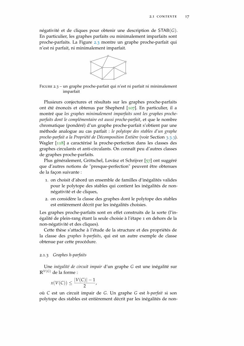
négativité et de cliques pour obtenir une description de STAB(G).En particulier, les graphes parfaits ou minimalement imparfaits sontproche-parfaits. La Figure 2.3 montre un graphe proche-parfait quin’est ni parfait, ni minimalement imparfait.
Figure 2.3 – un graphe proche-parfait qui n’est ni parfait ni minimalementimparfait
Plusieurs conjectures et résultats sur les graphes proche-parfaitsont été énoncés et obtenus par Shepherd [107]. En particulier, il amontré que les graphes minimalement imparfaits sont les graphes proche-parfaits dont le complémentaire est aussi proche-parfait, et que le nombrechromatique (pondéré) d’un graphe proche-parfait s’obtient par uneméthode analogue au cas parfait : le polytope des stables d’un grapheproche-parfait a la Propriété de Décomposition Entière (voir Section 3.3.3).Wagler [118] a caractérisé la proche-perfection dans les classes desgraphes circulants et anti-circulants. On connaît peu d’autres classesde graphes proche-parfaits.
Plus généralement, Grötschel, Lovász et Schrijver [57] ont suggéréque d’autres notions de "presque-perfection" peuvent être obtenuesde la façon suivante :
1. on choisit d’abord un ensemble de familles d’inégalités validespour le polytope des stables qui contient les inégalités de non-négativité et de cliques,
2. on considère la classe des graphes dont le polytope des stablesest entièrement décrit par les inégalités choisies.
Les graphes proche-parfaits sont en effet construits de la sorte (l’in-égalité de plein-rang étant la seule choisie à l’étape 1 en dehors de lanon-négativité et des cliques).
Cette thèse s’attache à l’étude de la structure et des propriétés dela classe des graphes h-parfaits, qui est un autre exemple de classeobtenue par cette procédure.
2.1.3 Graphes h-parfaits
Une inégalité de circuit impair d’un graphe G est une inégalité surRV(G) de la forme :
x(V(C)) ≤ |V(C)| − 12
,
où C est un circuit impair de G. Un graphe G est h-parfait si sonpolytope des stables est entièrement décrit par les inégalités de non-

18 introduction (en français)
négativité, de cliques et de circuits impairs. En d’autres termes, si ona :
STAB(G) =
x ∈ RV(G) :
x ≥ 0,
x(K) ≤ 1 ∀K clique de G,
x(V(C)) ≤ |V(C)| − 12
∀C circuit impair de G.
.
(2.2)
On a déjà noté que les graphes parfaits ne peuvent avoir de trouimpair. Ainsi, le Théorème 2.1.3 montre que les graphes parfaits sonth-parfaits. De plus, le Théorème 2.1.4 implique que les trous impairssont h-parfaits et que les anti-trous impairs à au moins 7 sommets nele sont pas.
L’essentiel des résultats sur la h-perfection porte sur le cas desgraphes qui n’ont pas de clique à 4 sommets. Un graphe est t-parfaits’il est h-parfait et n’a pas de clique de taille 4.
The computational complexity of deciding t-perfection is open.T-perfection belongs to co-NP [102] but no combinatorial certifi-
cate of t-imperfection is available. Neither an NP-characterization oft-perfection nor a co-NP characterization of h-perfection are known.
La complexité algorithmique du problème de la reconnaissanced’un graphe t-parfait est ouverte.
La t-perfection appartient à co-NP [102] mais on ne connaît pas decertificat combinatoire de t-imperfection. Par ailleurs, on ne sait passi la t-perfection appartient à NP ni si la h-perfection est dans co-NP.
Pour tout graphe G et tout poids c ∈ ZV(G)+ , un stable de poids maxi-
mum de (G, c) est un stable S de G pour lequel c(S) est maximum.Grötschel, Lovász, Schrijver ont démontré (par la Méthode des Ellip-soïdes) :
Théorème 2.1.5 (Grötschel, Lovász, Schrijver [56]) Un stable de poidsmaximum d’un graphe h-parfait peut être déterminé en temps polynomial.
Cet résultat donne un exemple d’une propriété majeure de la per-fection qui s’étend à la h-perfection. Eisenbrand et al. [38] ont donnéun algorithme combinatoire efficace pour trouver un stable de cardinalitémaximum dans un graphe t-parfait. Par ailleurs, Bruhn et Stein [16] ontmontré qu’une clique de cardinalité maximum d’un graphe h-parfait peutêtre déterminée efficacement.
Les graphes t-parfaits ont été introduits par Chvátal [26]. Il a conjec-turé que les graphes série-parallèles sont t-parfaits (un graphe estsérie-parallèle s’il n’a pas le graphe complet K4 pour mineur), ce quia été prouvé par Boulala et Uhry [12] (Mahjoub a donné une preuveplus simple dans [77]). Nous terminons cette introduction en dressantl’état des principales connaissances à propos des graphes h-parfaits.

2.1 contexte 19
reconnaissance des graphes h-parfaits Fonlupt et Uhry[44] ont démontré que les graphes presque-bipartis sont t-parfaits (ungraphe est presque-biparti s’il a un sommet qui appartient à tous sescircuits impairs).
Sbihi et Uhry [98] ont prouvé que sous certaines conditions, la sub-stitution de graphes bipartis aux arêtes de graphes série-parallèlesproduit des graphes t-parfaits.
Gerards [50] a étendu les résultats de Fonlupt, Boulala et Uhryen démontrant que les graphes qui n’ont pas de K4-impair (comme sous-graphe) sont t-parfaits (un K4-impair est une subdivision de K4 danslaquelle chaque triangle de K4 est transformé en un circuit impair).
Les subdivisions non-t-parfaites de K4 ont été caractérisées par Ba-rahona et Mahjoub [3]. Gerards et Shepherd [51] ont montré que lesgraphes qui ne contiennent pas de subdivision non-t-parfaite de K4 (commesous-graphe) sont t-parfaits. Ces graphes sont exactement ceux donttous les sous-graphes sont t-parfaits (ils sont dits t-parfaits héréditaires)et peuvent être reconnus en temps polynomial. Ainsi, le résultat deGerards et Shepherd contient tous les précédents énoncés affirmantla t-perfection de graphes ne contenant pas certaines subdivisions deK4, et est maximal quant à l’obtention de t-perfection par exclusionde sous-graphes.
Figure 2.4 – la griffe
Un graphe est sans griffe s’il n’a pas de griffe induite (voir Figure 2.4).Bruhn et Stein [16] ont prouvé une caractérisation combinatoire co-NP de la t-perfection dans les graphes sans griffe. Elle s’exprime entermes de graphes minimalement t-imparfaits relativement à deuxopérations de graphes qui préservent la t-perfection : la suppressiond’un sommet et la t-contraction (celle-ci a été définie et étudiée parGerards et Shepherd [51]).
Bruhn et Schaudt [14] ont utilisé cette caractérisation pour don-ner un algorithme efficace décidant la t-perfection dans la classe desgraphes sans griffe. D’autre part, Shepherd [108] a caractérisé lesgraphes t-parfaits dans la classe des complémentaires de graphes ad-joints.
Les graphes h-parfaits ont été définis par Sbihi et Uhry dans [98].Fonlupt et Hadjar [43] ont montré que sous certaines conditions, lesopérations d’identification de deux sommets et d’ajout d’une arêteconservent la h-perfection. Cao et Nemhauser [19] ont caractérisé lah-perfection dans la classes des graphes adjoints en termes de sous-graphes induits interdits. Un résultat similaire a été obtenu par Arbibet Mosca [2] pour la classe des graphes qui n’ont pas de sous-graphe

20 introduction (en français)
induit isomorphe à un chemin à 5 sommets ou au graphe completauquel on a retiré une arête.
h-perfection forte Des résultats de Lovász [71] et Fulkerson[48] impliquent qu’un graphe est parfait si et seulement si le système desinégalités de non-négativité et de cliques est totalement dual-entier (voir ladéfinition dans la Section 3.3.1).
Les graphes h-parfaits admettent-ils une caractérisation analogue ?Un graphe G est fortement h-parfait si le système des inégalités de
non-négativité, cliques et circuits impairs est totalement dual-entier.Un graphe est fortement t-parfait s’il est fortement h-parfait et sansK4. Des résultats d’Edmonds et Giles [35] impliquent que tout graphefortement t-parfait est t-parfait. Schrijver conjecture la réciproque :
Conjecture (Schrijver [102]) Tout graphe t-parfait est fortement t-parfait.
Il a démontré que les graphes t-parfaits héréditaires sont fortement t-parfaits [101] (on rappelle qu’un graphe est t-parfait héréditaire si tousses sous-graphes sont t-parfaits). Bruhn et Stein [15] ont prouvé queles graphes t-parfaits sans griffe sont fortement t-parfaits.
colorations La caractérisation polyédrale des graphes parfaits(Théorème 1.1.3) montre qu’imposer l’égalité de χ et ω sur tout sous-graphe induit implique que le polytope des stables est entièrementdécrit par les inégalités de non-négativité et de cliques.
Étant donné que les inégalités de circuits impairs sont les seulesintervenant en plus dans la description du polytope des stables d’ungraphe h-parfait, on peut s’attendre à ce que le nombre chromatiqued’un tel graphe reste proche de la taille de sa plus grande clique.
L’existence d’une constante c pour laquelle tout graphe h-parfait Gsatisferait χ(G) ≤ ω(G)+ c n’est pas connue. Laurent et Seymour ontdonné un graphe t-parfait avec χ = 4 et ω = 3 [102, pg. 1207]. Ainsi, cdevrait être supérieure ou égale à 1. Par ailleurs, leur exemple montreque le polytope des stables d’un graphe t-parfait n’a pas la propriétéde décomposition entière [63].
Sebo a prouvé que la (ω + 1)-colorabilité des graphes h-parfaits décou-lerait du cas ω ≤ 2 (voir [16]).
Des résultats de Bruhn et Stein [16] impliquent que tout graphe h-parfait sans griffe est (ω + 1)-colorable (et une coloration optimale peutêtre trouvée en temps polynomial). Enfin, Gerards et Shepherd [51]ont démontré que tout graphe t-parfait héréditaire est 3-colorable (et une3-coloration peut être trouvée efficacement)
Cette thèse se concentre sur l’étude des problèmes de la reconnais-sance des graphes h-parfaits, du calcul de leur nombre chromatiqueet de la propriété de décomposition entière de leur polytope desstables.

2.2 plan de la thèse et contributions 21
2.2 plan de la thèse et contributions
chapitre 3 : préliminaires On donne les notations, défini-tions et résultats nécessaires à la compréhension de la suite du do-cument.
chapitre 4 : sur les opérations qui conservent la h-per-fection Dans ce chapitre, on étudie des opérations de graphesqui préservent la h-perfection et on montre que certaines conserventde plus la propriété de décomposition entière du polytope des stables.
Une t-contraction d’un graphe G est obtenue en identifiant un som-met v à tous ses voisins, lorsque ceux-ci forment un stable de G.Un t-mineur de G est un graphe obtenu à partir de G par une suitede suppressions de sommets et de t-contractions (dans n’importequel ordre). Gerards et Shepherd [51] ont prouvé que les t-mineursconservent la t-perfection.
Nous commençons par étendre ce résultat en démontrant que lest-mineurs conservent aussi la h-perfection. La preuve montre de plus quela perfection est préservée par les t-mineurs.
Un polyèdre P ⊆ Rn a la propriété de décomposition entière si pourtout entier positif k, chaque vecteur entier de kP est la somme de kvecteurs entiers de P.
On prouve aussi que la propriété de décomposition entière du polytopedes stables est conservée par les t-mineurs.
Nous utiliserons ce résultat au Chapitre 7 pour répondre néga-tivement à une question de Shepherd sur les graphes t-parfaits 3-colorables.
Soient G et H des graphes et v un sommet de G. La substitutionde v par H dans G est le graphe obtenu de l’union de deux copiesdisjointes de G− v et H en ajoutant une arête uw pour chaque voisinu de v dans G et chaque sommet w de H. Nous caractérisons lesgraphes qui peuvent être substitués à un sommet d’un graphe h-parfait desorte que le graphe obtenu soit h-parfait lui aussi.
On dit qu’un graphe est minimalement h-imparfait (resp. minimale-ment t-imparfait) s’il est h-imparfait (resp. t-imparfait) et si tout t-mineur de G (sauf G lui-même) est h-parfait (resp. t-parfait).
Comme conséquence de notre résultat sur les substitutions, nousobtenons une propriété des ensembles homogènes dans les graphes mi-nimalement h-imparfaits et t-imparfaits.
chapitre 5 : sur les graphes minimalement h-imparfaits
La t-perfection est une propriété co-NP mais on ne connaît pas decertificat combinatoire de t-imperfection.
L’appartenance de la h-perfection à NP ou co-NP est toujours ou-verte. La caractérisation des graphes minimalement t-imparfaits et

22 introduction (en français)
minimalement h-imparfaits conduirait à une compréhension combi-natoire de ces propriétés.
Nous commencerons par faire l’inventaire des exemples connus degraphes minimalement t-imparfaits. Nous ne donnons pas de nou-vel exemple, mais décrivons leur polytope des stables et formulonsune conjecture à son sujet. De plus, nous énumérons les conjecturesénoncées dans la littérature et en suggérons de nouvelles.
Il est facile de vérifier que K4 est l’unique graphe minimalement t-imparfait qui n’est pas minimalement h-imparfait. On se propose dedéterminer tous les graphes sans K4 qui sont minimalement h-imparfaits etpas minimalement t-imparfaits. Ils montrent que certaines des questionset conjectures formulées pour les graphes minimalement t-imparfaitsne peuvent s’étendre aux minimalement h-imparfaits qu’en excluantcertains cas.
On présente une conjecture de Sebo qui énonce que les graphesminimalement h-imparfaits qui ont des cliques d’au moins 4 sommetssont des antitrous impairs, et nous montrons qu’elle est satisfaite parles graphes planaires. Nous caractérisons aussi les graphes h-parfaits etminimalement h-imparfaits dans la classes des graphes circulants.
Nous expliquons en quoi ces résultats pourraient être utiles dansla recherche d’une preuve de la conjecture de Sebo pour le cas desgraphes sans griffe. Combinée aux résultats de Bruhn et Stein [16],une telle preuve fournirait directement une caractérisation combina-toire co-NP de la h-perfection sans griffe.
Nous observons enfin que les graphes adjoints minimalement h-impar-faits peuvent être facilement obtenus en utilisant un théorème de Caoet Nemhauser [19].
chapitre 6 : propriété d’arrondi entier pour le nombre
chromatique de certains graphes h-parfaits Le nombrechromatique d’un graphe parfait est toujours égal à sa relaxation frac-tionnaire. Ce n’est pas le cas pour les graphes h-parfaits, et on neconnaît pas de borne sur l’écart maximum de ces deux quantités.La détermination de cet écart est liée à la complexité du calcul dunombre chromatique d’un graphe h-parfait. Les résultats principauxde ce chapitre font l’objet de [7].
Pour tout graphe G et tout c ∈ ZV(G)+ , le nombre chromatique (pon-
déré) de (G, c) est le plus petit cardinal d’un multi-ensemble F destables de G tel que tout sommet v de G appartient à au moins cv
membres de F .Nous démontrons que tout graphe h-parfait adjoint et tout graphe t-
parfait sans griffe G a la propriété d’arrondi entier pour le nombre chroma-tique : pour tout poids entier positif c sur les sommets, le nombrechromatique de (G, c) s’obtient en arrondissant sa relaxation fraction-naire à l’entier supérieur. En d’autres termes, le polytope des stables deG a la propriété de décomposition entière.

2.2 plan de la thèse et contributions 23
Ces résultats impliquent l’existence d’un algorithme polynomialpour le calcul du nombre chromatique pondéré d’un graphe t-parfait sansgriffe ou h-parfait adjoint. Par ailleurs, ils fournissent un nouveau casd’une conjecture de Goldberg et Seymour [55, 104] sur l’arête-coloration.
Sebo [103] a prouvé que toute projection d’un polyèdre défini pardes contraintes totalement unimodulaires à la propriété de décompo-sition entière. Nous terminons ce chapitre en montrant que la réci-proque est fausse, même pour les polytopes 0-1.
chapitre 7 : sur la coloration des graphes h-parfaits
En utilisant le fait que les t-mineurs conservent la propriété de dé-composition entière du polytope des stables (prouvé au Chapitre 3),nous résolvons un problème de Shepherd [108] sur les graphes t-parfaits3-colorables.
D’autre part, nous prouvons une caractérisation (par exclusion desous-graphes induits) de la propriété d’arrondi entier du nombre chro-matique pour les poids 0-1 dans les graphes h-parfaits complémentaires degraphes adjoints. Un des deux sous-graphes interdits est un nouvelexemple de graphe t-parfait qui n’est pas 3-colorable.
Un graphe est sans P6 s’il n’a pas de sous-graphe induit isomorpheau chemin à 6 sommets. Après un inventaire des résultats et conjec-tures sur le nombre chromatique des graphes h-parfaits, nous mon-trons qu’un résultat de Randerath, Schiermeyer et Tewes [93, 94] im-plique que tout graphe h-parfait sans P6 est (ω+ 1)-colorable. Cette borneest serrée et une (ω + 1)-coloration peut être trouvée en temps poly-nomial.
chapitre 8 : décomposition d’oreilles et h-perfection
dans les graphes adjoints La complexité de la reconnaissancedes graphes h-parfaits est ouverte. Dans ce chapitre nous étudions lecas des graphes adjoints, pour lesquels le problème a une formulationcombinatoire simple. Notre solution met en évidence des liens entreles espaces binaires, l’arête-coloration, certaines subdivisions de K4 etles décomposition d’oreilles. Les résultats de ce chapitre font l’objetde [8].
Notons C+3 le graphe obtenu du triangle en ajoutant une seule arête
parallèle. Un C+3 -impair est un graphe obtenu en remplaçant chaque
arête e de C+3 par une chaîne ayant un nombre impair d’arêtes, de
sorte que les chaînes correspondant à des arêtes différentes ne par-tagent pas de sommets internes deux-à-deux. Un graphe est dit sansC+
3 -impair s’il n’a pas de sous-graphe isomorphe à un C+3 -impair.
Des résultats de Kawarabayashi, Reed, Wollan [66] (et Huynh [62])impliquent qu’il est possible de détecter un C+
3 -impair (comme sous-graphe) en temps polynomial. De plus, Bruhn et Schaudt [14] ontdonné un algorithme efficace plus simple pour le cas des graphes dedegré maximum 3.

24 introduction (en français)
Nous proposons un algorithme simple et élémentaire pour la reconnais-sance des graphes sans C+
3 -impair (sans restriction sur les degrés). Il peutêtre converti en un algorithme efficace qui décide la h-perfection dans lesgraphes adjoints.
Soit G un graphe. On note β(G) le plus grand entier k tel que G aun sous-graphe qui admet une décomposition d’oreilles ouverte aveck oreilles (voir Section 3.2.2 pour la définition de ces termes). Parexemple, β(G) ≤ 1 si et seulement si G est sans C+
3 -impair.Nous prouvons que le calcul de β est résoluble en temps polynomial à
paramètre fixé et énonçons une conjecture sur la propriété d’arrondientier de l’indice chromatique des graphes pour lesquels β est petit.
D’autre part, nous donnons un algorithme efficace simple pour la dé-tection de subdivisions totalement impaires de K4 dans les graphes sans C+
3 -impair.
La relation des graphes sans C+3 -impair aux subdivisions totale-
ment impaires de K4 a été mise en évidence dans la thèse de Cao [18].Cette dernière contient des résultats structurels et des constructionspour les graphes simples sans C+
3 -impair. Nous clôturons le chapitreavec l’énumération des principaux résultats de [18] liés aux graphessans C+
3 -impair et observons que certains énoncés sont incorrects.
chapitre 10 : conclusion On résume les questions et conjec-tures énoncées dans les chapitres précédents. On suggère enfin di-verses perspectives de recherche pour la poursuite de l’étude de lah-perfection et des problèmes liés.

3P R E L I M I N A R I E S
This chapter contains the notations, definitions and results which are nec-essary in understanding the rest of the document. No new result is givenand it is intended as a reference chapter only.
With a few exceptions, we do not provide proofs. Indeed, the content isstandard regarding the combinatorial optimization literature and they canbe found in the indicated references.
Ce chapitre contient l’ensemble des notations, définitions et résultats né-cessaires à la compréhension de la suite de la thèse. Il ne propose pas denouveau résultat et est conçu en tant que référence pour les chapitres sui-vants.
Les résultats énoncés sont pour la plupart standards en OptimisationCombinatoire. À quelques exceptions près nous ne fournissons pas leurspreuves et proposons des références qui les contiennent.
3.1 numbers , sets and families
The sets of integers, rational numbers and real numbers are respec-tively denoted Z, Q, R. The set of non-negative integers is writtenZ+ and the set of non-negative rational numbers is denoted Q+. Wewrite ∅ for the empty set. For every real number x, let bxc (resp. dxe)denote the floor (resp. ceiling) of x.
We will use the usual convention: max∅ = +∞ and min∅ = −∞.For each non-negative integer k, we put [k] := {1, . . . , k}. Finally, wewrite F2 for the field with 2 elements. The all-1 vector of a finite-dimensional vector space is always written 1 without further preci-sion (there shall not be any ambiguity).
Let S be a set. The number of elements (or cardinality) of S is writ-ten |S|. The incidence vector of a subset Y of S, denoted χY, is the vectorof RS defined for every s ∈ S by: χY(s) = 1 if s ∈ Y and χY(s) = 0otherwise. If Y has a single element s, we write χs instead of χ{s}. Forevery x ∈ RS, let x(Y) denote ∑s∈Y xs.
For each Y ⊆ S, we define the projection of RS on RY as the mapπ : RS → RY which sends each vector x ∈ RS to its restriction to Y.That is, the map just deletes the coordinates indexed by the elementsof S \ Y. We often refer to π simply as the projection RS → RY. Theprojection of X ⊆ RS on RY is the set π(X).
For elements u, v of a set X, we write uv for the set {u, v}. A pair isa set of cardinality 2. The symmetric difference of two sets X and Yis denoted X∆Y.
25

26 preliminaries
A multiset is a set in which the same element can occur more thanonce. The number of occurrences of an element is its multiplicity.
The cardinality of a multiset F , denoted |F | (extending the notationfor sets), is the sum of the multiplicities of the elements of F .
The sum of two multisets F1 and F2, denoted F1 +F2, correspondsto their union in which multiplicities are added. If F2 consists of a sin-gle element s with multiplicity 1, we write the sum F1 + s instead ofF1 + {s}. The difference F1 − F2 of F1 and F2 is obtained by remov-ing from F1 each element s of F2 as many times as its multiplicityin F2 (if the latter is greater than the multiplicity in F1, then we sim-ply delete every occurrence of x from F1). Similarly, we write F1 − xinstead of F1 − {x}.
A subset (resp. submultiset) of a set S (resp. multiset) is proper ifit is different from S. An element of a set F of subsets of a set X isinclusion-wise maximal if it is not a proper subset of an element of F .Besides, F covers X if each element belongs to at least one memberof F . It is easy to check that if F is closed by taking subsets, then Fcovers X if and only if X can be partitioned into members of F .
The symbol � marks the end of the proof of a proposition, lemma,theorem, corollary, whereas � denotes the end of a proof of a claiminside a larger proof.
For further standard and basic related notations and notions, werefer to Chapter 2 of [102].
3.2 graphs
In this thesis we only consider finite undirected graphs. They canhave multiple edges but no loops.
Let G be a graph. The set of vertices and the set of edges of G arerespectively denoted V(G) and E(G). The ends of an edge e of G areits two elements. We use the notation e = uv to specify that u and vare the ends of e. Two vertices u and v of G are adjacent if G has anedge whose ends are u and v.
Edges are parallel if they have the same ends. The multiplicity of anedge e of G is the number of edges which are parallel to e (includinge). Besides, G is simple if its edges all have multiplicity 1.
A graph is complete if its vertices are pairwise-adjacent. For eachX ⊆ V(G), the set of edges which have both ends in X is writtenEG(X).
Let v be a vertex of G. A neighbor of v in G is a vertex adjacent to u.The neighborhood of v in G, denoted NG(v), is the set of neighbors ofv in G. Besides, let NG [v] := NG(v) ∪ {v}.
An edge e and a vertex u of G are incident if u is an end of e. Twoedges are incident if they have at least one common end.

3.2 graphs 27
3.2.1 Basic notions
degrees For each vertex u of G, we write δG(u) for the set ofedges of G which are incident with u. The degree of u in G, denoteddG(u), is the number |δG(u)|. The largest degree of a vertex of G iswritten ∆(G). A vertex of G is isolated if it has degree 0 (that is ithas no neighbor). Unless G is simple, the degree and the number ofneighbors of a vertex may differ.
A graph is k-regular if its vertices all have the same degree k. In thiscase, we say that k is the degree of the graph.
Figure 3.1 – a 3-regular simple graph (Petersens’s graph)
isomorphisms Two graphs G1 and G2 are isomorphic if there existbijective maps f : V(G1) → V(G2) and g : E(G1) → E(G2) such thatfor each uv ∈ E(G1), the ends of g(uv) are f (u) and f (v).
If G1 and G2 are simple, then this is equivalent to state that thereexists a bijective map (called an isomorphism) f : V(G1)→ V(G2) suchthat for every pair uv of vertices of G1: the pair f (u) f (v) is an edgeof G2 if and only if uv is an edge of G1.
A simple graph H is vertex-transitive if for each pair of vertices uand v of G, there exists an isomorphism of G onto itself which sendsu to v.
a1
a2
a3 a4
b1 b2
b3 b4
Figure 3.2 – two isomorphic graphs (ai → bi is an isomorphism)
operations on graphs For each F ⊆ E(G), let G − F denotethe graph (V(G), E(G)− F). We say that G− F is obtained from G bydeleting F and we refer to this operation as an edge-deletion. If F has asingle element e, then we write G− e instead of G− {e}.

28 preliminaries
The underlying simple graph of G is the graph (unique up to isomor-phism) obtained from G by deleting edges until no pair of paralleledges remains.
For each set F of pairs of vertices of G, let G + F denote the graph(V(G), E(G) + F). We say that G + F is obtained from G by addingthe pairs of F as edges. If F has a single element e, then we write G + einstead of G + {e}.
For each X ⊆ V(G), let G − X denote the graph obtained from Gby deleting each vertex of X and each edge of G incident to a vertexof X. We say that G−X is obtained from G by deleting X and we referto this operation as a vertex-deletion. If X has a single element v, thenwe write G− v instead of G− {v}.
Let x be a new element which does not belong to V(G) and let Fbe the set of edges of G which have no end in X. We define:
E := F + {ux : ∀uv ∈ E(G) with v ∈ X and u /∈ X} .
The pair (V(G)− X + x, E) is a graph, denoted G/X and we say thatit is obtained from G by identifying (or shrinking) the vertices of X to asingle vertex (see Figure 3.3).
X(a) G
x(b) G/X
Figure 3.3 – shrinking a set X of vertices of G to a single vertex x
For each edge e = uv of G, we write G/e for G/ {u, v} and say thatG/e is obtained from G by contracting e. We refer to this operationas an edge-contraction. A minor of G is a graph obtained from G by asequence of vertex or edge-deletions and edge-contractions.
subgraphs A graph H is a subgraph of G if V(H) ⊆ V(G) andE(H) ⊆ E(G). It is proper if it is distinct from G, and it is spanningif V(H) = V(G). For each graph H, we will say that G contains H ifG has a subgraph isomorphic to H. For each X ⊆ V(G), the subgraphof G induced by X, denoted G [X], is the subgraph G− (V(G) \ X). Inother words, it is the graph (X, EG(X)). A subgraph H of G is inducedif it is induced by some subset of vertices of G.
For each simple graph H, we say that G contains an induced H (orthat G has an induced H) if G has an induced subgraph whose un-derlying simple graph is isomorphic to H.

3.2 graphs 29
If G is simple, then G has an induced H if and only if there existsX ⊆ V(G) such that H = G [X].
Two subgraphs are vertex-disjoint (resp. edge-disjoint) if they do nothave a common vertex (resp. edge).
union. intersection. complement The union of G1 and G2,denoted G1 ∪ G2, is the graph (V(G1) ∪V(G2), E(G1) ∪ E(G2)). Theirintersection, denoted G1 ∩ G2, is the graph (V(G1) ∩ V(G2), E(G1) ∩E(G2)).
The complement of a graph G, denoted G, is the simple graph whosevertex-set is V(G) and whose edges are the pairs of non-adjacentvertices of G.
paths , circuits and connectivity A path P of G is a se-quence (u1, . . . , uk) (with k ≥ 1) of pairwise-distinct vertices of Gsuch that for each i ∈ [k− 1]: uiui+1 ∈ E(G). We will often identify itto the subgraph ({u1, . . . , uk} , {u1u2, . . . , uk−1uk}).
The vertices u1 and uk (which may be the same) are the ends ofP and u2, . . . , uk−1 are the inner vertices of P. Besides, we say that Pjoins its ends. Two paths are inner-disjoint if they do not share innervertices. For u, v ∈ V(G), a uv-path of G is a path joining u to v.
Let v ∈ V(G). The component of v in G is the subgraph of G inducedby the set of vertices which are joined to v by a path in G. The compo-nents of the vertices of G define a partition of its vertex-set. A graphis connected if it is a component of itself.
A circuit is a 2-regular connected graph. A circuit of G is a subgraphof G which is a circuit.
The length of a path (or circuit) is the number of its edges. A k-circuit is a circuit of length k. A path (or circuit) is odd if it has oddlength, and even otherwise. For u, v ∈ V(G), the distance of u and v inG, denoted dG(u, v), is the smallest length of a uv-path of G.
A chord of a circuit C of G is an edge of G whose ends are twonon-adjacent vertices of C.
A hole of G is a circuit of G which has length at least 4 and no chord.An antihole of G is a subgraph of G which is the complement of a holeof G.
A hole (or antihole) is odd if it has an odd number of vertices.
trees A graph is a tree if it is connected and does not contain acircuit. It is well-known that each connected graph has a spanning tree.Besides, an easy induction shows that each tree with n vertices has n− 1edges. Therefore, each spanning tree of a connected graph G has |V(G)| − 1edges.
subdivisions A graph H is a subdivision of G if it is obtained fromG by replacing each edge e ∈ E(G) with a path Pe (of non-zero length)

30 preliminaries
joining the ends of e such that: for every pair of edges e, f ∈ E(G),the paths Pe and Pf do not share inner vertices.
If each odd circuit of G stays odd in the subdivision, we say that His an odd subdivision of G. If each Pe has odd length, then we further-more say that H is a totally odd subdivision of G (see Figure 3.4).
Figure 3.4 – non-totally and totally odd subdivisions of K4
line graph The line graph of G, denoted L(G), is the simple graphwhose vertices are the edges of G and whose edge-set is the set ofpairs of incident edges of G. A graph H is a line-graph if there existsa graph G such that H = L(G).
graphs Kn , Pn , Cn Simple complete graphs (or paths, circuits)of the same size are obviously isomorphic to each other. We givenotations to represent each of these isomorphism classes.
Let n ≥ 1 be an integer and Vn := {v1 , . . . , vn} be a set of nelements.
The graph Kn is the complete graph whose vertex-set is Vn (seeFigure 3.5). A graph is Kn-free if it does not contain Kn .
K3 K4 K5
Figure 3.5 – examples of complete graphs
Let Pn denote the graph whose vertex-set is Vn and whose edge-set is E(Pn ) := {v1 v2 , . . . , vn−1 vn}. A graph is Pn-free if it does nothave an induced Pn .
Finally, for n ≥ 2 the graph Cn is defined by V (Cn ) := Vn andE(Cn ) := E(Pn ) ∪ {v1 vn} (see Figure 3.6).
wheels Let n ≥ 3 be an integer. Let Wn denote the graph ob-tained from Cn by adding a new vertex cn (the center of Wn) and

3.2 graphs 31
C3 C4 C5
P5
Figure 3.6 – examples of circuits and paths
every edge between Cn and cn . The graph Wn is the wheel of size n (orn-wheel)(see Figure 3.7). The circuit Cn of Wn is the rim of Wn .
W3 W4 W5
Figure 3.7 – examples of wheels
webs and antiwebs Let k ≥ 1 and n ≥ 3 be integers. Let Ek bethe set of pairs uv of vertices of Cn such that dCn(u, v) ≤ k. The graphCk
n is defined as Cn + Ek. For example, if n ≤ 2k + 1 then Ckn = Kn.
Besides, Cn = C1n.
A graph is a web if it is isomorphic to a Ckn. An antiweb is the com-
plement of a web.
C27 = C7 C2
10
Figure 3.8 – examples of webs

32 preliminaries
3.2.2 Higher connectivity. Menger’s theorem. Ear-decompositions
disjoint paths We will use Menger’s theorem several times inthis thesis. We follow the exposition of Chapter 9.1 in [102].
Let G be a graph and S, T be subsets of V(G). An {S, T}-path is apath joining a vertex of S to a vertex of T. An {S, T}-separator of G isa subset of vertices of G meeting every {S, T}-path.
Theorem 3.2.1 (Menger [80]) Let G be a graph and S, T ⊆ V(G). Themaximum number of vertex-disjoint {S, T}-paths is the minimum cardinal-ity of an {S, T}-separator of G.
A maximum number of vertex-disjoint {S, T}-paths can be foundin polynomial-time (by a reduction to the max-flow min-cut algo-rithm of Ford and Fulkerson [45, 46]. When max(|S|, |T|) ≤ 2, therecent and faster algorithm of Tholey [114] can also be used.
cuts and connectivity Let G be a graph. A vertex-cut of G is aset X ⊆ V(G) whose deletion increases the number of components ofG. A vertex-cut having k elements is called a k-vertex-cut. The uniqueelement of a 1-cut is a cut-vertex of G.
For each positive integer k, a graph is k-connected if it has morethan k vertices and no k-cut. A graph is k-edge-connected if deletingless than k edges cannot increase the number of components.
blocks A bridge of a graph is an edge whose deletion increasesthe number of components. A block of a graph G is either an isolatedvertex or the subgraph induced by the two ends of a bridge or a 2-connected subgraph of G which is maximal for the subgraph relation.
Two blocks cannot intersect on more than one vertex, which mustbe a cut-vertex.
ear-decompositions An ear-decomposition of a graph G is a se-quence (C, P1, . . . , Pk) of a circuit C and paths (or circuits) P1, . . . , Pk ofG (with k ≥ 0) such that G = C∪ P1 ∪ · · · ∪ Pk and for each i ∈ [k]: if Piis a path, then exactly its ends are vertices of C∪ (P1 ∪ · · · ∪ Pi−1) andif Pi is a circuit, then Pi has exactly one vertex in C ∪ (P1 ∪ · · · ∪ Pi−1).The paths or circuits C, P1, . . . , Pk are the ears of the decomposition.
The decomposition is open if P1, . . . , Pk are all paths and C haslength at least 3. Besides, it is odd if all the ears have odd length.
Theorem 3.2.2 (Whitney [120]) A graph has an open ear-decompositionif and only if it is 2-connected.
Theorem 3.2.3 (Robbins [95]) A graph has an ear-decomposition if andonly if it is 2-edge-connected.
The following shows that all ear-decompositions of a 2-edge-connectedgraph have the same number of ears:

3.2 graphs 33
Proposition 3.2.4 Let G be a 2-edge-connected graph.The ear-decompositions of G have the same number of ears, which is:
|E(G)| − |V(G)|+ 1.
Proof – Let (C, P1, . . . , Pk) be an ear-decomposition of G.Let e ∈ E(C) and for each 1 ≤ i ≤ k, let ei ∈ E(Pi). It is easy to
check that T := G − e− e1 − · · · − ek is a spanning tree of G. Hence,the number of edges of G which do not belong to T is k + 1. Since Tis a tree: |E(T)| = |V(G)| − 1.
Therefore, k = |E(G)| − |V(G)|+ 1.
�Hence, we may speak of the number of ears of a 2-edge-connected
graph. This number is also known as the cyclomatic number of thegraph.
Using Menger’s theorem (Theorem 3.2.1), it is straightforward tocheck the following:
Proposition 3.2.5 Let G be a 2-edge-connected graph.Each ear-decomposition of a 2-edge-connected subgraph H of G can be
completed in an ear-decomposition of G.Furthermore if G is 2-connected, then the ear-decomposition of H can be
completed with open ears.
3.2.3 Cliques, stable sets, matchings.
Let G be a graph. A subset of vertices of G is a clique if it inducesa complete subgraph of G. In other words, it is a set of pairwise-adjacent vertices of G. A triangle is a clique of 3 vertices.
A stable set of G is a set of pairwise-non-adjacent vertices of G. Thatis a clique of G.
A matching of G is a set of pairwise-non-adjacent edges of G, thatis a stable set of L(G). A matching is perfect if it covers every vertexof G.
Let c ∈ ZV(G)+ . The stability number of (G, c), denoted α(G, c), is the
largest value of c(S) over all stable sets S of G. Similarly, the cliquenumber of (G, c), denoted ω(G, c), is defined by ω(G, c) := α(G, c). Itis the largest value of c(K) over all cliques K of G.
A stable set (resp. clique) of G is of maximum-weight in (G, c) if itattains the value α(G, c) (resp. ω(G, c)). We say that a stable set (orclique) of G is maximum if it has maximum cardinality in G.
Let d ∈ ZE(G)+ . The matching number of (G, d), denoted ν(G, d), is
the maximum of d(M) over all matchings M of G. In other words,ν(G, d) = α(L(G), d).
In particular, the stability number, clique number and matching num-ber of G are defined respectively as α(G) := α(G, 1), ω(G) := ω(G, 1)and ν(G) := ν(G, 1). That is, they are respectively the largest cardi-nalities of a stable set, clique or matching of G.

34 preliminaries
3.2.4 Graph colorings
chromatic number Let G be a graph and k be a non-negativeinteger. A k-coloring of G is a map from V(G) → [k] which assignsdistinct numbers (called colors) to adjacent vertices. We say that G isk-colorable if it admits a k-coloring. Clearly, G is k-colorable if and onlyif V(G) can be covered by (equivalently, partitioned into) k stable sets.
The chromatic number of G, denoted χ(G), is the smallest integersuch that G is k-colorable.
bipartite graphs A graph is bipartite if it is 2-colorable. That is,it has a bipartition: a partition of its vertex-set into two stable sets. Itis easy to show that a graph is bipartite if and only if it does not containan odd circuit.
clique-cover number The clique-cover number of G is denotedχ(G) and is defined as χ(G) := χ(G). In other words, it is the smallestnumber of cliques needed to cover (equivalently, partition) the vertex-set of G.
chromatic index A k-edge-coloring of G is a map from E(G) →[k] which assigns distinct numbers to incident edges: it is a k-coloringof L(G). We say that G is k-edge-colorable if it has a k-edge-coloring.Hence, G is k-edge-colorable if and only if its edge-set can be covered(or partitioned) with k matchings.
The chromatic index of G, denoted χ′(G), is the smallest integer ksuch that G is k-edge-colorable. Equivalently, χ′(G) = χ(L(G)).
weighted colorings Let c ∈ ZV(G)+ and k be a positive integer.
A k-coloring of (G, c) is a multiset F of cardinality k formed by stablesets of G such that each v ∈ V(G) belongs to at least cv members of F .We say that (G, c) is k-colorable if it admits a k-coloring. The chromaticnumber of (G, c), denoted χ(G, c), is the smallest integer k such that(G, c) is k-colorable.
Let S(G) denote the set of stable sets of G. It is easy to check thatwe have:
χ(G, c) = min
{∑
S∈S(G)
yS : y ∈ ZS(G)+ ; ∑
S∈S(G) : v∈SyS ≥ cv, ∀v ∈ V(G)
}.
(3.1)
Clearly, χ(G, 1) = χ(G). The clique-cover number of (G, c), denotedχ(G, c), is defined by χ(G, c) := χ(G, c) and we have χ(G, 1) = χ(G).
In general, we will often speak of a coloring (or clique-cover) with-out referring to its cardinality. A coloring (resp. clique-cover) of (G, c)is optimal if it uses χ(G, c) stable sets (resp. χ(G, c) cliques).

3.3 linear programming and polyhedra 35
3.3 linear programming and polyhedra
We refer to Chapter 7 and 8 of [100] for the proofs of the resultsstated in this section.
3.3.1 Linear programming
matrices and inequalities Vectors are column-matrices bydefault and matrices are always of finite size. For each matrix M, wewrite MT for the transpose of M. We use only the standard productof matrices. A matrix of is rational if its coefficients are all rationalnumbers. It is furthermore integral if its coefficients are all integers.For a positive integer k, we say that a rational matrix M is 1
k -integralif kM is integral.
A linear inequality over Rn is an inequality of the form aTx ≤ b(x ∈ Rn), where a ∈ Rn and b ∈ R. Such an inequality is rational if aand b are rational. It is tight for y ∈ Rn if aTy = b.
In this thesis, we only consider systems of finite number of rationalinequalities.
the duality theorem Several times throughout this document,we will use the duality theorem of linear programming (due to VonNeumann [117]) in the following form. We refer to Chapter 7 in [100]for further details on this theorem and the complementary slacknesscorollary.
Theorem 3.3.1 (Duality theorem of linear programming) For every ra-tional matrix A with m rows and n columns and each c ∈ Qn and b ∈ Qm:
max cTx = min min yTb
s.t Ax ≤ b yTA ≥ cT
x ≥ 0 y ≥ 0
(3.2)
If the maximum is finite, then both the maximum and the minimum areattained by rational vectors.
We will also use the following corollary:
Corollary 3.3.2 (Completementary slackness) In Theorem 3.3.1, ifthe maximum is finite then: for every pair of respective optimal solutions xand y for the maximum and the minimum, we have yT(Ax− b) = 0.
total dual-integrality Let A be a rational matrix with mrows and n columns and b ∈ Qm. The system of linear inequalities{Ax ≤ b, x ≥ 0} over Rn is totally dual-integral if for every c ∈ Zn
such that:
min{
yTb : yTA ≥ cT; y ≥ 0}

36 preliminaries
is finite, this minimum is attained by an integral vector.We use this notion through the following result due to Edmonds
and Giles:
Theorem 3.3.3 (Edmonds, Giles [35]) If {Ax ≤ b, x ≥ 0} is a total dual-integral system over Rn and if b is integral then, for every c ∈ Zn such that:
max{
cTx : Ax ≤ b, x ≥ 0}
is finite, this maximum is attained on an integral vector.
3.3.2 Affine spaces and maps
A set A is an affine subspace of Rn it is of the form A = u + F,where u ∈ Rn and F is a linear subspace of Rn. The linear space F isuniquely determined by A and is called the direction of A.
An affine combination of a finite number of vectors x1, . . . , xk of Rn
is a vector of the form ∑ki=1 λixi, where λ1, . . . , λk are real numbers
satisfying ∑ki=1 λi = 1. The vectors x1, . . . , xk are affinely independent if
for every (λ1, . . . , λk) ∈ Rk such that ∑ki=1 λixi = 0 and ∑k
i=1 λi = 0,we have λ1 = · · · = λk = 0. Linear independent vectors are obviouslyaffinely independent too.
Let X ⊆ Rn. The set of all affine combinations of the elements ofX is an affine subspace of Rn. It is the affine hull of X and is denotedaff(X).
The dimension of an affine subspace A of Rn is the dimension of itsdirection (as a linear subspace). It is easy to check that is is the largestnumber of affinely independent vectors of A minus one. The dimension of asubset X of Rn is the dimension of aff(X).
3.3.3 Polyhedra
A set P ⊆ Rn is a polyhedron if there exists a finite number of linearinequalities aT1 x ≤ b1, . . . , aTk x ≤ bk (x ∈ Rn) such that:
P ={
x ∈ Rn : aTi x ≤ bi ∀i ∈ [k]}
.
Such a set of inequalities is a description of P. We also say that P isdescribed by these inequalities. Besides, P is rational if the inequalitiesaT1 x ≤ b1, . . . , aTk x ≤ bk are rational.
A polyhedron of Rn is full-dimensional if it has dimension n. Thatis, P contains n + 1 affinely independent vectors.
In this thesis, we only consider rational polyhedra and almost al-ways deal with full-dimensional ones.
faces A linear inequality aTx ≤ b over Rn is valid for P if everyx ∈ P satisfies aTx ≤ b.

3.3 linear programming and polyhedra 37
A non-empty set F ⊆ P is a face of P if there exists a valid inequalityaTx ≤ b for P such that F =
{x ∈ P : aTx = b
}. We say that the in-
equality aTx ≤ b defines F. It is straightforward to check that the facesof P are polyhedra themselves and that a non-empty intersection offaces is also a face.
integrality P is integral if each face of P contains an integralpoint. Since the set of optimal solutions of a linear program is clearlya face of the underlying polyhedron, we have the following straight-forward characterization:
Proposition 3.3.4 Let P ⊆ Rn be a polyhedron. The following statementsare equivalent:
i) P is integral,ii) for every c ∈ Zn such that max
x∈PcTx is finite, this maximum is at-
tained by an integral point.
facets A facet of a polyhedron P is an inclusion-wise maximalproper face of P. The following characterization can be obtained as aconsequence of the duality theorem of linear programming and basiclinear algebra arguments:
Proposition 3.3.5 Let P ⊆ Rn be a full-dimensional polyhedron and F bea face of P. The following statements are equivalent:
i) F is a facet of P,ii) F contains n affinely independent vectors.
This directly implies that for each facet F of a full-dimensional poly-hedron P, the valid inequalities for P which define F are positivemultiples of each other. That is, F is defined by a unique valid inequality(up to a positive scalar factor).
Let P be a polyhedron and S be a set of inequalities describing P.An inequality e ∈ S is redundant if S− e also describes P. A descrip-tion of P is irredundant if its has no redundant inequality. The follow-ing result links inequalities of irredundant descriptions and facets:
Proposition 3.3.6 For every full-dimensional polyhedron P ⊆ Rn andeach irredundant description aT1 x ≤ b1, . . . , aTk x ≤ bk of P, the followingstatements hold:
i) Each inequality aTi x ≤ bi (i ∈ [k]) defines a facet of P,ii) Each facet of P is defined by a unique inequality aTi x ≤ bi (i ∈ [k]).
vertices Let P be a polyhedron. A vertex of P is a u ∈ P such thatfor every v, w ∈ P: u = v+w
2 implies u = v = w. Equivalently, {u}is a face of P. We will frequently use the following characterization ofvertices of a polyhedron:

38 preliminaries
Proposition 3.3.7 Let P ⊆ Rn be a polyhedron described by the inequal-ities aT1 x ≤ b1, . . . , aTk x ≤ bk and let u ∈ P. The following statements areequivalent:
i) u is a vertex of P,ii) there exist n inequalities aTi1 x ≤ bi1 , . . . , aTin
x ≤ bin which are tightfor u and such that the vectors ai1 , . . . , aik are linearly independent (orspan Rn).
It is easy to check that if P is an integral polyhedron contained in [0, 1]n,then each integral point of P is a vertex of P.
polytopes A convex combination of vectors a1, . . . , ak of Rn is avector of the form ∑k
i=1 λiai, where λ1, . . . , λk are real non-negativenumbers such that ∑k
i=1 λi = 1. The convex hull of a set X ⊆ Rn is theset of all convex combinations of elements of X.
A polytope of Rn is the convex hull of a finite set X ⊆ Rn. The finitebasis theorem for polytopes (attributed to Minkowski [82], Steinitz[110] and Weyl [119]) states that:
Theorem 3.3.8 (Finite basis theorem for polytopes) A set P ⊆ Rn
is a polytope if and only if it is a bounded polyhedron.
Hence, the terminology given for polyhedra also applies to poly-topes. In particular, it is straightforward to check that a polytope is theconvex hull of its vertices. This implies easily that a polytope is integral ifand only if its vertices are integral.
integer decomposition property For each subset X ⊆ Rn
and each λ ∈ R, let λX := {λx : x ∈ X}.A polyhedron P ⊆ Rn has the integer decomposition property (abbre-
viated IDP) if for every positive integer k, each integral vector of kPis the sum of k integral vectors of P.
3.4 the stable set polytope
3.4.1 Definitions. General properties
stable set polytope Let G be a graph. The stable set polytope ofG, denoted STAB(G), is the convex hull of the incidence vectors ofthe stable sets of G. In particular, for every c ∈ Z
V(G)+ :
α(G, c) = max{
cTx : x ∈ STAB(G)}
.
Clearly, STAB(G) is a full-dimensional polytope. Hence, Proposi-tion 3.3.6 shows that STAB(G) can be uniquely described as the setof solutions of a system of linear inequalities (up to positive scalar

3.4 the stable set polytope 39
multiplication of these). It is not possible to test in polynomial-time if agiven vector belongs to STAB(G), unless P = NP (see [64]).
It is easy to check that for each v ∈ V(G), the inequality xv ≥ 0defines a facet of STAB(G). They are the non-negativity inequalities anddefine the trivial facets of STAB(G).
fractional colorings Let S(G) denote the set of stable sets ofG and let c ∈ Z
V(G)+ . The fractional chromatic number of (G, c), denoted
χ f (G, c), is defined as the optimum value of the linear relaxation ofthe integer program (3.1) for χ(G, c):
χ f (G, c) := min
{∑
S∈S(G)
yS : y ∈ RS(G)+ ; ∑
S∈S(G) : v∈SyS ≥ cv, ∀v ∈ V(G)
}.
(3.3)
In particular, we always have χ(G, c) ≥ χ f (G, c). A fractional coloringof (G, c) is a feasible solution for the minimum above. Theorem 3.3.1implies directly that (G, c) always has a rational optimal fractional color-ing.
The fractional chromatic number of G, denoted χ f (G), is defined byχ f (G) := χ f (G, 1).
Clearly, an inequality aTx ≤ b defining a non-trivial facet of STAB(G)
must satisfy a ≥ 0 and b > 0. The duality theorem of linear program-ming implies the following:
Proposition 3.4.1 Let G be a graph and c ∈ ZV(G)+ .
If STAB(G) is completely described by non-negativity inequalities andaT1 x ≤ b1, . . . , aTk x ≤ bk (where a1, . . . , ak are non-negative and b1, . . . , bkare positive), then:
χ f (G, c) = maxi∈[k]
cTai
bi. (3.4)
Proof – Let M := maxi∈[k]
cTai
bi. By the duality theorem of linear pro-
graming (Theorem 3.3.1), we have:
χ f (G, c) = max{
cTx : x ≥ 0; x(S) ≤ 1 for all S ∈ S(G)}
. (3.5)
Clearly, aibi
belongs to the polytope defined by the inequalities x ≥ 0and x(S) ≤ 1 (for all S ∈ S(G)). This shows that χ f (G, c) ≥ M.
Let d ∈ RV(G) attaining the maximum in Equation (3.5). By theduality theorem of linear programming:
max{
dTx : x ∈ STAB(G)}= min
{k
∑i=1
yibi : y ≥ 0;k
∑i=1
yiaTi ≥ dT}
.

40 preliminaries
Let y be a vector attaining the minimum in this equation. Since the in-equality dTx ≤ 1 is valid for STAB(G), we have ∑k
i=1 yibi ≤ 1. Hence:
χ f (G, c) = cTd ≤k
∑i=1
yibicTai
bi≤ (
k
∑i=1
yibi)M ≤ M,
as required.
�
computing χ f The maximum-weight stable set problem is as follows:
for a graph G and a weight c ∈ ZV (G)+ , find a stable set S of G such
that c(S) is maximum. This problem is NP-hard in general [64].The problem of the computation of the (weighted) fractional chro-
matic number of a graph and the maximum-weight stable set prob-lem are related as follows (through the Ellipsoid method):
Theorem 3.4.2 (Grötschel, Lovász and Schrijver [57]) Let C be a classof graphs. The following statements are equivalent:
i) the fractional chromatic number of (G , c) can be computed in polyno-mial time for every G ∈ C and every c ∈ Z
V (G)+ ,
ii) the maximum-weight stable set problem can be solved in polynomialtime in C .
integer decomposition property Results of Baum and Trot-ter imply the following characterization for the integer decompositionproperty of the stable set polytope:
Theorem 3.4.3 (Baum, Trotter[4]) Let G be a graph. The following state-ments are equivalent:
i) STAB(G) has the integer decomposition property,ii) for every c ∈ Z
V (G)+ : χ(G , c) = dχ f (G , c)e.
3.5 perfect graphs
A graph G is perfect if each induced subgraph H of G satisfiesχ(H ) = ω (H ). It is imperfect otherwise.
For example, bipartite graphs are perfect. Besides, it is easy to checkthat perfect graphs cannot have odd holes or odd antiholes (see Sec-tion 3.2.1 for the definition of holes and antiholes).
replication For every graph G and every c ∈ ZV (G)+ , let G c
denote the graph obtained as follows: replace each vertex v of G witha new complete graph Kv of cardinality cv (in particular, delete v ifcv = 0) and for every u , v ∈ V (G): put every edge between Ku andKv if uv ∈ E(G) and no edge otherwise.
It is straightforward to check the following relations:

3.5 perfect graphs 41
Proposition 3.5.1 For every graph G and every c ∈ ZV (G)+ :
χ(G , c) = χ(G c ), ω (G , c) = ω (G c ) and χ f (G , c) = χ f (G c ).
weak perfect graph theorem The following theorem is dueto Lovász and solved Berge’s Weak Perfect Graph Conjecture [9]:
Theorem 3.5.2 (Lovász [71]) Let G be a graph. The following statementsare equivalent:
i) G is perfect,ii) G is perfect,iii) for every c ∈ Z
V(G)+ : χ(G, c) = ω(G, c),
iv) for every c ∈ ZV(G)+ : χ(G, c) = α(c, G).
non-negativity and clique inequalities The non-negativityinequalities for G are the xv ≥ 0, for v ∈ V(G). Each of them defines afacet of STAB(G), and these facets are said to be trivial.
A clique-inequality of G is of the form x(K) ≤ 1, where K is a cliqueof G. Padberg [87] showed that x(K) ≤ 1 defines a facet of STAB(G) ifand only if K is an inclusion-wise maximal clique of G (this can also bedirectly proved using Proposition 3.3.5).
Let:
QSTAB(G) :={
x ∈ RV(G) : x ≥ 0; x(K) ≤ 1 for every clique K of G}
.
polyhedral characterization Clearly, QSTAB(G) is a poly-tope containing STAB(G). In general, this inclusion is strict (considerC5 for example). Fulkerson [48] pointed out that the assertion of The-orem 3.5.2 would imply that the equality of STAB and QSTAB char-acterizes perfection. This is stated by Chvátal in [26]:
Theorem 3.5.3 ([26]) Let G be graph. The following statements are equiv-alent:
i) G is perfect,ii) STAB(G) = QSTAB(G).
By Proposition 3.4.1, this implies that for every perfect graph G and everyc ∈ Z
V(G)+ : χ f (G, c) = ω(G, c).
minimally imperfect graphs An imperfect graph G is mini-mally imperfect if all its proper induced subgraphs are perfect. It isstraightforward to check that odd holes and odd antiholes are mini-mally imperfect.
A cornerstone-result of graph theory is the Strong Perfect GraphTheorem, whose statement was conjectured by Berge [9].
It was proved by Chudnovsky, Robertson, Seymour and Thomas:
Theorem 3.5.4 (Chudnovsky et al. [24]) A graph is minimally imper-fect if and only if it is an odd hole or an odd antihole.

42 preliminaries
In other words, perfect graphs are the graphs which do not have an oddhole or odd antihole. The proof of this result is long and elaboratedbut several special cases do have a simpler proof (for example, forclaw-free graphs [90]). We shall not use this statement in this thesis.
By Theorem 3.5.3, the stable set polytope of a minimally imperfectgraph must have a facet which is not defined by a non-negativity orclique inequality. Padberg proved that there is only one such facetand that it is defined by the full-rank inequality x(V(G)) ≤ α(G):
Theorem 3.5.5 (Padberg [89]) For each minimally imperfect graph G, theinequality x(V(G)) ≤ α(G) defines a facet of STAB(G) and:
STAB(G) =
x ∈ RV(G) :x ≥ 0,
x(K) ≤ 1 ∀K clique of G,
x(V(G)) ≤ α(G).
.
(3.6)
3.6 h-perfect graphs
3.6.1 Definitions and basic results
odd-circuit inequalities Let G be a graph. An odd-circuit in-equality is of the form x(V(C)) ≤ |V(C)|−1
2 , where C is an odd circuitof G. Since α(C) = |V(C)|−1
2 , it is valid for STAB(G).Let HSTAB(G) denote the polytope defined by the non-negativity,
clique and odd-circuit inequalities of G. In other words:
HSTAB(G) :=
x ∈ RV(G) :
x ≥ 0,
x(K) ≤ 1 ∀K clique of G,
x(V(C)) ≤ |V(C)| − 12
∀C odd circuit of G.
.
(3.7)
A clique-inequality x(K) ≤ 1 with |K| = 2 is an edge-inequality. LetTSTAB(G) denote the polytope defined by the non-negativity, edgeand odd-circuit inequalities.
Clearly, if G has no clique of cardinality 4 then HSTAB(G) andTSTAB(G) coincide. Furthermore, we always have:
STAB(G) ⊆ HSTAB(G) ⊆ TSTAB(G).
Each inclusion is strict in general. For example, Theorem 3.5.5 easilyshows that STAB(C7) ( HSTAB(C7).
Besides: HSTAB(K4) ( TSTAB(K4), as shows the vector 13 .

3.6 h-perfect graphs 43
h-perfection A graph G is h-perfect if STAB(G) = HSTAB(G). Itis h-imperfect otherwise.
A graph G is t-perfect if STAB(G) = TSTAB(G), and t-imperfect oth-erwise. For each graph G, cliques of cardinality 4 of G are containedin inclusion-wise maximal cliques whose inequalities define facets ofSTAB(G) (see Section 3.5). These inequalities cannot be defined byedge or odd-circuit inequalities, hence:
Proposition 3.6.1 A graph is t-perfect if and only if it is h-perfect and hasno clique of cardinality 4.
Since both HSTAB(G) and TSTAB(G) are contained in [0, 1]V(G):
Proposition 3.6.2 A graph G is h-perfect (resp. t-perfect) if and only ifHSTAB(G) (resp. TSTAB(G)) is integral.
It is easy to check that for every v ∈ V(G): HSTAB(G − v) is theprojection of the face xv = 0 of HSTAB(G) on RV(G−v). This directlyimplies:
Proposition 3.6.3 Each induced subgraph of an h-perfect graph is h-perfect.
This also shows that t-perfection is closed under taking induced subgraphs.
facets of HSTAB Some of the clique and odd-circuit inequali-ties defining HSTAB(G) are redundant. In fact, the following well-known statement holds:
Proposition 3.6.4 For every graph G:
HSTAB(G) :=
x ∈ RV(G) :
xv ≥ 0 ∀v ∈ V (G) ,
x(K) ≤ 1 ∀K inclusion-wise
maximal clique of G,
x(V(C)) ≤ |V(C)| − 12
∀C odd hole of G.
,
(3.8)
and this description is irredundant for HSTAB(G). In particular, each in-equality defines a facet of HSTAB(G).
Proof – Consider the description D defining HSTAB(G), and keepexactly one occurrence of each inequality (odd-circuit inequalitiesmay appear more than once).
The clique-inequalities which do not correspond to inclusion-wisemaximal cliques are clearly redundant.
Furthermore if C is an odd circuit which has a chord, then theodd-circuit inequality defined by C is implied by the inequality of a

44 preliminaries
proper odd circuit C′ of C and the edge-inequalities corresponding toa perfect matching of C−V(C′).
Hence we may only keep the inequalities corresponding to maxi-mal cliques and odd holes, and still have a descriptionD′ of HSTAB(G).Now, we show that this description is irredundant. By Proposition 3.3.6,this will imply the proposition.
Let K be an inclusion-wise maximal clique and u ∈ K. Clearly,1|K| (χ
K +χu) satisfies all the inequalities of D′ except x(K) ≤ 1. Hence,this inequality is not redundant.
Finally, let C be an odd hole of G, v ∈ V(C) and let k := |V(C)|−12 .
It is straightforward to check that 1|V(C)| (kχV(C) + χv) satisfies every
inequality of D′ except x(V(C)) ≤ k. Therefore, this inequality is notredundant and we are done.
�In particular since perfect graphs cannot have odd holes, this and
Theorem 3.5.3 directly imply that perfect graphs are h-perfect.Odd holes form the most basic class of imperfect h-perfect graphs.
Besides, Proposition 3.6.4 and Theorem 3.5.3 easily show that eachimperfect h-perfect graph has an odd hole.
We end this section with another relation between perfection andh-perfection. It follows directly from the following (see Section 3.2.1for the definition of wheels):
Proposition 3.6.5 For each k ≥ 1, the graph W2k+1 is t-imperfect.
Proof – Let v be the center of G := W2k+1. Let x ∈ RV(G) be definedfor every u ∈ V(G) by: xu := 1
2k+1 if u = v and by xu := k2k+1
otherwise. Clearly, x ∈ TSTAB(G) and x(V(G)) > α(G). Therefore xshows that TSTAB(G) 6= STAB(G) and G is t-imperfect.
�Hence, except W3 = K4, the odd wheels are h-imperfect. Since each
induced subgraph of an h-perfect graph is perfect or has an inducedC2k+1 with k ≥ 2, this propositions implies:
Proposition 3.6.6 The neighborhood of each vertex of an h-perfect graphinduces a perfect graph.
3.6.2 H-covers and strong h-perfection
h-covers Let G be a graph and c ∈ ZV(G)+ . An integral h-cover of
(G, c) is a multiset F of cliques and odd circuits of G such that eachvertex v of G belongs to at least cv elements of F .
The cost of a clique in an integral h-cover is 1, and the cost of anodd circuit C is |V(C)|−1
2 . The cost of an integral h-cover of G is thesum of the costs of its members. The minimum cost of an integralh-cover of (G, c) is denoted ρh(G, c).

3.6 h-perfect graphs 45
Let K(G) be the set of cliques of G and O(G) be the set of itsodd circuits. Clearly integral h-covers of G correspond to integralsolutions of the following linear program, and the cost of the cover isits value in the program:
min ∑K∈K(G)
yK + ∑C∈O(G)
|V(C)| − 12
yC
s.t ∑K∈K(G)
yKχK + ∑C∈O(G)
yCχV(C) ≥ c,
yK ≥ 0, yC ≥ 0 ∀K ∈ K(G), ∀C ∈ O(G)
(3.9)
A solution of this linear program is a fractional h-cover of (G, c) andits cost is defined as its value in the program. The minimum cost of afractional h-cover of (G, c) is written ρh
f (G, c).The second part of Theorem 3.3.1 shows that there always exists a
rational optimal fractional h-cover of (G, c). Furthermore, it is straight-forward to check that there exists such an h-cover whose odd circuitsof length at least 5 are all odd holes.
Clearly, (3.9) is the dual program of maximizing cTx over the in-equalities defining HSTAB(G). As STAB(G) ⊆ HSTAB(G), we alwayshave α(G, c) ≤ ρh
f (G, c).The duality theorem of linear programming (Theorem 3.3.1) and
Proposition 3.3.4 imply the following statement:
Proposition 3.6.7 For every graph G, the following statements are equiv-alent:
i) G is h-perfect,ii) for every c ∈ Z
V(G)+ : α(G, c) = ρh
f (G, c).
strong h-perfection A graph G is strongly h-perfect if the sys-tem of non-negativity, clique and odd-circuit inequalities of G is to-tally dual-integral (see Section 3.3.1).
Theorem 3.3.3 directly implies:
Proposition 3.6.8 For every graph G, the following statements are equiv-alent:
i) G is strongly h-perfect,ii) for every c ∈ Z
V(G)+ : α(G, c) = ρh(G, c).
Besides, Theorem 3.3.3 and Proposition 3.3.4 show:
Proposition 3.6.9 Every strongly h-perfect graph is h-perfect.
A graph is strongly t-perfect if the system of non-negativity, edge andodd-circuit inequalities is totally dual-integral. Similarly to Proposi-tion 3.6.1: a graph is strongly t-perfect if and only if it is strongly h-perfect

46 preliminaries
and has no clique of cardinality 4. In particular, Proposition 3.6.9 showsthat strongly t-perfect graphs are t-perfect.
The main problem on strong t-perfection is the following conjec-ture, due to Schrijver:
Conjecture 3.6.10 (Schrijver [102]) Every t-perfect graph is strongly t-perfect.
3.6.3 Some sufficient conditions of h-perfection
It is not easy in general to show that a specific graph is h-perfect. Inthis section, we state useful conditions of h-perfection for this thesis.
clique-sums Let G be a graph with a vertex-cut X which is aclique, and let C1, . . . , Ck be the components of G−X. For each i ∈ [k],put Gi := G [Ci ∪ X]. We say that G is the clique-sum of the Gi (alongX). Chvátal proved:
Theorem 3.6.11 (Chvátal [26]) Let G and G1, . . . , Gk be graphs and foreach i ∈ [k], let Di be a description of STAB(Gi). If G is a clique-sum ofG1, . . . , Gk, then the union of D1, . . . , Dk is a description of STAB(G).
This directly implies:
Corollary 3.6.12 A clique-sum of h-perfect graphs is h-perfect.
In fact, the proof of Theorem 3.6.11 implicitly shows that this state-ment still holds if h-perfection is replaced with strong h-perfection.
nice subgraphs A subgraph H of a graph G is nice if everyinclusion-wise maximal stable set of G meets H on α(H) vertices. Inparticular, a clique (as a complete subgraph) is nice if it meets everyinclusion-wise maximal stable set of G.
The following is implicit in [102, Section 68.4 pg. 1194] and is notdifficult to check:
Proposition 3.6.13 Let G be a graph and H be a nice clique or odd cir-cuit of G. If G − v is (strongly) h-perfect for every v ∈ V(H), then G is(strongly) h-perfect too.
Proof – By Proposition 3.6.7, we need only to prove that for everyc ∈ Z
V(G)+ : α(G, c) = ρh
f (G, c).
Let c ∈ ZV(G)+ . We proceed by induction on c(V(G)).
If there exists v ∈ V(H) such that cv = 0, then the required equalityfollows from the assumption on G − v. Therefore, we may supposethat every v ∈ V(H) satisfies cv ≥ 1.
Let d := c− χV(H). By induction, we have α(G, d) = ρhf (G, d). Let
S be a stable set of G with d(S) = α(G, d). Since d is non-negative,

3.6 h-perfect graphs 47
we may suppose that S is inclusion-wise maximal. By assumption, Smeets H on α(H) vertices. Hence:
α(G, c) ≥ c(S) = α(G, d) + α(H) ≥ ρhf (G, d) + α(H).
Now, ρhf (G, d) + α(H) is clearly the cost of a fractional h-cover of
(G, c) obtained by adding H to an optimal fractional h-cover of (G, d).This shows that α(G, c) ≥ ρh
f (G, c) and we obtain the required equal-ity (as the converse inequality is always satisfied).
The proof directly shows that the statement remains true if we re-place h-perfection with strong h-perfection.
�
almost-bipartite graphs A graph is almost-bipartite if it hasa vertex whose deletion yields a bipartite graph. Fonlupt and Uhryproved:
Theorem 3.6.14 (Fonlupt, Uhry [44]) Every almost-bipartite graph is t-perfect.
Further sufficient conditions of h-perfection (involving subdivisionsof K4) are available but we shall not use them in this thesis.
edge deletion and contraction We conclude this sectionwith two graphs showing that h-perfection (or t-perfection) is not closedunder edge-deletion nor edge-contraction.
Using the sufficient conditions given above, it is straightforwardto check (using Proposition 3.6.13 on a triangle and Corollary 3.6.12)that the graph of Figure 3.9 is h-perfect. Contracting the edge e yieldsthe t-imperfect graph W−−5 (see Proposition 4.3.2).
e
Figure 3.9 – contracting an edge does not keep h-perfection
Similarly, it is straightforward to show that the graph of Figure 3.10
is h-perfect. Consider the vector x := 13 (χ
V(G) + χu).Clearly, x ∈ HSTAB(G − uv). Besides, x(V(G)) > 2 = α(G − uv).
Hence, x /∈ STAB(G− uv) and G− uv is h-imperfect. This example isdue to Schrijver [102, pg. 1195].

48 preliminaries
u
v
Figure 3.10 – deleting an edge does not keep h-perfection
3.6.4 The fractional chromatic number of h-perfect graphs
Since h-perfection is defined by a specific description of the stableset polytope, Proposition 3.4.1 directly yields a formula for the frac-tional chromatic number of an h-perfect graph [98].
For each graph G and c ∈ ZV(G)+ , let:
Γ(G, c) := max{
2|V(C)| − 1
c(V(C)) : C odd hole of G}
.
Besides, let Γ(G) := Γ(G, 1).
Proposition 3.6.15 For every h-perfect graph G and every c ∈ ZV(G)+ :
χ f (G, c) = max(ω(G, c), Γ(G, c)).
Since Γ(G) ≤ 3 (and as observed in [98]), this implies:
Corollary 3.6.16 Every h-perfect graph G with ω(G) ≥ 3 satisfies:
χ f (G) = ω(G).
In particular, the fractional chromatic number of a t-perfect graph is at most3.
This bound on the fractional chromatic number motivates severalquestions studied in this thesis.
Since the clique and odd circuit inequalities are valid for STAB(G)
(whether G is h-perfect or not), Proposition 3.4.1 shows that we alwayshave χ f (G, c) ≥ max(ω(G, c), Γ(G, c)).
3.6.5 Algorithms
Grötschel, Lovász and Schrijver showed that finding a maximum-weight stable set of a perfect graph can be done in polynomial-time.They proved that this property extends to h-perfect graphs:
Theorem 3.6.17 (Grötschel, Lovász, Schrijver [56]) A maximum-weightstable set of an h-perfect graph can be found in polynomial-time.

3.7 the matching polytope 49
Through the Ellipsoid method (see Section 3.4), this implies thefollowing :
Theorem 3.6.18 (Grötschel, Lovász, Schrijver [56, 57]) The weightedfractional chromatic number of an h-perfect graph can be computed in poly-nomial time.
Bruhn and Stein used this to show:
Theorem 3.6.19 (Bruhn, Stein [16]) A maximum clique of an h-perfectgraph can be found in polynomial-time.
By contrast, it is not known whether a maximum-weight clique canbe efficiently found in h-perfect graphs.
Schrijver [102, pg. 1194] showed that for each graph G and x ∈QV(G), testing whether x ∈ TSTAB(G) (or finding a separating hy-perplane certifying the contrary) reduces to a shortest path problemin some auxiliary graph, and can be easily done in polynomial-time.Through the Ellipsoid method, this implies that a maximum-weightstable set of a t-perfect graph can be found efficiently (the case of h-perfect graphs is more difficult, see Theorem 3.6.17). A combinatorialalgorithm for finding a maximum-cardinality stable set in t-perfectgraphs was given by Eisenbrand et al. [38].
Besides, it directly implies that showing a non-integral vertex ofTSTAB(G) can be carried out efficiently. Hence:
Theorem 3.6.20 (Schrijver [102]) T-perfection is in co-NP.
It is not known whether h-perfection belongs to one of the classesNP or co-NP. Besides, no combinatorial certificate of t-imperfection isknown.
3.7 the matching polytope
Let G be a graph. The matching polytope of G, denoted MATCH(G),is the convex hull of the incidence vectors of the matchings of G. Thatis: MATCH(G) = STAB(L(G)).
Edmonds [34] gave an efficient algorithm to find a matching of max-imum weight in a graph. As a by-product, he obtained a descriptionof the matching polytope. Padberg and Rao [88] gave a combinatorialpolynomial-time algorithm to test if a given vector belongs to thispolytope.
A graph H is factor-critical if for every vertex v ∈ V(H), the graphH − v has a perfect matching. In [36], Edmonds and Pulleyblank de-scribed the facets of MATCH(G). We need only the following part oftheir result:

50 preliminaries
Theorem 3.7.1 (Edmonds, Pulleyblank [36]) For every graph G:
MATCH(G) :=
x ∈ RE(G) :
x ≥ 0,
x(δG(v)) ≤ 1 ∀v ∈ V(G),
x(E(H)) ≤ |V(H)| − 12
∀H 2-connected induced
factor-critical subgraph of G.
.
(3.10)
The chromatic index of G is denoted χ′(G) and is the smallest num-ber of matchings needed to cover (or, partition) the edge-set of G (seeSection 3.2.4). In other words, χ′(G) = χ(L(G)).
fractional chromatic index The fractional chromatic index ofG, denoted χ′f (G), is defined by χ′f (G) = χ f (L(G)).
Since (3.10) holds for every graph, Proposition 3.4.1 yields a for-mula in general for the fractional chromatic index of graph. For everygraph G, let:
σ(G) := max{
2|E(H)||V(H)| − 1
: H 2-connected factor-critical subgraph of G}
.
Theorem 3.7.1 and Proposition 3.4.1 directly imply:
Theorem 3.7.2 (Stahl [109], Seymour [104]) For every graph G:
χ′f (G) = max(∆(G), σ(G)).
Padberg and Rao [88] showed a combinatorial polynomial-time al-gorithm to determine the fractional chromatic index of a graph. An ef-ficient algorithm also follows, through the Ellipsoid method, from Ed-monds’ polynomial-time algorithm to find a maximum-weight match-ing (see also Section 3.4).
factor-critical graphs Lovász showed the following charac-terization (see Section 3.2.2 for the related terminology):
Theorem 3.7.3 (Lovász [72, 76]) A 2-connected graph is factor-critical ifand only if it has an open odd ear-decomposition.
This result plays a key-role in the characterization by Cao andNemhauser of h-perfect line-graphs.
3.8 h-perfect line-graphs
Various notions of perfection in line graphs were studied by Caoand Nemhauser in [19].

3.8 h-perfect line-graphs 51
In particular, they characterized the h-perfection of a line-graphL(H) in terms of forbidden subgraphs for H. This characterizationis stated and proved in [16, 18, 19]. The proof consists in combiningTheorem 3.7.1 with Theorem 3.7.3. We will use it in Chapter 6 andChapter 8.
Let C+3 be the graph of Figure 3.11. An odd-C+
3 is a totally odd subdi-vision of C+
3 (see Section 3.2.1 for the definition of these subdivisions).It is strict if it is not C+
3 .
Figure 3.11 – the graph C+3
Theorem 3.8.1 (Cao, Nemhauser [19]) For every graph H, the follow-ing statements are equivalent:
i) L(H) is h-perfect,ii) H does not contain a strict odd-C+
3 .
The corresponding characterization for t-perfection follows directlyfrom Proposition 3.6.1: L(H) is t-perfect if and only if L(H) is odd-C+
3 -free and ∆(H) ≤ 3.
P0
P2
P1
Figure 3.12 – a graph is a skewed prism if it is not isomorphic to K4 and isformed by two vertex-disjoint triangles joined by three vertex-disjoint paths P0, P1 and P2 (drawn dotted) such that: both P0and P2 are even, and P1 is odd. There are no other edges.
Skewed prisms are the line-graphs of the strict odd-C+3 graphs. An
equivalent definition of those graphs is given in Figure 3.12. Takingline-graphs, Theorem 3.8.1 directly yields:
Theorem 3.8.2 (Cao, Nemhauser [19]) Let G be a line-graph. The fol-lowing statements are equivalent:
i) G is h-perfect,ii) G does not have an induced skewed prism.


4O N O P E R AT I O N S P R E S E RV I N G H - P E R F E C T I O N
A vertex of a graph is contractible if its neighborhood is a stable set. Thet-contraction of G at a contractible v ∈ V(G) is the graph obtained from G byshrinking v and its neighbors to a single vertex.
H-perfection is closed under vertex-deletion (Proposition 3.6.3). Gerardsand Shepherd [51] proved that t-perfection is closed under t-contraction.
A t-minor of a graph G is a graph obtained from G by a sequence ofvertex-deletions and t-contractions.
In this chapter we first observe that taking t-minors corresponds to takingfaces of the stable set polytope and use this to show that the integer decompo-sition property of the stable set polytope is closed for t-minors. This allows us toanswer negatively (in Chapter 7) a question of Shepherd on the equivalenceof this property and 3-colorability for t-perfect graphs.
Furthermore, we characterize pairs of graphs G and contractible verticesv ∈ V(G) such that HSTAB(G/NG [v]) is a face of HSTAB(G). We use thisto extend the result of Gerards and Shepherd by proving that h-perfectionis closed under t-contraction. Furthermore, our proof shows that perfection isclosed under t-minors (this is also implied by a proof of [16]).
Finally, we characterize which graphs can be substituted to a vertex of an h-perfect graph such that the resulting graph remains h-perfect. This implies relatedresults on homogeneous sets in minimally h-imperfect graphs.
Un sommet d’un graphe est contractible si ses voisins forment un stable. Lat-contraction d’un graphe G en un sommet contractible v ∈ V(G) est legraphe obtenu de G en identifiant v à tous ses voisins.
La h-perfection est clairement conservée par la suppression de sommets(Proposition 3.6.3). Gerards et Shepherd [107] ont montré que la t-contractionpréserve la h-perfection.
Un t-mineur d’un graphe G est un graphe obtenu de G par une suite desuppressions de sommets et de t-contractions (dans n’importe quel ordre).
Dans ce chapitre, nous remarquons d’abord que le polytope des stablesd’un t-mineur d’un graphe G correspond à une face de STAB(G). Cetteobservation nous permet de prouver que les t-mineurs conservent la propriétéde décomposition entière du polytope des stables. Nous utiliserons ce résultat auChapitre 7 pour répondre négativement à une question de Shepherd sur lesgraphes t-parfaits 3-colorables.
D’autre part, nous caractérisons les paires d’un graphe G et d’un sommetcontractible v de G telles que HSTAB(G/NG [v]) est une face de HSTAB(G).Cette caractérisation implique directement que les t-mineurs conservent la h-perfection et étend ainsi le résultat de Gerards et Shepherd. Notre preuvemontre de plus que les t-mineurs conservent la perfection (ce qui est aussi im-pliqué par une preuve de [15]).
Enfin, nous caractérisons les graphes pouvant être substitués à un sommetd’un graphe h-parfait de sorte que le graphe obtenu reste h-parfait. On en déduit
53

54 on operations preserving h-perfection
un théorème sur les ensembles homogènes dans les graphes minimalementh-imparfaits.
4.1 introduction
Let G be a graph and v ∈ V(G). We say that v is contractible in G ifNG(v) is a stable set. A t-contraction of G is the graph G/NG [v], wherev is a contractible vertex of G (recall that G/NG [v] denotes the graphobtained by shrinking v and its neighbors in G to a single vertex anddeleting the loops which may arise, see Figure 4.1). If v is isolated,then G/NG [v] and G are obviously identical. Hence, we need only toconsider non-isolated contractible vertices.
A t-minor of G is a graph obtained from a sequence of either vertex-deletions or t-contractions in any order. It is proper if it is differentfrom G.
We say that a graph class C (or a property defining such a class) isclosed under an operation O if each graph obtained from a member ofC by using O belongs to C.
v
G
v
G/NG [v]
Figure 4.1 – a t-contraction at vertex v
Recall that STAB(G) denotes the stable set polytope of G and that apolyhedron P ⊆ Rn has the integer decomposition property (abbreviatedIDP) if for every positive integer k: each integral vector of kP is thesum of k integral vectors of P.
Clearly, STAB(G− v) is the projection of the face xv = 0 of STAB(G)
on RV(G)−v. In this chapter, we first observe that STAB(G/NG [v]) canbe interpreted in the same way and prove:
Theorem 4.1.1 The integer decomposition property of the stable set poly-tope is closed under t-minors.
If G is a t-perfect graph and STAB(G) has the IDP, then G is 3-colorable (see Theorem 3.4.3 and Corollary 3.6.16). Conversely, is ittrue that each 3-colorable t-perfect graph G is such that STAB(G) has theIDP ? This problem was raised by Shepherd in [108]. Using Theo-rem 4.1.1, we will show in Chapter 7 that the answer is negative.

4.1 introduction 55
H-perfection is closed under taking induced subgraphs (Proposi-tion 3.6.3). Gerards and Shepherd showed the following result (whichimplies that t-perfection is closed under t-minors):
Theorem 4.1.2 (Gerards, Shepherd [51]) Let G be a graph and v be acontractible vertex of G. If G is t-perfect, then G/NG [v] is t-perfect.
Developing further arguments to handle cliques with more than 3
vertices, we extend this result to h-perfect graphs:
Theorem 4.1.3 The class of h-perfect graphs is closed under t-minors.
In the process of proving this, we also characterize the pairs ofgraphs G and contractible vertices v ∈ V(G) such that HSTAB(G/NG [v])can be identified to a face of HSTAB(G) (recall that HSTAB(G) denotesthe polytope defined by non-negativity, clique and odd-circuit in-equalities of G). We obtain as a byproduct:
Theorem 4.1.4 The class of perfect graphs is closed under t-minors.
This is also implied by a proof of [16] which shows (with trivialmodifications) that strong h-perfection is closed under t-minors. We donot know whether it could be useful in simplifying proofs of state-ments on perfect graphs.
An h-imperfect graph G is minimally h-imperfect (abbreviated MHI)if every proper t-minor of G is h-perfect. Similarly, a t-imperfect graphG is minimally t-imperfect (abbreviated MTI) if every proper t-minorof G is t-perfect.
T-perfection is in co-NP (Theorem 3.6.20) but a combinatorial cer-tificate of t-imperfection is not known. We do not know howeverwhether h-perfection belongs to NP or co-NP.
Since h-perfection and t-perfection are both closed under t-minors(Theorems 4.1.2 and 4.1.3), a graph is t-perfect (resp. h-perfect) if and onlyif it does not have a t-minor which is MTI (resp. MHI).
Hence, an approach to designing a co-NP certificate for t-perfection(resp. h-perfection) would be by using a certificate of minimal t-imper-fection (resp. minimal h-imperfection). For instance, Bruhn and Stein[16] determined all the MTI claw-free graphs. The currently knownMTI and MHI graphs are reviewed in Chapter 5.
We now discuss substitutions in h-perfect graphs. Let G, H begraphs and v ∈ V(G). The substitution of v by H in G, denoted Gv←H,is the graph obtained from the union of disjoint copies of G− v andH by adding the edge uw for each u ∈ NG(v) and w ∈ V(H).
Substitutions of vertices of perfect graphs by complete graphs playa key-role in the proof of Lovász of the Weak Perfect Graph The-orem (Theorem 1.1.1). A proof of the theorem which does not usesubstitutions was given in [49]. We prove the following statement,which hopefully clarifies the scope of using substitutions in studyingh-perfect graphs:

56 on operations preserving h-perfection
Theorem 4.1.5 Let G be an h-perfect graph, v be a non-isolated vertex ofG and H be a graph. The graph Gv←H is h-perfect if and only if at least oneof the following statements holds:
i) H has no edge,ii) H is perfect and v does not belong to an odd hole of G.
Our proof also shows the same result for strong h-perfection and(strong) t-perfection.
A module of a graph G is a subset X ⊆ V(G) such that every v ∈V(G) \ X satisfies NG(v) ⊇ X or NG(v) ∩ X = ∅. The trivial modulesof G are ∅, V(G) and the singletons of V(G) (they are clearly modulesof G). An homogeneous set of G is a non-trivial module of G.
A graph is prime if it has no homogeneous set. Prime graphs areinvolved in decomposition results of certain classes of graphs (see [2]for an example related to h-perfection).
We use Theorem 4.1.5 to derive the following (see Figure 4.2 for thedefinition of W−−5 ):
Theorem 4.1.6 Except W−−5 , every minimally h-imperfect graph is prime.
Specializing to t-perfect graphs, this implies that K4 is the only non-prime MTI graph.
We end this introduction by reviewing related results. A pair ofvertices u and v of a graph G is even if G does not have an inducedodd uv-path. These pairs were introduced by Fonlupt and Uhry [44]who showed that perfection is closed under shrinking the two vertices of aneven pair. Even pairs of perfect graphs are closely related to designingefficient combinatorial coloring-algorithms for perfect graphs (see [22,41]). This result was extended by Fonlupt and Hadjar [43]: shrinkingan even pair keeps h-perfection. Taking a t-minor and shrinking an evenpair are the only currently known operations which keep h-perfectionand reduce the size of the graph.
Other operations considered in the literature include the union oftwo graphs [50, 43] and the addition of an edge [43]. It does not seemthat these results imply directly Theorem 4.1.5.
Gerards and Shepherd [51] characterized the graphs whose sub-graphs are all t-perfect: they are precisely the graphs which do not con-tain a t-imperfect subdivision of K4 (these subdivisions have a combina-torial characterization [3]).
outline In Section 4.2, we observe that taking t-minors corre-sponds to taking faces of the stable set polytope and prove Theo-rem 4.1.1.
In Section 4.3, we prove a characterization of pairs of graphs G andcontractible vertices v ∈ V(G) such that HSTAB(G/NG [v]) is a faceof HSTAB(G). We use this to show Theorem 4.1.3 and Theorem 4.1.4.In Section 4.4, we explain that a proof of [16] shows that strong-h-perfection (and perfection) is closed under t-minors.

4.2 t-minors and the stable set polytope 57
In Section 4.5, we prove Theorem 4.1.5 and derive Theorem 4.1.6.
4.2 t-minors and the stable set polytope
In this section, we show that taking a t-minor corresponds to taking(a projection of) a face of the stable set polytope in general. We deducethat the IDP of the stable set polytope is closed under t-minors.
Let G be a graph and v ∈ V(G). Let pG,v be the projection RV(G) →RV(G−v). Obviously:
STAB(G− v) = pG,v(STAB(G) ∩{
x ∈ RV(G) : xv = 0}).
The situation is similar for t-contractions. Suppose that v is a con-tractible and non-isolated vertex of G and let v be the new vertex ofG/NG [v]. Let:
F(G, v) := STAB(G) ∩{
x ∈ RV(G) : xu + xv = 1 ∀uv ∈ E(G)}
.
Clearly, F(G, v) is a face of STAB(G) (it is a non-empty intersectionof faces).
Let x ∈ F(G, v) and c be the common value of x over the neighborsof v in G. Let γG,v(x) be the vector of RV(G/NG [v]) defined for eachu ∈ V(G/NG [v]) by:
(γG,v(x))u =
{c if u = v,
xu otherwise.
Hence, γG,v defines a map F(G, v)→ RV(G/NG [v]). We have the follow-ing relation:
Proposition 4.2.1 Let G be a graph and v be a non-isolated vertex of G. Ifv is contractible, then:
STAB(G/NG [v]) = γG,v(F(G, v)).
Proof – Let T be the set of stable sets of G which contain {v} orNG(v). Clearly, F(G, v) is the convex hull of the incidence vectors ofthe elements of T .
For every S ∈ T , let f (S) := S− v if v ∈ S, and f (S) := S−NG(v)+v otherwise. Since v is contractible, f is a bijection between T and theset of stable sets of G/NG [v]. Obviously, γG,v sends χT to χ f (T) forevery T ∈ T and this directly implies the stated equality
�Let G be a graph, v be a contractible and non-isolated vertex of G
and v be the new vertex of G/NG [v]. Let u be a neighbor of v in G.

58 on operations preserving h-perfection
The identification of RV(G/NG [v]) with RV(G−(NG [v]−u)) (that is, v isreplaced with u) shows that γG,v is the restriction to F(G, v) of the pro-jection RV(G) → RV(G−(NG [v]−u)).
We use this observation and Proposition 4.2.1 to prove Theorem 4.1.1.The last ingredient is the following straightforward fact. For each pos-itive integer k, a vector x of Rn is 1
k -integral if kx is integral.
Proposition 4.2.2 Let P ⊆ Rn be a polyhedron which has the integerdecomposition property and π be the projection Rn → Rm.
If for every k ≥ 1, each 1k -integral vector of π(P) has a 1
k -integral pre-image in P by π, then π(P) has the integer decomposition property.
The pre-image condition of the proposition is crucial. Indeed the IDPof polytopes is not closed under taking projections in general, as shown bya simple 0-1 example due to Sebo: let G be the union of two vertex-disjoint copies of K4, and let v1 and v2 be respective vertices of thetwo copies. Let P ⊆ RV(G) be the convex hull of the incidence vectorsof the cliques of size 3 of G containing v1 or v2. It is straightforward tocheck that P has the IDP. Let π be the projection RV(G) → RV(G)−v1−v2
and Q := π(P). Clearly, the all-1 vector 1 of RV(G) belongs to 3P, thusπ(1) is an integral vector of 3Q. It is easy to check however that π(1)cannot be written as the sum of 3 integral vectors of Q and thereforeQ does not have the IDP.
We now prove:
Theorem 4.1.1 The integer decomposition property of the stable set poly-tope is closed under t-minors.
Proof – Let G be a graph such that STAB(G) has the IDP and H bea proper t-minor of G. By induction, we may assume without loss ofgenerality that H is obtained from G by a single vertex-deletion ort-contraction.
The discussion above shows that in both cases, STAB(H) is the im-age of a face F of STAB(G) by a projection π such that the pair (F, π)
obviously satisfies the pre-image assumption of Proposition 4.2.2.It is straightforward to check that F has the IDP (as a face of a
polyhedron which has the IDP). Therefore, Proposition 4.2.2 showsthat STAB(H) also has the IDP.
�
4.3 t-minors and h-perfection
In Section 4.3.1, we state a characterization of pairs of graphs Gand contractible vertices v ∈ V(G) such that HSTAB(G/NG [v]) canbe identified to a face of HSTAB(G) (through the map γG,v of Sec-tion 4.2).
We use this to show that h-perfection is closed under t-contractions(and thus t-minors).

4.3 t-minors and h-perfection 59
The proof of the characterization itself is postponed to Section 4.3.2,and involves a structural lemma on cliques and t-contractions in cer-tain graphs. Since we use this latter result also in Chapter 5, wepresent it separately in Section 4.3.3.
4.3.1 HSTAB(G/NG [v]) as a face of HSTAB(G)
Let G be a graph and v be a contractible and non-isolated vertex ofG. We recall the notations of the previous section. Let:
F(G, v) := STAB(G) ∩{
x ∈ RV(G) : xu + xv = 1 ∀uv ∈ E(G)}
.
Let x ∈ F(G, v) and c be the common value of x over the neighborsof v in G. Let γG,v(x) be the vector of RV(G/NG [v]) defined for eachu ∈ V(G/NG [v]) by:
(γG,v(x))u =
{c if u = v,
xu otherwise.
Furthermore, let:
Fh(G, v) := HSTAB(G)∩{
x ∈ RV(G) : xu + xv = 1 ∀uv ∈ E(G)}
.
In this section, we state a characterization of the equality:
HSTAB(G/NG [v]) = γG,v(Fh(G, v)),
in terms of forbidden-induced subgraphs of G. We use this and onemore result to show Theorem 4.1.3 (which states that h-perfection isclosed under t-minors).
Let K∗4 , W−5 and W−−5 be the graphs shown in Figure 4.2. The black-filled vertices are called special.
Theorem 4.3.1 Let G be a graph and v be a contractible and non-isolatedvertex of G. The following statements are equivalent:
i) HSTAB(G/NG [v]) = γG,v(Fh(G, v)),ii) v is not a special vertex of an induced K∗4 , W−5 or W−−5 of G.
The other result used in the proof of Theorem 4.1.3 is the h-imper-fection of K∗4 , W−5 and W−−5 . We will use the following statement alsoin Section 4.3.2.
Proposition 4.3.2 If G is one of the graphs K∗4 , W−5 , W−−5 and if v is aspecial vertex of G, then HSTAB(G) has a non-integral vertex which belongsto Fh(G, v). In particular, G is h-imperfect.
Proof – For each such graph G and special vertex v, the non-integralvector x over V(G) given in Figure 4.2 belongs to Fh(G, v) and it isstraightforward to find |V(G)| linearly independent clique and odd-circuit inequalities which are tight at x. Hence, x is a non-integralvertex of HSTAB(G). In particular, G is h-imperfect.

60 on operations preserving h-perfection
23
13
13
13
131
313
(a) K∗4
23
13
13
131
313
(b) W−5
13
13
23
13
13
13
(c) W−−5
Figure 4.2 – the graphs K∗4 , W−5 and W−−5 , their respective special vertices(shown black-filled) and a non-integral vertex of Fh at a specialvertex.
�We now use this and ii)=>i) of Theorem 4.3.1 to prove that h-
perfection is closed under t-minors:
Theorem 4.1.3 The class of h-perfect graphs is closed under t-minors.
Proof – The case of vertex-deletion is straightforward (see Proposi-tion 3.6.3) Hence we need only to prove that h-perfection is closedunder t-contractions.
Let G be an h-perfect graph and v ∈ V(G) be a contractible vertex.We may obviously assume that v is non-isolated. We will prove thatHSTAB(G/NG [v]) = STAB(G/NG [v]) and this means that G/NG [v]is h-perfect.
H-perfection is closed under vertex-deletion and K∗4 , W−5 and W−−5are h-imperfect (Proposition 4.3.2). Hence, G cannot have an inducedK∗4 , W−5 or W−−5 and condition ii) of Theorem 4.3.1 is satisfied. Thus:
HSTAB(G/NG [v]) = γG,v(Fh(G, v)).
Since G is h-perfect, Fh(G, v) = F(G, v). Therefore, Proposition 4.2.1shows that HSTAB(G/NG [v]) = STAB(G/NG [v]) as required.
�

4.3 t-minors and h-perfection 61
We will see in Chapter 5 that the graphs K∗4 , W−5 and W−−5 arethe only minimally h-imperfect K4-free graphs which are not mini-mally t-imperfect (Theorem 5.1.4). Here, we merely needed their h-imperfection.
Finally, we observe that Theorem 4.3.1 implies furthermore that theclass of perfect graphs is closed under t-minors. Recall that QSTAB(G)
denotes the polyhedron defined by non-negativity and clique inequal-ities of a graph G.
Theorem 4.1.4 The class of perfect graphs is closed under t-minors.
Proof – The case of vertex-deletion is obvious. Let G be a perfectgraph and suppose that v is a contractible and non-isolated vertex ofG.
Put H := G/NG [v]. We prove that QSTAB(H) = STAB(H) and thiswill imply the perfection of H (Theorem 3.5.3).
Since G is perfect, it does not have an odd hole. Clearly, this impliesthat H does not have an odd hole and QSTAB(H) = HSTAB(H).
Furthermore, G cannot have an induced K∗4 , W−5 or W−−5 (they allhave odd holes). Hence, Theorem 4.3.1 shows that:
HSTAB(H) = γG,v(Fh(G, v)).
Now, G is h-perfect (as it is perfect). Thus, Fh(G, v) = F(G, v) andProposition 4.2.1 implies that QSTAB(H) = STAB(H) as stated.
�This is also shown by a proof of Bruhn and Stein [16] (see Sec-
tion 4.4).
4.3.2 Proof of Theorem 4.3.1
This section is devoted to the proof of Theorem 4.3.1 (see the pre-ceding section for the definition of γ and Fh).
Theorem 4.3.1 Let G be a graph and v be a contractible and non-isolatedvertex of G. The following statements are equivalent:
i) HSTAB(G/NG [v]) = γG,v(Fh(G, v)),ii) v is not a special vertex of an induced K∗4 , W−5 or W−−5 of G.
First, the implication i)=>ii) follows from Proposition 4.3.2:
Proof (of Theorem 4.3.1, i)=>ii)) – Let H be an induced K∗4 , W−5 orW−−5 of G such that v is a special vertex of H. To the contrary, supposethat HSTAB(G/NG [v]) = γG,v(Fh(G, v)).
Let x be the non-integral vector of Fh(H, v) shown in Figure 4.2(see Proposition 4.3.2). Let y ∈ RV(G) be defined for all u ∈ V(G) by:yu = xu if u ∈ V(H) and yu = 0 otherwise.

62 on operations preserving h-perfection
Clearly, y ∈ Fh(G, v). Put z = γG,v(y) and let K be the set of verticesu of G/NG [v] such that zu 6= 0. Clearly, K is a clique of cardinality 4.
By assumption, z ∈ HSTAB(G/NG [v]) and thus z(K) ≤ 1. How-ever, Figure 4.2 shows (in each case) that z(K) > 1: a contradiction.
�We prove ii)=>i) by showing both inclusions of sets. We first ob-
serve that "⊆" holds in general.By Proposition 3.6.4, for every graph G and x ∈ RV(G), we may
prove that x ∈ HSTAB(G) by showing that x satisfies the non-negativity,clique and the odd-circuit inequalities corresponding to odd holes of G only.
Proposition 4.3.3 For every graph G and every contractible non-isolatedvertex v of G:
HSTAB(G/NG [v]) ⊆ γG,v(Fh(G, v)).
Proof – Let G′ := G/NG [v], F := Fh(G, v) and let v be the newvertex of G′.
Let y ∈ HSTAB(G′). Let x ∈ RV(G) be defined for each u ∈ V(G) asfollows:
xu =
1− yv if u = v,
yv if u ∈ NG(v),
yu otherwise.
For each u ∈ NG(v), xv + xu = 1. We will show that x ∈ HSTAB(G).This will imply that x ∈ Fh(G, v) and, as y = γG,v(x) (obviously), endthe proof.
Clearly, x is non-negative and satisfies the clique inequalities.Let C be an odd hole of G and l := |V(C)|. We show:
x(V(C)) ≤ l − 12
.
This is obvious if C contains at most one neighbor of v, so let usassume the contrary.
If v ∈ V(C), then |NG(v) ∩ V(C)| = 2 (because C has no chord).Hence, C′ := G′ [V(C)− NG [v] + v] is an odd circuit of G′. Sincex ∈ HSTAB(G′), we have x(V(C′)) ≤ |V(C′)|−1
2 . Thus:
x(V(C)) = x(V(C′)) + 1 ≤ l − 12
.
So we may assume that v /∈ V(C) and put s := |NG(v) ∩ V(C)|.Observe that H := G′ [V(C)− NG [v] + v] is the union of circuitsC1, . . . , Cr, Cr+1, . . . , Cs which pairwise-intersect in v and such thatC1, . . . , Cr are odd and Cr+1, . . . , Cs are even.

4.3 t-minors and h-perfection 63
If Ci is odd, then by assumption x(V(Ci)) ≤ |V(Ci)|−12 . Moreover, if
Cj is even then any perfect matching of Cj shows that x(V(Cj)) ≤|Cj|
2 .Clearly |V(C)| = ∑s
i=1 |V(Ci)|. Since C is odd, we have r ≥ 1 andobtain:
x(V(C)) =s
∑i=1
x(V(Ci)) ≤r
∑i=1
|V(Ci)| − 12
+s
∑j=r+1
|V(Cj)|2
≤ |V(C)| − 12
.
Therefore, x ∈ HSTAB(G).
�Finally, we use the following lemma whose proof is postponed to
the next section. A 2-neighbor of a vertex v of a graph is a vertex atdistance exactly 2 of v (in the sense of shortest paths).
Lemma 4.3.4 Let G be a graph and let v be a vertex of G which is not aspecial vertex of an induced K∗4 , W−5 or W−−5 of G. If K is a clique of G ofcardinality at least 3 which satisfies both following conditions:
i) the vertices of K are 2-neighbors of v,ii) each w ∈ K has a neighbor vw ∈ NG(v) such that {vw : w ∈ K} is a
stable set,then v has a neighbor u such that K + u is a clique of G.
We now use this and Proposition 4.3.3 to prove ii)=>i) of Theo-rem 4.3.1:
Proof (of Theorem 4.3.1, ii)=>i)) – Let G be a graph and v be acontractible vertex of G which is not a special vertex of an inducedK∗4 , W−5 or W−−5 of G. By Proposition 4.3.3, we need only show:
γG,v(Fh(G, v)) ⊆ HSTAB(G/NG [v]).
Let x ∈ Fh(G, v). Put y := γG,v(x). That is, for every u ∈ V(G/NG [v]):
yu =
{1− xv if u = v,
xu otherwise.
We prove that y ∈ HSTAB(G/NG [v]). Clearly, y is non-negative.Let C be an odd circuit of G/NG [v] and l := |V(C)|. We first show:
y(V(C)) ≤ l − 12
.
It is obvious if v /∈ V(C) so let us assume the contrary. If thereexists u ∈ NG(v) such that C′ := G [V(C)− v + u] is an odd circuit ofG then, since x ∈ HSTAB(G), we have: y(V(C)) = x(V(C′)) ≤ l−1
2 .

64 on operations preserving h-perfection
Otherwise, there must exist two neighbors u and w of v in G suchthat C′ := G [V(C)− v + u + w + v] is an odd circuit of G. Therefore:
y(V(C)) = x(V(C′))− 1 ≤ l − 12
.
Now, let K be a clique of G/NG [v]. We need to prove that y(K) ≤ 1.If v /∈ K or if |K| ≤ 2 then the result is obvious. If K is a triangle, thenit follows from the odd-circuit case.
So we may assume that |K| ≥ 4 and v ∈ K. Let K′ := K − v. Theclique K′ of G has at least 3 vertices and is obviously formed by 2-neighbors of v only. Besides, each w ∈ K′ has a neighbor vw in NG(v)(because w is adjacent to v in G/NG [v]) and since v is contractible,the set {vw : w ∈ K′} must be a stable set.
Thus, Lemma 4.3.4 implies that v has a neighbor u such that K′′ :=K′ + u is a clique of G. Since x ∈ Fh(G, v), we have xu = xv and:
y(K) = x(K′′) ≤ 1,
as required.Therefore, y ∈ HSTAB(G/NG [v]) and we are done.
�
4.3.3 A lemma for cliques and t-contractions
In this section, we prove Lemma 4.3.4. Besides, we show that itimplies a result on the cardinality of cliques in t-contractions whichwill be useful in Chapter 5.
The lemma is derived from the following basic result on bipartitegraphs.
Let G be a bipartite graph with bipartition {A, B}. A P2,3 of G withends in A is a subgraph of G formed by the vertex-disjoint union ofa K2 and a P3 whose ends belong to A. Let 3K2 denote the graphformed by 3 vertex-disjoint edges.
Proposition 4.3.5 Let G be a bipartite simple graph with bipartition {A, B}such that |A| ≥ 3 and without isolated vertices.
If G has no induced 3K2, no induced P2,3 with ends in A and no inducedP5 with ends in A, then there exists b ∈ B such that NG(b) = A.
Proof – Let k = maxb∈B dG(b) and let b ∈ B with dG(b) = k. Weshow that NG(b) = A.
We first observe that k ≥ 2: since G has no isolated vertex and|A| ≥ 3, having k = 1 would yield an induced 3K2 of G contradictingour assumption on G.
Now suppose by contradiction that there exists a vertex a ∈ Awhich is not adjacent to b. Since a is not isolated, there exists b′ ∈B \ {b} such that ab′ ∈ E(G).

4.3 t-minors and h-perfection 65
k ≥ 2. Let X := NG(b) \ NG(b′). We have |X| ≥ 1: otherwisedG(b′) > dG(b), contradicting the choice of b.
Furthermore, |X| ≤ 1. Otherwise since k ≥ 2, b must have twoneighbors a1 and a2 which are not adjacent to b and {a, a1, a2, b, b′}would induce a P2,3 with ends in A: a contradiction.
Therefore, X has a unique element a′. Since k ≥ 2, the vertex bhas a neighbor a′′ different from a and therefore (a′, b, a′′, b′, a) is aninduced P5 of G with ends in A: a contradiction again.
�
v
K
W
(a) case of 3K2
v
K
W
(b) case of P2,3
v
K
W
(c) case of P5
Figure 4.3 – obtaining an induced K∗4 , W−−5 and W−5 of G from subgraphsof H
Recall that a 2-neighbor of a vertex v of a graph is a vertex at distanceexactly 2 of v. We now prove Lemma 4.3.4:
Lemma 4.3.4 Let G be a graph and let v be a vertex of G which is not aspecial vertex of an induced K∗4 , W−5 or W−−5 of G. If K is a clique of G ofcardinality at least 3 which satisfies both following conditions:
i) the vertices of K are 2-neighbors of v,ii) each w ∈ K has a neighbor vw ∈ NG(v) such that {vw : w ∈ K} is a
stable set,then v has a neighbor u such that K + u is a clique of G.
Proof – Let W := {vw : w ∈ K}. Consider the underlying simplegraph H of the bipartite graph G [W ∪ K] − EG(K) with bipartition{W, K}. The graph H does not have an induced 3K2, since G wouldotherwise have an induced K∗4 with special vertex v (see Figure 4.3a).
Similarly, H cannot have an induced P2,3 (resp. P5) with ends in Ksince it would yield an induced W−−5 (resp. W−5 ) of G with specialvertex v (see Figures 4.3b and 4.3c).
Hence, Proposition 4.3.5 shows (taking A := K and B := W) thatthere exists u ∈ W such that NG(u) = K. Therefore, K + u is a cliqueof G.
�We will use the following immediate consequence of this lemma in
Chapter 5:

66 on operations preserving h-perfection
Proposition 4.3.6 Let G be a graph and v be a contractible vertex of G.If ω(G/NG [v]) > ω(G) ≥ 3, then v is a special vertex of an induced
K∗4 , W−5 or W−−5 of G.
Proof – Suppose that ω(G/NG [v]) > ω(G) ≥ 3.Let v be the new vertex of G/NG [v] and let K be a maximum clique
of G/NG [v].We have v ∈ K. Otherwise K would be a clique of G showing
ω(G) ≥ ω(G/NG [v]): a contradiction.Put K′ := K− v. Obviously K′ is a clique in G with at least 3 vertices
and formed by 2-neighbors of v. For each w ∈ K′, let vw be a commonneighbor of v and w. Since v is contractible, {vw : w ∈ K′} is a stableset.
Furthermore, no neighbor u of v can form a clique with K′ sinceK′ + u would otherwise be a clique of G of cardinality ω(G/NG [v]):a contradiction.
Therefore, Lemma 4.3.4 implies that v must be a special vertex ofan induced K∗4 , W−5 or W−−5 of G.
�This result does not hold if we omit the assumption ω(G) ≥ 3. For
example, the t-contraction of a vertex of C5 yields K3.
4.4 t-minors and strong h-perfection
It is not clear whether Theorem 4.3.1 implies that every t-minor of astrongly h-perfect graph is strongly h-perfect too. However, it is well-known that t-minors of strongly t-perfect graphs are strongly t-perfect(see [102, pg. 1195]). The first published proof of this fact appears in[15] and it can be directly used (with only trivial modifications) toobtain the same result for strong h-perfection:
Theorem 4.4.1 (Bruhn, Stein [15]) Strong h-perfection is closed undert-minors.
Proof (Bruhn, Stein [15]) – It is straightforward to show that strongh-perfection is closed under vertex-deletion, so only t-contractionsneed to be checked. Furthermore by induction, it suffices to provethat a single t-contraction keeps strong h-perfection.
Let G be a strongly h-perfect graph, v be a contractible vertex of Gand H := G/NG [v]. Let v denote the new vertex of H. Obviously, Gmay be assumed simple and v non-isolated.
Let c ∈ ZV(H)+ . The aim of the proof is to show: α(H, c) = ρh(H, c)
(see Section 3.6.2 for the definition of ρh).

4.4 t-minors and strong h-perfection 67
Put β := c(V(H)) + 1 and let b ∈ ZV(G) be defined for every t ∈V(G) by:
bt =
dG(v)β− cv if t = v,
β if t ∈ NG(v),
ct otherwise.
Let S be a stable set of (G, b) with b(S) = α(G, b). Clearly, either v ∈ Sor NG(v) ⊆ S.
If v ∈ S, then b(S) ≤ α(H, c) + bv. Otherwise, S− NG(v) + v is astable set of H and this implies that b(S) ≤ d(v)β + α(H, c) − cv =
α(H, c) + bv. Hence, in both cases we get :
α(G, b) ≤ α(H, c) + bv. (4.1)
Since G is strongly h-perfect, there exists an h-cover F of G of costα(G, b). We may assume that every odd circuit of F whose lengthis at least 5 is an odd hole of G (see Section 3.6.2). Moreover, wecan suppose that the multiset Fv of elements of F containing v hasexactly bv elements which are different from {v}.
Now, we build an h-cover D of (H, c) from F with cost α(G, b)− bv.By Equation (4.1), this will prove α(H, c) ≥ ρh(H, c) and therefore thetheorem.
Since v is contractible, Fv is the union of a multiset Kv of cliquesof cardinality at most 2 and a multiset C of odd holes. For every oddhole C in Fv, let C′ := H [V(C)− NG(v) + v]. Clearly, C′ is a triangleor odd hole of H and |V(C′)| = |V(C)| − 2. Let C ′ := {C′ : C ∈ C}.
We start the construction of D with D := C ′. Then, add to D everyclique and every odd hole of F which does not meet NG [v]. Also, forevery clique K in F \Fv meeting NG(v), add the clique (K \NG(v)) +v to D.
Now, let C be an odd hole in F \ Fv meeting NG(v). The graphH [V(C)− NG(v) + v] is the union of odd circuits C1, . . . , Cr and evencircuits Cr+1, . . . , Cs (possibly of length 2) which pairwise-intersect inv only. For i = 1, . . . , r, add Ci to D. For j = r + 1, . . . , s, choose aperfect matching Mj of Cj and add every edge of Mj to D.
By construction, D is a multiset of cliques and odd holes of H.
D is an h-cover of (H, c) of cost α(G, b)− bv.
As mentioned above, this will end the proof of the theorem.We first examine the cost of D: it is straightforward to check that
it is the sum of the costs of F \ Fv and C ′. By assumption, bv =
|Kv|+ |C|. Hence, the cost of C ′ is
∑C∈C
|V(C)| − 12
− |C| = ∑C∈C
|V(C)| − 12
+ |Kv| − bv,
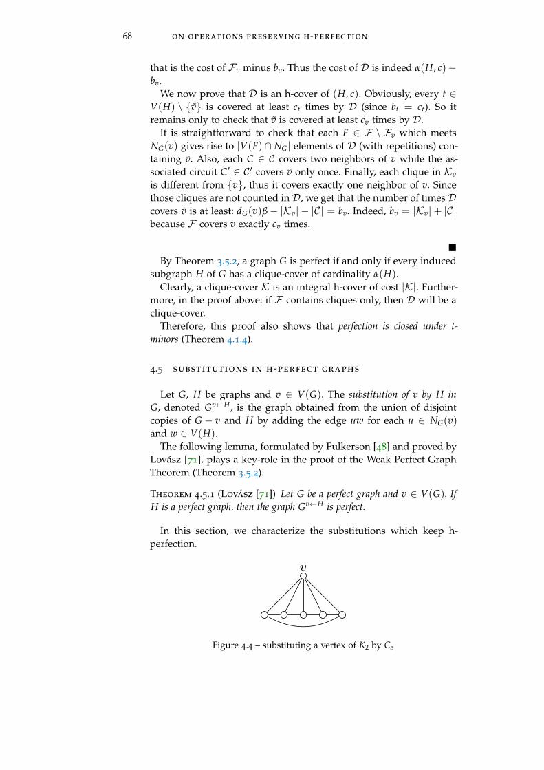
68 on operations preserving h-perfection
that is the cost of Fv minus bv. Thus the cost of D is indeed α(H, c)−bv.
We now prove that D is an h-cover of (H, c). Obviously, every t ∈V(H) \ {v} is covered at least ct times by D (since bt = ct). So itremains only to check that v is covered at least cv times by D.
It is straightforward to check that each F ∈ F \ Fv which meetsNG(v) gives rise to |V(F) ∩ NG| elements of D (with repetitions) con-taining v. Also, each C ∈ C covers two neighbors of v while the as-sociated circuit C′ ∈ C ′ covers v only once. Finally, each clique in Kv
is different from {v}, thus it covers exactly one neighbor of v. Sincethose cliques are not counted in D, we get that the number of times Dcovers v is at least: dG(v)β− |Kv| − |C| = bv. Indeed, bv = |Kv|+ |C|because F covers v exactly cv times.
�By Theorem 3.5.2, a graph G is perfect if and only if every induced
subgraph H of G has a clique-cover of cardinality α(H).Clearly, a clique-cover K is an integral h-cover of cost |K|. Further-
more, in the proof above: if F contains cliques only, then D will be aclique-cover.
Therefore, this proof also shows that perfection is closed under t-minors (Theorem 4.1.4).
4.5 substitutions in h-perfect graphs
Let G, H be graphs and v ∈ V(G). The substitution of v by H inG, denoted Gv←H, is the graph obtained from the union of disjointcopies of G − v and H by adding the edge uw for each u ∈ NG(v)and w ∈ V(H).
The following lemma, formulated by Fulkerson [48] and proved byLovász [71], plays a key-role in the proof of the Weak Perfect GraphTheorem (Theorem 3.5.2).
Theorem 4.5.1 (Lovász [71]) Let G be a perfect graph and v ∈ V(G). IfH is a perfect graph, then the graph Gv←H is perfect.
In this section, we characterize the substitutions which keep h-perfection.
v
Figure 4.4 – substituting a vertex of K2 by C5

4.5 substitutions in h-perfect graphs 69
It is not true in general that substitutions by perfect graphs keeph-perfection. Indeed, substituting a K2 for a vertex of C5 (which ish-perfect) yields the h-imperfect graph W−−5 (see Proposition 4.3.2).Furthermore, substituting an odd hole to a vertex of K2 yields an oddwheel W2k+1 with k ≥ 2 (see Figure 4.4) and we have (see Section 3.6.1for a proof):
Proposition 3.6.5 For each k ≥ 1, the graph W2k+1 is t-imperfect.
Further details on the stable set polytope of odd wheels can befound in Chapter 5.
We use only the polyhedral characterization of perfect graphs toprove our substitution theorem.
Obviously, if G is h-perfect and v is an isolated vertex of G, thenGv←H is h-perfect if and only if H is h-perfect too.
Theorem 4.1.5 Let G be an h-perfect graph, v be a non-isolated vertex ofG and H be a graph. The graph Gv←H is h-perfect if and only if at least oneof the following statements holds:
i) H has no edge,ii) H is perfect and v does not belong to an odd hole of G.
Proof – Let G′ := Gv←H. We first prove the "only if" part of thestatement.
only if: Suppose that G′ is h-perfect and that H has an edge.Clearly, an odd hole of H would yield an induced W2k+1 of G′ with
k ≥ 2, contradicting the h-perfection of G′.Hence, H has no odd hole. Since H is an induced subgraph of G′,
it is h-perfect and this implies that H is perfect (see Section 3.6.1).To see that v does not belong to an odd hole of G, observe that G′
would otherwise have an induced subgraph which can be t-contractedto W−−5 , contradicting the h-perfection of G (Proposition 4.3.2).
We now show the "if" part of the theorem.If: The result is trival if H has at most one vertex, so we may hence-
forth assume that |V(H)| ≥ 2.Let d ∈ Z
V(G′)+ . We prove:
α(G′, d) = ρhf (G
′, d). (4.2)
By Proposition 3.6.7, this will imply the h-perfection of G′. Since theinequality ≤ always holds, we need only to show the converse.
Let dH be the restriction of d to V(H). Now, let c ∈ ZV(G)+ be defined
as follows: for every t ∈ V(G), ct := α(H, dH) if t = v and ct := dt
otherwise. It is straightforward to check that α(G′, d) = α(G, c).Since G is h-perfect, Proposition 3.6.7 implies:
α(G′, d) = ρhf (G, c). (4.3)

70 on operations preserving h-perfection
Let y be a fractional rational h-cover of (G, c) of cost ρhf (G, c) (see
Section 3.6.2) and let k be a positive integer such that ky is integral.Let F be the integral h-cover of (G, kc) corresponding to ky.
Depending on whether condition i) or ii) of the statement of thetheorem holds, we build an integral h-cover F ′ of (G′, kd) of the costof F .
This construction will indeed end the proof of the "if" part of thetheorem: it implies kρh
f (G, c) ≥ ρhf (G
′, kd) and since ρhf (G
′, kd) ≥kρh
f (G′, d) (this is straightforward), we obtain ρh
f (G, c) ≥ ρhf (G
′, d).By (4.3), this shows α(G′, d) ≥ ρh
f (G′, d) and we finally get (4.2) as
required.
Case 1. H has no edge. Clearly, by induction on |V(H)| we only needto check the case |V(H)| = 2, so put V(H) = {u, w}.
Since v belongs to kcv elements of F and kcv = kdu + kdw, wecan choose a sub-multiset Fu of F with kdu elements all containingv. Then, there is a sub-multiset Fw of F − Fu of kdw elements allcontaining v.
Let F ′u := {F− v + u : F ∈ Fu} and F ′w := {F− v + w : F ∈ Fw}.The multiset F ′ := F ′u + F ′w + (F − Fu −Fw) is clearly an integralh-cover of (G′, kd) of the same cost as F .
Case 2. H is perfect and v does not belong to an odd hole of G. Here, Fv
only contains cliques. By definition, it has at least kα(H, dH) elements.Let r := α(H, dH). Since H is perfect, (H, dH) has a clique-cover
formed by r cliques K1, . . . , Kr (Theorem 3.5.2).Let K := {K′1, . . . , K′r} be a sub-multiset of Fv with kr elements and
let F ′ be obtained from F by replacing in K the clique K′i by the setK′i ∪ Ki of G′ for every i ∈ [r].
In G′, every vertex of H is adjacent to every neighbor of v in G.Thus, the sets Ki ∪ K′i are cliques of G′ and F ′ is an integral h-coverof (G′, kd) which has the same cost as F .
�A general result of Chvátal [26] shows that the stable set poly-
tope of Gv←H can be obtained from descriptions for STAB(G) andSTAB(H). This result can be used to give another proof of the "if"part of our result.
The proof above directly shows however that the theorem remainstrue if we replace h-perfection with strong h-perfection. Specializing Theo-rem 4.1.5 to K4-free graphs, it is straightforward to prove:
Corollary 4.5.2 Let G be a (strongly) t-perfect graph, v be a non-isolatedvertex of G and H be a graph. The graph Gv←H is (strongly) t-perfect if andonly if at least one of the following statements holds:
i) H has no edge,ii) v does not belong to an induced odd circuit of G and H is bipartite.

4.6 homogeneous sets in minimally h-imperfect graphs 71
4.6 homogeneous sets in minimally h-imperfect graphs
In this section, we show that Theorem 4.1.5 has a simple conse-quence for the structure of h-imperfect graphs which are minimalwith respect to t-minors.
Recall that a graph G is minimally h-imperfect (resp. minimally t-imperfect) if it is h-imperfect (resp. t-imperfect) and every proper t-minor of G is h-perfect (resp. t-perfect).
A module of a graph G is a subset X ⊆ V(G) such that every v ∈V(G) \ X satisfies NG(v) ⊇ X or NG(v) ∩ X = ∅. The trivial modulesof G are ∅, V(G) and the singletons of V(G) (they clearly are modulesof G). An homogeneous set of G is a non-trivial module of G. A graphis prime if it has no homogeneous set.
The graph W−−5 is minimally h-imperfect (see Theorem 5.1.4) andhas an homogeneous clique of cardinality two. We prove that it is theonly minimally h-imperfect graph which is not prime.
Theorem 4.1.6 Except W−−5 , every minimally h-imperfect graph is prime.
Proof – Let G be a minimally h-imperfect graph and suppose that Ghas an homogeneous set X. We show that W−−5 is a t-minor of G andthis will obviously prove the theorem.
Put H := G [X]. Let v ∈ X and put X′ := X− v. Since X is homoge-neous, G is obtained from G− X′ by substituting v by H. Besides, Gis minimally h-imperfect thus G− X′ is h-perfect.
Therefore, H must have an edge: otherwise Theorem 4.1.5 wouldimply that G is h-perfect, contradicting our assumption.
Let u ∈ V(G) \ X. The graph G − u is h-perfect and is obtainedfrom G− u− X′ by substituting v by H, which has at least one edge.Thus, another application of Theorem 4.1.5 shows that H is perfectand v does not belong to an odd hole of G− u− X′.
On the other hand, G is h-imperfect. Therefore, Theorem 4.1.5 im-plies that v must belong to an odd hole C of G− X′.
Since H has at least an edge, v has a neighbor w in X. As C isinduced, it contains exactly two neighbors of v in G− X′. Now, everyneighbor of v is adjacent to w and therefore G [V(C) + w] can be t-contracted to W−−5 . This shows that W−−5 is a t-minor of G.
�Specializing our result to minimally t-imperfect graph, we directly
obtain:
Corollary 4.6.1 K4 is the only non-prime minimally t-imperfect graph.


5M I N I M A L H - I M P E R F E C T I O N
T-perfection is in co-NP (Theorem 3.6.20) but no combinatorial certificateof t-imperfection is known.
Gerards and Shepherd [51] showed that t-perfection is closed for t-minors.A t-imperfect graph is minimally t-imperfect if all its proper t-minors are t-perfect. Hence, a graph is t-imperfect if and only if it has a t-minor which isminimally t-imperfect.
Therefore , studying minimally t-imperfect graphs may hopefully yield acombinatorial certificate of t-imperfection and provide a solid basis towardsunderstanding the complexity of deciding t-perfection.
For example, Bruhn and Stein [16] determined every minimally t-imperfectclaw-free graphs. Bruhn and Schaudt [14] used this to show a polynomial-time algorithm testing t-perfection in claw-free graphs.
Several minimally t-imperfect graphs have been identified by Shepherd[108] and Bruhn, Stein [13, 16].
In this chapter, we will first review the known examples of minimally t-imperfect graphs. We do not provide new ones, but give a description of theirstable set polytope and formulate a related conjecture. Moreover, we stateknown and new conjectures and further questions on minimally t-imperfect graphs.
Clearly, K4 is the only minimally t-imperfect graph which is not min-imally h-imperfect. In a second part, we prove that there are exactly threeminimally h-imperfect K4-free graphs which are not minimally t-imperfect: K∗4 ,W−5 and W−−5 . These graphs show that conjectures stated for minimally t-imperfect graphs have to be reformulated in order to extended to minimallyh-imperfect graphs.
It is not known whether h-perfection is in NP or co-NP. We state a con-jecture of Sebo (personal communication) whose validity would imply thatodd antiholes with at least 9 vertices are the only minimally h-imperfectgraphs having cliques of cardinality larger than 3. In particular, it wouldput h-perfection in co-NP.
We prove that the conjecture holds for a proper superclass of planar graphs.Webs form a class of claw-free graphs containing the odd antiholes. Wedetermine the h-perfect and minimally h-imperfect webs. Our results hopefullysimplify the still open task of characterizing minimally h-imperfect claw-free graphs.
Finally, we use the forbidden-induced-subgraph characterization of Caoand Nemhauser (Theorem 3.8.2) to determine the minimally h-imperfectline-graphs.
La t-perfection est une propriété co-NP (Théorème 3.6.20) mais on neconnaît pas de certificat combinatoire de t-imperfection.
Gerards et Shepherd [51] ont montré que les t-mineurs conservent la t-perfection. Un graphe t-imparfait est minimalement t-imparfait si tous ses t-mineurs propres sont t-parfaits. Ainsi, un graphe est t-imparfait si et seule-ment s’il a un t-mineur qui est minimalement t-imparfait.
73

74 minimal h-imperfection
Dès lors, la caractérisation des graphes minimalement t-imparfaits fournitune approche possible pour obtenir un certificat combinatoire de t-imperfection.Elle donnerait aussi une base solide pour l’étude de la complexité de la re-connaissance des graphes t-parfaits.
Par exemple, Bruhn et Stein [16] ont déterminé les graphes minimalementt-imparfaits sans griffe. Bruhn et Schaudt [14] ont utilisé ce résultat dans leuralgorithme polynomial de reconnaissance des t-parfaits dans la classe desgraphes sans griffe.
Plusieurs autres exemples de graphes minimalement t-imparfaits ont étédonnés par Shepherd [108] et Bruhn, Stein [13, 16].
Dans ce chapitre, nous faisons d’abord l’inventaire des exemples connusde graphes minimalement t-imparfaits et décrivons leur polytope des stables.Nous ne proposons pas de nouvel exemple mais sommes conduits à énon-cer une conjecture sur le polytope des stables des graphes minimalementt-imparfaits. Par ailleurs, nous énumérons plusieurs conjectures connues eten suggérons de nouvelles sur les propriétés combinatoires de ces graphes.
Il est facile de vérifier que K4 est l’unique graphe minimalement t-imparfaitqui n’est pas minimalement h-imparfait. Dans la seconde partie du cha-pitre, nous prouvons qu’il y a exactement trois graphes sans K4 minimalementh-imparfaits qui ne sont pas minimalement t-imparfaits : K∗4 , W−5 et W−−5 . Cesgraphes montrent que les conjectures formulées pour les minimalement t-imparfaits doivent être modifiées pour être étendues aux minimalement h-imparfaits.
L’appartenance de la h-perfection à NP ou co-NP est toujours ouverte.Nous énonçons une conjecture de Sebo (communication personnelle) affir-mant que les anti-trous impairs à au moins 9 sommets sont exactement lesgraphes minimalement h-imparfaits qui contiennent K4. La validité de cetteconjecture placerait directement la h-perfection dans co-NP.
Nous prouvons que cette conjecture est satisfaite par une classe contenant(strictement) les graphes planaires. Les graphes circulants forment une sous-classe des graphes sans griffe qui contient tous les anti-trous impairs. Oncaractérise les graphes circulants h-parfaits et minimalement h-imparfaits.Nous expliquons en quoi ces résultats pourraient être utiles dans la re-cherche d’une preuve de la conjecture de Sebo pour le cas des graphes sansgriffe.
Enfin, nous utilisons la caractérisation par sous-graphes-induits interditsdes graphes h-parfaits adjoints due à Cao et Nemhauser (Théorème 3.8.2)pour déterminer tous les graphes adjoints minimalement t-imparfaits.
5.1 introduction
T-perfection belongs to co-NP but a combinatorial certificate of t-imperfection is not known (Theorem 3.6.20). Whether t-perfection be-longs to NP is open.
The Strong Perfect Graph Theorem (Theorem 1.1.2) shows that im-perfection can be certified by showing an odd hole or odd antihole.It is easy to check that a graph is an odd hole or odd antihole, andthis places perfection in co-NP (a simpler certificate is provided bya theorem of Lovász [102, pg. 1109]). Odd holes and antiholes are

5.1 introduction 75
the minimally imperfect graphs: they are imperfect and their properinduced subgraphs are all perfect.
This suggests using operations which keep t-perfection and reducethe size of the graph in the process of seeking a combinatorial co-NPcharacterization of t-perfection.
Recall that a t-minor of a graph G is any graph obtained from G bya sequence of vertex-deletions and t-contractions. It is proper if it isdifferent from G.
Gerards and Shepherd [51] proved that t-perfection is closed under t-minors. A t-imperfect graph is minimally t-imperfect (abbreviated MTI)if all its proper t-minors are t-perfect. Hence, a graph is t-imperfect ifand only if it has an MTI t-minor.
A combinatorial algorithm recognizing minimally t-imperfect (orminimally h-imperfect) graphs would directly imply a combinatorialcertificate of t-imperfection (or h-imperfection).
The claw is the graph shown in Figure 5.1. A graph is claw-free if itdoes not have an induced claw. It is straightforward to check that theclass of claw-free graphs is closed under t-minors.
Theorem 5.1.1 (Bruhn, Stein [16]) The minimally t-imperfect claw-freegraphs are K4, W5, C2
7 and C210.
Therefore, a claw-free graph is t-perfect if and only if it does not have oneof these graphs as a t-minor. This directly puts t-perfection of claw-freegraphs in co-NP and was used by Bruhn and Schaudt [14] to show apolynomial-time algorithm testing t-perfection in claw-free graphs.
In this chapter, we will first review the currently known MTI graphswhich can be found in [13, 15]. There are several infinite families ofsuch graphs. No new example is provided and we do not know ifthere are more.
Figure 5.1 – the claw
An imperfect graph G is minimally imperfect if every proper inducedsubgraph of G is perfect. By the polyhedral characterization of perfec-tion (Theorem 3.5.3), STAB(G) must have a non-trivial facet which isnot defined by a clique-inequality of G. Furthermore, the polytopeQSTAB(G) described by the non-negativity and clique-inequalities ofG (see Section 3.5) must have a non-integral vertex. Padberg provedthe following:

76 minimal h-imperfection
Theorem 5.1.2 (Padberg, [89]) For every minimally imperfect graph G,the inequality x(V(G)) ≤ α(G) defines a facet of STAB(G) and:
STAB(G) =
x ∈ RV(G) :x ≥ 0,
x(K) ≤ 1 ∀K clique of G,
x(V(G)) ≤ α(G).
.
Furthermore, 1ω(G)
1 is the unique non-integral vertex of QSTAB(G).
In this context, Shepherd [107] called a graph G near-perfect if thenon-trivial facets of STAB(G) are defined by clique-inequalities orthe full-rank inequality x(V(G)) ≤ α(G). Hence, both perfect graphsand minimally imperfect graphs are near-perfect. In general, it is nottrue that the complement of a near-perfect graph is near-perfect (seeFigure 1.3). In [107], Shepherd showed that a graph G is minimallyimperfect if and only if G and G are near-perfect.
This motivates the definition of an analogous notion for h-perfection.We say that a graph G is near-h-perfect if STAB(G) is described bynon-negativity, clique and odd-circuit inequalities and the full-rankinequality of G. Near-h-perfect graphs include near-perfect and h-perfect graphs.
An h-imperfect graph is minimally h-imperfect (abbreviated MHI) ifall its proper t-minors are h-imperfect. In Chapter 4, we showed thath-perfection is closed under t-minors. Therefore, a graph is h-perfectif and only if it does not have an MHI t-minor.
In this chapter, we will show that except odd wheels W2n+1 (with n ≥2) and K∗4 (see Figure 5.2), the known examples of MHI graphs are near-h-perfect. Hence, we conjecture the following:
Conjecture 5.1.3 Except K∗4 and the odd wheels W2n+1 with n ≥ 2, everyminimally h-imperfect graph is near-h-perfect.
We will survey questions of Bruhn and Stein [16] (and ask newones) related to MTI graphs.
Clearly, K4 is the only MTI graph which is not MHI. There areK4-free MHI graph which are not MTI (they have K4 as a t-minor)and we determine all of them (see Figure 5.2 for the definitions of K∗4 ,W−5 , W−−5 ):
Theorem 5.1.4 The only K4-free minimally h-imperfect graphs are K∗4 , W−5and W−−5 .
These graphs are precisely those involved in Theorem 4.3.1 of Chap-ter 4. They also show that some of the conjectures formulated for MTIgraphs do not hold for MHI graphs in general.
On the other hand, we study minimally h-imperfect graphs withcliques of cardinality at least 4. Odd antiholes with at least 7 ver-tices form a class of minimally imperfect graphs with arbitrarily large

5.1 introduction 77
(a) K∗4 (b) W−5 (c) W−−5
Figure 5.2 – the graphs K∗4 , W−5 and W−−5
clique number. Theorem 5.1.2 shows that they are also MHI (seeProposition 5.4.4 for a direct proof).
Can a characterization of h-perfect graphs be reduced to one fort-perfect graphs ? Sebo (personal communication) conjectures the fol-lowing: a graph G is h-perfect if and only if every K4-free induced subgraphof G is t-perfect and G has no odd antihole with at least 9 vertices.
An h-imperfect graph G is critically h-imperfect if every proper in-duced subgraph of G is h-perfect. Clearly, this conjecture states:
Conjecture 5.1.5 (Sebo) Every critically h-imperfect graph with ω ≥ 4is an odd antihole.
Since MHI graphs are critically h-imperfect, it would imply thatthe MHI graphs are the MTI graphs (except K4), W−5 , W−−5 , K∗4 and theC2n+1 with n ≥ 4.
We say that a graph G is 4-clique-separated if each non-completeconnected induced subgraph H of G with ω(H) ≥ 4 has a vertex-cutwhich is a clique. It is easy to check that the class of 4-clique-separatedgraphs is closed under taking induced subgraphs and contains noodd antihole C2n+1 with n ≥ 4.
Tucker [116] proved that planar graphs are 4-clique-separated. We ob-serve that Conjecture 5.1.5 holds for the class of 4-clique-separatedgraphs in the simplest possible way:
Theorem 5.1.6 Critically h-imperfect 4-clique-separated graphs are K4-free.
In other words: a 4-clique-separated graph is h-perfect if and only if itsK4-free induced subgraphs are t-perfect.
Recall that for integers n ≥ 3 and k ≥ 1: Ckn denotes the graph
obtained from Cn by adding an edge between two vertices whosedistance (in the sense of shortest paths) on Cn is at most k.
The graphs Ckn are called webs (see Section 3.2.1). We prove:
Theorem 5.1.7 A web is h-perfect if and only if it is a circuit or a completegraph or a Ck
2k+2 with k ≥ 1.
Theorem 5.1.8 A web is critically h-imperfect if and only if it is C210 or an
odd antihole C2n+1 with n ≥ 3.

78 minimal h-imperfection
In particular, the critically h-imperfect webs which have cliques ofcardinality 4 are odd antiholes. Webs form a proper subclass of claw-free graphs and we do not know if Conjecture 5.1.5 further holds forthe latter. Still, our results on webs show that the conjecture for claw-free graphs is implied by the following statement (see Section 5.2.4for the definition of partitionable graphs):
Conjecture 5.1.9 Each critically h-imperfect claw-free graph with ω ≥ 4is partitionable.
Antiwebs (the complements of webs) also include odd antiholes,but we do not know if critically h-imperfect antiwebs which havecliques of cardinality 4 are odd antiholes. Antiwebs form a class ofnearly-bipartite graphs (that is each vertex has a neighbor in each oddcircuit). These graphs were studied by Shepherd in [108] (see alsoSection 5.2.2).
We end this chapter by observing that the characterization of h-perfect line-graphs by Cao and Nemhauser (Theorem 3.8.2) impliesa characterization of the minimal (under t-minors) h-imperfect line-graphs:
Theorem 5.1.10 The minimally h-imperfect line-graphs are W−5 and W−−5 .
Hence, a line-graph is h-perfect if and only if it does not have W−5 or W−−5as t-minor.
outline In Section 5.2, we review the known examples of MTIgraphs, state related properties and give a description of their respec-tive stable set polytope. In particular we show that, except odd wheelsW2n+1 with n ≥ 2, all these examples are near-h-perfect.
In Section 5.3, we mention questions and conjectures of Bruhn andStein for MTI graphs and give new ones. We also discuss the problemof finding more examples of MTI graphs.
In Section 5.4 we show that K∗4 , W−5 and W−−5 are the K4-free MHIgraphs which are not MTI. We describe the stable set polytope ofthese graphs and observe that the conjectures given for MTI graphsmust be reformulated to be extended to MHI graphs. Besides, weshow that Conjecture 5.1.5 holds for 4-clique-separated graphs.
In Section 5.5, we determine the h-perfect and critically h-imperfectwebs. We use these results to show that Conjecture 5.1.5 for claw-freegraphs would follow from Conjecture 5.1.9. We conclude the chapterby determining the MHI line-graphs.
5.2 a review of known minimally t-imperfect graphs .consequences and conjectures
Since t-perfection is closed under t-minors (Theorem 4.1.2), a graphG is MTI if and only if for every v ∈ V(G): G− v is t-perfect, and if v iscontractible then G/NG [v] is t-perfect.

5.2 a review of known minimally t-imperfect graphs 79
In this section, we review the currently known examples of MTIgraphs which can be found in [13, 15]. We do not provide new exam-ples.
Our contribution consists in finding a description of the stable setpolytope for each of these examples (when such a description isnot known). This led us to the formulation of the notion of near-h-perfection and a related conjecture. We will often use the followingresult:
Proposition 5.2.1 Let G be a critically h-imperfect graph and F be a non-trivial facet of STAB(G) which is not defined by a clique or odd-circuitinequality.
If aTx ≤ b is valid for STAB(G) and defines F, then a > 0. Furthermore,if every inclusion-wise maximal stable set is maximum, then
F = {x ∈ STAB(G) : x(V(G)) ≤ α(G)} ,
and G is near-h-perfect.
Proof – We first prove a > 0. Let G be a critically h-imperfect graphand suppose to the contrary that G has a vertex v such that av = 0.Let a′ be the restriction of a to V(G) \ {v}. It is straightforward tocheck that a′Tx ≤ b (over RV(G−v)) defines a facet of STAB(G − v).Since G is critically h-imperfect, a′Tx ≤ b is a clique or odd-circuitinequality of G− v (up to a positive scalar factor). Hence F is definedby a clique or odd circuit inequality of G: a contradiction.
Now, let us assume furthermore that every inclusion-wise maximalstable set of G is maximum and let Fα be the face of STAB(G) definedby the inequality x(V(G)) ≤ α(G). Since a > 0, every stable set S ofG satisfying a(S) = b is inclusion-wise maximal and thus has |S| =α(G).
In other words, every vertex of F belongs to Fα and thus F ⊆ Fα.Since F is a facet of STAB(G), we must have F = Fα.
�The currently known MTI graphs can be grouped into four fami-
lies.
5.2.1 Odd wheels
Let k ≥ 3 and Ck be the circuit of length k. The wheel graph of orderk, denoted Wk, is obtained by adding to Ck a new vertex c which isadjacent to every vertex of Ck (see Figure 5.3 for an example). Therim of Wk is the circuit corresponding to Ck and c is the center of Wk.Notice that Wk has k + 1 vertices.
Clearly, if k is even then Wk is almost-bipartite and Theorem 3.6.14
shows that it is t-perfect. By contrast, the following straightforwardstatement holds [102, pg. 1194]:

80 minimal h-imperfection
Figure 5.3 – the graph W5
Proposition 5.2.2 For each integer n ≥ 1, W2n+1 is minimally t-imperfect.
Since K4 = W3 is h-perfect, W2n+1 is MHI if and only if n ≥ 2. Propo-sition 5.2.2 and Proposition 5.2.1 yield the following well-known re-sult:
Proposition 5.2.3 Let n ≥ 2 be an integer and W be the wheel of size2n + 1. Let C be the rim and c be the center of W. The following holds:
STAB(W) =
x ∈ RV(W) :xv ≥ 0 ∀v ∈ V(W),
x(K) ≤ 1 for each triangle K of W,
nxc + x(V(C)) ≤ α(W).
.
Furthermore, each of the above inequalities defines a facet of STAB(W).
Proof – The non-negativity and inclusion-wise maximal clique in-equalities define facets of STAB(W) (see Section 3.4).
Clearly, α(W) = n and the inequality nxc + x(V(C)) ≤ n is valid forSTAB(W). The 2n + 1 stable sets of cardinality n of C form, togetherwith {c}, a set of 2n + 2 affinely independent stable sets of W whichare tight for this inequality. Hence it defines a facet of STAB(W).
Suppose by contradiction that aTx ≤ b defines a non-trivial facet Fof STAB(W) which is not defined by a clique or odd-circuit inequalityor nxc + x(V(C)) ≤ n.
It is easy to check that since F is not defined by a triangle inequalityof W, a must be constant on the rim.
Since G is critically t-imperfect, Proposition 5.2.1 shows that a > 0and thus we may assume without loss of generality that av = 1 forevery v ∈ V(C).
Furthermore, there must exists a stable set S of W such that a(S) =b and n|S∩{c} |+ |S \ {c} | ≤ n− 1. Hence, c /∈ S and b = |S| ≤ n− 1.Since aTx ≤ b is valid for STAB(W), we also have b ≥ α(C) = n: acontradiction.
This shows that STAB(G) is described by non-negativity, clique-inequalities, x(V(C)) ≤ n and nxc + x(V(C)) ≤ n. Besides, it is easyto check that there are only 2n stable sets of G which are tight forx(V(C)) ≤ n. Therefore, it does not define a facet of G.

5.2 a review of known minimally t-imperfect graphs 81
�In particular, K4 is the only near-h-perfect odd wheel. We end this
section with the following consequence of Proposition 5.2.2 for criti-cally h-imperfect graphs.
Corollary 5.2.4 A critically h-imperfect graph which is not an odd wheelW2n+1 (with n ≥ 2) is such that each neighborhood induces a perfect graph.
Proof – Suppose that G has a vertex v such that G [NG(v)] is im-perfect. Since this graph is a proper induced subgraph of G, it is h-perfect and must have an odd hole. Hence, G has an induced W2n+1
with n ≥ 2 and, by criticality, must be isomorphic to it.
�This result further holds for MHI graphs as they are obviously
critically h-imperfect.
5.2.2 Even Möbius Ladders
Let k ≥ 2, P := (u1, . . . , uk) and Q := (v1, . . . , vk) be two vertex-disjoint copies of Pk. Let Mk be the graph obtained by taking theunion of P and Q and adding the edges u1vk, v1uk and uivi for eachi ∈ [k]. The graph Mk is the Möbius ladder of size k and has 2k vertices(see Figure 5.4). A Möbius ladder Mk is even if k is even. For example,M2 = K4. These graphs were introduced in the context of t-perfectionby Shepherd [108].
(a) M4 (b) M6
1
2
1
22
1
1
2
2
1
(c) M5
Figure 5.4 – examples of Möbius ladders and a 2-vertex-coloring of M5

82 minimal h-imperfection
When k is odd, the graph Mk is bipartite (see Figure 5.4.c)). Thedescription of the stable set polytope of even Möbius ladders followsfrom a general result of Shepherd for nearly-bipartite graphs.
A graph G is nearly-bipartite if for every vertex v of G, the graph G−NG [v] is bipartite. Clearly, every Möbius ladder is nearly-bipartite.
An antiweb is the complement of a web, and Ckn denotes the comple-
ment of the web Ckn (for integers k ≥ 1 and n ≥ 3). See Section 3.2.1
for the definition of webs. Obviously, antiwebs are regular graphs.An antiweb Ck
n is prime if n ≥ 2k + 2, and k + 1 and n are relativelyprime. For each odd integer k ≥ 3, the even Möbius ladder Mk+1 isthe prime antiweb Ck−1
2k+2 (see [108] for details). Besides, C2l+1 (with
l ≥ 2) is clearly isomorphic to the prime antiweb Ck−12k+1.
Let G be a graph. A set-join of G is a set {X1, . . . , Xl} of pairwise-disjoint (possibly empty) subsets of vertices of G such that for all1 ≤ i < j ≤ l and for each (u, v) ∈ Xi × Xj, we have uv ∈ E(G). Itis furthermore prime if each Xi is either a clique or induces a primeantiweb. Finally, the inequality of G associated to a set-join {X1, . . . , Xl}is:
l
∑i=1
1α(G [Xi])
x(Xi) ≤ 1.
Clearly, this inequality is valid for STAB(G). Shepherd proved thefollowing:
Theorem 5.2.5 (Shepherd, [108]) If G is a nearly-bipartite graph, thenthe non-trivial facets of STAB(G) are defined by inequalities of prime set-joins.
We use this result to simultaneously prove that the even Möbius lad-ders are MTI (their critical t-imperfection is stated by Shepherd in[108]) and give a description of their stable set polytope.
Corollary 5.2.6 The even Möbius ladders are minimally t-imperfect andnear-h-perfect.
Proof – Put M := M2k with k ≥ 2 (M2 is just K4). Clearly, M is 3-regular and connected. Hence, its regular proper induced connectedsubgraphs must be 2-regular. Besides, it is easy to check that 2-regularprime antiwebs are odd holes.
Therefore, the proper induced subgraphs of M which are primeantiwebs are its odd holes.
Obviously, M does not contain odd wheels. Thus, the prime set-joins of M are the cliques, the odd holes of M and M itself.
Hence, Theorem 5.2.5 shows that the non-trivial facets of STAB(M)
are defined by cliques, odd-circuit inequalities and x(V(M)) ≤ α(M).In other words, M is near-h-perfect.
Since being nearly-bipartite is clearly closed under taking inducedsubgraphs, Theorem 5.2.5 also shows that M is a critically t-imperfect

5.2 a review of known minimally t-imperfect graphs 83
graph. Hence, it remains only to prove that every t-contraction of Mis t-perfect.
Since M is clearly vertex-transitive and every vertex of M is con-tractible, we need only to show that M/NM [v] is t-perfect for some ar-bitrary v ∈ V(M). Let v be the new vertex of M/NM [v]. It is straight-forward to check that (M/NM [v])− v is bipartite. Hence M/NM [v]is almost-bipartite and thus Theorem 3.6.14 shows that it is t-perfect.
�Shepherd showed as a corollary of Theorem 5.2.5 that:
Theorem 5.2.7 (Shepherd [108]) A nearly-bipartite graph is t-perfect ifand only if it does not have an induced odd wheel or an induced primeantiweb which is not an odd hole.
Hence, the MTI nearly-bipartite graphs are odd wheels and MTIprime antiwebs. As we have seen above, prime antiwebs include theeven Möbius ladders. In Section 5.2.4, we will see that there is at leastone other example of an MTI prime antiweb: C2
10. We do not know ifthere are more.
5.2.3 Squares of circuits
Dahl [32] gave a complete description of STAB(C2n) for each integer
n ≥ 3. Bruhn and Stein [16] proved that K4 is a t-minor of C2n for each
n ≥ 5 which is not 6, 7 or 10.It is straightforward to check that C2
6 is perfect (and thus t-perfect)and that C2
7 is MTI (the latter also follows from Theorem 5.1.2 byobserving that C2
7 = C7).
Theorem 5.2.8 (Bruhn, Stein [16]) Let n ≥ 3 be an integer. The follow-ing statements hold:
a) C2n is t-perfect if and only if n ∈ {3, 6},
b) C2n is minimally t-imperfect if and only if n ∈ {4, 7, 10}.
(a) C27 (b) C2
10
Figure 5.5 – the minimally t-imperfect graphs C27 and C2
10
Since C27 = C7, Theorem 5.1.2 shows:
Corollary 5.2.9 C27 is near-perfect.

84 minimal h-imperfection
Finally, the near-h-perfection of C210 is a direct consequence of re-
sults of Dahl [32, Lemma 3.2 and Theorem 3.3, pg. 9-10].
Proposition 5.2.10 C210 is near-h-perfect.
5.2.4 Partitionable graphs
A graph G is partitionable if |V(G)| = α(G)ω(G) + 1 and for everyv ∈ V(G): G − v has a partition into ω(G) stable sets which are allof cardinality α(G) and a partition into α(G) cliques which are all ofcardinality ω(G). It is easy to check that each partitionable graph Gsatisfies α(G) ≥ 2 and ω(G) ≥ 2.
For integers p ≥ 2 and q ≥ 2, a (p, q)-graph is a partitionable graphwith α(G) = p and ω(G) = q.
In this section, we review known examples of MTI partitionablegraphs and observe that they are near-h-perfect.
Clearly, partitionability only depends on the underlying simplegraph. Hence, we need only to consider simple graphs.
The class of partitionable graphs plays a key-role in the study ofperfect graphs. By a theorem of Lovász [71], every minimally imperfectgraph is partitionable.
It is an easy exercise to check that the (p, 2)-graphs are the odd holes.Hence, they are all t-perfect. By contrast:
Proposition 5.2.11 Each partitionable graph G with ω(G) ≥ 3 is h-imperfect.
Proof – Clearly, the vector x := 1ω(G)
belongs to HSTAB(G) and
x(V(G)) =13(α(G)ω(G) + 1) > α(G).
Hence, x /∈ STAB(G) and G is h-imperfect.
�Obviously, each (p, 4)-graph is not MTI. Hence, the MTI partition-
able graphs are (p, 3)-graphs.Shepherd showed an algorithm testing partitionability [92, chap.
12], but it is still difficult in general to produce explicit examplesof partitionable graphs [11]. The (p, 3)-graphs with p ≤ 3 are well-known however and we review these graphs below.
Clearly, the only MTI (2, 3)-graph is C7 (that is C27). We now review
(3, 3)-graphs.An edge of a (p, q)-graph G is undetermined if it is not an edge of a
maximum clique of G (that is a clique of cardinality q).A (p, q)-graph is normalized if it has no undetermined edge. For
each normalized partitionable graph H, let U(H) denote the set ofnon-adjacent pairs of vertices uv of H such that each maximum cliqueof H + uv is a clique of H.

5.2 a review of known minimally t-imperfect graphs 85
Chvátal, Graham, Whitesides and Perold [27] observed that for each(p, q)-graph G and each undetermined e ∈ E(G): the maximum stable setsof G− e are maximum stable sets of G.
In particular, G− e is a (p, q)-graph. This shows that each (p, q)-graphis of the form H + F, where H is a normalized (p, q)-graph and F ⊆ U(H).
Let D be the graph of Figure 5.6. It is straightforward to check thatD is a normalized (3, 3)-graph. This graph was found by Huang [10]and Chvátal et al. [27].
Theorem 5.2.12 (Chvátal et al. [27]) The normalized (3, 3)-graphs areC2
10 and D.
u
v
(a) D
v1
v2
v3
v4
v5v6
v7
v8
v9
v10
(b) C210
Figure 5.6 – the two normalized (3, 3)-graphs
Clearly, U(D) = {uv} (see Figure 5.6) and U(C210) is the set of
diagonals vivi+5 with i ∈ [5]. The graphs obtained by adding (as edges)pairs from U(D) and U(C2
10) to D and C210 respectively are shown in
Figure 5.7 and Figure 5.8.Clearly, they all are (3, 3)-graphs. Besides, it is straightforward to
check that D+ = D, C210(5) = C2
10, C210(3) = C2
10(2)′, C2
10(3)′ = C2
10(2)and C2
10(4) = C210(1).
Therefore:
Corollary 5.2.13 (Chvátal et al. [27]) The (3, 3)-graphs are D, C210,
C210(1), C2
10(2), C210(2)
′ and their complements.
Bruhn and Stein proved that all these graphs are MTI and showed thatthey are minimally strongly t-imperfect: they are t-imperfect and theirproper t-minors are strongly t-perfect.
Theorem 5.2.14 (Bruhn, Stein [13, 15]) The (3, 3)-graphs are minimally(strongly) t-imperfect.
The situation for (4, 3)-graphs is different. Indeed, a normalized(4, 3)-graph found by Chvátal et al. [27] has a proper induced W7 [27,graph of Figure 6 pg. 89]. Hence, it is not MTI.

86 minimal h-imperfection
(a) C210 (b) C2
10(1) (c) C210(2)
(d) C210(2)
′ (e) C210(3) (f) C2
10(3)′
(g) C210(4) (h) C2
10(5)
Figure 5.7 – the (3, 3)-graphs obtained from C210
(a) D (b) D+
Figure 5.8 – the (3, 3)-graphs obtained from D
We show that the (3, 3)-graphs are near-h-perfect. Since the inclusion-wise maximal stable sets of C2
10 and D are maximum, Proposition 5.2.1directly implies:
Proposition 5.2.15 C210 and D are near-h-perfect.
Besides, the near-h-perfection of C210 follows from results of Dahl
[32] (see Proposition 5.2.10).

5.2 a review of known minimally t-imperfect graphs 87
The other (3, 3)-graphs obtained from C210 and D have maximal sta-
ble sets which are not maximum. Even though our proofs for eachof these graphs are similar, we do not know of a more general argu-ment which would imply their near-h-perfection all-at-once. As anexample, we present here the proof for C2
10(1).
Proposition 5.2.16 The graph C210(1) is near-h-perfect.
Proof – Put G := C210(1). We will use the vertex-numbering of Fig-
ure 5.9. By contradiction, suppose that STAB(G) has a non-trivialfacet F which is not defined by a clique or odd-circuit inequality orx(V(G)) ≤ α(G). Let aTx ≤ b be a valid inequality for STAB(G)
defining F.Since G is MTI (by Theorem 5.2.14), Proposition 5.2.1 shows that
a > 0. Put M := maxv∈V(G) av and let T := {v ∈ V(G) : av = M}. Wewill prove that T = V(G). This will imply that b = M · α(G) andcontradict that F is not defined by x(V(G)) ≤ α(G).
Since F is not defined by x(V(G)) ≤ α(G) and as α(G) = 3, G hasa stable set S0 such that |S0| ≤ 2 and a(S0) = b. Since a > 0, S0 isinclusion-wise maximal. Obviously, we must have S0 = {v1, v6} (thatis the only non-adjacent diagonal pair).
We claim that S0 ∩ T 6= ∅. Indeed, let v ∈ V(G) such that av = M.Clearly v is a neighbor of v1 or v6, say v6 (by horizontal symmetry).Then {v1, v} is a stable set and av1 + av ≥ a(S0) = b, thus av1 + av = b.Therefore, av6 = av = M and v6 ∈ T.
By symmetry, we may henceforth assume that v6 ∈ T. Since F isnot defined by the clique inequality of K := {v6, v7, v8}, G has aninclusion-wise maximal stable set S1 such that a(S1) = b and S1 ∩{v6, v7, v8} = ∅. This implies that S1 = {v2, v5, v9}. Now, S1− v5 + v6
is a stable set thus: a(S1− v5 + v6) ≤ b, which implies that av5 ≥ av6 =
M. Hence, v5 ∈ T.The same argument used successively with the clique {v5, v6, v7}
(resp. {v4, v5, v6}) instead of K yields v4, v7 ∈ T (resp. v3 ∈ T). Now,we also have v1 ∈ T. Indeed, {v6, v3} is a stable set and since v3 ∈ T:av6 + av3 ≥ av6 + av1 = b, thus av1 = av3 = M.
Finally, b = a(S0) = av1 + av6 = 2M because v1, v6 ∈ T. However{v1, v4, v7} is a stable set contained in T, hence a({v1, v4, v7}) = 3M ≤2M. This is absurd.
�The proofs for the other (3, 3)-graphs follow the same plan. We do
not include them as they do not clearly provide further informationon how to build a general argument.
Theorem 5.2.17 The (3, 3)-graphs are near-h-perfect.

88 minimal h-imperfection
v1
v2
v3
v4
v5v6
v7
v8
v9
v10
Figure 5.9 – denoting the vertices of C210(1) for the proof of Proposi-
tion 5.2.16
5.3 conjectures and questions on minimally t-imperfect
graphs
The currently known MTI graphs are (see the previous section):
odd wheels, even Möbius ladders, C27 and the (3, 3)-graphs (∗)
We do not know if this list is complete. More examples of MTI graphsmay be found by investigating t-perfection in particular families ofgraphs which are closed under t-minors (see the next section). Forexample: K4, W5, C2
7 and C210 are the MTI claw-free graphs [16].
In this section, we list known and new conjectures, and questionswhich may motivate further research on MTI graphs.
connectivity Recall that a vertex-cut of a connected graph G isa set X ⊆ V(G) such that G− X is not connected. Clearly, each MTIgraph is connected and has no vertex-cut which is a clique (see Corol-lary 3.6.12). However, can two non-adjacent vertices of an MTI graphform a vertex-cut ? In other words:
Question 5.3.1 (Bruhn, Stein [16]) Is every minimally t-imperfect graph3-connected ?
In this context, it is worth mentioning the following result:
Theorem 5.3.2 (Bruhn, Stein [16]) Let G be a minimally t-imperfect graph.If G has a vertex-cut {u, v} formed by two non-adjacent vertices, then
G− u− v has exactly two connected components C1, C2. Furthermore, forexactly one i ∈ {1, 2}: G [Ci ∪ {u, v}] is a path between u and v.
This directly implies that if an MTI graph has no vertex of degree2, then it must be 3-connected. Therefore, Bruhn and Stein also askedthe following:
Question 5.3.3 (Bruhn, Stein [16]) Does every minimally t-imperfect graphhave minimum degree 3 ?

5.3 conjectures and questions on minimally t-imperfect graphs 89
All known examples obviously have minimum degree 3. In Sec-tion 5.4, we will see that this is not true for MHI graphs.
near-h-perfection In the preceding sections, we gave a descrip-tion of the stable set polytope of each MTI graph of the list (∗). Weobserved that, except odd wheels W2n+1 with n ≥ 2, these graphs arenear-h-perfect. Hence, we conjecture the following:
Conjecture 5.3.4 Except the odd wheels W2n+1 with n ≥ 2, every mini-mally t-imperfect graph is near-h-perfect.
If valid, this would provide an analog of Theorem 5.1.2 for min-imal t-imperfection. Furthermore, it would imply (through Proposi-tion 3.4.1) the following formula for the fractional chromatic numberof an MTI graph G which is not a W2n+1 with n ≥ 2 (see Section 3.6.4for the notation Γ):
χ f (G) = max(
ω(G), Γ(G),|V(G)|α(G)
).
In Section 5.4, we will see that the statement of Conjecture 5.3.4 doesnot hold for MHI graphs in general.
fractional chromatic number As clique and odd circuit in-equalities of a graph G are always valid for STAB(G), Proposition 3.4.1shows that every graph G satisfies χ f (G) ≥ max(ω(G), Γ(G)).
Besides, Proposition 3.6.15 states that equality holds when G is t-perfect. Bruhn (personal communication) conjectures that this prop-erty characterizes t-perfection.
Conjecture 5.3.5 (Bruhn) Every minimally t-imperfect graph G satis-fies:
χ f (G) > max(ω(G), Γ(G)).
It is straightforward to check that this holds for every graph in (∗).Now, if Conjecture 5.3.4 is valid then Conjecture 5.3.5 is equivalent
to the following statement: except the W2n+1 with n ≥ 2, every minimallyt-imperfect graph G satisfies:
|V(G)| > α(G) ·max(ω(G), Γ(G)).
This statement may be compared to the following characterization ofperfect graphs due to Lovász:
Theorem 5.3.6 (Lovász [71]) For every graph G, the following statementsare equivalent:
i) G is perfect,ii) every induced subgraph H of G satisfies |V(H)| ≤ α(H)ω(H).

90 minimal h-imperfection
vertices of TSTAB By Theorem 5.1.2, every minimally imper-fect graph G is such that QSTAB(G) has a unique non-integral ver-tex which is 1
ω (G)1.
Proposition 3.6.2 shows that if G is an MTI graph, then TSTAB(G)
has at least one non-integral vertex. Bruhn and Stein asked whetherthere could be more non-integral vertices of TSTAB(G):
Question 5.3.7 (Bruhn, Stein [16]) For a minimally t-imperfect graphG, does TSTAB(G) have precisely one non-integral vertex ?
It is not difficult to check that the answer is positive at least for theodd wheels, C2
7 and C210. We do not know if it holds for every MTI
graph of the list (∗). We will see in Section 5.4 that it does not holdfor two K4-free MHI graphs which are not MTI.
Finally, trying to extend the proof of Theorem 5.1.2 by Padberg ledus to ask:
Question 5.3.8 Can a minimally t-imperfect graph have both contractibleand non-contractible vertices ?
Question 5.3.9 Do the odd holes of a minimally t-imperfect graph all havethe same length ?
The answers to these questions are obviously positive for the graphsof the list (∗). In Section 5.4.1, we will see that the answer to Ques-tion 5.3.8 is positive for each K4-free MHI graph which is not MTI.
more mti graphs We end this section by discussing how otherexamples of MTI graphs might be found.
CLearly, the class of planar graphs is closed under t-minors. Amongthe known examples of MTI graphs, only the odd wheels (includingK4) and C2
10 are planar. Bruhn (personal communication) asks the fol-lowing:
Question 5.3.10 (Bruhn) Are there minimally t-imperfect planar graphsother than C2
10 and the odd wheels ?
We will show in Section 5.4.2 that the MHI planar graphs are K4-free and that characterizing h-perfect planar graphs can be easily re-duced to determining the t-perfect ones.
Let k ≥ 1 be an integer. A graph is Pk-free if it does not have aninduced Pk (see Section 3.2.1). It is straightforward to check that theclass of Pk-free graphs is closed under t-minors. Hence, the class ofPk-free graphs may be of interest for seeking new examples of MTIgraphs.
Esperet et al. [40] proved that every {P5, K4}-free graph is 5-colorable.Besides, a maximum-weight stable set can be found in polynomial-time inP5-free graphs [70].
The known MTI P5-free graphs are K4, W5, C27 and C2
10.

5.4 minimally h-imperfect graphs in general 91
Question 5.3.11 Are there minimally t-imperfect P5-free graphs other thanK4, W5, C2
7 and C210 ?
Sumner proved the following theorem:
Theorem 5.3.12 (Sumner, [111]) Each triangle-free P5-free graph is eitherbipartite, or obtained from C5 by substituting its vertices by stable sets.
Since substituting stable sets for vertices of a t-perfect graph keepst-perfection (Theorem 4.1.5), this implies:
Corollary 5.3.13 Every triangle-free P5-free graph is t-perfect.
5.4 minimally h-imperfect graphs in general
In this section, we first determine the K4-free MHI graphs whichare not MTI. Then, we give a description of their stable set polytope.Our results show that some of the conjectures and questions givenfor MTI graphs need to be reformulated for MHI graphs. Moreover,we state a conjecture of Sebo for critically h-imperfect graphs withcliques of cardinality 4 and prove it for 4-clique-separated graphs(which include planar graphs).
5.4.1 K4-free minimally h-imperfect graphs. Near-h-perfection and conjec-tures
We first show:
Theorem 5.1.4 The only K4-free minimally h-imperfect graphs are K∗4 , W−5and W−−5 .
Proof – The h-imperfection of K∗4 , W−5 and W−−5 is stated in Propo-sition 4.3.2. Furthermore, it is straightforward to check that everyproper t-minor of each of these graphs is formed by clique-sums ofodd circuits and complete graphs, thus it is h-perfect (Corollary 3.6.12).Therefore, they are MHI.
Conversely, let G be a K4-free MHI graph which is not MTI.Clearly, G is t-imperfect. Moreover for each v ∈ V(H): G − v is h-perfect and K4-free, thus it is t-perfect. Since G is not MTI, G musthave a contractible vertex u such that G/NG [u] is t-imperfect. Sinceh-perfection is closed under t-contractions (Theorem 4.1.3), G/NG [u]is h-perfect. Hence, G/NG [u] has a K4.
In particular, ω(G/NG [u]) > ω(G) and Proposition 4.3.6 impliesthat u must be a special vertex of an induced K∗4 , W−5 or W−−5 of G.Since G is MHI and each of these graphs is MHI, H must coincidewith one of them.
�

92 minimal h-imperfection
These graphs are precisely those appearing in our characterizationof graphs and contractible vertices for which t-contraction can beinterpreted as taking a face of HSTAB (Theorem 4.3.1). Besides, weproved that W−−5 is the only MHI graph which has an homogeneous set(see Theorem 4.1.6 in Chapter 4). Since the inclusion-wise maximalstable sets of W−5 and W−−5 are maximum, Proposition 5.2.1 implies:
Proposition 5.4.1 W−5 and W−−5 are near-h-perfect.
Let c denote the vertex of K∗4 which is not adjacent to its triangle(see Figure 5.10).
Proposition 5.4.2 The non-trivial facets of STAB(K∗4) are defined by clique,odd-circuit inequalities and the inequality
2xc + x(V(K∗4) \ {c}) ≤ 3, (5.1)
which defines a facet of STAB(K∗4).
Proof – Put G := K∗4 . In this proof, we speak of a maximal stable setto mean "inclusion-wise maximal".
The inequality (5.1) is obviously valid for STAB(G) and it is easyto find 7 tight linearly independent stable sets of G. Hence, it definesa facet of STAB(G).
Now, let F be a non-trivial facet of STAB(G) which is not defined bya clique or odd circuit-inequality. Let aTx ≤ b be a valid inequality ofSTAB(G) defining F. We will show that aTx ≤ b is a positive multipleof (5.1).
By Theorem 5.1.4, K∗4 is MHI. Hence, Proposition 5.2.1 shows thata > 0. We use the numbering of the vertices of G given in Figure 5.10.
c
v1 v2 v3
v5v4 v6
Figure 5.10 – notation for the vertices of K∗4
Since F is not defined by the inequality of the odd hole C :=cv2v5v4v1, there exists a stable set S of G such that a(S) = b and|S ∩ V(C)| < 2. Since a > 0, S is maximal and this implies thatS = {c, v6}. Hence ac + av6 = b. Using the same argument withthe other induced odd holes of G (all have length 5), we obtain:ac + av4 = ac + av5 = b. Therefore: av4 = av5 = av6 .
Since F is not defined by the clique-inequality of v4v5v6, there existsa maximal stable set S′ such that a(S′) = b and S′ ∩ {v4, v5, v6} = ∅.

5.4 minimally h-imperfect graphs in general 93
This implies that S′ = {v1, v2, v3}. Now S′ − v1 + v4 is a stable set ofG and aTx ≤ b is valid for STAB(G). Therefore, a(S′ − v1 + v4) ≤ band thus we get av4 ≤ av1 . Similarly, we obtain av5 ≤ av2 and av6 ≤ av3 .
Again, F is not defined by the inequality associated to the cliquecv1 so there is a maximal stable set S′′ such that a(S′′) = b and whichis disjoint from cv1. Clearly, v4 ∈ S′′ and S′′ − v4 + v1 is a stable set ofG. Hence a(S′′ − av4 + av1) ≤ a(S′′), that is av1 ≤ av4 .
We similarly show av2 ≤ av5 and av3 ≤ av6 . Therefore: av1 = av4 ,av2 = av5 and av3 = av6 .
The equalities obtained yield that: avi = avj for every 1 ≤ i, j ≤ 6.Hence, we can assume without loss of generality that av = 1 for everyv ∈ V(G) \ {c} and thus b = a(S′) = 3. Besides, a(S) = ac + 1 = 3thus ac = 2. This shows that aTx ≤ b is a positive multiple of (5.1)and ends the proof.
�Finally, we discuss possible generalizations of the conjectures stated
in Section 5.3. First, since K∗4 is not near-h-perfect, we must exclude itin extending Conjecture 5.3.4 to MHI graphs:
Conjecture 5.1.3 Except K∗4 and the odd wheels W2n+1 with n ≥ 2, everyminimally h-imperfect graph is near-h-perfect.
Furthermore, notice that the non-integral vertex of HSTAB(W−−5 )
given in Figure 4.2 yields another non-integral vertex by vertical sym-metry (this is observed in [16]). Hence, HSTAB(W−−5 ) has more thanone non-integral vertex and this implies that the answer to Ques-tion 5.3.7 is negative for MHI graphs in general.
With Question 5.3.3 in mind and observing that K∗4 , W−5 and W−−5are the only known minimally h-imperfect graphs which have ver-tices of degree 2, we ask:
Question 5.4.3 Are K∗4 , W−5 and W−−5 the only minimally h-imperfectgraphs which have vertices of degree 2 (or, which are not 3-connected) ?
Besides, each of these three graphs both have contractible and non-contractible vertices (see Question 5.3.8). We do not know if they arethe only MHI graphs which have this property.
5.4.2 A conjecture of Sebo for critically h-imperfect graphs with ω ≥ 4
In this section, we investigate the structure of MHI graphs whichhave cliques of cardinality larger than 3. Odd antiholes form a class ofminimally imperfect graphs with clique numbers taking any integervalue larger than 2. Except C5 = C5, they are also MHI. This is well-known and follows from Theorem 5.1.2. It can also be proved directly:

94 minimal h-imperfection
Proposition 5.4.4 For every n ≥ 3, the odd antihole C2n+1 is minimallyh-imperfect.
Proof – Since C2n+1 (with n ≥ 3) is minimally imperfect and not anodd hole, it is critically h-imperfect. It has no contractible vertex andthus it is MHI.
�Actually, odd antiholes with at least 9 vertices are the only known
examples of critically h-imperfect graphs which have cliques of cardi-nality larger than 4. Sebo (personal communication) conjectures thefollowing:
Conjecture (Sebo) Let G be a graph. The following statements are equiv-alent:
i) G is h-perfect,ii) each induced K4-free subgraph of G is t-perfect and G has no induced
C2n+1 with n ≥ 4.
This means that a characterization of h-perfection by forbidden induced-subgraphs could be reduced to one for t-perfection. As t-perfection isin co-NP, the conjecture would imply that h-perfection is also in co-NP.
It is straightforward to check that the conjecture has the followingequivalent form:
Conjecture 5.1.5 (Sebo) Every critically h-imperfect graph with ω ≥ 4is an odd antihole.
Since MHI graphs are obviously critically h-imperfect, this woulddirectly imply that the MHI graphs are: the MTI graphs (except K4), K∗4 ,W−5 , W−−5 and the odd antiholes C2n+1 with n ≥ 4.
We observe that Conjecture 5.1.5 would imply that the Strong PerfectGraph Theorem (Theorem 1.1.2) can be easily proved from the K4-free casedue to Tucker [116], and the latter has a considerably simpler proofthan the general case (due to Chudnovsky et al. [24]).
Indeed, a minimally imperfect graph G which is not an odd holeis obviously critically h-imperfect and Conjecture 5.1.5 would implythat G is either an odd antihole or is K4-free. Then, Tucker’s theoremfor K4-free minimally imperfect graphs [116] shows that G must bean odd antihole.
This indicates that using the Strong Perfect Graph Theorem may becrucial in showing Conjecture 5.1.5. For example, it would suffice toprove that every critically h-imperfect graph is minimally imperfect.
If every MTI graph has minimum degree 3 (that is, the answer toQuestion 5.3.3 is yes) and Conjecture 5.1.5 is valid, then Question 5.4.3would also have a positive answer.
By Theorem 5.1.2 odd antiholes are near-perfect and thus near-h-perfect. Hence, since W−5 and W−−5 are near-h-perfect: the validity

5.5 on minimally h-imperfect claw-free graphs 95
of both Conjecture 5.3.4 and Conjecture 5.1.5 would imply Conjec-ture 5.1.3.
We end this section by proving that Conjecture 5.1.5 holds for acertain class of graphs which contains planar graphs. We say that agraph G is 4-clique-separated if every non-complete connected inducedsubgraph H of G with ω(H) ≥ 4 has a vertex-cut which is a clique. Itis easy to check that the C2n+1 with n ≥ 4 are not 4-clique-separated.
Theorem 5.1.6 Critically h-imperfect 4-clique-separated graphs are K4-free.
Proof – To the contrary, suppose that H is a critically h-imperfect4-clique-separated graph with ω(H) ≥ 4. Clearly, it is connected andnon-complete. Hence it has a vertex-cut K which is a clique. SinceH is critically h-imperfect, this implies that H is a clique-sum of h-perfect graphs and Corollary 3.6.12 shows that H must be h-perfect:a contradiction.
�Since the class of 4-clique-separated graphs is closed under tak-
ing induced subgraphs, this shows that a 4-clique-separated graph is h-perfect if and only if all its K4-free induced subgraphs are t-perfect. Tuckerproved the following result:
Theorem 5.4.5 (Tucker [116]) Let G be a non-complete connected planargraph. If G has a clique K of cardinality 4, then K contains a triangle whichis a cut.
Since planarity is closed under taking induced subgraphs, this im-plies that planar graphs are 4-clique-separated. There are non-planar 4-clique-separated graphs (for example the complete bipartite graphK3,3).
Hence, Conjecture 5.1.5 directly follows for planar graphs:
Corollary 5.4.6 A planar graph is h-perfect if and only if each of its K4-free induced subgraphs is t-perfect.
If Question 5.3.10 has a negative answer, then this would imply thata planar graph is h-perfect if and only if does not have an induced C2
10 orW2n+1 with n ≥ 2.
A graph is chordal if each circuit of length greater than 3 has a chord.Dirac [33] proved that a graph is chordal if and only if each inclusion-wise minimal vertex-cut is a clique. It is easy to check that the class of4-clique-separated graphs and the class of chordal graphs are incom-parable with respect to inclusion.
5.5 on minimally h-imperfect claw-free graphs
A graph is claw-free if it does not have an induced claw (see Fig-ure 5.1). It is straightforward to check that the class of claw-free

96 minimal h-imperfection
graphs form a proper superclass of line-graphs and that it is closedunder t-minors.
Bruhn and Schaudt [14] gave a polynomial-time algorithm decidingt-perfection in claw-free graphs. The complexity of testing h-perfectionin claw-free graphs is not known.
Theorem 5.1.1 (Bruhn, Stein [16]) The minimally t-imperfect claw-freegraphs are K4, W5, C2
7 and C210.
Theorem 5.1.4 shows that W−5 and W−−5 are the K4-free claw-freegraphs which are MHI but not MTI.
Hence, to obtain an excluded-t-minor characterization of h-perfectclaw-free graphs, it suffices to find the MHI claw-free graphs whichhave cliques of cardinality 4. In this case, Conjecture 5.1.5 states thatthese graphs are odd antiholes:
Conjecture 5.5.1 Every critically h-imperfect claw-free graph with ω ≥ 4is an odd antihole.
If valid, this would imply that the MHI claw-free graphs are K4, W5,C2
10, W−5 , W−−5 and the odd antiholes C2n+1 with n ≥ 3 (C7 = C27). In
particular, it would put h-perfection of claw-free graphs in co-NP andhopefully help in designing an efficient algorithm.
Webs (see definition in Section 3.2.1) form a class of claw-free graphswhich contains all odd antiholes (they are the Ck
2k+3 with k ≥ 1).In Section 5.5.1, we characterize h-perfect and critically h-imperfect
webs. We prove and use a basic property of odd holes in claw-freegraphs (Proposition 5.5.3) that will play an important role in the nextchapter.
We observe in Section 5.5.3 that our results for webs and a theoremof Giles, Trotter and Tucker [54] show that Conjecture 5.5.1 followsfrom Conjecture 5.1.9.
On the other hand, in Section 5.5.4 we observe that the characteriza-tion by Cao and Nemhauser of h-perfect line-graphs (Theorem 3.8.2)implies that the MHI line-graphs are W−5 and W−−5 .
5.5.1 H-perfect and critically h-imperfect webs
Let k ≥ 1 and n ≥ 3 be integers. Clearly, if k = 1 or n ≤ 2k +1 then Ck
n is a circuit or a complete graph and thus it is h-perfect.Furthermore, Ck
2k+2 is isomorphic to K2k+2 minus a perfect matchingand it is straightforward to check that this graph is perfect (and thush-perfect). In this section, we prove that there are no other h-perfectwebs.
On the other hand, if k ≥ 2 then Ck2k+3 is the odd antihole C2k+3,
which is critically h-imperfect. We will show that C210 is the only other
critically h-imperfect web.

5.5 on minimally h-imperfect claw-free graphs 97
Both results are implied by the following lemma, which gives cer-tain h-imperfect t-minors of Ck
n when n ≥ 2k + 4. Its proof is post-poned to the next section.
Lemma 5.5.2 Let k ≥ 2 and n be two integers such that n ≥ 2k + 4. If Ckn
does not have an odd antihole with at least 7 vertices, then at least one of thefollowing statements holds:
i) Ckn has an induced C2
l with l ≥ 8,ii) Ck
n has a t-minor among W5, W−5 or W−−5 .
We use this to determine the h-perfect webs:
Theorem 5.1.7 A web is h-perfect if and only if it is a circuit or a completegraph or a Ck
2k+2 with k ≥ 1.
Proof – See the first paragraph of this section for the h-perfection ofcircuits, complete graphs and webs Ck
2k+2 with k ≥ 1.Let k ≥ 1 and n ≥ 3 be integers. Put G := Ck
n and suppose thatG is neither a circuit nor a complete graph, and that n 6= 2k + 2. Inparticular, k ≥ 2 and n > 2k + 2. We prove that G is h-imperfect.
If n = 2k + 3 then G is isomorphic to C2k+3, which is h-imperfect(by Proposition 5.4.4).
If n ≥ 2k + 4, then Lemma 5.5.2 shows that G has a t-minor whichis one of W5, W−5 , W−−5 , the webs C2
l with l ≥ 8 or the odd anti-holes C2m+1 with m ≥ 3. By Theorem 5.1.4, Theorem 5.2.8 and Propo-sition 5.4.4, none of these graphs are h-perfect. Since h-perfectionis closed under t-minors (Theorem 4.1.3), this shows that G is h-imperfect.
�The critical h-imperfection of C2
10 and the odd antiholes C2l+1 withl ≥ 3 follows respectively from Theorem 5.2.8 and Proposition 5.4.4.We use Lemma 5.5.2 to prove that these are the only critically h-imperfect webs:
Theorem 5.1.8 A web is critically h-imperfect if and only if it is C210 or an
odd antihole C2n+1 with n ≥ 3.
Proof – Let k ≥ 1 and n ≥ 3 be integers and let G := Ckn be a critically
h-imperfect web which is not an odd antihole. By Theorem 5.1.7, wehave k ≥ 2 and n ≥ 2k + 3. In particular, no vertex of G is contractibleand thus it is MHI. Moreover Ck
2k+3 is an odd antihole, thus n ≥2k + 4.
By criticality, G cannot contain an induced C2l+1 with l ≥ 3. Wemay apply Lemma 5.5.2 to G.
Suppose first that G has a t-minor among W5, W−5 or W−−5 . Since Gis MHI, G is isomorphic to one of these three graphs. However, noneof them is a web: a contradiction.

98 minimal h-imperfection
Hence, G has an induced C2l for an integer l ≥ 8. By Theorem 5.2.8,
the graphs C2l with l ≥ 8 are h-imperfect and among them, only C2
10is critically h-imperfect.
As G is critically h-imperfect itself, this implies that G must beisomorphic to C2
10.
�
5.5.2 Proof of Lemma 5.5.2
To prove Lemma 5.5.2, we use the following basic property of oddholes in claw-free graphs. It will also play a key-role in Chapter 6:
Proposition 5.5.3 Let G be a claw-free graph. If G has a vertex v and anodd hole C such that v has at least 3 neighbors in C, then G has a t-minoramong W5, W−5 and W−−5 . In particular, G is h-imperfect.
Proof – Let N = |NG(v) ∩ V(C)|, H = G [V(C) ∪ {v}] and supposethat N ≥ 3. Since G is claw-free, we have N ≤ 5.
If N ≤ 4 then H is of the form shown in Figures 5.11a and 5.11b,and can hence be t-contracted respectively to W−−5 (if N = 3) and W−5(if N = 4).
Otherwise, if N = 5 then H is isomorphic to W5 (Figure 5.11c).By Theorem 5.1.4 and Proposition 5.2.2, G has an h-imperfect t-
minor in each case. Since h-perfection is closed under t-minors (The-orem 4.1.3), G is h-imperfect too.
�
v
(a) N = 3
v
(b) N = 4
v
(c) N = 5
Figure 5.11 – The different possibilities for H: dotted and dashed lines de-note pairwise-disjoint paths. Each ordinary line denotes anedge, dotted lines correspond to odd paths and the dashedone to a non-trivial even path. There is no other edge.
We need the two following results of Trotter: Notice that if k ≥bn/2c (that is, n ≤ 2k + 1), then Ck
n is just a clique. Hence, we oftenexclude this trivial case.
Theorem 5.5.4 (Trotter [115]) Let n, n′ ≥ 3 and k, k′ ≥ 1 be integerssuch that k ≤ bn/2c and k′ ≤ bn′/2c. The following statements are equiv-alent:

5.5 on minimally h-imperfect claw-free graphs 99
i) Ck′n′ is an induced subgraph of Ck
nii) n(k′ + 1) ≥ n′(k + 1) and nk′ ≤ n′k.
Corollary 5.5.5 (Trotter, [115]) Let n ≥ 3 and k ≥ 1. If n ≥ 2k + 4,then Ck
n contains an odd hole or odd antihole.
The following proposition is a straightforward application of Theo-rem 5.5.4:
Proposition 5.5.6 Let n ≥ 8 and k ≥ 2. The following conditions areequivalent:
i) Ckn contains an induced C2
l with l ≥ 8,
ii) d 2nk e ≤ b
3nk+1c and 8 ≤ 3n
k+1 .
We can now prove Lemma 5.5.2:
Lemma 5.5.2 Let k ≥ 2 and n be two integers such that n ≥ 2k + 4. If Ckn
does not have an odd antihole with at least 7 vertices, then at least one of thefollowing statements holds:
i) Ckn has an induced C2
l with l ≥ 8,ii) Ck
n has a t-minor among W5, W−5 or W−−5 .
Proof (of Lemma 5.5.2) – Let k ≥ 2 and n be integers such that n ≥2k + 4 and suppose that G := Ck
n does not have an odd antihole withat least 7 vertices. Furthermore, we assume that G does not have at-minor among W5, W−5 or W−−5 . We will show that G has an inducedC2
l for some integer l ≥ 8.By definition, G is obtained from Cn by adding pairs uv of non-
adjacent vertices of Cn which have distance at most k on Cn (in thesense of shortest paths). Let H be the circuit of Ck
n corresponding toCn and for every u, v ∈ V(H), let dH(u, v) denote the distance of uand v in H.
Claim: There exists an integer r ≥ 5 such that n = kr.
Proof – By Corollary 5.5.5, G contains an odd hole or an odd antihole.Since G does not contain an odd antihole with at least 7 vertices andas C5 is isomorphic to C5, G must contain an induced odd hole. LetC be an odd hole of G. Let v ∈ V(C) and let NC(v) = {u, w}. Clearly,dH(u, v) ≤ k. We now prove:
dH(u, v) = k. (5.2)
Suppose to the contrary that dH(u, v) ≤ k − 1. This implies thatdH(v, w) ≥ 2. Otherwise, we would have dH(u, w) ≤ k and thus uwwould be a chord of C contradicting that it is a hole.
Let t be the neighbor of v in H which belongs to the shortest pathof H joining v and w. Since dH(v, w) ≥ 2, we have t 6= w. Besides, tis adjacent to w. As dH(u, v) ≤ k− 1, we have dH(t, u) ≤ k and thus

100 minimal h-imperfection
tu ∈ E(G). Furthermore, t /∈ V(C) since vt would otherwise be achord of C.
Therefore, t is a vertex of G which does not belong to C and whichhas at least 3 neighbors on C. Since G is claw-free, Proposition 5.5.3shows that G [V(C) ∪ {t}] must have a t-minor among W5, W−5 orW−−5 . This contradicts our assumptions and ends the proof of (5.2).
In particular, each pair of adjacent vertices u, v ∈ V(C) satisfiesdH(u, v) = k. This easily implies that |V(G)| = k|E(C)| and provesthe claim.
�By assumption, G has no odd antihole with at least 7 vertices.
Hence (by Proposition 5.5.6), showing that G contains an inducedC2
l with l ≥ 8 only requires checking: i) d 2nk e ≤ b
3nk+1c and ii) 8 ≤ 3n
k+1 .Since n = kr, i) can be rewritten: 2r ≤ d 3kr
k+1e which holds becausek ≥ 2. Similarly ii) is equivalent to 8 ≤ (3r − 8)k, which is true be-cause k ≥ 2 and r ≥ 5.
�
5.5.3 Perspectives
In this section, we use Theorem 5.1.8 to hopefully simplify Conjec-ture 5.5.1. We mentioned already that proving this conjecture onlyrequires showing that critically h-imperfect claw-free graphs withω ≥ 4 are minimally imperfect (see Section 5.4.2). It makes sense totry to prove it this way since the Strong Perfect Graph Theorem (The-orem 3.5.4) has a considerably simpler proof for the class of claw-freegraphs [90].
Still, claw-freeness can be used to replace the minimal-imperfectioncondition with the weaker condition of partitionability (see Section 5.2.4).Giles, Trotter and Tucker showed:
Theorem 5.5.7 (Giles, Trotter, Tucker [54]) Each partitionable claw-freegraph is a web.
Combining Theorem 5.1.8 and Theorem 5.5.7 directly yields:
Proposition 5.5.8 Let G be a critically h-imperfect claw-free graph withω(G) ≥ 4. If G is partitionable, then G is an odd antihole.
Therefore, Conjecture 5.5.1 would follow from:
Conjecture 5.1.9 Each critically h-imperfect claw-free graph with ω ≥ 4is partitionable.
Since odd antiholes are obviously partitionable, this must hold ifConjecture 5.1.5 is valid.

5.5 on minimally h-imperfect claw-free graphs 101
In their series of papers on claw-free graphs, Chudnovsky and Sey-mour [21] gave a decomposition theorem for quasi-line graphs. Eisen-brand et al. [39] used this to prove Ben Rebea’s conjecture, whichgives a description of the stable set polytope of quasi-line graphs. Wedo not know if these results could be used to prove Conjecture 5.1.9.
5.5.4 An excluded-t-minor characterization of h-perfect line-graphs
It is straightforward to check that the class of line graphs is closedunder t-minors. Cao and Nemhauser [19] gave a forbidden-induced-subgraph characterization of h-perfection in line-graphs (Theorem 3.8.2).Bruhn and Stein [16] observed that this result implies that K4 is theonly MTI line-graph. Hence:
Theorem 5.5.9 (Bruhn, Stein [16]) A line-graph is t-perfect if and onlyif it does not have K4 as t-minor.
In this section, we observe that Theorem 3.8.2 also yields a simi-lar result for h-perfect line-graphs. We recall this theorem here (seeFigure 5.12 for the definition of skewed prisms):
Theorem 3.8.2 (Cao, Nemhauser [19]) Let G be a line-graph. The fol-lowing statements are equivalent:
i) G is h-perfect,ii) G does not have an induced skewed prism.
It is straightforward to check that W−5 and W−−5 are the respectiveline-graphs of the graphs obtained from C5 by adding either a singlechord or a single parallel edge. By Theorem 5.1.4, they are MHI.
P0
P2
P1
Figure 5.12 – a graph is a skewed prism if it is not isomorphic to K4 and isformed by two vertex-disjoint triangles joined by three vertex-disjoint paths P0, P1 and P2 (drawn dotted) such that: both P0and P2 are even, and P1 is odd. There are no other edges.
We prove:
Theorem 5.1.10 The minimally h-imperfect line-graphs are W−5 and W−−5 .
Proof – Suppose that G is an h-imperfect line-graph. We prove thatW−5 or W−−5 is a t-minor of G.
By Theorem 3.8.2, G must have an induced skewed prism H. Weuse the notation of Figure 5.12.

102 minimal h-imperfection
If P1 has only one edge, then one of P0 and P2 must be of lengthat least 2 (because H 6= K4). Without loss of generality, we may as-sume that |E(P0)| ≥ 2. Now, we perform t-contractions in H at theinternal vertices of P2 (if any) to reduce it to a single vertex. Besides,we t-contract the internal vertices of P0 in H such that exactly twoedges of P0 remain. Clearly, the graph obtained is isomorphic to W−5 .Therefore, W−5 is a t-minor of G.
Hence, we may assume that |E(P1)| > 1. Since P1 is odd, we have|E(P1)| ≥ 3. In H, we perform t-contractions at the internal verticesof the paths P0, P2 (if any) until each of them has a single vertex.Moreover, we do the same for P1 until exactly 3 edges of P1 remain.Clearly, the graph obtained is isomorphic to W−−5 , thus it is a t-minorof G.
�Therefore:
Corollary 5.5.10 A line-graph is h-perfect if and only if it does not haveW−5 or W−−5 as a t-minor.

6I N T E G E R R O U N D - U P P R O P E RT Y F O R T H EC H R O M AT I C N U M B E R O F S O M E H - P E R F E C TG R A P H S
For every graph G and every c ∈ ZV(G)+ , the weighted chromatic number
of (G, c) is the minimum cardinality of a multiset F of stable sets of G suchthat every v ∈ V(G) belongs to at least cv members of F .
In this chapter, we prove that every h-perfect line-graph and every t-perfectclaw-free graph G has the integer round-up property for the chromatic number:for every non-negative integer weight c on the vertices of G, the weightedchromatic number of (G, c) can be obtained by rounding up its fractional re-laxation. In other words, the stable set polytope of G has the integer decompositionproperty.
Another occurrence of this property was recently obtained by Eisenbrandand Niemeier for fuzzy circular interval graphs (extending results of Niessen,Kind and Gijswijt). These graphs form another proper subclass of claw-freegraphs.
Our results imply the existence of a polynomial-time algorithm which com-putes the weighted chromatic number of t-perfect claw-free graphs and h-perfectline-graphs. They also yield a new case of a conjecture of Goldberg and Seymouron edge-colorings.
Results of Gerards [50] show that the stable set polytope of certain t-perfect graphs is the projection of a polyhedron defined by totally unimodu-lar constraints. Hence, it has the integer decomposition property (through atheorem of Sebo [103]). Laurent and Seymour [102] found a t-perfect graphwhich does not have this property.
In general, is it true that each polytope which has the integer decompositionproperty is the projection of a polyhedron defined by totally unimodular constraints? We explain that an example of Gisjwijt and Regts [53] implies that theanswer is negative even for 0-1 polytopes.
Pour tout graphe G et tout c ∈ ZV(G)+ , le nombre chromatique pondéré
de (G, c) est le cardinal minimum d’un multi-ensemble F de stables de Gtel que tout sommet v de G appartient à au moins cv membres de F .
Nous prouvons dans ce chapitre que tout graphe h-parfait adjoint et toutgraphe t-parfait sans griffe G a la propriété d’arrondi entier pour le nombre chro-matique : pour tout poids entier positif c sur les sommets de G, le nombrechromatique pondéré de (G, c) s’obtient en arrondissant sa relaxation frac-tionnaire à l’entier supérieur. En d’autres termes, le polytope des stables de Ga la propriété de décomposition entière.
Cette propriété a été récemment obtenue par Eisenbrand et Niemeierpour les graphes circulaires flous (ce qui étend des résultats de Niessen,Kind et Gijswijt). Ces graphes forment une autre sous-classe propre desgraphes sans griffe.
103

104 integer round-up property for the chromatic number
On déduit de nos résultats l’existence d’un algorithme polynomial pour lecalcul du nombre chromatique pondéré d’un graphe h-parfait adjoint ou t-parfaitsans griffe. Ils impliquent aussi un nouveau cas d’une conjecture de Goldberg etSeymour sur l’arête-coloration.
Des résultats de Gerards [50] impliquent que le polytope des stables decertains graphes t-parfaits est la projection d’un polyèdre défini par descontraintes totalement unimodulaires. En particulier, le polytope des stablesa la propriété de décomposition entière (par un théorème de Sebo [103]).Laurent et Seymour [102] ont donné un graphe t-parfait qui n’a pas cettepropriété.
En général, est-il vrai que tout polytope qui a la propriété de décompositionentière est la projection d’un polyèdre défini par des contraintes totalement unimo-dulaires ? Nous expliquons en quoi un exemple de Gijswijt et Regts impliqueque la réponse est non, même pour les polytopes 0-1.
6.1 introduction
We first recall the definitions of the weighted (fractional or integral)chromatic number of a graph. See Section 3.2.4 and Section 3.4 forfurther notions and related results.
Let G be a graph and let S(G) denote the set of stable sets of G.For every c ∈ Z
V(G)+ , the weighted chromatic number of (G, c), denoted
χ(G, c), is the minimum cardinality of a multiset F of stable sets ofG such that every v ∈ V(G) belongs to at least cv members of F . Inother words:
χ(G, c) = min
{∑
S∈S(G)
yS : y ∈ ZS(G)+ ; ∑
S∈S(G)
ySχS ≥ c
}. (6.1)
The chromatic number χ(G) is equal to χ(G, 1), where 1 is the all-1 vec-tor of ZV(G). We will speak of the unweighted case when consideringthe weight function 1.
Replacing Z with R in (6.1), we obtain a linear program whoseoptimum value is the weighted fractional chromatic number of (G, c). Wewrite it χ f (G, c) (and simply χ f (G) in the unweighted case). Hence,the inequality dχ f (G, c)e ≤ χ(G, c) always holds.
The chromatic number of a graph has been extensively studied invarious contexts of discrete optimization and graph theory (see forexample [63]). Karp [64] proved that it is NP-hard to compute andseveral inapproximability results were later obtained (see Huang [61]for a recent example). Finding its fractional counterpart is also an NP-hard problem in general since it is equivalent to the maximum-weightstable set problem, through the ellipsoid method [57] (a proof of thisfact using a Karp-reduction is not known).
It follows from results of Grötschel, Lovász, Schrijver [57] that the(integer or fractional) weighted chromatic number of a perfect graph can befound in polynomial-time. Furthermore:

6.1 introduction 105
Theorem 3.6.18 (Grötschel, Lovász, Schrijver [56, 57]) The weightedfractional chromatic number of an h-perfect graph can be computed in poly-nomial time.
The complexity of determining χ(G, c) in h-perfect graphs is un-known. Hence, the study of the gap between the weighted chromaticnumber of (G, c) and its fractional version may help to design (eitherexact or approximation) polynomial-time algorithms for this problem.We do not know of any result giving a bound on this gap for everyh-perfect graph and every weight.
A graph G has the integer round-up property for the chromatic number(abbreviated IRCN) if for every c ∈ Z
V(G)+ : χ(G, c) = dχ f (G, c)e. By
Theorem 3.4.3, this is equivalent to state that STAB(G) has the integerdecomposition property, that is: for every positive integer k, each inte-gral vector of kSTAB(G) is the sum of k incidence vectors of stablesets.
Therefore, Theorem 3.6.18 implies that if every graph of a subclassG of h-perfect graphs has this property, then their weighted chromaticnumber can be computed in polynomial-time (for every weight).
A graph is claw-free if it does not have an induced claw (shown inFigure 6.1). Claw-free graphs form a proper superclass of line graphs.
Figure 6.1 – the claw
The class of h-perfect claw-free graphs was investigated by Bruhnand Stein in [16]. In particular, they proved the unweighted case ofthe IRCN for these graphs:
Theorem 6.1.1 (Bruhn, Stein [16]) Every h-perfect claw-free graph G sat-isfies χ(G) = dχ f (G)e.
The line graph of the Petersen graph shows that this is not true forline graphs in general. In this chapter, we extend this result to arbi-trary weights for two subclasses of h-perfect claw-free graphs. First,we will show:
Theorem 6.1.2 Every h-perfect line-graph has the integer round-up prop-erty for the chromatic number.
The corresponding unweighted result was obtained by Bruhn andStein [16] and serves as a lemma for Theorem 6.1.1. The proof con-sists in coloring the edges of the source graph, whose structure isdescribed by a result of Cao and Nemhauser (Theorem 3.8.1). Wefollow the same idea to show Theorem 6.1.2. Further arguments areneeded to handle phenomena which occur only in the weighted case.

106 integer round-up property for the chromatic number
The chromatic index of a graph G, denoted χ′(G), is the minimumnumber of colors needed to assign to each edge of G a color such thattwo incident edges receive different colors. Conjectures of Goldberg[55] and Seymour [104] imply that for every graph G, χ′(G) is equal todχ′f (G)e or dχ′f (G)e+ 1 .
As an intermediate step towards Theorem 6.1.2, we prove in Sec-tion 6.2 a new case of these conjectures. Let C+
5 be the graph of Fig-ure 6.2. We say that a graph is odd-C+
5 -free if it does not contain atotally odd subdivision of C+
5 (odd-C+5 -free graphs are the graphs
which do not contain a simple odd-C+3 , see Section 3.8).
Theorem 6.1.3 Every odd-C+5 -free graph H satisfies: χ′(H) = dχ′f (H)e.
There are not many known classes of graphs that are defined byan excluded-subgraph (or minor) assumption and for which χ′(G) =
dχ f (L(G))e holds for every member G of the class. Seymour [105]showed that this holds for graphs without a subdivision of the com-plete graph K4 (that is series-parallel graphs; Fernandes and Thomas[42] later found a shorter proof) and Marcotte [78] proved it for graphswhich do not have a minor isomorphic to K5 minus an edge. Theseedge-coloring results do not imply one another and are all examplesof the IRCN for subclasses of line graphs.
Figure 6.2 – the graph C+5 , also known as the house
The other main result of this chapter is the following:
Theorem 6.1.4 Every t-perfect claw-free graph has the integer round-upproperty for the chromatic number.
The unweighted case is implied by Theorem 6.1.1 and is obtainedby a reduction to the line-graph case (through decompositions alongvertex-cuts). We had to follow a new approach in proving Theorem 6.1.4:if G is a t-perfect claw-free graph and c ∈ Z
V(G)+ , then we can either
reduce the size of c using certain subgraphs (and use induction) orapply Theorem 6.1.2.
We do not know if every h-perfect claw-free graph has the IRCN. Itdoes not hold for h-perfect graphs in general as shown by an exampleof Laurent and Seymour [102, pg. 1207].
To our knowledge, there are only two known other results on theIRCN for h-perfect (imperfect) graphs: Kilakos and Marcotte [67]proved it for series-parallel graphs. They developed a general method

6.1 introduction 107
to prove the IRCN. We do not see how to apply this method to t-perfect claw-free graphs.
Besides, Gerards (unpublished, [102, pg. 1207]) showed the IRCNfor graphs which do not contain an odd-K4 (an odd-K4 is a subdivisionof K4 in which the triangles become odd circuits).
We say that a polyhedron P ⊆ Rn is totally unimodular if thereexist a totally unimodular matrix A (that is, A is integral and eachdeterminant of a square submatrix of A is 0,-1 or 1) and an integralvector b such that P = {x ∈ Rn : Ax ≤ b}.
Results of Gerards [50] imply that the stable set polytope of certaingraphs which do not contain an odd-K4 (including almost-bipartitegraphs) is a projection of a totally unimodular polyhedron. A theo-rem of Sebo [103] shows that such projections have the integer de-composition property.
Is it true that each polytope which has the integer decomposition prop-erty is a projection of a totally unimodular polyhedron ? This question isrelated to extended formulations, which recently received considerableattention (see [28]). We observe that an example due to Gisjwijt andRegts [53] shows that the answer is negative even for 0-1 polytopes (thatis which have 0-1 vertices only):
Proposition 6.1.5 There exists a 0-1 polytope which has the integer de-composition property and is not the projection of a totally unimodular poly-hedron.
We end this section with related results and the outline of the chap-ter.
Circular arc graphs form another class of claw-free graphs whichhave the IRCN. This was obtained by Niessen and Kind [86], Gijswijt[52] and later extended to fuzzy circular interval graphs by Eisen-brand et al. [37] (both these classes are incomparable with the classof h-perfect claw-free graph in terms of inclusion). These graphs ap-pear in the context of the problem of finding a nice description of thestable set polytope of claw-free graphs.
A graph is quasi-line if the neighborhood of each vertex is coveredwith two cliques. In other words, quasi-line graphs are the comple-ments of nearly-bipartite graphs. Quasi-line graphs form a propersuperclass of line graphs and a proper subclass of claw-free graphs.
In [16], Bruhn and Stein observed that h-perfect claw-free graphsare quasi-line. Chudnovsky and Seymour [21] gave a decompositiontheorem for quasi-line graphs (as a particular case of a more gen-eral result for claw-free graphs [23]). We do not use this result in ourproofs and we do not know if it could be applied to understand h-perfect claw-free graphs in general (see also Section 5.5). Using theresults of [21], King and Reed [69] proved that χ and χ f agree asymp-totically in quasi-line graphs.

108 integer round-up property for the chromatic number
outline Section 6.2 contains the proof of Theorem 6.1.2. We useit to prove Theorem 6.1.4 in Section 6.3.
In Section 6.4, we derive an explicit formula for the weighted chro-matic number of h-perfect line-graphs and t-perfect claw-free graphsas a consequence of Theorems 6.1.2 and 6.1.4. Finally, we state a re-lated formula for the chromatic index of odd-C+
5 -free graphs and dis-cuss the algorithmic aspects of our results.
We end this chapter by observing that Proposition 6.1.5 followsfrom results of Gijswijt and Regts.
6.2 h-perfect line-graphs
The purpose of this section is to prove Theorem 6.1.2. In Section 6.2.1,we state an edge-coloring result (Theorem 6.1.3) and show that iteasily implies Theorem 6.1.2 (through Theorem 3.8.1 by Cao andNemhauser).
Section 6.2.2 is devoted to the proof of this edge-coloring statement.It relies on an auxiliary result (Lemma 6.2.2) whose proof is post-poned to Section 6.2.3.
6.2.1 Reduction to an edge-coloring result
The graph C+5 is shown in Figure 6.2. An odd-C+
5 of H is a subgraphof H which is isomorphic to a totally odd subdivision of C+
5 . A graphis odd-C+
5 -free if it does not have an odd-C+5 .
Various notions of perfection in line graphs were studied by Caoand Nemhauser in [19]. They characterized the h-perfection of L(H)
in terms of the exclusion of certain graphs as subgraphs of H (The-orem 3.8.1). We will use this result again in Chapter 8 to obtain apolynomial-time algorithm deciding h-perfection in the class of linegraphs. Here we need only the following part of their result, whichdirectly follows from observing that each odd-C+
5 is an odd-C+3 (see
Section 3.8).
Theorem 6.2.1 (Cao, Nemhauser [19]) Let H be a graph. If L(H) is h-perfect, then H is odd-C+
5 -free.
For the required terminology and notations of (integral or frac-tional) edge-coloring, we refer the reader to Section 3.2.1.
Theorem 6.1.3 Every odd-C+5 -free graph H satisfies: χ′(H) = dχ′f (H)e.
We first show that this result and Theorem 6.2.1 imply Theorem 6.1.2.For each graph G and c ∈ Z
V(G)+ , let Gc be the graph obtained by sub-
stituting each vertex v ∈ V(G) by a stable set of cardinality cv (seealso the paragraph of Proposition 3.5.1).
Theorem 6.1.2 Every h-perfect line-graph has the integer round-up prop-erty for the chromatic number.

6.2 h-perfect line-graphs 109
Proof (of Theorem 6.1.2) – Let G be an h-perfect line-graph, c ∈Z
V(G)+ and H be a graph such that G = L(H). Let H′ be the graph
obtained from H by replacing each edge e = uv ∈ E(H) by ce paral-lel edges between u and v. It is straightforward to check that Gc =
L(H′). By Proposition 3.5.1, χ(G, c) = χ(Gc) = χ′(H′) and similarly,χ f (G, c) = χ′f (H′).
By Theorem 6.2.1, H is odd-C+5 -free. Therefore, H′ is also odd-C+
5 -free (it only depends on its underlying simple graph, which is thesame as H) and the conclusion follows from Theorem 6.1.3.
�
6.2.2 Proof of Theorem 6.1.3
Let H be a graph. An odd ring of a graph H is an induced subgraphof H whose underlying simple graph is an odd circuit (hence an oddring may have parallel edges). Let:
Γ′(H) = max{
2|V(R)| − 1
|E(R)| : R is an odd ring of H}
,
An edge e of a graph H is critical if χ′(H − e) < χ′(H) (that is,χ′(H − e) = χ′(H)− 1).
The main ingredient of the proof of Theorem 6.1.3 is the following"concentration" lemma:
Lemma 6.2.2 Let H be a graph such that χ′(H) > ∆(H) and let e ∈ E(H).If e is critical and is not an edge of an odd-C+
5 of H, then there exists an oddring R of H such that e ∈ E(R) and:
|E(R)| = r · χ′(H − e) + 1,
where r = |V(R)|−12 .
We need one more result on the fractional chromatic index of agraph. In Section 6.4, we will see that equality actually holds in thestatement i) below for every odd-C+
5 -free graph. As a byproduct, wewill obtain a new formula for the chromatic index of these graphs. Wedefer this formula for the sake of clarity, since only the lower boundis needed in the proof of Theorem 6.1.3.
Since rings are obviously 2-connected and factor-critical graphs (seedefinition in Section 3.7), the statement i) below is a straightforwardconsequence of Theorem 3.7.2. We give a direct proof:
Proposition 6.2.3 Let H be a graph. The following statements hold:i) χ′f (H) ≥ max(∆(H), Γ′(H)),
ii) for every subgraph K of H, we have χ′f (K) ≤ χ′f (H).

110 integer round-up property for the chromatic number
Proof – Let M(H) be the set of all matchings of H. By the dualitytheorem of linear programming, we have:
χ′f (H) = max{
x(E(H)) : x ∈ QE(H)+ ; x(M) ≤ 1, for every M ∈ M(H)
}.
Let v ∈ V(H) and R be an odd ring of H. Let δ(v) denote the set ofedges of H incident with v. Clearly, each matching of H contains atmost one edge of δ(v) and at most 2
|V(R)|−1 |E(R)| edges of R. Hence,
both χδ(v) and 2|V(R)|−1 χE(R) are feasible solutions of the linear pro-
gram above and this implies i).Statement ii) follows from the fact that any optimal solution x of the
linear program above for χ′f (K) can be extended to a feasible solutionof the program for χ′f (H), by setting xe = 0 for every e ∈ E(H) \ E(K).
�We are now ready to prove Theorem 6.1.3 (the proof of Lemma 6.2.2
being postponed to the next part):
Theorem 6.1.3 Every odd-C+5 -free graph H satisfies: χ′(H) = dχ′f (H)e.
Proof – For every graph G, let κ(G) := dχ′f (G)e.By contradiction, let H be an odd-C+
5 -free graph with χ′(H) 6=κ(H) and choose |E(H)| minimum. We actually have χ′(H) > κ(H)
(since χ′(G) ≥ κ(G) clearly holds for every graph G).Let e ∈ E(H) and H′ = H − e. Since H is minimal, χ′(H′) = κ(H′).
Besides, Proposition 6.2.3.ii) implies that κ(H′) ≤ κ(H). Hence:
χ′(H)− 1 ≤ χ′(H′) ≤ κ(H′) ≤ κ(H) ≤ χ′(H)− 1,
and these inequalities are in fact equalities. In particular, e is a criticaledge of H and κ(H) = χ′(H′).
Since H is odd-C+5 -free, Lemma 6.2.2 can be applied to H and e.
Hence, H has an odd ring R such that e ∈ E(R) and:
|E(R)| = r · χ′(H′) + 1,
where r = |V(R)|−12 . By Proposition 6.2.3.i), κ(H) ≥ |E(R)|
r . Therefore,κ(H) > χ′(H′): a contradiction.
�
6.2.3 Proof of Lemma 6.2.2
A matching M of a graph H covers a vertex v of H if M has an edgeincident with v, and that it misses v otherwise.
Proposition 6.2.4 Let H be a graph such that χ′(H) > ∆(H) and lete = uv be a critical edge of H. If Λ is an optimal edge-coloring of H − e,then:

6.2 h-perfect line-graphs 111
i) every matching M ∈ Λ covers at least one of u and v ,ii) there exist two matchings A, B ∈ Λ such that A covers u and misses
v, whereas B covers v and misses u.
Proof – If i) did not hold, then Λ could be extended to an edge-coloring Λ′ of H (by adding e to a matching which misses both u andv). This would contradict χ′(H − e) < χ(H).
We now prove ii). By the symmetry between u and v, it is enoughto prove that there is a matching in Λ which covers u and misses v.Suppose to the contrary that every matching in Λ covering u coversv too. By i), every M ∈ Λ covers v, so χ′(H − e) = dH(v) − 1 ≤∆(H)− 1. Thus χ′(H) ≤ ∆(H), which contradicts the assumption onH.
�For every graph H and each F ⊆ E(H), we write H [F] for the
graph (V(H), F) (ambiguity with the notation for subgraphs inducedby sets of vertices should not occur). We will often use the followingbasic recoloring-argument, which corresponds to switching the colorson a bi-edge-colored component of a graph.
Proposition 6.2.5 Let H be a graph, Λ be an edge-coloring of H and A, Bbe distinct elements of Λ.
If K is a component of H [A∆B], then switching A and B on E(K) in Λyields an edge coloring of H which uses |Λ| colors.
We give a few more definitions for the proof of Lemma 6.2.2. Let Hbe a graph.
Let R be an odd ring of H. A matching M of H is an R-matchingif |E(R) ∩M| = |V(R)|−1
2 and M misses a (necessarily unique) vertexof C. The end-edges of a path P of H are the edges of P (if it has any)which are incident to its ends.
We shall detect odd-C+5 subgraphs of H using the following basic
remark: the odd-C+5 subgraphs of H are the simple graphs formed by an
odd circuit C and an odd path P of H such that V(C) ∩ V(P) is the set ofends of P. In other words, an odd-C+
5 is a simple graph which has anopen-ear decomposition with exactly two ears which are both odd. Inparticular, an odd circuit with a chord forms an odd-C+
5 .
Lemma 6.2.2 Let H be a graph such that χ′(H) > ∆(H) and let e ∈ E(H).If e is critical and is not an edge of an odd-C+
5 of H, then there exists an oddring R of H such that e ∈ E(R) and:
|E(R)| = r · χ′(H − e) + 1,
where r = |V(R)|−12 .
Proof – Let H be a graph (with possibly multiple edges) such thatχ′(H) > ∆(H) and let e be a critical edge of G which is not an edgeof an odd-C+
5 of H.

112 integer round-up property for the chromatic number
Let u and v be the ends of e and Λ be an optimal edge-coloring ofH − e. By Proposition 6.2.4, there exist matchings A, B ∈ Λ such thatA covers u and misses v, whereas B covers v and misses u.
Consider the component P of u in the graph H [A∆B]. It is eithera path or a circuit, but B misses u so it must be a path. We havev ∈ V(P): otherwise, (Λ \ {A, B}) ∪ {A∆E(P), B∆E(P)} would bean optimal edge-coloring of H − e (by Proposition 6.2.5) in whichA∆E(P) misses both u and v. It could therefore be extended to anedge-coloring of H, contradicting χ′(H − e) < χ′(H).
So P is a uv-path and the circuit L of H obtained by adding e to Pis odd. If L had a chord f , then L and f would form an odd-C+
5 of Hcontaining e: a contradiction.
Thus, V(L) induces an odd ring R of H. Let r = |V(R)|−12 . We claim:
R contains exactly r edges of each matching M of Λ. (6.2)
Let us immediately show that this claim implies the theorem: excepte, every edge of R belongs to a matching of Λ and these matchings arepairwise-disjoint. Therefore, the number of edges of R is |Λ|r + 1 =
r · χ′(H − e) + 1 and the conclusion follows.We now prove (6.2). Let M ∈ Λ. If M ∈ {A, B}, then M has r edges
in R because the edges of P alternate between A and B. So let ushenceforth assume that M /∈ {A, B}. Using the symmetry between uand v, we may suppose without loss of generality that M covers u.Let K be the component of u in H [M∆B]. The graph K is a path sinceB misses u. We have:
K ∩ R is an even path. (6.3)
Suppose to the contrary that K ∩ R has more than one component.Then, there exists a (non-zero length) path Q of K which is edge-disjoint from R and whose ends belong to V(R). Since B is an R-matching, both end-edges of Q must belong to M and Q is odd.Hence, the graph L and Q together form an odd-C+
5 of H contain-ing e: a contradiction with our assumption. So K ∩ R is connectedand it joins u to some vertex w of R.
Suppose |E(K ∩ R)| > 0. Since B is an R-matching missing u, thevertex w is covered by B in the graph K∩ R. Therefore, the path K∩ Rhas exactly one end-edge in B and it must be even as stated above.This proves (6.3).
Let M′ = M∆E(K). By (6.3) and since the edges of K ∩ R alternatebetween M and B, we obtain:
|M ∩ E(R)| = |M′ ∩ E(R)|,
We now show that |M′ ∩ E(R)| = r. This will end the proof of (6.2).Let B′ = B∆E(K) and Λ′ = (Λ \ {M, B}) ∪ {M′, B′}. By Proposi-
tion 6.2.5, Λ′ is an optimal edge-coloring of H − e. Notice that M′

6.3 t-perfect claw-free graphs 113
misses u. Therefore, M′ must cover v: otherwise, Λ′ could be ex-tended to an edge-coloring of H by adding e to M′ and this wouldcontradict χ′(H − e) < χ′(H).
Let K′ be the component of v in H [M′∆A] and T = K′ ∩ R. Since Ais an R-matching of H which misses v, we can repeat the argumentof the proof of (6.3) to show that T is a path. Now, we have:
u ∈ V(T).
Indeed, suppose that u /∈ V(T) and let M′′ = M∆E(K′), A′ = A∆E(K′)and Λ′′ = (Λ′ \ {M′, A}) ∪ {M′′, A′}. As above, Proposition 6.2.5implies that Λ′′ is an optimal edge-coloring of H − e. However, M′′
misses both ends of e so Λ′′ can be extended to an edge-coloring ofH by adding e to M′′: a contradiction.
Since M′ does not contain an edge parallel to e (it misses u) andsince u ∈ V(T), the only way for T to be a path is that it coincideswith P in the underlying simple graph of H. But T alternates betweenM′ and A, hence |M′ ∩ E(R)| = |M′ ∩ E(R)| = r.
�
6.3 t-perfect claw-free graphs
Our purpose is to prove Theorem 6.1.4. Section 6.3 gives an outlineof the proof and hopefully clarifies that we have to take a new ap-proach compared to the unweighted case. The proofs of the two mainlemmas are postponed to Sections 6.3.2 and 6.3.3.
6.3.1 How the proof works ?
The unweighted case of Theorem 6.1.4 was obtained by Bruhn andStein in [16] and appears as a preliminary result of Theorem 6.1.1. Itis not difficult to see that it means that t-perfect claw-free graphs are3-colorable (see Corollary 3.6.16).
Theorem 6.3.1 (Bruhn, Stein) Each t-perfect claw-free graph is 3-colorable.
Let us briefly recall the approach of the proof: the result is first provedfor line graphs (using edge-colorings). Then, considering a t-perfectclaw-free graph they show: if G is 3-connected then it is either a line graphor one of a few exceptional graphs which can be easily 3-colored. Otherwise,they use a 2-vertex-cut (a subset of at most two vertices of G whosedeletion disconnects G) to decompose the graph into smaller piecesand apply induction (which is not direct).
Unfortunately, it is not straightforward how two weighted color-ings with a small number of colors can be combined along a 2-vertex-cut such that the number of colors remains small. Kilakos and Mar-cotte [67] gave general sufficient conditions under which this opera-

114 integer round-up property for the chromatic number
u
v
Figure 6.3 – a diamond with central vertices u, v
tion can be performed. However, it is not clear how to apply it directlyto t-perfect claw-free graphs.
Therefore, we follow a different approach. We proceed by an induc-tion where the line graphs form the base case. In the presence of cer-tain subgraphs, we reduce the weight function. If no such subgraphappears, then we show that the graph considered is a line graph andapply Theorem 6.1.2.
A diamond of a simple graph G is an induced subgraph D of Gwhich is isomorphic to the complete graph K4 minus an edge (seeFigure 6.3). A vertex u of D is central if dD(u) = 3.
A central vertex u of D is small if dG(u) = 3. We say that D is smallif it has a small central vertex and that it is large otherwise. Noticethat if D is large, then both of its central vertices have degree at least4 in G.
Lemma 6.3.2 Let G be a t-perfect claw-free simple graph and c ∈ ZV(G)+ .
Suppose that G has a small diamond D with a small central vertex v suchthat cv ≥ 1. Put c′ = c− χv.
If χ(G, c′) = dχ f (G, c′)e, then χ(G, c) = dχ f (G, c)e.
So an induction on the size of the weight function can be performedas long as there is a small diamond in the graph. Now, the follow-ing result shows that the remaining case falls in the scope of Theo-rem 6.1.2.
Lemma 6.3.3 Let G be a t-perfect claw-free simple graph. If every diamondof G is large, then G is a line graph.
The starting point of the approach of Bruhn and Stein for Theorem 6.1.1is the use of Harary’s characterization of line graphs of simple graphs(in terms of triangles). It plays a similar role in the proof of Lemma 6.3.3.The other key-ingredient is the characterization of t-perfection amongsquares of circuits. These two results are stated in Section 6.3.3.
We now prove that Theorem 6.1.4 follows from Lemmas 6.3.2, 6.3.3and Theorem 6.1.2.
Proof (of Theorem 6.1.4) – To the contrary, let (G, c) be a counter-example which is minimum with respect to |V(G)|+ c(V(G)).
Clearly, we can assume that G is simple and that no coordinate ofc is equal to zero. Thus, G cannot have a small diamond because of

6.3 t-perfect claw-free graphs 115
Lemma 6.3.2. Therefore, Lemma 6.3.3 shows that G is a line graphand the conclusion follows from Theorem 6.1.2.
�
6.3.2 Proof of Lemma 6.3.2
Let G be a graph and v ∈ V(G). We write NG(v) for the set ofneighbors of v. In particular, if G is simple then dG(v) = |NG(v)| and∆(G) is the largest number of neighbors of a vertex of G. We will usethe following direct consequence of Proposition 5.5.3 page 98:
Proposition 6.3.4 Let G be a t-perfect claw-free graph. If v ∈ V(G) andC is an odd hole of G, then v has at most 2 neighbors in C.
We will use again color exchanges on bi-colored components butfor colorings of the vertices (the statement of Proposition 6.2.5 can beeasily translated using line graphs). We can now prove Lemma 6.3.2:
Proof (of Lemma 6.3.2) – We start with an argument similar to theproof of Proposition 6.2.4. Let D = G [{x, v, w, y}], where x and y arethe two vertices of degree 2 in D. Hence, the neighbors of v in G arex, y and w. Let F be a coloring of (G, c′). Without loss of generality,we can assume that every u ∈ V(G) belongs to exactly c′u membersof F .
If there exists an S ∈ F such that S∩ (NG(v)∪ {v}) = ∅, then (F \{S}) ∪ {S ∪ {v}} is a coloring of (G, c) with χ(G, c′) colors. Clearly,χ f (G, c′) ≤ χ f (G, c) and the result of the lemma follows.
Hence we will assume that every member of F meets NG(v) ∪ {v}.For every u ∈ V(G), let Fu denote the set of members of F containingu. First, suppose that Fx ⊆ Fy. Then, the number of members of Fintersecting NG(v) ∪ {v} is:
χ(G, c′) = |Fy ∪ Fw ∪ Fv| = |Fy|+ |Fw|+ |Fv| ≤ ω(G, c)− 1,
as {v, w, y} is a clique. By Proposition 3.6.15, we obtain that χ(G, c′) ≤dχ f (G, c)e − 1. So adding {v} to F gives a coloring of (G, c) withdχ f (G, c)e colors and we are done.
Therefore, we may assume that Fx * Fy and by symmetry, thatFy * Fx. Let S ∈ Fx \ Fy and T ∈ Fy \ Fx. Consider H = G [S∆T].Let K be the component of x in H. We claim:
y /∈ V(K).
Suppose to the contrary that y ∈ V(K) and let P be a shortest (thusinduced) path of K joining x and y. The vertices of P alternate betweenS and T, hence P has odd length. As G does not have a clique ofcardinality 4 (it is t-perfect), the length of P is at least 3. Let L =
G [V(P) ∪ {v}]. By assumption, dG(v) = 3 so L is an odd hole of G.

116 integer round-up property for the chromatic number
Now, w does not belong to L (as it is adjacent to x and y) and it hasat least 3 neighbors in L. By Proposition 6.3.4, this contradicts thet-perfection of G.
The lemma now easily follows: (F \{S, T})∪{S∆E(K), T∆E(K)} isa coloring of (G, c) with χ(G, c′) colors and χ(G, c′) = dχ f (G, c′)e ≤dχ f (G, c)e.
�
6.3.3 Proof of Lemma 6.3.3
In Section 5.2.3, we stated a theorem of Bruhn and Stein (Theo-rem 5.2.8) characterizing t-perfection among the webs C2
n. We repeatpart i) of this statement below, which is the only one needed in thischapter:
Theorem 6.3.5 (Bruhn, Stein [16]) Let n ≥ 3 be an integer. The graphC2
n is t-perfect if and only if n ∈ {3, 6}.
Figure 6.4 – the graph C27
We will use that t-perfect claw-free simple graphs have small de-gree. This is shown in [16]. We give a proof here.
Proposition 6.3.6 Every t-perfect claw-free simple graph has maximumdegree at most 4.
Proof – Let G be a t-perfect claw-free simple graph and let v ∈ V(G).Since G is simple, we have dG(v) = |NG(v)|. First, notice that dG(v) ≤5: otherwise, by Ramsey’s theorem, NG(v) would contain either atriangle or a stable set of cardinality 3. So G would contain a K4 or aclaw: a contradiction.
Now, if dG(v) = 5 then G [NG(v)] is a graph with 5 vertices havingno stable set of cardinality 3 and no triangle. Hence it is an odd circuitof length 5 and this contradicts Proposition 6.3.4 (in Section 6.3.2).
�The last ingredient needed to prove Lemma 6.3.3 is the following
proposition on claw-free simple graphs. Recall that ω(G) denotes themaximum cardinality of a clique of a graph G.

6.3 t-perfect claw-free graphs 117
Proposition 6.3.7 Let G be a connected claw-free simple graph such that∆(G) ≤ 4 and ω(G) ≤ 3. If every diamond of G is large, then at least oneof the following statements holds:
i) G is a line graph,ii) there exists an integer k ≥ 7 such that G is isomorphic to C2
k .
The proof of this proposition is postponed to the end of this section.We first show that these results imply Lemma 6.3.3:
Proof (of Lemma 6.3.3) – Let G be a t-perfect claw-free simple graphsuch that every diamond of G is large. Clearly, we need only to provethat each component of G is a line graph.
Let H be a component of G. Since H is an induced subgraph of G,we have that H is claw-free and that it is t-perfect too. By Proposi-tion 6.3.6, this implies ∆(H) ≤ 4. Furthermore, ω(H) ≤ 3 and everydiamond of H is large.
By Theorem 6.3.5, the graphs C2k with k ≥ 7 are not t-perfect. Hence,
H cannot be isomorphic to one of them. Therefore, Proposition 6.3.7shows that H is a line graph.
�We end this section with the proof of Proposition 6.3.7. We need
a characterization of line graphs by Harary in terms of diamonds. Atriangle T of a graph G is odd if G contains a vertex v /∈ T whichhas an odd number of neighbors in T. A diamond of G is odd if bothof its triangles are odd triangles of G. The implication ii)⇒i) of thefollowing result is the key to obtain line graphs:
Theorem 6.3.8 (Harary [60]) Let G be a claw-free simple graph. The fol-lowing statements are equivalent:
i) G is the line graph of a simple graph,ii) G does not have an odd diamond.
Actually, we do not use the simplicity of the graph H whose linegraph is G since Theorem 6.1.2 holds for line graphs of non-necessarilysimple graphs.
Proof (of Proposition 6.3.7) – Let G be a connected claw-free sim-ple graph with ∆(G) ≤ 4, ω(G) ≤ 3 and such that every diamond ofG is large. Furthermore, let us assume that G is not a line graph. Wehave to prove:
there exists an integer k ≥ 7 such that G is isomorphic to the graph C2k .
By Theorem 6.3.8, G has an odd diamond D. Put D = G [v1, v2, v3, v4],where v2 and v3 are the central vertices of D. Since D is large, we havedG(v2) = 4. Hence, v2 has a neighbor v5 ∈ V(G) \ {v1, v3, v4}. As Gis claw-free, v5 is adjacent to at least one of v1 and v4. Using the sym-metry between v1 and v4, we can assume without loss of generalitythat v4v5 ∈ E(G).

118 integer round-up property for the chromatic number
Again, D is large so dG(v3) = 4. Since v5 cannot be a neighbor ofv3 (otherwise {v2, v3, v4, v5} would be a clique of cardinality 4), thereexists v6 ∈ V(G) \ {v1, . . . , v5} such that v3v6 ∈ E(G). But G is claw-free so at least one of v1v6 and v4v6 is an edge of G. However:
v4v6 /∈ E(G). (6.4)
Otherwise, v1, v5 and v6 would be the only vertices of G having aneighbor in the triangle v2v3v4 (because ∆(G) = 4). But each of thesevertices have exactly two neighbors on v2v3v4. Thus v2v3v4 would notbe an odd triangle of G. This contradicts that D is odd.
Therefore, v1v6 ∈ E(G). Since v1 is a central vertex of the diamondinduced by {v1, v2, v3, v6} (and every diamond of G is large), we musthave dG(v1) = 4. Furthermore:
v1v5 /∈ E(G). (6.5)
Else, the same argument used to prove (6.4) shows that v1v2v3 wouldnot be an odd triangle, contradicting that D is odd.
So v1 must have a neighbor v7 /∈ {v2, . . . , v6} and as G is claw-free, v7 is adjacent to at least one of v2 and v6. But v2 already has4 neighbors among {v1, v3, v4, v5, v6}, thus v2v7 /∈ E(G) and v6v7 ∈E(G).
Let H = G [{v1, . . . , v7}] (see Figure 6.5).
v7
v6
v3
v2
v4v1
v5
Figure 6.5 – the construction of v1, . . . , v7. Dotted lines indicate pairs of non-adjacent vertices.
Case 1. NG(v4) and NG(v6) are contained in V(H).Since v4 and v6 are both central vertices of diamonds of G, we
have dG(v6) = dG(v4) = 4. Recall that v4v6 /∈ E(G) (Equation (6.4)).Thus, v5v6 ∈ E(G) and v4v7 ∈ E(G). In particular, the vertices v3, v5
and v7 are neighbors of v4. But G has no clique of cardinality 4 sov3v7 /∈ E(G) and v3v5 /∈ E(G). Since G is claw-free, this implies thatv5v7 ∈ E(G) (see Figure 6.6).
Now, the map 1 → v7, 2 → v6, 3 → v1, 4 → v3, 5 → v2, 6 → v4,7 → v5 defines an isomorphism from C2
7 to a subgraph of H. Since

6.3 t-perfect claw-free graphs 119
C27 is 4-regular and ∆(G) = 4, the graph H is in fact isomorphic to
C27 and is a component of G. Since G is connected, G = H and the
conclusion follows.
v7
v6
v3
v2
v4v1
v5
Figure 6.6 – case 1. building a C27 from v1, . . . , v7 when NG(v4) ∪ NG(v6) ⊆
V(H).
Case 2. At least one of v4 and v6 has a neighbor outside of V(H).Using the symmetry between v4 and v6, we can assume without
loss of generality that v6 has a neighbor v8 /∈ V(H). Now, the ver-tices v3, v7 and v8 are three neighbors of v6. Since G has no cliqueof cardinality 4, we have v3v7 /∈ E(G). Furthermore, v3 already has4 neighbors among the vertices of H so v3v8 /∈ E(G) and, since G isclaw-free, we have v7v8 ∈ E(G). Define w1 = v8, w2 = v7, w3 = v6,w4 = v1 w5 = v3, w6 = v2, w7 = v4, w8 = v5. Notice that (w1, . . . , w8)
is a path such that wiwi+2 ∈ E(G) for every 1 ≤ i ≤ 6.Let Q = (z1, . . . , zk) be a path of G such that zizi+2 ∈ E(G) for
every 1 ≤ i ≤ k− 2, and choose k maximum. The path P shows thatk ≥ 8. Let L = G [z1, . . . , zk]. We claim:
L is isomorphic to C2k . (6.6)
Since ∆(G) = 4 and C2k is 4-regular, this implies that L is a component
of G. As G is connected, we have G = L and this ends the proof ofProposition 6.3.7. We now prove (6.6).
Since z2 is a central vertex of the diamond induced by {z1, z2, z3, z4},we have dG(z2) = 4. Furthermore, NG(z2) ⊆ V(L): we could other-wise use a vertex z0 ∈ NG(z2) \V(L) to extend Q (z0 must be adjacentto z1 because G is claw-free) and contradict the maximality of k. Forthe same reason, NG(zk−1) ⊆ V(L).
Now, notice that for every i ∈ {3, . . . , k− 2}: dL(zi) = 4. Hence, atleast one of zk and zk−1 is a neighbor of z2. However, z2zk−1 cannotbe an edge of G: the vertices z1, z4 and zk−1 would otherwise bethree pairwise non-adjacent neighbors of z2 and G would contain aninduced claw: a contradiction.

120 integer round-up property for the chromatic number
Therefore, z2zk ∈ E(G). Similarly, dG(zk−1) = 4 and z1zk−1 ∈ E(G).Since G is claw-free, this implies that z1zk ∈ E(G) (see Figure 6.7).Finally, the map i→ zi defines an isomorphism from C2
k to a subgraphof L. Since C2
k is 4-regular, L is in fact isomorphic to C2k .
�
z1
z2 z3 z4 zk−3 zk−2 zk−1
zk
Figure 6.7 – case 2. building an induced C2k (with k ≥ 8) from Q. The dotted
line indicates that z2zk−1 /∈ E(G)
6.4 minmax formulae and algorithmic remarks
In this section, we first obtain an explicit formula for the weightedchromatic number of t-perfect claw-free graphs and h-perfect line-graphs. We also give a corresponding formula for the chromatic indexof an odd-C+
5 -free graph without referring to its line graph. Finally,we discuss the algorithmic aspects of our results.
Using Proposition 3.6.15, Theorems 6.1.2 and 6.1.4, we obtain:
Corollary 6.4.1 Let G be a graph and c ∈ ZV(G)+ . If G is a t-perfect
claw-free graph or an h-perfect line-graph, then:
χ(G, c) = max(ω(G, c), dΓ(G, c)e).
It is easy to check that Γ(G, 1) ≤ 3, thus we obtain the 3-coloringresult of Bruhn and Stein (Theorem 6.3.1) in another way. We expectthat a similar result holds for h-perfect claw-free graphs in general.
In Section 6.2.3, we used the fact that every graph H satisfies the in-equality χ′f (H) ≥ max(∆(H), Γ′(H)). In fact, equality holds for eachodd-C+
5 -free graph:

6.4 minmax formulae and algorithmic remarks 121
Proposition 6.4.2 Every odd-C+5 -free graph H satisfies:
χ′f (H) = max(∆(H), Γ′(H)).
Proof – By Theorem 3.7.2, χ′f (H) = max(∆(H), σ(H)) where:
σ(H) := max{
2|E(F)||V(F)| − 1
: F 2-connected factor-critical subgraph of G}
.
Let F be a 2-connected factor-critical subgraph of G and let F′ bethe underlying simple graph of F. By Theorem 3.7.3, F′ has an openodd ear-decomposition D. Clearly, if D has at least two ears, then F′
contains an odd-C+5 . Hence D has exactly one ear, that is F′ is a circuit
and F is a ring.Therefore, σ(H) ≤ Γ′(H). The converse inequality follows since
rings are 2-connected factor-critical graphs.
�Using this and Theorem 6.1.3, we get:
Corollary 6.4.3 Every odd-C+5 -free graph H satisfies:
χ′(H) = max(∆(H), dΓ′(H)e).
We now discuss how the terms of the formula of Corollary 6.4.3 arerelated. The difference Γ′ − ∆ can be arbitrarily large for odd-C+
5 -freegraphs. Indeed, let m be a positive integer and let the graph Hm beobtained as follows (see also Figure 6.8): start with a circuit C oflength 5, replace every edge of C with m parallel edges and add anew vertex v /∈ V(C) adjacent to exactly two non-adjacent vertices ofC.
Clearly, Hm is odd-C+5 -free and ∆(Hm) = 2m+ 1 whereas Γ′(Hm) =
5m2 .
v
Figure 6.8 – the graph H3
As a first algorithmic remark, notice that it is straightforward toturn the proofs of Proposition 6.2.4 and Lemma 6.2.2 into a polynomial-time algorithm which computes an optimal edge-coloring of an odd-C+
5 -free graph.The maximum-weight stable set problem can be formulated as follows:
considering a graph G and a weight c ∈ ZV(G)+ , find a stable set

122 integer round-up property for the chromatic number
S of G such that c(S) is maximum. Grötschel, Lovász and Schrijver[56] proved that this problem is solvable in polynomial-time for h-perfectgraphs. Since we only consider claw-free graphs, we can use a specificalgorithm (whose construction is more elementary):
Theorem 6.4.4 (Minty [83], Sbihi [97], Nakamura and Tamura [85])The maximum-weight stable set problem can be solved in polynomial-timein the class of claw-free graphs.
By results of Grötschel, Lovász and Schrijver [57], this implies thatthere exists a polynomial-time algorithm to find the weighted fractional chro-matic number of (G, c) for every claw-free graph G and every c ∈ Z
V(G)+ .
Adding a rounding-step to this algorithm and using theorems 6.1.2and 6.1.4, we obtain:
Corollary 6.4.5 There exists a polynomial-time algorithm which computesχ(G, c) for every graph G and every weight c ∈ Z
V(G)+ such that G is either
an h-perfect line-graph or a t-perfect claw-free graph.
We do not know of a combinatorial polynomial-time algorithm whichcomputes the fractional chromatic number of a t-perfect graph. Fur-thermore, contrarily to the case of perfect graphs, our results do notdirectly yield an efficient combinatorial algorithm to find an optimalcoloring of the input graph.
6.5 a question on the integer decomposition property
An integral matrix is totally unimodular if its square submatrices allhave determinant 0,-1 or 1. A polyhedron P ⊆ Rn is totally unimodularif there exist a totally unimodular matrix A and an integral vector bsuch that P = {x ∈ Rn : Ax ≤ b}. As in Section 3.1, we say that amap Rn → Rm with n ≥ m is a projection if it only deletes some of thecoordinates. A projection of a polyhedron is its image by a projection.
Recall that a polyhedron P ⊆ Rn has the integer decomposition prop-erty (abbreviated IDP) if for each positive integer k, every integralvector of kP is the sum of k integral vectors of P.
Baum and Trotter [5] showed that totally unimodular polyhedra havethe IDP. Furthermore, Sebo proved:
Theorem 6.5.1 (Sebo [103]) Each projection of a totally unimodular poly-hedron has the integer decomposition property.
Results of Gerards [50] imply that for certain graphs which do notcontain an odd subdivision of K4 (including almost-bipartite graphs), thestable set polytope of G is the projection of a totally unimodular polyhedron.Besides, these graphs are t-perfect [50].
By Theorem 6.5.1, this cannot hold for all t-perfect graphs. Indeed,some of them do not have the IRCN (see Section 6.1) and thus theirstable set polytope cannot have the IDP (Theorem 3.4.3).

6.5 a question on the integer decomposition property 123
Does the converse statement of Theorem 6.5.1 hold? In other words,is it true that each polyhedron which has the integer decomposition propertyis the projection of a totally unimodular polyhedron ?
In this section, we observe that a result and an example due toGijswijt and Regts [53] directly imply that the answer is negative.Then, we show the useful properties of this example (they are statedwithout proof in [53]).
The example of [53] is built from a counter-example by Bruns etal. [17] to a conjecture of Sebo on Hilbert bases of rational cones (seebelow). Consider the following vectors of R6:
y1 = (0, 1, 1, 0, 0, 0) y6 = (1, 0, 0, 1, 0, 1)
y2 = (0, 1, 1, 1, 0, 0) y7 = (1, 0, 0, 0, 1, 0)
y3 = (0, 1, 0, 1, 1, 0) y8 = (1, 0, 1, 0, 0, 1)
y4 = (0, 1, 0, 0, 1, 1) y9 = (1, 0, 0, 1, 0, 0)
y5 = (0, 1, 0, 0, 0, 1) y10 = (1, 0, 1, 0, 1, 0)
.
For each i ∈ [10], let zi be obtained from yi by deleting the firstcoordinate. Let Q be the convex hull of z1, . . . , z10.
A polyhedron P ⊆ Rn has the integer Carathéodory property (abbre-viated ICP) if: for every positive integer k and each integral vector wof kP, there exist non-negative integers λ1, . . . , λn+1 and affinely inde-pendent integral vectors w1, . . . , wn+1 of P such that λ1 + · · ·+λn+1 =
k and w = ∑n+1i=1 λiwi.
Gijswijt and Regts state (without proof) in [53] that Q has the IDPand not the ICP. Furthermore, they extended Theorem 6.5.1 as follows:
Theorem 6.5.2 (Gijswijt, Regts [53]) Each projection of a totally unimod-ular polyhedron has the integer Carathéodory property.
Therefore, this and the polytope Q directly show:
Proposition 6.1.5 There exists a 0-1 polytope which has the integer de-composition property and is not the projection of a totally unimodular poly-hedron.
We now give a proof that the polytope Q has the claimed properties.We need definitions and a result of [17].
Let w1, . . . , wk be rational vectors of Rn. A non-negative combinationof w1, . . . , wk is a vector of the form ∑k
i=1 λkwk, where λ1, . . . , λk arenon-negative real numbers. It is integral if λ1, . . . , λk are integers.
Let X be a finite set of rational vectors. The cone generated by X isthe set of non-negative combinations of the elements of X.
The set X is a Hilbert basis if each integral vector of the cone gener-ated by X is an integral non-negative combination of the elements ofX.

124 integer round-up property for the chromatic number
It is straightforward to check that the convex hull of X has the IDP ifand only if {(1 x) : x ∈ X} is a Hilbert basis (where (1 x) denotes thevector of Rn+1 obtained by adding a new first coordinate equal to 1).
The cone of R6 generated by y1, . . . , y10 is denoted C6.
Theorem 6.5.3 (Bruns et al. [17]) The set{
y1, . . . , y10} is a Hilbert ba-sis, and C6 contains an integral vector y∗ which cannot be expressed as anon-negative integer combination of at most 6 vectors yi (i ∈ [10]).
We can now prove the stated properties of Q:
Proposition 6.5.4 Q has the integer decomposition property.
Proof – For each i ∈ [10], let xi := (1 zi). We need only to show that{x1, . . . , x10} is a Hilbert basis (see above).Let w be an integral vector of the cone generated by x1, . . . , x10.
There exist non-negative reals λ1, . . . , λ10 such that w = ∑10i=1 λixi.
Put w′ := ∑10i=1 λiyi. Clearly, w′ = (w1 − w2, w2, ..., w6) and thus
w′ ∈ C6 ∩Z6.By Theorem 6.5.3, the yi form a Hilbert basis of C6 and thus there
exist non-negative integers µ1, . . . , µ10 such that w′ = ∑10i=1 µiyi. Hence,
w = ∑10i=1 µixi and we are done.
�
Proposition 6.5.5 Q does not have the integer Carathéodory property.
Proof – Suppose to the contrary that Q has the ICP. Let λ1, . . . , λ10
be non-negative reals such that y∗ = ∑10i=1 λiyi. Put z∗ := (y∗2 , . . . , y∗6)
and k := y∗1 + y∗2 .Clearly, z∗ ∈ kQ ∩ Z5. Hence, there exist non-negative integers
µ1, . . . , µ6 and affinely independent integral vectors u1, . . . , u6 of Qsuch that ∑6
i=1 µi = k and z∗ = ∑6i=1 µiui.
Since Q ⊆ [0, 1]5, each ui is a vertex of Q and is among the zj.Therefore, y∗ = ∑6
i=1 yi and this contradicts Theorem 6.5.3.
�

7O N C O L O R I N G S O F H - P E R F E C T G R A P H S
The integer round-up property for the chromatic number (abbreviatedIRCN) was conjectured to hold for t-perfect graphs by Shepherd [63, pg.144]. This was disproved by Laurent and Seymour [102, pg. 1207] whoshowed that the complement of the line graph of the prism is t-perfect and4-chromatic.
Indeed, it is straightforward to check that every t-perfect graph which hasthe IRCN must be 3-colorable (Corollary 3.6.16).
In [108], Shepherd raised the problem of the converse: does every 3-colorable t-perfect graph have the IRCN? In this chapter, we first show thatthe answer is negative in general.
Our construction uses the complement of the line graph of the prism andthe fact that the IRCN is closed under t-contractions (this is a straightfor-ward reformulation of Theorem 4.1.1).
We say that a graph is complement-line if it is the complement of a linegraph. In [108], Shepherd described the stable set polytope of complement-line graphs. We use this description to obtain an excluded-induced-subgraphcharacterization of h-perfect complement-line graphs G such that for every inducedsubgraph H of G: χ(H) = dχ f (H)e. We show that deciding this property (in-cluding the construction of an optimal coloring) can be done in polynomial-time. These results involve a new example of a t-perfect 4-chromatic graph: thecomplement of the line-graph of W5.
Sebo showed that the (ω + 1)-colorability of h-perfect graphs would fol-low from the case ω ≤ 2 (see [16]). Partial results on the chromatic numberof triangle-free t-perfect graphs are in Marcus’ thesis [79] but no constantbound is known. Using t-contractions, we first observe that studying the chro-matic number of t-perfect triangle-free graphs can be restricted to graphs whosevertices are covered by 5-circuits.
On the other hand, we show that a result of Randerath, Schiermeyer andTewes [94] implies that every h-perfect P6-free graph G is (ω(G) + 1)-colorable(this bound is tight). Besides, an algorithm of Randerath and Schiermeyer[93] can be used to build in polynomial-time an (ω + 1)-coloring of h-perfectP6-free graphs.
La propriété d’arrondi entier du nombre chromatique (abrégé AENC) desgraphes t-parfaits a été conjecturée par Shepherd [63, pg. 144], et a été in-firmée par Laurent et Seymour ([102, pg. 1207]) : ils ont montré que lecomplémentaire du graphe adjoint du prisme est t-parfait mais n’est pas3-colorable.
On vérifie en effet facilement qu’un graphe t-parfait qui a la propriétéAENC est nécessairement 3-colorable (Corollaire 3.6.16).
Shepherd a posé le problème de la réciproque dans [108] : est-il vrai quetout graphe t-parfait et 3-colorable a la propriété AENC ?
Dans ce chapitre, nous montrons d’abord que la réponse est négative.
125

126 on colorings of h-perfect graphs
Nous construisons un graphe t-parfait 3-colorable qui n’a pas la propriétéAENC à partir du complémentaire du graphe adjoint du prisme et en uti-lisant que les t-contractions conservent la propriété AENC (cette dernièreassertion est une reformulation triviale du Théorème 4.1.1).
On dit qu’un graphe est complémentaire-adjoint s’il est le complémentaired’un graphe adjoint. Shepherd a donné dans [108] une description com-plète du polytope des stables des complémentaire-adjoints. Nous utilisonsce résultat pour caractériser les graphes complémentaire-adjoints t-parfaits dontchaque sous-graphe induit H satisfait χ(H) = dχ f (H)e. Nous montrons quecette propriété peut être décidée (et la construction d’une coloration opti-male trouvée) en temps polynomial. Ces résultats mettent en jeu un nouvelexemple de graphe t-parfait 4-chromatique : le complémentaire du graphe ad-joint de W5.
Sebo a prouvé que la (ω + 1)-colorabilité des graphes h-parfaits décou-lerait du cas ω ≤ 2 [16]. Plusieurs résultats partiels sur le nombre chroma-tique des graphes t-parfaits sans triangle ont été obtenus dans la thèse deMarcus [79] mais on ne sait pas s’il est borné. Nous remarquons que lest-contractions peuvent être utilisées pour réduire le problème au cas desgraphes sans triangle et dont les sommets sont couverts par les circuits de longueur5.
D’autre part, nous montrons qu’un résultat de Randerath, Schiermeyeret Tewes [94] implique que les graphes h-parfaits sans P6 (induit) sont (ω +
1)-colorables (la bornée est serrée). Enfin, un algorithme de Randerath etSchiermeyer [93] peut être utilisé pour construire en temps polynomial une(ω + 1)-coloration d’un graphe h-parfait sans P6.
7.1 introduction
We first repeat the definitions of the coloring parameters to accom-modate the reader.
A graph G has the integer round-up property for the chromatic number(IRCN) if for every c ∈ Z
V(G)+ : χ(G, c) = dχ f (G, c)e (see Section 6.1
or Chapter 3 for the definition of the involved parameters). By Theo-rem 3.4.3, G has the IRCN if and only if STAB(G) has the integer decom-position property.
We proved in Chapter 6 that h-perfect line-graphs and t-perfect claw-free graphs have the IRCN (Theorem 6.1.2 and Theorem 6.1.4).
The fractional chromatic number of an h-perfect graph satisfies thefollowing formula (see Section 3.6 for the definitions of the parame-ters):
Proposition 3.6.15 For every h-perfect graph G and every c ∈ ZV(G)+ :
χ f (G, c) = max(ω(G, c), Γ(G, c)).
Hence, every t-perfect graph G satisfies χ f (G) ≤ 3 and t-perfectgraphs which have the IRCN must be 3-colorable.
In fact, Proposition 3.6.15 implies:
Proposition 7.1.1 Let G be a t-perfect graph. The following statements areequivalent:

7.1 introduction 127
i) G is 3-colorable,ii) every induced subgraph H of G satisfies: χ(H) = dχ f (H)e.
Clearly, ii) means that the equality of the IRCN is satisfied for eachc ∈ {0, 1}V(G). The IRCN (and hence the 3-colorability) of t-perfectgraphs was conjectured by Shepherd [63, pg. 144]. Laurent and Sey-mour ([102], pg. 1207) gave an example of a t-perfect 4-chromaticgraph: the complement of the line graph of the prism Π (see Fig-ure 7.1). In particular, L(Π) is a t-perfect graph which does not have theIRCN.
Π L(Π)
Figure 7.1 – the prism Π and the complement of its line graph
Shepherd [108] raised the following problem: does every 3-colorablet-perfect graph G have the IRCN? By Proposition 7.1.1, this is equiva-lent to ask whether the IRCN of t-perfect graphs is implied by the 0-1case for the weights on the vertices.
In this chapter, we prove that the answer is negative.
Theorem 7.1.2 The graph of Figure 7.2 is a 3-colorable t-perfect graphwhich does not have the integer round-up property for the chromatic number.
The replication lemma for perfect graphs can be stated as follows (seeSection 3.5 for further details):
Theorem 7.1.3 (Lovász [71]) Let G be a graph. The following statementsare equivalent:
i) for every induced subgraph H of G: χ(H) = χ f (H),
ii) for every c ∈ ZV(G)+ , χ(G, c) = χ f (G, c).
The graph of Figure 7.2 shows (through Proposition 7.1.1) that there isno statement analogous to the replication lemma for the IRCN, evenfor t-perfect graphs. It has a triangle and we do not know whethereach triangle-free 3-colorable t-perfect graph has the IRCN.
Kilakos and Marcotte [67] gave an example of a graph G and aweight c ∈ Z
V(G)+ satisfying χ(G, c) > dχ f (G, c)e whereas every in-
duced subgraph H of G satisfies χ(H) = dχ f (H)e. Their example isnot h-perfect.

128 on colorings of h-perfect graphs
Figure 7.2 – an example of a 3-colorable t-perfect graph which does not havethe IRCN
We do not know if there exists a constant c ∈ R such that everyh-perfect graph G satisfies χ(G)− χ f (G) ≤ c. The graph L(Π) showsthat such a constant must be at least 1. We will see below that aconjecture of Sebo [16] would imply that c = 1 is true. Besides, thecomplexity of determining the chromatic number of a t-perfect graphis not known. This motivated us to examine the chromatic number ofh-perfect complements of line graphs.
We say that a graph is complement-line if it is the complement ofa line graph. In [108], Shepherd gave a complete description of thestable set polytope of complement-line graphs (it is a direct corollaryof Theorem 5.2.5). As a consequence, he characterized h-perfectionfor those graphs.
We use this result to show that L(W5) (shown in Figure 7.3) isanother 4-chromatic t-perfect graph and:
Theorem 7.1.4 For every h-perfect complement-line graph G, the followingstatements are equivalent:
i) every induced subgraph H of G satisfies χ(H) = dχ f (H)e,ii) G has no induced L(Π) or L(W5).
Our proof directly yields a polynomial-time algorithm which checks i)in the class of h-perfect complement line-graphs (and finds an optimalcoloring if it holds).
By Proposition 7.1.1, Theorem 7.1.4 implies that a t-perfect complement-line graph is 3-colorable if and only if it does not have an induced L(Π)
or L(W5). Furthermore, the thesis of Marcus [79] shows that every t-perfect complement-line graph is 4-colorable. Hence, the algorithm can beused to compute the chromatic number of a t-perfect complement-line graphin polynomial-time: it finds either a 3-coloring or an induced L(Π) orL(W5).
A graph G is nearly-bipartite if for every v ∈ V(G), the graphG− NG [v] is bipartite It is straightforward to check that complement-

7.1 introduction 129
W5 L(W5)
Figure 7.3 – the 5-wheel and the complement of its line-graph
line graphs form a subclass of nearly-bipartite graphs. Shepherd [108]characterized t-perfection in nearly-bipartite graphs in terms of for-bidden induced subgraphs. We do not know if Theorem 7.1.4 can beextended to nearly-bipartite graphs nor if part i) of Theorem 7.1.4 canbe replaced by the IRCN under the same assumptions.
The only known examples of non-3-colorable t-perfect graphs whichare minimal for vertex-deletion are L(Π) and L(W5). They both havea triangle. Sebo conjectures the following:
Conjecture 7.1.5 (Sebo, in [16]) Each t-perfect triangle-free graph is 3-colorable.
Moreover, he observed that if C is a class of graphs closed under tak-ing induced subgraphs and if every t-perfect triangle-free graph of C is 3-colorable, then every h-perfect graph G of C must satisfy χ(G) ≤ ω(G) + 1.In this case, it is easy to see that each graph G of C has χ(G) ≤dχ f (G)e+ 1.
Marcus’ thesis [79] contains partial results on Conjecture 7.1.5. Weobserve that the conjecture may be restricted to graphs whose vertex set iscovered by 5-circuits.
Finally, we observe that a result of [94] implies that Conjecture 7.1.5holds for the class of P6-free graphs (a graph is P6-free if it does not havean induced path of length 5). Since this class is closed under takinginduced subgraphs, we obtain:
Theorem 7.1.6 Each h-perfect P6-free graph G satisfies χ(G) ≤ ω(G) + 1.
Results of [93] imply a polynomial-time algorithm for finding an(ω + 1)-coloring, and the graph L(Π) (or L(W5)) shows that thisbound is tight (see Section 7.5.3).
We end this introduction with a summary of related results and theoutline of the chapter.
Sbihi and Uhry [98] proved that a t-perfect graph whose odd holesare all of the same length is 3-colorable. A graph G is hereditary t-perfect if each subgraph of G is t-perfect. Gerards and Shepherd [51]proved that hereditary t-perfect graphs are the graphs which do not contain

130 on colorings of h-perfect graphs
a non-t-perfect subdivision of K4 (these subdivisions were characterizedby Barahona and Mahjoub [3]). They showed that these graphs canbe recognized in polynomial-time and that they are 3-colorable (anoptimal coloring can be built efficiently). These graphs include series-parallel graphs [12] and odd-K4-free graphs [50].
On the other hand, Bruhn and Stein [16] proved that every h-perfectclaw-free graph G satisfies χ(G) = dχ f (G)e and gave a polynomial-time algorithm to compute the chromatic number of these graphs (thealgorithm is combinatorial in the t-perfect case and uses the EllipsoidMethod otherwise).
outline We prove Theorem 7.1.2 in Section 7.2.In Section 7.3, we state Shepherd’s description of the stable set poly-
tope of complement-line graphs and the consequent characterizationof the h-perfection of L(G) in terms of the structure of G. We alsogive the definitions of the parameters which translate the coloringproblem on L(G) to a covering problem for the edge set of G withstars and triangles. We check that L(Π) and L(W5) are 4-chromatict-perfect graphs (this is new for W5) and give a min-max theoremfor the covering problem for graphs whose complement-line graph ish-perfect.
In Section 7.4, we prove Theorem 7.1.4 and give a polynomial-timealgorithm which builds the corresponding coloring. We also discusspossible extensions of to the weighted case.
Section 7.5 surveys previous results on Conjecture 7.1.5. We remarkthat it can be reduced to graphs whose vertex-set is covered by 5-circuits. Finally, we show that it holds for P6-free graphs and ask afew related questions.
7.2 integer round-up property and 3-colorings
In this section, we first clarify the relation between 3-colorabilityand the IRCN for t-perfect graphs and then show an example of a3-colorable t-perfect graph which does not have the IRCN.
For every graph G , let Γ(G) denote the maximum of the ratio2|V(C)||V(C)|−1 over every odd hole C of G. Specialized to the unweightedcase, the formula for the weighted fractional chromatic number of anh-perfect graph (Proposition 3.6.15) gives:
Proposition 7.2.1 Every h-perfect graph G satisfies:
χ f (G) = max(ω(G), Γ(G)).
This easily shows that every t-perfect graph G satisfies χ f (G) ≤ 3. Inparticular, if a graph is t-perfect and has the IRCN, then it is 3-colorable. Infact, it is straightforward to check that Proposition 7.2.1 implies:

7.2 integer round-up property and 3-colorings 131
Proposition 7.1.1 Let G be a t-perfect graph. The following statements areequivalent:
i) G is 3-colorable,ii) every induced subgraph H of G satisfies: χ(H) = dχ f (H)e.
That is, the 3-colorability of a t-perfect graph is equivalent to theequality of the IRCN for 0-1 weights.
Let Q be the graph of Figure 7.4a. It is 3-colorable (as shows Fig-ure 7.4b).
Theorem Q is a 3-colorable t-perfect graph which does not have the integerround-up property for the chromatic number.
Clearly, Proposition 7.1.1 is an NP-characterization of the 0-1 caseof the IRCN for t-perfect graphs. The graph Q shows that it does notextend to arbitrary weights. Still, we do not know if the IRCN fort-perfect graphs is in NP.
We now prove Theorem 7.1.2:
v1 v3
v2v4 v5
v7 v8
v6
(a) The graph Q
2 3
13 2
1 3
1 3
2 1
(b) A 3-coloring of Q
Figure 7.4

132 on colorings of h-perfect graphs
Theorem 4.1.1 states that the integer decomposition property of the sta-ble set polytope is closed under t-minors (see Section 4.1 for the definitionof t-minors). Besides, Theorem 3.4.3 by Baum and Trotter shows thatfor every graph G, STAB(G) has the integer decomposition property ifand only if G has the integer round-up property for the chromatic number.Therefore, Theorem 4.1.1 is equivalent to the following statement:
Theorem 7.2.2 The integer round-up property for the chromatic number isclosed under t-minors.
To show that Q does not have the IRCN, we will use the followingobservation due to Laurent and Seymour :
Proposition 7.2.3 (Laurent, Seymour [102]) The graph L(Π) is a non-3-colorable t-perfect graph.
A proof of this is given in Section 7.3. We now show:
Proposition 7.2.4 Q does not have the integer round-up property for thechromatic number.
Proof – As L(Π) is a non-3-colorable t-perfect graph (Proposition 7.2.3),it cannot have the IRCN.
Besides, L(Π) is obtained from Q by t-contracting v6 (or v7). Thus,Theorem 7.2.2 shows that Q cannot have the IRCN.
�Since L(Π) is not 3-colorable (Proposition 7.2.3), the graph Q shows
that 3-colorability is not closed under taking t-contractions for t-perfectgraphs.
The t-perfection of Q follows from the following two results (thefirst is a special case of Proposition 3.6.13). A clique of a graph G isnice if it meets every inclusion-wise maximal stable set of G.
Proposition 7.2.5 Let G be a t-perfect graph and let K be a clique of G. IfK is nice and G− v is t-perfect for every v ∈ K, then G is also t-perfect.
A graph is almost-bipartite if it has a vertex whose deletion yields abipartite graph.
Theorem 3.6.14 (Fonlupt, Uhry [44]) Every almost-bipartite graph is t-perfect.
We now show:
Proposition 7.2.6 The graph Q is t-perfect.
Proof – We use the numbering of the vertices of Q given in Fig-ure 7.4.
It is straightforward to check that {v1, v2, v3} is a nice clique of Q.We prove that the graphs Q− v1, Q− v2 and Q− v3 are t-perfect. By

7.2 integer round-up property and 3-colorings 133
Proposition 7.2.5, this will imply the t-perfection of Q. Since Q− v1
and Q − v3 are obviously isomorphic, we only need to show the t-perfection of Q− v1 and Q− v2.
We first show that Q − v2 is t-perfect. Put Q2 := Q − v2. Clearly,v1v3 is a nice clique of Q2. Moreover, Q2− v1 and Q2− v3 are isomor-phic. Hence by Proposition 7.2.5, the t-perfection of Q2 follows fromthe t-perfection of Q2 − v1. Put Q3 := Q2 − v1. It is easy to check that{v4, v5, v10} is a nice clique of Q3. Using Proposition 7.2.5 again, thet-perfection of Q2 follows from the t-perfection of Q3 − v4, Q3 − v5
and Q3 − v10. Figure 7.5 shows that these graphs are almost-bipartiteand Theorem 3.6.14 implies that they are t-perfect.
1
1
2 1
2 1
2 3
(a) Q3 − v4
2
2
1 2
1 2
1 3
(b) Q3 − v5
1
1 2
2
1 2
1 3
(c) Q3 − v10
Figure 7.5 – a 3-coloring with one color used exactly once
We now prove that Q− v1 is t-perfect. Put Q1 := Q− v1. It is easyto show that {v4, v5, v10} is a nice clique of Q1. Figure 7.6 shows thatQ1− v4 and Q1− v5 are almost-bipartite, hence they are t-perfect. Fur-thermore, Q1 − v10 − v11 is almost-bipartite (see Figure 7.6) and thust-perfect. Since Q1 − v10 is a clique-sum of this graph and a triangle,Corollary 3.6.12 is also t-perfect.
Therefore, Proposition 7.2.5 implies that Q1 is t-perfect.
�

134 on colorings of h-perfect graphs
1
21
2 1
2 1
3 2
(a) Q1 − v4
1
21
2 1
1 2
3 2
(b) Q1 − v5
1
21 3
1 2
1 2
(c) Q1 − v10 − v11
Figure 7.6
7.3 the structure of h-perfect complement-line graphs
7.3.1 Small graphs and ST-covers
In [108], Shepherd gave a complete description for the stable setpolytope of complement-line graphs (as a corollary of Theorem 5.2.5).
A set-join of a graph G is a set {X1, . . . , Xl} of pairwise-disjoint(possibly empty) subsets of vertices of G such that for all 1 ≤ i < j ≤ land for each (u, v) ∈ Xi × Xj, we have uv ∈ E(G). The inequalityassociated to this set-join is:
k
∑i=1
1α(G [Xi])
x(Xi) ≤ 1.
It is obviously valid for STAB(G).
Theorem 7.3.1 (Shepherd [108]) Let G be a complement-line graph. Thenon-trivial facets of STAB(G) are defined by inequalities of set-joins ofcliques and odd antiholes of G.
A set-join of a clique and C5 (that is C5) forms obviously a W5,which is h-imperfect (Proposition 5.2.2). Moreover, the odd antiholesC2n+1 with n ≥ 3 are h-imperfect (Proposition 5.4.4).

7.3 the structure of h-perfect complement-line graphs 135
Since h-perfection is closed under taking induced subgraphs (Propo-sition 3.6.3), this theorem directly implies:
Corollary 7.3.2 (Shepherd [108]) A complement-line graph is h-perfectif and only if it does not have an induced W5 or C2n+1 with n ≥ 3.
This characterization can be directly translated in terms of the sourcegraph. We say that a graph H is small if each odd circuit of H haslength at most 5 and every edge of H is incident to every 5-circuit ofH.
Corollary 7.3.3 Let H be a graph. The following statements are equiva-lent:
i) L(H) is h-perfect,ii) H is small.
We will use this result in Section 7.4 to characterize the h-perfectcomplement-line graphs G such that every induced subgraph H of Gsatisfies χ(H) = dχ f (H)e.
We now give the definitions of the parameters involved in coloringthe vertices of h-perfect complement-line graphs. For our purposes,we need only to consider simple graphs for the source-graphs ofcomplement-line graphs (see Section 7.4). Therefore, the definitionsand results only involve simple graphs.
Let H be a simple graph. A full star is a set δH(v), where v ∈ V(H).A star is a subset of a full star.
A set S of stars and triangles of H (here triangles are identifiedto their edge-sets) is an ST-cover of H if each edge of H belongsto at least (equivalently, to exactly) one element of S . Let γ(H) de-note the minimum cardinality of an ST-cover of H. Furthermore, letν(H) denote the largest number of edges of a matching of H. Clearly,ω(L(H)) = ν(H). The following equality is also straightforward:
Proposition 7.3.4 For every simple graph H: χ(L(H)) = γ(H).
This does not hold for non-simple graphs. Indeed, consider thegraph H obtained from a triangle by adding a single parallel edge.Clearly, χ(L(H)) = 1 whereas γ(H) = 2.
We use these notions and Corollary 7.3.3 to give a proof of thefollowing:
Proposition 7.3.5 (Seymour, Laurent [102]) The graph L(Π) is t-perfectand 4-chromatic.
Proof – The prism Π has 6 vertices so it is obviously small andω(L(Π)) = ν(Π) = 3. Hence, Corollary 7.3.3 shows that L(Π) ist-perfect.
We prove that γ(Π) = 4. Let T1 and T2 be the two triangles ofΠ. Clearly, {E(T1)} ∪ {δΠ(v) : v ∈ T2} is an ST-cover of Π and thus

136 on colorings of h-perfect graphs
γ(Π) ≤ 4. To see that γ(Π) ≥ 4, consider the perfect matching Mof Π formed by the edges joining its two triangles and let F be anST-cover of Π. Since the edges of M do not belong to triangles, Fmust cover M with three distinct stars. It is easy to check that for anychoice of such stars, there is always an edge of a triangle of Π whichremains uncovered. Hence F must contain one more star or triangleand |F | ≥ 4. Therefore, γ(Π) = 4.
�Finally, we show that L(W5) is a new example of a 4-chromatic t-
perfect graph. In Section 7.4, we will obtain that these two graphs arethe only t-perfect complement-line 4-chromatic graphs whose properinduced subgraphs are 3-colorable.
Proposition 7.3.6 The graph L(W5) is t-perfect and 4-chromatic.
Proof – The t-perfection is shown as for L(Π), hence we need onlyto show that γ(W5) = 4.
Let T be a triangle of W5. Clearly, {T} ∪ {δW5(v) : v /∈ T} is an ST-cover of W5, hence γ(W5) ≤ 4.
It is straightforward to check that W5 cannot be covered by 3 stars.Thus, each ST-cover of W5 has size at least 4 or contains a triangle. Be-sides, for each triangle T of W5, the graph W5 − E(T) has a matchingof cardinality 3 and thus γ(W5 − E(T)) ≥ 3. This shows γ(W5) ≥ 4and the proposition.
�
7.3.2 The Cunningham-Marsh formula for small graphs
In this section, we specialize to small simple graphs the theorem ofCunningham and Marsh [31] stating the total dual-integrality of thematching polytope (see Section 3.3.1 and Section 3.7 for the defini-tions of total dual-integrality and the matching polytope of a graph).We will use the formula obtained in this way to prove Theorem 7.1.4in Section 7.4.
For every graph G and c ∈ ZE(G)+ , let ν(G, c) denote the maximum
of c(M) over all matchings M of G. In particular, ν(G) = ν(G, 1). Agraph G is factor-critical if for every v ∈ V(G), the graph G− v has aperfect matching.
Theorem 7.3.7 (Cunningham, Marsh [31]) For every graph H and eachc ∈ Z
E(H)+ , the number ν(H, c) is the minimum of
|U |+ ∑F∈F
|V(F)| − 12
over all pairs of a multiset U of vertices of H and a multiset F of 2-connectedfactor-critical induced subgraphs of H such that:

7.4 colorings of h-perfect complement-line graphs 137
∑u∈U χδH(u) + ∑F∈F χE(F) ≥ c.
Furthermore, a pair (U ,F ) attaining the minimum can be found in polynomial-time.
We use the following theorem of Lovász to precise the structure of2-connected factor-critical subgraphs of small graphs (see Section 3.2.2for definitions of ear-decompositions):
Theorem 3.7.3 (Lovász [72, 76]) A 2-connected graph is factor-critical ifand only if it has an open odd ear-decomposition.
This implies:
Proposition 7.3.8 A 2-connected factor-critical subgraph of a small simplegraph is a triangle or has a spanning 5-circuit.
Proof – Let H be a 2-connected factor-critical subgraph of a smallsimple graph and suppose that H is not a triangle.
Since H is small, simple and not a triangle, Theorem 3.7.3 easilyshows that H must have exactly 5 vertices.
Besides, an open odd ear-decomposition of H starts with either a5-circuit, or a triangle followed by an ear of length 3. In both cases,this shows a spanning 5-circuit of H.
�Let H be a simple graph. We say that an induced subgraph of H
is a full-C5 if it has a spanning 5-circuit. An odd cover of a graph H isa set S of stars, triangles and full-C5 subgraphs of H such that eache ∈ E(G) is an edge of at least one element of S . The cost of a star ortriangle is 1, and the cost of a full-C5 is 2.
The cost of an odd cover is the sum of the costs of its members. Letγo(H) denote the minimum cost of an odd cover of H. An ST-coveris clearly an odd cover, hence: γ(H) ≥ γo(H).
Combining Theorem 7.3.7 with Proposition 7.3.8 yields directly thefollowing min-max formula for small-graphs:
Corollary 7.3.9 For every small simple graph H: ν(H) = γo(H).
7.4 colorings of h-perfect complement-line graphs
7.4.1 The main result and a corollary
Proposition 7.2.1 shows that L(Π) and L(W5) satisfy χ = dχ f e+ 1(see Figures 7.1 and 7.3 for Π and W5).
By contrast, every h-perfect line-graph G satisfies χ(G) = dχ f (G)e[16].
The thesis of Marcus [79] shows that every h-perfect complement-linegraph G satisfies χ(G) ≤ dχ f (G)e + 1. The aim of this section is toprove the following:

138 on colorings of h-perfect graphs
Theorem 7.1.4 For every h-perfect complement-line graph G, the followingstatements are equivalent:
i) every induced subgraph H of G satisfies χ(H) = dχ f (H)e,ii) G has no induced L(Π) or L(W5).
The graphs Π and W5 are not subgraphs of each other, hence theyare both necessary in this statement.
A possible extension of Theorem 7.1.4 to arbitrary weights (that isto the IRCN) is discussed in Section 7.4.3.
To prove Theorem 7.1.4 for a graph G, we work in a graph H suchthat G = L(H). The structure of H is given by Corollary 7.3.3.
Hence, we consider small graphs and use the parameter γ (seeSection 7.3 for their definitions). For every graph H, let γ f (H) :=χ f (L(H)).
The main argument is stated in the following lemma, whose proofis postponed to the next section.
Lemma 7.4.1 Let H be a small simple graph. If H does not contain Π orW5, then γ(H) = dγ f (H)e.
We now show that this lemma implies Theorem 7.1.4.Let G be a graph. Adding a sibling to G means substituting a vertex
of G with two non-adjacent vertices (see Section 4.5). It is easy tocheck that if G′ is obtained by adding siblings to G, then χ(G′) =
χ(G) and χ f (G′) = χ f (G).
Proof (of Theorem 7.1.4) – The implication i)=>ii) is immediate asboth L(Π) and L(W5) have a fractional chromatic number equal to 3
and are 4-chromatic.Conversely, let G be an h-perfect complement-line graph which
does not have an induced L(Π) or L(W5).We show that χ(G) = dχ f (G)e and this will prove ii)=>i). Let H
be a graph such that G = L(H) and let H′ be the underlying simplegraph of H. Put G′ := L(H′). Clearly, G is obtained from G′ by addingsiblings. Hence, χ(G) = χ(G′) and χ f (G) = χ f (G′). Thus we needonly to prove that χ(G′) = dχ f (G′)e.
By Corollary 7.3.3, H is small. Since being small does not dependon the multiplicity of edges, H′ is small too.
As G has no induced L(Π) or L(W5), H′ cannot contain the prismor the 5-wheel. Hence, Lemma 7.4.1 implies that γ(H′) = dγ f (H′)e.Since H′ is simple, Proposition 7.3.4 shows that χ(G′) = γ(H′). Be-sides, γ f (H′) = χ f (G′) so we finally obtain χ(G′) = dχ f (G′)e asrequired.
�We end this section with corollaries of Theorem 7.1.4. First, Propo-
sition 7.1.1 directly implies:

7.4 colorings of h-perfect complement-line graphs 139
Corollary 7.4.2 For every t-perfect complement-line graph G, the follow-ing statements are equivalent:
i) χ(G) ≤ 3,ii) G does not have an induced L(Π) or L(W5).
As we shall see in the next section, the proof of Lemma 7.4.1 canbe easily converted into a polynomial-time algorithm which finds anoptimal ST-cover of a small simple graph which does not containΠ or W5. Since a source-graph of a line-graph can be computed inpolynomial-time [96], we obtain:
Corollary 7.4.3 The chromatic number and an optimal coloring of an h-perfect complement-line graph which does not have an induced L(Π) orL(W5) can be computed in polynomial-time (with a combinatorial algo-rithm).
The thesis of Marcus [79] shows that every t-perfect complement-line graph is 4-colorable. Since deciding whether a graph containsΠ or W5 can be obviously carried out in polynomial-time, Corol-lary 7.4.2 implies:
Corollary 7.4.4 The chromatic number a t-perfect complement-line graphcan be obtained in polynomial-time.
7.4.2 Proof of Lemma 7.4.1
Recall that γ(H) (resp. γo(H)) respectively denote the minimum-cost of an ST-cover (resp. odd cover) of a graph H. Clearly, everygraph H satisfies γ(H) ≥ γo(H).
The following is straightforward:
Proposition 7.4.5 γ is non-decreasing for the subgraph relation.
We now prove Lemma 7.4.1:
Lemma 7.4.1 Let H be a small simple graph. If H does not contain Π orW5, then γ(H) = dγ f (H)e.
Proof – Clearly, we may assume without loss of generality that Hhas no isolated vertex. It is straightforward to check that γ(H) ≥dγ f (H)e. We prove the converse inequality.
First, suppose that γ(H) = γo(H). By Corollary 7.3.9, γ(H) = ν(H).On the other hand, L(H) is h-perfect (Corollary 7.3.3). Therefore,Proposition 7.2.1 implies:
γ f (H) = χ f (L(H)) ≥ ω(L(H)) = ν(H)
and γ(H) ≤ dγ f (H)e as required.Hence, we may assume from now on that γ(H) > γo(H). In partic-
ular, H contains a 5-circuit and thus L(H) has an induced C5. UsingProposition 7.2.1 for L(H), we obtain dγ f (H)e ≥ dΓ(L(H))e ≥ 3.

140 on colorings of h-perfect graphs
We will prove:
H has an ST-cover of cardinality 3. (7.1)
This will imply γ(H) ≤ 3 and end the proof of the lemma.Let S be an odd cover of minimum cost. Since γ(H) > γo(H), S
must contain a full-C5 K. First, if S = {K}, then H is a subgraph of K5
and it is easy to check that γ(K5) ≤ 3. Thus, Proposition 7.4.5 showsthat γ(H) ≤ 3 and we are done.
Therefore, we may henceforth assume that S 6= {K}.
Claim 1. The cost of S is 3.
Proof – Obviously, the cost of S is at least 3. Let M be a maximummatching of H. By Theorem 7.3.7, S has cost |M| and this implies (bycomplementary slackness (Corollary 3.3.2)) that |M ∩ E(K)| = 2.
Since H is small, M cannot have more than one edge which doesnot belong to E(K). Hence, |M| ≤ 3 and the claim follows.
�In particular, M has an edge e which has exactly one end in K.
Let u and v be the ends of e, with u ∈ V(K). Put u1 := u and letC = (u1, . . . , u5) be a spanning 5-circuit of K.
Claim 2. V(H) \V(K) = {v}.
Proof – Since S has cost 3, it has exactly one element U other than K,and U must have cost 1. Thus U is either a star or the edge-set of atriangle. Let N := {e, u2u3, u4u5}. Since N is a maximum matchingof H and e /∈ E(K), Corollary 7.3.9 implies (through complementaryslackness) that e ∈ U.
Therefore, if U is a star then U ⊆ δH(u1) or U ⊆ δH(v). Else, U isa triangle which has two vertices on K (otherwise it would have anedge with no end in K contradicting that H is small).
Therefore, in both cases every edge of H which is not an edge of Kis incident to at least one of u1 and v. The claim follows as no vertexof H is isolated by assumption.
�We are now ready to build an ST-cover of H with 3 elements, as
required by (7.1). Our construction depends on the degree of v in H.Since H has no isolated vertex, dH(v) ≥ 1. As H has no W5 sub-
graph, we also have dH(v) ≤ 4.
Case 1. dH(v) = 1.If u2u5 /∈ E(H), then we take the full stars at u1, u3 and u4 to form a
convenient ST-cover of H. Otherwise, we simply replace the full starat u1 by the triangle u1u2u5 to get the required ST-cover.

7.4 colorings of h-perfect complement-line graphs 141
Case 2. dH(v) = 2.First, suppose that the neighbors of v on C are consecutive. Without
loss of generality, we may assume that NG(v) = {u1, u2}. If u3u5 /∈E(H), then the full stars at u1, u2 and u4 form a convenient ST-cover.Otherwise, we replace u4 with the triangle u3u4u5.
Now, suppose that the neighbors of v on C are not consecutive. Bysymmetry, we may assume that NG(v) = {u1, u3}. If both u2u5 andu2u4 are edges of H, then the triangle u2u4u5 and the full stars at u1,u3 form an ST-cover cover with 3 elements. Hence, we may assumethat one of these two edges do not belong to H. By symmetry again,we may suppose that u2u5 /∈ E(H). Then, the full stars at u1, u3 andu4 form an ST-cover of H as required.
Case 3. dH(v) = 3.Similarly, we first suppose that the neighbors of v are consecutive
on C. Without loss of generality, we have NH(v) = {u1, u2, u5}. SinceH does not contain W5, at most one of u1u3 and u1u4 is an edge of H.By symmetry, we may assume that u1u4 /∈ E(H). Furthermore, sinceH does not contain Π, we have u2u4 /∈ E(H). Thus the triangle vu1u2
together with the two full stars at u3 and u5 form an ST-cover of Has required.
Now, suppose that the neighbors of v are not consecutive on C.Without loss of generality, we may assume that NH(v) = {u1, u3, u4}.Since H does not contain Π, we have u2u5 /∈ E(H). Hence, the trianglevu3u4 and the full stars at u3 and u4 form a convenient ST-cover at v.
Case 4. dH(v) = 4.Without loss of generality, we may assume that u2 is the vertex of
C which is not a neighbor of v. Since H does not contain Π, both u2u4
and u2u5 cannot be edges of H. Hence, the triangle vu4u5 togetherwith the two full stars at u1 and u3 form an ST-cover as required.
�It is straightforward to transform our proof into a combinatorial
polynomial-time algorithm which finds an optimal ST-cover for eachsmall simple graph H which does not contain Π or W5.
First, find a maximum matching M and a minimum-cost odd coverS of H (using the algorithm of Theorem 7.3.7). If S has no full-C5,then it is the required ST-cover and M certifies its optimality. Other-wise if H has at most 5 vertices, then it is easy to build an optimalST-cover of H from one for K5. Else, let K be the full-C5 of H, v bethe unique vertex of H which does not belong to it and follow thecases of the proof above to build an ST-cover of H with 3 elements (acertificate of optimality being a 5-circuit).
By contrast, finding an optimal ST-cover of a graph is NP-hard in gen-eral. Indeed, in triangle-free graphs it reduces to finding a minimum-cardinality vertex-cover. It is well-known that the latter is NP-hard inthis class [91].
142 on colorings of h-perfect graphs
7.4.3 Towards the integer round-up property
In this section, we discuss a possible extension of Theorem 7.1.4to the weighted case. In Chapter 6, we proved that every h-perfectline-graph has the IRCN.
In Section 7.2, we gave an example of a 3-colorable t-perfect graphwhich does not have the IRCN. This example is not complement-line.Hence, the following is still open:
Question 7.4.6 Is it true that each 3-colorable t-perfect complement-linegraph has the integer round-up property for the chromatic number?
More generally, is it true that each h-perfect complement-line graph whichdoes not have an induced L(Π) or L(W5) has the integer round-up propertyfor the chromatic number?
We now formulate this question in terms of the source graphs. Wewill use the following well-known fact, which is a straightforwardconsequence of the forbidden-induced-subgraph characterization ofline-graphs due to Beineke [6] (it can also be proved directly usingTheorem 6.3.8):
Proposition 7.4.7 C5 is the only odd antihole which is a line-graph.
Let H be a simple graph and c ∈ ZE(H)+ . An ST-cover of (H, c) is
a multiset F of stars and edge-sets of triangles of H such that eachedge e of H belongs to at least ce members of F .
Let γ(H, c) denote the minimum cardinality of an ST-cover of (H, c).It is straightforward to check that γ(H, c) = χ(L(H), c). As before, weput γ f (H, c) := χ f (L(H), c).
Besides, let Γ′5(H, c) denote the maximum ratio of c(E(C))2 over all
5-circuits C of H. The maximum value of c(M) over all matchings Mof H is denoted ν(H, c) as usual.
Since the complement of the line-graph of a small graph is h-perfect(Corollary 7.3.3), Proposition 3.6.15 and Proposition 7.4.7 straightfor-wardly imply:
Proposition 7.4.8 For every small simple graph H and every c ∈ ZE(H)+ :
γ f (H, c) = max(ν(H, c), Γ′5(H, c)).
Hence, the second part of Question 7.4.6 asks:
Question 7.4.9 Is it true that every small simple graph H which does notcontain Π or W5 satisfies:
γ(H, c) = max(ν(H, c), dΓ′5(H, c)e) ?
We do not know whether the proof techniques developed in Sec-tion 7.4.2 could be extended to answer this.

7.5 on colorings of h-perfect graphs in general 143
Recall that a graph is nearly-bipartite if every vertex has a neighboron each odd circuit. Clearly, every complement-line graph is nearly-bipartite. In [108], Shepherd showed that a nearly-bipartite graph is t-perfect if and only if it does not have an induced odd wheel or prime antiwebother than an odd hole (see also Section 5.2.2). We do not know if Theo-rem 7.1.4 further holds for nearly-bipartite graphs.
7.5 on colorings of h-perfect graphs in general
No constant bound is currently known for the chromatic numberof a t-perfect graph. The graphs L(Π) and L(W5) show the largestknown value of the chromatic number of t-perfect graphs, which is4. In particular, the chromatic number of a t-perfect graph cannotalways be obtained by rounding-up its fractional chromatic number.
In Section 7.5.1, we survey linear-programming arguments to ob-tain bounds for the chromatic number of an h-perfect graph.
In Section 7.5.2, we state a related conjecture of Sebo for triangle-free graphs and show that it can be reduced to the case of C5-coveredgraphs.
Finally in Section 7.5.3, we observe that the conjecture holds for theclass of P6-free graphs.
7.5.1 A survey of results on the chromatic number of h-perfect graphs
Using decomposition techniques along vertex-cuts, Gerards andShepherd [51] showed the 3-colorability of t-perfect graphs whosesubgraphs are all t-perfect and gave a combinatorial polynomial-timealgorithm to optimally color those graphs.
In this section, we survey results on bounds for the chromatic num-ber of h-perfect graphs which arise from linear programming (as in[16].
Let C be a class of graphs. We say that C is hereditary if it is closedunder taking induced subgraphs. Sebo showed that a bound for thechromatic number of an hereditary class of h-perfect graphs can beobtained from a bound for the triangle-free case (that is when ω ≤ 2).We first state this result and give a proof.
It is obtained by a repeated application of the following well-knownand simple observation:
Proposition 7.5.1 For every h-perfect graph G:i) If ω(G) ≥ 3, G has a stable set intersecting each maximum clique of
G.ii) If ω(G) ≤ 2 and G is non-bipartite, then G has a stable set intersect-
ing each odd circuit C of minimum length on |V(C)|−12 vertices.

144 on colorings of h-perfect graphs
Proof – Suppose that G is h-perfect. Let S be the set of stable setsof G. By the duality theorem of linear programming (Theorem 3.3.1),we have:
max{
1Tx : x ≥ 0; x(S) ≤ 1 ∀S ∈ S}= min
{∑
S∈SyS : y ≥ 0; ∑
S∈SySχS ≥ 1
}.
Clearly, the right-hand side is the fractional chromatic number of G.Let y be an optimal solution for the minimum and let S ∈ S such thatyS > 0. By complementary slackness, for every optimal solution x forthe maximum:
x(S) = 1. (7.2)
If ω(G) ≥ 3, then Proposition 7.2.1 shows χ f (G) = ω(G). Henceevery maximum clique of G is an optimal solution for the maximumand i) follows from (7.2).
Otherwise, suppose that ω(G) ≤ 2. Clearly, we may assume that Gis non-bipartite. Let l be the minimum length of an odd circuit of G.
By Proposition 7.2.1, χ f (G) =l
l−12
. Hence for each odd circuit C of
length l, the vector2
l − 1χV(C) is an optimal solution for the maximum
and (7.2) implies ii).
�The most general form of Sebo’s result is the following statement
(this is essentially in [79]):
Theorem 7.5.2 (Sebo [13, 79]) Let C be an hereditary class of h-perfectgraphs, f : C → Z+ be non-increasing for the induced-subgraph relationand k ≥ 3 be an integer.
If every graph H of C with no clique of cardinality k has χ(H) ≤ f (H),then each G ∈ C with ω(G) ≥ k satisfies:
χ(G) ≤ ω(G) + f (G)− k + 1.
Proof – Let G be a graph of C and put l := ω(G). Since C is hered-itary, Proposition 7.5.1.i) shows that there exist pairwise-disjoint sta-ble sets S1, . . . , Sl−k+1 of G such that H := G− S1 − · · · − Sl−k+1 hasno clique of cardinality k. By assumption, χ(H) ≤ f (H). Therefore:χ(G) ≤ f (H) + l − k + 1. As f is non-increasing for the induced-subgraph relation, we have f (H) ≤ f (G) and the conclusion follows.
�Sbihi and Uhry used i) of Proposition 7.5.1 to show:
Theorem 7.5.3 (Sbihi, Uhry [98]) Every t-perfect simple graph whose in-duced odd circuits all have the same length is 3-colorable.

7.5 on colorings of h-perfect graphs in general 145
Using Theorem 7.5.2 and the formula for the fractional chromaticnumber of an h-perfect graph (Proposition 7.2.1), this directly yields:
Corollary 7.5.4 Every h-perfect simple graph G whose induced odd cir-cuits all have the same length satisfies χ(G) = dχ f (G)e.
We end this section with an algorithmic remark on Theorem 7.5.2.Using a well-known technique, Bruhn and Stein [16] obtained thefollowing algorithmic version of Proposition 7.5.1.i):
Theorem 7.5.5 For every h-perfect graph G with ω(G) ≥ 3, a stable setintersecting every maximum clique of G can be computed in polynomial-time.
For a class C of graphs and an integer k ≥ 1, let C≥k (resp. C<k)denote the class of graphs of C which have (resp. do not have) a cliqueof cardinality k. The theorem above directly implies the followingalgorithmic form of Theorem 7.5.2 (this is implicit in [16]):
Corollary 7.5.6 Let C be an hereditary class of h-perfect graphs, f : C →Z+ be non-increasing for the induced-subgraph relation and k ≥ 3 be aninteger.
If a coloring of H with f (H) colors can be computed efficiently for eachgraph H ∈ C<k, then for each G ∈ C≥k: an (ω(G)+ f (G)− k+ 1)-coloringof G can be found in polynomial-time.
This is used in [16] to derive a polynomial-time optimal algorithm forcoloring h-perfect claw-free graphs. We also apply this result in thenext section to show that an (ω + 1)-coloring of an h-perfect P6-freegraph can be built efficiently.
7.5.2 A conjecture for triangle-free graphs
The two known examples of non-3-colorable t-perfect graphs havetriangles. Sebo conjectures the following:
Conjecture 7.1.5 (Sebo, in [16]) Each t-perfect triangle-free graph is 3-colorable.
Theorem 7.5.2 directly shows that the validity of this conjecturewould imply the following bound for h-perfect graphs (equivalent toConjecture 7.1.5):
Conjecture 7.5.7 (Sebo [16, 79]) Each h-perfect graph G satisfies:
χ(G) ≤ ω(G) + 1.
Partial results on this conjecture were given by Marcus in her thesis.In particular, she proved that it holds for h-perfect complement-linegraphs (see Section 7.4).

146 on colorings of h-perfect graphs
Proposition 7.5.8 (Marcus [79]) Every t-perfect triangle-free graph withat most 14 vertices and at least one 5-circuit is 3-colorable.
Proposition 7.5.9 (Marcus [79]) Every t-perfect triangle-free graph withat most 28 vertices is 4-colorable.
In this section, we first show that Conjecture 7.1.5 can be reducedto graphs whose vertices all belong to 5-circuits. This was suggestedby Sebo (personal communication). We refer the reader to Section 4.1for the definitions of contractible vertices and t-contractions.
Proposition 7.5.10 Let G be a t-perfect graph and v be a contractible ver-tex of G.
If G/NG [v] has at least one edge, then χ(G) ≤ χ(G/NG [v]).
Proof – Let k := χ(G/NG [v]) and v be the new vertex of G/NG [v].Let f be a k-coloring of G/NG [v]. Put x := f (v).
We color each vertex of G with colors used by f as follows: eachneighbor of v is colored with x, and v receives another color (whichexists since k ≥ 2). The other vertices keep the color received from fin G/NG [v]. It is straightforward to check that we obtain a k-coloringof G and thus χ(G) ≤ k.
�We say that a graph G is C5-covered if each vertex of G belongs to
at least one induced C5 of G. Using t-contractions, we obtain:
Proposition 7.5.11 Let C be an hereditary class of t-perfect triangle-freegraphs which is closed under t-contractions.
If every triangle-free C5-covered graph of C is 3-colorable, then every graphof C is 3-colorable.
Proof – Suppose that every C5-covered graph of C is 3-colorable.Seeking a contradiction, let G be a non-3-colorable graph of C with|V(G)| minimum. By assumption, G is not C5-covered and thus it hasa vertex v which does not belong to an induced C5 of G. In particular,the t-contraction G/NG [v] is triangle-free.
As C is closed under t-contractions, G/NG [v] belongs to C.The minimality of G shows that χ(G/NG [v]) ≤ 3. Obviously, G
has at least one edge and therefore Proposition 7.5.10 implies thatχ(G) ≤ 3: a contradiction.
�This directly implies that Conjecture 7.1.5 is equivalent to the fol-
lowing slightly stronger conjecture:
Conjecture 7.5.12 Each t-perfect triangle-free C5-covered graph is 3-colorable.
Still, we do not know how to use this additional structure to even-tually prove Conjecture 7.1.5.

7.5 on colorings of h-perfect graphs in general 147
7.5.3 The case of P6-free graphs
Let k be a positive integer. A graph is Pk-free if it does not have aninduced path with k vertices. We end this chapter by observing thata result of Randerath, Schiermeyer and Tewes implies the validity ofConjecture 7.1.5 for P6-free graphs.
Classes of graphs defined by excluding long induced paths receivedconsiderable attention in graph theory and combinatorial optimiza-tion: several NP-complete problems have been proven to be polynomial-time-solvable in the class of Pk-free graphs for small values of k. Arecent example is the polynomial-time algorithm of Lokshtanov, Vat-shelle and Villanger [70] for the maximum-weight stable set problemin P5-free graphs.
v
Figure 7.7 – the Mycielski-Grötzsch graph
The Mycielski-Grötzsch graph is shown in Figure 7.7. It is the imageof the 5-circuit in the construction due to Mycielski to obtain triangle-free graphs with arbitrary large chromatic number [84].
It is straightforward to check that it is triangle-free, 4-chromatic, P6-free and that a t-contraction at v yields W5 (after deleting loops andparallel edges). Since W5 is t-imperfect and as t-perfection is closedunder t-contractions (Theorem 4.1.2): the Mycielski-Grötzsch graph ist-imperfect.
Two vertices u and v of a graph G are similar if NG(v) ⊆ NG(u)or NG(u) ⊆ NG(v). Randerath, Schiermeyer and Tewes proved thefollowing:
Theorem 7.5.13 (Randerath, Schiermeyer, Tewes [94]) Let G be a con-nected triangle-free and P6-free non-3-colorable graph.
If G does not have a pair of similar vertices, then it has an inducedMycielski-Grötzsch graph.
We show that this implies Conjecture 7.1.5 for P6-free graphs:
Corollary 7.5.14 Every t-perfect triangle-free P6-free graph is 3-colorable.
Proof – Let G be a t-perfect triangle-free and P6-free graph which isnot 3-colorable and with |V(G)| minimum.
Clearly, G is connected: otherwise its components are t-perfect,triangle-free, P6-free and the minimality of G implies that they areall 3-colorable. Hence, G must be 3-colorable: a contradiction.

148 on colorings of h-perfect graphs
Furthermore, G has no pair u and v of similar vertices: otherwise,a 3-coloring of G − u could be straightforwardly extended into a 3-coloring of G (similar vertices cannot be adjacent) and this wouldcontradict χ(G) > 3.
Hence Theorem 7.5.13 shows that G has an induced Mycielski-Grötzsch graph. As we observed above, it is not t-perfect and thiscontradicts the t-perfection of G.
�Since the class of P6-free graphs is obviously hereditary, Theorem 7.5.2
implies directly:
Corollary 7.5.15 Every h-perfect P6-free graph G is (ω(G)+ 1)-colorable.This bound is tight.
It is straightforward to check that line graphs cannot have an inducedP6 (which is shown in Figure 7.8). Hence, complement-line graphs areP6-free and L(Π) and L(W5) show the tightness of the bound stated above.
Besides, this corollary clearly implies that every h-perfect P6-freegraph G satisfies χ(G) ≤ dχ f (G)e+ 1. Hence, it extends the result ofMarcus’ thesis for h-perfect complement-line graphs (see Section 7.4.1).
Figure 7.8 – the graph P6
By contrast, the current best upper bound known for the chromaticnumber of P6-free graphs is given by a result of Gyárfás [58]: everyP6-free graph G is 5ω(G)−1-colorable.
In [93], Randerath and Schiermeyer gave a combinatorial polynomial-time algorithm which decides whether a P6-free graph is 3-colorableand finds a 3-coloring if it exists. Combining this algorithm withCorollary 7.5.6, we get:
Corollary 7.5.16 An (ω + 1)-coloring of an h-perfect P6-free graphs canbe computed in polynomial-time.
We do not know if h-perfection can be tested in polynomial-timein the class of P5-free graphs (see Section 5.3 for further details onthis problem). Furthermore, both L(Π) and L(W5) have an inducedP5. Hence, we ask the following:
Question 7.5.17 Does each h-perfect P5-free graph G has:
χ(G) = dχ f (G)e?
Notice that a positive answer would not directly imply the IRCN forh-perfect P5-free graphs. Indeed, the class of h-perfect P5-free graphs

7.5 on colorings of h-perfect graphs in general 149
is not closed under substitutions of vertices by complete graphs (asshows W−5 , which is t-imperfect and obtained from C5 by substitutinga vertex by a K2).
Esperet et al. [40] proved that every K4-free and P5-free graph is 5-colorable, improving a bound of Gyárfás [58].
Besides, Corollary 7.5.15 implies that every t-perfect P5-free graphis 4-colorable. A positive answer to the question above would implythat this bound can be reduced to 3.


8E A R - D E C O M P O S I T I O N S A N D H - P E R F E C T I O N I NL I N E - G R A P H S
The results of this chapter are the subject of [8].Let C+
3 denote the graph obtained from the triangle by adding a singleparallel edge. An odd-C+
3 is a totally odd subdivision of C+3 . A graph is
odd-C+3 -free if it does not contain an odd-C+
3 .Using Theorem 3.8.1 by Cao and Nemhauser, it is not difficult to show
that testing h-perfection in line-graphs reduces to deciding whether a graphis odd-C+
3 -free.Results of Kawarabayashi, Reed, Wollan [66] (see also Huynh [62]) imply
that recognizing odd-C+3 -free graphs can be done in polynomial-time. Still, they
build upon the general techniques of the Graph Minor Project of Robertsonand Seymour. Hence, it is natural to ask for a more adapted algorithm.
Bruhn and Schaudt [14] showed a simpler polynomial-time algorithm whichchecks whether a graph with maximum degree 3 is odd-C+
3 -free. By Theorem 3.8.1,this algorithm tests t-perfection in line-graphs.
In this chapter, we first prove a good characterization of odd-C+3 -free graphs
in terms of bases of their cycle space. Through ear-decompositions, it implies arather simple and elementary polynomial-time algorithm deciding whether a graph(with arbitrary degrees) is odd-C+
3 -free. We use this algorithm to test efficientlyh-perfection in line-graphs.
The study of odd-C+3 -free graphs motivates the introduction of a new
graph parameter. For each graph G, let β(G) denote the largest integer ksuch that G has a subgraph which has an open odd ear-decomposition withk ears. For example, G is odd-C+
3 -free if and only if β(G) ≤ 1.The computational complexity of determining β is not known. We ob-
serve that the results of Kawarabayashi, Reed, Wollan and Huynh implythat the problem is Fixed-Parameter-Tractable. We also state a conjecture re-lating β to edge-colorings and the integer decomposition property of thematching polytope.
For each 2-connected graph G, β(G) is the largest number of odd earsstarting an open ear-decomposition of G. Is β(G) always near the largest num-ber of odd ears in an open ear-decomposition of G ? The latter parameter, denotedϕ(G), was introduced by Frank [47] (in the equivalent form of the smallestnumber of even ears).
We answer this question negatively by showing a sequence (Hk)k≥1 of2-connected graphs such that β(Hk) = 2 whereas ϕ(Hk)→ ∞.
Kawarabayashi, Lee and Reed [65] gave a polynomial-time algorithm de-ciding whether a graph contains a totally odd subdivision of K4. This algo-rithm uses techniques of the Graph Minor Project. We show that ϕ can beused to build a simpler algorithm for this problem in the class of graphs satisfyingβ ≤ 1.
Cao’s thesis [18] contains several results and statements on simple odd-C+
3 -free graphs (that is the odd-C+5 -free graphs of Chapter 6). They suggest
the relation with totally odd subdivisions of K4 and motivated the use of ϕin our study of odd-C+
3 -free graphs. We give counter-examples to some ofthese statements.
151

152 ear-decompositions and h-perfection in line-graphs
Les résultats de ce chapitre font l’objet de [8].Notons C+
3 le graphe obtenu du triangle en ajoutant une seule arête paral-lèle. Un C+
3 -impair est une subdivision totalement impaire de C+3 . Un graphe
est sans C+3 -impair s’il n’a pas de sous-graphe isomorphe à un C+
3 -impair.Il n’est pas difficile de voir que le Théorème 3.8.1 de Cao et Nemhauser
implique que tester la h-perfection du graphe adjoint d’un graphe G seréduit à décider si G est sans C+
3 -impair.Des résultats de Kawarabayashi, Reed, Wollan [66] (voir aussi Huynh [62])
impliquent que les graphes sans C+3 -impair peuvent être reconnus en temps po-
lynomial. Cependant, ces résultats se fondent sur les techniques généralesdu Graph Minor Project de Robertson et Seymour et il convient donc dechercher un algorithme plus adapté.
Bruhn et Schaudt [14] ont donné un algorithme plus simple pour décidersi un graphe de degré maximum 3 est sans C+
3 -impair. D’après le Théorème3.8.1, cet algorithme reconnaît efficacement la t-perfection dans les graphesadjoints.
Dans ce chapitre, nous prouvons d’abord une bonne caractérisation desgraphes sans C+
3 -impair en termes de bases de l’espace des circuits modulo2. Par les décompositions d’oreilles, ce résultat implique un algorithme plussimple et élémentaire pour la reconnaissance des graphes sans C+
3 -impair(sans restriction sur leurs degrés). Nous utilisons cet algorithme pour testerefficacement la h-perfection dans la classe des graphes adjoints.
L’étude des graphes sans C+3 -impair nous invite à introduire un nouveau
paramètre de graphe. Pour tout graphe G, notons β(G) le plus grand entier ktel que G a un sous-graphe admettant une décomposition d’oreilles ouvertesà k oreilles. Par exemple, G est sans C+
3 -impair si et seulement si β(G) ≤ 1.La complexité algorithmique du calcul de β n’est pas connue. Cependant,
nous observons que les résultats de Kawarabayashi, Reed, Wollan et Huynhimpliquent que le problème est résoluble en temps polynomial à paramètre fixé.Nous énonçons de plus une conjecture qui relie β à l’arête-coloration et à lapropriété de décomposition entière du polytope des couplages.
Il est clair que lorsque G est un graphe 2-connexe, β(G) est simplementle plus grand nombre d’oreilles impaires au début d’une décompositiond’oreilles ouvertes de G. Le paramètre β(G) est-il toujours proche du plus grandnombre d’oreilles impaires dans une décomposition d’oreilles ouvertes de G ? Cettedernière quantité, notée ϕ(G), a été introduite et étudiée par Frank [47](sous la forme équivalente du plus petit nombre d’oreilles paires).
Nous montrons que la réponse à cette question est négative en construi-sant une suite (Hk)k≥1 de graphes 2-connexes tels que β(Hk) = 2 tandis queϕ(Hk)→ ∞.
Kawarabayashi, Lee et Reed [65] ont donné un algorithme polynomialpour reconnaître les graphes sans subdivision totalement impaire de K4. Ilutilise des techniques du Graph Minor Project. Nous montrons que ϕ peutêtre utilisée pour construire un algorithme plus simple pour ce problèmedans la classe des graphes qui satisfont β ≤ 1.
La thèse de Cao [18] contient plusieurs résultats et énoncés sur les graphessimples sans C+
3 -impair (qui sont les graphes sans C+5 -impair vus au Cha-
pitre 6). Ces résultats suggèrent que les graphes sans C+3 -impair et les sub-
divisions totalement impaires de K4 sont liées, et ont motivé l’utilisationde ϕ dans notre étude. Par ailleurs, nous proposons des contre-exemples àcertains énoncés de [18] portant sur les graphes sans C+
3 -impair.

8.1 introduction 153
8.1 introduction
The graph C+3 is shown in Figure 8.1. An odd-C+
3 is a totally oddsubdivision of C+
3 (see Section 3.2.1 for the definition of subdivisions).These graphs are also called skewed thetas [14]. An odd-C+
3 is strict ifit is not C+
3 .
C+3
Figure 8.1 – C+3 and two odd-C+
3 graphs
Cao and Nemhauser [19] proved the following characterization ofh-perfection in line-graphs:
Theorem 3.8.1 (Cao, Nemhauser [19]) For every graph H, the follow-ing statements are equivalent:
i) L(H) is h-perfect,ii) H does not contain a strict odd-C+
3 .
Deciding whether a graph G is a line-graph (and building a graph H suchthat G = L(H) if it exists) can be done in polynomial-time [96]. Hence,testing h-perfection in line-graphs reduces to detecting strict odd-C+
3subgraphs.
A general algorithm of Kawarabayashi, Reed and Wollan (and in-dependently of Huynh in his thesis) implies the following:
Theorem 8.1.1 (Kawarabayashi, Reed, Wollan [66] and Huynh [62])Let H be a graph. Deciding whether a graph contains a totally odd subdivi-sion of H can be done in polynomial-time.
This obviously yields an efficient algorithm deciding whether a graph con-tains an odd-C+
3 .We will show in Section 8.2.2 that any polynomial-time algorithm
which tests whether a graph is odd-C+3 -free can be easily used to efficiently
detect strict odd-C+3 subgraphs. Hence, Theorem 8.1.1 implies:
Corollary 8.1.2 H-perfection can be tested in polynomial-time in the classof line-graphs.
By contrast, the computational complexity of deciding t-perfection(and thus h-perfection) in general is unknown.
The algorithms of Kawarabayashi, Reed, Wollan and Huynh arebuilt upon elaborated techniques of the Graph Minor Project of Robert-son and Seymour and are oriented towards generality. Therefore, itis natural to ask for simpler and more adapted algorithms testingwhether a graph is odd-C+
3 -free.

154 ear-decompositions and h-perfection in line-graphs
Bruhn and Schaudt [13] provided a simpler algorithm for detectingodd-C+
3 subgraphs in graphs with maximum degree at most 3 and it doesnot use the techniques of the Graph Minor Project. The degree as-sumption is crucial and it is not clear whether the method can beextended to arbitrary degrees. Using this algorithm, they proved thatt-perfection can be tested in polynomial-time in the class of claw-freegraphs (which forms a proper superclass of line-graphs).
In this chapter, we give a new polynomial-time algorithm for the recog-nition of odd-C+
3 -free graphs with arbitrary degrees. It does not use theGraph Minor Project and is rather elementary and simple.
A cycle of G is the union of edge-disjoint circuits of G. The cyclespace of a graph G, denoted C(G), is the subspace of (the vector space)F
E(G)2 generated by the incidence vectors of edge-sets of cycles of G.A cycle basis of G is a set of cycles whose incidence vectors form a
basis of C(G). A cycle basis is odd if all its elements have odd cardi-nality, and it is totally odd if they furthermore pairwise-intersect in anodd number of edges.
The first main result of this chapter is the following characterizationof odd-C+
3 -free graphs. We clearly need only to consider 2-connectednon-bipartite graphs:
Theorem 8.1.3 Let G be a 2-connected non-bipartite graph. The followingstatements are equivalent:
i) G is odd-C+3 -free,
ii) G has a totally odd cycle basis,iii) each odd cycle basis of G is totally odd.
Clearly, the property of being odd-C+3 -free is co-NP. The equiva-
lence of i) and ii) provides an NP-characterization of odd-C+3 -free graphs.
It is well-known that bases of the cycle space of a 2-connectedgraph can be built from ear-decompositions. We use this fact andTheorem 8.1.3 in our polynomial-time algorithm for the recognitionof odd-C+
3 -free simple graphs.Our algorithm can be straightforwardly extended to test also whether
the odd circuits of a binary matroid pairwise-intersect in an odd number ofelements using only a polynomial number of calls to an independenceoracle (through the generalization of ear-decompositions to binarymatroids by Coullard and Hellerstein [30]). This is detailed in [8].
The rest of this chapter is concerned with statements and questionson a new parameter, which is motivated by the nice properties ofodd-C+
3 -free graphs.For each graph G, let β(G) denote the largest integer k such that
G contains a graph H having an open odd ear-decomposition with kears.
For example, a graph G is odd-C+3 -free if and only if β(G) ≤ 1, and
G is bipartite if and only if β(G) = 0.

8.1 introduction 155
We will observe that Theorem 8.1.1 immediately implies: for eachfixed k, deciding whether a graph G satisfies β(G) = k can be done inpolynomial-time. In other words:
Theorem 8.1.4 Determining β is Fixed-Parameter-Tractable.
The computational complexity of determining β is unknown:
Question 8.1.5 ([8]) Can β can be computed in polynomial-time ?
In fact, we do not know if the property β(G) ≥ k (for each graph Gand integer k) admits a co-NP-characterization (the definition clearlyshows that it belongs to NP).
An odd-C+5 is a totally odd subdivision of C+
5 (the graph C+5 is
shown in Figure 8.2). Clearly, odd-C+5 graphs and simple odd-C+
3graphs are the same.
Figure 8.2 – C+5
In Chapter 6, we proved that each graph G which does not contain anodd-C+
5 satisfies χ′(G) = dχ′f (G)e (Theorem 6.1.3).Through Theorem 3.4.3 by Baum and Trotter, this easily shows
that for each graph G whose underlying simple graph satisfies β ≤ 1,MATCH(G) has the integer decomposition property.
We conjecture that this can be extended as follows:
Conjecture For each graph G whose underlying simple graph satisfiesβ ≤ 3, the polytope MATCH(G) has the integer decomposition property.
If valid, the bound 3 would be optimal. Indeed, let T be the Pe-tersen graph minus a vertex (see Figure 8.3). It is straightforwardto check that β(T) = 4, whereas χ′f (T) = 3 and χ′(T) = 4 (seeSection 8.3.2.2 for further details). Hence, Theorem 3.4.3 implies thatMATCH(T) does not have the integer decomposition property.
Figure 8.3 – the Petersen graph minus a vertex

156 ear-decompositions and h-perfection in line-graphs
For each 2-connected graph G, β(G) is obviously the largest number ofodd ears which start an open ear-decomposition of G. The other results ofthis chapter concern the relation between β and the largest number ofodd ears (not necessarily at start) in an ear-decomposition. The latterwas introduced and studied by Frank [47] (in the equivalent form ofthe minimum number of even ears).
For each 2-connected graph G, let ϕ(G) denote the largest numberof odd ears in an open ear-decomposition of G. Clearly, ϕ(G) ≥ β(G).
We show a sequence of 2-connected graphs (Hk)k≥1 such that β(Hk) =
2 for all k, whereas ϕ(Hk) → ∞. In other words, a large number ofodd ears in ear-decompositions does not certify a large value of β ingeneral.
Cao’s thesis [18] suggests that totally odd subdivisions of K4 arerelated to odd-C+
3 subgraphs (see Figure 8.4). We show that totallyodd subdivisions of K4 can be easily detected in polynomial-time in odd-C+
3 -free graphs (using an algorithm of Frank [47]).
The currently known algorithms for detecting totally odd subdi-visions of K4 in arbitrary graphs are not elementary: Theorem 8.1.1directly provides one, and Kawarabayashi, Li and Reed [65] gave asimpler and more adapted algorithm. Both use the techniques of theGraph Minor Project.
Our simplification for odd-C+3 -free graphs is rather specific and
does not directly extend to larger values of β. Still, β could possiblybe useful in detecting totally odd subdivisions of K4 in general.
Finally, we review the results of Cao’s thesis concerning odd-C+3 -
free graphs and observe that some of the statements are incorrect. Inparticular, the construction procedure given for odd-C+
5 -free graphsdoes not work. Still, it motivated the use of ϕ in our study odd-C+
3 -free graphs. The final product of this is our algorithm for detectingtotally odd subdivisions of K4 in odd-C+
3 -free graphs.
Figure 8.4 – a totally odd subdivision of K4. Each edge of K4 is replacedwith an odd path
outline In Section 8.2, we prove Theorem 8.1.3 and build ouralgorithm for the recognition of odd-C+
3 -free graphs. Furthermore, weshow that any efficient algorithm deciding whether a simple graph isodd-C+
3 -free can be used to test h-perfection in polynomial-time inthe class of line-graphs.

8.2 a new algorithm for the recognition of odd-C+3 -free graphs 157
In Section 8.3, we give the definition and equivalent formulationsof β and discuss related problems.
In Section 8.4 we show that ϕ can get arbitrarily large while β re-mains constant, and use results of Frank to design a simpler efficientalgorithm to detect totally odd subdivisions of K4 in odd-C+
3 -freegraphs.
Finally, we discuss related statements of Cao’s thesis in Section 8.5.
8.2 a new algorithm for the recognition of odd-C+3 -free
graphs
In Section 8.2.1, we state and prove a good characterization ofodd-C+
3 -free graphs after a few preliminary results (whose proofsare postponed to Section 8.2.3). In Section 8.2.2, we use it to showa new polynomial-time algorithm for their recognition and, throughTheorem 3.8.1, derive an efficient algorithm testing h-perfection inline-graphs.
8.2.1 A binary characterization of odd-C+3 -free graphs
Let F2 denote the field of two elements.Let G be a graph. Clearly, the sum in the vector space F
E(G)2 of
the incidence vectors of F1 ⊆ E(G) and F2 ⊆ E(G) is the incidencevector of F1 ∆ F2.
The cycle space of G, denoted C (G), is the subspace of (the vectorspace) F
E(G)2 spanned by the incidence vectors of edge-sets of circuits
of G.A cycle is the union of edge-disjoint circuits of G. It is well-known
that C (G) is the set of incidence vectors of edge-sets of cycles of G.A cycle basis of G is a set of cycles {C1 , . . . , Ck} of G such that{χE(C1 ) , . . . , χE(Ck )
}is basis of C (G).
After stating a few useful results, we prove our characterization ofodd-C+
3 -free graphs (Theorem 8.1.3). The proofs of these preliminarystatements are postponed to Section 8.2.3.
Since an odd-C+3 is 2-connected and non-bipartite, a graph is odd-
C+3 -free if and only if its non-bipartite blocks are odd-C+
3 -free. Hence, weneed only to consider 2-connected non-bipartite graphs.
Cao’s thesis [18] shows that the odd circuits of a 2-connected odd-C+
3 -free simple graph pairwise-intersect in an odd number of edges. Wefirst observe that this property characterizes 2-connected odd-C+
3 -freegraphs:
Lemma 8.2.1 Let G be a 2-connected graph. The following statements areequivalent:
i) G is odd-C+3 -free,

158 ear-decompositions and h-perfection in line-graphs
ii) for each pair of odd circuits C1 and C2 of G: |E(C1 ) ∩ E(C2 ) | isodd.
The proof (given in Section 8.2.3) easily implies that an odd-C+3 of a
2-connected graph can be built efficiently from two odd circuits which meeton an even number of edges.
Besides, this results shows that deciding whether a graph is odd-C+
3 -free amounts to check that its odd circuits pairwise-intersect inan odd number of edges. Still, this is not an NP-characterization ofodd-C+
3 -free graphs as the number of odd circuits in a 2-connectedgraph may be exponential in the number of vertices and edges.
A cycle of a graph is odd if it has an odd number of edges, and acycle basis of a graph is odd if it has only odd elements. The followinglemma is crucial in the proof of Theorem 8.1.3. The cycle basis is builtusing a carefully chosen ear-decomposition of the graph:
Lemma 8.2.2 Each 2-connected non-bipartite graph has an odd cycle basisformed by circuits only.
Furthermore, such a cycle basis can be found in polynomial-time.
In general, a cycle basis is not necessarily formed by circuits only.Indeed, each incidence vector of an non-empty cycle obviously be-longs to a basis of the cycle space.
An odd cycle basis of a graph is totally odd if its elements pairwise-intersect in an odd number of edges. For example, each set of 3 cir-cuits of a totally odd subdivision T of K4 form a totally odd cyclebasis of T (hence the chosen terminology).
The following statement shows that the existence of a totally oddcycle basis constrains odd cycles to pairwise-intersect in an odd num-ber of edges:
Proposition 8.2.3 If a 2-connected graph has a totally odd cycle basis, thenits odd cycles pairwise-intersect in an odd number of edges.
We now use these results to prove Theorem 8.1.3:
Theorem 8.1.3 Let G be a 2-connected non-bipartite graph. The followingstatements are equivalent:
i) G is odd-C+3 -free,
ii) G has a totally odd cycle basis,iii) each odd cycle basis of G is totally odd.
Proof – We first show that i)=>ii). Suppose that G is odd-C+3 -free.
Since G is 2-connected and non-bipartite, Lemma 8.2.2 shows that Ghas an odd cycle basis {C1, . . . , Ck} such that each Ci (i ∈ [k]) is acircuit.
As G is odd-C+3 -free, Lemma 8.2.1 shows that the odd circuits
C1, . . . , Ck pairwise-intersect in an odd number of edges. Therefore,the basis {C1, . . . , Ck} is totally odd.

8.2 a new algorithm for the recognition of odd-C+3 -free graphs 159
We now prove ii)=>iii). Suppose that G has a totally odd cycle basisB. By Proposition 8.2.3, odd cycles of G pairwise-intersect in an oddnumber of edges. Since the elements of an odd cycle basis of G areodd cycles, this implies that all odd cycle bases of G must be totallyodd.
Finally, we show iii)=>i). Suppose that each odd cycle basis of Gis totally odd. Since G is 2-connected and non-bipartite, Lemma 8.2.2shows that G has an odd cycle basis B. By assumption, B is totallyodd. Hence, Proposition 8.2.3 implies that odd cycles, and in partic-ular odd circuits, pairwise-intersect in an odd number of edges. ByLemma 8.2.1, this shows that G is odd-C+
5 -free.
�
8.2.2 The algorithm. Recognition of h-perfect line-graphs
Proving that a graph is odd-C+3 -free obviously amounts to showing
that its non-bipartite blocks are as such. By Theorem 8.1.3, provingthat a 2-connected non-bipartite graph G is odd-C+
3 -free can be car-ried out by providing a set of circuits which forms a totally odd cyclebasis of G.
Besides, the following well-known result shows that each cycle ba-sis of G has polynomial-size in the number of vertices and edges ofG:
Proposition 8.2.4 Each connected graph G satisfies:
dim C(G) = |E(G)| − |V(G)|+ 1.
Since checking that a polynomial number of circuits form a totallyodd cycle basis of G can be obviously done in polynomial-time, theequivalence of i) and ii) in Theorem 8.1.3 is indeed an NP-characterizationfor odd-C+
3 -free graphs.We now use Theorem 8.1.3 to show the following new and simpler
polynomial-time algorithm for the recognition of odd-C+3 -free graphs.

160 ear-decompositions and h-perfection in line-graphs
Obviously, we may assume that the input graphs are 2-connected(the algorithm can be applied to each block in general).
Algorithm 1: Deciding whether a graph is odd-C+3 -free
Input: A 2-connected graph GOutput: "TRUE" if G is odd-C+
3 -free, and an odd-C+3 of G otherwise
1 if G is bipartite then2 return TRUE;3 else4 Find an odd cycle basis B of G (using Lemma 8.2.2);5 for each pair of elements of C and D of B do6 if |E(C) ∩ E(D)| is even then7 Build an odd-C+
3 H from C and D (see Lemma 8.2.1);8 return H;
9 return TRUE;
The correctness of this algorithm is a straightforward corollary ofTheorem 8.1.3.
By Lemma 8.2.2, line 4 can be carried out in polynomial-time. Be-sides, Proposition 8.2.4 shows that there is only a polynomial num-ber of pairs to check at line 5. Finally, an odd-C+
3 can be built effi-ciently from two odd circuits meeting on an even number of edges(see Lemma 8.2.1 and its proof). Therefore, the overall execution-time ofthe algorithm is polynomial in the size of the input graph.
We end this section by observing that any algorithm which decideswhether a simple graph is odd-C+
3 -free (for example the algorithmabove) can be easily used to test h-perfection in line-graphs.
Recall the characterization by Cao and Nemhauser of h-perfect line-graphs. An odd-C+
3 is strict if it is not C+3 :
Theorem 3.8.1 (Cao, Nemhauser [19]) For every graph H, the follow-ing statements are equivalent:
i) L(H) is h-perfect,ii) H does not contain a strict odd-C+
3 .
Since checking whether a graph is a line-graph (and building acorresponding source-graph if it exists) can be done in polynomial-time [96], the problem of deciding h-perfection in line-graphs reducesto the detection of strict odd-C+
3 subgraphs.It is easy to check that Theorem 3.8.1 implies that a line graph L(H)
is t-perfect if and only if H is odd-C+3 -free and ∆(H) ≤ 3. An elementary
algorithm for the recognition of odd-C+3 -free graphs with maximum
degree at most 3 was shown by Bruhn and Schaudt [14].Clearly, the only strict odd-C+
3 graphs which are not simple areobtained by adding a single parallel edge to an odd circuit of lengthat least 5. The following proposition shows that it is easy to detectthese once simple odd-C+
3 subgraphs have been cleared out (usingAlgorithm 1 for example):

8.2 a new algorithm for the recognition of odd-C+3 -free graphs 161
Proposition 8.2.5 Let G be a graph whose underlying simple graph isodd-C+
3 -free. The following statements are equivalent:i) G does not contain a strict odd-C+
3 ,ii) for each edge e = uv of G which has at least one other parallel edge,
the graph G− (NG(u) ∩ NG(v)) does not have a non-bipartite blockcontaining both u and v.
Proof – Let e = uv be an edge of G which has at least one otherparallel edge f . If u and v belong to the same non-bipartite block B ofG− (NG(u) ∩ NG(v)), then G contains an even uv-path P which haslength at least 4 and P + e + f is a strict odd-C+
3 of G. This provesi)=>ii).
Conversely, suppose that G contains a strict odd-C+3 F. Since the
underlying simple graph of G is odd-C+3 -free by assumption, F must
be formed by an odd circuit C of length at least 5 with a single paralleledge e = uv.
As G does not contain a simple odd-C+3 , C cannot have a chord
and this shows that no vertex of C is a common neighbor of u andv. In particular, C is entirely contained in a non-bipartite block ofG− (NG(u) ∩ NG(v)) and this proves ii)=>i).
�Hence, testing efficiently whether a graph G (with underlying sim-
ple graph H) contains a strict odd-C+3 can be done as follows: first, we
use an efficient algorithm for the recognition of odd-C+3 -free simple
graphs on H. Then, we test whether property ii) of Proposition 8.2.5holds (this can be obviously carried out in polynomial-time).
By Theorem 3.8.1, using Algorithm 1 in this procedure yields in anew and simpler way:
Corollary 8.1.2 H-perfection can be tested in polynomial-time in the classof line-graphs.
8.2.3 Proofs of the preliminary results
We first show Lemma 8.2.1:
Lemma 8.2.1 Let G be a 2-connected graph. The following statements areequivalent:
i) G is odd-C+3 -free,
ii) for each pair of odd circuits C1 and C2 of G: |E(C1) ∩ E(C2)| is odd.
Proof – Clearly, an odd-C+3 has exactly two odd circuits which have
an even number of common edges. This shows ii)=>i).Conversely, suppose that G has odd circuits C1 and C2 such that|E(C1) ∩ E(C2)| is even. We show that G contains an odd-C+
3 .First, let us assume that |V(C1)∩V(C2)| ≤ 1. Since G is 2-connected,
Menger’s theorem (Theorem 3.2.1) shows that there exist two vertex-disjoint {V(C1), V(C2)}-paths P and Q (one may have length 0 if C1

162 ear-decompositions and h-perfection in line-graphs
and C2 meet). Let p and q be the respective ends of P and Q on C1
and let R be the unique pq-path of C1 whose parity is distinct from|E(P)|+ |E(Q)|. Clearly, R ∪ P ∪Q ∪ C2 is an odd-C+
3 subgraph of G.Now, suppose that C1 and C2 have at least two vertices in common.
Since both are odd, C1 6= C2 and V(C1) ∩V(C2) defines a partition ofC1 into edge-disjoint paths P1, . . . , Pk (k ≥ 1) which have exactly theirends in V(C2). Since |E(C1)∩ E(C2)| is even and as C1 is odd, at leastone of these paths (say P1) must be odd and C2 ∪ P1 is an odd-C+
3 ofG.
�The proof easily shows how to build efficiently an odd-C+
3 of a 2-connected graph from two odd circuits meeting on an even numberof edges.
We now prove Lemma 8.2.2:
Lemma 8.2.2 Each 2-connected non-bipartite graph has an odd cycle basisformed by circuits only.
Furthermore, such a cycle basis can be found in polynomial-time.
Proof – Let G be a 2-connected non-bipartite graph and C be an oddcircuit of G. By Proposition 3.2.5, G has an open ear-decomposition(C, P1, . . . , Pk).
For each i ∈ [k], the graph C ∪ P1 · · · ∪ Pi−1 is 2-connected andnon-bipartite. Hence, Menger’s theorem (Theorem 3.2.1) straightfor-wardly shows that it contains a path Qi which joins the ends of Pi andsuch that the circuit Pi ∪Qi is odd (consider two vertex-disjoint pathsjoining the ends of Pi to C).
For each i ∈ [k], let Ci := Pi ∪ Qi. Put B := {C, C1, . . . , Ck}. Weshow that B is a cycle basis of G and this will prove the statement.
It follows from a standard argument that we give here. Proposi-tion 3.2.4 and Proposition 8.2.4 show that |B| = dim C(G). Hence,it suffices to prove that the elements of B are linearly independentin F
E(G)2 . Put C0 := C. By contradiction, suppose that there exist
0 ≤ i1 < . . . < il ≤ k (with l ≥ 1) such that ∑lj=1 χ
E(Cij ) = 0.This means: E(Ci1)∆ · · ·∆E(Cil ) = ∅. Taking the symmetric differ-
ence with E(Cil ) on both sides, we obtain:
E(Ci1)∆ · · ·∆E(Cil−1) = E(Cil ).
Clearly, at least one edge of Cil does not belong to E(Ci1) ∪ · · · ∪E(Cil−1) and this contradicts the equality above.
�Several polynomial-time algorithms are available for finding an
open ear-decomposition of a 2-connected graph (see [99] for a recentexample). Also, parallel algorithms were given by Lovász [74] andMiller, Ramachandran [81].

8.3 starting with odd ears 163
As the paths Qi can be found in polynomial-time (with an efficientalgorithm for finding two vertex-disjoint paths, see Section 3.2.2), thecycle basis of the proof can easily be built in polynomial-time.
Finally, it remains only to prove Proposition 8.2.3:
Proposition 8.2.3 If a 2-connected graph has a totally odd cycle basis, thenits odd cycles pairwise-intersect in an odd number of edges.
Proof – Let · denote the standard bilinear form on FE(G)2 . That is, for
subsets F1 and F2 of E(G): χF1 · χF2 is the parity of |F1 ∩ F2|. Until theend of this proof, all equalities take place in F
E(G)2 .
Suppose that G has a totally odd cycle basis B and let C1 and C2 beodd cycles of G. We show that χE(C1) · χE(C2) = 1, as stated.
Since B is a cycle basis of G, there exists B1 ⊆ B and B2 ⊆ B suchthat:
χE(C1) = ∑C∈B1
χE(C) and χE(C2) = ∑D∈B2
χE(D).
Since C1 and B are odd, multiplying by the all-1 vector 1 on bothsides of the first equality yields: |B1| = 1 (that is, B1 has odd cardinal-ity). Similarly, |B2| = 1. Since B is totally odd, we obtain by linearity:
χE(C1) ·χE(C2) = ∑C∈B1 , D∈B2
χE(C) ·χE(D) = ∑C∈B1, D∈B2
1 = |B1||B2| = 1,
and this ends the proof of the proposition.
�
8.3 starting with odd ears
In Section 8.3.1, we define β and review its interpretations. In Sec-tion 8.3.2, we discuss the complexity of its computation and observethat Theorem 8.1.1 implies that determining β is a fixed-parameter-tractable problem. We also state a related conjecture on the matchingpolytope.
8.3.1 Definition and interpretations of β
Clearly, an odd-C+3 is a graph which has an open odd ear-decomposition
of two ears.For each graph G, let β(G) denote the largest integer k such that
G has a subgraph which has an open odd ear-decomposition with kears.
For example, a graph G is odd-C+3 -free if and only if β(G) ≤ 1, and G
is bipartite if and only if β(G) = 0.

164 ear-decompositions and h-perfection in line-graphs
Proposition 3.2.5 easily implies that for each 2-connected graph G:β(G) is the largest number of odd ears starting an open ear-decompositionof G.
A graph G is factor-critical if for each v ∈ V(G), the graph G − vhas a perfect matching.
Theorem 3.7.3 (Lovász [72, 76]) A 2-connected graph is factor-critical ifand only if it has an open odd ear-decomposition.
Proposition 3.2.4 states that the ear-decompositions of a 2-edge-connectedgraph G all have the same number of ears, which is |E(G)| − |V(G)|+ 1.Thus, we may speak of the number of ears of a 2-edge-connected graph,and for each graph G: β(G) is the largest number of ears of a 2-connectedfactor-critical subgraph of G.
Hence, Theorem 3.7.3 states that a 2-connected graph G is factor-critical if and only if β(G) = |E(G)| − |V(G)|+ 1.
A graph which has a spanning factor-critical subgraph is obviouslyfactor-critical. Therefore, each 2-connected factor-critical subgraph ofa graph G with β(G) ears is necessarily induced.
Edmonds and Pulleyblank proved:
Theorem 3.7.1 (Edmonds, Pulleyblank [36]) For every graph G:
MATCH(G) :=
x ∈ RE(G) :
x ≥ 0,
x(δG(v)) ≤ 1 ∀v ∈ V(G),
x(E(H)) ≤ |V(H)| − 12
∀H 2-connected induced
factor-critical subgraph of G.
.
(3.10)
Furthermore they showed that for each 2-connected factor-criticalsubgraph H of G, the inequality x(E(H)) ≤ |V(H)|−1
2 defines a facet ofMATCH(G) if and only if H is an induced subgraph of G.
This shows that, as the largest number of ears of such subgraphs,β(G) can be used as a parameter to separate on, for questions re-lated to the matching polytope (for example the integer decomposi-tion property, see Section 8.3.2.2).
For each graph G, let β′(G) denote the largest number of ears of a(non-necessarily 2-connected) factor-critical subgraph of G. Clearly,β′(G) ≥ β(G) and the inequality may obviously be strict in gen-eral. We do not know whether equality always holds when G is 2-connected.

8.3 starting with odd ears 165
8.3.2 Problems
8.3.2.1 Computational complexity
Clearly, the property β(G) ≥ k belongs to the class NP: it can beproved by providing an open odd ear-decomposition of a subgraphof G with k ears.
We do not know if it admits a co-NP-characterization and the com-putational complexity of determining β is open:
Question 8.1.5 ([8]) Can β can be computed in polynomial-time ?
Figure 8.5 – the graph C+3
We now observe that Theorem 8.1.1 of Kawarabayashi, Reed, Wol-lan and Huynh immediately implies that determining β is fixed-para-meter-tractable. That is: for each non-negative integer k, there exists apolynomial-time algorithm deciding whether a graph G satisfies β(G) = k.
Let k be a non-negative integer. For each p ∈ {0, 1}E(K2k), let Kp2k be
the graph obtained from K2k by subdividing exactly once each edge eof K2k such that p(e) = 0.
Obviously, for each graph G: β(G) ≥ k if and only if it contains atotally odd subdivision of a factor-critical Kp
2k for some p ∈ {0, 1}E(K2k).Therefore, this and Theorem 8.1.1 directly imply that β(G) ≥ k can
be checked in polynomial-time in the number of edges and verticesof G (and in at least exponential-time in k). In other words:
Theorem 8.1.4 Determining β is Fixed-Parameter-Tractable.
In Section 8.2, we gave a simpler algorithm which tests β ≥ 2. Wedo not know a similar algorithm testing β ≥ k for a larger constant k.
8.3.2.2 β and the integer decomposition property
It is well-known that the chromatic index of a graph cannot alwaysbe obtained by rounding-up its fractional chromatic index (see Sec-tion 3.2.4 for the definition of these parameters). The smallest knownexample is given by the Petersen graph minus a vertex, (denoted Tand shown in Figure 8.3). Indeed, Theorem 3.7.2 easily shows thatχ′f (T) = 3, whereas χ′(T) = 4.
Recall that a graph is odd-C+5 -free if it does not contain a totally odd
subdivision of C+5 (the graph C+
5 is shown in Figure 8.2).For each graph G, let G denote the underlying simple graph of G.
Clearly, a graph G is odd-C+5 -free if and only if β(G) ≤ 1 (that is, G is
odd-C+3 -free).

166 ear-decompositions and h-perfection in line-graphs
Theorem 6.1.3 of Chapter 6 states that each odd-C+5 -free graph G sat-
isfies χ′(G) = dχ′f (G)e. We conjecture that this result can be extendedas follows:
Conjecture 8.3.1 Each graph G with β(G) ≤ 3 satisfies χ′(G) = dχ′f (G)e.
The bound 3 would be best possible. Indeed, T does not satisfy thisrounding equality (see above) and β(T) = 4 (T is factor-critical and2-connected). It is not clear whether the "Kempe-chains argument"used in the proof for odd-C+
5 -free graphs could be extended.Recall that a polytope P ⊆ Rn has the integer decomposition property
if for every positive integer k, each integral vector of kP is the sumof k integral vectors of P (see Chapter 6 and Chapter 7 for furtherdetails).
An inflation of a graph G is a graph obtained from G by addingparallel edges (possibly none). Theorem 3.4.3 directly shows that foreach graph G: MATCH(G) has the integer decomposition property if andonly if each inflation H of G satisfies χ′(H) = dχ′f (H)e.
Clearly, the class of graphs whose underlying simple graph satisfiesβ ≤ 3 is closed under inflations. Therefore, Conjecture 8.3.1 wouldimply:
Conjecture 8.3.2 Let G be a graph. If β(G) ≤ 3, then MATCH(G) hasthe integer decomposition property.
This is related to conjectures of Goldberg and Seymour which state:
Conjecture 8.3.3 (Goldberg [55], Seymour [104]) Each graph G satis-fies χ′(G) ≤ dχ′f (G)e+ 1.
The perfect matching polytope of a graph is the convex hull of theincidence vectors of perfect matchings. Obviously, it is a face of thematching polytope. Lovász [75] conjectures that the perfect matchingpolytope of a graph without a Petersen minor has the integer decompositionproperty. This implies the 4-color theorem (through planar duality).
Besides, Shepherd and Kilakos [68] conjecture that every graph Gwhich does not have T as a minor satisfies χ′(G) = dχ′f (G)e. This wouldimply that the matching polytope (and thus the perfect matchingpolytope) of such graphs has the integer decomposition property.
This and Conjecture 8.3.1 do not clearly imply one another. Indeed,it is easy to find graphs without T as a minor and with an arbitrarilylarge value of β. Also, the graph obtained from T by subdividing eachedge exactly once is bipartite (that is β = 0) and has obviously T as aminor.
8.4 relations with the largest number of odd ears
In Section 8.4.1, we show that the largest number of odd ears ϕ
in an ear-decomposition may be arbitrarily large whereas β remainsconstant.

8.4 relations with the largest number of odd ears 167
In Section 8.4, we use state and prove a characterization of odd-C+
3 -free graphs which do not contain a totally odd subdivision of K4.We use a few preliminary propositions and lemmas whose proofs arepostponed to Section 8.4.3.
8.4.1 Frank’s parameter ϕ
For each 2-edge-connected graph G, let ϕ(G) denote the smallestnumber of even ears in an ear-decomposition of G. We say that anear-decomposition of G is optimal if it has exactly ϕ(G) even ears.
The parameter ϕ was introduced by Frank in [47]. In particular,he showed a polynomial-time algorithm to compute ϕ and an optimal ear-decomposition.
In this section, we deal with open ear-decompositions only. The re-sults in [47] are stated for 2-edge-connected graphs and non-necessarilyopen ear-decompositions. Still, it is not difficult to check that thesmallest number of even ears in an open ear-decomposition of a 2-connectedgraph G is also ϕ(G). Besides, each result of [47] for 2-edge-connectedgraphs and ear decompositions stays valid if "2-edge-connected" and"ear-decomposition" are respectively replaced with "2-connected" and"open ear-decomposition" (see [20, Section 3] for a proof).
For each 2-edge-connected graph G, put:
ϕ(G) := |E(G)| − |V(G)|+ 1− ϕ(G).
Since the ear-decompositions of G all have the same number |E(G)| −|V(G)| + 1 of ears (Proposition 3.2.4): ϕ(G) is the largest number ofodd ears in an ear-decomposition (open or not) of G. Hence, optimal ear-decompositions of G are those which have ϕ(G) odd ears.
Every 2-connected graph G obviously satisfies ϕ(G) ≥ β(G). Webuild a sequence of graphs showing that β(G) may remain constantwhile ϕ gets arbitrarily large (even in simple graphs which have anedge whose deletion yields a bipartite graph).
Let k ≥ 3 be an integer and T1, . . . , Tk be k vertex-disjoint copies ofthe graph C+
5 (see Figure 8.2). Let vi be the unique vertex of degree 2
in the triangle of Ti and let ui be one of its neighbors.Now, let Hk be the graph obtained by identifying all the vi to a
single vertex v, all the ui to a single vertex u and keeping only onecopy of the edge uv (see Figure 8.6).
It is straightforward to check the following:
Proposition 8.4.1 For each k ≥ 2:
β(Hk) = 2 and ϕ(Hk) ≥ k.
Proof – We first observe that ϕ(Hk) ≥ k. Start an ear-decompositionof Hk with a triangle T and continue by adding all the ears of length2 corresponding to the other triangles. Now, only odd ears can be

168 ear-decompositions and h-perfection in line-graphs
u
v
T2T1
H2
T2T1
T3
H3
T2T1
T3 T4
H4
Figure 8.6 – the graphs H2, H3 and H4
added to complete this ear-decomposition into one for Hk and thereare k such ears. Hence, ϕ(Hk) ≥ k.
We now prove that β(Hk) = 2. Any Ti shows that β(Gk) ≥ 2. Let(C, P1, . . . , Pl) be an open ear-decomposition of Hk starting with twoodd ears C and P1. We prove that P2 is even and this will end theproof.
Clearly, Hk − uv is bipartite and therefore each odd circuit of Hkcontains uv. In particular, uv ∈ E(C).
Now, this directly implies that (C, P1) must be an open odd ear-decomposition of a Ti. Hence, the ends of P2 must be u and v, whichare in the same class in a bipartition of Hk − uv. Therefore P2 is even.
�In [47], Frank showed a min-max theorem for ϕ in terms of maximum-
cardinality joins: a join of a graph G is a set F ⊆ E(G) such that eachcircuit C of G satisfies |E(C) ∩ F| ≤ |E(C) \ F| (see also [1]). We donot know of a similar min-max result for β.
8.4.2 Totally odd subdivisions of K4 in odd-C+3 -free graphs
Cao’s thesis [18] suggests that totally odd subdivisions of K4 arerelated to odd-C+
3 -free graphs (see Section 8.5 for further details). Inthis section, we show a simple polynomial-time algorithm for detect-ing totally odd subdivision of K4 in odd-C+
3 -free graphs.Finding such subdivisions of K4 is not elementary in general: the
simplest algorithm available for their detection in arbitrary graphsuses techniques of the Graph Minor Project [65].
Our algorithm is based on the following characterization. We proveit after stating a few preliminary results whose proofs are postponedto the next section.
Clearly, we need only to consider simple 2-connected graphs (andthe following statement is false for non-simple graphs in general, asshows the graph obtained from C4 by adding two parallel edges).
Theorem 8.4.2 Let G be a 2-connected odd-C+3 -free simple graph. The fol-
lowing statements are equivalent:

8.4 relations with the largest number of odd ears 169
i) G does not contain a totally odd subdivision of K4,ii) ϕ(G) ≤ 1.
Using the algorithm of Frank [47] to compute ϕ and an optimal ear-decomposition, our proof can be easily converted into a polynomial-time algorithm for the detection of totally odd subdivisions of K4 inodd-C+
3 -free simple graphs.The proof of this result uses a few preliminary results (that we
prove in the next section).An odd theta is a graph formed by three inner-disjoint odd paths
with the same ends (each path may have one edge only, see Fig-ure 8.7). First, we will use the following facts:
Figure 8.7 – examples of odd thetas
Proposition 8.4.3 Let G be a 2-connected bipartite graph. If G has an ear-decomposition with an open odd ear, then each vertex of G belongs to an oddtheta subgraph of G.
The proof will directly show that such an odd theta can be builtefficiently from an ear-decomposition having an open odd ear.
Proposition 8.4.4 Let G be a 2-connected non-bipartite graph, C an oddcircuit of G and v ∈ V(G) \ V(C). If G contains three inner-disjoint oddpaths {v, V(C)}-paths, then G contains an odd-C+
3 or a totally odd subdivi-sion of K4.
The proof of this (given in the next section) will easily show that anodd-C+
3 or a totally odd subdivision of K4 can be found in polynomial-time under the corresponding assumptions.
The other main ingredient is the following lemma, which may beof independent interest:
Lemma 8.4.5 Each 2-connected non-bipartite graph has an open optimalear-decomposition which starts with an odd ear.
Using the algorithm of Frank [47], the proof shows that such adecomposition can be found in polynomial-time.
The last tool is the following easy part of Lemma 8.2.1 (in Sec-tion 8.2):
Proposition 8.4.6 If a 2-connected graph G has two odd circuits whichhave at most one common vertex, then G contains an odd-C+
3 .

170 ear-decompositions and h-perfection in line-graphs
The ends of an odd-C+3 (or an odd theta) are its two vertices of
degree 3. We now prove Theorem 8.4.2.
Proof – Clearly, any open ear-decomposition of a totally odd subdi-vision of K4 which starts with an odd circuit has two odd ears. Thisshows that ii)=>i).
We now prove the converse. Since a totally odd subdivision of K4
has an odd circuit, we may assume that G is non-bipartite. Supposethat ϕ(G) ≥ 2. We will show a totally odd subdivision of K4 in G.
Since G is 2-connected and non-bipartite, Lemma 8.4.5 shows thatG has an open optimal ear-decomposition (C, P1, . . . , Pk) such that Cis odd.
Let H := G/V(C) (and delete the created loops). Let c be the newvertex.
Claim 1. H is bipartite.
Proof – Suppose to the contrary that H contains an odd circuit D. InG, the graph D is either an odd circuit meeting C in at most onevertex or an odd path which has exactly its ends in C.
If D is an odd circuit in D, Proposition 8.4.6 directly shows an odd-C+
3 and this contradicts the assumption on G.Hence, D is an odd path which has exactly its ends in C. Therefore,
D ∪ C is an odd-C+3 : a contradiction.
�
Claim 2. G/H contains an odd theta T containing c.
Proof – Since ϕ(G) ≥ 2, there exists 1 ≤ i ≤ k such that Pi is odd.Since G is simple and odd-C+
3 -free, Pi cannot be an edge with bothends in C. Hence, Pi is not deleted as a loop of H and corresponds toa path or a circuit of H with the same length.
As H is bipartite, Pi cannot be a circuit of H. Besides, the ends of Pimust clearly belong to the same block B of H. It is straightforward tocheck that the ears of (C, P1, . . . , Pk) which are contained in B definean ear-decomposition of B in which Pi is an open odd ear.
Since G is 2-connected, B must contain c. Therefore, Proposition 8.4.3shows that B contains an odd theta T containing c.
�We now show:
Claim 3. c is an end of T.
Proof – Suppose to the contrary that c is not an end of T. Let u and vbe the ends of T and Q1, Q2 and Q3 be the three (odd) uv-paths of T.Without loss of generality, we may assume that c is an inner-vertex ofQ1.

8.4 relations with the largest number of odd ears 171
First, suppose that Q1 is not a path of G. In this case, Q1 corre-sponds in G to two vertex-disjoint paths Q′1 and Q′′1 joining respec-tively u and v to vertices s and t of C. Since C is odd, the two st-pathsof C have distinct parities. Using these paths, it is straightforward tocheck that T ∪ C always contains an odd-C+
3 with ends u and v. Thiscontradicts that G is odd-C+
3 -free.Hence, we may assume that Q1 remains a path in G. Then, T is an
odd theta of G which has exactly one vertex w in common with C inG.
Since G is 2-connected, Menger’s theorem (Theorem 3.2.1) showsthat G − w contains a path P which joins a vertex x of C to vertex yof T and which has no other vertex in C ∪ T.
If y ∈ V(Q1), then (using that C contains xw-paths of both parities)it is easy to find an odd-C+
3 in G with ends u and v, contradictingthat G is odd-C+
3 -free. Therefore, we may assume without loss ofgenerality that y ∈ Q2 and that the uy-path of Q2 is odd. Again, itis straightforward to build an odd-C+
3 of G (with ends u and y): acontradiction.
�Let c′ be the other end of T. The three paths of T in H correspond to
three inner-disjoint odd {c′, V(C)}-paths of G. Since G is 2-connectedand odd-C+
3 -free, Proposition 8.4.4 shows that G contains a totallyodd subdivision of K4, as required.
�It is straightforward to convert this proof into a polynomial-time algo-
rithm deciding whether an odd-C+3 -free simple graph contains a totally odd
subdivision of K4.Recall that a graph G is odd-C+
3 -free if and only if β(G) ≤ 1. Is ittrue that graphs with β = 2 must contain a totally odd subdivision of K4
whenever ϕ is large ? The graphs Hk given in Section 8.4.1 show thatthe answer is negative.
Indeed, β(Hk) = 2 and each Hk has an edge whose deletion yieldsa bipartite graph. This shows that Hk does not contain a totally oddsubdivision of K4.
8.4.3 Proofs of the propositions and lemmas
We first prove Proposition 8.4.3:
Proposition 8.4.3 Let G be a 2-connected bipartite graph. If G has an ear-decomposition with an open odd ear, then each vertex of G belongs to an oddtheta subgraph of G.
Proof – Suppose that G has an ear-decomposition (C, P1, . . . , Pk) whichhas an open odd ear.

172 ear-decompositions and h-perfection in line-graphs
We first show that G contains an odd theta. Without loss of gener-ality, we may assume that Pk is an open odd ear in the decomposition.Let u1 and u2 be the ends of Pk. Let H := C ∪ P1 ∪ · · · ∪ Pk−1.
Since H has an ear-decomposition, it is 2-edge-connected. In par-ticular, Menger’s theorem shows that H contains two edge-disjointu1u2-paths Q and R. Since Pk is odd and G is bipartite, both Q and Rare odd. Clearly, V(Q) ∩ V(R) defines a partition of the edge-set ofQ into paths Q1, . . . , Ql . Since Q is odd, one of those paths, say Q1,must be odd. It is easy to check that R ∪Q1 ∪ Pk is an odd theta of G.
Finally, we prove that every vertex of G belongs to an odd theta.Let T be an odd theta of G and let s ∈ V(G) \ V(T). Since G is2-connected, Menger’s theorem shows that there are two {s, V(T)}-paths Q1 and Q2 whose only common vertex is s. A straightforwardand short case-checking shows that Q1 ∪ Q2 ∪ T always has an oddtheta containing s.
�It is straightforward to convert this proof into a polynomial-time
algorithm which finds an odd theta containing a prescribed vertexunder these assumptions.
We now show the second ingredient of the proof of Theorem 8.4.2:
Proposition 8.4.4 Let G be a 2-connected non-bipartite graph, C an oddcircuit of G and v ∈ V(G) \ V(C). If G contains three inner-disjoint oddpaths {v, V(C)}-paths, then G contains an odd-C+
3 or a totally odd subdivi-sion of K4.
Proof – Let P1, P2, P3 be three inner-disjoint odd {v, V(C)}-path andlet k := |(∪3
i=1V(Pi)) ∩V(C)|.
Case 1. k = 1. Let u be the unique vertex of (∪3i=1V(Pi)) ∩V(C).
Since G is 2-connected, G− u contains a path Q which has an ends in C, an end t in ∪3
i=1V(Pi) and no other vertex in these two graphs.Without loss of generality, we may assume that t ∈ P1.
Let P be the tv-path of P1 and let R be the us-path of C whose parityis the one of |E(P)|+ |E(Q)|. It is easy to check that P∪Q∪R∪ P2∪ P3
is an odd-C+3 of G (with ends u and v), which shows that β(G) ≥ 2.
Case 2. k = 2. Without loss of generality, we may assume that P2 andP3 intersect C at the same vertex u and that P1 meets C at a vertexs 6= u. Let Q be the odd su-path of C. Clearly, Q ∪ (∪3
i=1Pi) is anodd-C+
3 (with ends u and v), and this shows β(G) ≥ 2.
Case 3. k = 3. Let Q1, Q2 and Q3 be the three paths partitioning (theedge-set of) C defined by the respective ends of P1, P2 and P3 onC. If one of the Qi is even, then it is straightforward to check thatC ∪ P1 ∪ P2 ∪ P3 contains an odd-C+
3 showing β(G) ≥ 2.Therefore, we may assume that Q1, Q2 and Q3 are odd. Hence,
C ∪ P1 ∪ P2 ∪ P3 is a totally odd subdivision of K4.

8.5 cao’s thesis and motivations 173
�Using an efficient algorithm for finding two vertex-disjoint paths, it
is easy to convert this proof into a polynomial-time algorithm whichfinds an odd-C+
3 or a totally odd subdivision of K4 as stated in theproposition.
The proof of Lemma 8.4.5 uses the following theorem of Frank:
Theorem 8.4.7 (Frank [47]) Let G be a 2-connected graph. For each edgee of G, there exists an open optimal ear-decomposition of G whose first earcontains e.
Furthermore, such a decomposition can be found in polynomial-time.
We show:
Lemma 8.4.5 Each 2-connected non-bipartite graph has an open optimalear-decomposition which starts with an odd ear.
Proof – Let (C, P1, . . . , Pk) be an open optimal ear-decomposition ofG. If C is odd, then we are done.
Hence, we may assume that C is even. Let i be the smallest integerof [k] such that C ∪ P1 ∪ · · · ∪ Pi is non-bipartite.
Put H := C ∪ P1 ∪ · · · ∪ Pi and let e ∈ E(Pi).Since H has an open ear-decomposition, it is 2-connected. Hence,
Theorem 8.4.7 shows that H has an open optimal ear-decomposition(D, Q1, . . . , Qi) whose first ear contains e (the number of ears is in-deed i + 1 as all ear-decompositions of H have the same number ofears).
Clearly, H − e is bipartite. Hence, every circuit of H containing e isodd. In particular, D is odd.
Since (C, P1, . . . , Pk) is an optimal ear-decomposition of G, the de-composition (C, P1, . . . , Pi) must be optimal for H.
Hence, the ear-decomposition (D, Q1, . . . , Qi, Pi+1, . . . , Pk) is openand optimal for G. This proves the lemma.
�This proof and Theorem 8.4.7 directly show that such a decomposi-
tion can be found in polynomial-time.
8.5 cao’s thesis and motivations
Recall that an odd-C+5 is a totally odd subdivision of C+
5 (the graphC+
5 is shown in Figure 8.2). A graph is odd-C+5 -free if it does not con-
tain an odd-C+5 .
Clearly, a graph is odd-C+5 -free if and only if its underlying simple
graph is odd-C+3 -free.
Cao’s thesis [18] contains several results and statements on odd-C+
5 -free graphs. For example, it shows that two odd circuits of anodd-C+
5 -free graph must intersect on an odd number of edges (see

174 ear-decompositions and h-perfection in line-graphs
Lemma 8.2.1, this is also used in [14]). Furthermore, the thesis statesa construction procedure for these graphs.
In this section, we state (with correction) a result of the thesis [18]which motivated the use of the parameter ϕ of Frank in our study ofodd-C+
3 -free graphs (see Section 8.4). The final product of this moti-vation is Theorem 8.4.2.
Besides, we show that some statements on odd-C+5 -free graphs of
[18] and the procedure for their construction are incorrect (with ex-plicit counter-examples).
We first recall the definitions of [18] to keep the same terminology.A graph is critical non-bipartite if it is non-bipartite and each pair ofodd circuits has at least one common edge. A critical non-bipartitegraph is furthermore elementary if it has an edge whose deletionyields a bipartite graph.
A graph H is basic if it is obtained from a graph G by subdividingeach edge of G exactly once. The vertices of G in H are the basicvertices of H. A graph is critical non-basic if it is not basic and has anedge whose deletion yields a basic graph.
critical graphs It is straightforward to check that each criticalnon-basic graph is odd-C+
5 -free and elementary critical non-bipartite.Lemma 4.5 pg. 70 in [18] states that the converse holds: each 2-connectedodd-C+
5 -free and elementary critical non-bipartite graph is critical non-basic.The graph of Figure 8.8 shows that this is false: it is obviously 2-connected, odd-C+
5 -free and elementary critical non-bipartite (delet-ing uv yields a bipartite graph) but it is not critical non-basic.
u v
Figure 8.8 – an odd-C+5 -free 2-connected elementary critical non-bipartite
graph which is not critical non-bipartite
totally odd subdivisions of K4 The following result linkstotally odd subdivisions of K4 with odd-C+
5 -free graphs. In [18], itis stated with "critical non-basic" in place of "elementary critical non-bipartite" and the graph of Figure 8.8 shows that it is incorrect assuch. Still, exchanging these two properties corrects the statement:
Theorem 8.5.1 (Cao [18]) Let G be a non-bipartite graph and C be an oddcircuit of G. If G does not contain a totally odd subdivision of K4, then foreach component K of G − E(C): the graph C ∪ K is elementary criticalnon-bipartite.

8.5 cao’s thesis and motivations 175
construction of odd-C+5 -free graphs The conclusion of the
section of [18] devoted to odd-C+5 -free graphs is a construction proce-
dure for odd-C+5 -free graphs. We observe that it is incorrect. For this
purpose, we need only to state a special case of the procedure.The sides of a totally odd subdivision of K4 are the paths corre-
sponding to the original edges of K4.Let F be a totally odd subdivision of K4. Let P1 and P2 be two
vertex-disjoint paths and for each i ∈ {1, 2}, let ui and vi be the endsof Pi. Let G be a graph obtained by identifying u1, v1, u2, v2 to distinctvertices of F such that for each i ∈ {1, 2}: ui and vi are identified tovertices which are on sides of F which have a common end w andhave even distance to w in F.
Cao’s thesis states that each graph obtained in this way is odd-C+5 -free.
The graph of Figure 8.9 shows that this is false: it is obviously builtas in the procedure, but the thick edges show an odd-C+
5 .
Figure 8.9 – a counter-example to the construction of [18] for odd-C+5 -free
graphs


9C O N C L U S I O N
Perfect graphs show that combinatorial conditions on graphs mayimply a nice characterization of the facets of the stable set polytope.Conversely, how does a nice facet structure of this polytope act onthe combinatorial parameters of the graph ? Very little is known onthis "meta-problem" and the study of h-perfect graphs represents oneof the most elementary approaches: the only facets not defined bynon-negativity or cliques are given by odd-circuit inequalities.
Compared to perfect graphs, is there only a small number of fam-ilies of minimally t-imperfect (or minimally h-imperfect) graphs fort-minors operations ? Do they have a nice characterization ? Can h-perfection be tested in polynomial-time ? Is the chromatic number ofan h-perfect graph always close to its clique number ?
None of these questions is answered in general. We hopefully clar-ified several aspects in particular cases.
In this final chapter, we review questions and conjectures of theprevious chapters and provide a few more.
combinatorial characterization The complexity of decid-ing t-perfection is open. It is not difficult to check that t-perfection isin co-NP (see [102, pg. 1194]). However, no combinatorial certificateof t-imperfection is known.
Using operations which keep t-perfection and reduce the size of thegraph may yield an "excluded-minor characterization" which wouldprovide such a certificate. Taking a t-minor and shrinking an evenpair are the only known operations of this nature.
In Chapter 5, we reviewed the currently known minimally t-imperfectgraphs which can be found in [15, 13] (see Chapter 5 for their defini-tions):
odd wheels, even Möbius ladders, C27 and the (3, 3)-graphs (∗)
We do not know if there are other minimally t-imperfect graphs.Seeking excluded-t-minor characterizations for particular cases mayyield further examples. In particular (see Section 5.2.4 for the defini-tion of partitionable graphs):
Question 5.3.11 Are there minimally t-imperfect P5-free graphs other thanK4, W5, C2
7 and C210 ?
Question 9.0.1 Are there minimally t-imperfect partitionable graphs Gwith α(G) ≥ 4 ?
177

178 conclusion
It is not known whether h-perfection belongs to NP or co-NP. Re-call that an h-imperfect graph is critically h-imperfect if all its properinduced subgraphs are h-perfect.
Conjecture 5.1.5 (Sebo) Every critically h-imperfect graph with ω ≥ 4is an odd antihole.
This would imply that an h-imperfect graph has either an inducedC2k+1 with k ≥ 4 or a K4-free minimally h-imperfect graph. By The-orem 5.1.4, the latter is either a minimally t-imperfect graph or oneof K∗4 , W−5 and W−−5 . Since t-perfection is in co-NP (see above), theconjecture would place h-perfection in co-NP.
We explained in Chapter 5 that if valid, Conjecture 5.1.5 wouldeasily imply the Strong Perfect Graph Theorem (through the K4-freecase due to Tucker [116]). Hence, one may have to use the theorem intrying to prove Conjecture 5.1.5. For example, it would suffice to showthat every critically h-imperfect graph with ω ≥ 4 is minimally imperfect.
We observed in Chapter 4 that perfection is closed under t-minors. It isnot clear whether this operation could simplify any part of the theoryof perfect graphs.
Besides, we may expect that super-classes of h-perfect graphs (forexample, a-perfect graphs [118]) are also closed under t-minors.
claw-free h-perfect graphs We showed that Conjecture 5.1.5holds trivially for planar graphs. It is still open for claw-free graphs.
Clearly, each odd antihole is claw-free and partitionable (see Sec-tion 5.2.4 for the definition of partitionable graphs). In Section 5.5,we showed that a theorem of [116] and Theorem 5.1.8 imply that theodd antiholes C2k+1 with k ≥ 4 are the only critically h-imperfect claw-freepartitionable graphs with ω ≥ 4.
Hence, proving Conjecture 5.1.5 for claw-free graphs amounts toshowing:
Conjecture 5.1.9 Each critically h-imperfect claw-free graph with ω ≥ 4is partitionable.
By Theorem 5.1.1 and Theorem 5.1.4, if valid this would imply thatthe minimally h-imperfect claw-free graphs are: W5, W−5 , W−−5 , C2
10 and theC2k+1 with k ≥ 3. Thus, h-perfection of claw-free graphs would belongto co-NP.
We do not know whether the decomposition theorem for claw-freegraphs by Chudnovsky and Seymour [23] can be used to prove this.
Bruhn and Schaudt [14] showed that t-perfect claw-free graphs canbe recognized in polynomial-time. In Chapter 8, we gave a simple andefficient algorithm testing h-perfection in line-graphs. We hope that aproof of Conjecture 5.1.9 could be combined with this algorithm toobtain an efficient algorithm for the recognition of h-perfect claw-freegraphs.

conclusion 179
Question 9.0.2 Can h-perfection be tested in polynomial-time in the classof claw-free graphs ?
structure of minimally h-imperfect graphs Bruhn andStein [16] asked (see Section 5.3):
Question 9.0.3 Is it true that every minimally t-imperfect graph is 3-connected?
By Theorem 5.3.2 of [16], this is equivalent to: does each minimallyt-imperfect graph have minimum degree 3 ?
Recall that TSTAB(G) denotes the polyhedron of RV(G) describedby non-negativity, edge and odd-circuits inequalities of a graph G.
Question 5.3.7 (Bruhn, Stein [16]) For a minimally t-imperfect graphG, does TSTAB(G) have precisely one non-integral vertex ?
Our attempts at answering these questions using the techniques ofthe proof of Theorem 5.1.2 by Padberg [89] suggested the two follow-ing problems on the combinatorial structure of minimally t-imperfectgraphs:
Question 5.3.8 Can a minimally t-imperfect graph have both contractibleand non-contractible vertices ?
Question 5.3.9 Do the odd holes of a minimally t-imperfect graph all havethe same length ?
We proved that the only K4-free minimally h-imperfect graphs which arenot minimally t-imperfect are K∗4 , W−−5 and W−5 (Theorem 5.1.4). Theyare not 3-connected and have both contractible and non-contractiblevertices.
Besides, TSTAB(W−−5 ) has exactly two non-integral vertices. Hence,extending the questions above to minimally h-imperfect graphs re-quires adding certain exceptions:
Question 5.4.3 Are K∗4 , W−5 and W−−5 the only minimally h-imperfectgraphs which have vertices of degree 2 (or, which are not 3-connected) ?
Recall that HSTAB(G) denotes the polyhedron of RV(G) describedby non-negativity, clique and odd-circuits inequalities of a graph G.
Question 9.0.4 Except W−−5 , is it true that each minimally h-imperfectgraph G is such that HSTAB(G) has a unique non-integral vertex ?
Notice that W−−5 (see Figure 4.2.c) is also the only minimally h-imperfectgraph which is not prime (Theorem 4.1.6).
The results of Padberg [89] on minimally imperfect graphs andof Shepherd [108] on near-perfect graphs motivates the study of thestable set polytope of minimally h-imperfect graphs.

180 conclusion
A graph G is near-h-perfect if its stable set polytope is describedby non-negativity, clique, odd circuit inequalities and the full-rankinequality x(V(G)) ≤ α(G). The study of the currently known exam-ples of minimally t-imperfect and minimally h-imperfect graphs (seeChapter 5) suggests the following:
Conjecture 5.3.4 Except the odd wheels W2n+1 with n ≥ 2, every mini-mally t-imperfect graph is near-h-perfect.
Besides, Bruhn (personal communication) conjectures:
Conjecture 5.3.5 (Bruhn) Every minimally t-imperfect graph G satis-fies:
χ f (G) > max(ω(G), Γ(G)).
The validity of Conjecture 5.3.4 would imply that Conjecture 5.3.5is equivalent to stating: except the W2n+1 with n ≥ 2, every minimallyt-imperfect graph G satisfies: |V(G)| > α(G) ·max(ω(G), Γ(G)). There-fore, this would provide an analogous statement to the following re-sult of Lovász [71]: every minimally imperfect graph G satisfies |V(G)| >α(G)ω(G).
The results of Section 5.4.1 show that extending Conjecture 5.3.4 tominimally h-imperfect graphs again requires more exceptions:
Conjecture 5.1.3 Except K∗4 and the odd wheels W2n+1 with n ≥ 2, everyminimally h-imperfect graph is near-h-perfect.
chromatic number It is not known whether there exists k ∈ Z
such that every t-perfect graph is k-colorable. The graphs L(Π) showsthe largest known value of the chromatic number of a t-perfect graph,which is 4 (see Chapter 7).
Conjecture 7.1.5 (Sebo, in [16]) Each t-perfect triangle-free graph is 3-colorable.
He showed that this would imply that every h-perfect graph G satisfiesχ(G) ≤ ω(G) + 1 (see Chapter 7) and thus that t-perfect graphs are 4-colorable.
A graph is C5-covered if every vertex belongs to at least one induced5-circuit. We showed that Conjecture 7.1.5 would follow from the C5-covered case (this reduction was suggested by Sebo).
Conjecture 7.5.12 Each t-perfect triangle-free C5-covered graph is 3-colorable.
A graph is k-critical if it has chromatic number k and all its properinduced subgraphs are (k − 1)-colorable. Theorem 7.1.4 shows thatL(Π) and L(W5) are the only t-perfect complements of line-graphswhich are 4-critical.

conclusion 181
Question 9.0.5 Are L(Π) and L(W5) the only 4-critical t-perfect graphs?
Besides, we proved that each h-perfect P6-free graph G satisfies χ(G) ≤ω(G) + 1 (Theorem 7.1.6). In particular, each P6-free t-perfect graphis 4-colorable. The graphs L(Π) and L(W5) are t-perfect and P6-free.Hence they certify that this bound is tight.
However, these two graphs are not P5-free and we do not know ifthe bound 4 could be improved for the subclass of P5-free graphs
Question 9.0.6 Is it true that each t-perfect P5-free graph is 3-colorable ?
By Theorem 7.5.2, this would imply that each h-perfect P5-freegraph G satisfies χ(G) = dχ f (G)e.
integer decomposition In Chapter 6, we proved that each t-perfect claw-free graph and each h-perfect line-graph has the IRCN.We conjecture that it also holds for h-perfect claw-free graphs:
Conjecture 9.0.7 Each h-perfect claw-free graph has the integer round-upproperty for the chromatic number.
The proof of the t-perfect case merely needs the t-imperfection ofcertain graphs. Hence, we expect that this conjecture can be provedwithout knowing whether Conjecture 5.1.5 holds for claw-free graphs.
Let G be the complement of a line-graph. We proved that eachinduced subgraph H of G satisfies χ(H) = dχ f (H)e if and only if Gdoes not have an induced L(Π) or L(W5). We conjecture that this 0-1case of the IRCN extends as follows:
Conjecture 9.0.8 Let G be an h-perfect complement of a line-graph. Thefollowing statements are equivalent:
i) G has the integer round-up property for the chromatic number,ii) G does not have an induced L(Π) or L(W5).
By Proposition 3.6.15, a t-perfect graph G is 3-colorable if and only if theround-up equality of the IRCN holds for 0-1 weights (see Section 3.6.4 andChapter 7). This is an NP-characterization of the unweighted case ofthe IRCN.
In Chapter 7, we showed a t-perfect graph which is 3-colorable anddoes not have the IRCN. Hence this characterization does not extendto arbitrary weights. We do not know if the IRCN of t-perfect graphsis in NP.
Our example has a triangle and we do not know if 3-colorabilitycertifies the IRCN for t-perfect triangle-free graphs. If this and Con-jecture 7.1.5 hold, then each triangle-free t-perfect graph would havethe IRCN.
Question 9.0.9 (Sebo) Does each triangle-free t-perfect graph have the in-teger round-up property for the chromatic number?

182 conclusion
Except t-perfect claw-free graphs and h-perfect line-graphs, theonly class of t-perfect graphs for which the IRCN is known is theclass of odd-K4-free graphs [102] (that is graphs which do not containan odd subdivision of K4).
A graph is hereditary t-perfect if all its subgraphs are t-perfect. Obvi-ously, odd-K4-free graphs are hereditary t-perfect. Gerards and Shep-herd [51] proved that a graph is hereditary t-perfect if and only if it doesnot contain a t-imperfect subdivision of K4, and that these graphs are3-colorable. The t-imperfect subdivisions of K4 are characterized byBarahona and Mahjoub in [3].
Question 9.0.10 Do hereditary t-perfect graphs have the integer round-upproperty for the chromatic number?
A decomposition result for hereditary t-perfect graphs along vertex-cuts with at most two vertices is given in [51]. The elementary bricksof the decomposition are the odd-K4-free graphs and a few other basicgraphs. Hence, it is tempting to try proving the IRCN by showing itfor these bricks and lifting the property along the vertex-cuts.
It is not clear whether the method of Kilakos and Marcotte [67] canbe applied.
parity and ear-decompositions Let G be a graph. Recall thatβ(G) denotes the largest integer k such that G has a subgraph whichhas an open odd ear-decomposition with k ears.
We have seen that β is related to h-perfection in line-graphs, thematching polytope and totally odd subdivisions of K4.
Besides, determining β is a fixed-parameter-tractable problem (seeTheorem 8.1.4). Clearly, the property β(G) ≥ k is in NP (for a graphG and a non-negative integer k). We do not know if it is in co-NP.
Question 8.1.5 ([8]) Can β can be computed in polynomial-time ?
For each 2-connected graph G, let ϕ(G) denote the largest numberof odd ears in an open ear-decomposition of G. Frank [47] showedthat ϕ(G) and an optimal ear-decomposition can be computed inpolynomial-time. Further related results were obtained by Szigeti [113]and Szegedy [112].
Clearly, each 2-connected graph G satisfies ϕ(G) ≥ β(G). In Chap-ter 8, we showed a sequence of graphs (Hk)k≥1 such that β(Hk) = 2whereas ϕ(Hk)→ +∞.
Still, it is not clear whether results on ϕ could be useful in comput-ing β.
On the other hand, β(G) is the largest number of ears of a 2-connected factor-critical subgraph of a graph G. Hence, Theorem 3.7.1shows that β(G) can be used as a parameter to separate on, for ques-tions on the matching polytope (see Section 8.3.1 for further details).

conclusion 183
For each graph G, let G denote the underlying simple graph ofG. A first result in this direction is Theorem 6.1.3, which states thateach graph G with β(G) ≤ 1 is such that MATCH(G) has the integerdecomposition property. We conjecture the following extension:
Conjecture 8.3.1 Each graph G with β(G) ≤ 3 satisfies χ′(G) = dχ′f (G)e.
The bound 3 would be tight, as shows the Petersen graph minus avertex (see Section 8.3.2.2).
Finally, we proved that totally odd subdivisions of K4 can be easilydetected using ϕ in odd-C+
3 -free graphs (that is graphs satisfying β ≤1).
As the currently known algorithms for detecting totally odd subdi-visions of K4 in arbitrary graphs use techniques of the Graph MinorProject, it is natural to ask for a rather simple and elementary algo-rithm. We saw in Section 8.4.2 that our approach for graphs withβ ≤ 1 cannot be directly extended to larger values of β. This does notexclude a possible use of β for detecting totally odd subdivisions ofK4 in general.


10C O N C L U S I O N ( E N F R A N Ç A I S )
Les graphes parfaits montrent qu’imposer des hypothèses combina-toires sur un graphe peut conduire à une structure simple des facettesde son polytope des stables. Réciproquement, une structure similairedes facettes induit-elle des propriétés combinatoires remarquablessur le graphe ? On sait très peu de choses sur ce méta-problème etl’étude de la h-perfection en est une approche élémentaire : les seulesfacettes qui ne sont pas définies par la non-negativité ou des cliquessont données par des circuits impairs.
En comparaison des graphes parfaits, existe-t-il aussi seulementun petit nombre de familles de graphes minimalement t-imparfaits(ou h-imparfaits) ? Admettent-ils une bonne caractérisation ? La h-perfection peut-elle être testée en temps polynomial ? Le nombre chro-matique d’un graphe h-parfait reste-t-il proche de ω ?
Aucune de ces questions n’a encore reçue de réponse définitive. Onespère avoir contribué à clarifier certains cas particuliers.
Dans ce dernier chapitre, on se propose d’énumérer les questions etconjectures énoncées dans les chapitres précédents. Nous suggéronsaussi quelques perspectives et problèmes supplémentaires.
caractérisations combinatoires On ne connaît pas la com-plexité de la reconnaissance de la t-perfection. Il n’est pas difficile devoir que le problème est dans co-NP (voir [102, pg. 1194]). Cependanton ne dispose pas d’un certificat combinatoire de t-imperfection.
L’utilisation d’opérations qui préservent la t-perfection et réduisentla taille du graphe pourrait conduire à une caractérisation par mineurs-exclus et un tel certificat. Les t-mineurs et la contraction d’une paired’amis sont les seules opérations de cet ordre connues à ce jour.
Dans le Chapitre 5, nous avons dressé l’inventaire des exemplesconnus de graphes minimalement t-imparfaits présentés dans [15, 13](voir leur définition dans le Chapitre 5)
les roues impaires, les échelles de Möbius paires, C27 et les (3, 3)-graphes (∗)
Nous ne connaissons pas d’autres exemples de graphes minima-lement t-imparfaits, et l’étude de la t-perfection dans des classes degraphes fermées par t-mineurs pourrait conduire à de tels exemples.En particulier (voir la Section 5.2.4 pour la définition d’un graphe par-titionnable) :
Question 5.3.11 K4, W5, C27 et C2
10 sont-ils les seuls graphes minimalementt-imparfaits sans P5 (induit) ?
185

186 conclusion (en français)
Question 10.0.1 Existe-t-il des graphes minimalement t-imparfaits parti-tionnables de stabilité supérieure ou égale à 4 ?
L’appartenance de la h-perfection à NP ou co-NP reste ouverte. Rap-pelons qu’un graphe h-imparfait est critique si tous ses sous-graphesinduits propres sont h-parfaits.
Conjecture 5.1.5 (Sebo) Tout graphe h-imparfait critique avec ω ≥ 4 estun anti-trou impair.
Si cette conjecture est valide, alors les graphes minimalement h-imparfaits sont des anti-trous impairs ou n’ont pas de K4. D’aprèsle Théorème 5.1.4, les minimalement h-imparfaits sans K4 sont mi-nimalement t-imparfaits ou l’un des graphes K∗4 , W−5 , W−−5 . Ainsi,puisque la t-perfection est co-NP, la conjecture impliquerait une ca-ractérisation co-NP de la h-perfection.
Au Chapitre 5, on a montré que l’énoncé de la Conjecture 5.1.5 peutêtre facilement utilisé pour déduire le Théorème Fort des GraphesParfaits du cas particulier des graphes sans K4 (considérablementplus simple et dû à Tucker [116]). Ainsi, il paraît nécessaire de faireintervenir le théorème fort pour prouver la Conjecture 5.1.5.
Par exemple, il suffirait de montrer que tout graphe h-imparfait cri-tique est minimalement imparfait.
Nous avons observé dans le Chapitre 4 que la perfection est conser-vée par la t-contraction. On ne sait pas si cette opération pourrait êtreutilisée avec profit dans certaines parties de la théorie des graphesparfaits.
graphes h-parfaits sans griffe On a montré que la Conjec-ture 5.1.5 est trivialement satisfaite par les graphes planaires. Cepen-dant, le cas des graphes sans griffe reste ouvert.
Tout anti-trou impair est évidemment sans griffe et partitionnable.Nous avons montré dans la Section 5.5 qu’un théorème de [116] etle Théorème 5.1.8 impliquent que les graphes h-imparfaits critiquessans griffe, partitionnables et avec ω ≥ 4 sont des anti-trou impairs.Ainsi, il suffirait de prouver l’assertion suivante pour démontrer laConjecture 5.1.5 :
Conjecture 5.1.9 Tout graphe h-imparfait critique sans griffe avec ω ≥ 4est partitionnable.
D’après les Théorèmes 5.1.1 et 5.1.4, la validité de cette assertionimpliquerait que les graphes minimalement h-imparfaits sans griffe sont :W5, W−5 , W−−5 , C2
10 et les C2k+1 avec k ≥ 3. Ainsi, la h-perfection d’ungraphe sans griffe serait une propriété co-NP.

conclusion (en français) 187
Nous ne savons pas si le théorème de décomposition des graphessans griffe dû à Chudnovsky et Seymour [23] pourrait être utilisé afinde produire une preuve de la Conjecture 5.1.9.
Bruhn et Schaudt [14] ont montré que les graphes t-parfaits sansgriffe peuvent être reconnus en temps polynomial. Nous avons donnéau Chapitre 8 un algorithme simple et efficace pour décider la h-perfection d’un graphe adjoint.
Question 10.0.2 Peut-on décider en temps polynomial la h-perfection d’ungraphe sans griffe ?
structure des graphes minimalement h-imparfaits Dans[16], Bruhn et Stein posent la question suivante (voir Section 5.3) :
Question 10.0.3 Les graphes minimalement t-imparfaits sont-ils tous 3-connexes ?
D’après le Théorème 5.3.2 de [16], cela équivaut à demander : lesgraphes minimalement t-imparfaits ont-ils tous un degré minimum supé-rieur ou égal à 3 ?
On rappelle que TSTAB(G) désigne le polyèdre de RV(G) décritpar les inégalités de non-négativité, cliques et circuits impairs d’ungraphe G.
Question 5.3.7 (Bruhn, Stein [16]) Soit G un graphe minimalement t-imparfait. Le polytope TSTAB(G) a-t-il un unique sommet non-entier ?
La preuve du théorème analogue pour le cas parfait (Théorème5.1.2 dû à Padberg [89]) suggère les deux problèmes associés sui-vants :
Question 5.3.8 Un graphe minimalement t-imparfait peut-il avoir à la foisdes sommets contractibles et non-contractibles ?
Question 5.3.9 Les trous impairs d’un graphe minimalement t-imparfaitont-ils tous la même longueur ?
On a démontré que K∗4 , W−5 et W−−5 sont les seuls graphes minimale-ment t-imparfaits sans K4 qui ne sont pas minimalement t-imparfaits (Théo-rème 5.1.4). Ils ne sont pas 3-connexes et ont tous à la fois des som-mets contractibles et non-contractibles.
Par ailleurs, TSTAB(W−−5 ) a exactement deux sommets non-entiers.Ainsi, l’extension des questions ci-dessus aux graphes minimalementt-imparfaits aux h-imparfaits requiert certaines exceptions supplémen-taires :
Question 5.4.3 K∗4 , W−5 et W−−5 sont-ils les seuls graphes minimalementh-imparfaits qui ont des sommets de degré 2 (c’est à dire qui ne sont pas

188 conclusion (en français)
3-connexes) ?
On rappelle que HSTAB(G) est le polyèdre de RV(G) décrit par lesinégalités de non-négativité, cliques et circuits impairs d’un grapheG.
Question 10.0.4 W−−5 est-il le seul graphe minimalement h-imparfait dontle polytope des stables a plus d’un sommet non-entier ?
Notons que W−−5 est le seul graphe minimalement h-imparfait quin’est pas premier (voir Théorème 4.1.6).
Les résultats de Padberg sur les graphes minimalement imparfaits[89] et ceux de Shepherd sur les proche-parfaits [108] motivent l’étudedu polytope des stables des graphes minimalement h-imparfaits.
Un graphe G est proche-h-parfait si son polytope des stables estdécrit par les inégalités de non-négativité, cliques, circuits impairset l’inégalité de plein-rang x(V(G)) ≤ α(G). L’étude des exemplesconnus de graphes minimalement t-imparfaits et h-imparfaits nous aconduit à conjecturer l’assertion suivante :
Conjecture 5.3.4 Exceptées les roues impaires W2n+1 avec n ≥ 2, toutgraphe minimalement t-imparfait est proche-h-parfait.
Par ailleurs, Bruhn conjecture (communication personnelle) :
Conjecture 5.3.5 (Bruhn) Tout graphe minimalement t-imparfait G sa-tisfait : χ f (G) > max(ω(G), Γ(G)).
Si la Conjecture 5.3.4 est valide, alors l’assertion de la Conjecture 5.3.5est équivalente à affirmer qu’à l’exception des W2n+1 avec n ≥ 2, toutgraphe minimalement t-imparfait G satisfait :
|V(G)| > α(G) ·max(ω(G), Γ(G)).
Ceci fournirait ainsi un résultat analogue au théorème de Lovász pourles graphes parfaits [71] qui affirme que tout graphe minimalement im-parfait G satisfait |V(G)| > α(G)ω(G).
Les résultats de la Section 5.4.1 montrent qu’on ne peut étendrela Conjecture 5.3.4 aux graphes minimalement h-imparfaits qu’en in-cluant une nouvelle exception :
Conjecture 5.1.3 A l’exception de K∗4 et des roues impaires W2n+1 avecn ≥ 2, tout graphe minimalement h-imparfait est proche-h-parfait.
nombre chromatique On ne sait pas s’il existe une constante ktelle que tout graphe t-parfait est k-colorable. La plus grande valeurconnue du nombre chromatique d’un graphe t-parfait est 4, comme

conclusion (en français) 189
le montre L(Π) (voir aussi le Chapitre 7).
Conjecture 7.1.5 (Sebo, dans [16]) Tout graphe t-parfait sans triangleest 3-colorable.
Sebo a démontré que la validité de cette conjecture impliqueraitque tout graphe h-parfait est (ω + 1)-colorable (voir le Chapitre 7).En particulier, les graphes t-parfaits seraient 4-colorables.
Un graphe est C5-couvert si tout sommet appartient à au moins untrou impair de longueur 5. Nous avons montré que la Conjecture 7.1.5découlerait du cas C5-couvert (cette réduction est suggérée par Sebo) :
Conjecture 7.5.12 Tout graphe t-parfait sans triangle et C5-couvert est3-colorable.
Un graphe est k-critique si son nombre chromatique est k et tous sessous-graphes induits propres sont (k − 1)-colorables. Le Théorème7.1.4 montre que L(Π) et L(W5) sont les seuls graphes complémentaire-adjoints qui sont t-parfaits et 4-critiques.
Question 10.0.5 L(Π) et L(W5) sont-ils les seuls graphes t-parfaits 4-critiques ?
D’autre part, nous avons prouvé que tout graphe h-parfait sans P6 (in-duit) est (ω + 1)-colorable (Théorème 7.1.6). En particulier, tout graphet-parfait sans P6 est 4-colorable. Les graphes L(Π) and L(W5) certi-fient que la borne ω + 1 est serrée.
Ces graphes contiennent cependant tous deux un P5 induit et nousne savons donc pas si la borne supérieure 4 pourrait être diminuéepour la classe des graphes sans P5 (induit).
Question 10.0.6 Les graphes t-parfaits sans P5 sont-ils 3-colorables ?
D’après le Théorème 7.5.2, une réponse positive impliquerait quetout graphe h-parfait sans P5 (induit) G satisfait : χ(G) = dχ f (G)e.
propriété de décomposition entière Nous avons prouvéau Chapitre 6 que les graphes t-parfaits sans griffe et les graphesh-parfaits adjoints ont la propriété d’arrondi entier pour le nombrechromatique (abrégée AENC). Nous conjecturons que cette propriétéest partagée par les graphes h-parfaits sans griffe :
Conjecture 10.0.7 Tout graphe h-parfait sans griffe a la propriété d’ar-rondi entier pour le nombre chromatique.
Notons que la preuve du cas t-parfait n’utilise pas pleinement lacaractérisation de [16], mais seulement la t-imperfection de certains

190 conclusion (en français)
graphes. On s’attend ainsi à ce que cette conjecture puisse être prou-vée sans connaître la validité de la Conjecture 5.1.5 pour les graphessans griffe.
Soit G le complémentaire d’un graphe adjoint. Nous avons démon-tré que tout sous-graphe induit H de G satisfait χ(H) = dχ f (H)e siet seulement si G n’a pas de sous-graphe induit isomorphe à L(Π) ouL(W5). Nous conjecturons que ce cas 0-1 peut s’étendre à des poidsquelconques :
Conjecture 10.0.8 Soit G un graphe h-parfait qui est le complémentaired’un graphe adjoint. Les assertions suivantes sont équivalentes :
i) G a la propriété d’arrondi entier pour le nombre chromatique,ii) G n’a pas de sous-graphe induit isomorphe à L(Π) ou L(W5).
La Proposition 3.6.15 affirme qu’un graphe t-parfait est 3-colorablesi et seulement s’il a la propriété AENC pour les poids 0-1 (voir la Sec-tion 3.6.4 et le Chapitre 7). Ce qui est clairement une caractérisationNP du cas 0-1 de la propriété AENC.
Nous avons donné au Chapitre 7 un exemple de graphe t-parfait3-colorable qui n’a pas la propriété AENC. Ainsi, cette caractérisationne s’étend pas à tout poids et nous ne savons pas si la propriété AENCpour les graphes t-parfaits appartient à NP.
Notre exemple contient un triangle. Ainsi, l’équivalence de la 3-colorabilité et de la propriété AENC reste ouverte pour les graphest-parfaits sans triangle. Si celle-ci est vraie et si la Conjecture 7.1.5 estvalide, alors tout graphe t-parfait sans triangle a la propriété AENC.
Question 10.0.9 (Sebo) Les graphes t-parfaits sans triangle ont-ils la pro-priété d’arrondi entier pour le nombre chromatique ?
À l’exception des graphes t-parfaits sans griffe ou h-parfaits ad-joints, la propriété AENC n’est connue que pour une seule autreclasse de graphes h-parfaits : les graphes sans subdivision impairede K4 [102].
Un graphe est t-parfait héréditaire si tous ses sous-graphes sont t-parfaits (par exemple les graphes sans subdivision impaire de K4).Gerards et Shepherd [51] ont démontré que les graphes t-parfaitshéréditaires sont exactement ceux qui ne contiennent pas de subdi-vision t-imparfaite de K4, et que ces graphes sont 3-colorables. Lessubdivisions de K4 qui ne sont pas t-parfaites ont été caractériséespar Barahona et Mahjoub dans [3].
Question 10.0.10 Les graphes t-parfaits héréditaires ont-ils la propriétéd’arrondi entier pour le nombre chromatique ?
Gerards et Shepherd [51] ont montré un résultat de décompositionpour les graphes t-parfaits héréditaires en termes de séparateurs àau plus 2 sommets. Les briques élémentaires de cette décomposition

conclusion (en français) 191
sont les graphes sans K4-impair et quelques autres graphes. Il estdès lors tentant d’approcher la question ci-dessus en prouvant la pro-priété AENC pour ces briques d’abord et en transmettant ensuite lapropriété au graphe considéré.
Dans ce contexte, il n’est pas évident que la méthode proposée etutilisée par Kilakos et Marcotte [67] pour les graphes série-parallèless’applique ici.
parité et décompositions d’oreilles Soit G un graphe. Rap-pelons que β(G) désigne le plus grand entier k tel que G a un sous-graphe admettant une décomposition d’oreilles ouvertes à k oreilles.
Le paramètre β est relié à la h-perfection des graphes adjoints, aupolytope des couplages et aux subdivisions totalement impaires deK4.
Par ailleurs, le calcul de β est un problème résoluble en temps po-lynomial à paramètre fixé (Théorème 8.1.4). La propriété β ≥ k estévidemment dans NP, mais nous ne savons pas si elle appartient àco-NP. Aussi, nous posons la question suivante :
Question 8.1.5 β peut-il être calculé en temps polynomial ?
Pour tout graphe 2-connexe G, ϕ(G) désigne le plus grand nombred’oreilles impaires dans une décomposition d’oreilles ouvertes de G.Frank [47] a prouvé que ϕ et une décomposition d’oreilles optimalespeuvent être calculées en temps polynomial. Ces résultats ont été éten-dus par Szigeti [113] et Szegedy [112].
On vérifie aisément que tout graphe 2-connexe G satisfait ϕ(G) ≥β(G). Nous avons construit au Chapitre 8 une suite de graphes (Hk)k≥1telle que β(Hk) = 2 tandis que ϕ(Hk)→ +∞.
On ne peut cependant pas écarter définitivement l’utilité de ϕ dansle calcul de β.
Soit G un graphe. On a vu que β(G) est le plus grand nombred’oreilles d’un sous-graphe facteur-critique 2-connexe d’un graphe G.Ainsi, le Théorème 3.7.1 montre que β peut être utilisé comme pa-ramètre critique dans des questions liées au polytope des couplages(voir la Section 8.3.1 pour davantage de détails).
Un premier résultat dans cette direction est le Théorème 6.1.3 : ilénonce que le polytope des couplages de tout graphe G avec β(G) ≤ 1 a lapropriété de décomposition entière (où G désigne le sous-graphe simplesous-jacent à G). Nous conjecturons l’extension suivante :
Conjecture 8.3.1 Tout graphe G avec β(G) ≤ 3 satisfait χ′(G) = dχ′f (G)e.
Le graphe de Petersen montre que la borne 3 serait alors serrée(voir Section 8.3.2.2).

192 conclusion (en français)
Enfin, nous avons prouvé qu’une subdivision totalement impairede K4 peut être facilement détectée dans les graphes sans C+
3 -impair(c’est à dire avec β ≤ 1) en utilisant ϕ.
Étant donné que les algorithmes généraux disponibles pour la dé-tection d’une subdivision totalement impaire de K4 utilisent les tech-niques du Graph Minor Project, la recherche d’algorithmes élémen-taires pour ce problème reste pertinente. On a observé à la Section 8.4.2que notre approche pour les graphes sans C+
3 -impair ne peut être di-rectement étendue à des valeurs plus grandes de β. Ceci n’exclut ce-pendant pas un éventuel usage profitable de β pour la détection dessubdivisions totalement impaires de K4 en général.

B I B L I O G R A P H Y
[1] A. Ageev, Y. Benchetrit, A. Sebo, and Z. Szigeti. An excludedminor characterization of seymour graphs. In Integer Program-ming and Combinatoral Optimization, volume 6655 of LectureNotes in Computer Science, pages 1–13. Springer Berlin Heidel-berg, 2011. ISBN 978-3-642-20806-5. (Cited on page 168.)
[2] C. Arbib and R. Mosca. On (p5, diamond)-free graphs. Dis-crete Mathematics, 250:1 – 22, 2002. ISSN 0012-365X. (Cited onpages 7, 19, and 56.)
[3] F. Barahona and A.R. Mahjoub. Compositions of graphs andpolyhedra iii: Graphs with no W4 minor. SIAM J. Discrete Math.,7(3):372–389, 1994. (Cited on pages 6, 19, 56, 130, 182, and 190.)
[4] S. Baum and L. E. Jr Trotter. Integer rounding for polymatroidand branching optimization problems. SIAM Journal on Alge-braic and Discrete Methods, 2:416–425, 1981. (Cited on page 40.)
[5] S. Baum and L. E. Trotter Jr. Integer rounding and polyhedraldecomposition of totally unimodular systems. In Optimizationand Operations Research, Lecture Notes in Economics and Math.Systems, 1977. (Cited on page 122.)
[6] L. W. Beineke. Characterizations of derived graphs. Journalof Combinatorial Theory, 9(2):129 – 135, 1970. ISSN 0021-9800.(Cited on page 142.)
[7] Y. Benchetrit. Integer round-up property for the chromatic num-ber of certain h-perfect graphs. Submitted to Math. Program-ming, 2014. (Cited on pages 10 and 22.)
[8] Y. Benchetrit and A. Sebo. Ear-decompositions, the complexityof the matching polytope and h-perfect graphs. In preparation,2015. (Cited on pages 11, 23, 151, 152, 154, 155, 165, and 182.)
[9] C. Berge. Motivations and history of some of my conjectures.Discrete Mathematics, 165:61–70, 1997. (Cited on pages 2, 14,and 41.)
[10] R. G. Bland, H-C Huang, and L. E. Trotter Jr. Graphical prop-erties related to minimal imperfection. Discrete Mathematics, 27
(1):11–22, 1979. (Cited on page 85.)
[11] E. Boros, V. Gurvich, and S. Hougardy. Recursive generationof partitionable graphs. Journal of Graph Theory, 41(4):259–285,2002. (Cited on page 84.)
193

194 bibliography
[12] M. Boulala and J-P. Uhry. Polytope des indépendants d’ungraphe série-parallèle. Discrete Mathematics, 27:225–243, 1979.(Cited on pages 6, 18, and 130.)
[13] H. Bruhn. Some more minimally t-imperfect graphs. 2014.(Cited on pages 73, 74, 75, 79, 85, 144, 154, 177, and 185.)
[14] H. Bruhn and O. Schaudt. Claw-free t-perfect graphs can berecognised in polynomial time. In Jon Lee and Jens Vygen,editors, Integer Programming and Combinatorial Optimization, vol-ume 8494 of Lecture Notes in Computer Science, pages 404–415.Springer International Publishing, 2014. ISBN 978-3-319-07556-3. doi: 10.1007/978-3-319-07557-0_34. (Cited on pages 7, 11, 19,23, 73, 74, 75, 96, 151, 152, 153, 160, 174, 178, and 187.)
[15] H. Bruhn and M. Stein. t-perfection is always strong for claw-free graphs. SIAM J. Discrete Math., 24(3):770–781, 2010. (Citedon pages 7, 20, 53, 66, 75, 79, 85, 177, and 185.)
[16] H. Bruhn and M. Stein. On claw-free t-perfect graphs. Math.Program., 133(1-2):461–480, 2012. (Cited on pages 6, 7, 8, 9, 18,19, 20, 22, 49, 51, 53, 55, 56, 61, 73, 74, 75, 76, 83, 88, 90, 93, 96,101, 105, 107, 113, 116, 125, 126, 128, 129, 130, 137, 143, 145, 179,180, 187, and 189.)
[17] W. Bruns, J. Gubeladze, M. Henk, A. Martin, and R. Weismantel.A counterexample to an integer analogue of carathéodory’s the-orem. J. Reine Angew. Math, 510:51–0, 1998. (Cited on pages 123
and 124.)
[18] D. Cao. Topics in node packing and coloring. PhD thesis, GeorgiaInstitute of Technology, 1995. (Cited on pages 11, 24, 51, 151,152, 156, 157, 168, 173, 174, and 175.)
[19] D. Cao and G. L. Nemhauser. Polyhedral characterizations andperfection of line graphs. Discrete Applied Mathematics, 81:141 –154, 1998. ISSN 0166-218X. (Cited on pages 7, 9, 19, 22, 50, 51,101, 108, 153, and 160.)
[20] J. Cheriyan, A. Sebo, and Z. Szigeti. Improving on the 1.5-approximation of a smallest 2-edge connected spanning sub-graph. SIAM J. DISCRET. MATH, 14:170–180, 2001. (Cited onpage 167.)
[21] M. Chudnovsky and P. Seymour. Claw-free graphs. vii. quasi-line graphs. Journal of Combinatorial Theory, Series B, 102(6):1267
– 1294, 2012. ISSN 0095-8956. (Cited on pages 101 and 107.)
[22] M. Chudnovsky and P. Seymour. Three-colourable perfectgraphs without even pairs. Journal of Combinatorial Theory, Se-ries B, 102:363–394, 2012. (Cited on page 56.)

bibliography 195
[23] M. Chudnovsky and P. D. Seymour. The structure of claw-freegraphs. In Surveys in Combinatorics, 2005. (Cited on pages 3, 15,107, 178, and 187.)
[24] M. Chudnovsky, N. Robertson, P. Seymour, and R. Thomas. Thestrong perfect graph theorem. Annals of Mathematics, pages 51–229, 2006. (Cited on pages 3, 15, 41, and 94.)
[25] M. Chudnovsky, N. Robertson, P. Seymour, and R. Thomas. K4-free graphs with no odd holes. Journal of Combinatorial Theory,Series B, 100(3):313 – 331, 2010. ISSN 0095-8956. (Cited onpages 4 and 16.)
[26] V. Chvátal. On certain polytopes associated with graphs. Jour-nal of Combinatorial Theory, Series B, 18:138–154, 1975. (Cited onpages 4, 6, 16, 18, 41, 46, and 70.)
[27] V. Chvátal, R. L. Graham, A. F. Perold, and S. H. Whitesides.Combinatorial designs related to the strong perfect graph con-jecture. Discrete Mathematics, 26(2):83–92, 1979. (Cited onpage 85.)
[28] M. Conforti, G. Cornuéjols, and G. Zambelli. Extended for-mulations in combinatorial optimization. 4OR, 8(1):1–48, 2010.(Cited on page 107.)
[29] G. Cornuéjols, X. Liu, and K. Vuškovic. A polynomial algorithmfor recognizing perfect graphs. In 2013 IEEE 54th Annual Sym-posium on Foundations of Computer Science, pages 20–20. IEEEComputer Society, 2003. (Cited on pages 3 and 15.)
[30] C. Coullard and L. Hellerstein. Independence and port oraclesfor matroids, with an application to computational learning the-ory. Combinatorica, 16(2):189–208, 1996. ISSN 0209-9683. doi:10.1007/BF01844845. (Cited on page 154.)
[31] W.H. Cunningham and A.B. Marsh. A primal algorithm foroptimum matching. In M.L. Balinski and A.J. Hoffman, editors,Polyhedral Combinatorics, volume 8 of Mathematical ProgrammingStudies, pages 50–72. Springer Berlin Heidelberg, 1978. ISBN978-3-642-00789-7. (Cited on page 136.)
[32] G. Dahl. Stable set polytopes for a class of circulant graphs.SIAM Journal on Optimization, 9(2):493–503, 1999. (Cited onpages 83, 84, and 86.)
[33] G. A. Dirac. On rigid circuit graphs. Abhandlungen aus demMathematischen Seminar der Universitat Hamburg, 25(1-2):71–76,1961. ISSN 0025-5858. (Cited on page 95.)

196 bibliography
[34] J. Edmonds. Maximum matching and a polyhedron with 0, 1vertices. J. of Res. the Nat. Bureau of Standards, 69 B:125–130,1965. (Cited on page 49.)
[35] J. Edmonds and R. Giles. A min-max relation for submodularfunctions on graphs. In Studies in Integer Programming, 1975.(Cited on pages 7, 20, and 36.)
[36] J. Edmonds and W. Pulleyblank. Facets of 1-matching poly-hedra. In Hypergraph Seminar of Columbus, 1974. (Cited onpages 49, 50, and 164.)
[37] F. Eisenbrand and M. Niemeier. Coloring fuzzy circular intervalgraphs. Eur. J. Comb., 33(5):893–904, 2012. (Cited on page 107.)
[38] F. Eisenbrand, S. Funke, N. Garg, and J. Könemann. A combi-natorial algorithm for computing a maximum independent setin a t-perfect graph. In SODA, pages 517–522, 2003. (Cited onpages 6, 18, and 49.)
[39] F. Eisenbrand, G. Oriolo, G. Stauffer, and P. Ventura. The stableset polytope of quasi-line graphs. Combinatorica, 28(1):45–67,2008. (Cited on page 101.)
[40] L. Esperet, L. Lemoine, F. Maffray, and G. Morel. The chromaticnumber of p5-free graphs. Discrete Mathematics, 313(6):743 – 754,2013. ISSN 0012-365X. (Cited on pages 90 and 149.)
[41] H. Everett, C.M.H. De Figueiredo, C. Linhares-Sales, F. Maffray,O. Porto, and B. Reed. Path parity and perfection. DiscreteMathematics, 165-166:233 – 252, 1997. ISSN 0012-365X. Graphsand Combinatorics. (Cited on page 56.)
[42] C.G. Fernandes and R. Thomas. Edge-coloring series-parallelmultigraphs. Arxiv, 2013. (Cited on page 106.)
[43] J. Fonlupt and A. Hadjar. The stable set polytope and someoperations on graphs. Discrete Mathematics, 252:123 – 140, 2002.ISSN 0012-365X. (Cited on pages 7, 19, and 56.)
[44] J. Fonlupt and J.P. Uhry. Transformations which preserve per-fectness and h-perfectness of graphs. North-Holland MathematicsStudies, 66:83–95, 1982. (Cited on pages 6, 19, 47, 56, and 132.)
[45] L. R. Ford and D. R. Fulkerson. A simple algorithm for findingmaximal network flows and an application to the Hitchcock problem.Rand Corporation, 1955. (Cited on page 32.)
[46] L. R. Ford and D. R. Fulkerson. A primal-dual algorithm for thecapacitated hitchcock problem. Naval Research Logistics Quar-terly, 4(1):47–54, 1957. (Cited on page 32.)

bibliography 197
[47] A. Frank. Conservative weightings and ear-decompositions ofgraphs. Combinatorica, 13(1):65–81, 1993. ISSN 0209-9683. doi:10.1007/BF01202790. (Cited on pages 151, 152, 156, 167, 168,169, 173, 182, and 191.)
[48] D.R Fulkerson. Anti-blocking polyhedra. Journal of Combinato-rial Theory, Series B, 12(1):50 – 71, 1972. ISSN 0095-8956. (Citedon pages 2, 4, 7, 14, 16, 20, 41, and 68.)
[49] G. S. Gasparian. Minimal imperfect graphs: a simple approach.Combinatorica, 16(2):209–212, 1996. (Cited on page 55.)
[50] A.M.H Gerards. A min-max relation for stable sets in graphswith no odd-K4. Journal of Combinatorial Theory, Series B, 47(3):330–348, 1989. (Cited on pages 6, 19, 56, 103, 104, 107, 122,and 130.)
[51] A.M.H. Gerards and B. Shepherd. The graphs with all sub-graphs t-perfect. SIAM J. Discrete Math., 11(4):524–545, 1998.(Cited on pages 6, 7, 8, 19, 20, 21, 53, 55, 56, 73, 75, 129, 143, 182,and 190.)
[52] D. Gijswijt. Integer decomposition for polyhedra defined bynearly totally unimodular matrices. SIAM J. Discrete Math., 19
(3):798–806, 2005. (Cited on page 107.)
[53] D. Gijswijt and G. Regts. Polyhedra with the integercarathéodory property. J. Comb. Theory Ser. B, 102(1):62–70, 2012.ISSN 0095-8956. (Cited on pages 103, 107, and 123.)
[54] R. Giles, L. E. Trotter Jr, and A. Tucker. The strong perfect graphtheorem for a class of partitionable graphs. Annals of DiscreteMathematics, 21:161–167, 1984. (Cited on pages 96 and 100.)
[55] M.K. Goldberg. On multigraphs of almost maximal chromaticclass (in russian). Diskret. Analiz, 23:3–7, 1973. (Cited onpages 10, 23, 106, and 166.)
[56] M. Grötschel, L. Lovász, and A. Schrijver. Relaxations of vertexpacking. Journal of Combinatorial Theory, Series B, 40(3):330–343,1986. (Cited on pages 6, 18, 48, 49, 105, and 122.)
[57] M. Grötschel, L. Lovász, and A. Schrijver. Geometric algorithmsand combinatorial optimization. Algorithms and combinatorics.Springer-Verlag, Berlin, New York, 1988. ISBN 0-387-13624-X.(Cited on pages 3, 5, 15, 17, 40, 49, 104, 105, and 122.)
[58] A. Gyárfás. Problems from the world surrounding perfectgraphs. Applicationes Mathematicae, 19(3-4):413–441, 1987. (Citedon pages 4, 16, 148, and 149.)

198 bibliography
[59] A. Gyárfás, A. Sebo, and N. Trotignon. The chromatic gap andits extremes. Journal of Combinatorial Theory, Series B, 102(5):1155
– 1178, 2012. ISSN 0095-8956. (Cited on pages 4 and 16.)
[60] F. Harary. Graph Theory. Addison Wesley, 1972. (Cited onpage 117.)
[61] S. Huang. Improved hardness of approximating chromaticnumber. In Approximation, Randomization, and Combinatorial Op-timization. Algorithms and Techniques, volume 8096 of LectureNotes in Computer Science, pages 233–243. Springer, 2013. ISBN978-3-642-40327-9. (Cited on page 104.)
[62] T. Huynh. The linkage-problem for group-labelled graphs. PhD the-sis, University of Waterloo, 2009. (Cited on pages 11, 23, 151,152, and 153.)
[63] T.R. Jensen and B. Toft. Graph coloring problems. Wiley, 1995.(Cited on pages 8, 20, 104, 125, and 127.)
[64] R. M. Karp. Reducibility among combinatorial problems. InComplexity of Computer Computations, pages 85–103, 1972. (Citedon pages 3, 15, 39, 40, and 104.)
[65] K. Kawarabayashi, Z. Li, and B. Reed. Recognizing a totally oddk4-subdivision, parity 2-disjoint rooted paths and a parity cyclethrough specified elements. In Proceedings of the Twenty-First An-nual ACM-SIAM Symposium on Discrete Algorithms, SODA ’10,pages 318–328. Society for Industrial and Applied Mathemat-ics, 2010. ISBN 978-0-898716-98-6. (Cited on pages 151, 152,156, and 168.)
[66] K. Kawarabayashi, B. Reed, and P. Wollan. The graph minoralgorithm with parity conditions. In Foundations of ComputerScience (FOCS), 2011 IEEE 52nd Annual Symposium on, pages 27–36. IEEE, 2011. (Cited on pages 11, 23, 151, 152, and 153.)
[67] K. Kilakos and O. Marcotte. Fractional and integral colourings.Mathematical Programming, 76(2):333–347, February 1997. ISSN0025-5610. (Cited on pages 106, 113, 127, 182, and 191.)
[68] K. Kilakos and F. B. Shepherd. Subdivisions and the chromaticindex of r-graphs. Journal of Graph Theory, 22(3):203–212, 1996.(Cited on page 166.)
[69] A. D. King and B. Reed. Asymptotics of the chromatic num-ber for quasi-line graphs. Journal of Graph Theory, 73(3):327–341,2013. ISSN 1097-0118. (Cited on page 107.)
[70] D. Lokshtanov, M. Vatshelle, and Y. Villanger. Independent setin p5-free graphs in polynomial time. In SODA. SIAM, 2014.(Cited on pages 90 and 147.)

bibliography 199
[71] L. Lovász. Normal hypergraphs and the perfect graph con-jecture. Discrete Mathematics, 2(3):253 – 267, 1972. ISSN 0012-365X. (Cited on pages 2, 4, 7, 14, 16, 20, 41, 68, 84, 89, 127, 180,and 188.)
[72] L. Lovász. A note on factor-critical graphs. Studia Sci. Math.Hungar., 7:279–280, 1972. (Cited on pages 50, 137, and 164.)
[73] L. Lovász. On the shannon capacity of a graph. InformationTheory, IEEE Transactions on, 25(1):1–7, Jan 1979. ISSN 0018-9448.(Cited on pages 2 and 14.)
[74] L. Lovász. Computing ears and branchings in parallel. InFoundations of Computer Science, 1985, pages 464–467. IEEE, 1985.(Cited on page 162.)
[75] L. Lovász. Matching structure and the matching lattice. Journalof Combinatorial Theory, Series B, 43(2):187 – 222, 1987. ISSN 0095-8956. (Cited on page 166.)
[76] L. Lovász and M.D. Plummer. Matching Theory. AMS Chelsea,2009. (Cited on pages 50, 137, and 164.)
[77] A. R. Mahjoub. On the stable set polytope of a series-parallelgraph. Math. Program., 40(1):53–57, January 1988. ISSN 0025-5610. (Cited on pages 6 and 18.)
[78] O. Marcotte. On the chromatic index of multigraphs and aconjecture of Seymour (i). Journal of Combinatorial Theory, SeriesB, 41(3):306 – 331, 1986. ISSN 0095-8956. (Cited on page 106.)
[79] K. Marcus. Multiflots, métriques et graphes h-parfaits : les cyclesimpairs dans l’optimisation combinatoire. PhD thesis, UniversitéJoseph Fourier, 1996. (Cited on pages 125, 126, 128, 129, 137,139, 144, 145, and 146.)
[80] K. Menger. Zur allgemeinen kurventheorie. Fundamenta Mathe-maticae, 10:96–115, 1927. (Cited on page 32.)
[81] G. L. Miller and V. Ramachandran. Efficient parallel ear decom-position with applications. Manuscript, UC Berkeley, MSRI, 135,1986. (Cited on page 162.)
[82] H. Minkowski. Geometrie der zahlen (erste lieferung). Teubner,Leipzig, 1897. (Cited on page 38.)
[83] G.J. Minty. On maximal independent sets of vertices in claw-free graphs. Journal of Combinatorial Theory, Series B, 28(3):284–304, 1980. (Cited on page 122.)
[84] J. Mycielski. Sur le coloriage des graphes. Colloq. Math., 3:161–162, 1955. (Cited on pages 2, 14, and 147.)

200 bibliography
[85] D. Nakamura and A. Tamura. A revision of Minty’s algorithmfor finding a maximum weight stable set of a claw-free graph.Journal of the Operations Research Society of Japan, 44(2):194–204,jun 2001. ISSN 04534514. (Cited on page 122.)
[86] T. Niessen and J. Kind. The round-up property of the fractionalchromatic number for proper circular arc graphs. Journal ofGraph Theory, 33(4):256–267, 2000. ISSN 1097-0118. (Cited onpage 107.)
[87] M. W. Padberg. On the facial structure of set packing polyhedra.Mathematical Programming, 5(1):199–215, 1973. ISSN 0025-5610.(Cited on pages 3, 16, and 41.)
[88] M. W. Padberg and M. R. Rao. Odd minimum cut-sets andb-matchings. Mathematics of Operations Research, 7:67–80, 1982.(Cited on pages 49 and 50.)
[89] Manfred W. Padberg. Almost integral polyhedra related to cer-tain combinatorial optimization problems. Linear Algebra andits Applications, 15(1):69 – 88, 1976. ISSN 0024-3795. (Cited onpages 4, 16, 42, 76, 179, 187, and 188.)
[90] K.R. Parthasarathy and G. Ravindra. The strong perfect-graphconjecture is true for k1,3-free graphs. Journal of CombinatorialTheory, Series B, 21(3):212 – 223, 1976. ISSN 0095-8956. (Citedon pages 42 and 100.)
[91] S. Poljak. A note on stable sets and colorings of graphs. Com-mentationes Mathematicae Universitatis Carolinae, 15(2):307–309,1974. (Cited on page 141.)
[92] J. L. Ramírez-Alfonsín and B. A. Reed. Perfect graphs, volume 44.Wiley, 2001. (Cited on page 84.)
[93] B. Randerath and I. Schiermeyer. 3-colorability is in p for P6-free graphs. Discrete Applied Mathematics, 136:299 – 313, 2004.ISSN 0166-218X. The 1st Cologne-Twente Workshop on Graphsand Combinatorial Optimization. (Cited on pages 10, 23, 125,126, 129, and 148.)
[94] B. Randerath, I. Schiermeyer, and M. Tewes. Three-colourabilityand forbidden subgraphs. ii: polynomial algorithms. DiscreteMathematics, 251:137 – 153, 2002. ISSN 0012-365X. Cycles andColourings. (Cited on pages 10, 23, 125, 126, 129, and 147.)
[95] H. E. Robbins. A theorem on graphs, with an application to aproblem of traffic control. American Mathematical Monthly, 46:281–283, 1939. (Cited on page 32.)

bibliography 201
[96] N. D. Roussopoulos. A max m,n algorithm for determining thegraph H from its line graph G. Information Processing Letters, 2
(4):108 – 112, 1973. ISSN 0020-0190. (Cited on pages 139, 153,and 160.)
[97] N. Sbihi. Algorithme de recherche d’un stable de cardinalitemaximum dans un graphe sans etoile. Discrete Mathematics, 29
(1):53 – 76, 1980. ISSN 0012-365X. (Cited on page 122.)
[98] N. Sbihi and J.P. Uhry. A class of h-perfect graphs. DiscreteMathematics, 51(2):191–205, 1984. (Cited on pages 6, 7, 8, 19, 48,129, and 144.)
[99] J. M. Schmidt. A simple test on 2-vertex-and 2-edge-connectivity. Information Processing Letters, 113(7):241–244, 2013.(Cited on page 162.)
[100] A. Schrijver. Theory of Linear and Integer Programming. Wiley,April 1998. (Cited on page 35.)
[101] A. Schrijver. Strong t-perfection of bad-K4-free graphs. SIAM J.Discrete Math., 15(3):403–415, 2002. (Cited on pages 7 and 20.)
[102] A. Schrijver. Combinatorial Optimization - Polyhedra and Effi-ciency, volume 24 of Algorithms and Combinatorics. Springer,2003. (Cited on pages 6, 7, 8, 18, 20, 26, 32, 46, 47, 49, 66, 74, 79,103, 104, 106, 107, 125, 127, 132, 135, 177, 182, 185, and 190.)
[103] A. Sebo. Path partitions, cycle covers and integer decompo-sition. In Graph Theory, Computational Intelligence and Thought,volume 5420 of Lecture Notes in Computer Science, pages 183–199. Springer Berlin Heidelberg, 2009. ISBN 978-3-642-02028-5.(Cited on pages 10, 23, 103, 104, 107, and 122.)
[104] P. D. Seymour. On multi-colourings of cubic graphs, and con-jectures of Fulkerson and Tutte. Proceedings of the London Math-ematical Society, s3-38(3):423–460, 1979. (Cited on pages 10, 23,50, 106, and 166.)
[105] P.D. Seymour. Colouring series-parallel graphs. Combinatorica,10(4):379–392, 1990. ISSN 0209-9683. (Cited on page 106.)
[106] C.E. Shannon. The zero error capacity of a noisy channel. In-formation Theory, IRE Transactions on, 2(3):8–19, 1956. ISSN 0096-1000. (Cited on pages 1, 2, 13, and 14.)
[107] F. B. Shepherd. Near-perfect matrices. Mathematical Program-ming, 64(1-3):295–323, 1994. (Cited on pages 4, 17, 53, and 76.)
[108] F. B. Shepherd. Applying Lehman’s theorems to packing prob-lems. Mathematical Programming, 71:353–367, 1995. (Cited on

202 bibliography
pages 7, 10, 19, 23, 54, 73, 74, 78, 81, 82, 83, 125, 126, 127, 128,129, 134, 135, 143, 179, and 188.)
[109] S. Stahl. Fractional edge colorings. Cahiers Centre Études Rech.Opér., 21:127–131, 1979. (Cited on page 50.)
[110] E. Steinitz. Bedingt konvergente reihen und konvexe systeme(schluss). Journal für die reine und angewandte Mathematik, 146:1–52, 1916. (Cited on page 38.)
[111] D.P. Sumner. Subtrees of a graph and chromatic number. InG. Chartrand, editor, The Theory and Applications of Graphs. JohnWiley & Sons, Inc., 1981. (Cited on page 91.)
[112] B. Szegedy and C. Szegedy. Symplectic spaces and ear-decomposition of matroids. Combinatorica, 26(3):353–377, 2006.(Cited on pages 182 and 191.)
[113] Z. Szigeti. On a matroid defined by ear-decompositions ofgraphs. Combinatorica, 16(2):233–241, 1996. (Cited on pages 182
and 191.)
[114] T. Tholey. Solving the 2-disjoint paths problem in nearly lineartime. Theory of Computing Systems, 39(1):51–78, 2006. ISSN 1432-4350. doi: 10.1007/s00224-005-1256-9. (Cited on page 32.)
[115] L. E. J. Trotter. A class of facet producing graphs for vertexpacking polyhedra. Discrete Mathematics, 12(4):373 – 388, 1975.ISSN 0012-365X. (Cited on pages 98 and 99.)
[116] A. Tucker. The validity of the perfect graph conjecture for K4-free graphs. Topics on perfect graphs, 21:149–157, 1984. (Cited onpages 77, 94, 95, 178, and 186.)
[117] J. Von Neumann. Discussion of a maximum problem. Institutefor Advanced Study, Princeton, N.J., 1947. (Cited on page 35.)
[118] A. Wagler. Relaxing perfectness. Technical report, ZIB, 2002.(Cited on pages 5, 17, and 178.)
[119] H. Weyl. Elementare theorie der konvexen polyeder. Commen-tarii Mathematici Helvetici, 7:290–306, 1935. (Cited on page 38.)
[120] H. Whitney. Non-separable and planar graphs. Transactions ofthe American Mathematical Society, 34:339–362, 1932. (Cited onpage 32.)