Embed Size (px)
Citation preview
www.elsevier.com/locate/JMGM
Journal of Molecular Graphics and Modelling 26 (2007) 748–759
Protein radial distribution function (P-RDF) and Bayesian-Regularized
Genetic Neural Networks for modeling protein conformational stability:
Chymotrypsin inhibitor 2 mutants
Michael Fernandez a,*, Julio Caballero a,b, Leyden Fernandez a,Jose Ignacio Abreu a,c, Miguel Garriga d
a Molecular Modeling Group, Center for Biotechnological Studies, Faculty of Agronomy, University of Matanzas, 44740 Matanzas, Cubab Centro de Bioinformatica y Simulacion Molecular, Universidad de Talca, 2 Norte 685, Casilla 721, Talca, Chile
c Artificial Intelligence Laboratory, Faculty of Informatics, University of Matanzas, 44740 Matanzas, Cubad Plant Biotechnology Group, Center for Biotechnological Studies, Faculty of Agronomy, University of Matanzas, 44740 Matanzas, Cuba
Received 14 January 2007; received in revised form 3 April 2007; accepted 28 April 2007
Available online 3 May 2007
Abstract
Development of novel computational approaches for modeling protein properties is a main goal in applied Proteomics. In this work, we reported
the extension of the radial distribution function (RDF) scores formalism to proteins for encoding 3D structural information with modeling
purposes. Protein-RDF (P-RDF) scores measure spherical distributions on protein 3D structure of 48 amino acids/residues properties selected from
the AAindex data base. P-RDF scores were tested for building predictive models of the change of thermal unfolding Gibbs free energy change
(DDG) of chymotrypsin inhibitor 2 upon mutations. In this sense, an ensemble of Bayesian-Regularized Genetic Neural Networks (BRGNNs)
yielded an optimum nonlinear model for the conformational stability. The ensemble predictor described about 84% and 70% variance of the data in
training and test sets, respectively.
# 2007 Elsevier Inc. All rights reserved.
Keywords: Protein stability prediction; Point mutations; Bayesian regularization; Artificial neural networks; Genetic algorithm
1. Introduction
Predicting protein structures and stability is a fundamental
goal in molecular biology. Even predicting changes in structure
and stability induced by point mutations has immediate
application in computational protein design [1–4]. Although
free energy simulations have accurate predicted relative
stabilities of point mutants [5], the computational cost that
the most of the methods actually demand are extremely high to
test the large number of mutations studied in protein design
applications.
Translation of structural data into energetic parameters is
intended today by developing fast algorithms for protein energy
calculations. Force fields for predicting protein stability can be
* Corresponding author. Tel.: +53 45 26 1251; fax: +53 45 25 3101.
E-mail addresses: [email protected],
[email protected] (M. Fernandez).
1093-3263/$ – see front matter # 2007 Elsevier Inc. All rights reserved.
doi:10.1016/j.jmgm.2007.04.011
divided in three main groups: physical effective energy function
(PEEF), statistical potential-based effective energy function
(SEEF) [6] and empirical data-based energy function (EEEF).
Among the PEEF approach a simplified energy function with
only van der Waals and side chain torsion potentials [7] as well as
an improved optimization method including continuously
flexible side chain angles have been used to predict the stabilities
[8]. In turn, SEEF method includes statistical potentials derived
from geometric and environmental propensities and correlations
of residues in X-ray crystal structures [6,9,10]. EEEF approach
combines a physical description of the interactions with some
data from experiments previously ran on proteins. Examples of
such algorithms are the helix/coil transition algorithm AGADIR
[11] or FOLDEF, a fast and accurate EEEF approach based on
AGADIR algorithm that uses a full atomic description of the
structure of the proteins reported by Guerois et al. [12] for
predicting conformational stability of more than 1000 mutants.
Gromiha et al. [13–15] reported stability prediction studies
not based on protein force-field calculations but focused on
M. Fernandez et al. / Journal of Molecular Graphics and Modelling 26 (2007) 748–759 749
correlations of free energy change with 3D structure, sequence
information and amino acid properties such as hydrophobicity,
accessible surface area, etc. Otherwise, empirical equations
involving physical properties calculated from mutant structures
have been reported. Zhou and Zhou [16] developed a broad
study regarding 35 proteins and 1023 mutants from which they
derived a new stability scale. In this context, Levin and Satir
[17] successfully evaluated the functional significance of
mutations on hemoglobin using amino acid similarity matrixes.
Recently, Frenz [18] reported an Artificial Neural Network-
based model for predicting the stability of Staphylococcal
Nuclease mutants using amino acid similarity scores as network
inputs.
In addition, machine learning algorithms have been also
applied to the protein stability prediction paradigm. Out-
standing reports of Capriotti et al. [19] describe the
implementation of neural network and support vector machine
predictors of change of protein free energy change upon
mutations by using sequence and 3D structure information.
This approach allows to qualitative and quantitative predict
stability change using a data set of more than 2000 mutants for
training and testing the predictors. As network and vector
machine inputs they used a combination of experimental
condition data (pH and temperature), specific mutated residue
information and environmental residues information.
Furthermore, recent reports refer the novel extensions of
different structure/property relationships approaches to the
prediction of protein stability [20,21]. In such reports, protein
stability studies, specifically how Alanine substitution mutation
on Arc repressor wild-type protein affects melting temperate,
were accomplished by means of Multilinear Regression
Analysis (MRA) and Linear Discriminant Analysis. Artificial
Neural Networks (ANNs) usually overcome methods limited to
linear regression models like MRA or Partial Least Square [22–
28]. In this connection, we recently extend the concept of
structural autocorrelation vectors in molecules to protein
sequences and ensembles of Bayesian-Regularized Genetics
Neural Networks (BRGNN) successfully modeled conforma-
tional stability of human lysozyme [29] and gene V protein [30]
mutants.
In this work, regression models of the conformational
stabilities of chymotrypsin inhibitor 2 mutants were built using
protein 3D structure information. Chymotrypsin inhibitor 2 was
selected as case of study because its small size and the large
number of mutants available with thermodynamical data
reported in very homogeneous conditions. We attempted to
predictive chymotrypsin inhibitor 2 conformational stability by
extending the concept of radial distribution functions (RDF)
[31–33] in molecules to protein 3D structure. Protein-RDF (P-
RDF) scores weighted by 48 physicochemical, energetic, and
conformational amino acid/residues properties extracted from
the AAindex amino acid data base [34] encoded protein 3D
structure information. In this way, a large set of descriptors was
computed and by employing a nonlinear modeling technique
recently employed by our group, BRGNNs, [25–28] optimum
ANN-based predictive models of conformational stability were
built with reduced subset of variables. In order to provide robust
models, we employed data-diverse ensembles of BRGNN for
calculating the conformational stability.
2. Materials and methods and experimental procedure
2.1. Protein-radial distribution function (P-RDF)
approach
Radial distribution function (RDF) was proposed for
Gasteiger et al. [31,32] for encoding 3D structure of molecules.
The 3D coordinates of the atoms of molecules can be
transformed into a structure code that has a fixed number of
descriptors irrespective of the size of a molecule. This task,
among other methods, has been performed by a structure
coding technique referred to as radial distribution function code
(RDF code) [31,32]. In general, there are some prerequisites for
a structure code:
� in
dependence from the number of atoms, that is, the size of amolecule,
� u
nambiguity regarding the three-dimensional arrangement ofthe atoms, and
� in
variance against translation and rotation of the entiremolecule.
Formally, the radial distribution function of an ensemble of
N atoms can be interpreted as the probability distribution to find
an atom in a spherical volume of radius r [33]. The equation
represents the radial distribution function code as it is used in
this investigation:
RDFrA ¼ fXN�1
i
XN
j> 1
AiA j e�Bðr�ri jÞ2 (1)
where f is a scaling factor and N is the number of atoms. By
including characteristic atomic properties A of the atoms i and j,
the RDF codes can be used in different tasks to fit the require-
ments of the information to be represented. The exponential
term contains the distance rij between the atoms i and j and the
smoothing parameter B that defines the probability distribution
of the individual distances.
In recent reports, outstanding results have been obtained
when such chemical code was used in biological QSAR studies
[26,35]. Such results have inspired us to extend the application
of the RDF formalism to the study of other biological
phenomena, particularly to encode protein 3D structural
information for protein conformational stability prediction.
RDF can be easily extended to encode protein 3D structure
by calculating the RDF scores of protein Ca-carbons using 3D
coordinates from protein structure files (PDB files). We selected
3.0 A as minimum radius and 34.5 A as maximum radius with
radius step of 1.5 A for RDF scores calculation taking into
account that the molecular radius of chymotrypsin inhibitor 2 is
about 15 A, so maximum distance between two Ca-carbons
should be about 30 A. Parameters in Eq. (1) can be adjusted by
setting the radius step to 1.5 A and analyzing the previous study
in Ref. [33]. By extrapolating 1.5 A (radius step) in a linear
M. Fernandez et al. / Journal of Molecular Graphics and Modelling 26 (2007) 748–759750
equation obtained from the data in Fig. 4 in Ref. [33] and Eq. (2)
in Ref. [33] B � (Dr)�2 in which Dr stands for the radius step, it
can be derived that a B value of 20 A�2 provides a good
compromise between gaining the necessary resolution for
discriminating Ca-carbon distances and supplying enough
flexibility for the interpolation characteristics of the BRGNN
network. In this way, optimum scaling factor f and B value in
Eq. (1) were set to 0.1 and 20, respectively, and radius was
varied from 3.0 A to 34.5 A with increments of 1.5 A.
RDFrA was calculated at a number of discrete points with
defined intervals. The atomic properties Ai and Aj used in this
equation, enabling the discrimination of the atoms of a
molecule, are substituted by amino acids/residues properties
previously selected from de AAindex data base [34] in order to
discriminate among residues of a protein. In an early report,
Gromiha et al. [13] studied the linear correlations among such
properties and the stability of a large protein dataset, more
recently we used then as weights of sequence autocorrelation
vectors for modelling human lysozyme and gene V protein
conformational stabilities [29,30].
The function provides, besides information about Ca-carbon
distances in a whole protein, the opportunity to gain access to
other valuable information, for example, backbone distances,
secondary structure arrangements and residues types. This fact
is a very valuable consideration for a computer-assisted code
elucidation for pattern recognition. The radial distribution
function in this form meets the entire requirement mentioned
above.
Computational code for P-RDF scores calculation was
written in Matlab environment [36]. A data matrix of 1056 P-
RDF scores, 48 properties � 22 different radius (from 3.0 A to
34.5 A with distance step of 1.5 A), was generated with the
scores calculated for each chymotrypsin inhibitor 2 mutant.
Descriptors that stayed constant or almost constant were
eliminated and pairs of variables with a square correlation
coefficient (R2) greater than 0.8 were classified as intercorre-
lated, and only one of these was included for building the
model. Finally, 366 descriptors were obtained. Afterwards,
optimum predictive models were built with reduced subsets of
variables by means of BRGNN algorithm.
2.2. Bayesian-Regularized Genetic Neural Networks
(BRGNN) approach
In the context of ANN-based modeling of biological
interactions we introduced Bayesian-Regularized Genetic
Neural Networks (BRGNNs) as a robust nonlinear modeling
technique that combines GA and Bayesian regularization for
neural network input selection and supervised network training,
respectively. This approach attempts to solve the main
weaknesses of neural network modeling: the selection of
optimum input variables and the adjustment of network weights
and biases to optimum values for yielding regularized neural
network predictors [37,38].
By combining the concepts of BRANN and GA, BRGNNs
are implemented in such a way that BRANN inputs are selected
inside a GA framework. BRGNN approach is a version of the
So and Karplus report [37] incorporating Bayesian regulariza-
tion that has been successfully introduced by our group for
modeling the activity of several bioactive compounds [25–28].
BRGNN was programmed within Matlab environment [36]
using Genetic Algorithm and Neural Networks Toolboxes.
BRGNN technique leads to neural networks trained with
optimum inputs selected from the 366 P-RDF scores data
matrix (Fig. 1).
2.2.1. Bayesian-Regularized Artificial Neural Networks
ANNs are computer-based models in which a number of
processing elements, also called neurons, units, or nodes are
interconnected by links in a netlike structure forming ‘‘layers’’
[39,40]. Every connection between two neurons is associated
with a weight, a positive or negative real number that multiplies
the signal from the preceding neuron. Neurons are commonly
distributed among the input, hidden and output layers. Neurons
in the input layer receive their values from independent
variables; in turn, the hidden neurons collect values from
precedent neurons, giving a result that is passed to a successor
one. Finally, neurons in the output layer take values from other
units and correspond to different dependent variables.
Commonly, ANNs are adjusted, or trained, so that a
particular input leads to a specific target output. According to
this, the output j is obtained from the input j, by application of
Eq. (2):
out j ¼ f ðinp jÞ (2)
where the function f is called transfer function. When the ANN
is training, the weights are updated in order to minimize
network error. In contrast to common statistical methods,
ANNs are not restricted to linear correlations or linear sub-
spaces [39]. The employed transfer function, commonly hyper-
bolic tangent function, allows to establish nonlinear relations.
Thus, ANNs can take into account nonlinear structures and
structures of arbitrarily shaped clusters or curved manifolds.
While more connections take effect, the ANN adjusts better
the relation input–output. However, when parameters increase,
network loses its ability to generalize. Error on the training set
is driven to a very small value, but when new data is presented
to the network the error is large. In this process, the predictor
has memorized the training examples, but it has not learned to
generalize to new situations, it means network overfits the data.
Typically, training aims to reduce the sum of squared errors:
F ¼ MSE ¼ 1
N
XN
i¼1
ðyi � tiÞ2 (3)
In this equations F is the network performance function, MSE
the mean of the sum of squares of the network errors, N the
number of mutants, yi the predicted stability of the mutant i, ti is
the experimental stability of the mutant i.
MacKay’s Bayesian-regularized ANNs (BRANNs) have
been designed to resist over-fitting [41]. In order to accomplish
this purpose, BRANNs include an error term that regularizes
the weights by penalizing overly large magnitudes.
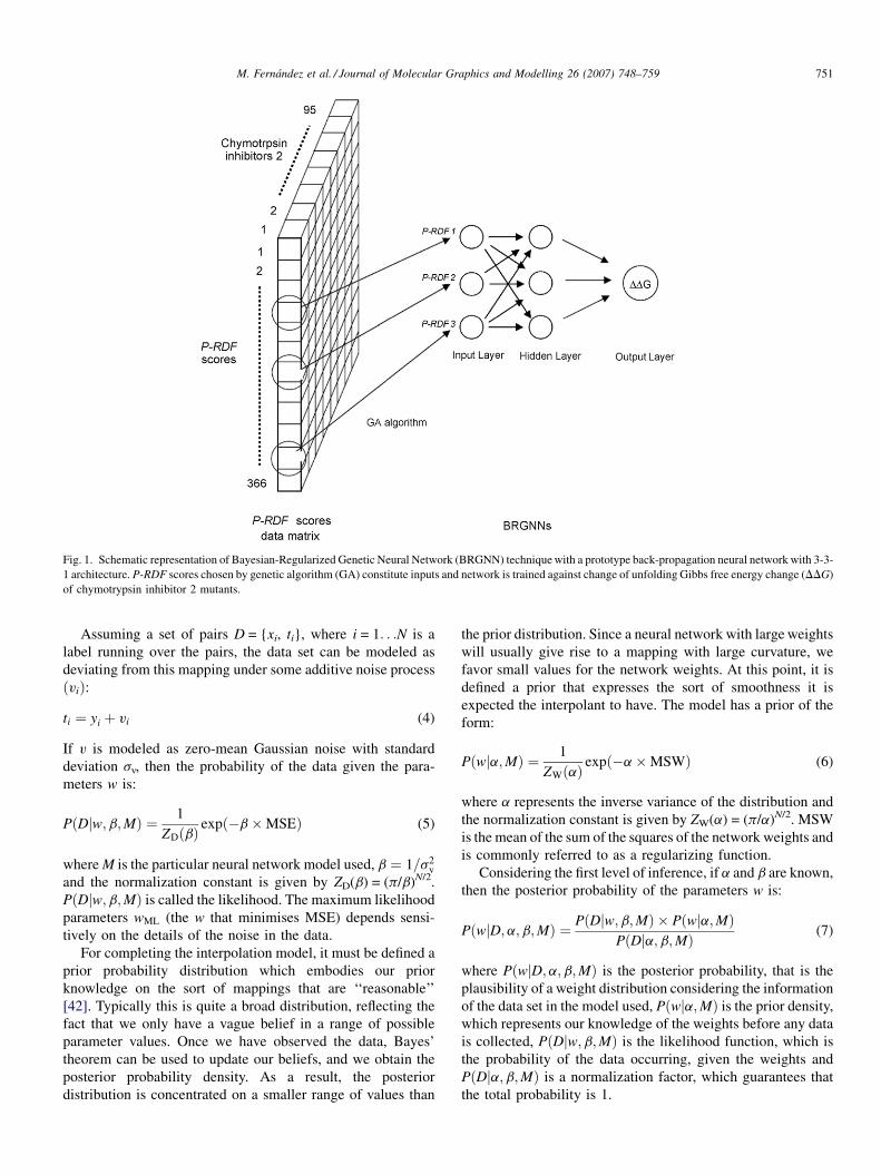
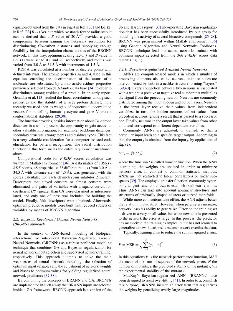
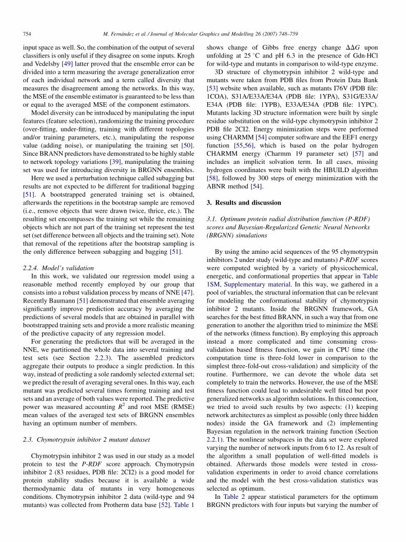
Fig. 1. Schematic representation of Bayesian-Regularized Genetic Neural Network (BRGNN) technique with a prototype back-propagation neural network with 3-3-
1 architecture. P-RDF scores chosen by genetic algorithm (GA) constitute inputs and network is trained against change of unfolding Gibbs free energy change (DDG)
of chymotrypsin inhibitor 2 mutants.
M. Fernandez et al. / Journal of Molecular Graphics and Modelling 26 (2007) 748–759 751
Assuming a set of pairs D = {xi, ti}, where i = 1. . .N is a
label running over the pairs, the data set can be modeled as
deviating from this mapping under some additive noise process
ðviÞ:
ti ¼ yi þ vi (4)
If v is modeled as zero-mean Gaussian noise with standard
deviation sv, then the probability of the data given the para-
meters w is:
PðDjw;b;MÞ ¼ 1
ZDðbÞexpð�b�MSEÞ (5)
where M is the particular neural network model used, b ¼ 1=s2v
and the normalization constant is given by ZD(b) = (p/b)N/2.
PðDjw;b;MÞ is called the likelihood. The maximum likelihood
parameters wML (the w that minimises MSE) depends sensi-
tively on the details of the noise in the data.
For completing the interpolation model, it must be defined a
prior probability distribution which embodies our prior
knowledge on the sort of mappings that are ‘‘reasonable’’
[42]. Typically this is quite a broad distribution, reflecting the
fact that we only have a vague belief in a range of possible
parameter values. Once we have observed the data, Bayes’
theorem can be used to update our beliefs, and we obtain the
posterior probability density. As a result, the posterior
distribution is concentrated on a smaller range of values than
the prior distribution. Since a neural network with large weights
will usually give rise to a mapping with large curvature, we
favor small values for the network weights. At this point, it is
defined a prior that expresses the sort of smoothness it is
expected the interpolant to have. The model has a prior of the
form:
Pðwja;MÞ ¼ 1
ZWðaÞexpð�a�MSWÞ (6)
where a represents the inverse variance of the distribution and
the normalization constant is given by ZW(a) = (p/a)N/2. MSW
is the mean of the sum of the squares of the network weights and
is commonly referred to as a regularizing function.
Considering the first level of inference, if a and b are known,
then the posterior probability of the parameters w is:
PðwjD;a;b;MÞ ¼ PðDjw;b;MÞ � Pðwja;MÞPðDja;b;MÞ (7)
where PðwjD;a;b;MÞ is the posterior probability, that is the
plausibility of a weight distribution considering the information
of the data set in the model used, Pðwja;MÞ is the prior density,
which represents our knowledge of the weights before any data
is collected, PðDjw;b;MÞ is the likelihood function, which is
the probability of the data occurring, given the weights and
PðDja;b;MÞ is a normalization factor, which guarantees that
the total probability is 1.
M. Fernandez et al. / Journal of Molecular Graphics and Modelling 26 (2007) 748–759752
Considering that the noise in the training set data is Gaussian
and that the prior distribution for the weights is Gaussian, the
posterior probability fulfills the relation:
PðwjD;a;b;MÞ ¼ 1
ZF
expð�FÞ (8)
where ZF depends of objective function parameters. So under
this framework, minimization of F is identical to find the
(locally) most probable parameters [41].
In short, Bayesian regularization involves modifying the
performance function (F) defined in Eq. (3). This equation can
be generalized (and improved) by adding an additional term.
F ¼ b�MSEþ a�MSW (9)
The relative size of the objective function parameters a and b
dictates the emphasis for getting a smoother network response.
MacKay’s Bayesian framework automatically adapts the reg-
ularization parameters to maximize the evidence of the training
data [41].
Bayesian regularization overcomes the remaining deficien-
cies of neural networks and produces predictors that are robust
and well matched to the data; in this sense, BRANNs have been
successfully applied in structure–property/activity analysis
[25–30].
Fully connected, three-layer BRANNs with back-propaga-
tion training were implemented in MATLAB environment [36].
In these nets, the transfer functions of input and output layers
were linear, and the hidden layer had neurons with a hyperbolic
tangent transfer function. Inputs and targets took the values
from independent variables selected by the GA and DDG
values, respectively; both were normalized prior to network
training. BRANN training was carried out according to the
Levenberg–Marquardt optimization [43]. The initial value for
m (the scalar controlling both the magnitude and direction of
the search direction in the Levenberg–Marquardt optimization)
was 0.005 with decrease and increase factors of 0.1 and 10,
respectively. The training was stopped when m became larger
than 1010.
2.2.2. Genetic algorithm
GAs are governed by biological evolution rules [44]. They
are stochastic optimization methods that have been inspired by
evolutionary principles. The distinctive aspect of a GA is that it
investigates many possible solutions simultaneously, each of
which explores different regions in parameter space [45]. The
first step is to create a population of N individuals. Each
individual encodes the same number of randomly chosen
descriptors. The fitness of each individual in this generation is
determined. In the second step, a fraction of children of the next
generation is produced by crossover (crossover children) and
the rest by mutation (mutation children) from the parents on the
basis of their scaled fitness scores. The new offspring contains
characteristics from two or one of its parents.
In the BRGNN approach, individuals in the populations are
BRANN predictors with a fixed architecture and the MSE of data
fitting was tried as the individual fitness function. An individual is
represented by a string of integers which means the numbering of
the rows in the descriptors matrix (366 rows � 95 columns) that
will be tested as BRANN inputs. So and Karplus [37], used a
variety of fitness functions which are proportional to the residual
error of the training set, the test set, or even the cross-validation
set from the neural network simulations. However, since we
implemented regularized networks, we tried the MSE of data
fitting as the individual fitness function. The first step is to create a
gene pool (population of neural network predictors) of N
individuals. Each individual encodes the same number of
descriptors; the descriptors are randomly chosen from a common
data matrix, and in a way such that (1) no two individuals can
have exactly the same set of descriptors and (2) all descriptors in a
given individual must be different. The fitness of each individual
in this generation is determined by the MSE of the model and
scaled using and scaling function. A top scaling fitness function
scaled a top fraction of the individuals in a population equally;
these individuals have the same probability to be reproduced
while the rest are assigned the value 0.
The next step, a fraction of children of the next generation is
produced by crossover (crossover children) and the rest by
mutation (mutation children) from the parents. Sexual and
asexual reproductions take place so that the new offspring
contains characteristics from two or one of its parents. In a
sexual reproduction two individuals are selected probabilisti-
cally on the basis of their scaled fitness scores and serve as
parents. Next, in a crossover each parent contributes a random
selection of half of its descriptor set and a child is constructed
by combining these two halves of ‘‘genetic code’’. Finally, the
rest of the individuals in the new generation are obtained by
asexual reproduction when parents selected randomly are
subjected to a random mutation in one of its genes, i.e., one
descriptor is replaced by another.
Similarly to So and Karplus [37], we also included elitism
which protects the fittest individual in any given generation
from crossover or mutation during reproduction. The genetic
content of this individual simply moves on to the next
generation intact. This selection, crossover and mutation
process is repeated until all of the N parents in the population
are replaced by their children. The fitness score of each member
of this new generation is again evaluated, and the reproductive
cycle is continued until a 90% of the generations showed the
same target fitness score [46].
Differently to other GA-based approach, the objective of our
algorithm is not to obtain a sole optimum model but a reduced
population of well-fitted models, with MSE lower than a
threshold MSE value, at which the Bayesian regularization
guaranties network to posses good generalization abilities [47].
This is because we used MSE of data training fitting instead of
cross-validation or test set MSE values as cost function and
therefore the optimum model cannot be directly derived from
the best-fitted model yielded by the genetic search. However,
from cross-validation experiments over the subpopulation of
well-fitted models it can derive the best generalizable network
with the highest predictive power. This process also assures to
avoid chance correlations. This approach have shown to be
highly efficient in comparison with cross-validation-based
GA approach since only optimum models, according to the
M. Fernandez et al. / Journal of Molecular Graphics and Modelling 26 (2007) 748–759 753
Bayesian regularization, are cross-validated at the end of the
routine and not all the model generated throughout all the
search process [47].
2.2.3. Artificial neural network ensembles
Artificial neural network ensemble (NNE) is a learning
paradigm where many ANNs are jointly used to solve a
Table 1
Experimental and calculated change of unfolding Gibbs free energy change (DDGa) a
according to a 50 members neural network ensemble of optimum model BRGNN
Mutant DDG (kcal/mol)
Exp. Cal.trainb Cal.test
c
Wild 0.00 �0.38 �0.41
A35G �1.09 �1.53 �1.85
A77G �1.88 �1.21 �0.70
D42A �0.96 �1.39 �1.40
D64A �0.80 �0.50 �0.48
D71A �3.41 �2.14 �1.25
E26A �0.47 �0.70 �0.74
E26Q �0.62 �0.43 �0.38
E33A/E34A �0.76 �0.97 �1.81
E33D �0.52 �0.61 �0.60
E33N �0.70 �0.83 �0.79
E33Q �0.29 �0.57 �0.61
E34D �0.74 �0.68 �0.54
E34N �1.07 �0.73 �0.77
E34Q �0.47 �0.63 �0.61
E45A �0.32 �0.58 �0.61
E60A �0.68 �0.38 �0.35
F69A �3.84 �3.24 �3.17
F69L �2.11 �2.07 �2.11
F69V �2.39 �1.99 �1.98
I39V �1.27 �1.39 �1.44
I48A �3.84 �3.64 �3.51
I48A/I76V �4.05 �4.24 �4.74
I48V �1.09 �1.00 �1.05
I49A �2.12 �3.14 �3.39
I49G �3.52 �3.67 �4.05
I49T �1.34 �1.67 �1.78
I49V 0.08 �1.10 �1.13
I56A �0.03 �0.65 �0.69
I76A �4.25 �3.51 �2.95
I76V 0.21 0.25 0.53
K21A �0.55 �0.69 �0.69
K21A/E26A �1.10 �1.32 �1.48
K21M �0.67 �0.30 �0.24
K30A 0.42 0.05 �0.15
K36A �0.49 �0.52 �0.60
K36G �2.32 �2.31 �2.36
K37A 0.21 �0.49 �0.53
K37G �0.99 �1.20 �1.22
K43A �0.65 �1.24 �1.56
K43G �3.19 �3.19 �3.05
K72N 0.00 �1.05 �1.18
L27A �2.64 �1.20 �1.01
L40A �1.33 �1.04 �0.97
L40G �1.38 �1.35 �1.39
L51A �2.37 �1.86 �1.76
L51A/F69L �3.42 �3.77 �3.98
L51A/V57A �3.16 �3.28 �3.38
a DDG negative and positive values mean destabilizing and stabilizing mutationb Calculated as average over training sets using a 50 members ensemble.c Calculated as average over test sets in the using a 50 members ensemble.
problem. On the basis of this judgement, a collection of a finite
number of neural networks is trained for the same task and the
outputs can be combined to form one unified prediction. As a
result, the generalization ability of the neural network system
can be significantly improved [48].
An effective NNE should consist of a set of ANNs that are
not highly correct and make their errors on different parts of the
t 25 8C, pH 6.3 in Gdn�HCl for chymotrypsin inhibitor 2 wild-type and mutants
2
Mutant DDG (kcal/mol)
Exp. Cal.trainb Cal.test
c
L51A/V57/AF69L �3.48 �3.53 �4.64
L51I �0.26 �0.64 �1.34
L51V �0.50 �0.68 �0.76
L51V/F69L �2.42 �1.99 �1.90
L51V/V57A �1.85 �1.36 �1.19
L51V/V57A/F69L �2.72 �3.23 �3.34
L68A �3.82 �3.59 �3.46
N75A �0.83 �1.07 �1.61
N75D �1.21 �0.55 �0.18
P25A �1.57 �0.91 �0.60
P25A/A35G �2.65 �2.54 �2.33
P44A �1.76 �1.73 �1.71
P52A �0.17 �1.02 �1.47
P80A �3.34 �3.50 �4.12
Q41A �0.02 �0.36 �0.43
Q41G �0.60 �0.41 �0.37
R62A �0.58 �0.61 �0.66
R62A/D64A �1.22 �1.15 �1.08
S31A �0.89 �0.38 �0.41
S31A/E33A/E34A �1.67 �1.52 �0.41
S31G �0.80 �0.51 �0.47
S31G/E33A/E34A �1.63 �1.56 �1.03
T22A �0.85 �1.18 �1.08
T22G �1.16 �1.52 �1.57
T22V �0.32 �0.20 �0.18
T55A 0.23 �0.40 �0.46
T55S �0.02 �0.41 �0.47
T55V �0.76 �0.18 �0.09
T58A �0.69 �0.41 �0.39
T58A/E60A �0.87 �0.39 �0.37
T58D 0.04 �0.39 �0.43
T58D/E60A �0.25 �0.36 �0.41
V38A �0.46 �1.20 �1.25
V53A �0.64 �1.21 �1.27
V53G �2.43 �1.89 �1.74
V53T �1.03 �0.51 �0.49
V57A �1.47 �1.18 �1.20
V57A/F69L �2.58 �3.16 �3.62
V57A/V79A �4.37 �3.64 �3.43
V66A �4.88 �3.44 �2.92
V70A �1.95 �1.55 �1.44
V79A �1.51 �2.26 �2.53
V79G �3.24 �3.22 �3.24
V79T �0.38 �0.84 �1.18
V82A �1.45 �1.69 �1.80
V82G �3.50 �3.09 �2.89
V82T �1.15 �0.71 �0.70
s, respectively.
M. Fernandez et al. / Journal of Molecular Graphics and Modelling 26 (2007) 748–759754
input space as well. So, the combination of the output of several
classifiers is only useful if they disagree on some inputs. Krogh
and Vedelsby [49] latter proved that the ensemble error can be
divided into a term measuring the average generalization error
of each individual network and a term called diversity that
measures the disagreement among the networks. In this way,
the MSE of the ensemble estimator is guaranteed to be less than
or equal to the averaged MSE of the component estimators.
Model diversity can be introduced by manipulating the input
features (feature selection), randomizing the training procedure
(over-fitting, under-fitting, training with different topologies
and/or training parameters, etc.), manipulating the response
value (adding noise), or manipulating the training set [50].
Since BRANN predictors have demonstrated to be highly stable
to network topology variations [39], manipulating the training
set was used for introducing diversity in BRGNN ensembles.
Here we used a perturbation technique called subagging but
results are not expected to be different for traditional bagging
[51]. A bootstrapped generated training set is obtained,
afterwards the repetitions in the bootstrap sample are removed
(i.e., remove objects that were drawn twice, thrice, etc.). The
resulting set encompasses the training set while the remaining
objects which are not part of the training set represent the test
set (set difference between all objects and the training set). Note
that removal of the repetitions after the bootstrap sampling is
the only difference between subagging and bagging [51].
2.2.4. Model’s validation
In this work, we validated our regression model using a
reasonable method recently employed by our group that
consists into a robust validation process by means of NNE [47].
Recently Baumann [51] demonstrated that ensemble averaging
significantly improve prediction accuracy by averaging the
predictions of several models that are obtained in parallel with
bootstrapped training sets and provide a more realistic meaning
of the predictive capacity of any regression model.
For generating the predictors that will be averaged in the
NNE, we partitioned the whole data into several training and
test sets (see Section 2.2.3). The assembled predictors
aggregate their outputs to produce a single prediction. In this
way, instead of predicting a sole randomly selected external set;
we predict the result of averaging several ones. In this way, each
mutant was predicted several times forming training and test
sets and an average of both values were reported. The predictive
power was measured accounting R2 and root MSE (RMSE)
mean values of the averaged test sets of BRGNN ensembles
having an optimum number of members.
2.3. Chymotrypsin inhibitor 2 mutant dataset
Chymotrypsin inhibitor 2 was used in our study as a model
protein to test the P-RDF score approach. Chymotrypsin
inhibitor 2 (83 residues, PDB file: 2CI2) is a good model for
protein stability studies because it is available a wide
thermodynamic data of mutants in very homogeneous
conditions. Chymotrypsin inhibitor 2 data (wild-type and 94
mutants) was collected from Protherm data base [52]. Table 1
shows change of Gibbs free energy change DDG upon
unfolding at 25 8C and pH 6.3 in the presence of Gdn�HCl
for wild-type and mutants in comparison to wild-type enzyme.
3D structure of chymotrypsin inhibitor 2 wild-type and
mutants were taken from PDB files from Protein Data Bank
[53] website when available, such as mutants I76V (PDB file:
1COA), S31A/E33A/E34A (PDB file: 1YPA), S31G/E33A/
E34A (PDB file: 1YPB), E33A/E34A (PDB file: 1YPC).
Mutants lacking 3D structure information were built by single
residue substitution on the wild-type chymotrypsin inhibitor 2
PDB file 2CI2. Energy minimization steps were performed
using CHARMM [54] computer software and the EEF1 energy
function [55,56], which is based on the polar hydrogen
CHARMM energy (Charmm 19 parameter set) [57] and
includes an implicit solvation term. In all cases, missing
hydrogen coordinates were built with the HBUILD algorithm
[58], followed by 300 steps of energy minimization with the
ABNR method [54].
3. Results and discussion
3.1. Optimum protein radial distribution function (P-RDF)
scores and Bayesian-Regularized Genetic Neural Networks
(BRGNN) simulations
By using the amino acid sequences of the 95 chymotrypsin
inhibitors 2 under study (wild-type and mutants) P-RDF scores
were computed weighted by a variety of physicochemical,
energetic, and conformational properties that appear in Table
1SM, Supplementary material. In this way, we gathered in a
pool of variables, the structural information that can be relevant
for modeling the conformational stability of chymotrypsin
inhibitor 2 mutants. Inside the BRGNN framework, GA
searches for the best fitted BRANN, in such a way that from one
generation to another the algorithm tried to minimize the MSE
of the networks (fitness function). By employing this approach
instead a more complicated and time consuming cross-
validation based fitness function, we gain in CPU time (the
computation time is three-fold lower in comparison to the
simplest three-fold-out cross-validation) and simplicity of the
routine. Furthermore, we can devote the whole data set
completely to train the networks. However, the use of the MSE
fitness function could lead to undesirable well fitted but poor
generalized networks as algorithm solutions. In this connection,
we tried to avoid such results by two aspects: (1) keeping
network architectures as simplest as possible (only three hidden
nodes) inside the GA framework and (2) implementing
Bayesian regulation in the network training function (Section
2.2.1). The nonlinear subspaces in the data set were explored
varying the number of network inputs from 6 to 12. As result of
the algorithm a small population of well-fitted models is
obtained. Afterwards those models were tested in cross-
validation experiments in order to avoid chance correlations
and the model with the best cross-validation statistics was
selected as optimum.
In Table 2 appear statistical parameters for the optimum
BRGNN predictors with four inputs but varying the number of
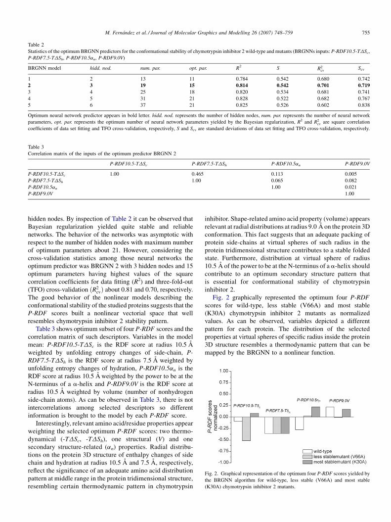
Fig. 2. Graphical representation of the optimum four P-RDF scores yielded by
the BRGNN algorithm for wild-type, less stable (V66A) and most stable
(K30A) chymotrypsin inhibitor 2 mutants.
Table 2
Statistics of the optimum BRGNN predictors for the conformational stability of chymotrypsin inhibitor 2 wild-type and mutants (BRGNNs inputs: P-RDF10.5-TDSc,
P-RDF7.5-TDSh, P-RDF10.5an, P-RDF9.0V)
BRGNN model hidd. nod. num. par. opt. par. R2 S R2cv
Scv
1 2 13 11 0.784 0.542 0.680 0.742
2 3 19 15 0.814 0.542 0.701 0.7193 4 25 18 0.820 0.534 0.681 0.741
4 5 31 21 0.828 0.522 0.682 0.767
5 6 37 21 0.825 0.526 0.602 0.838
Optimum neural network predictor appears in bold letter. hidd. nod. represents the number of hidden nodes, num. par. represents the number of neural network
parameters, opt. par. represents the optimum number of neural network parameters yielded by the Bayesian regularization, R2 and R2cv are square correlation
coefficients of data set fitting and TFO cross-validation, respectively, S and Scv are standard deviations of data set fitting and TFO cross-validation, respectively.
Table 3
Correlation matrix of the inputs of the optimum predictor BRGNN 2
P-RDF10.5-TDSc P-RDF7.5-TDSh P-RDF10.5an P-RDF9.0V
P-RDF10.5-TDSc 1.00 0.465 0.113 0.005
P-RDF7.5-TDSh 1.00 0.065 0.082
P-RDF10.5an 1.00 0.021
P-RDF9.0V 1.00
M. Fernandez et al. / Journal of Molecular Graphics and Modelling 26 (2007) 748–759 755
hidden nodes. By inspection of Table 2 it can be observed that
Bayesian regularization yielded quite stable and reliable
networks. The behavior of the networks was asymptotic with
respect to the number of hidden nodes with maximum number
of optimum parameters about 21. However, considering the
cross-validation statistics among those neural networks the
optimum predictor was BRGNN 2 with 3 hidden nodes and 15
optimum parameters having highest values of the square
correlation coefficients for data fitting (R2) and three-fold-out
(TFO) cross-validation ðR2cvÞ about 0.81 and 0.70, respectively.
The good behavior of the nonlinear models describing the
conformational stability of the studied proteins suggests that the
P-RDF scores built a nonlinear vectorial space that well
resembles chymotrypsin inhibitor 2 stability pattern.
Table 3 shows optimum subset of four P-RDF scores and the
correlation matrix of such descriptors. Variables in the model
mean: P-RDF10.5-TDSc is the RDF score at radius 10.5 A
weighted by unfolding entropy changes of side-chain, P-
RDF7.5-TDSh is the RDF score at radius 7.5 A weighted by
unfolding entropy changes of hydration, P-RDF10.5an is the
RDF score at radius 10.5 A weighted by the power to be at the
N-terminus of a a-helix and P-RDF9.0V is the RDF score at
radius 10.5 A weighted by volume (number of nonhydrogen
side-chain atoms). As can be observed in Table 3, there is not
intercorrelations among selected descriptors so different
information is brought to the model by each P-RDF score.
Interestingly, relevant amino acid/residue properties appear
weighting the selected optimum P-RDF scores: two thermo-
dynamical (-TDSc, -TDSh), one structural (V) and one
secondary structure-related (an) properties. Radial distribu-
tions on the protein 3D structure of enthalpy changes of side
chain and hydration at radius 10.5 A and 7.5 A, respectively,
reflect the significance of an adequate amino acid distribution
pattern at middle range in the protein tridimensional structure,
resembling certain thermodynamic pattern in chymotrypsin
inhibitor. Shape-related amino acid property (volume) appears
relevant at radial distributions at radius 9.0 A on the protein 3D
conformation. This fact suggests that an adequate packing of
protein side-chains at virtual spheres of such radius in the
protein tridimensional structure contributes to a stable folded
state. Furthermore, distribution at virtual sphere of radius
10.5 A of the power to be at the N-terminus of a a-helix should
contribute to an optimum secondary structure pattern that
is essential for conformational stability of chymotrypsin
inhibitor 2.
Fig. 2 graphically represented the optimum four P-RDF
scores for wild-type, less stable (V66A) and most stable
(K30A) chymotrypsin inhibitor 2 mutants as normalized
values. As can be observed, variables depicted a different
pattern for each protein. The distribution of the selected
properties at virtual spheres of specific radius inside the protein
3D structure resembles a thermodynamic pattern that can be
mapped by the BRGNN to a nonlinear function.
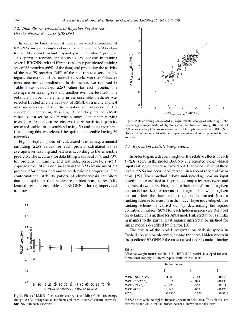
Fig. 4. Plots of average calculated vs. experimental change of unfolding Gibbs
free energy change (DDG) of chymotrypsin inhibitor 2 in training (*) and test
(*) sets according to 50 member ensemble of the optimum network BRGNN 2.
Dotted line are an ideal fit with the respective intercept and slope equal to zero
and one.
M. Fernandez et al. / Journal of Molecular Graphics and Modelling 26 (2007) 748–759756
3.2. Data-diverse ensembles of Bayesian-Regularized
Genetic Neural Networks (BRGNN)
In order to build a robust model we used ensembles of
BRGNNs instead a single network to calculate the DDG values
for wild-type and mutant chymotrypsin inhibitor 2 proteins.
This approach recently applied by us [25] consists in training
several BRGNNs with different randomly partitioned training
sets of 66 proteins (66% of the data) and predicting the activity
of the rest 29 proteins (34% of the data) in test sets. In this
regard, the outputs of the trained networks were combined to
form one unified prediction. In this sense, we reported in
Table 1 two calculated DDG values for each protein: one
average over training sets and another over the test sets. The
optimum number of elements in the ensemble predictor was
selected by studying the behavior of RMSE of training and test
sets respectively versus the number of networks in the
ensemble. Concerning this, Fig. 3 depicts plots of RMSE
values of test set for NNEs with number of members varying
from 2 to 75. As can be observed such statistical quantity
remained stable for ensembles having 50 and more members.
Considering this, we selected the optimum ensemble having 50
networks.
Fig. 4 depicts plots of calculated versus experimental
unfolding DDG values for each protein calculated as an
average over training and test sets according to the ensemble
predictor. The accuracy for data fitting was about 84% and 70%
for proteins in training and test sets, respectively. P-RDF
approach well fit in a nonlinear way the DDG by means of 3D
protein information and amino acid/residues properties. The
conformational stability pattern of chymotrypsin inhibitors
that the optimum four scores resembled was successfully
learned by the ensemble of BRGNNs during supervised
training.
Fig. 3. Plots of RMSE of test set for change of unfolding Gibbs free energy
change (DDG) average values for 20 ensembles vs. number of neural networks
BRGNN 2 in each ensemble.
3.3. Regression model’s interpretation
In order to gain a deeper insight on the relative effects of each
P-RDF score in the model BRGNN 2, a reported weight-based
input ranking scheme was carried out. Black-box nature of three
layers ANNs has been ‘‘deciphered’’ in a recent report of Guha
et al. [59]. Their method allows understanding how an input
descriptor is correlated to the predicted output by the network and
consists of two parts. First, the nonlinear transform for a given
neuron is linearized. Afterward, the magnitude in which a given
neuron affects the downstream output is determined. Next, a
ranking scheme for neurons in the hidden layer is developed. The
ranking scheme is carried out by determining the square
contribution values (SCV) for each hidden neuron (see Ref. [59]
for details). This method for ANN model interpretation is similar
in manner to the partial least squares interpretation method for
linear models described by Stanton [60].
The results of the model interpretation analysis appear in
Table 4. As can be observed, among the three hidden nodes in
the predictor BRGNN 2 the most ranked node is node 1 having
Table 4
Effective weight matrix for the 4-3-1 BRGNN 2 model developed for con-
formational stability of chymotrypsin inhibitor 2 mutants
Hidden nodes
1 3 2
P-RDF10.5-TDSc 4.081 �2.142 �0.010P-RDF7.5-TDSh 1.519 �0.014 �0.436
P-RDF10.5Dn �1.927 0.560 0.611
P-RDF9.0V 1.362 0.977 �0.475
SCVs 0.7826 0.2173 0.0001
P-RDF score with the highest impacts appears in bold letter. The columns are
ordered by the SCVs for the hidden neurons, shown in the last row.
M. Fernandez et al. / Journal of Molecular Graphics and Modelling 26 (2007) 748–759 757
a SCV value about 0.78, which is 3.6-fold higher than hidden
node 3 whilst node 2 is practically irrelevant. According to the
Guha’s analysis [59] the most ranked node has the major impact
in the overall output of the neural network. Consequently, the
most weighted inputs in such node represent the most relevant
descriptors for the regression problem under study. Specifically
in Table 4, all descriptors have weights > j1j on the most
ranked node. However, descriptor P-RDF10.5-TDSc, which
represents spherical distribution at radius 10.5 A of entropy
change of side-chains on the 3D structure of chymotrypsin
inhibitor 2 mutants, exhibits the highest relevance in
comparison to the other descriptors. This result well agrees
with reports regarding point mutations in proteins that state that
modification of entropy of 3D structure of proteins affects the
conformational stability [13,61].
It is noticeable that -TDSh property also appeared relevant
when we modeled the conformational stability of human
lysozyme but exploiting only sequence information by using
AASA vectors [29]. We can state that occurrence in the model of
hydrophobicity-related property (-TDSh) is in concordance
with thermal denaturation mechanism hypothesis. For thermal
denaturation process of globular proteins, Privalov and Gill [62]
stated that hydration equilibrium at high temperatures, polar
interactions between solvent and polar residues in the protein, is
the main cause of unfolding meanwhile hydrophobic interac-
tions contributes to keep the folded state.
Otherwise, the volume available to a side-chain at protein
interior can produce energetic penalty for conformational
alterations after mutation [63], this effect is highly influenced
by the size (V) of the substitute, added and also surrounding
residues. Mutations may cause an unfavorable packing energy
due to the rigidity of surrounding residues or, alternatively, the
substituting residues themselves may be forced into unfavor-
able rotational isomers. Similarly, some surroundings of
mutation positions may be readily deformable or there may
be compensating effects that yield no net packing energy
change [63]. This property (V) also appeared weighting
optimum AASA vectors used for modeling the conformational
stability of gene V protein in a previous work [30].
On the other hand, the high relevance of the power to be at
the N-terminus of a a-helix strongly suggested that optimum
secondary structure pattern is another key factor for a stable
tertiary conformation. Point mutations studies have highlighted
the role of secondary structure propensities in protein stability.
Manipulating favorable and unfavorable secondary structure
propensities at certain positions in a protein can produce
significant variations in protein stability [12]. Furthermore,
secondary structure propensities has been also previously
selected inside the BRGNN algorithm as optimum weighting
parameters for modeling the conformational stability of human
lysozyme [29] and gene V protein [30] in two previous works.
The predicted power of our ensemble model is in the range
of the report of Marrero-Ponce et al. [21] in which they
extended topological indexes to the study of biological
macromolecules. In such report, protein linear indices of the
‘macromolecular pseudograph Ca-atom adjacency matrix’
were applied to the prediction of actual melting points of Arc
repressor mutants and a linear model was obtained using
multilinear equation that described about 72% of cross-
validation data variance. However, it most be taken into account
that conformational stability is a more complex protein
property in comparison to other physical stability measure-
ments, such as protein melting point. In this sense, the accuracy
over 70% of our approach for predicting actual DDG values of
chymotrypsin inhibitor 2 mutants is remarkably good.
Concerning the prediction of Gibbs free energy change of
proteins, our approach is more accurate than previous reports in
which no more than 60% of validation data variance was
described; although such models used larger and more varied
datasets (>1000) [12,16,19,61,64]. P-RDF scores were able of
resembling a 3D amino acid interaction pattern in chymo-
trypsin inhibitor 2 that was successfully learned by BRGNNs.
At the moment, the prediction approach presented here is
protein-specific and then one needs to obtain a model for each
protein of interest. We gain in quality of predictions in
comparison to more comprehensive models mentioned above
but with lower generalization abilities. It is noteworthy that our
predictor, differently to the most of the reported approaches,
successfully encompasses single, double and any number point
mutants. The aim of our work was just to present a reliable
predictor for the conformational stability of a sole protein using
3D structure-derived information and a wide thermodynamic
data of their mutants.
In order to compute P-RDF scores we used experimental X-
ray structural information of the chymotrypsin inhibitor 2
mutants when available or, similarly to Gonzalez-Dıaz and
coworkers [20], we built the mutants in silico by simple residue
substitution following by energy minimization. We must clearly
stay that generating the 3D structure of a protein mutant by
simple in silico substitution of one residue by another is a rough
approximation to the mutant structure, even using energy
minimization. However, it is adequate for considering some 3D
information in the neural network simulations instead to strictly
use the scarce information derived from the sequence. In this
connection, when comparing our results using P-RDF scores to
previous studies of our group using AASAvectors [29,30] derived
from the protein primary sequence it is found that prediction
accuracy was now increased up to 0.7. Similar accuracy over 0.7
was observed when using autocorrelation vectors calculated over
the protein 3D structures instead sequences for solving the same
problem, the conformational stability of chymotrypsin inhibitor
2 mutants [65]. Despite the disadvantage of some previous
thermodynamic experimental data is required for generating a
training set, our modeling technique is a viable alternative for
stability prediction when some thermodynamic data exits.
4. Conclusions
Protein structures are stabilized by numerous intramolecular
interactions such as hydrophobic, electrostatic, van der Waals
and hydrogen-bond. Due to the availability of an enormous
amount of thermodynamic data on protein stability it is possible
to use structure–properties relationship approach for protein
modeling. We extended the concept of RDF scores in molecules
M. Fernandez et al. / Journal of Molecular Graphics and Modelling 26 (2007) 748–759758
to the 3D structure of proteins as a tool for encoding protein
structural information for supervised training of ANNs. In this
sense, novel Protein radial distribution function (P-RDF) scores
were obtained by calculating RDF at different radius on the
protein 3D structure weighted by 48 amino acid/residue
properties selected from the AAindex data base. BRGNNs
showed again to be a powerful technique for feature selection and
mathematical modeling. This approach yielded a reliable and
robust four-input ensemble model for the conformational
stability of chymotrypsin inhibitor 2 mutants that describes
about 85% and 70% of training and test set variances. The present
work demonstrates the successful application of the P-RDF
scores to the modeling of protein conformational stability in
combination with BRGNN approach. Encoding amino acid
properties and protein 3D structure information on a same pool of
descriptors are more appropriate than other approaches
considering only amino acid substitution information and partial
3D proximity to the substitution site. P-RDF also overcomes
some previous results using only sequence-derived information.
This approach leads to a powerful method for the scientific
community interested in protein prediction studies. Despite of
one model per protein is required according to the approach
present here, a general model encompassing a large and varied
mutant data (>1000) as well as protein-specific models for other
proteins are under development by our group at the present time.
Acknowledgements
Authors would like to acknowledge to the anonymous
referees for theirs useful comments that helped to improve the
quality of the manuscript. Financial supports of this research by
Cuban Ministerio de Ciencia, Tecnologıa y Medio Ambiente
(CITMA) through a grant to M. Fernandez (Grant No.
20104102).
Appendix A. Supplementary data
Supplementary data associated with this article can be found,
in the online version, at doi:10.1016/j.jmgm.2007.04.011.
References
[1] J. Saven, Combinatorial protein design, Curr. Opin. Struct. Biol. 12 (2002)
453–458.
[2] J. Mendes, R. Guerois, L. Serrano, Energy estimation in protein design,
Curr. Opin. Struct. Biol. 12 (2002) 441–446.
[3] D.N. Bolon, J.S. Marcus, S.A. Ross, S.L. Mayo, Prudent modeling of core
polar residues in computational protein design, J. Mol. Biol. 329 (2003)
611–622.
[4] L.L. Looger, M.A. Dwyer, J.J. Smith, H.W. Helling, Computational design
of receptor and sensor proteins with novel functions, Nature 423 (2003)
185–190.
[5] L.X. Dang, K.M. Merz, P.A. Kollman, Free-energy calculations on protein
stability: Thr-1573Val-157 mutation of T4 lysozyme, J. Am. Chem. Soc.
111 (1989) 8505–8508.
[6] T. Lazaridis, M. Karplus, Effective energy functions for protein structure
prediction, Curr. Opin. Struct. Biol. 10 (2000) 139–145.
[7] C. Lee, M. Levitt, Accurate prediction of the stability and activity effects of
site-directed mutagenesis on a protein core, Nature 352 (1991) 448–451.
[8] C. Lee, Testing homology modeling on mutant proteins: predicting
structural and thermodynamic effects in the Ala98-Val mutants of T4
lysozyme, Fold. Des. 1 (1995) 1–12.
[9] C.M. Topham, N. Srinivasan, T.L. Blundell, Prediction of the stability of
protein mutants based on structural environment-dependent amino acid
substitution and propensity tables, Protein Eng. 10 (1997) 7–21.
[10] D. Gilis, M. Rooman, Prediction of stability changes upon single site
mutations using database-derived potentials, Theor. Chem. Acc. 101
(1999) 46–50.
[11] (a) E. Lacroix, A.R. Viguera, L. Serrano, Elucidating the folding problem of
alpha-helices: local motifs, long-range electrostatics, ionic-strength depen-
dence and prediction of NMR parameters, J. Mol. Biol. 284 (1998) 173–191;
(b) V. Munoz, L. Serrano, Development of the multiple sequence approx-
imation within the AGADIR model of alpha-helix formation: comparison
with Zimm–Bragg and Lifson–Roig formalisms, Biopolymers 41 (1997)
495–509.
[12] R. Guerois, J.E. Nielsen, L. Serrano, Predicting changes in the stability of
proteins and protein complexes: a study of more than 1000 mutations, J.
Mol. Biol. 320 (2002) 369–387.
[13] M.M. Gromiha, M. Oobatake, H. Kono, H. Uedaira, A. Sarai, Relationship
between amino acid properties and protein stability: buried mutations, J.
Protein Chem. 18 (1999) 565–578.
[14] M.M. Gromiha, M. Oobatake, H. Kono, H. Uedaira, A. Sarai, Role of
structural and sequence information in the prediction of protein stability
changes: comparison between buried and partially buried mutations,
Protein Eng. 12 (1999) 549–555.
[15] M.M. Gromiha, M. Oobatake, H. Kono, H. Uedaira, A. Sarai, Importance
of surrounding residues for protein stability of partially buried mutations,
J. Biomol. Struct. Dyn. 18 (2000) 1–16.
[16] H. Zhou, Y. Zhou, Stability scale and atomic solvation parameters
extracted from 1023 mutation experiment, Proteins 49 (2002) 483–492.
[17] S. Levin, B.H. Satir, POLINA: Detection and evaluation of single amino acid
substitutions in protein superfamilies, Bioinformatics 14 (1998) 374–375.
[18] C.M. Frenz, Neural network-based prediction of mutation-induced protein
stability changes in staphylococcal nuclease at 20 residue positions,
Proteins 59 (2005) 147–151.
[19] (a) E. Capriotti, P. Fariselli, R. Casadio, A neural-network-based method
for predicting protein stability changes upon single mutations, Bioinfor-
matics 20 (2004) 63–68;
(b) E. Capriotti, P. Fariselli, R. Calabrese, R. Casadio, Prediction of
protein stability changes from sequences using support vector machines,
Bioinformatics 21 (2005) 54–58;
(c) E. Capriotti, P. Fariselli, R. Casadio, I-Mutant 2.0: predicting stability
changes upon mutation from the protein sequence or structure, Nucl.
Acids Res. 33 (2005) 306–310.
[20] R. Ramos de Armas, H. Gonzalez-Dıaz, R. Molina, E. Uriarte, Markovian
backbone negentropies: molecular descriptors for protein research. I.
Predicting protein stability in Arc repressor mutants, Proteins 56
(2004) 715–723.
[21] Y. Marrero-Ponce, R. Medina-Marrero, J.A. Castillo-Garit, V. Romero-
Zaldivar, F. Torrens, E.A. Castro, Protein Linear Indices of the ‘Macro-
molecular Pseudograph a-Carbon Atom Adjacency Matrix’ in Bioinfor-
matics. Part 1: Prediction of protein stability effects of a complete set of
Alanine substitutions in Arc repressor, Bioorg. Med. Chem. 13 (2005)
3003–3015.
[22] R. Guha, P.C. Jurs, Development of linear, ensemble, and nonlinear models
for the prediction and interpretation of the biological activity of a set of
PDGFR inhibitors, J. Chem. Inf. Comput. Sci. 44 (2004) 2179–2189.
[23] M. Fernandez, J. Caballero, A.M. Helguera, E.A. Castro, M.P. Gonzalez,
Quantitative structure–activity relationship to predict differential inhibi-
tion of aldose reductase by flavonoid compounds, Bioorg. Med. Chem. 13
(2005) 3269–3277.
[24] M. Fernandez, A. Tundidor-Camba, J. Caballero, 2D Autocorrelation
modeling of the activity of trihalobenzocycloheptapyridine analogues
as Farnesyl protein transferase inhibitors, Mol. Simulat. 31 (2005)
575–584.
[25] M. Fernandez, A. Tundidor-Camba, J. Caballero, Modeling of cyclin-
dependent kinase inhibition by 1H-pyrazolo [3,4-d] pyrimidine deriva-
M. Fernandez et al. / Journal of Molecular Graphics and Modelling 26 (2007) 748–759 759
tives using Artificial Neural Networks Ensembles, J. Chem. Inf. Model. 45
(2005) 1884–1895.
[26] M.P. Gonzalez, J. Caballero, A. Tundidor-Camba, A.M. Helguera, M.
Fernandez, Modeling of farnesyltransferase inhibition by some thiol and
non-thiol peptidomimetic inhibitors using Genetic Neural Networks and
RDF approaches, Bioorg. Med. Chem. 14 (2006) 200–213.
[27] M. Fernandez, J. Caballero, Modeling of activity of cyclic urea HIV-1
protease inhibitors using Regularized-Artificial Neural Networks, Bioorg.
Med. Chem. 14 (2006) 280–294.
[28] J. Caballero, M. Fernandez, Linear and nonlinear modeling of antifungal
activity of some heterocyclic ring derivatives using multiple linear
regression and Bayesian-Regularized Neural Networks, J. Mol. Model.
12 (2006) 168–181.
[29] J. Caballero, L. Fernandez, J.I. Abreu, M. Fernandez, Amino acid
sequence autocorrelation vectors and ensembles of Bayesian-Regularized
Genetic Neural Networks for prediction of conformational stability of
human lysozyme mutants, J. Chem. Inf. Model. 46 (2006) 1255–1268.
[30] L. Fernandez, J. Caballero, J.I. Abreu, M. Fernandez, Amino Acid
Sequence Autocorrelation Vectors and Bayesian-Regularized Genetic
Neural Networks for modeling protein conformational stability: gene V
protein mutants, Proteins 67 (2006) 834–852.
[31] J. Gasteiger, J. Sadowski, J. Schuur, P. Selzer, L. Steinhauer, V. Steinhauer,
The coding of the three-dimensional structure of molecules by molecular
transforms and its application to structure-spectra correlations and studies
of biological activity, J. Chem. Inf. Comput. Sci. 36 (1996) 1030–1037.
[32] J. Gasteiger, J. Schuur, P. Selzer, L. Steinhauer, V. Steinhauer, Finding the
3D structure of a molecule in its IR spectrum, Fresenius J. Anal. Chem.
359 (1997) 50–55.
[33] M.C. Hemmer, V. Steinhauer, J. Gasteiger, Deriving the 3D structure of
organic molecules from their infrared spectra, Vib. Spectrosc. 19 (1999)
151–164.
[34] (a) K. Nakai, A. Kidera, M. Kanehisa, Cluster analysis of amino acid
indices for prediction of protein structure and function, Protein Eng. 2
(1988) 93–100;
(b) K. Tomii, M. Kanehisa, Analysis of amino acid indices and mutation
matrices for sequence comparison and structure prediction of proteins,
Protein Eng. 9 (1996) 27;
(c) S. Kawashima, M. Kanehisa, AAindex: amino acid index database,
Nucl. Acids Res. 28 (2000) 374–1374.
[35] (a) M.P. Gonzalez, C. Teran, Y. Fall, M. Teijeira, P. Besada, A radial
distribution function approach to predict A(2B) agonist effect of adeno-
sine analogues, Bioorg. Med. Chem. 13 (2005) 601–608;
(b) A.M. Helguera, M.A. Cabrera-Perez, M.P. Gonzalez, A radial-dis-
tribution-function approach for predicting rodent carcinogenicity, J. Mol.
Model. 12 (2006) 769–780.
[36] MATLAB 7.0. Program, available from The Mathworks Inc., Natick, MA.
http://www.mathworks.com.
[37] S. So, M. Karplus, Evolutionary optimization in quantitative structure–
activity relationship: an application of genetic neural networks, J. Med.
Chem. 39 (1996) 1521–1530.
[38] (a) F.R. Burden, D.A. Winkler, Robust QSAR Models Using Bayesian
Regularized Neural Networks, J. Med. Chem. 42 (1999) 3183–3187;
(b) D.A. Winkler, F.R. Burden, Bayesian neural nets for modeling in drug
discovery, Biosilico 2 (2004) 104–111.
[39] J. Zupan, J. Gasteiger, Neural networks: a new method for solving
chemical problems or just a passing fase? Anal. Chim. Acta 248
(1991) 1–30.
[40] T. Aoyama, Y. Suzuki, H. Ichikawa, Neural Networks applied to structure–
activity relationships, J. Med. Chem. 33 (1990) 905–908.
[41] (a) D.J.C. Mackay, Bayesian interpolation, Neural Comput. 4 (1992)
415–447;
(b) D.J.C. Mackay, A practical Bayesian Framework for Backprop Net-
works, Neural Comput. 4 (1992) 448–472.
[42] J. Lampinen, A. Vehtari, Bayesian Approach for Neural Networks—
review and case studies, Neural Networks 14 (2001) 7–24.
[43] F.D. Foresee, M.T. Hagan, Gauss–Newton approximation to Bayesian
learning, in: Proceedings of the 1997 International Joint Conference on
Neural Networks, 1997, pp. 1930–1935.
[44] H. Holland, Adaption in Natural and Artificial Systems, The University of
Michigan Press, Ann Arbor, MI, 1975.
[45] H.M. Cartwright, Applications of Artificial Intelligence in Chemistry,
Oxford University Press, Oxford, 1993.
[46] B. Hemmateenejad, M.A. Safarpour, R. Miri, N. Nesari, Toward an
optimal procedure for PC-ANN Model Building: prediction of the carci-
nogenic activity of a large set of drugs, J. Chem. Inf. Model. 45 (2005)
190–199.
[47] J. Caballero, A. Tundidor-Camba, M. Fernandez, Modeling of the inhibi-
tion constant (Ki) of some Cruzain Ketone-based inhibitors using 2D
spatial autocorrelation vectors and data-diverse ensembles of Bayesian-
Regularized Genetic Neural Networks, QSAR Comb. Sci. 26 (2007)
27–40.
[48] L.K. Hansen, P. Salamon, Neural network ensembles, IEEE Trans. Pattern
Anal. Mach. Intell. 12 (1990) 993–1001.
[49] A. Krogh, J. Vedelsby, Neural network ensembles, cross-validation and
active learning, in: G. Tesauro, D. Touretzky, T. Lean (Eds.), Advances in
Neural Information Processing Systems 7, MIT Press, 1995, pp. 231–238.
[50] D.K. Agrafiotis, W. Cedeno, V.S. Lobanov, On the use of neural network
ensembles in QSAR and QSPR, J. Chem. Inf. Comput. Sci. 42 (2002)
903–911.
[51] K. Baumann, Chance correlation in variable subset regression: influence
of the objective function, the selection mechanism, and ensemble aver-
aging, QSAR Comb. Sci. 24 (2005) 1033–1046.
[52] K.A. Bava, M.M. Gromiha, H. Uedaira, K. Kitajima, A. Sarai, ProTherm,
version 4.0: Thermodynamic database for proteins and mutants, Nucl.
Acids Res. 32 (2004) 120–121. http://gibk26.bse.kyutech.ac.jp/jouhou/
protherm/protherm.html.
[53] H.M. Berman, J. Westbrook, Z. Feng, G. Gilliland, T.N. Bhat, H. Weissig,
I.N. Shindyalov, P.E. Bourne, The Protein Data Bank, Nucl. Acids Res. 28
(2000) 235–242.
[54] B.R. Brooks, R.E. Bruccoleri, B.D. Olafson, D.J. Status, S. Swaminathan,
M. Karplus, CHARMM: a program for macromolecular energy mini-
mization and dynamics calculations, J. Comput. Chem. 4 (1983) 187–217.
[55] T. Lazaridis, M. Karplus, Effective energy function for proteins in
solution, Proteins 35 (1999) 133–152.
[56] T. Lazaridis, M. Karplus, ‘‘New view’’ of protein folding reconciled
with the old through multiple unfolding simulations, Science 278 (1997)
1928–1931.
[57] E. Neria, S. Fischer, M. Karplus, Simulation of activation free energies in
molecular systems, J. Chem. Phys. 105 (1996) 1902–1921.
[58] A.T. Brunger, M. Karplus, Polar hydrogen positions in proteins: empirical
energy placement and neutron diffraction comparison, Proteins 4 (1988)
148–156.
[59] R. Guha, D.T. Stanton, P.C. Jurs, Interpreting Computational Neural
Network QSAR Models: a detailed interpretation of the weights and
biases, J. Chem. Inf. Model. 45 (2005) 1109–1121.
[60] D.T. Stanton, On the physical interpretation of QSAR Models, J. Chem.
Inf. Comput. Sci. 43 (2003) 1423–1433.
[61] A.J. Bordner, R.A. Abagyan, Large-scale prediction of protein geometry
and stability changes for arbitrary single point mutations, Proteins 57
(2004) 400–413.
[62] P.L. Privalov, S.J. Gill, Stability of protein structure and hydrophobic
interaction, Adv. Protein Chem. 39 (1988) 191–234.
[63] (a) W.S. Sandberg, T.C. Terwilliger, Energetics of repacking a protein
interior, Proc. Natl. Acad. Sci. U.S.A. 88 (1991) 1706–1710;
(b) W.S. Sandberg, T.C. Terwilliger, Engineering multiple properties of a
protein by combinatorial mutagenesis, Proc. Natl. Acad. Sci. U.S.A. 90
(1993) 8367–8371.
[64] H. Zhou, Y. Zhou, Distance-scaled, finite ideal-gas reference state
improves structure-derived potentials of mean force for structure selection
and stability prediction, Protein Sci. 11 (2002) 2714–2726.
[65] M. Fernandez, J. Caballero, J.I. Abreu, M. Garriga, L. Fernandez.
Comparative Modeling of the Conformational Stability of Chymotrypsin
Inhibitor 2 Protein Mutants using Amino Acid Sequence Autocorrelation
(AASA) and 3D Autocorrelation (AA3DA) Vectors and Ensembles of
Bayesian-Regularized Genetic Neural Networks. Mol. Simulat., sub-
mitted for publication.


![Bromoacetylation of polysaccharides well suitable for binding trypsin, chymotrypsin, ribonuclease, thioethanol, phenylalanine, polylysine, globulin serum etc. [5, 6]. The protein molecules](https://img.pdfslide.net/doc/110x75/5ebc4e881a057c143a5e83a7/bromoacetylation-of-polysaccharides-well-suitable-for-binding-trypsin-chymotrypsin.jpg)