Protein Secondary Structure PredictionDong Xu

Computer Science Department271C Life Sciences Center

1201 East Rollins RoadUniversity of Missouri-Columbia

Columbia, MO 65211-2060E-mail: xudong@missouri.edu

573-882-7064 (O)http://digbio.missouri.edu

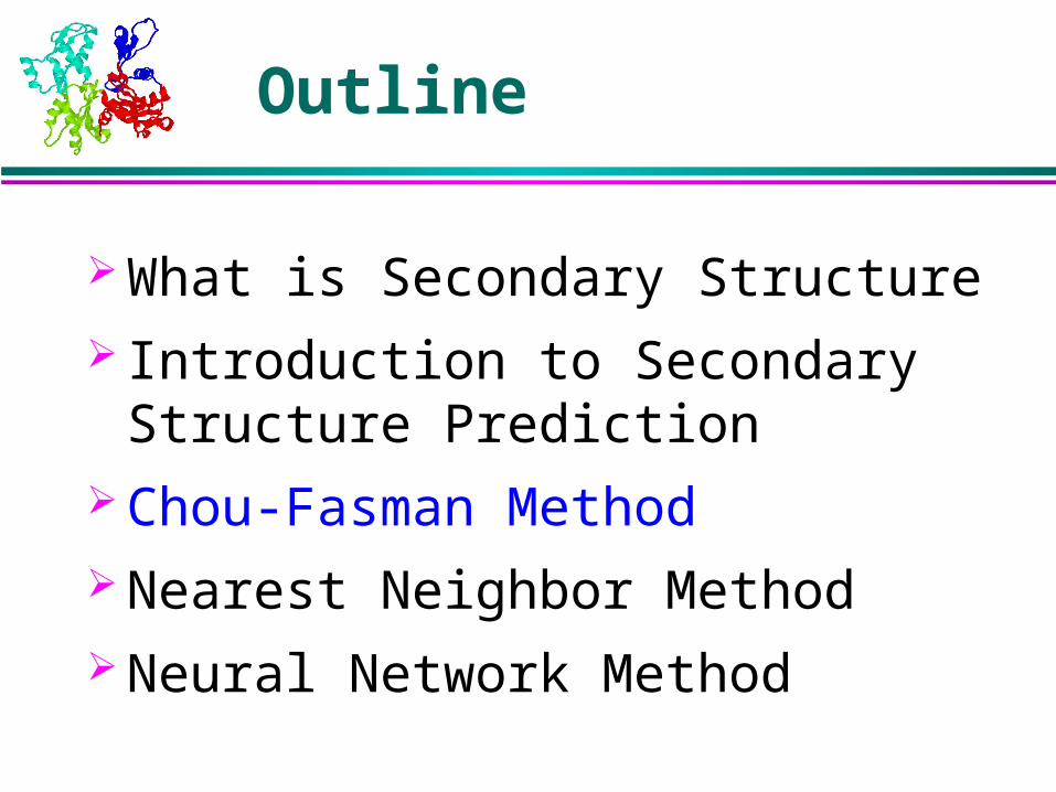
Outline

What is Secondary Structure Introduction to Secondary Structure

Prediction Chou-Fasman Method Nearest Neighbor Method Neural Network Method

Structures in Protein

Language:

Letters Words Sentences

Protein:

Residues Secondary Structure Tertiary Structure

helix

Single protein chain (local) Shape maintained by

intramolecular H bondingbetween -C=O and H-N-

sheet

Several protein chains

Shape maintained byintramolecular H bondingbetween chains

Non-local on protein sequence

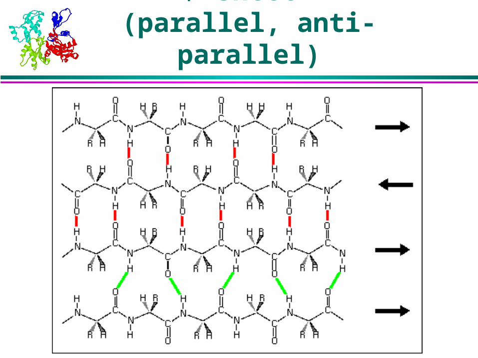
-sheet (parallel, anti-parallel)

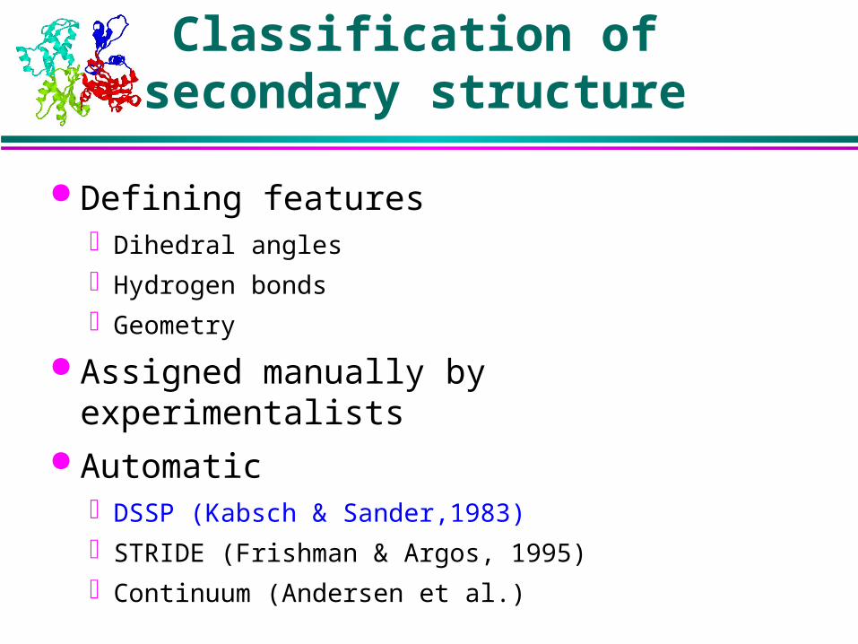
Classification ofsecondary structure

Defining featuresDihedral angles

Hydrogen bonds

Geometry

Assigned manually by experimentalists Automatic

DSSP (Kabsch & Sander,1983)

STRIDE (Frishman & Argos, 1995)

Continuum (Andersen et al.)

Classification

Eight states from DSSP H: helix

G: 310 helix

I: -helix

E: strand

B: bridge

T: turn

S: bend

C: coil

CASP Standard H = (H, G, I), E = (E, B), C = (C, T, S)

24 26 E H < S+ 0 0 132 25 27 R H < S+ 0 0 125 26 28 N < 0 0 41 27 29 K 0 0 197 28 ! 0 0 0 29 34 C 0 0 73 30 35 I E -cd 58 89B 9 31 36 L E -cd 59 90B 2 32 37 V E -cd 60 91B 0 33 38 G E -cd 61 92B 0

Dihedral angles

Ramachandran plot (alpha)

Ramachandran plot (beta)

Outline

What is Secondary Structure Introduction to Secondary Structure

Prediction Chou-Fasman Method Nearest Neighbor Method Neural Network Method

What is secondary structure prediction?

Given a protein sequence (primary structure)

GHWIATHWIATRGQLIREAYEDYGQLIREAYEDYRHFSSSSECPFIP

Predict its secondary structure content

(C=Coils H=Alpha Helix E=Beta Strands)

CEEEEEEEEEECHHHHHHHHHHHHHHHHHHHHHHCCCHHHHCCCCCC

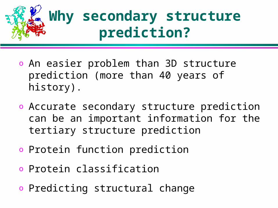
Why secondary structure prediction?

o An easier problem than 3D structure prediction (more than 40 years of history).

o Accurate secondary structure prediction can be an important information for the tertiary structure prediction

o Protein function prediction

o Protein classification

o Predicting structural change

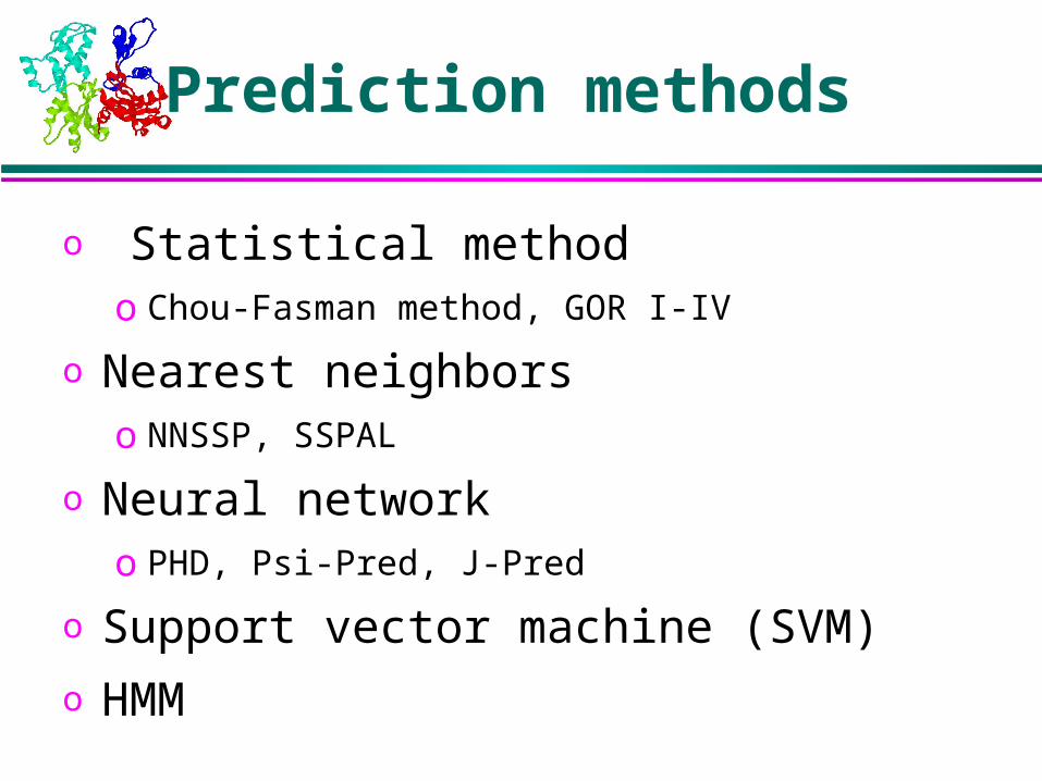
Prediction methods

o Statistical methodo Chou-Fasman method, GOR I-IV

o Nearest neighborso NNSSP, SSPAL

o Neural networko PHD, Psi-Pred, J-Pred

o Support vector machine (SVM)

o HMM

Accuracy measure

Three-state prediction accuracy: Q3

correctly predicted residues number of residues

3Q

A prediction of all loop: Q3 ~ 40%

Correlation coefficients

Improvement of accuracy

1974 Chou & Fasman ~50-53%

1978 Garnier 63%

1987 Zvelebil 66%

1988 Qian & Sejnowski 64.3%

1993 Rost & Sander 70.8-72.0%

1997 Frishman & Argos <75%

1999 Cuff & Barton 72.9%

1999 Jones 76.5%

2000 Petersen et al. 77.9%

0

5

10

15

20

25

30 40 50 60 70 80 90 100

PSIPREDSSproPROFPHDpsiJPred2PHD

Per

centa

ge

of

all

150

pro

tein

s

Percentage correctly predicted residues per protein

Prediction accuracy (EVA)

How far can we go?

Currently ~76% 1/5 of proteins with more than 100 homologs

>80% Assignment is ambiguous (5-15%).

non-unique protein structures, H-bond cutoff, etc.

Some segments can have multiple structure types.

Different secondary structures between homologues (~12%). Prediction limit 88%.

Non-locality.

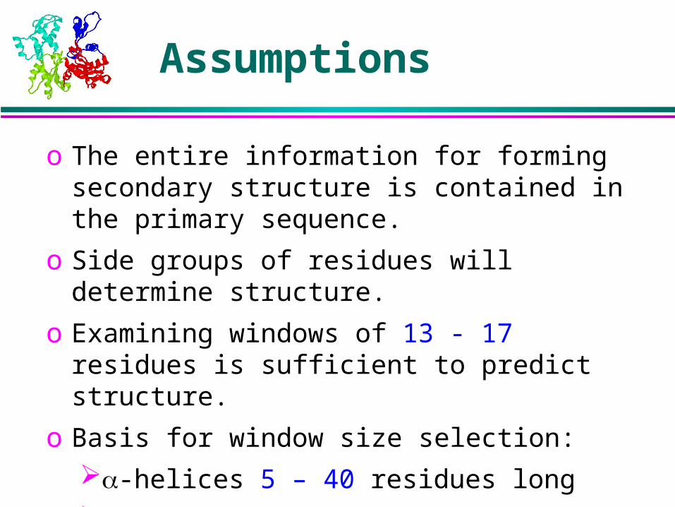
Assumptions

o The entire information for forming secondary structure is contained in the primary sequence.

o Side groups of residues will determine structure.

o Examining windows of 13 - 17 residues is sufficient to predict structure.

o Basis for window size selection:

-helices 5 – 40 residues long

-strands 5 – 10 residues long

Outline

What is Secondary Structure Introduction to Secondary Structure

Prediction Chou-Fasman Method Nearest Neighbor Method Neural Network Method

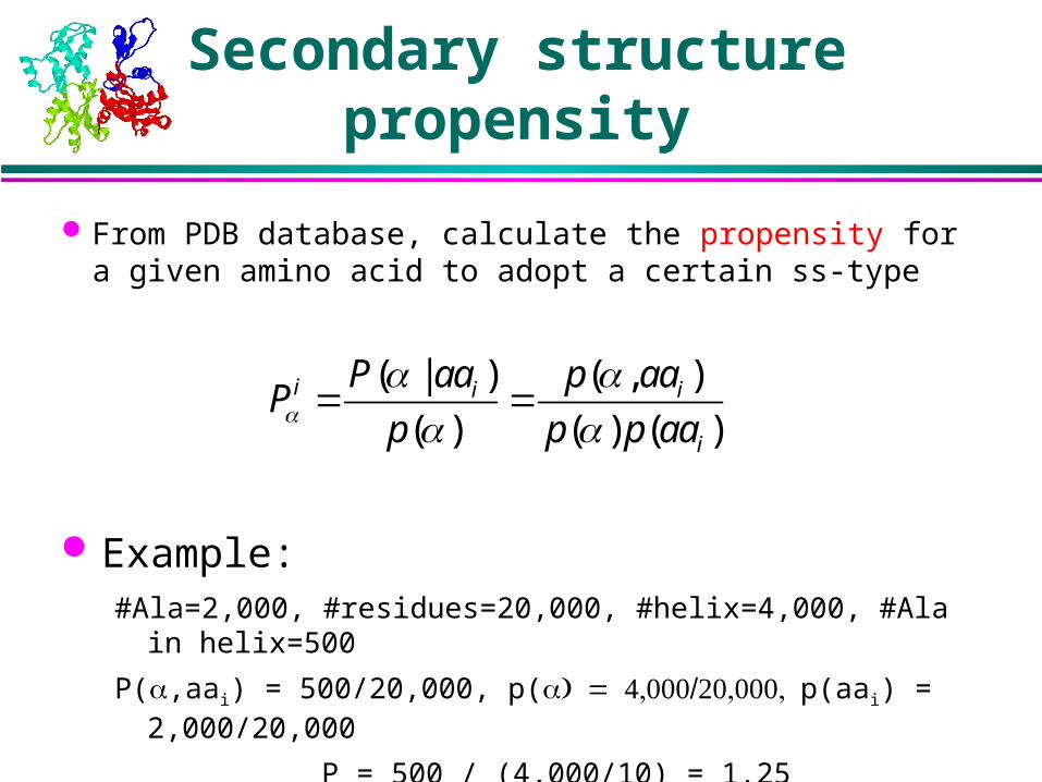
Secondary structure propensity

From PDB database, calculate the propensity for a given amino acid to adopt a certain ss-type

( | ) ( , )

( ) ( ) ( )i i i

i

P aa p aaP

p p p aa

Example:#Ala=2,000, #residues=20,000, #helix=4,000, #Ala in helix=500

P(,aai) = 500/20,000, p(p(aai) = 2,000/20,000

P = 500 / (4,000/10) = 1.25

Chou-Fasman algorithm

Helix, Strand1. Scan for window of 6 residues where average score > 1 (4

residues for helix and 3 residues for strand)

2. Propagate in both directions until 4 (or 3) residue window with mean propensity < 1

3. Move forward and repeat

Conflict solutionAny region containing overlapping alpha-helical and beta-strand assignments are taken to be helical if the average P(helix) > P(strand). It is a beta strand if the average P(strand) > P(helix).

Accuracy: ~50% ~60%

GHWIATRGQLIREAYEDYRHFSSECPFIP

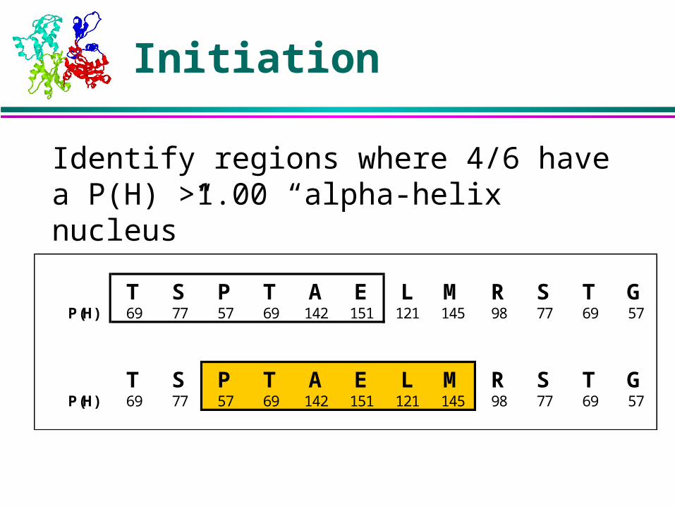
Initiation

T S P T A E L M R S T GP(H) 69 77 57 69 142 151 121 145 98 77 69 57

T S P T A E L M R S T GP(H) 69 77 57 69 142 151 121 145 98 77 69 57

Identify regions where 4/6 have a P(H) >1.00 “alpha-helix nucleus”

Propagation

T S P T A E L M R S T GP(H) 69 77 57 69 142 151 121 145 98 77 69 57

Extend helix in both directions until a set of four residues have an average P(H) <1.00.

Outline

What is Secondary Structure Introduction to Secondary Structure

Prediction Chou-Fasman Method Nearest Neighbor Method Neural Network Method

Nearest neighbor method

o Predict secondary structure of the central residue of a given segment from homologous segments (neighbors)(i) From database, find some number of the closest

sequences to a subsequence defined by a window around the central residue, or

(ii) Compute K best non-intersecting local alignments of a query sequence with each sequence.

o Use max (n, n, nc) for neighbor consensus or max(s, s, sc) for consensus sequence hits

Environment preference score

Each amino acid has a preference to a specific structural environments.

Structural variables: secondary structure, solvent accessibility

Non-redundant protein structure database: FSSP

( | ) ( , )( , ) log log

( ) ( ) ( )i j i j

i i j

p aa E p aa ES i j

p aa p aa p E

“Singleton” score matrix

Helix Sheet Loop Buried Inter Exposed Buried Inter Exposed Buried Inter ExposedALA -0.578 -0.119 -0.160 0.010 0.583 0.921 0.023 0.218 0.368ARG 0.997 -0.507 -0.488 1.267 -0.345 -0.580 0.930 -0.005 -0.032ASN 0.819 0.090 -0.007 0.844 0.221 0.046 0.030 -0.322 -0.487ASP 1.050 0.172 -0.426 1.145 0.322 0.061 0.308 -0.224 -0.541CYS -0.360 0.333 1.831 -0.671 0.003 1.216 -0.690 -0.225 1.216GLN 1.047 -0.294 -0.939 1.452 0.139 -0.555 1.326 0.486 -0.244GLU 0.670 -0.313 -0.721 0.999 0.031 -0.494 0.845 0.248 -0.144GLY 0.414 0.932 0.969 0.177 0.565 0.989 -0.562 -0.299 -0.601HIS 0.479 -0.223 0.136 0.306 -0.343 -0.014 0.019 -0.285 0.051ILE -0.551 0.087 1.248 -0.875 -0.182 0.500 -0.166 0.384 1.336LEU -0.744 -0.218 0.940 -0.411 0.179 0.900 -0.205 0.169 1.217LYS 1.863 -0.045 -0.865 2.109 -0.017 -0.901 1.925 0.474 -0.498MET -0.641 -0.183 0.779 -0.269 0.197 0.658 -0.228 0.113 0.714PHE -0.491 0.057 1.364 -0.649 -0.200 0.776 -0.375 -0.001 1.251PRO 1.090 0.705 0.236 1.249 0.695 0.145 -0.412 -0.491 -0.641SER 0.350 0.260 -0.020 0.303 0.058 -0.075 -0.173 -0.210 -0.228THR 0.291 0.215 0.304 0.156 -0.382 -0.584 -0.012 -0.103 -0.125TRP -0.379 -0.363 1.178 -0.270 -0.477 0.682 -0.220 -0.099 1.267TYR -0.111 -0.292 0.942 -0.267 -0.691 0.292 -0.015 -0.176 0.946VAL -0.374 0.236 1.144 -0.912 -0.334 0.089 -0.030 0.309 0.998

Total score

Alignment score is the sum of score in a window of length l:

/ 2

/ 2

( , ) [ ( , ) ( , )]l

k l

Score i j M i k j k cS i k j k

T R G Q L I R

i-4 i-3 i-2 i-1 i i+1 i+2 i+3 i+4

E A Y E D Y R H F S S E C P F I P

. . .E C Y E Y B R H R . . . . j-4 j-3 j-2 j-1 j j+1 j+2 j+3 j+4

| | | | |

L H H H H H H L L

Neighbors

1 - L H H H H H H L L - S1

2 - L L H H H H H L L - S2

3 - L E E E E E E L L - S3

4 - L E E E E E E L L - S4

n - L L L L E E E E E - Sn

n+1 - H H H L L L E E E - Sn+1

:

max (n, n, nL) or max (s, s, sL)

Evolutionary information

“All naturally evolved proteins with more than 35% pairwise identical residues over more than 100 aligned residues have similar structures.”

Stability of structure w.r.t. sequence divergence (<12% difference in secondary structure).

Position-specific sequence profile, containing crucial information on evolution of protein family, can help secondary structure prediction (increase information content).

Gaps rarely occur in helix and strand. ~1.4%/year increase in Q3 due to database growth

during past ~10 years.

How to use it

Sequence-profile alignment. Compare a sequence against protein family. More specific. BLAST vs. PSI-BLAST. Look up PSSM instead of PAM or BLOSUM.

/ 2

/ 2

( , ) [ ( , ) ( , )]l

k l

Score i j PSSM j k i k cS i k j k

position

amino acid type

Outline

What is Secondary Structure Introduction to Secondary Structure

Prediction Chou-Fasman Method Nearest Neighbor Method Neural Network Method

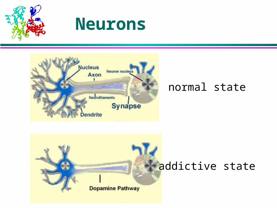
Neurons

normal state

addictive state

Neural network

Input signals are summed

and turned into zero or one

3.

J1

J2

J3

J4

Feed-forward multilayer network

Input layer Hidden layer Output layer

neurons

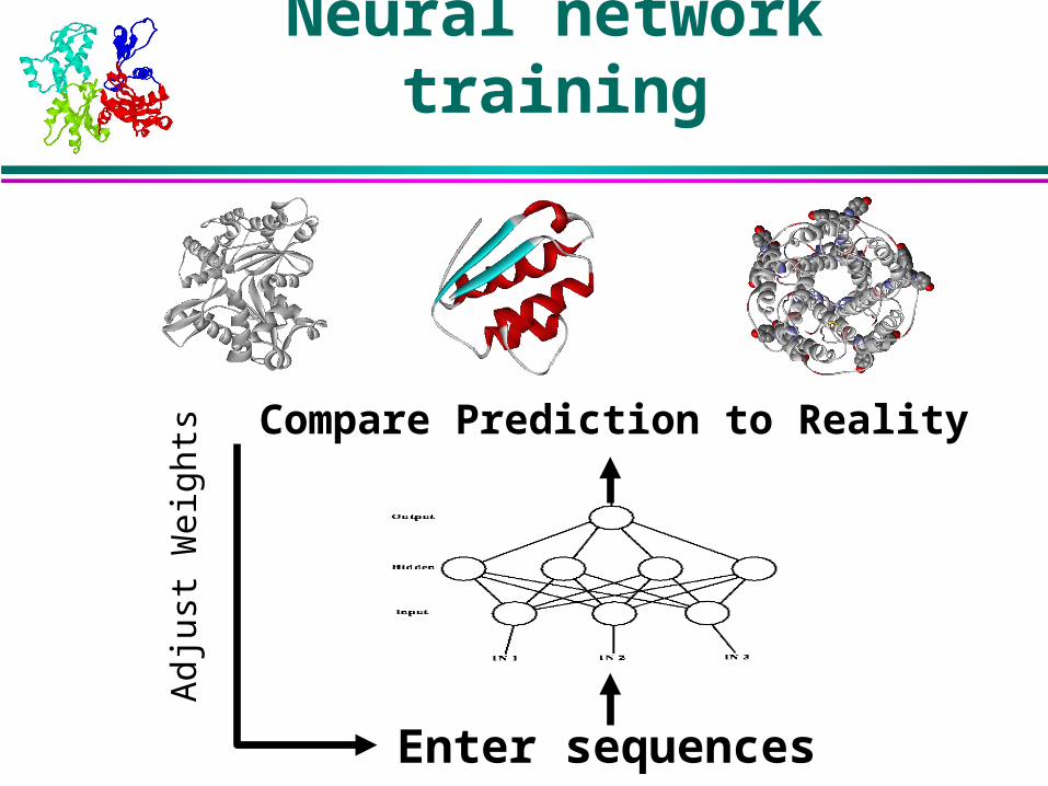
Enter sequences

Compare Prediction to Reality

Adj

ust W

eigh

ts

Neural network training

J 11

J 12

1

1

1

0

out0 = in1J 11 in2J 12 +

out = tanh (out0)

Simple Neural Network

Simple neural network

Error = | out_net – out_desired |

1

0

0

1

1

1

1

1

.

1

- 1

21- 1- 2

o u t

in

1

0

0

1

0

1

1

2

1

0

0

1

- 1

1

1

2+?

Training a neural network

Error

J unctions

Simple Neural NetworkWith Hidden Layer

out i fij

2 J fjk

1 Jk

kin

j

Simple neural network with hidden

layer

ACDEFGHIKLMNPQRSTVWY.

H

E

L

D (L)

R (E)

Q (E)

G (E)

F (E)

V (E)

P (E)

A (H)

A (H)

Y (H)

V (E)

K (E)

K (E)

Neural network for secondary structure

PsiPred

D. Jones, J. Mol. Boil. 292, 195 (1999). Method : Neural network Input data : PSSM generated by PSI-BLAST Bigger and better sequence database

Combining several database and data filtering

Training and test sets preparation Secondary structure prediction only makes sense for proteins

with no homologous structure.

No sequence & structural homologues between training and test sets by PSI-BLAST (mimicking realistic situation).

Psi-Pred (details)

Window size = 15 Two networks First network (sequence-to-structure):

315 = (20 + 1) 15 inputs extra unit to indicate where the windows spans either N or C terminus Data are scaled to [0-1] range by using 1/[1+exp(-x)] 75 hidden units 3 outputs (H, E, L)

Second network (structure-to-structure): Structural correlation between adjacent sequences 60 = (3 + 1) 15 inputs 60 hidden units 3 outputs

Accuracy ~76%

Reading Assignments

Suggested reading: Chapter 15 in “Current Topics in

Computational Molecular Biology, edited by Tao Jiang, Ying Xu, and Michael Zhang. MIT Press. 2002.”

Optional reading: Review by Burkhard Rost:

http://cubic.bioc.columbia.edu/papers/2003_rev_dekker/paper.html

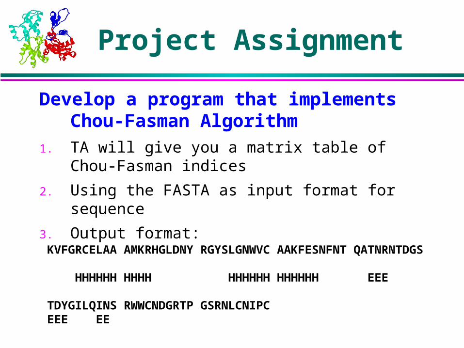
Develop a program that implements Chou-Fasman Algorithm

1. TA will give you a matrix table of Chou-Fasman indices

2. Using the FASTA as input format for sequence

3. Output format:

Project Assignment

KVFGRCELAA AMKRHGLDNY RGYSLGNWVC AAKFESNFNT QATNRNTDGS HHHHHH HHHH HHHHHH HHHHHH EEE

TDYGILQINS RWWCNDGRTP GSRNLCNIPC EEE EE