Embed Size (px)
Citation preview
Protocol Design, Testing and
Diagnosis towards Dependable
Wireless Sensor Networks
XIONG, Junjie
A Thesis Submitted in Partial Fulfilment
of the Requirements for the Degree of
Doctor of Philosophy
in
Computer Science and Engineering
The Chinese University of Hong Kong
September 2012

Thesis/Assessment Committee
Professor John Chi Shing LUI (Chair)
Professor Michael Rung Tsong LYU (Thesis Supervisor)
Professor Fung Yu YOUNG (Thesis Supervisor)
Professor Ho Man LEE (Committee Member)
Professor Bin XIAO (External Examiner)
Abstract of thesis entitled:
Protocol Design, Testing and Diagnosis towards Dependable Wireless Sensor
Networks
Submitted by XIONG, Junjie
for the degree of Doctor of Philosophy
at The Chinese University of Hong Kong in September 2012
This thesis investigates the protocol design, testing, and diagnosis of Wireless
Sensor Networks (WSNs) to achieve dependable WSNs.
In the aspect of protocol design, we focus on the MAC (Medium Access
Control) layer protocol design. First, we propose an efficient MAC protocol
RAS (routing and application based scheduling protocol) for underwater acoustic
sensor networks (UWASNs), a type of WSNs that are deployed in the water.
Utilizing the medium propagation difference between UWASNs and terrestrial
wireless sensor networks (TWSNs), RAS performs parallel transmissions which
would definitely result in collisions in TWSNs. It schedules the transmissions
with different priorities by allocating longer time to heavier-traffic sensor nodes.
The priority mechanism also benefits the fairness performance. Second, we tackle
the unreliability problem caused by the packet loss in UWASNs. Based on the
previously designed RAS, we propose a reliable RAS called RRAS that obtains
a tradeoff between the reliability and the efficiency. RRAS applies an ACK and
retransmission mechanism that is different from the traditional one, so that it can
maintain a comparable throughput while improving reliability.
Third, in the area of protocol testing, we design RealProct (reliable Protocol
conformance testing with Real sensor nodes), a novel and reliable framework
for performing protocol conformance testing in WSNs, i.e., testing the protocol
implementations against their specifications. With real sensor nodes, RealProct
can ensure that the testing scenarios are as close to the real deployment as possible.
To save the hardware cost and control efforts required by testing with large-scale
real deployments, RealProct virtualizes a network with any topology and generates
non-deterministic events using only a small number of sensor nodes. In addition,
test execution and verdict are optimized to minimize the number of test case runs,
while guaranteeing satisfactory false positive and false negative rates.
Finally, we propose MDiag, a Mobility-assisted Diagnosis approach that
employs smartphones to patrol the WSNs and diagnose failures. Diagnosing with
a smartphone which is not a component of WSNs does not intrude the execution
of the WSNs as most of the existing diagnosis methods. Moreover, patrolling the
smartphone in the WSNs to investigate failures is more efficient than deploying
another diagnosis network. During the patrol, packets exchanged in the WSNs are
collected and then analyzed by our implemented packet decoder. Statistical rules
are also designed to guide the detection of abnormal cases. Aiming at improving
the patrol efficiency, a patrol approach MSEP (maximum snooping efficiency
patrol) is proposed. We compare MSEP with a naive method, the greedy method,
and a baseline method, and demonstrate that MSEP is better in increasing the
detection rate and reducing the patrol time than other methods.
We perform extensive evaluations to verify the proposed techniques and
algorithms, and the results confirm their advantages in achieving dependable
WSNs.
ii

¥'阻B冊人@ H :
面向可靠的無線傳感器網絡的協議設計,測試和診斷
提交人:熊捃潔
修讀學位:哲學博士
香港中文大學,二零一二年六月
摘要:本文研究面向可靠的無線傳感器網絡的協議設計,測試和診斷。
在協議設計方面,我們集中研究媒體接入層的協議設計。首先,我們爲水下
無線傳感器網絡提出一個有效的媒體接入層協議RAS�這個協議利用了水下
無線傳感器網絡和地面無線傳感器網絡的媒體傳輸時延的差別,采用了並行
傳輸的優先級方法。由于會導致碰撞,這種並行傳輸的方法不能被用在地面
無線傳感器網絡中。該方法爲高負荷的傳感器節點分配更長的傳輸時間。這
種具有優先級的機制也同時提高了公平方面的性能。第二,我們處理水下無
線傳感器網絡中由于報文丟失導致的不可靠的問題。基于之前提出的協議
RAS,我們提出了可靠的RAS協議。該協議可以在可靠性和有效性方便達到
一個平衡。它裏面的報文確認和重傳機制同傳統的方法不同,所以它可以在
提高可靠性的同時保證吞吐量不會被大幅降低。
第三,在協議測試方面,我們設計了 RealProct,一種新的可靠的用于無線傳
感器網絡的一致性協議測試(測試協議實現是否符合協議規範)的架構。
RealProct采用了實際的傳感器節點來保證測試盡可能的接近實際部署。爲了
節省使用大規模實際部署來測試的硬件成本和控制成本,RealProct使用少量
傳感器節點虛擬各樣的拓撲結構和事件。同時,測試執行和裁決算法也用于
最小化測試用例執行次數,並保證假陰和假陽錯誤低于給定值。
最後,我們提出了 MDmg,一種使用移動智能手機巡視無線傳感器網絡並診
斷網絡錯誤的方法。由于該智能手機不是無線傳感器網絡的組成部分,因此
該診斷不會像其它已有的診斷方法那樣影響原無線傳感器網絡的運行。並且,
使用智能手機巡視並診斷無線傳感器網絡比部署另一個用于診斷的網絡更有
效。在巡視過程中,無線傳感器網絡所交互的報文被收集起來,然後被我們
所設計的報文解析器所分析。然後,我們設計了統計性規則來指導異常現象
的診斷。爲了提高巡視效率,我們提出了一個巡視方法MSEP�
我們做了大量實驗驗證以上提出的方法和算法,結果表明它們在達到可靠性
無線傳感器網絡的目標上很有效。
iii
Acknowledgement
I would like to express my greatest thanks to my supervisors, Prof. Michael R.
Lyu, Prof. Kam-Wing Ng, and Prof Evangeline F.Y YOUNG, for their advice,
patience, understanding, and encouragement. Without their support, this thesis
would not have been possible. They taught me how to do the research, and how
to maintain a positive attitude toward research. They have not only promoted my
techniques, but also shaped my mind. They are always my mentors guiding me on
my road towards an academic career and the unexplored world.
I would also like to thank my thesis committee members, Prof. John Lui,
Prof. Jimmy Lee, and Prof. Bin Xiao for their precious time to serve as my thesis
assessment committee members during my PHD study. Their comments are and
suggestions on my work are detailed and very constructive. They helped me a lot
in improving my research.
I am happy that I had the chances to work with Dr Edith C.-H. Ngai at Uppsala
University. I warmly thank her for supporting me in doing research on the protocol
testing and diagnosis in wireless sensor networks. Her advice is important and
helpful in improving my research work. Working with her is always a pleasure
I would like to thank my colleagues and friends. Especially, I want to thank
Yangfan Zhou for his great help and guidance to my work in my whole PHD study.
Thank Xinyu Chen for his patient suggestions and valuable corrections. Thank
Wujie Zheng, Xin Xin, Zibin Zheng, Haiqin Yang, Hao Ma, Yilei Zhang, Kang
Yu, and many others for their encouragement and kind help.
iv

I am grateful to my mother and my husband for their unlimited love and strong
support.
v

To my family.
vi
Contents
Abstract i
Acknowledgement iv
1 Introduction and Background Study 1
1.1 Wireless Sensor Networks (WSNs) . . . . . . . . . . . . . . . . . 1
1.1.1 Sensor Node . . . . . . . . . . . . . . . . . . . . . . . . 5
1.1.2 The Base Station (BS) . . . . . . . . . . . . . . . . . . . 8
1.1.3 The Operating System (OS) of the Sensor Node . . . . . . 8
1.1.4 The Protocol Design of WSNs . . . . . . . . . . . . . . . 11
1.2 Thesis Scope and Contributions . . . . . . . . . . . . . . . . . . 20
1.2.1 Protocol Design . . . . . . . . . . . . . . . . . . . . . . . 20
1.2.2 Protocol Testing . . . . . . . . . . . . . . . . . . . . . . 22
1.2.3 Protocol Diagnosis . . . . . . . . . . . . . . . . . . . . . 23
1.3 Thesis Organization . . . . . . . . . . . . . . . . . . . . . . . . . 23
2 An Efficient MAC Protocol Design 25
2.1 Introduction . . . . . . . . . . . . . . . . . . . . . . . . . . . . . 26
2.2 Related Work . . . . . . . . . . . . . . . . . . . . . . . . . . . . 28
2.3 RAS Overview . . . . . . . . . . . . . . . . . . . . . . . . . . . 29
2.3.1 Scheduling Element . . . . . . . . . . . . . . . . . . . . 32
2.4 The Scheduling Problem in UWASNs . . . . . . . . . . . . . . . 34
vii

2.4.1 Scheduling Principles . . . . . . . . . . . . . . . . . . . 34
2.4.2 Scheduling Problem Formulation . . . . . . . . . . . . . 35
2.4.3 Scheduling Problem Analysis . . . . . . . . . . . . . . . 37
2.5 RAS Protocol . . . . . . . . . . . . . . . . . . . . . . . . . . . . 38
2.5.1 Scheduling Algorithm of the RAS Protocol . . . . . . . . 38
2.5.2 Analysis of the RAS Protocol . . . . . . . . . . . . . . . 39
2.6 Performance Evaluation . . . . . . . . . . . . . . . . . . . . . . . 42
2.6.1 Schedule Length . . . . . . . . . . . . . . . . . . . . . . 42
2.6.2 Network Throughput . . . . . . . . . . . . . . . . . . . . 44
2.6.3 Average End-to-end Delay . . . . . . . . . . . . . . . . . 46
2.6.4 Average Maximum Queue Length per Node . . . . . . . . 47
2.7 Discussions and Conclusions . . . . . . . . . . . . . . . . . . . . 49
3 A Reliable MAC Protocol Design 51
3.1 Introduction . . . . . . . . . . . . . . . . . . . . . . . . . . . . . 52
3.2 Related Work . . . . . . . . . . . . . . . . . . . . . . . . . . . . 54
3.3 RRAS Protocol . . . . . . . . . . . . . . . . . . . . . . . . . . . 55
3.3.1 Overview of NACK-retransmission Mechanism . . . . . . 56
3.3.2 Retransmission Mechanism . . . . . . . . . . . . . . . . 57
3.3.3 Retransmission Time . . . . . . . . . . . . . . . . . . . . 59
3.4 Performance Evaluation . . . . . . . . . . . . . . . . . . . . . . . 61
3.4.1 Retransmission Time of RRAS . . . . . . . . . . . . . . . 62
3.4.2 Working Time of RRAS and RAS . . . . . . . . . . . . . 63
3.4.3 Success Rate of RRAS and RAS . . . . . . . . . . . . . . 64
3.4.4 Throughput of RRAS and RAS . . . . . . . . . . . . . . 65
3.5 Conclusions . . . . . . . . . . . . . . . . . . . . . . . . . . . . . 66
4 Reliable Protocol Conformance Testing 67
4.1 Introduction . . . . . . . . . . . . . . . . . . . . . . . . . . . . . 68
viii
4.2 Related Work . . . . . . . . . . . . . . . . . . . . . . . . . . . . 71
4.3 Protocol Conformance Testing . . . . . . . . . . . . . . . . . . . 73
4.3.1 PCT Process . . . . . . . . . . . . . . . . . . . . . . . . 74
4.3.2 PCT Architecture . . . . . . . . . . . . . . . . . . . . . . 75
4.4 Design of the RealProct Framework . . . . . . . . . . . . . . . . 76
4.5 RealProct Techniques . . . . . . . . . . . . . . . . . . . . . . . . 79
4.5.1 Topology Virtualization . . . . . . . . . . . . . . . . . . 80
4.5.2 Event Virtualization . . . . . . . . . . . . . . . . . . . . 81
4.5.3 Dynamic Test Execution . . . . . . . . . . . . . . . . . . 85
4.6 Generality of RealProct . . . . . . . . . . . . . . . . . . . . . . . 88
4.7 Evaluation . . . . . . . . . . . . . . . . . . . . . . . . . . . . . . 89
4.7.1 Detecting New Bugs in TCP . . . . . . . . . . . . . . . . 90
4.7.2 Detecting Previous Bugs in TCP . . . . . . . . . . . . . . 94
4.7.3 Testing Routing Protocol RMRP . . . . . . . . . . . . . . 98
4.8 Conclusions . . . . . . . . . . . . . . . . . . . . . . . . . . . . . 99
5 Mobility-assisted Diagnosis for WSNs 101
5.1 Introduction . . . . . . . . . . . . . . . . . . . . . . . . . . . . . 102
5.2 Related Work . . . . . . . . . . . . . . . . . . . . . . . . . . . . 105
5.3 MDiag Background . . . . . . . . . . . . . . . . . . . . . . . . . 108
5.3.1 Network Architecture . . . . . . . . . . . . . . . . . . . . 108
5.3.2 Failure Classification . . . . . . . . . . . . . . . . . . . . 108
5.4 MDiag Framework . . . . . . . . . . . . . . . . . . . . . . . . . 109
5.4.1 Packet Decoder Input and Output . . . . . . . . . . . . . 111
5.4.2 Statistical Rules on Packet Analysis . . . . . . . . . . . . 112
5.5 Coverage-oriented Smartphone Patrol Algorithms . . . . . . . . . 115
5.5.1 Naive Method (NM) . . . . . . . . . . . . . . . . . . . . 115
5.5.2 Greedy Method (GM) . . . . . . . . . . . . . . . . . . . 116
5.5.3 Maximum Snooping Efficiency Patrol (MSEP) . . . . . . 118
ix

5.6 Evaluations . . . . . . . . . . . . . . . . . . . . . . . . . . . . . 119
5.6.1 Permanent Failure Detection . . . . . . . . . . . . . . . . 121
5.6.2 Short-term Failure Detection . . . . . . . . . . . . . . . . 122
5.7 Conclusions . . . . . . . . . . . . . . . . . . . . . . . . . . . . . 130
6 Conclusions 132
Bibliography 136
x
List of Figures
1 The development, deployment, and maintenance of the WSN
applications. . . . . . . . . . . . . . . . . . . . . . . . . . . . . . iii
1.1 The typical architecture of a WSN. . . . . . . . . . . . . . . . . 2
1.2 The reference architecture of a sensor node. . . . . . . . . . . . . 5
1.3 The development of sensor nodes. . . . . . . . . . . . . . . . . . 6
1.4 The typical hardware architecture of a sensor node. ADC
represents analog-to-digital converter. . . . . . . . . . . . . . . . 7
1.5 A BS developed by Crossbow. . . . . . . . . . . . . . . . . . . . 9
1.6 The development, deployment, and maintenance of the WSN
applications. . . . . . . . . . . . . . . . . . . . . . . . . . . . . . 21
2.1 A data transaction process. . . . . . . . . . . . . . . . . . . . . . 26
2.2 Application topology for UWASNs. . . . . . . . . . . . . . . . . 30
2.3 RAS cycle. . . . . . . . . . . . . . . . . . . . . . . . . . . . . . 31
2.4 Data transmissions among 3 nodes in UWASNs. . . . . . . . . . . 33
2.5 RAS schedule length vs. lower bound schedule length. . . . . . . 43
2.6 Schedule ratio. . . . . . . . . . . . . . . . . . . . . . . . . . . . 44
2.7 Schedule length VS guardtime. . . . . . . . . . . . . . . . . . . . 45
2.8 Throughput comparison . . . . . . . . . . . . . . . . . . . . . . . 46
2.9 End-to-end delay comparison . . . . . . . . . . . . . . . . . . . . 47
2.10 Queue length comparison. . . . . . . . . . . . . . . . . . . . . . 48
xi
3.1 RRAS cycle. . . . . . . . . . . . . . . . . . . . . . . . . . . . . 56
3.2 Retransmission time. . . . . . . . . . . . . . . . . . . . . . . . . 62
3.3 Working time. . . . . . . . . . . . . . . . . . . . . . . . . . . . . 63
3.4 DATA transmission success rate. . . . . . . . . . . . . . . . . . . 64
3.5 Throughput. . . . . . . . . . . . . . . . . . . . . . . . . . . . . . 65
4.1 PCT testing process. . . . . . . . . . . . . . . . . . . . . . . . . 75
4.2 RealProct framework. . . . . . . . . . . . . . . . . . . . . . . . . 77
4.3 Topology virtualization demonstration. . . . . . . . . . . . . . . . 81
4.4 A topology for event virtualization. . . . . . . . . . . . . . . . . . 83
4.5 Testing devices. . . . . . . . . . . . . . . . . . . . . . . . . . . . 90
4.6 TCP three-way handshake. . . . . . . . . . . . . . . . . . . . . . 91
4.7 Test results of test case 1. . . . . . . . . . . . . . . . . . . . . . . 93
4.8 SYN packet loss. . . . . . . . . . . . . . . . . . . . . . . . . . . 95
4.9 SYN packet duplication. . . . . . . . . . . . . . . . . . . . . . . 97
5.1 A MDiag patrol scenario. The smartphone first visits sensor node
1, then sensor node 2, 3, 4, and 5. . . . . . . . . . . . . . . . . . . 103
5.2 Failure classification. . . . . . . . . . . . . . . . . . . . . . . . . 109
5.3 MDiag framework. . . . . . . . . . . . . . . . . . . . . . . . . . 110
5.4 Raw packet structure. . . . . . . . . . . . . . . . . . . . . . . . . 111
5.5 Statistical results. . . . . . . . . . . . . . . . . . . . . . . . . . . 111
5.6 Network topology I. The smartphone stays near sensor node 2. . . 116
5.7 Patrol set selection of GM (sub-figure a) and MSEP (sub-figure b).
The blue circle is put into the patrol set. . . . . . . . . . . . . . . 117
5.8 Network topology II. The smartphone patrols the sensor nodes in
the network. . . . . . . . . . . . . . . . . . . . . . . . . . . . . . 123
5.9 Lasting time of the abnormal cases. . . . . . . . . . . . . . . . . 124
5.10 Detection probability of AC1. . . . . . . . . . . . . . . . . . . . 127
xii

5.11 Detection probability of AC3. . . . . . . . . . . . . . . . . . . . 128
5.12 Detection probability of AC2. . . . . . . . . . . . . . . . . . . . 129
5.13 Detection probability of AC4, AC5, AC6, and AC7 when the
working time is 200s. . . . . . . . . . . . . . . . . . . . . . . . . 130
5.14 Detection probability of all ACs. . . . . . . . . . . . . . . . . . . 131
xiii

List of Tables
1.1 Radio and storage parameters for a Mica sensor and an Iris sensor
node. . . . . . . . . . . . . . . . . . . . . . . . . . . . . . . . . . 8
2.1 Parameters for data transmissions. . . . . . . . . . . . . . . . . . 27
2.2 Tt and Tp for TWSNs and UWASNs. . . . . . . . . . . . . . . . . 27
2.3 Notations. . . . . . . . . . . . . . . . . . . . . . . . . . . . . . . 34
5.1 Our statistical rules are a subset of the specification-based rules. . 113
5.2 Statistical rules for a typical WSN application. . . . . . . . . . . . 114
5.3 Parameter comparison for all the algorithms. . . . . . . . . . . . . 126
xiv

Chapter 1
Introduction and Background Study
1.1 Wireless Sensor Networks (WSNs)
Recent advances in sensors, VLSI (Very-large-scale integration), MEMS
(Micro-electro-mechanical systems), as well as wireless communication
technologies have made it possible to build powerful wireless sensor networks
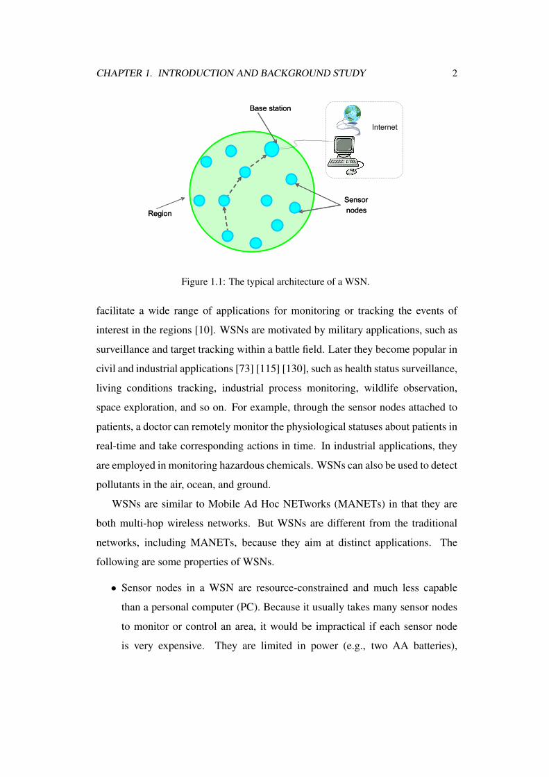
(WSNs) [10]. As shown in Figure 1.1, a WSN is composed of many low-cost
and small wireless sensor nodes (sensor nodes in short). These sensor nodes are
distributed in a designated region. Note that their positions need not be engineered
or pre-determined so that they can be randomly deployed in inaccessible terrains
and adverse areas. For example, the sensor nodes can be dropped into a forest
by the helicopter to monitor the temperature and issue fire breakout warnings.
This also means that the sensor nodes should be able to self-organize into a
wireless network. They collect information about the region and transmit it to
the base station (BS), a centralized and more capable station, through multi-hop
communications. Then the BS can send the information to any remote end in the
Internet. Unlike traditional networks, WSNs depend on dense deployment and
co-ordination to carry out their tasks.
As a result of various sensing abilities and wireless connection, WSNs greatly
1
CHAPTER 1. INTRODUCTION AND BACKGROUND STUDY 2
RegionRegion
Base station
Sensor
nodes
Base station
Sensor
nodes
Internet
Figure 1.1: The typical architecture of a WSN.
facilitate a wide range of applications for monitoring or tracking the events of
interest in the regions [10]. WSNs are motivated by military applications, such as
surveillance and target tracking within a battle field. Later they become popular in
civil and industrial applications [73] [115] [130], such as health status surveillance,
living conditions tracking, industrial process monitoring, wildlife observation,
space exploration, and so on. For example, through the sensor nodes attached to
patients, a doctor can remotely monitor the physiological statuses about patients in
real-time and take corresponding actions in time. In industrial applications, they
are employed in monitoring hazardous chemicals. WSNs can also be used to detect
pollutants in the air, ocean, and ground.
WSNs are similar to Mobile Ad Hoc NETworks (MANETs) in that they are
both multi-hop wireless networks. But WSNs are different from the traditional
networks, including MANETs, because they aim at distinct applications. The
following are some properties of WSNs.
• Sensor nodes in a WSN are resource-constrained and much less capable
than a personal computer (PC). Because it usually takes many sensor nodes
to monitor or control an area, it would be impractical if each sensor node
is very expensive. They are limited in power (e.g., two AA batteries),
CHAPTER 1. INTRODUCTION AND BACKGROUND STUDY 3
computational capacities, and memory. After their deployment, human
attendance is usually not involved. Hence power cannot be conveniently
recharged. Therefore, while traditional networks aim to achieve high quality
of service (QoS) provisions, sensor network research must focus primarily
on power conservation to maximize the network lifetime. Meanwhile, since
the bandwidth of WSNs (250 kbps for an Iris sensor node [1]) is not as high
as the wired network and WiFi (100 Mbps as a moderate value), how to avoid
collisions and improve throughput is another concern.
• Sensor nodes in a WSN are able to self-organize to communicate through a
wireless communications. In WSN applications, the sensor nodes are usually
randomly deployed at a place where human cannot get close or when the
sensor node number is so large that manual placing is laborious. A typical
way of deployment in a forest would be tossing the sensor nodes from an
airplane. In most cases, once deployed, WSNs allow no human intervention.
In such a situation, it is up to the sensor nodes to identify its connectivity
and distribution. They are responsible for self-organizing into a wireless
communication network. As a result, the medium access control (MAC)
protocol and routing protocol are very important for a sensor node to detect
its neighbors and set up a route to the destination. These protocols should
be robust enough to tolerate certain level of corner cases. For example, a
rebooted sensor node should be able to rejoin the WSN other than being
isolated. A malfunctioned sensor node should not damage the routing for a
long period. Otherwise, the WSN applications may suffer failures and break
down easily.
• Sensor nodes in a WSN are subjected to dynamic changes. Some
already-deployed WSNs may be expanded by adding a collection of sensor
nodes. Through communications, these newly joined sensor nodes affect
the execution of the original WSN. In addition, because of their adverse
CHAPTER 1. INTRODUCTION AND BACKGROUND STUDY 4
working environment and limited capabilities, sensor nodes are prone to
malfunction or die of energy depletion. If the sensor nodes get back to
normal, they will rejoin the network. These common joining in and quitting
actions cause dynamic changes in the networks. Furthermore, the volatile
environment may cause random packet loss during the wireless transmission,
which disturbs the routing and degrade the data communication performance.
As a result, it is vital to improve the system reliability by adapting the WSNs
to these dynamic changes.
• WSNs are application-specific. WSNs are not designed to provide
general-purpose applications as the Internet [90]. Some applications are
time-sensitive, such as fire breakout surveillance, while others only require
regular monitoring, such as wildlife observation. Some applications require
a large amount of data transmission in a short interval whereas some are
satisfied with a low data rate. Moreover, since the main task WSNs take
is collecting data and transmitting the data to the BS in time, the protocol
design and operating system should be tailored to support such requirement.
As a result, WSN applications usually do not employ the standard TCP/IP
protocols, which would consume a lot of the limited resource in a sensor
node. Their key concern is the protocol design below the routing layer,
including the routing layer itself.
Realization of WSNs for different applications requires both hardware and
software support. In the following subsections, we first describe the main hardware
requirements in respects of the sensor nodes and the base station. Then, we
discuss the software necessities in terms of the operating system and the protocols.
The reference architecture of a sensor node is shown in Figure 1.2, in which the
shadowed rectangle represents the hardware while the rest is the software. It is
similar to the traditional PC architecture, but each part of it is different. For
example, the hardware is cost-effective and thus simpler. We will explain them
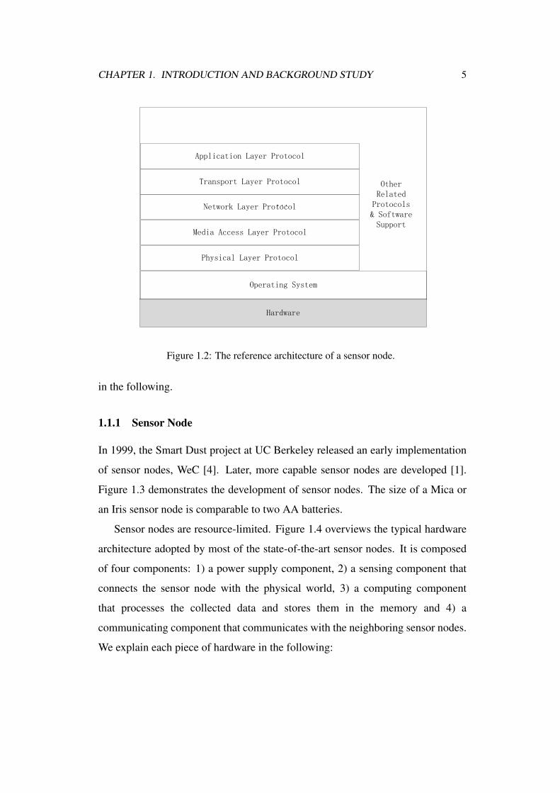
CHAPTER 1. INTRODUCTION AND BACKGROUND STUDY 5
Figure 1.2: The reference architecture of a sensor node.
in the following.
1.1.1 Sensor Node
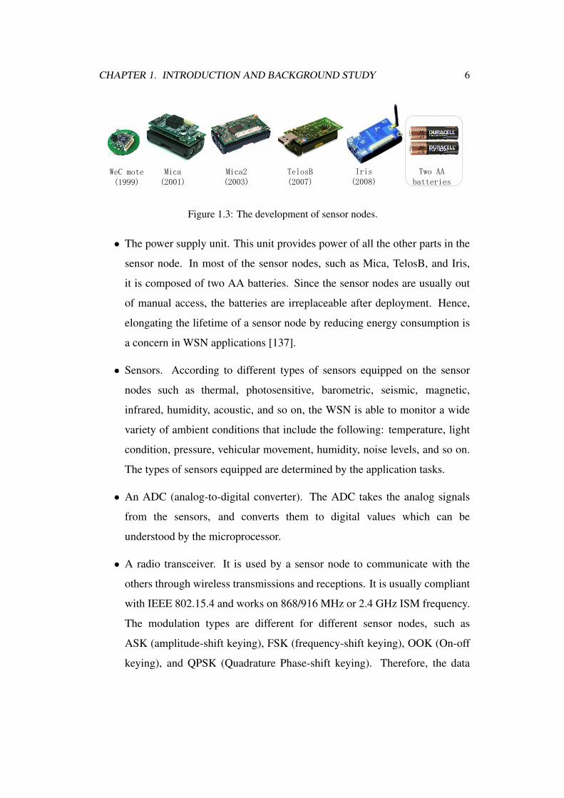
In 1999, the Smart Dust project at UC Berkeley released an early implementation
of sensor nodes, WeC [4]. Later, more capable sensor nodes are developed [1].
Figure 1.3 demonstrates the development of sensor nodes. The size of a Mica or
an Iris sensor node is comparable to two AA batteries.
Sensor nodes are resource-limited. Figure 1.4 overviews the typical hardware
architecture adopted by most of the state-of-the-art sensor nodes. It is composed
of four components: 1) a power supply component, 2) a sensing component that
connects the sensor node with the physical world, 3) a computing component
that processes the collected data and stores them in the memory and 4) a
communicating component that communicates with the neighboring sensor nodes.
We explain each piece of hardware in the following:
CHAPTER 1. INTRODUCTION AND BACKGROUND STUDY 6
Figure 1.3: The development of sensor nodes.
• The power supply unit. This unit provides power of all the other parts in the
sensor node. In most of the sensor nodes, such as Mica, TelosB, and Iris,
it is composed of two AA batteries. Since the sensor nodes are usually out
of manual access, the batteries are irreplaceable after deployment. Hence,
elongating the lifetime of a sensor node by reducing energy consumption is
a concern in WSN applications [137].
• Sensors. According to different types of sensors equipped on the sensor
nodes such as thermal, photosensitive, barometric, seismic, magnetic,
infrared, humidity, acoustic, and so on, the WSN is able to monitor a wide
variety of ambient conditions that include the following: temperature, light
condition, pressure, vehicular movement, humidity, noise levels, and so on.
The types of sensors equipped are determined by the application tasks.
• An ADC (analog-to-digital converter). The ADC takes the analog signals
from the sensors, and converts them to digital values which can be
understood by the microprocessor.
• A radio transceiver. It is used by a sensor node to communicate with the
others through wireless transmissions and receptions. It is usually compliant
with IEEE 802.15.4 and works on 868/916 MHz or 2.4 GHz ISM frequency.
The modulation types are different for different sensor nodes, such as
ASK (amplitude-shift keying), FSK (frequency-shift keying), OOK (On-off
keying), and QPSK (Quadrature Phase-shift keying). Therefore, the data
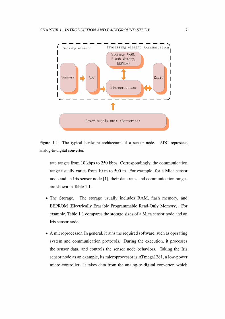
CHAPTER 1. INTRODUCTION AND BACKGROUND STUDY 7
Figure 1.4: The typical hardware architecture of a sensor node. ADC represents
analog-to-digital converter.
rate ranges from 10 kbps to 250 kbps. Correspondingly, the communication
range usually varies from 10 m to 500 m. For example, for a Mica sensor
node and an Iris sensor node [1], their data rates and communication ranges
are shown in Table 1.1.
• The Storage. The storage usually includes RAM, flash memory, and
EEPROM (Electrically Erasable Programmable Read-Only Memory). For
example, Table 1.1 compares the storage sizes of a Mica sensor node and an
Iris sensor node.
• A microprocessor. In general, it runs the required software, such as operating
system and communication protocols. During the execution, it processes
the sensor data, and controls the sensor node behaviors. Taking the Iris
sensor node as an example, its microprocessor is ATmega1281, a low-power
micro-controller. It takes data from the analog-to-digital converter, which

CHAPTER 1. INTRODUCTION AND BACKGROUND STUDY 8
Table 1.1: Radio and storage parameters for a Mica sensor and an Iris sensor node.
A Mica sensor node An Iris sensor node
Radio frequency 916 MHz kbps 2.4 GHz
Data rate 50 kbps 250 kbps
Communication range 60 m 300 m
RAM 4K bytes 8K bytes
Flash memory 128K bytes 128K bytes
EEPROM 4K bytes 4K bytes
can be stored to the storage or be sent to the radio transceiver. It can also get
data from the radio transceiver and the storage.
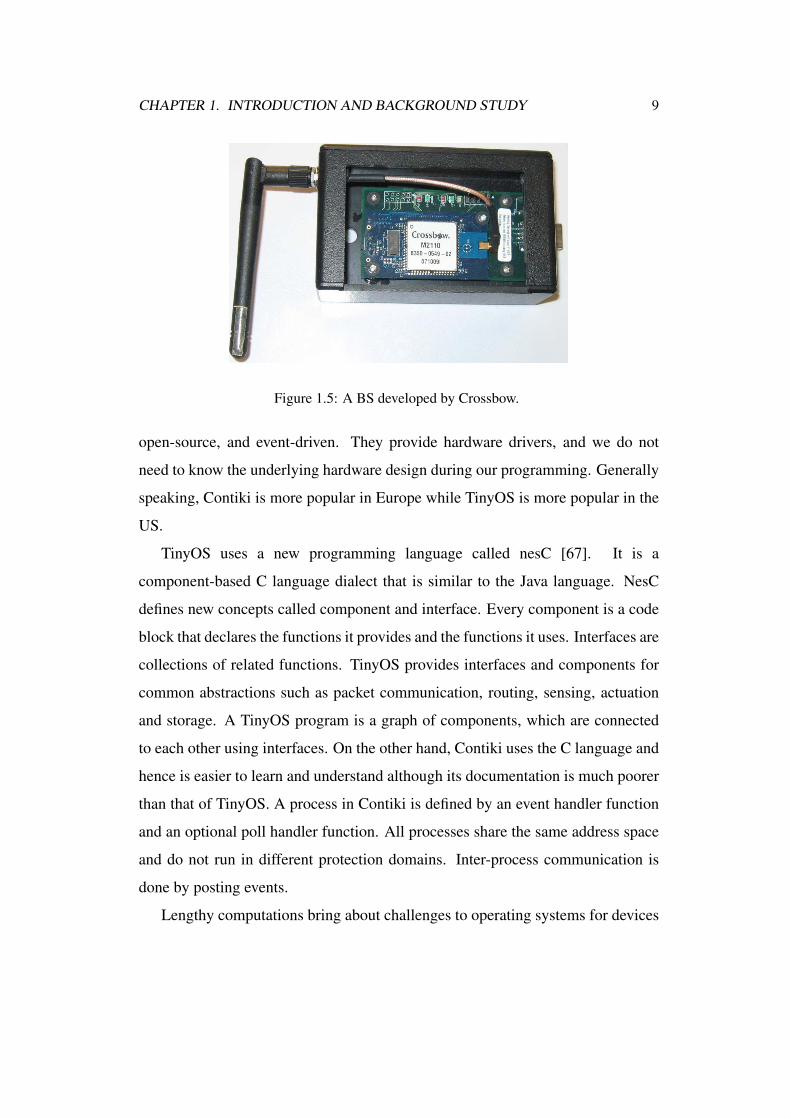
1.1.2 The Base Station (BS)
The BS is a centralized station, either fixed or mobile, that gets all the data
collected by the WSN. It can then analyze the data and show the results to the
application users. A WSN is usually equipped with one BS although it can be
allocated with several BSs. A BS should be able to communicate with the sensor
nodes in a WSN. It can be a PC or a sensor node with more powerful abilities
as shown in Figure 1.5 [1]. Any one of the previously described sensor nodes
can function as a BS when it is connected to a standard PC interface. We usually
connect a sensor node with a PC through a serial port.
1.1.3 The Operating System (OS) of the Sensor Node
As the vital component of the sensor node software, the operating system (OS)
manages the hardware resources and provides services for the applications. Since
the sensor nodes are resource-limited, the designed OS should be lightweight.
Although many operating systems are designed [17] [22] [33] [69], the most
popular two are Contiki [33] and TinyOS [49] [69], both of which are small, free,
CHAPTER 1. INTRODUCTION AND BACKGROUND STUDY 9
Figure 1.5: A BS developed by Crossbow.
open-source, and event-driven. They provide hardware drivers, and we do not
need to know the underlying hardware design during our programming. Generally
speaking, Contiki is more popular in Europe while TinyOS is more popular in the
US.
TinyOS uses a new programming language called nesC [67]. It is a
component-based C language dialect that is similar to the Java language. NesC
defines new concepts called component and interface. Every component is a code
block that declares the functions it provides and the functions it uses. Interfaces are
collections of related functions. TinyOS provides interfaces and components for
common abstractions such as packet communication, routing, sensing, actuation
and storage. A TinyOS program is a graph of components, which are connected
to each other using interfaces. On the other hand, Contiki uses the C language and
hence is easier to learn and understand although its documentation is much poorer
than that of TinyOS. A process in Contiki is defined by an event handler function
and an optional poll handler function. All processes share the same address space
and do not run in different protection domains. Inter-process communication is
done by posting events.
Lengthy computations bring about challenges to operating systems for devices

CHAPTER 1. INTRODUCTION AND BACKGROUND STUDY 10
that are resource-limited. For example, the lengthy computation required for
cryptographic operations typically takes several seconds to complete on CPU
constrained platforms [110]. In a purely event-driven operating system a lengthy
computation completely monopolizes the CPU, making the system unable to
respond to external events. To support computation that lasts very long time,
TinyOS requires programmers to divide the computation into many tasks, which
are similar to an interrupt handler. When a TinyOS component executes the
large computation, it posts tasks, which the OS will schedule to run later. Tasks
are non-preemptive and run in a FIFO (First In, First Out) order. Interrupts
can preempt the tasks. Hence, interrupts will not be greatly delayed by large
computations and can be responded in real-time. Instead of the multi-tasking
mechanism in TinyOS, Contiki allows lengthy computations to be preempted by
supporting preemptive multi-threading, which is implemented several years after
TinyOS was developed [62]. Preemptive multi-threading can be applied on a
per-process basis. It is implemented as an application library that is optionally
linked only with programs that explicitly require multi-threading.
Since the simulator allows algorithm development, system behavior study
and interaction observations, it can simplify the software development for sensor
networks under the specified OS [85]. We compare the simulators of TinyOS
and Contiki because they would affect the users’ preference in using an OS. As
a discrete event simulator and emulator of TinyOS, TOSSIM [68] simulates the
execution of nesC code on TinyOS. It allows emulation of actual hardware by
mapping hardware interruptions to discrete events. A simulated radio model is also
provided. By only replacing a few low-level TinyOS systems that touch hardware,
it can capture sensor node behavior at a very fine grain, allowing a wide range
of experimentation. Compiling unchanged TinyOS applications directly into its
framework, TOSSIM can simulate thousands of sensor nodes running complete
applications.

CHAPTER 1. INTRODUCTION AND BACKGROUND STUDY 11
The simulator developed in Contiki is Cooja [85]. It can also simulate
large-scale WSNs. The difference is that it allows cross-level simulation among
different types of sensor nodes: simultaneous simulation at many levels of the
system among different types of sensor nodes. COOJA combines low-level
simulation of sensor node hardware and simulation of high-level behavior in a
single simulation. COOJA currently is able to execute Contiki programs in two
different ways. Either by running the program code as compiled native code
directly on the host CPU (high-level), or by running compiled program code in
an instruction-level TI MSP430 emulator (low-level). For example, it can emulate
several TelosB sensor nodes at the low-level and several Contiki sensor nodes at
the high-level. COOJA is also able to simulate non-Contiki sensor nodes, such
as sensor nodes running another operating system. It is so user-friendly that it is
ported to support TinyOS simulation [38].
1.1.4 The Protocol Design of WSNs
Well-designed protocols can be integrated into the OS. Since the WSNs are
different from the other existing networks, such as wireless ad-hoc networks and
Internet, their protocols should be distinctive. The protocols in WSNs are mainly
composed of communication protocols which range from the physical layer to the
application layer. Other related protocols include coverage algorithms, localization
approaches, reprogramming protocols, security mechanisms and so on.
• To design physical layer protocols that suit WSNs, Wang et al. [120] and
Schurgers [103] et al. discuss energy efficient modulation for WSNs. Shih
et al. [107] present a hardware model for sensor node and then introduce the
design of physical layer aware protocols, algorithms, and applications that
minimize energy consumption of the systems.
• The medium access control (MAC) protocol design is one of the most active
research areas for WSNs. To save the energy consumption, most of the

CHAPTER 1. INTRODUCTION AND BACKGROUND STUDY 12
MAC protocols try to make the sensor nodes sleep as long as possible
while maintaining the normal communications, such as S-MAC [133] and
T-MAC [29]. S-MAC is a single-frequency contention-based protocol that
introduces periodic listening and sleeping mechanism. Its long time of
sleep greatly saves energy. However, this mechanism requires periodic
broadcast of synchronization frames to establish the sleep-wake up schedule.
In addition, sleep results in latency. The smaller the duty cycle (the
listening time divided by a period), the longer the latency, and the more the
energy that will be saved. There is a tradeoff between latency and energy.
T-MAC is proposed to enhance the poor results of the S-MAC protocol
under variable traffic loads. In T-MAC, the listening period ends when no
activation event has occurred for a time threshold TA. Although T-MAC
gives better results under these variable loads, its early sleeping leads to
longer latency. The above MAC protocols are synchronized approaches.
Degesys et al. [30] propose Desync-TDMA: a MAC protocol which does
not need synchronization. Desync-TDMA addresses two weaknesses of
traditional TDMA: it does not require a global clock and it automatically
adjusts to the number of participating sensor nodes, so that the bandwidth is
always fully utilized. In addition, a multi-channel MAC protocol based on
a light-weight channel hopping mechanism [60] is proposed and actually
implemented on commonly available sensor hardware. X-MAC [20],
BMAC [88], and WiseMAC [36] do not require synchronization, either.
They rely on preamble sampling to link together a sender with a receiver
who is duty cycling. Within them, the most popular one is X-MAC [20].
It allows sensor node sleeping, and it does not require the other methods
to wake up the sleeping receiver, such as a low-power radio equipment that
can be waken by short tones [114]. When a sender has data, the sender
transmits a preamble that is at least as long as the sleep period of the

CHAPTER 1. INTRODUCTION AND BACKGROUND STUDY 13
receiver. The receiver will wake up, detect the preamble, and stay awake
to receive the data. This allows low power communication without the
need of explicit synchronization between the sensor nodes. The receiver
only wakes for a short time to sample the medium, thereby limiting idle
listening. Finally, Halkes et al. proposes a hybrid MAC protocol combine
the synchronized protocol T-MAC with an asynchronous low power listening
MAC protocol [46].
• Synchronization (short for time synchronization) is closely related to the
MAC protocol design. It is an important feature of almost any distributed
systems. It enables data consistency and coordination in WSNs. Elson et
al. [37] argue that time synchronization schemes developed for traditional
networks are ill-suited for WSNs and suggest more appropriate approaches.
Maroti et al. [80] describe the Flooding Time Synchronization Protocol
(FTSP), especially tailored for applications requiring stringent precision on
resource limited wireless platforms. The proposed time synchronization
protocol uses low communication bandwidth and it is robust against node and
link failures. The FTSP achieves its robustness by utilizing periodic flooding
of synchronization messages and implicit dynamic topology updates. The
unique high precision performance is reached by utilizing MAC-layer time
stamping and comprehensive error compensation including clock skew
estimation. The FTSP was implemented on the Mica2 platform and
evaluated in a 60-node, multi-hop setup. Yoon et al. [134] propose another
time synchronization protocol especially relevant to sensor networks. The
performance of the protocol is also validated on a realistic testbed.
• Besides the MAC protocol design, the network protocol design is another
hot research topic in WSNs. To address the scalability and energy-efficiency
problems in WSNs, various routing protocols are designed to achieve
energy-efficient and robust multi-hop communications. Almost all of the

CHAPTER 1. INTRODUCTION AND BACKGROUND STUDY 14
routing protocols can be classified according to the network structure as flat,
hierarchical, or location-based [12]. In flat networks, all sensor nodes play
the same role while hierarchical protocols aim at clustering the sensor nodes
so that cluster heads can do some aggregation and reduction of data in order
to save energy. Location-based protocols utilize the position information
to relay the data to the desired regions rather than the whole network.
Directed diffusion is a flat routing protocol [51]. It is data-centric (DC)
and application-aware in the sense that all data generated by sensor nodes
is named by attribute-value pairs. The BS requests data by broadcasting
interests. Interest describes a task required to be done by the network.
Interest diffuses through the network hop-by-hop, and is broadcast by each
node to its neighbors. As the interest is propagated throughout the network,
gradients are setup to draw data satisfying the query towards the requesting
node, i.e., the BS. Each sensor node that receives the interest setups a
gradient toward the sensor nodes from which it receives the interest. This
process continues until gradients are setup from the sources back to the BS.
The intermediate sensor nodes can perform data aggregation in-network and
hence save the energy consumption. LEACH is a two-layer hierarchical
routing where one layer (sensor nodes in a cluster) is used to select cluster
heads and the other layer (sensor nodes that are cluster heads) is used for
routing [47]. Higher energy sensor nodes are selected as cluster heads that
are used to process and send the information the BS while low energy sensor
nodes are used to perform the sensing in the proximity of the target. By
performing data aggregation and fusion in order to decrease the number
of transmitted messages to the BS, the cluster head lowers the energy
consumption within a cluster. Geographic routing is a location-based routing
scheme in WSNs [124]. Unlike IP networks, communications on sensor
networks often directly use physical locations as addresses. For example,

CHAPTER 1. INTRODUCTION AND BACKGROUND STUDY 15
instead of querying a sensor with a particular ID, a user often queries
a geographic region. The identities of sensor nodes that happen to be
located in that region are not important. Any node in that region which
receives the query may participate in data aggregation and report the result
back to the user. Due to this location-centric communication paradigm of
sensor networks, geographic routing can be performed without incurring the
overhead of location directory services [71].
• The essential task of a transport layer protocol in WSNs is congestion control
(or reliability guarantee) [94]. CODA [119] provides congestion control
mechanisms to control the data stream to the BS. To do so, it introduces three
schemes: congestion detection, open-loop hop-by-hop back-pressure, and
closed-loop end-to-end multi-source regulation. CODA senses congestion
by checking each sensor node’s buffer occupancy and wireless channel load.
If they exceed a predefined threshold value, a sensor node will notify its
neighbor source node(s) to decrease the sending rate through an open-loop
hop-by-hop backpressure. Receiving a back-pressure signal, the neighbor
sensor nodes simply decrease the packet sending rate and also replay the
back-pressure continuously. Similarly, Bret et al. provides hop-by-hop
flow control, rate limiting of source traffic in the transit sensor nodes to
provide fairness and a prioritized MAC protocol [19]. POWER-SPEED
is a specifically tailored data transport protocol for WSNs to achieve
energy-efficient data transport for delay-sensitive event reporting [136]. In
POWER-SPEED, based on the spatio-temporal historic data of the upstream
QoS condition, sensor nodes select the next-hop neighbor, which completely
avoids control packets and improves the reliability in real-time applications.
With an adaptive transmitter power control scheme, POWER-SPEED
conveys packets in an energy-efficient manner while maintaining soft
real-time packet transport. As a real implementation of the transport layer

CHAPTER 1. INTRODUCTION AND BACKGROUND STUDY 16
protocol in WSNs, µ TCP/IP proposed in [35] and [34] modify the TCP/IP
protocol suite to make it viable for WSNs and provides similar transport
layer control for WSNs as that for the Internet.
• Although data aggregation is enabled by the routing mechanisms, it is done
at the application layer, such as data aggregation in clusters [112] and online
compression of data streams [109] in the application layer. Data aggregation
in networks is very efficient in performance improvement. It greatly reduces
the amount of data to be transmitted and contributes a lot to energy saving in
WSNs. Because sensed data in Wireless Sensor Networks (WSNs) reflect the
spatial and temporal correlations of physical attributes existing intrinsically
in the environment, sensor readings from neighboring sensor nodes in a
certain interval can be aggregated into one reading. Sunhee et al. [112]
propose the Clustered AGgregation (CAG) algorithm that forms clusters
of sensor nodes sensing similar values within a given threshold (spatial
correlation), and these clusters remain unchanged as long as the sensor values
stay within a threshold over time (temporal correlation). With CAG, only one
sensor reading per cluster is transmitted. In addition, CAG provides energy
efficient and approximate aggregation results with small and often negligible
and bounded errors. Soroush et al. tackle the problem of online compression
of data streams in the resource-constrained WSNs, where the traditional data
compression techniques cannot apply. They employ fast piecewise linear
approximation (PLA) methods with quality guarantee on data aggregation.
Other interesting applications include a energy usage monitor and a tiny web
service [111] [93]. LEAP2 platform [111] is a new embedded networked
sensor platform architecture that combines hardware and software tools to
provide detailed, fine-grained real-time energy usage information. With this
energy information system, 60% energy saving can be archived by carefully
selecting the system operating points. A tiny web service is proposed to

CHAPTER 1. INTRODUCTION AND BACKGROUND STUDY 17
enable an evolutionary sensornet system where additional sensor nodes may
be added after the initial deployment [93].
• Sensing coverage tells us how well each point in the region is covered
by the WSN. Network connectivity measures how reliably the information
gathered by the sensor nodes can be transmitted. Maintaining sufficient
sensing coverage and network connectivity with the minimum number of
active sensor nodes helps improving the reliability and performance in sensor
networks [41]. Wang et al. present the design and analysis of a novel
coverage configuration protocol (CCP) that can dynamically configures a
network to provide different feasible degrees of sensing coverage while
maintaining network connectivity [122]. The basic idea in CCP is that
each sensor maintains state information and checks eligibility criteria by
exchanging messages with its neighbors in order to decide whether or not
to turn itself off. Similarly, Wu et al. propose several local solutions that put
as many sensor nodes as possible to sleep for energy saving purposes, while
meeting different connectivity requirements [123].
• The data collected by the WSN are meaningless without knowing the
location from where the data are obtained. For example, if a fire breakout
is detected, it is critical to know where this event happened so that the
proper actions can be taken. Since most emerging applications based
on networked sensor nodes require location awareness to assist their
operations, such as annotating sensed data with location context, it is an
indispensable requirement for a sensor node to be able to find its own
location [79]. Currently, due to the limited-resource and some environments
not accessible by GPS, it is not feasible to use Global Positioning System
(GPS) hardware for this purpose. GPS-free solutions are favorable for the
location problem in WSNs. Sensor network localization algorithms estimate
the locations of sensor nodes with initially unknown location information

CHAPTER 1. INTRODUCTION AND BACKGROUND STUDY 18
by using knowledge of the absolute positions of a few sensor nodes and
inter-sensor measurements such as distance and bearing measurements. They
are classified into three categories: angle-of-arrival (AOA) measurements,
distance related measurements and received signal strength (RSS) profiling
techniques. The accuracy of AOA measurements is limited by the directivity
of the antenna, by shadowing and by multi-path reflections. Since the
antenna of a sensor node is not directed, this AOA-based method is not
favored in WSNs. As a distance-based localization method, a distributed
multidimensional scaling (MDS) method is proposed. It uses dimensionality
reduction techniques to estimate sensor node coordinates in two (or three)
dimensional space [53]. Relying on the RSS characteristics, Ray et al take
the probabilistic nature of indoor RF (radio frequency) signals into account
through the full set of probability distributions of signal characteristics as
seen by the cluster heads conditional on the position of the sensor [96].
Using these conditional probability distributions, they pose the location
detection problem as a hypothesis testing problem. Then they discretize the
space of possible sensor locations and seek to map the actual locations of
sensors onto this discrete set.
• WSNs need an efficient and reliable reprogramming service to facilitate
management and maintenance tasks [121]. For example, when bugs are
found after deployment, the WSN needs to update the application with
new code. How to disseminate the code efficiently without degrading the
performance of the WSN is very critical in maintaining the applications.
Traditional ways of manually reprogramming sensor nodes are costly, labor
intensive or even impossible since each node has to be collected from the
field and physically attached to a computer to install new codes. As a result,
reprogramming protocols should be enabled to facilitate code dissemination.
Trickle [70] is an algorithm for propagating and maintaining code updates

CHAPTER 1. INTRODUCTION AND BACKGROUND STUDY 19
in WSNs. In Trickle, sensor nodes stay up-to-date by occasionally
broadcasting a code summary to their neighbors. Its key contribution is the
use of suppression and dynamic adjustment of the broadcast rate to limit
transmissions among neighboring sensor nodes. A node suppresses its own
broadcast if it recently overhears a similar code summary. When sensor
nodes are not up-to-date, the broadcast rate is reduced, but is otherwise
increased up to a specified limit. These techniques allow Trickle to scale to
thousand-fold changes in network density, disseminate updates quickly, and
consume minimal resources in the quiescent state. While Trickle addresses
single packet dissemination, Deluge extends it to support large data objects
dissemination protocol from one or more source sensor nodes to many other
sensor nodes over a multi-hop WSN [50]. Specifically, It considers the
propagation of complete binary images. MNP also provides a multi-hop
reprogramming service [6]. To reduce the problem of collision and hidden
terminal problem, it proposes a sender selection algorithm that attempts to
guarantee that in a neighborhood there is at most one source transmitting the
program at a time. Jeong et al. design the Rsync algorithm to generate the
difference of the two program images, which allows distributing just the key
changes of the program [52]. This reprogramming is fast because it only
requires transmitting the incremental changes for the new program version.
• Security problems also exist in WSNs as in other systems. Due to the
distributed and ad-hoc nature of WSNs and no supervision after their
deployment, WSNs are vulnerable to numerous security threats that can
adversely affect their proper functioning [104]. The resource constraints in
the sensor nodes make traditional security mechanisms with large overhead
of computation and communication infeasible in WSNs. Because Elliptic
Curve Cryptography (ECC) offers a moderate security with a much smaller
key size, it is employed by Malan et al. to provide cryptography service for
CHAPTER 1. INTRODUCTION AND BACKGROUND STUDY 20
Mica2 sensor nodes in WSNs [78]. Zhu et al propose a localized encryption
and authentication protocol (LEAP), a key management protocol for WSNs
based on symmetric key algorithms LEAP [138]. It uses different keying
mechanisms for different packets depending on their security requirements.
Besides cryptography, various methods of defending against DoS attacks,
secure broadcasting mechanisms, secure routing mechanisms, sensor privacy
schemes, network intrusion detection mechanisms, secure data aggregation
techniques, and trust management schemes for WSN security are all worth
investigation.
1.2 Thesis Scope and Contributions
WSN applications are the target of many research efforts in WSNs. Suppose the
proper WSN hardware is given, then to provide such applications, researchers first
need to design the protocols that can be employed in WSNs. After implementing
the protocols, the researchers should test and verify the protocols so as to eliminate
as many problems as possible. By then, the WSN applications can be deployed in
the real field. Nevertheless, the after-deployment maintenance is very crucial for
keeping the WSN applications run normally. The whole process is shown is Figure
1.6. This thesis falls in three areas of WSNs in the process, namely, protocol
design, system testing, and application diagnosis, to obtain dependable WSNs.
Specifically, the work in this thesis is shown in the shadowed block in Figure 1.6.
1.2.1 Protocol Design
Protocol design is the beginning step of WSN application development. As
discussed previously, protocols of different layers and for different purposes need
to be proposed to fit the WSN applications. In terms of protocol design, this thesis
proposes an efficient MAC protocol and a reliable MAC protocol for underwater

CHAPTER 1. INTRODUCTION AND BACKGROUND STUDY 21
Software
Design
System
Testing
Application
Maintenance
Implement
software
Deploy
application
MAC layer
protocol
Network
layer protocol
Network
layer protocol
Application
layer protocol
Application
layer protocol
…… SimulationSimulation
Protocol
testing
TestbedTestbed
……
Protocol
diagnosis
……
Program
update
Program
update
Figure 1.6: The development, deployment, and maintenance of the WSN applications.
acoustic sensor networks (UWASNs), a type of WSNs that are deployed in the
water, especially in the oceans.
Due to the different transmission medium used in the water by UWASNs,
the efficiency of UWASNs is inferior to that of the terrestrial wireless sensor
networks (TWSNs). Moreover, the unreliability problem in UWASNs caused by
the packet loss is seldom considered. In improving the efficiency, we first identify
that the scheduling problem of UWASNs is very different from that of TWSNs.
After the scheduling problem analysis, we propose a protocol called RAS (routing
and application based scheduling protocol), a priority scheduling approach for
multi-hop topologies. RAS performs parallel transmissions and prioritizes the
scheduling by allocating longer time to heavier-traffic sensor nodes. Such priority
mechanism also benefits the fairness. Then we design a reliable RAS called RRAS
that obtains a tradeoff between the reliability and the efficiency. RRAS designs an
ACK (acknowledgement) and retransmission mechanism that is different from the
traditional one, so that it can maintain a comparable throughput while improving

CHAPTER 1. INTRODUCTION AND BACKGROUND STUDY 22
the reliability. On one hand, the ACK and retransmission do not follow the
data loss immediately. On the other hand, though distributed, the retransmission
mechanism is based on ALOHA, a random medium access method which is first
used in a wireless network in the 1970s. Extensive evaluations are conducted
to verify that RAS is efficient and RRAS achieves a tradeoff on reliability and
efficiency.
1.2.2 Protocol Testing
Protocol conformance testing is indispensable in preventing bugs from
sneaking into real deployments. It is especially important for WSNs whose
after-deployment fixing is very expensive [121]. Experiences from real WSN
deployments show that protocol implementations in sensor nodes are susceptible
to software failures, which may cause network failures or even breakdown.
Unfortunately, existing solutions with simulators cannot test the exact hardware
and implementation environment as real sensor nodes, whereas testbeds are
limited to small-scale networks and topologies. Furthermore, large-scale real
deployment is too expensive. To solve the problem, in this thesis, we present
RealProct (reliable Protocol conformance testing with Real sensor nodes), a
novel and reliable framework for testing protocol implementations against their
specifications in WSNs. Utilizing real sensor nodes in protocol conformance
testing, RealProct can ensure that the testing environment is as close to the real
deployment as possible. To save the hardware cost and control efforts required
by large-scale real deployments, RealProct virtualizes a large network with any
topology and generates non-deterministic events using only a small number of
sensor nodes. The framework is carefully designed to support efficient testing in
resource-limited sensor nodes. Moreover, test execution and verdict are optimized
to minimize the number of runs, while guaranteeing satisfactory false positive and
false negative rates. We implement RealProct and test it with the µIP TCP/IP

CHAPTER 1. INTRODUCTION AND BACKGROUND STUDY 23
protocol stack and a routing protocol developed for WSNs in Contiki-2.4. The
results demonstrate the effectiveness of RealProct by detecting several new bugs
and all previously discovered bugs in various versions of the µIP TCP/IP protocol
stack.
1.2.3 Protocol Diagnosis
Real-time diagnosing the WSN can help detecting failures in the WSN protocols
after deployment, thus facilitating the maintenance. Nevertheless, current
in-situ diagnosis methods are either intrusive or inefficient, because they either
inject diagnosis agents into each sensor node or build up another network for
diagnosis purpose. In this thesis, to attack these issues, we propose MDiag,
a Mobility-assisted Diagnosis approach that employs smartphones to patrol the
WSNs and diagnose failures. Diagnosing with a smartphone which is not a
component of WSNs does not intrude the execution of the WSNs. Moreover,
patrolling the smartphone in the WSNs to investigate failures is more efficient
than deploying another diagnosis network. During the patrol, packets are collected
and then analyzed by our implemented packet decoder. Statistical rules are also
designed to guide the detection of abnormal cases. Aiming at improving the
patrol efficiency, a patrol approach MSEP (maximum snooping efficiency patrol)
is proposed. Experiments with real sensor nodes and emulations statistically
demonstrate that MSEP is better than the naive method, greedy method, and
baseline method in increasing the detection rate and reducing the patrol time.
1.3 Thesis Organization
The rest of this thesis is organized as follows. In Chapter 2 [127], we investigate
how to design an efficient MAC protocol for WSNs, based on which we propose
a reliable MAC protocol for WSNs in Chapter 3 [128]. Chapter 4 discusses
the framework and techniques developed for protocol conformance testing in

CHAPTER 1. INTRODUCTION AND BACKGROUND STUDY 24
WSNs [129]. Diagnosing the WSNs on demand in real-time to detect protocol
failures is inspected in Chapter 5, while Chapter 6 concludes this thesis.
2 End of chapter.
Chapter 2
An Efficient MAC Protocol Design
Underwater acoustic sensor networks (UWASNs) are composed of underwater
sensor nodes that use sound to transmit information collected in the ocean. Since
the sound speed is lower than radio wave, UWASNs suffer from much lower
throughput and higher delay compared with terrestrial wireless sensor networks
(TWSNs). Current methods manage to alleviate the bottleneck by replacing
mutual handshakes with reservation mechanisms that consume lower overhead.
However, their throughput improvement and delay reduction are very limited (e.g.,
the throughput is only 30% of the theoretical maximum for TLohi in 8-node
networks), and most of their analysis and simulations are based on single-hop
communication. In this work, we tackle the above challenges by proposing
a priority scheduling approach for multi-hop topologies. First, we find that
the scheduling problem of UWASNs is very different from that of TWSNs,
and analyze the shortest schedule for the whole UWASN. Then, we design an
efficient priority scheduling protocol at the MAC layer. Our approach performs
parallel transmissions and prioritizes the scheduling by allocating longer time to
heavier-traffic nodes. We have conducted extensive evaluations which show that
the proposed protocol not only improves the throughput and delay performance
greatly, but also benefits the fairness.
25

CHAPTER 2. AN EFFICIENT MAC PROTOCOL DESIGN 26
Sender
Receiver
DATATt = 80ms
Time(ms)
RTS8ms
(b) A DATA transmission in UWASNs
Sender
Receiver
DATATt = 80ms
Time(ms)CTS8ms
RTS8ms
ACK8ms
(a) A DATA transmission in TWSNs
Tp = 3.7us, it is too small to be indicated in the figure
ACK8ms
Tp = 740ms
CTS8ms
Figure 2.1: A data transaction process.
2.1 Introduction
Ocean exploitation started from decades ago [108]. However, newer and more
efficient methods to explore the ocean, such as underwater acoustic sensor
networks (UWASNs) [11], only emerged recently. UWASNs play an important
role in ocean applications, such as oceanographic data collection, pollution
monitoring, offshore exploration, disaster prevention, assisted navigation and
so on. While terrestrial sensor networks (TWSNs) are densely deployed, in
underwater, the deployment is deemed to be sparser, due to the high cost of
underwater sensor nodes [11]. UWASNs employ sound to perform wireless
communications in the ocean because of its low attenuation property in the
water [92]. In comparison, TWSNs use radio-frequency electromagnetic wave
to communicate in the air. The speed of sound in the water is 1.5km/s while that of
radio waves in the air is 300,000km/s. As a result, poor throughput and high delay
become the bottleneck of UWASNs.
As an example, Figure 2.1 demonstrates the bottleneck of UWASNs by
comparing with TWSNs in a data transaction process. The data transaction of

CHAPTER 2. AN EFFICIENT MAC PROTOCOL DESIGN 27
Table 2.1: Parameters for data transmissions.Parameter Value
Data Rate 10 kbps
Data Packet Size 100 bytes
Control Packet Size 10 bytes
Transmission Range (communication range) 1500 m
Interference Range 3500 m
Average Distance between Two Nodes 1110 m
Guard time 20 ms
Wireless model TwoRayGround
Table 2.2: Tt and Tp for TWSNs and UWASNs.
Tt Tp
TWSNs 80ms 3.7µs
UWASNs 80ms 740ms
UWASNs takes much longer time than that of TWSNs, and thus the throughput is
much lower. In Figure 2.1, parameters [131] in Table 2.1 are adopted, and both
TWSNs and UWASNs employ the CSMA/CA mechanism [7] to transmit a packet.
Then we calculate the data transmission time (Tt) and the propagation time (Tp) for
TWSNs and UWASNs. The results are shown in Table 2.2, in which Tp ≪ Tt for
TWSNs, and Tt ≪ Tp for UWASNs. The long Tp of UWASNs (740ms) amplify
the throughput and delay penalty of handshaking protocols [105], thus UWASNs
should not apply the CSMA/CA as TWSNs do.
Although the long propagation time Tp results in bottleneck in UWASNs, it
enables parallel data transmissions as long as there is no collision. It enables the
start of another data transaction before the end of current data transaction. In
this way, we can mitigate the bottleneck with priority scheduling protocol called

CHAPTER 2. AN EFFICIENT MAC PROTOCOL DESIGN 28
RAS (routing and application based scheduling protocol). We summarize our
contributions as follows:
(1) After distinguishing the scheduling problem of UWASNs with that of
TWSNs, we formulate the scheduling problem. Then we prove that the complexity
of the algorithm to solve such a problem is exponential.
(2) By parallel transmissions and utilizing the information from routing and
application layer, we design an efficient priority scheduling protocol at the MAC
layer of the base station (BS).
(3) Extensive evaluations are conducted to show that the proposed protocol not
only improves the throughput and delay performance in multi-hop networks, but
also enhances the fairness.
In the remainder of this chapter, Section 2.2 describes related work. Section
2.3 gives us an overview of the RAS protocol. Section 2.4 formulates and analyzes
the scheduling problem for UWASNs, and then Section 2.5 illustrates RAS.
Performance evaluations of RAS are provided in Section 2.6while conclusions are
made in Section 2.7.
2.2 Related Work
Recently, there are extensive research efforts focusing on improving the
performance of UWASNs by enhancing the traditional data transmission model
at the MAC layer. Slotted FAMA [82] is a handshaking-based protocol designed
to improve the traditional data transmission model and avoid collisions caused
by the hidden terminal problem. It synchronizes all nodes and makes all the
transmissions start at the beginning of a slot. The slot length is the sum of the
maximum propagation delay and the transmission time of a CTS packet. Although
it can efficiently avoid collision caused by the long propagation of UWASNs, its
throughput and delay performances are poor because the slot is too long. Our RAS
protocol does employ such long slot and its throughput and delay performances are

CHAPTER 2. AN EFFICIENT MAC PROTOCOL DESIGN 29
better.
Regarding the RTS/CTS handshaking transmission model in UWASNs as
inefficient, Chirdchoo et al. propose two aloha-based MAC protocols [26].
Although they do not use RTS/CTS handshake to avoid collisions, they
require nodes to broadcast their location information for calculating inter-node
propagation delays, which helps avoid collisions and enhances throughput. In
addition, Affan et al. develop T-Lohi [114] which uses short wake-up tones to
reserve channel for data transmission. It increases the throughput to 30% of the
theoretical optimal, but its node needs a low-power receiver that can be waken
by short tones. UW-FLASHR [131] is based on TDMA rather than RTS/CTS
handshaking. It divides its cycle into two portions: experimental portion and
DATA portion. In the experimental portion, control frames RTS and CTS for
requesting new transmission time slots within the DATA portion are exchanged.
In the DATA portion, nodes only transmit data in the already acquired time
slots. Every node has to obtain data transmission slots in an experimental portion
before its data transmission. With such reservation, it improves the throughput by
utilizing the long propagation delay. However, a node does not know whether its
required time slot would collide with other nodes’ schedules, and it may need to
try several times before establishing a successful time slot. In addition, even if a
node does not need to request a new time slot, it cannot save energy by getting
into the sleep state. Although our method is also based on TDMA, our scheduling
elements are different from the existing work.
2.3 RAS Overview
There are three practical network scenarios for UWASNs: static two-dimensional
UWASNs for ocean bottom monitoring, static three-dimensional UWASNs
for ocean column monitoring, and three-dimensional networks of autonomous
underwater vehicles [11]. In this chapter, we focus on the first scenario. For
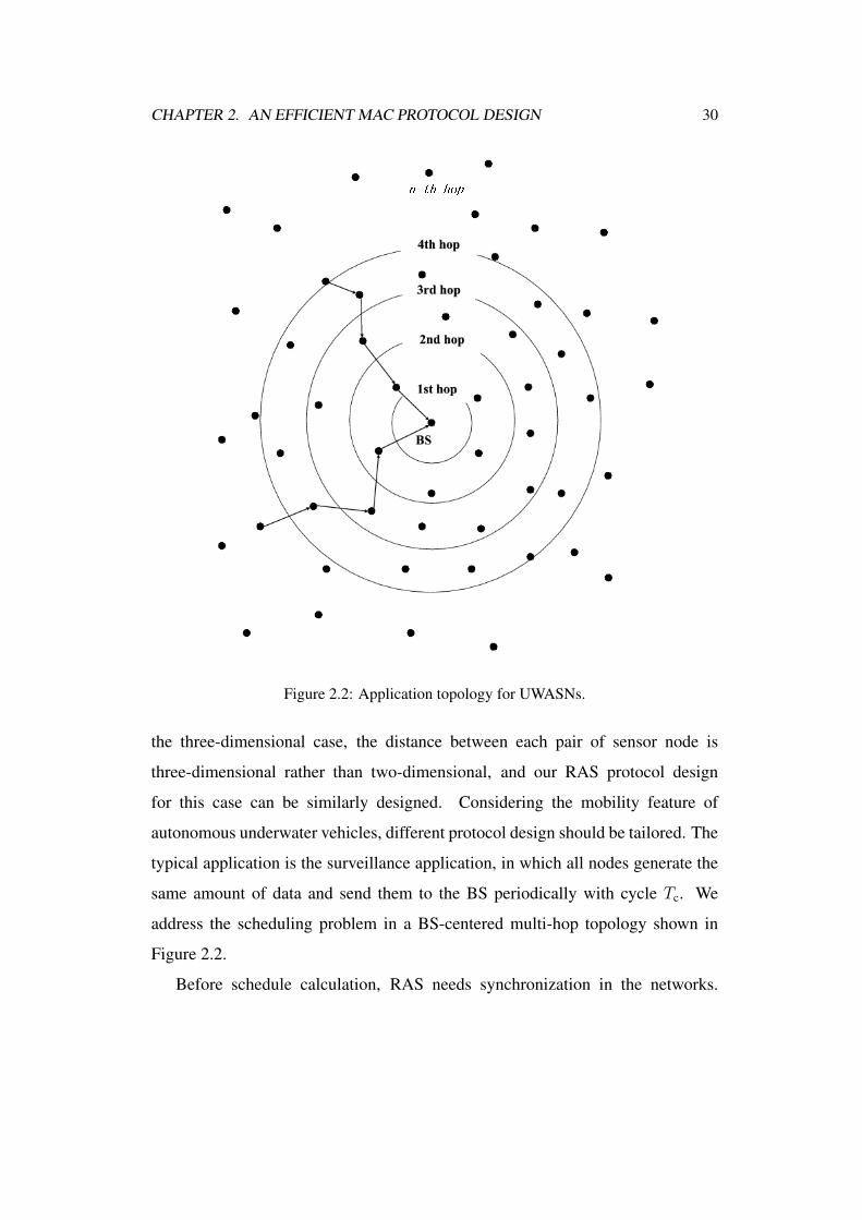
CHAPTER 2. AN EFFICIENT MAC PROTOCOL DESIGN 30
Figure 2.2: Application topology for UWASNs.
the three-dimensional case, the distance between each pair of sensor node is
three-dimensional rather than two-dimensional, and our RAS protocol design
for this case can be similarly designed. Considering the mobility feature of
autonomous underwater vehicles, different protocol design should be tailored. The
typical application is the surveillance application, in which all nodes generate the
same amount of data and send them to the BS periodically with cycle Tc. We
address the scheduling problem in a BS-centered multi-hop topology shown in
Figure 2.2.
Before schedule calculation, RAS needs synchronization in the networks.

CHAPTER 2. AN EFFICIENT MAC PROTOCOL DESIGN 31
Whole Period: Tc
Ts
Td Tg
Time Slot 1 Time Slot Time Slot
Ts
Sleeping Period
DATA transmission Period: Tw
Figure 2.3: RAS cycle.
Although there exists many synchronization methods [113], for the sake of
simplicity and low cost, RAS only requires coarse synchronization through the
initial packet exchange or the information piggybacked in the received packets
as [117] and [131] do. Meanwhile, it can calculate the rough propagation delays
between nodes by checking time stamps during the synchronization process [117].
With synchronization, the nodes can work and sleep periodically [133]. In Figure
2.3, the RAS cycle Tc is divided into two portions. One portion is the sleeping
period, and the other is the working period Tw which is divided into many time
slots Ts. One time slot is composed of Td, the time duration for transmitting a
DATA, and Tg, the guard time for avoiding collisions introduced by imprecise
synchronization and propagation time calculation. The actual value of Tg is
determined by the real deployment environment. If there is a data burst due to
abnormal events, nodes can transmit them in the following sleeping period by
notifying the related nodes in advance. In this way, data burst does not require
updates of the working schedule. In the future we focus on analyzing the working
schedule in one cycle.
Since the sensor nodes are anchored to the bottom of the ocean and are thus
static. It is practical to employ static routing because the networks are static.
In addition, the monitoring applications only require DATA transmissions from
the sensor nodes to the BS. Then the BS calculates the number of DATA to
be transmitted and received at each node. Finally, the BS can calculate for all
the sensor nodes the working schedule on when to send and receive DATA, and
CHAPTER 2. AN EFFICIENT MAC PROTOCOL DESIGN 32
broadcast the schedule to all the sensor nodes to follow for a long time. The steps
are shown in Algorithm 1.
Algorithm 1 RAS protocol at the BS (It runs at the initialization phase).1: Coarse synchronization through the initial packet exchange.
2: Calculate the rough propagation delay between nodes through the previous packet
exchange.
3: Calculate static routing.
4: Calculate the number of data to be transmitted and received at each node.
5: CalcSchedule() /*Algorithm 2*/.
6: The BS broadcasts the routing table and the schedule to all its children with high
power.
These processes cost little efforts because they do not require frequent updates.
Therefore, the major goal is how to make the working period of the whole network
as short as possible so as to save the energy and improve the network efficiency,
i.e., how to design an efficient schedule for the working period in a cycle.
2.3.1 Scheduling Element
Next, we show that the scheduling problem of UWASNs is different from that
of TWSNs because the scheduling elements of the former are more complex
than those of the latter. Since the purpose of scheduling is to arrange the
data transactions of all nodes, the scheduling element corresponds to one data
transaction. It consists of three time points: data transmission (DT) time, data
reception1 (DR) time, and a sequence of interference reception 2 (IR) time. For
example, in Figure 2.4, the scheduling element of node A’s first data transmission
to B is composed of DT1, DR1 and IR1. They occur at different time because Tp
in UWASNs is long enough (740ms) to distinguish them. In contrast, the three1reception of a packet destined for it.2reception of a packet not destined for it.
CHAPTER 2. AN EFFICIENT MAC PROTOCOL DESIGN 33
B
C
Time
A
Time
Time
DR stands for data receptionIR stands for interference reception
DT stands for data transmission
DT
1IR3IR2
DT
2
DR
1
DR
3
DT
3
DR
2IR1
Figure 2.4: Data transmissions among 3 nodes in UWASNs.
time points are the same in TWSNs because Tp in TWSNs is too small (3.7µs) to
differentiate them [99]. The different time values make the scheduling problem in
UWASNs very complicated. While in TWSNs we schedule each element in one
time slot, UWASNs’ scheduling element cannot be accommodated in one time
slot.
Due to Tt ≪ Tp in UWASNs, we can improve throughput and delay
performance by parallel transmission. Actually, nodes should transmit or receive
at any time as long as there are no collisions. In this way, channel idling is avoided,
thus throughput and delay performance can be enhanced. For example, in Figure
2.4, nodes B and C transmit packet 2 and packet 3 to each other simultaneously,
but their receptions are not collided. In this case, collisions will surely happen in
TWSNs. Specifically, node B does not have to postpone her packet 2 transmissions
until she has received packet 1 from node A. Many data transactions overlap
in time, and they all include interference IRs, but these IRs do not corrupt the
normal reception IRs. Thus, by scheduling these unique scheduling elements
logically to avoid collisions, throughput and delay performance can be greatly
improved. Hence, we need to answer how to schedule without collision and
improve throughput and delay performance.
CHAPTER 2. AN EFFICIENT MAC PROTOCOL DESIGN 34
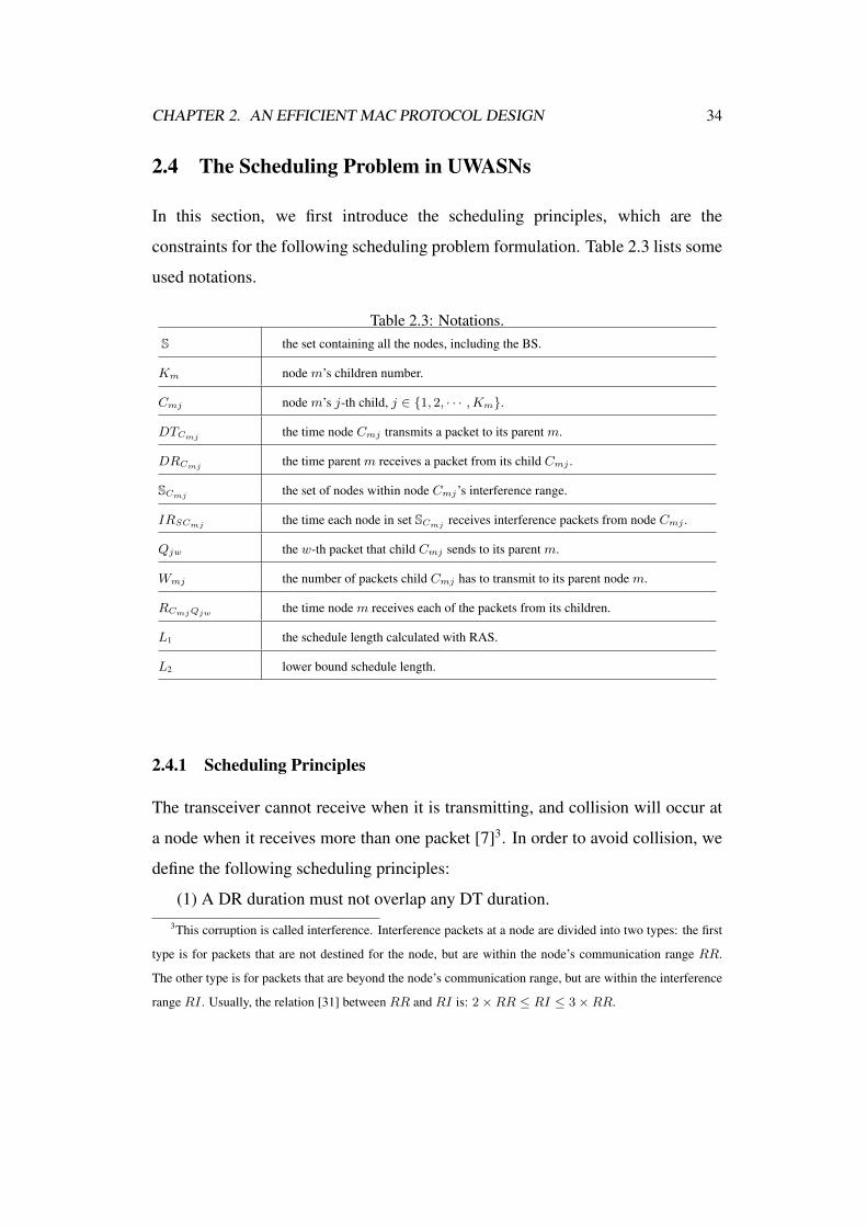
2.4 The Scheduling Problem in UWASNs
In this section, we first introduce the scheduling principles, which are the
constraints for the following scheduling problem formulation. Table 2.3 lists some
used notations.
Table 2.3: Notations.S the set containing all the nodes, including the BS.
Km node m’s children number.
Cmj node m’s j-th child, j ∈ {1, 2, · · · ,Km}.
DTCmj the time node Cmj transmits a packet to its parent m.
DRCmj the time parent m receives a packet from its child Cmj .
SCmj the set of nodes within node Cmj’s interference range.
IRSCmj the time each node in set SCmj receives interference packets from node Cmj .
Qjw the w-th packet that child Cmj sends to its parent m.
Wmj the number of packets child Cmj has to transmit to its parent node m.
RCmjQjw the time node m receives each of the packets from its children.
L1 the schedule length calculated with RAS.
L2 lower bound schedule length.
2.4.1 Scheduling Principles
The transceiver cannot receive when it is transmitting, and collision will occur at
a node when it receives more than one packet [7]3. In order to avoid collision, we
define the following scheduling principles:
(1) A DR duration must not overlap any DT duration.3This corruption is called interference. Interference packets at a node are divided into two types: the first
type is for packets that are not destined for the node, but are within the node’s communication range RR.
The other type is for packets that are beyond the node’s communication range, but are within the interference
range RI . Usually, the relation [31] between RR and RI is: 2×RR ≤ RI ≤ 3×RR.

CHAPTER 2. AN EFFICIENT MAC PROTOCOL DESIGN 35
(2) A DR duration must not overlap any IR duration.
(3) A DR duration must not overlap any other DR duration.
(4) Any other overlaps are allowed as long as they can happen. For example,
DT duration can overlap IR duration(s), IR duration can overlap IR duration(s).
Since there is no data from the BS to sensor nodes, we can design a compact
schedule by only allocating time for data from sensor nodes to the BS. Thus the
next principle is:
(5) No DR from i-th hop node to (i+ 1)-th hop node, and i represents the hop
number from the BS.
The goal of data transactions is to guarantee successful receptions, and we
arrive at the last principle:
(6) A node considers DR duration as the scheduling basis rather than DT or IR
duration.
With DR as the scheduling basis, we do not have to consider whether IR will
overlap other IRs and DTs. In addition, we can increase the throughput and reduce
delay by making nodes transmit or receive instead of idling whenever no DR is
overlapped.
2.4.2 Scheduling Problem Formulation
Under parallel transmissions, we aim at calculating the shortest working period
of a cycle within which all the nodes’ expected data are transmitted and received,
such that we can make the nodes sleep as the long as possible while finishing their
communication. We formulate this problem as follows.
Let S be the set containing all nodes, including the BS. Suppose node m has
Km nodes that send packets to it, so that node m is called a parent and the Km
nodes are called its children. Each child of m is denoted by Cmj . Node m has Km
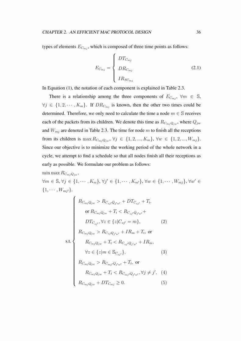
CHAPTER 2. AN EFFICIENT MAC PROTOCOL DESIGN 36
types of elements ECmj, which is composed of three time points as follows:
ECmj=
DTCmj
DRCmj
IRSCmj
(2.1)
In Equation (1), the notation of each component is explained in Table 2.3.
There is a relationship among the three components of ECmj, ∀m ∈ S,
∀j ∈ {1, 2, · · · , Km}. If DRCmjis known, then the other two times could be
determined. Therefore, we only need to calculate the time a node m ∈ S receives
each of the packets from its children. We denote this time as RCmjQjw, where Qjw
and Wmj are denoted in Table 2.3. The time for node m to finish all the receptions
from its children is maxRCmjQjw, ∀j ∈ {1, 2, ..., Km}, ∀w ∈ {1, 2, ...,Wmj}.
Since our objective is to minimize the working period of the whole network in a
cycle, we attempt to find a schedule so that all nodes finish all their receptions as
early as possible. We formulate our problem as follows:
minmaxRCmjQjw,
∀m ∈ S, ∀j ∈ {1, · · · , Km}, ∀j′ ∈ {1, · · · , Km′}, ∀w ∈ {1, · · · ,Wmj}, ∀w′ ∈
{1, · · · ,Wmj′}.
s.t.
RCmjQjw> RCzj′Qj′w′ +DTCzj′ + Tt,
or RCmjQjw+ Tt < RCzj′Qj′w′+
DTCzj′ , ∀z ∈ {z|Czj′ = m}, (2)
RCmjQjw> RCzjQj′w′ + IRm + Tt, or
RCmjQjw+ Tt < RCzj′Qj′w′ + IRm,
∀z ∈ {z|m ∈ SCzj′}, (3)
RCmjQjw> RCmj′Qj′w′ + Tt, or
RCmjQjw+ Tt < RCmj′Qj′w′ ,∀j ̸= j′, (4)
RCmjQjw+DTCmj
≥ 0. (5)
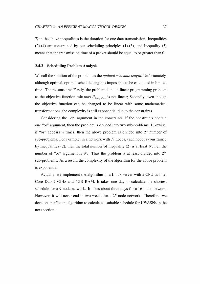
CHAPTER 2. AN EFFICIENT MAC PROTOCOL DESIGN 37
Tt in the above inequalities is the duration for one data transmission. Inequalities
(2)-(4) are constrained by our scheduling principles (1)-(3), and Inequality (5)
means that the transmission time of a packet should be equal to or greater than 0.
2.4.3 Scheduling Problem Analysis
We call the solution of the problem as the optimal schedule length. Unfortunately,
although optimal, optimal schedule length is impossible to be calculated in limited
time. The reasons are: Firstly, the problem is not a linear programming problem
as the objective function minmaxRCmjQjwis not linear; Secondly, even though
the objective function can be changed to be linear with some mathematical
transformations, the complexity is still exponential due to the constraints.
Considering the “or” argument in the constraints, if the constraints contain
one “or” argument, then the problem is divided into two sub-problems. Likewise,
if “or” appears n times, then the above problem is divided into 2n number of
sub-problems. For example, in a network with N nodes, each node is constrained
by Inequalities (2), then the total number of inequality (2) is at least N , i.e., the
number of “or” argument is N . Thus the problem is at least divided into 2N
sub-problems. As a result, the complexity of the algorithm for the above problem
is exponential.
Actually, we implement the algorithm in a Linux server with a CPU as Intel
Core Duo 2.8GHz and 4GB RAM. It takes one day to calculate the shortest
schedule for a 9-node network. It takes about three days for a 16-node network.
However, it will never end in two weeks for a 25-node network. Therefore, we
develop an efficient algorithm to calculate a suitable schedule for UWASNs in the
next section.

CHAPTER 2. AN EFFICIENT MAC PROTOCOL DESIGN 38
2.5 RAS Protocol
The previous subsection proves that the scheduling elements are complex and it is
impractical to calculate the shortest schedule. Although minimizing the working
period in a cycle focuses on throughput improvement, it ignores the fairness and
queue length. In this section, we propose an efficient scheduling algorithm, a
routing and application based scheduling protocol RAS, to solve the formulated
scheduling problem with a near-optimal solution. According to the network
scenario in the overview section, it is practical for RAS to take advantage of the
routing information and only schedule data transmission from sensor nodes to the
BS. With them, RAS can calculate a compact schedule for data exchange under
the same scheduling principles.
2.5.1 Scheduling Algorithm of the RAS Protocol
We call the schedule length calculated with RAS as L1, and obviously the optimal
schedule length is less than L1. In RAS, the scheduling elements are shown in
Equation (1), and a transaction of data transmission and reception will last for
several time slots. According to scheduling principle (6), we will schedule all the
elements generated in a cycle equals by scheduling all the data receptions in a
cycle. Let Si = {m : node m is i hops from the BS, m ∈ S}. Assuming a node’s
distance from the BS is proportional to its hop distance to the BS, the following is
the priority scheduling steps of RAS algorithm:
Step1: Schedule the BS’s DR from 1-hop nodes.
Step2: Schedule the DR tier by tier: from inner tier to outer tier, i.e., from DR
of nodes in Si to DR of nodes in Si+1, i ∈ {1, 2, 3, · · · , H−1}, H is the maximum
hop distance to the BS.
Step3: For each node m ∈ Si that is going to receive data packets from
its children Cmj ∈ Si+1, j = 1, 2, ..., Km, arrange its DR from its children
alternatively. For example, node 1 has two children A and B. In a cycle, each
CHAPTER 2. AN EFFICIENT MAC PROTOCOL DESIGN 39
of them send 3 packets PAi, PBi to node 1, and i ∈ 1, 2, 3. Then one possible DR
sequence at node 1 is: PA1, PB1, PA2, PB2, PA3, PB3.
The reason to schedule the BS’s DR first is that the topmost goal is for the
BS to receive all the data generated by all other nodes in a cycle. The reason
to prioritize the inner tier nodes over the outer tier nodes is that the inner-tier
nodes are affording much heavier traffic. It is unfair for them to share the same
bandwidth with other light-traffic nodes. In addition, the packets forwarded by the
inner tier nodes are forwarded more hops than those forwarded by the outer tier
nodes. Colliding or dropping those packets would cost more efforts to retransmit.
Finally, to alternate the receptions among the children provides load balancing of
the nodes. If fairness is not considered for a parent’s children, a few children
might drop packets due to congestion whereas other children’s queues are far from
full. Therefore, when we alternate the children’s transmissions, we improve the
fairness. The three steps are shown in Algorithm 2. How RAS works at the sensor
nodes is shown in Algorithm 3.
2.5.2 Analysis of the RAS Protocol
Since the upper bound for the RAS schedule length (L1) can be infinitely long, we
only discuss L2, the lower bound for the schedule length. Assuming each node
generates P packets in a cycle, then the BS has to receive N × P packets in total
from 1-hop nodes in a N -node network. To receive packets, it has to wait for
at least the propagation time Tp of one packet. Therefore, the shortest time for
receiving all the N × P packets is N × P × Ts + Tp. We call this time period
L2 as the lower bound, which cannot be achieved in large-scale networks due to
interferences. L2 is the shortest time for the BS to finish all its receptions while
L1 is the time for all the nodes, including the BS, in a network to finish their
receptions. Therefore, L2 is no larger than L1. We can use L2 to indicate the lower
bound for L1 instead of using the optimal schedule length which is intractable.

CHAPTER 2. AN EFFICIENT MAC PROTOCOL DESIGN 40
Algorithm 2 CalcSchedule() function at the BS.1: Parent = BS; hop = 1. //schedule the BS’s DR from 1-hop nodes
2: while hop ≤ maxhop. do
3: while Parent has children. do
4: while Parent has data to receive from its children. do
5: if Parent is idle in the Time Slot Slot. then
6: With global information, Parent searches its entire children to alternatively
find a child whose transmission results in its reception at the Slot.
7: if Parent finds a suitable child. then
8: schedule the child’s transmission and the related reception and
interference.
9: break searching.
10: end if
11: end if
12: Parent fetches the next Slot for reception.
13: end while
14: fetch the next Parent to schedule reception.
15: end while
16: hop = hop + 1. //schedule the DR tier by tier
17: end while

CHAPTER 2. AN EFFICIENT MAC PROTOCOL DESIGN 41
Algorithm 3 RAS protocol at the other nodes (It runs at each sensor node after the
initialization).1: Node x receives routing information and a schedule from the BS.
2: Synchronization.
3: while 1 do
4: if node x is in sleeping period. then
5: sleep until working period starts.
6: end if
7: if abnormal events happen. then
8: request x’s parent to wait for data in sleeping period.
9: end if
10: if receive data from x’s children. then
11: receive the data as scheduled.
12: end if
13: if x has data to send. then
14: send the data in working period as scheduled.
15: end if
16: end while

CHAPTER 2. AN EFFICIENT MAC PROTOCOL DESIGN 42
2.6 Performance Evaluation
We conduct the performance evaluation in the popular freeware network simulator
ns-3 [3] with parameters shown in Table 2.1. Using the setdest tool of ns-3,
we generate network scenarios of the same node density with six different sizes:
from 9-node network to 64-node network. In those networks, nodes are randomly
distributed and connected without holes, and the maximum hop distance ranges
from 1 hop to 7 hops. For networks of each size, we calculate the performance
under about 10 different topologies and show the average results. We employ
the underlying and traditional propagation model of ns-3 after adjusting the
transmission medium parameters as [117] and [131] do. The reason of using
such propagation model is that although acoustic waves in water suffer significant
absorptive losses, scattering and refraction, those factors do not change the latency
relationship among DT, DR and IR.
In the following we first compare the schedule length of RAS with the lower
bound schedule length. Next we implement RAS and UW-FLASHR [131] in ns-3,
and compare their performance in terms of throughput, delay and fairness.
2.6.1 Schedule Length
In this subsection, we calculate the lower bound schedule length L2 and the RAS
schedule length L1 when the number of packets generated by each node in a cycle
varies from 1 to 10. We do not draw the lines for the optimal schedule length
because it is intractable in limited time.
In Figure 2.5, all the lines are almost linear, which means that RAS is scalable
in calculating the schedule no matter the traffic rate is low or high. Since the
schedule length is the working time under a certain traffic rate, the shorter it is, the
longer the time that the whole network could sleep for. The whole network could
increase their throughput by working in the sleeping period. Therefore, the shorter
the schedule length is, the higher the throughput could be. Observing the value
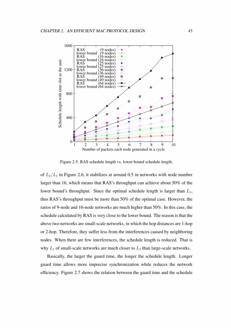
CHAPTER 2. AN EFFICIENT MAC PROTOCOL DESIGN 43
0
400
800
1200
1600
1 2 3 4 5 6 7 8 9 10
Sch
edule
len
gth
wit
h t
ime
slot
as t
he
unit
Number of packets each node generated in a cycle
RAS (9 nodes)lower bound (9 nodes)RAS (16 nodes)lower bound (16 nodes)RAS (25 nodes)lower bound (25 nodes)RAS (36 nodes)lower bound (36 nodes)RAS (49 nodes)lower bound (49 nodes)RAS (64 nodes)lower bound (64 nodes)
Figure 2.5: RAS schedule length vs. lower bound schedule length.
of L2/L1 in Figure 2.6, it stabilizes at around 0.5 in networks with node number
larger than 16, which means that RAS’s throughput can achieve about 50% of the
lower bound’s throughput. Since the optimal schedule length is larger than L1,
thus RAS’s throughput must be more than 50% of the optimal case. However, the
ratios of 9-node and 16-node networks are much higher than 50%. In this case, the
schedule calculated by RAS is very close to the lower bound. The reason is that the
above two networks are small-scale networks, in which the hop distances are 1-hop
or 2-hop. Therefore, they suffer less from the interferences caused by neighboring
nodes. When there are few interferences, the schedule length is reduced. That is
why L1 of small-scale networks are much closer to L2 than large-scale networks.
Basically, the larger the guard time, the longer the schedule length. Longer
guard time allows more imprecise synchronization while reduces the network
efficiency. Figure 2.7 shows the relation between the guard time and the schedule
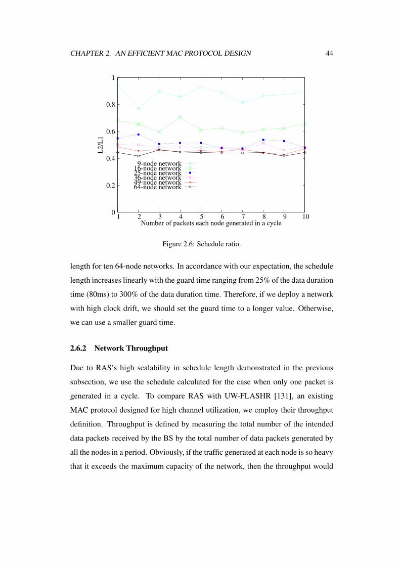
CHAPTER 2. AN EFFICIENT MAC PROTOCOL DESIGN 44
0
0.2
0.4
0.6
0.8
1
1 2 3 4 5 6 7 8 9 10
L2
/L1
Number of packets each node generated in a cycle
9-node network16-node network25-node network36-node network49-node network64-node network
Figure 2.6: Schedule ratio.
length for ten 64-node networks. In accordance with our expectation, the schedule
length increases linearly with the guard time ranging from 25% of the data duration
time (80ms) to 300% of the data duration time. Therefore, if we deploy a network
with high clock drift, we should set the guard time to a longer value. Otherwise,
we can use a smaller guard time.
2.6.2 Network Throughput
Due to RAS’s high scalability in schedule length demonstrated in the previous
subsection, we use the schedule calculated for the case when only one packet is
generated in a cycle. To compare RAS with UW-FLASHR [131], an existing
MAC protocol designed for high channel utilization, we employ their throughput
definition. Throughput is defined by measuring the total number of the intended
data packets received by the BS by the total number of data packets generated by
all the nodes in a period. Obviously, if the traffic generated at each node is so heavy
that it exceeds the maximum capacity of the network, then the throughput would
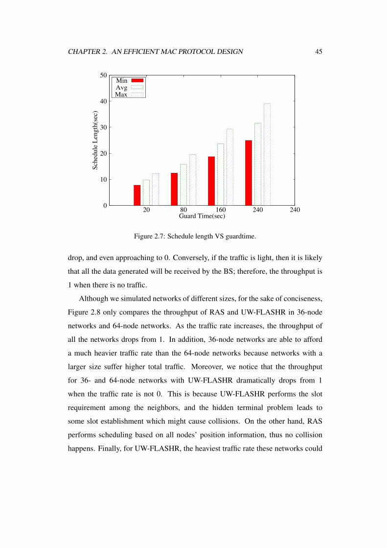
CHAPTER 2. AN EFFICIENT MAC PROTOCOL DESIGN 45
0
10
20
30
40
50
20 80 160 240 240
Sch
edu
le L
eng
th(s
ec)
Guard Time(sec)
Min Avg Max
Figure 2.7: Schedule length VS guardtime.
drop, and even approaching to 0. Conversely, if the traffic is light, then it is likely
that all the data generated will be received by the BS; therefore, the throughput is
1 when there is no traffic.
Although we simulated networks of different sizes, for the sake of conciseness,
Figure 2.8 only compares the throughput of RAS and UW-FLASHR in 36-node
networks and 64-node networks. As the traffic rate increases, the throughput of
all the networks drops from 1. In addition, 36-node networks are able to afford
a much heavier traffic rate than the 64-node networks because networks with a
larger size suffer higher total traffic. Moreover, we notice that the throughput
for 36- and 64-node networks with UW-FLASHR dramatically drops from 1
when the traffic rate is not 0. This is because UW-FLASHR performs the slot
requirement among the neighbors, and the hidden terminal problem leads to
some slot establishment which might cause collisions. On the other hand, RAS
performs scheduling based on all nodes’ position information, thus no collision
happens. Finally, for UW-FLASHR, the heaviest traffic rate these networks could
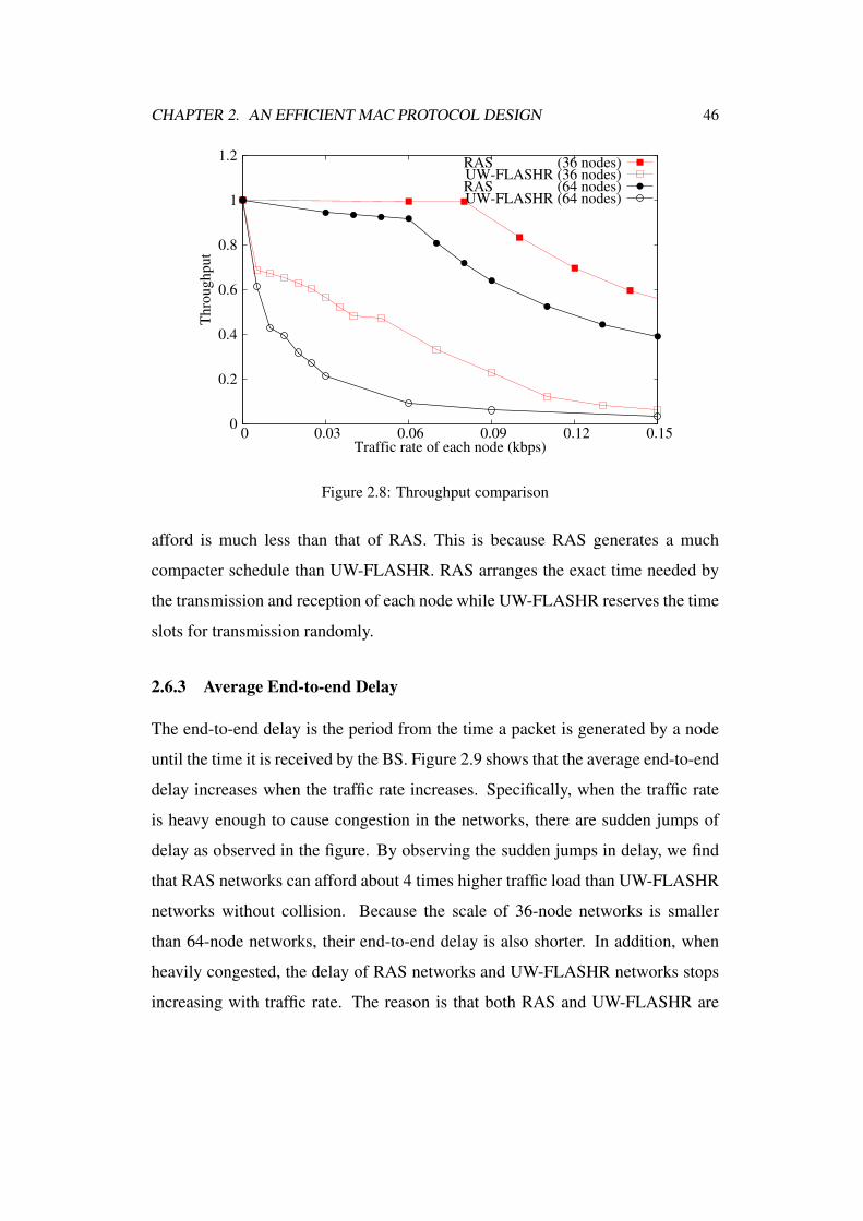
CHAPTER 2. AN EFFICIENT MAC PROTOCOL DESIGN 46
0
0.2
0.4
0.6
0.8
1
1.2
0 0.03 0.06 0.09 0.12 0.15
Th
rou
gh
pu
t
Traffic rate of each node (kbps)
RAS (36 nodes)UW-FLASHR (36 nodes)RAS (64 nodes)UW-FLASHR (64 nodes)
Figure 2.8: Throughput comparison
afford is much less than that of RAS. This is because RAS generates a much
compacter schedule than UW-FLASHR. RAS arranges the exact time needed by
the transmission and reception of each node while UW-FLASHR reserves the time
slots for transmission randomly.
2.6.3 Average End-to-end Delay
The end-to-end delay is the period from the time a packet is generated by a node
until the time it is received by the BS. Figure 2.9 shows that the average end-to-end
delay increases when the traffic rate increases. Specifically, when the traffic rate
is heavy enough to cause congestion in the networks, there are sudden jumps of
delay as observed in the figure. By observing the sudden jumps in delay, we find
that RAS networks can afford about 4 times higher traffic load than UW-FLASHR
networks without collision. Because the scale of 36-node networks is smaller
than 64-node networks, their end-to-end delay is also shorter. In addition, when
heavily congested, the delay of RAS networks and UW-FLASHR networks stops
increasing with traffic rate. The reason is that both RAS and UW-FLASHR are
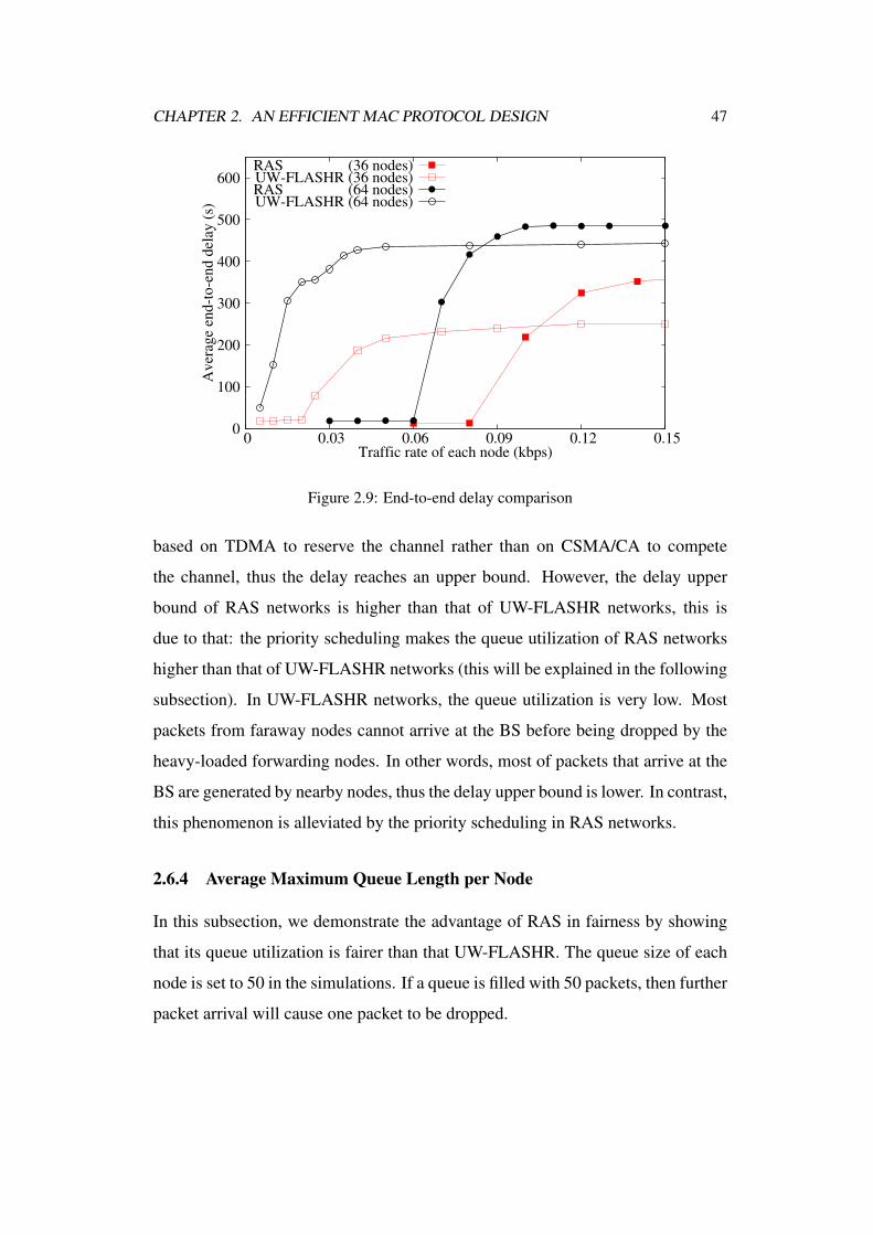
CHAPTER 2. AN EFFICIENT MAC PROTOCOL DESIGN 47
0
100
200
300
400
500
600
0 0.03 0.06 0.09 0.12 0.15
Av
erag
e en
d-t
o-e
nd
del
ay (
s)
Traffic rate of each node (kbps)
RAS (36 nodes)UW-FLASHR (36 nodes)RAS (64 nodes)UW-FLASHR (64 nodes)
Figure 2.9: End-to-end delay comparison
based on TDMA to reserve the channel rather than on CSMA/CA to compete
the channel, thus the delay reaches an upper bound. However, the delay upper
bound of RAS networks is higher than that of UW-FLASHR networks, this is
due to that: the priority scheduling makes the queue utilization of RAS networks
higher than that of UW-FLASHR networks (this will be explained in the following
subsection). In UW-FLASHR networks, the queue utilization is very low. Most
packets from faraway nodes cannot arrive at the BS before being dropped by the
heavy-loaded forwarding nodes. In other words, most of packets that arrive at the
BS are generated by nearby nodes, thus the delay upper bound is lower. In contrast,
this phenomenon is alleviated by the priority scheduling in RAS networks.
2.6.4 Average Maximum Queue Length per Node
In this subsection, we demonstrate the advantage of RAS in fairness by showing
that its queue utilization is fairer than that UW-FLASHR. The queue size of each
node is set to 50 in the simulations. If a queue is filled with 50 packets, then further
packet arrival will cause one packet to be dropped.
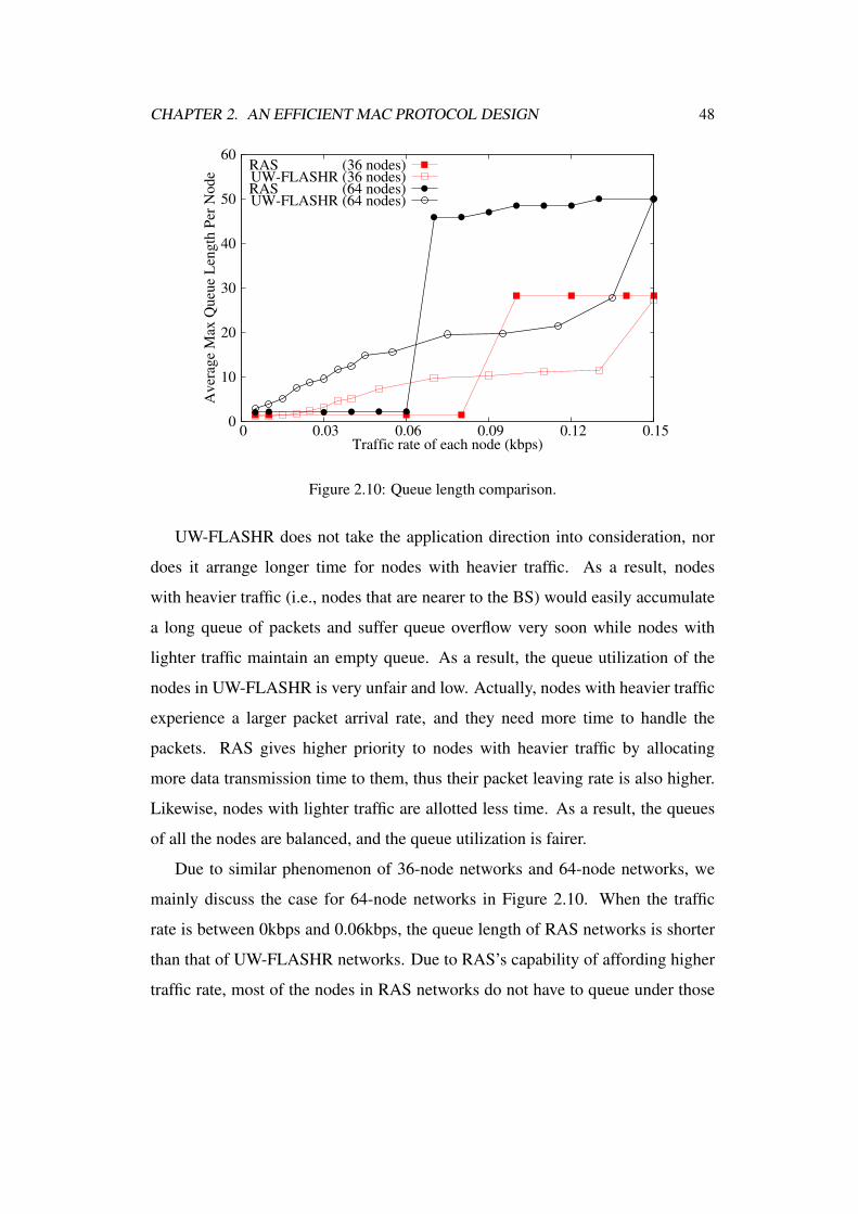
CHAPTER 2. AN EFFICIENT MAC PROTOCOL DESIGN 48
0
10
20
30
40
50
60
0 0.03 0.06 0.09 0.12 0.15
Av
erag
e M
ax Q
ueu
e L
eng
th P
er N
od
e
Traffic rate of each node (kbps)
RAS (36 nodes)UW-FLASHR (36 nodes)RAS (64 nodes)UW-FLASHR (64 nodes)
Figure 2.10: Queue length comparison.
UW-FLASHR does not take the application direction into consideration, nor
does it arrange longer time for nodes with heavier traffic. As a result, nodes
with heavier traffic (i.e., nodes that are nearer to the BS) would easily accumulate
a long queue of packets and suffer queue overflow very soon while nodes with
lighter traffic maintain an empty queue. As a result, the queue utilization of the
nodes in UW-FLASHR is very unfair and low. Actually, nodes with heavier traffic
experience a larger packet arrival rate, and they need more time to handle the
packets. RAS gives higher priority to nodes with heavier traffic by allocating
more data transmission time to them, thus their packet leaving rate is also higher.
Likewise, nodes with lighter traffic are allotted less time. As a result, the queues
of all the nodes are balanced, and the queue utilization is fairer.
Due to similar phenomenon of 36-node networks and 64-node networks, we
mainly discuss the case for 64-node networks in Figure 2.10. When the traffic
rate is between 0kbps and 0.06kbps, the queue length of RAS networks is shorter
than that of UW-FLASHR networks. Due to RAS’s capability of affording higher
traffic rate, most of the nodes in RAS networks do not have to queue under those
CHAPTER 2. AN EFFICIENT MAC PROTOCOL DESIGN 49
traffic rates. Whereas the nodes in UW-FLASHR networks are queueing more and
more packets when traffic gets heavy. In addition, RAS networks undergo a jump
in queue length when the traffic rate increases from 0.06kbps to 0.07kbps. After
this the queue length of RAS networks is much higher than that of UW-FLASHR
networks until they both reach the upper bound 50. This because the queue
utilization of RAS networks is fairer and higher than UW-FLASHR networks. At
traffic rate 0.07kbps, RAS networks start to congest, most of the nodes suffer and
their queues overflow. In contrast, in UW-FLASHR networks, the queues of the
few nodes that are next to the BS are congested at a very low traffic rate while the
queues of faraway nodes are empty. Other nodes get congested gradually with the
increasing traffic rate, thus the queue length does not surge.
Furthermore, because small-scale networks are less likely to suffer congestion,
the queue length of 36-node RAS networks soars at about traffic rate 0.09kbps
rather than at 0.07kbps. It stabilizes at around 27 rather than at 50 when the traffic
rate is larger than 0.11kbps. Eventually, it will stabilize at 50 when the traffic rate
is very high. Nevertheless, 0.15kbps is not a very high traffic rate for 36-node
networks, thus only a majority of the nodes are congested while the others sustain
empty queue. Still the queue length of RAS networks is much larger than that of
UW-FLASHR networks when congestion happens in RAS networks, which again
indicates that the queue utilization of RAS networks is fairer and higher.
In summary, greater maximum queue length allows fairer and higher utilization
of the queue. Correspondingly, the delay upper bound of the RAS networks is
higher than the UW-FLASHR networks because more faraway packets are capable
of arriving at the BS with no overflow in queue.
2.7 Discussions and Conclusions
In this chapter we propose a novel priority-based scheduling algorithm to mitigate
the communication bottleneck of UWASNs. The different characteristics of

CHAPTER 2. AN EFFICIENT MAC PROTOCOL DESIGN 50
communication and node scheduling between UWASNs and traditional TWSNs
are investigated. We then formulate the scheduling problem for UWASNs and
analyze its complexity. We provide a heuristic algorithm to solve the scheduling
problem with a newly designed scheduling-based MAC protocol, called RAS.
RAS gives higher priority to nodes with heavier loads. We compare RAS with
UW-FlASHR. The simulation results demonstrate that RAS not only effectively
improves the throughput and delay, but also increases the queue utilization and
fairness. Compared with the distributed methods, RAS requires synchronization
among sensor nodes. Since the synchronization accuracy in UWASNs is not
required as high as that in TWSNs, the synchronization cost is worthy of the
throughput and delay performance improvement.
2 End of chapter.
Chapter 3
A Reliable MAC Protocol Design
Underwater acoustic sensor networks (UWASNs) are playing a key role in ocean
applications. Unfortunately, besides the inefficiency, UWASNs also suffer from
the unreliability caused by packet loss. Many MAC protocols are proposed to
improve the efficiency of UWASNs, but few of them consider the reliability
of UWASNs even though the packet loss can fail the applications. Actually, a
few of the protocols employ the traditional acknowledgement (ACK) mechanism,
but they suffer the throughput degradation a lot. In this chapter, based on the
efficient MAC protocol RAS proposed in the previous chapter, we design a reliable
RAS called RRAS that obtains a tradeoff between reliability and efficiency.
RRAS designs an ACK and retransmission mechanism that is different from the
traditional one, so that it can maintain a comparable throughput when improving
the reliability. On one hand, the ACK and retransmission do not follow the
data loss immediately. On the other hand, though distributed, the retransmission
mechanism is based on ALOHA, a technique seldom used in wireless networks.
Extensive evaluations are conducted to verify that RRAS achieves a tradeoff on
reliability and efficiency.
51
CHAPTER 3. A RELIABLE MAC PROTOCOL DESIGN 52
3.1 Introduction
A UWASN is composed of underwater sensor nodes that engage sound to transmit
information collected in the ocean. The reason to utilize sound is that radio
frequency (RF) signals used by terrestrial wireless sensor networks (TWSNs) can
merely transmit a few meters in the water [40] [44]. Although UWASNs and
TWSNs are similar, there still exist many differences that make UWASNs less
efficient than TWSNs [11] [44] [86] [105]. First, the acoustic sensor is more
expensive than the terrestrial sensor and thus the sensor deployment in the water
more sparse. Second, the sound bandwidth is much narrower than RF bandwidth
(e.g., 10 kbps VS. 10 Mbps). Consequently, we should utilize the bandwidth in
UWASNs more efficiently. Third and most importantly, the propagation delay of
UWASNs is far larger than that of TWSNs. Acoustic signals propagate at about
1500 m/s underwater, while RF signals travel at the speed of light in the air [92]. To
transmit a data packet over 1500 meters, it takes 1 s underwater and 5 µs in the air.
Due to the high propagation delay of acoustic signals, the network performance of
UWASNs cannot be achieved as highly as that of TWSNs.
Many existing methods aim at collision avoidance and improving the efficiency
of UWASNs, but they are not reliable. They usually perform best-effort
transmissions rather than guarantee receptions. The loss of important data can
result in serious damage. For example, if the data that contain an extreme
high temperature are lost, it maybe too late to extinguish the fire in the forest.
APCAP [44] utilizes the maximum propagation delay to avoid collisions and MAC
level pipelining to increase efficiency. To avoid the poor throughput caused by
using maximum propagation delay, Peleato and Stojanovic apply a shorter delay
to avoid collision when the communicating nodes are close to each other [87].
In addition, two ALOHA-based MAC protocols [26] improve the efficiency by
reducing the RTS (request to send) and CTS (clear to send) handshaking and
avoiding collisions with the information from the overheard packets. Although

CHAPTER 3. A RELIABLE MAC PROTOCOL DESIGN 53
all these MAC protocols help improve the efficiency of UWASNs, none of them
consider acknowledgements (ACKs) or retransmissions. Since the packet loss may
fail the applications, it is very important to maintain a certain level of reliability
with ACK and retransmission mechanisms. For example, when oil spills are
detected, such event report packets should arrive at the BS in time so that prompt
actions can be taken to prevent pollution spreading. Since they may be lost due to
the volatile environment, they should definitely be equipped with a retransmission
scheme.
On the other hand, existing methods that include ACK mechanisms are not
as efficient as the previous techniques with no ACK mechanisms. For example,
Slotted FAMA [82], UW-FLASHR [131], and the reservation MAC protocol
proposed in [117] realize the traditional ACK technique, but they focus on collision
avoidance rather than on ACK and the retransmission effects.
Due to the volatile wireless environment in UWASNs, packet loss is very
common [11]. Unlike packet collision that can be reduced or manipulated at a
very large extent, this kind of packet loss is out of human control. As a result, we
should implement ACK mechanism and the corresponding retransmissions so as
to improve the network and application reliability. Considering the innate inferior
performance and low bandwidth of UWASNs, we should also avoid deteriorating
the efficiency too much by enabling ACK and retransmissions.
In this chapter, based on RAS, the efficient MAC protocol proposed in
the previous chapter, we design a reliable RAS called RRAS to achieve a
tradeoff between the reliability and the efficiency. Different from RAS whose
period is composed of working portion and sleeping portion, RRAS divides the
sleeping portion into a NACK-retransmission portion and a sleeping portion. The
NACK-retransmission mechanism of RRAS can improve the network reliability.
Specifically, with the scheduling done by RAS, after the working portion,
each node can immediately discover which packets are lost. Then during the
CHAPTER 3. A RELIABLE MAC PROTOCOL DESIGN 54
NACK-retransmission portion, it can ask its children that lose the packets to
retransmit the packets. Since the retransmission is non-deterministic, RRAS uses
a distributed and ALOHA-based method to transmit packets rather than uses
scheduling.
We summarize our contributions as follows:
• (1) We propose RRAS to improve the network reliability.
• (2) Extensive evaluations are conducted to show that RRAS achieves higher
reliability than RAS while achieving comparable throughput performance.
In the remainder of this chapter, Section 3.2 describes related work. RRAS
protocol is designed in Section 3.3 respectively. The performance is evaluated in
Section 3.4. Finally, Section 3.5 concludes the chapter.
3.2 Related Work
Recently, there are extensive research efforts focusing on improving the
performance of UWASNs, which are surveyed in aspects of ACK mechanisms
and efficiency as follows.
Slotted FAMA [82] is a handshaking-based protocol designed to avoid
collisions caused by the hidden terminal problem in UWASNs. While it can
efficiently avoid collision caused by the long propagation of UWASNs and also
enable ACK mechanism, it does not utilize the long propagation delay to improve
the throughput and delay performance. By utilizing the long propagation delay in
the communications, Our RRAS can improve the reliability and efficiency.
The reservation MAC protocol proposed in [117] avoids collisions and
improves the bandwidth utilization by employing two channels: a control channel
for RTS/CTS handshake and a data channel for data transmission. It increases the
network throughput by dividing a larger group of collision sources into smaller
ones. While it realizes traditional ACK technique, it does not investigate the
CHAPTER 3. A RELIABLE MAC PROTOCOL DESIGN 55
retransmission effects. In addition, it is based on a single-hop topology and the
gateway is in charge of the control packet and data packet coordination. Hence this
MAC protocol does not suit the multi-hop situation, whose complexity requires a
different analysis. In contrast, RRAS can be applied in either one-hop or multi-hop
topologies.
APCAP identifies that the traditional CSMA leads to poor performance in
UWASNs due to the long propagation delay [44]. Therefore, it utilizes the
maximum propagation delay to avoid collisions. To avoid the poor throughput
caused by such method, Peleato and Stojanovic reduce the delay used to
avoid collision [87]. In addition, APCAP employs MAC level pipelining
to increase efficiency. Another MAC protocol UW-FLASHR [131] also
implements MAC level pipelining. The difference is that APCAP is based on
an adaptive and distributed RTS/CTS handshake while UW-FLASHR employs
both TDMA mechanism and RTS/CTS handshaking. APCAP does not consider
acknowledgements (ACKs) for the data packets while UW-FLASHR enables
traditional ACK mechanisms.
In the above discussed techniques, slotted FAMA [82], UW-FLASHR [131],
and the reservation MAC protocol proposed in [117] realize the traditional ACK
technique, but they focus on collision avoidance rather than on ACK and the
retransmission effects. Since packet loss is very common in WSNs [11], our RRAS
can greatly improve the network and application reliability.
3.3 RRAS Protocol
Since packet loss is very common in UWASNs [11], RAS is not reliable.
By enlarging the guard time, we can avoid collisions caused by imprecise
synchronization. Hence, in our case, we focus on the packet loss caused by the
volatile wireless environment. Because RAS does not considering the ACK and
retransmission problem, we propose a reliable RAS called RRAS. RRAS employs
CHAPTER 3. A RELIABLE MAC PROTOCOL DESIGN 56
Whole Period: Tc
Ts
Td Tg
Time Slot 1 Time Slot Time Slot
Ts
Retransmission
Period
DATA transmission Period: Tw
Sleeping Period
Tr
Figure 3.1: RRAS cycle.
the RAS scheduling to transmit all the DATA efficiently. For the DATA packets
lost during the scheduling, RRAS utilizes the NACK-retransmission mechanism
to improve the overall system reliability.
3.3.1 Overview of NACK-retransmission Mechanism
In the scheduling of RAS, each node n knows nc, the number of packets that should
be received from each of its child node c, and n0, the number of packets generated
by itself. The total packets that should be sent to its parent are n0 +∑
c nc. In
RRAS protocol, if in a cycle, a node does not receive the expected packets, it
would keep the packet loss in mind and perform retransmission in the following
retransmission period.
Retransmission period is part of a RRAS cycle as shown in Figure3.1. RRAS
cycle is designed from RAS cycle: the DATA transmission period of RAS is
kept while the sleeping period of RAS is divided into the retransmission period
and a shorter sleeping period. In this way, the DATA lost in data transmission
period Tw can be retransmitted in retransmission period Tr. Obviously, RRAS
protocol keeps the nodes working for a longer period than RAS for the sake of
reliable transmission. However, since the unavoidable packet loss might fail the
applications, it is worthy of the extra time Tr to keep all the nodes waiting for
possible DATA retransmission requirement.
The packet loss caused by the volatile wireless environment is random, thus
we do not know which packets will be lost in the data transmission period Tw,
CHAPTER 3. A RELIABLE MAC PROTOCOL DESIGN 57
and we cannot schedule the retransmission as we schedule the periodical DATA
transmission. As a result, we employ a NACK-retransmission mechanism, i.e.,
the NACK packet asks for the lost packets, and the retransmission packets reply
NACK with the required packets. The detailed explanation follows.
During retransmission period Tr, the node n that has not received the expected
packets would send a control packet (NACK) to its child node c whose packets
to n are lost during transmission. The NACK contains the packet sequence
numbers that n has received from c. On receiving the NACK, c would know
which packets to retransmit. If node n failed to receive packets from multiple
child nodes, it would send a NACK to the very child nodes one by one. If the
retransmissions succeed, no more retry is needed. Otherwise, node n could initiate
the corresponding retransmission by sending another NACK.
3.3.2 Retransmission Mechanism
The more times that node n retries the transmissions, the higher the reliability
is. Although such retransmission is aimed at improving the DATA transmission
reliability, it does not promise 100% success which would cost a lot of extra
resources. Hence, in our case, we only focus on one-time retry rather on the
frequently used three-time retry [133]. If we want to retry a second time, we
can simply add another retransmission period to retransmit the DATA packets lost
during the first retransmission period.
After receiving NACK, node c would retransmit the lost DATA packets in a
batch or in a burst to node n. Since the control frame exchanges deteriorate the
UWASN efficiency greatly, batch DATA transmission improves the retransmission
throughput and delay performance by reducing the exchanges.
As for the collision avoidance, in order not to degrade the efficiency, we do not
use the maximum propagation delay to avoid collisions as [44] and [82] do. In
addition, carrier sense and RTS/CTS handshaking are efficient in a network where
CHAPTER 3. A RELIABLE MAC PROTOCOL DESIGN 58
the propagation delay is negligible, but they are inefficient in UWASNs [43]. As
a result, we adopt a simple ALOHA mechanism [9] [26]. According to [127],
the propagation time is usually larger than the data duration time (100ms) as long
as the distance between the nodes is larger than 150m. In this situation, even if
the two nodes send packets to each other simultaneously, no collision happens.
Furthermore, if node A and node B start to send a packet to C at the same time, as
long as the difference between A-C distance and B-C distance is larger than 150m,
there will be no collision at node C. For these reasons, we employ simple ALOHA,
i.e., a node could transmit a packet when it is not receiving or transmitting.
Although this mechanism does not guarantee collision-free situations, it is more
efficient. In case collision happens, further actions can be taken: retransmit the
collided packets again or ignore it and accept the current reliability level. In our
work, we study the effects of ALOHA through experiments and prove its influence
on the efficiency and reliability.
We define the states of a node after the DATA transmission period as (α, β).
The α state is determined by the node itself while the β state is determined by its
parents.
α =
Y, packets from its child nodes are lost
N, packets from its child nodes are not lost
β =
Y, packets to its parent nodes are lost
N, packets to its parent nodes are not lost
A node might be in 4 situations: (N,N), (N,Y), (Y,N), (Y,Y). If it it in state
(N,N) with no packet loss, it is free from sending or receiving packets. If it is in
state (N,Y), it does not know that its DATA transmissions to its parents are lost
until it receives the NACKs from its parents. In this case, it will only retransmit
the DATA packets designated in the NACKs.

CHAPTER 3. A RELIABLE MAC PROTOCOL DESIGN 59
If it is in state (Y,N), it knows that DATA transmissions from its child nodes
are lost. It is also aware that since it fails to forward the lost packets to its parent
nodes, its parent nodes will require them through NACK. It should first ask its
child nodes for the lost packets by sending NACKs to them. Next, after collecting
the lost packets from its child nodes, it should forward them to its parent nodes.
Since it does not know the beta state, it does not know whether its parent nodes
will ask for lost packets generated by its child nodes or packets generated by itself.
As a result, even if it has finished collecting the lost packets from its child nodes,
it still should wait to retransmit until receiving the NACKs from its parents.
The actions in state (Y,Y) is similar to those in state (Y,N). The only difference
is that the node should send the lost packets from both its child nodes and from
itself to its parent nodes. In summary, the retransmission will be triggered only
after receiving the NACK requirements.
3.3.3 Retransmission Time
In addition, the length of Tr and extra energy consumption E for reliable
transmission is closely related to the packet loss rate R. The overall energy
consumption is dominated by the transmit power Et, as compared to receive power
Er and idle power Ei [16] [39]. If R is low, then E is low. For example, if R is
0, i.e., there is no packet loss during Tw, then no retransmission is needed, and all
the nodes are idling during Tr with low extra power consumption. If the packet
loss rate is very high during Tw, then the retransmission period Tr should be long
enough to finish all retransmissions, and the extra power would be a lot. In other
words, high packet loss means that the wireless environment is very severe, and
retransmission is required no matter what kind of mechanisms are employed for
DATA transmissions.
Given packet loss rate R, to ensure that the time duration is long enough for
retransmitting the lost packets, the length of Tr for a given network topology is

CHAPTER 3. A RELIABLE MAC PROTOCOL DESIGN 60
calculated as follows.
To make sure that Tr can accommodate all retransmission situations, we
analyze the worst case. Consider the nodes in the longest route to the BS, from the
leaf node a to the BS, and the maximum hop distance is H .
If a DATA transmission from node a to its parent b is lost, then all the nodes
in the route need to retransmit the lost DATA to the BS. A node will retransmit
only on receiving the NACK requirement, then a retransmission between a pair of
nodes would take at most 2 ∗ (Tp + Ts), in which Tp is the maximum propagation
delay and Ts is the time slot. The longest time taken for retransmitting the DATA
to the BS is consequently
2 ∗H ∗ (Tp + Ts). (3.1)
The ALOHA retransmission mechanism only restricts the order between the
NACK and its corresponding retransmission, i.e., it allows parallel transmission
among NACKs from different nodes. As a result, the time used is much less, i.e.
(Tp + Ts) +H ∗ (Tp + Ts). (3.2)
The first term (Tp+Ts) is used to transmit the NACKs, the second term H∗(Tp+Ts)
is used to transmit the lost DATA to the BS.
We then consider the case that more than one packet are lost in such a route.
The worst situation is that all the packets are lost on the way from a to b. The batch
DATA transmission mode reduces the NACK-retransmission handshake, and keeps
the handshake round to be 1 among a node pair. Hence the longest time taken for
retransmitting all the DATA to the BS is
(Tp + Ts) +H ∗ (Tp + Lp ∗ Ts), (3.3)
in which Lp is the total number of DATA packets lost.
Lp = Ap ∗R, (3.4)
given Ap, the number of all the packets to be transmitted in a cycle.
CHAPTER 3. A RELIABLE MAC PROTOCOL DESIGN 61
Next consider the case that more than one route, ro routes, experience DATA
loss. The worst situation is that all the routes are H hops from the BS, and there
is no overlap between any of the routes until they converge at the BS. In this
situation, the batch DATA transmission mechanism cannot be applied to reduce
the time. Then we get the length of Tr that is long enough for most retransmission
situations as:
Tr = ro ∗ (Tp + Ts) + ro ∗H ∗ (Tp + Lp ∗ Ts), (3.5)
When the rough distances between nodes and the routing are known, H and
maximum ro are determined, then Tr can be calculated. However, this value
is too large for a real deployment and hence wastes retransmission time. In
fact, not all DATA losses happen on the way from the farthest nodes to their
parents. In addition, the interference between the routes may be very light, and
the transmissions in each route can happen simultaneously without affecting each
other. Furthermore, the propagation time to transmit 1 DATA packet for 1 hop is
less than the maximum propagation delay Tp. As a result, the actual retransmission
time needed is far less than that indicated in Equation 3.5, and it should be adjusted
accordingly. As our later experiments prove, simulation can help us select a better
value for Tr.
3.4 Performance Evaluation
The protocol performance is simulated using the parameters shown in Table 2.1.
We use the ns-3 setdest tool to generate networks with size ranging from 9 nodes to
64 nodes [3]. For example, the 64-node network covers a 5 km by 5km area, and it
is connected without holes. The maximum one-way propagation time is 1000 ms
calculated from the 1500m transmission range and sound speed. The efficiency
and reliability performance of RRAS is compared to RAS and the traditional
CSMA/CA used in TWSNs.
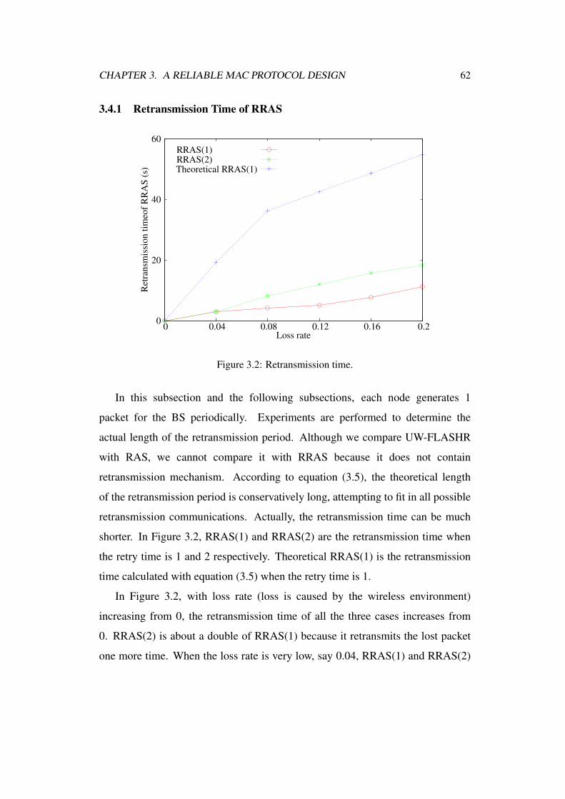
CHAPTER 3. A RELIABLE MAC PROTOCOL DESIGN 62
3.4.1 Retransmission Time of RRAS
0
20
40
60
0 0.04 0.08 0.12 0.16 0.2
Retr
an
smis
sio
n t
imeo
f R
RA
S (
s)
Loss rate
RRAS(1) RRAS(2) Theoretical RRAS(1)
Figure 3.2: Retransmission time.
In this subsection and the following subsections, each node generates 1
packet for the BS periodically. Experiments are performed to determine the
actual length of the retransmission period. Although we compare UW-FLASHR
with RAS, we cannot compare it with RRAS because it does not contain
retransmission mechanism. According to equation (3.5), the theoretical length
of the retransmission period is conservatively long, attempting to fit in all possible
retransmission communications. Actually, the retransmission time can be much
shorter. In Figure 3.2, RRAS(1) and RRAS(2) are the retransmission time when
the retry time is 1 and 2 respectively. Theoretical RRAS(1) is the retransmission
time calculated with equation (3.5) when the retry time is 1.
In Figure 3.2, with loss rate (loss is caused by the wireless environment)
increasing from 0, the retransmission time of all the three cases increases from
0. RRAS(2) is about a double of RRAS(1) because it retransmits the lost packet
one more time. When the loss rate is very low, say 0.04, RRAS(1) and RRAS(2)
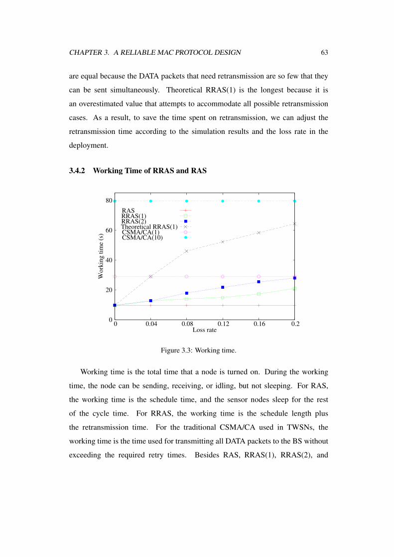
CHAPTER 3. A RELIABLE MAC PROTOCOL DESIGN 63
are equal because the DATA packets that need retransmission are so few that they
can be sent simultaneously. Theoretical RRAS(1) is the longest because it is
an overestimated value that attempts to accommodate all possible retransmission
cases. As a result, to save the time spent on retransmission, we can adjust the
retransmission time according to the simulation results and the loss rate in the
deployment.
3.4.2 Working Time of RRAS and RAS
0
20
40
60
80
0 0.04 0.08 0.12 0.16 0.2
Wo
rkin
g t
ime
(s)
Loss rate
RAS RRAS(1) RRAS(2) Theoretical RRAS(1)CSMA/CA(1) CSMA/CA(10)
Figure 3.3: Working time.
Working time is the total time that a node is turned on. During the working
time, the node can be sending, receiving, or idling, but not sleeping. For RAS,
the working time is the schedule time, and the sensor nodes sleep for the rest
of the cycle time. For RRAS, the working time is the schedule length plus
the retransmission time. For the traditional CSMA/CA used in TWSNs, the
working time is the time used for transmitting all DATA packets to the BS without
exceeding the required retry times. Besides RAS, RRAS(1), RRAS(2), and
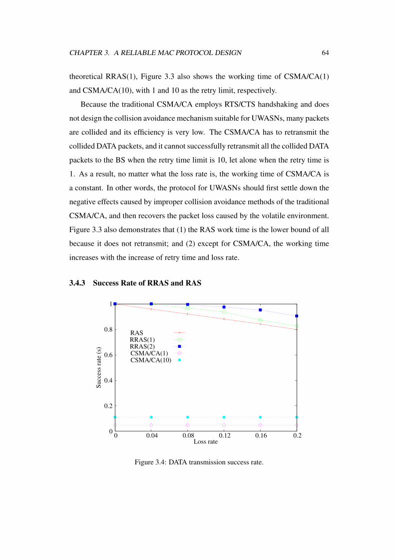
CHAPTER 3. A RELIABLE MAC PROTOCOL DESIGN 64
theoretical RRAS(1), Figure 3.3 also shows the working time of CSMA/CA(1)
and CSMA/CA(10), with 1 and 10 as the retry limit, respectively.
Because the traditional CSMA/CA employs RTS/CTS handshaking and does
not design the collision avoidance mechanism suitable for UWASNs, many packets
are collided and its efficiency is very low. The CSMA/CA has to retransmit the
collided DATA packets, and it cannot successfully retransmit all the collided DATA
packets to the BS when the retry time limit is 10, let alone when the retry time is
1. As a result, no matter what the loss rate is, the working time of CSMA/CA is
a constant. In other words, the protocol for UWASNs should first settle down the
negative effects caused by improper collision avoidance methods of the traditional
CSMA/CA, and then recovers the packet loss caused by the volatile environment.
Figure 3.3 also demonstrates that (1) the RAS work time is the lower bound of all
because it does not retransmit; and (2) except for CSMA/CA, the working time
increases with the increase of retry time and loss rate.
3.4.3 Success Rate of RRAS and RAS
0
0.2
0.4
0.6
0.8
1
0 0.04 0.08 0.12 0.16 0.2
Su
ccess
rate
(s)
Loss rate
RAS RRAS(1) RRAS(2) CSMA/CA(1) CSMA/CA(10)
Figure 3.4: DATA transmission success rate.
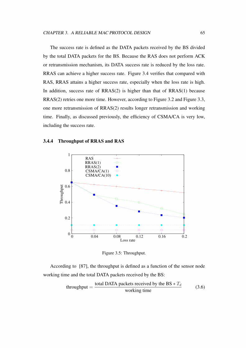
CHAPTER 3. A RELIABLE MAC PROTOCOL DESIGN 65
The success rate is defined as the DATA packets received by the BS divided
by the total DATA packets for the BS. Because the RAS does not perform ACK
or retransmission mechanism, its DATA success rate is reduced by the loss rate.
RRAS can achieve a higher success rate. Figure 3.4 verifies that compared with
RAS, RRAS attains a higher success rate, especially when the loss rate is high.
In addition, success rate of RRAS(2) is higher than that of RRAS(1) because
RRAS(2) retries one more time. However, according to Figure 3.2 and Figure 3.3,
one more retransmission of RRAS(2) results longer retransmission and working
time. Finally, as discussed previously, the efficiency of CSMA/CA is very low,
including the success rate.
3.4.4 Throughput of RRAS and RAS
0
0.2
0.4
0.6
0.8
1
0 0.04 0.08 0.12 0.16 0.2
Th
rou
gh
pu
t
Loss rate
RAS RRAS(1) RRAS(2) CSMA/CA(1) CSMA/CA(10)
Figure 3.5: Throughput.
According to [87], the throughput is defined as a function of the sensor node
working time and the total DATA packets received by the BS:
throughput =total DATA packets received by the BS ∗ Td
working time(3.6)

CHAPTER 3. A RELIABLE MAC PROTOCOL DESIGN 66
In consistency with the poor success rate, the traditional CSMA/CA efficiency
is also very low in Figure 3.5. As discussed in subsection retransmission time,
the throughput of the traditional CSMA/CA is determined by its poor collision
avoidance method rather than by the packet loss rate caused by the environment,
hence it is flat. According to Figure 3.5, the throughput of RAS is the highest, but
the throughput performance of RRAS is not greatly reduced, especially when the
loss rate is not very high. Since the success rate of RRAS is much higher than
RAS according to Figure 3.4, we can observe that RRAS obtains a good tradeoff
between the reliability and the throughput.
3.5 Conclusions
In this chapter, we propose RRAS, a reliable RAS, to achieve a tradeoff between
the reliability and efficiency performance in UWASNs. To improve the throughput,
RRAS employs the efficient RAS scheduling to transmit the majority of the
DATA generated in a cycle to the BS. Then it designs a NACK-retransmission
mechanism to retransmit the DATA packets lost during the previous DATA
transmissions. Because this new NACK-retransmission mechanism is based on the
RAS scheduling that allows each node to know the packets it should receive during
a cycle, it can trigger the NACK requirement after a node identifies its lost packets.
Both the NACK and retransmission packet transmissions are distributed. They are
based on ALOHA so as to reduce the control frame handshaking and improve
throughput. The simulation results demonstrate that RRAS not only effectively
improves the reliability through retransmission, but also attains a comparable
throughput.
2 End of chapter.
Chapter 4
Reliable Protocol Conformance
Testing
Despite the various applications of WSNs, experiences from real WSN
deployments show that protocol implementations in sensor nodes are susceptible
to software failures, which may cause network failures or even breakdown. To
ensure reliable communications for WSNs, pre-deployment protocol conformance
testing is essential. Unfortunately, existing solutions with simulators cannot test
the exact hardware and implementation environment as real sensor nodes, whereas
testbeds are expensive and limited to small-scale networks and topologies.
In this chapter, we present RealProct, a novel and reliable framework for
testing protocol implementations against their specifications in WSNs. RealProct
utilizes real sensor nodes for protocol conformance testing to ensure that the
results are close to the real deployment. Using different techniques from those
in simulations and real deployments, RealProct virtualizes a large network with
any topology and generate non-deterministic events using only a small number of
sensor nodes to provide flexibility and to reduce cost. The framework is carefully
designed to support efficient testing in resource-limited sensor nodes. Moreover,
test execution and verdict are optimized to minimize the number of runs, while
67

CHAPTER 4. RELIABLE PROTOCOL CONFORMANCE TESTING 68
guaranteeing satisfactory false positive and false negative rates. We implement
RealProct and test it with the µIP TCP/IP protocol stack and a routing protocol
developed for WSNs in Contiki-2.4. The results demonstrate the effectiveness of
RealProct by detecting several new bugs and all previously discovered bugs in
various versions of the µIP TCP/IP protocol stack.
4.1 Introduction
Protocols play an important role in WSNs for reliable communication and
coordination [13] [15]. However, experiences from real deployments show that
protocol implementations in sensor nodes are susceptible to software failures
despite pre-deployment testing [15] [50] [66] [135]. Even though specifications
are available for standardized protocols, it is still very hard to assure flawless
protocol implementations by software developers. Misinterpretation of the
specification or software bugs in implementation could both cause communication
failures [13] [135], and even breakdown of the whole network. The bugs can
be very expensive and difficult to fix after deployment [72] [102]. Although
simulations are applied to detect software bugs for WSNs before deployment
[72] [102], it is widely believed that simulations may miss bugs that are
only exposed in real hardware and execution environment. Although testbeds
are considered for pre-deployment testing, they are expensive and limited to
small-scale networks. In addition, most of the existing testbeds are designed
for network performance evaluation rather than software bug detection [75]. To
uncover as many problems as possible, the best method is to test with large-scale
real WSNs which are, however, too expensive.
To settle the above problem and achieve an effective tradeoff between
large-scale real deployment and simulation, we present RealProct (reliable
Protocol conformance testing with Real sensor nodes) that uses a few low-cost
real sensor nodes to mimic large-scale real WSNs and then perform protocol

CHAPTER 4. RELIABLE PROTOCOL CONFORMANCE TESTING 69
conformance testing for WSNs reliably and cost-effectively. With RealProct, the
testing is the closest to the real deployment while the cost is kept at a low level.
RealProct is motivated by protocol conformance testing (PCT), an authoritative
method to check the consistency between a protocol implementation and its
specification [5]. To test a protocol with RealProct, the tester only needs to design
a set of abstract test cases according to the protocol specification [18]. Although
PCT have been applied for Internet, 3G network, WiMAX network [8] [14], its
applications for WSNs have not yet been investigated.
We observe that WSNs that are dramatically different from the traditional
networks. Moreover, RealProct is also very distinct from the simulations and
real deployments. As a result, several major research challenges exist. First,
sensor nodes are resource-constrained devices, so they are unable to provide the
same facilities and operations as the standardized PCT test system. For example,
the sensor node is incapable of storing all the test cases in its limited memory.
Second, a sensor node in the PCT test system is more difficult to be controlled
than a personal computer (PC). A sensor node usually does not provide proper
user interface, so operation commands are sent to the node mainly relying on the
serial ports connecting to the computer. Third, the volatile wireless environment
in WSNs will result in random packet loss [15]. The loss may trigger the potential
protocol bugs and results in instability and unreliability in our tests, such as false
positive and false negative errors [83]. Finally, RealProct only employs a few real
sensor nodes, and hence it seems that it is unable to test the protocol with various
topologies and events as the simulations and high-cost real deployments.
To attack the challenges, our major contributions are as follows:
• We propose RealProct as a generic and cost-effective architecture for
protocol conformance testing in WSNs that makes use of only two real sensor
nodes and a personal computer (PC). The PC helps storing all the test cases
which will be handed over to the sensor nodes in real time. The framework

CHAPTER 4. RELIABLE PROTOCOL CONFORMANCE TESTING 70
enforces abstracting the protocol interfaces to build up a library for concise
control of the sensor nodes through serial ports.
• Three different techniques (not utilized in simulations and real deployments)
are proposed to make RealProct practical and reliable for WSN protocol
conformance testing: topology virtualization, event virtualization, and
dynamic test execution. The topology virtualization technique imitates
WSNs with different structures using a few sensor nodes, while the event
virtualization generates non-deterministic events. Dynamic test execution
can tackle the inaccuracy problem caused by non-deterministic events when
generating the test verdict.
• We provide case studies with real experiments to prove the feasibility of
RealProct. RealProct effectively discovers two new bugs verified by the
developers, and identifies all the previously detected bugs in the µTCP/IP
stack [32] [34] [35] of Contiki-2.4 [33]. It also validates the Rime mesh
routing protocol in Contiki-2.4. The source code for finding the bugs is
available online1.
The remainder of this chapter is organized as follows. Section 4.2 discusses
the related work. Section 4.3 presents the background of PCT. We design the
framework of RealProct for protocol conformance testing in WSNs in Section
4.4, and propose three novel techniques to make RealProct practical for WSNs
in Section 4.5. After discussing the generality of RealProct in Section 4.6, we
evaluate its feasibility with two case studies in Section 4.7. Finally, Section 4.8
concludes the chapter.1http://www.cse.cuhk.edu.hk/˜jjxiong/testcases/testcase.htm

CHAPTER 4. RELIABLE PROTOCOL CONFORMANCE TESTING 71
4.2 Related Work
It is necessary to extensively test and debug WSN protocols before real
deployment. If the bugs sneak into deployment, they are very difficult to detect
and costly to fix. Currently, the classification between testing and debugging in
WSNs is not very clear. We define testing as the techniques of detecting failures
or abnormal phenomena and debugging as techniques that diagnose the precise
nature of a known error and then correcting it [45]. In other words, helping locate
the errors in program code or root cause of failures is the process of debugging.
Only after testing detects abnormal behaviors will debugging be triggered.
Existing approaches for testing and debugging WSN protocols fall into three
main categories: program analysis tool and simulator (testing before deployment),
real deployment (testing after deployment), and debugger. We consider testing
as the technique for detecting failures or abnormal behaviors, while debugging as
the process for diagnosing the precise nature of a known error [45]. Only after
abnormal behaviors are detected in testing, debugging will be triggered.
Program analysis tools and simulators are very useful in detecting errors
and verifying algorithms of the protocols. Safe TinyOS [28] is compile-time
program analysis tool that can avoid memory corruption before program execution.
Neutron’s compiler and runtime extensions [25] help the programs to efficiently
recover from memory safety bugs. FSMGen [63] derives FSM from TinyOS [69]
application so as to help the programmer detect the software errors at a
system level. Well-known simulation tools include ns-3 [3], a general network
simulator, TOSSIM [68], a simulator for TinyOS WSNs, and Avrora [89] [116],
a cycle-accurate instruction-level simulator. Several tools developed for finding
software bugs in WSNs are based on simulation. T-Check [72] is an event-driven
simulator based on TOSSIM and Safe TinyOS. It employs the model checker
in [59]. KleeNet [102] is based on the low-level symbolic virtual machine
KLEE [21]. Given the fact that nodes in a simulation environment and real sensor

CHAPTER 4. RELIABLE PROTOCOL CONFORMANCE TESTING 72
nodes are different, protocol execution in simulations may not be able to discover
all software problems that will occur in real sensor nodes.
Different from simulations, testing during protocol execution in real sensor
nodes is crucial in detecting software bugs. Kothari et al. [64] presents HERMES,
a lightweight framework and prototype tool that provides fine-grained visibility
and control of a sensor node’s software at run-time. HERMES’s architecture is
based on the notion of interposition, which enables it to provide these properties
in a minimally intrusive manner, without requiring any modification to software
applications being observed and controlled. HERMES provides a general,
extensible, and easy-to-use framework for specifying which software components
to observe and control, as well as when and how the observation and control is
done. Sympathy [95] actively collects run-time status from sensor nodes, such as
routing table and flow information, and detects possible faults by analyzing the
information. To save the energy for collecting logs, PassiveDiagnosis [75] and
PassiveAssertions [101] both passively record the logs from real deployment by
piggybacking the logs in regular data packets. NodeMD [65] is a deployment
management system that successfully implements lightweight run-time detection,
logging, and notification of software faults. Although these run-time testing
method can detect real-time failures in real deployment, it is costly and very
difficult to detect and fix errors after deployment. Similarly, testbeds could
be applied for testing in real nodes, but they are expensive and limited to
small-scale networks [75]. Moreover, existing testbeds are often designed for
network performance evaluation rather than protocol conformance testing [75].
Different from the above work, RealProct uses a few real sensor nodes to perform
protocol conformance test, which can detect bugs on real nodes efficiently before
large-scale deployment.
A number of debuggers have been developed for WSNs. Clairvoyant [132]
is a comprehensive source-level debugger that provides standard debugging

CHAPTER 4. RELIABLE PROTOCOL CONFORMANCE TESTING 73
commands including break, step, watch, and so on. Since it can only debug a
sensor node instead of a network, it cannot handle distributed bugs. Although
some debugging techniques can detect abnormal behaviors, they mainly focus
on locating the root cause of the software bugs. Khan et al. present a
diagnostic simulator to locate possible causes of the user-defined undesirable
behavior when it is encountered during simulation [56]. The simulator works by
logging event sequences and states produced in a regular simulation run. It then
uses sequence extraction and frequent pattern analysis techniques to recognize
sequences and states that are possible root causes. However, this simulator can
only diagnose bugs that occur frequently. Thus, they design another tool called
DustMiner for uncovering bugs due to interactive complexity in networked sensing
applications [57]. Such bugs are often not repeatable, making them particularly
hard to find, as the specific sequence of events that invokes the bug may not be
easy to reconstruct. An extensible framework is developed where a front-end
collects runtime data logs of the system being debugged and an off-line back-end
uses frequent discriminative pattern mining to uncover likely causes of failures.
Sentomist [135] and tracepoints [23] are both automated tools for debugging WSN
applications. The former is built based on simulation and is especially effective
for identifying transient bugs. The latter inserts checkpoints in the applications
to allow run-time debugging. Since debuggers are designed for locating the bugs
after the bugs are detected by testing, they only give a very detailed investigation
on a small part of the codes for locating specific bugs. In this work, we focus
on protocol conformance testing rather than debugging, which allows us to detect
general implementation problems for WSN protocols.
4.3 Protocol Conformance Testing
Due to programming bugs or misunderstanding of the standard specifications,
the protocol implementation always differs from the expected, hindering the

CHAPTER 4. RELIABLE PROTOCOL CONFORMANCE TESTING 74
interoperability between systems implemented by different manufacturers [5] [18].
Hence, testing is necessary. Protocol conformance testing (PCT) is an authoritative
way to check the consistency between the any protocol and its implementation [5].
As functional (black-box) testing, PCT aims to gain confidence in correct
implementation of the protocol (any protocol), so as to force successful
communication between peer protocol entities. An example of a protocol
conformance test would be to check if the ‘ping’ command operates correctly. Ping
should send an ICMP echo request to an operational host or router and the host or
router should return an ICMP echo response. The ‘ping’ command should also be
sent to a non-existent or non-operational host or router, and then report back ‘ping:
unknown host [hostname]’. The latter would be a negative conformance test.
PCT is popular and influential not only in traditional wired networks [18], but
also in wireless networks. The protocol stack in wireless network WiMAX is
tested in a PCT environment provided by Agilent [8], so does 3G protocol stack
tested with PCT toolkit designed by company Anritsu [14]. Those products have
to pass the conformance testing before they get GCF (Global Certification Forum)
approval for an introduction into the market. Despite PCT’s wide application, it
has not yet benefited WSNs due to a number of challenges discussed previously.
4.3.1 PCT Process
The PCT process is shown in Fig. 4.1, in which the protocol implementation
to be tested is called Implementation Under Test (IUT). Its first phase is test
generation, in which abstract test cases for the IUT are designed based on the
protocol specification. Each test case can only have one target, i.e., testing a
particular function of the protocol. A collection of test cases can cover many
aspects of the protocol, and they form a test suite. Formal methods, such as FSM
and extended FSM [18], are employed for deriving the abstract test suite.
The second phase, test implementation, transforms the abstract test cases into
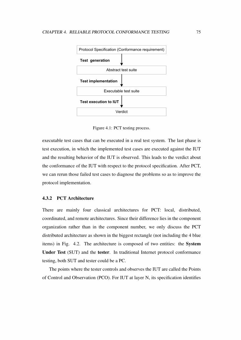
CHAPTER 4. RELIABLE PROTOCOL CONFORMANCE TESTING 75
Abstract test suite
Protocol Specification (Conformance requirement)
Executable test suite
Test execution to IUT
Verdict
Test implementation
Test generation
Figure 4.1: PCT testing process.
executable test cases that can be executed in a real test system. The last phase is
test execution, in which the implemented test cases are executed against the IUT
and the resulting behavior of the IUT is observed. This leads to the verdict about
the conformance of the IUT with respect to the protocol specification. After PCT,
we can rerun those failed test cases to diagnose the problems so as to improve the
protocol implementation.
4.3.2 PCT Architecture
There are mainly four classical architectures for PCT: local, distributed,
coordinated, and remote architectures. Since their difference lies in the component
organization rather than in the component number, we only discuss the PCT
distributed architecture as shown in the biggest rectangle (not including the 4 blue
items) in Fig. 4.2. The architecture is composed of two entities: the System
Under Test (SUT) and the tester. In traditional Internet protocol conformance
testing, both SUT and tester could be a PC.
The points where the tester controls and observes the IUT are called the Points
of Control and Observation (PCO). For IUT at layer N, its specification identifies

CHAPTER 4. RELIABLE PROTOCOL CONFORMANCE TESTING 76
the behavior of a protocol entity at the upper and lower access points (interfaces)
of the protocol. Hence the ideal PCOs to test the IUT are these two access points.
The part that is connected through the upper access point is called the Upper Tester
(UT). Similarly, the part that is connected to the IUT through the lower access point
is called the Lower Tester (LT). The service provider supports the UT, IUT, and LT
implementation.
The tester contains only LT while the SUT contains two logical components:
UT and the IUT. The LT is consisted of executable test cases, and it is a peer entity
of the combination of the UT and the IUT. Each test case execution stimulates
the IUT, and the response of the IUT is observed at PCOs. Test results are
obtained by comparing the observations with the expected behaviors indicated
in the specifications. In other words, the LT provides different kinds of inputs
to IUT, and the outputs of the IUT are compared with the correct behaviors as
specified to arrive at a verdict. When testing IUT, we focus on the operation of
the protocol being tested and consider that the other parts behave correctly. In this
way, the failed test cases can pinpoint the problems in protocol implementation. In
addition, the test coordination helps execute the tests, which includes maintaining
synchronization between the SUT and tester and controlling the execution flow.
4.4 Design of the RealProct Framework
The above PCT design is a general software engineering method for testing
protocol implementation against specifications. However, none of the above four
PCT architectures fit WSNs due to the limited resources of sensor nodes and their
volatile working environment. For this reason, our designed framework for PCT is
different from the previous general one in the 4 blue items as shown in Fig. 4.2. To
unveil as much abnormal behaviors of a protocol implementation in WSNs before
deployment, we utilize two real sensor nodes to work as the tester and the SUT
respectively in a distributed PCT architecture. We explain the unique features of
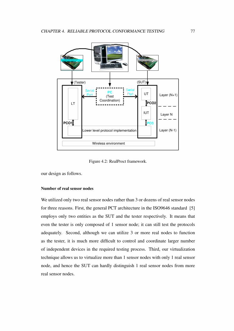
CHAPTER 4. RELIABLE PROTOCOL CONFORMANCE TESTING 77
PC
(Test Coordination)
IUT
LT
UT
Lower level protocol implementation
PCO2
Wireless environment
(Tester) (SUT)
SerialPort
SerialPort
Layer N
Layer (N+1)
Layer (N-1)
PO3PCO1
Figure 4.2: RealProct framework.
our design as follows.
Number of real sensor nodes
We utilized only two real sensor nodes rather than 3 or dozens of real sensor nodes
for three reasons. First, the general PCT architecture in the ISO9646 standard [5]
employs only two entities as the SUT and the tester respectively. It means that
even the tester is only composed of 1 sensor node; it can still test the protocols
adequately. Second, although we can utilize 3 or more real nodes to function
as the tester, it is much more difficult to control and coordinate larger number
of independent devices in the required testing process. Third, our virtualization
technique allows us to virtualize more than 1 sensor nodes with only 1 real sensor
node, and hence the SUT can hardly distinguish 1 real sensor nodes from more
real sensor nodes.
CHAPTER 4. RELIABLE PROTOCOL CONFORMANCE TESTING 78
Coordination
We suggest test coordination to be functioned by a PC, rather than by the tester or
the SUT, due to the limited memory and computation power of the sensor nodes.
Compared with the sensor nodes, PC is a much more powerful device to coordinate
the tests. We connect the PC with the two sensor nodes with serial ports, through
which the PC communicates with the sensor nodes and supply them with power.
Initially, all the test cases are stored in the PC, and each one is downloaded to the
tester for execution one by one.
In addition, the PC maintains test synchronization and controls sequence of
actions between the tester and the SUT. Since we cannot manipulate the system
to be tested (SUT) directly, we control it passively through the tester which will
be installed with all test cases. The details on how we control it will be discussed
in the next section. Furthermore, the PC observes and saves the test execution
logs through the serial ports. These logs are very important for generating the test
verdict and performing bug analysis afterwards. In practice, we do not save the
test execution results in the sensor nodes due to their limited memory. Moreover,
saving logs in the sensor node may alter or even deteriorate the performance of the
IUT. If we store all the logs in the sensor nodes, we will not know the real-time
results of the testing unless the sensor nodes send the logs to the PC. Instead, we
suggest the PC to get real-time results from sensor nodes through the serial port
and save the logs locally.
Resource management
The design of the LT and the UT are modified to better suit the
resource-constrained WSNs. Unlike the traditional PCT framework, the LT and
the UT are simplified for easier control of the tests. The LT is a suite of executable
test cases based on FSM. Each test case in the LT now only targets at one aspect
of the IUT. To make the test case simpler, we apply virtualization techniques to
CHAPTER 4. RELIABLE PROTOCOL CONFORMANCE TESTING 79
imitate a large network by controlling only two nodes rather than managing a large
number of nodes. The UT should be simple, but still be capable to drive the IUT
to send and receive packets. The log generated from the LT and the UT is mainly
about packets in order to relieve the load of the tester and the SUT.
PCO optimization
We further optimize the PCOs for the testing framework and add logging module
for the PCOs. In traditional PCT architectures, one PCO is in the tester and the
other is the SUT. In contrast, our framework adds a point of observation (PO3) in
the SUT as shown in Fig. 4.2. Is it redundant to add such a point? The answer
is no. The traditional distributed PCT architecture assumes that traditionally both
the PCO1 and PO3 observe the same phenomenon. However, this assumption does
not hold due to the volatile wireless environment of WSNs. The LT can control
and stimulate the IUT at PCO1, but it cannot make sure that the packet it sends
will arrive at PO3 without loss, corruption, or duplication. To avoid false positive
(FP) and false negative (FN) errors in test, we double-check the packet content at
PO3.
4.5 RealProct Techniques
RealProct provides a generic framework for testing the implementation of a
wide range of protocols in WSNs. Although it is straightforward to write test
cases based on the specifications, it is difficult for RealProct to fulfill the testing
requirements for different protocols using only limited number of sensor nodes in
practice. To address this limitation, we propose two novel techniques, topology
virtualization and event virtualization, to aid the LT design in order to imitate
WSNs with various topologies and events in our 2-node framework. Apart from
that, testing with real nodes also experiences random packet loss, which might
cause FP and FN errors in test verdict. We thus design a dynamic test execution

CHAPTER 4. RELIABLE PROTOCOL CONFORMANCE TESTING 80
algorithm to reduce the FP and FN error rates down to a required level.
4.5.1 Topology Virtualization
Because the simulations and real deployments are able to verify the protocol
functionality various topologies, they do not need to virtualize topology at
all. However, for RealProct that tests with limited number of nodes, topology
virtualization is necessary to provide higher test case granularity. Unlike
simulation, virtualization in our framework utilizes real hardware. The technique
can virtualize larger scale network with limited real nodes in a way that the SUT
can hardly distinguish them. The idea is that no matter in what kinds of topology,
the SUT can only recognize its environment from the packets it receives. More
importantly, it can only receive packets from the nodes that are placed within its
reception range, i.e., 1-hop neighbor nodes. In practice, the amount of sensor
nodes that are placed within a sensor node’s reception range is limited. Hence,
it is not difficult for the tester to virtualize all the 1-hop neighbors of the SUT.
It seems that the tester can only virtualize 1-hop topologies, but not multi-hop
topologies apparently. However, this is not true. We will show how the packets
from nodes farther away can also be imitated and transmitted to the SUT by
topology virtualization.
Specifically, given two real sensor nodes: the SUT and tester, and the latter can
virtualize for the former a topology composed of node 1, node 2, and node 3 as
shown in the upper portion of Fig. 4.3. The tester sends two routing packets to
the SUT. Since the SUT can receive packet 1 and packet 2 directly, it regards the
nodes that send these packets as its 1-hop neighbors (node 1 and node 2 here). In
addition, packet 2 tells the SUT that it has a neighbor node 3. Since the SUT has
not received any packets from node 3 directly, it adds node 3 as its 2-hop neighbor.
As a result, the SUT experiences as if it has two 1-hop neighbors and one 2-hop
neighbor in a two-level tree topology.

CHAPTER 4. RELIABLE PROTOCOL CONFORMANCE TESTING 81
Addr2
Addr1
Addr3
SUT
Tester
Pac
ket 1
Packet 2
Content of Packet 1:
Sender address is Addr1.
Content of Packet 2:
Sender address is Addr2.
The sender has a
neighbor with Addr3.
Figure 4.3: Topology virtualization demonstration.
In real deployment of this topology, the packet receptions and topology
discovery for the SUT are just the same as those in our virtualized topology.
In other words, as long as the SUT receives the same packets as those in a
real topology, the virtualized topology for the SUT is indistinguishable from the
actual one. With topology virtualization, we can effectively reduce the number of
sensor nodes and the extensive human efforts for protocol conformance testing in
large-scale networks.
Algorithm 4 shows how to virtualize different topologies when testing various
routing protocols. In this case, the routing protocol is IUT, and the real sensor node
installed with IUT is the SUT. The key point to test the SUT in any given topology
is to analyze the effects of different packet transmissions in the SUT, and then to
virtualize the effects for the SUT with the tester.
4.5.2 Event Virtualization
Software bugs are often detected when there are non-deterministic events in
the network, such as node reboot and outage, packet duplication, packet loss,
and so on. These events have potential to drive a WSN application into
corner-case situation, where bugs usually lurk. In order to ensure high coverage

CHAPTER 4. RELIABLE PROTOCOL CONFORMANCE TESTING 82
Algorithm 4 Topology virtualization process for any routing protocol.1: Understand the route discovery mechanism
2: Divide the routing positions in a route into source, forwarder, and destination
3: Divide the nodes into two sets: N1 (SUT’s 1-hop neighbors) and N2 (SUT’s
non-neighboring nodes)
4: while P takes each value in the above three positions do
5: Analyze the effects on the SUT when nodes ∈ N1 send a packet
6: Analyze the effects on the SUT when nodes ∈ N2 send a packet
7: Analyze the responses of nodes ∈ N1 when the SUT sends a packet
8: Analyze the effects of the above responses on the SUT
9: end while
10: Build a model M for effects of packet transmission on the SUT from the previous
analysis
11: Let S be the set of to-be-tested topologies
12: while Based on the model M , ∀Topo ∈ S do
13: Test the SUT when it is communicating with nodes ∈ N1
14: Test the SUT when it is communicating with nodes ∈ N2
15: end while
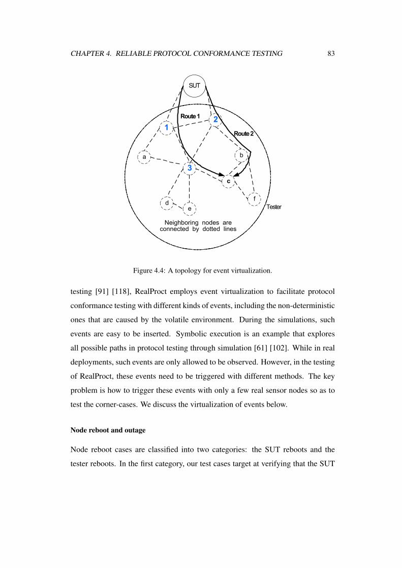
CHAPTER 4. RELIABLE PROTOCOL CONFORMANCE TESTING 83
2
1
b
SUT
f
3
c
d
a
e Tester
Route 1
Route 2
Neighboring nodes are connected by dotted lines
Figure 4.4: A topology for event virtualization.
testing [91] [118], RealProct employs event virtualization to facilitate protocol
conformance testing with different kinds of events, including the non-deterministic
ones that are caused by the volatile environment. During the simulations, such
events are easy to be inserted. Symbolic execution is an example that explores
all possible paths in protocol testing through simulation [61] [102]. While in real
deployments, such events are only allowed to be observed. However, in the testing
of RealProct, these events need to be triggered with different methods. The key
problem is how to trigger these events with only a few real sensor nodes so as to
test the corner-cases. We discuss the virtualization of events below.
Node reboot and outage
Node reboot cases are classified into two categories: the SUT reboots and the
tester reboots. In the first category, our test cases target at verifying that the SUT

CHAPTER 4. RELIABLE PROTOCOL CONFORMANCE TESTING 84
can successfully reboot and return to the initial state. For this case, we just send
to SUT the reboot command ‘/home/user/contiki-2.4/tools/sky/msp430-bsl-linux
–telosb -c /dev/ttyUSB0 -r’ in our experiments. For the second category, the test
cases are checking whether the SUT can appropriately handle the reboot of other
sensor nodes in various topologies. We do not care about which node reboots in
what kind of virtualized topologies. As long as we know the influence of its reboot
in the SUT, we can virtualize node reboot for the SUT by exerting such impacts
on it.
We take the rime mesh routing protocol (RMRP) used in Contiki with the
virtualized topology shown in Fig. 4.4 as an example. The SUT is the only 1-hop
node from the sink, and the application running in the SUT and the tester is sending
data to the sink regularly. The reboot of node 1 has small effects on the SUT.
Before reboot, node 1’s influence on the SUT is its regular data packets and the
related route discovery packets. Hence we virtualize its reboot by not allowing the
tester to send data packets and route discovery packets with source as node 1 to
the SUT. Given that node outage will cause node reboot, the virtualization method
is the same.
Packet disorder, duplication, corruption, and loss
Existing tools, such as KleeNet, have not explored packet disorder in testing. It is
because these tools rely on simulation, model based on human experience [102].
Neither have we realized it until we observed this phenomenon in our testing with
real sensor nodes. We reported this problem to the Contiki developers and believed
that it was caused by the implementations of the lower level protocols and the
volatile wireless channels.
Let us look at the testing of a TCP implementation as an example. Consider the
whole topology in Fig. 4.4, the SUT is the TCP server and node c is the TCP client.
From node c to the SUT, there exist two routes. One is c → b → 2 → SUT, and the
CHAPTER 4. RELIABLE PROTOCOL CONFORMANCE TESTING 85
other is c → 3 → 1 → SUT. If the routing protocol uses two routes simultaneously,
then the packets arrived at the SUT from node c may be disordered. Say, the first
data packet from node c takes route 1 and the second data packet follows route
2. If route 1 is more congested than route 2, the second data packet may arrive at
the SUT before the first data packet, resulting packet disorder at the SUT. If the
SUT cannot handle the disorder appropriately, it fails the test case. To virtualize
the packet disorder with only one tester, it prepares two packets: packet 1 with
a smaller sequence number and packet 2 with a larger sequence number. Then it
sends packet 2 to the SUT first, and packet 1 next.
Packet duplication can be virtualized by sending the same packets to the SUT
twice or multiple times with different intervals. Similarly, packet corruption is
virtualized by distorting different fields of the packet before sending the packet to
the SUT. In order to virtualize the packet loss, the tester will not send the expected
packet or acknowledgment to the SUT.
4.5.3 Dynamic Test Execution
In simulations, we can control when and where the non-deterministic events occur.
However, testing with real sensor nodes is not entirely under human control, and
hence we cannot avoid their occurrences in the cases that we do not anticipate.
Here we focus on unexpected packet loss caused by the volatile environment,
which is the main problem that obstructs our normal testing with real sensor nodes.
The loss may occur to any packets we send or receive during our testing, and hence
threaten our testing and could result in false positive (FP) and false negative (FN)
errors in the test verdict.
PO3 is thus deployed to monitor the difference of packets exchanged between
PCO1 and PO3 during execution (see Fig. 4.2). It can assist human in debugging
problems caused especially by packet loss. Actually, the most convenient way to
avoid FP and FN errors is to repeat the test cases several times so as to filter out the

CHAPTER 4. RELIABLE PROTOCOL CONFORMANCE TESTING 86
volatile influence from the environment. Intuitively, the more times we repeat, the
less likely that FP and FN errors will occur. However, it is inefficient to execute
the test cases for too many times. Thus, here is the problem: What is the minimal
number of executions that can guarantee the FP and FN error rates lower than a
certain level? We design an algorithm to tackle this problem.
Let the empirical probability of packet loss caused by the environment be L0.
Due to packet loss, the test results will be distorted with chance L0, and lead to FP
and FN errors. Suppose a test case is executed n times, and it passes n1 times and
fails n2 times. If n1 > n2, we would like to declare the test as pass (Assertion 1).
If n2 > n1, we would like to declare the test as failure (Assertion 2). If n1 = n0,
we execute the test case for more times until n1 = n0 does not hold. However,
Assertion 1 may suffer FN error if the test verdict should be fail, but was wrongly
concluded as pass. Assertion 2 may suffer FP error if the test verdict should be
pass, but was wrongly concluded as fail. What is the minimum value of n that
guarantees both Assertion 1 suffers FN error and Assertion 2 suffers FP error at a
rate lower than a threshold E, say 1%?
For a test case with n1 > n2, if FN error occurs, then n1 passes are caused
by packet loss and n2 failures are not affected by packet loss. Hence the FN
probability P (FN) is (nn1
)Ln10 (1− L0)
n2 .
Let P (FN) ≤ E, then the smallest n exists if n1 = n, i.e., all the executions
pass. Hence we have the minimum n as
n = ⌈lgEL0⌉.
Similarly, for a test case with n2 > n1, if FP error occurs, then n2 failures are
caused by packet loss and n1 passes are not affected by packet loss. Hence ,the FP
probability P (FP ) is (nn2)Ln2
0
(1− L0)
n1 .

CHAPTER 4. RELIABLE PROTOCOL CONFORMANCE TESTING 87
Algorithm 5 Dynamic test execution process for each test case.
1: Calculate nmin = ⌈lgEL0⌉, n = n1 = n2 = 0
2: while n ≤ nmin do
3: Execute the test case
4: if Execution result is pass then
5: n1++
6: else
7: n2++
8: end if
9: end while
10: loop
11: if n1 > n2. then
12: Calculate P (FN) =(nn1
)Ln10 (1− L0)
n2
13: if P (FN) ≤ E then
14: break //end test execution
15: else
16: Execute the test case and increase n1 or n2 according to the result
17: end if
18: else if n1 < n2. then
19: Calculate P (FP ) =(nn1)Ln2
0
(1− L0)
n1
20: if P (FP ) ≤ E then
21: break //end test execution
22: else
23: Execute the test case and increase n1 or n2 according to the result
24: end if
25: else if n1 = n2 then
26: Execute the test case and increase n1 or n2 according to the result
27: end if
28: end loop

CHAPTER 4. RELIABLE PROTOCOL CONFORMANCE TESTING 88
Similarly, let P (FP ) ≤ E, then the smallest n exists if n2 = n, i.e., all the
executions fails. We also have the minimum n as
n = ⌈lgEL0⌉.
For example, if E = 0.01, L0 = 0.2, then n = 3. That is if we get 3 continuous
passes for a test case, then the chance of FN to declare it as pass is less than 1%.
Therefore, for this case, we can end test case repetition after 3 times. However,
if we get 2 passes and 1 failure, through calculation, P (FN) of declaring pass is
9.6% in this case. Therefore, we have to execute the test case for extra times until
we get P (FN) ≤ E and then declare it as pass, or until we get that n2 > n1 and
P (FP ) ≤ E.
In general, for each test case, it is first executed for ⌈lgEL0⌉ times. If the result is
n1 > n2, then we calculate P (FN) and compare it with E. If P (FN) ≤ E, then
we end the test execution and declare the test case as pass. If the result is n2 > n1,
then we calculate P (FP ) and compare it with E. If P (FP ) ≤ E, we end the
test execution and declare the test case as failure. Otherwise, we repeat the test
case execution until n1 > n2 and P (FN) ≤ E or until n2 > n1 and P (FP ) ≤
E. In this way, the execution repetition of each test case can be minimized in
real-time dynamically according to the requirement of the FN and FP error rates.
The execution process is shown in Algorithm 5.
4.6 Generality of RealProct
RealProct presents a generic framework for testing a wide range of protocols
in WSNs by using only two real sensor nodes and a PC. Three techniques are
designed to make the framework practical for WSNs. Topology virtualization
allows us to test different protocols in various network topologies. Event
virtualization facilitates protocol conformance testing in networks with different
kinds of events, including the non-deterministic ones that are caused by the volatile
CHAPTER 4. RELIABLE PROTOCOL CONFORMANCE TESTING 89
environment, such as node reboot, node outage, packet loss, and packet corruption.
The dynamic test execution and verdict algorithm is used to guarantee the negative
influence caused by the environmental packet loss is lower than a required level.
These techniques and related algorithms are computed in the PC to relieve the
burden of resource-limited sensor nodes.
Although testing diverse protocols in WSNs requires different manual
efforts [5] [118], RealProct provides a generic framework and universal techniques
to keep the testing process the same and easy to follow. A user only needs to
design abstract test cases according to the protocol specification, and then abstract
the interfaces of the protocol implementation and translate those abstract test cases
into executable ones with the aid of our virtualization techniques. The executable
test cases will be stored in the PC. The PC downloads each test case into the tester
node in real-time and trigger the test case execution one by one. Our test execution
and verdict algorithm can control the execution times of each test case and verdicts
the test results autonomously. Finally, the PC can summarize and repeat those
failed test cases to help debugging the problems. The testing methodology is
general rather than designed for a specific protocol.
4.7 Evaluation
This section evaluates the practicability and efficiency of our RealProct for
protocol conformance testing with two case studies. We test the TCP protocol
of the µIP TCP/IP stack for WSNs in Contiki-2.4 because TCP is not only viable
for WSNs, but also very useful to connect WSNs with traditional networks [34].
During the TCP testing, RealProct finds not only two new bugs acknowledged by
the developers, but also all the previously discovered bugs [102]. The Rime mesh
routing protocol (RMRP) designed for WSNs in Contiki-2.4 is also tested. The
test cases for detecting those bugs are available online1. Figure 4.5 shows that the1http://www.cse.cuhk.edu.hk/˜jjxiong/testcases/testcase.htm
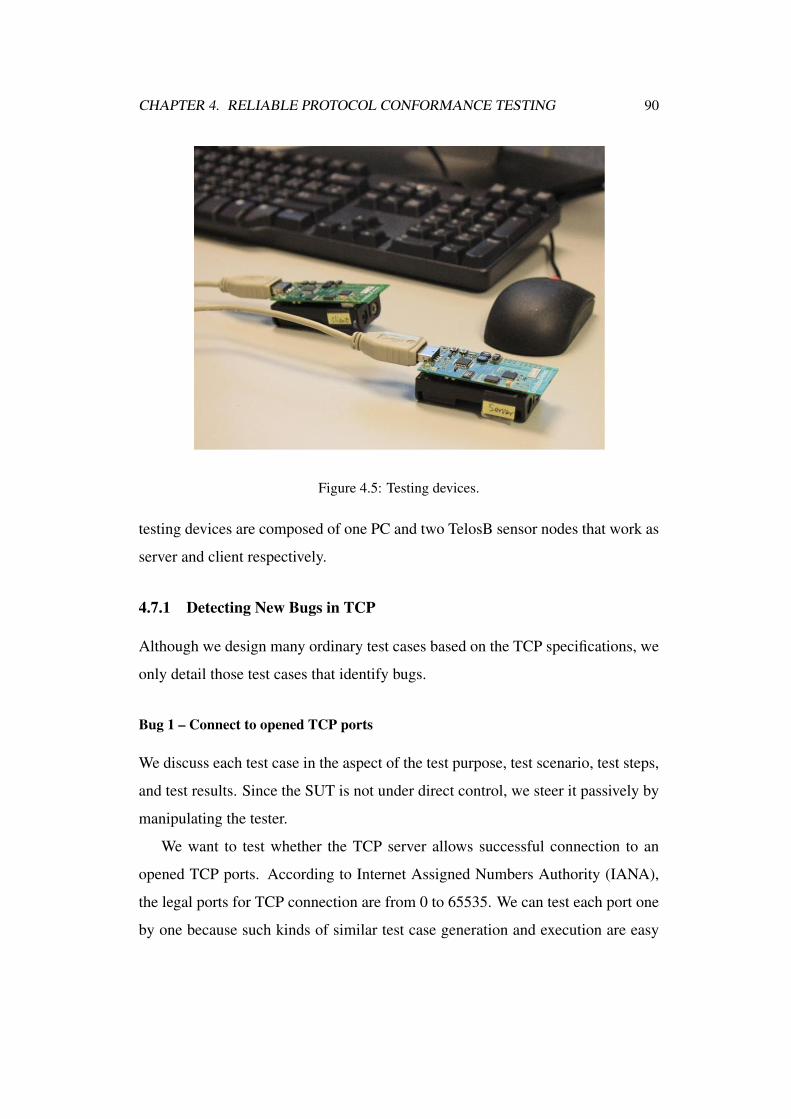
CHAPTER 4. RELIABLE PROTOCOL CONFORMANCE TESTING 90
Figure 4.5: Testing devices.
testing devices are composed of one PC and two TelosB sensor nodes that work as
server and client respectively.
4.7.1 Detecting New Bugs in TCP
Although we design many ordinary test cases based on the TCP specifications, we
only detail those test cases that identify bugs.
Bug 1 – Connect to opened TCP ports
We discuss each test case in the aspect of the test purpose, test scenario, test steps,
and test results. Since the SUT is not under direct control, we steer it passively by
manipulating the tester.
We want to test whether the TCP server allows successful connection to an
opened TCP ports. According to Internet Assigned Numbers Authority (IANA),
the legal ports for TCP connection are from 0 to 65535. We can test each port one
by one because such kinds of similar test case generation and execution are easy

CHAPTER 4. RELIABLE PROTOCOL CONFORMANCE TESTING 91
TCP client: 1025
[SYN/ACK
]seq=0,
ack=1
Sending SYN
SYN/ACK received,
sending ACK
ACK received,
connection stablished
[SYN]seq=0
[ACK]seq=1,ack=1
SYN received,
sending SYN/ACK
TCP server: 80
Figure 4.6: TCP three-way handshake.
to be automated, but it takes long time to execute. As a result, we choose several
representative ports to test. We select port 80 as a common port and port 0 as a
special port to test. Then we get two test cases.
Test case 1 – Test purpose: Connection to an opened common TCP port should
be successful.
Test scenario: TCP is the IUT. One sensor node is the SUT, and it functions
as the TCP server installed with the IUT. The UT runs on top of the IUT. It is a
simple application which just receives packets and sends the received packets to
the peer. The other node is the tester, in which the LT (or tester) is installed with
the test case. It functions as the TCP client.
Test steps: The testing steps are as the three-way handshake process of TCP
as shown in Fig. 4.6. First, the server opens port 80 and waits for connection.
Second, the tester sends an SYN packet to port 80 of the SUT. Then it waits for
the SYN/ACK packet from the SUT. If it does not receive the packet, it declares
the failure of the test and exits. Otherwise, it checks the content of the packet. If
the content is incorrect, it claims test failure. Otherwise, it replies an ACK packet
to the SUT and asserts test case pass.
Our method is different from KleeNet [102] in that only the node to be tested
is installed with the IUT. The other node is installed with test cases. Each test case
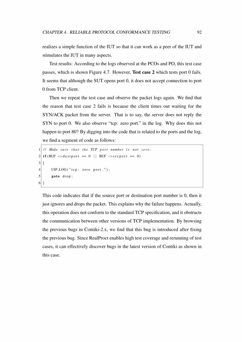
CHAPTER 4. RELIABLE PROTOCOL CONFORMANCE TESTING 92
realizes a simple function of the IUT so that it can work as a peer of the IUT and
stimulates the IUT in many aspects.
Test results: According to the logs observed at the PCOs and PO, this test case
passes, which is shown Figure 4.7. However, Test case 2 which tests port 0 fails.
It seems that although the SUT opens port 0, it does not accept connection to port
0 from TCP client.
Then we repeat the test case and observe the packet logs again. We find that
the reason that test case 2 fails is because the client times out waiting for the
SYN/ACK packet from the server. That is to say, the server does not reply the
SYN to port 0. We also observe “tcp: zero port.” in the log. Why does this not
happen to port 80? By digging into the code that is related to the ports and the log,
we find a segment of code as follows:
1 / / Make s u r e t h a t t h e TCP p o r t number i s n o t z e r o .
2 i f (BUF −>d e s t p o r t == 0 | | BUF −>s r c p o r t == 0)
3 {
4 UIP LOG ( ” t c p : z e r o p o r t . ” ) ;
5 goto drop ;
6 }
This code indicates that if the source port or destination port number is 0, then it
just ignores and drops the packet. This explains why the failure happens. Actually,
this operation does not conform to the standard TCP specification, and it obstructs
the communication between other versions of TCP implementation. By browsing
the previous bugs in Contiki-2.x, we find that this bug is introduced after fixing
the previous bug. Since RealProct enables high test coverage and rerunning of test
cases, it can effectively discover bugs in the latest version of Contiki as shown in
this case.
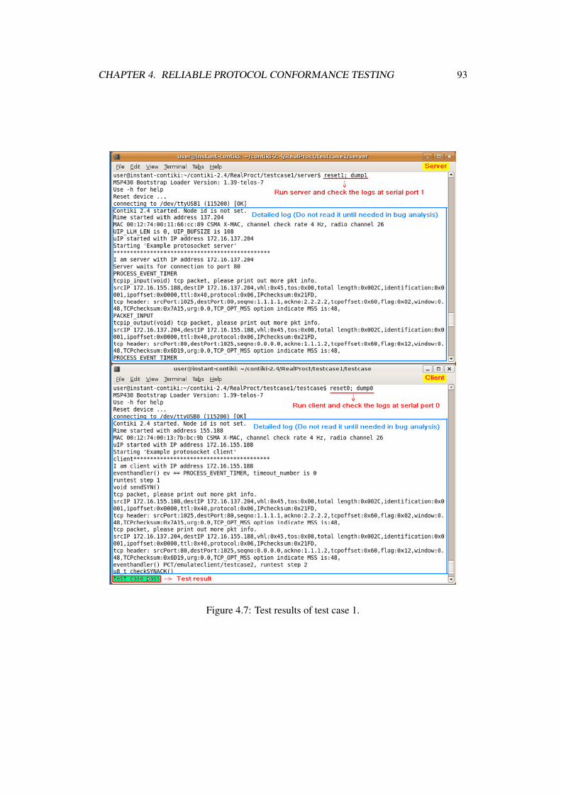
CHAPTER 4. RELIABLE PROTOCOL CONFORMANCE TESTING 93
Figure 4.7: Test results of test case 1.

CHAPTER 4. RELIABLE PROTOCOL CONFORMANCE TESTING 94
Bug 2 – Connect to unopened TCP ports
To complement the previous aspect of port testing in TCP, we should test whether
the TCP server allows successful connection to an unopened TCP ports. According
to the specification, if the client connects to an unopened TCP ports, the server
should reply a reset packet. Similarly, we also test two ports with two test cases.
Test case 3 – Test purpose: Connection to an unopened normal TCP port
should be unsuccessful.
Test scenario: It is the same as test case 1.
Test steps: First, the server opens port 80 and waits for connection. Second,
the tester sends an SYN packet to port 79 of the SUT. Then it waits for SYN/ACK
packet from the SUT. If it does not receive an RST packet from the server, it
declares the failure of the test and exits. Otherwise, it checks the content of the
packet. If the content is incorrect, it claims test failure. Otherwise, it asserts test
case pass.
Test results: pass. However, Test case 4 in which the client connects to port 0
of the server fails because it gets no RST reply after sending SYN. The reason is
the same as the previous bug. A mistake made in the program may result in more
than one failure in execution. Since the test execution in RealProct can be easily
automated, we would suggest software engineers to rerun the test cases after fixing
the bugs.
4.7.2 Detecting Previous Bugs in TCP
Apart from the new bugs, RealProct also detects the four old bugs discovered by
KleeNet earlier in the TCP stack implementation of Contiki [102]. The test cases
for discovering them are very short and simple. Hence, we only discuss the test
cases that identify the bugs caused by non-deterministic events because these bugs
will invoke our virtualization techniques.
According to the TCP specifications, packet loss leads to retransmission. As
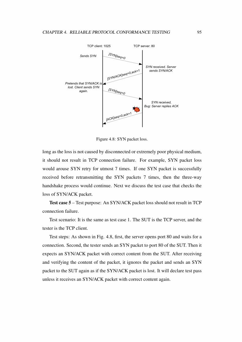
CHAPTER 4. RELIABLE PROTOCOL CONFORMANCE TESTING 95
TCP client: 1025
[SYN/ACK
]seq=0,a
ck=1
Sends SYN
Pretends that SYN/ACK is
lost. Client sends SYN
again.
[SYN]seq=0
[SYN]seq=0
SYN received. Server
sends SYN/ACK
TCP server: 80
SYN received,
Bug: Server replies ACK
[ACK]seq
=0,ack=1
Figure 4.8: SYN packet loss.
long as the loss is not caused by disconnected or extremely poor physical medium,
it should not result in TCP connection failure. For example, SYN packet loss
would arouse SYN retry for utmost 7 times. If one SYN packet is successfully
received before retransmitting the SYN packets 7 times, then the three-way
handshake process would continue. Next we discuss the test case that checks the
loss of SYN/ACK packet.
Test case 5 – Test purpose: An SYN/ACK packet loss should not result in TCP
connection failure.
Test scenario: It is the same as test case 1. The SUT is the TCP server, and the
tester is the TCP client.
Test steps: As shown in Fig. 4.8, first, the server opens port 80 and waits for a
connection. Second, the tester sends an SYN packet to port 80 of the SUT. Then it
expects an SYN/ACK packet with correct content from the SUT. After receiving
and verifying the content of the packet, it ignores the packet and sends an SYN
packet to the SUT again as if the SYN/ACK packet is lost. It will declare test pass
unless it receives an SYN/ACK packet with correct content again.

CHAPTER 4. RELIABLE PROTOCOL CONFORMANCE TESTING 96
Test results: fail. The reason is that the TCP server replies an ACK packet
to the TCP client at the second time when it receives an SYN packet. However,
the correct behavior for the TCP server is to send an SYN/ACK packet with right
content according to the specification. This error leads to two bugs discovered
earlier by KleeNet, which are also easily identified by RealProct. As long as this
error is fixed, multiple failures can be solved. Compared with KleeNet which has
to explore many redundant paths and manually write many assertions, our test
cases are clearer, more concise, and more specific. Besides virtualizing packet
loss flexibly, we can also generate extra test cases easily by retransmitting the
SYN packets from 2 times up to 6 times on Contiki-2.4 to verify whether this bug
is completely fixed. The results show that the above test cases all pass.
Similarly, we also design a test case that virtualizes SYN packet duplication
event to uncover a bug. The process is shown online1.
The next test case process utilizes event virtualization to virtualize SYN
packet duplication. It is true that the SYN duplication happens in practical TCP
communications. For example, the client sends a SYN packet to the server, but it
does not receive SYN/ACK in time. Hence it retransmits the SYN packet. The
second SYN is still on its long way to the server while the client receives the
SYN/ACK for the first SYN and replies the server an ACK packet. Due to the long
route the second SYN takes, it arrives at the server after the ACK. This process
is different from the virtualized process as shown in Fig. 4.9. Although the client
would not send another SYN to the server after establishing connection as shown in
Fig. 4.9, this virtualization is correct because the tester generates the same effects
as the practical process at the SUT. That is the SUT receives a duplicate SYN after
established connection. What’s more, this sequence of virtualized events is easy
to be produced and controlled by the tester.
Test case 6: Test purpose: A SYN duplicate should not result in TCP1http://www.cse.cuhk.edu.hk/˜jjxiong/testcases/testcase.htm
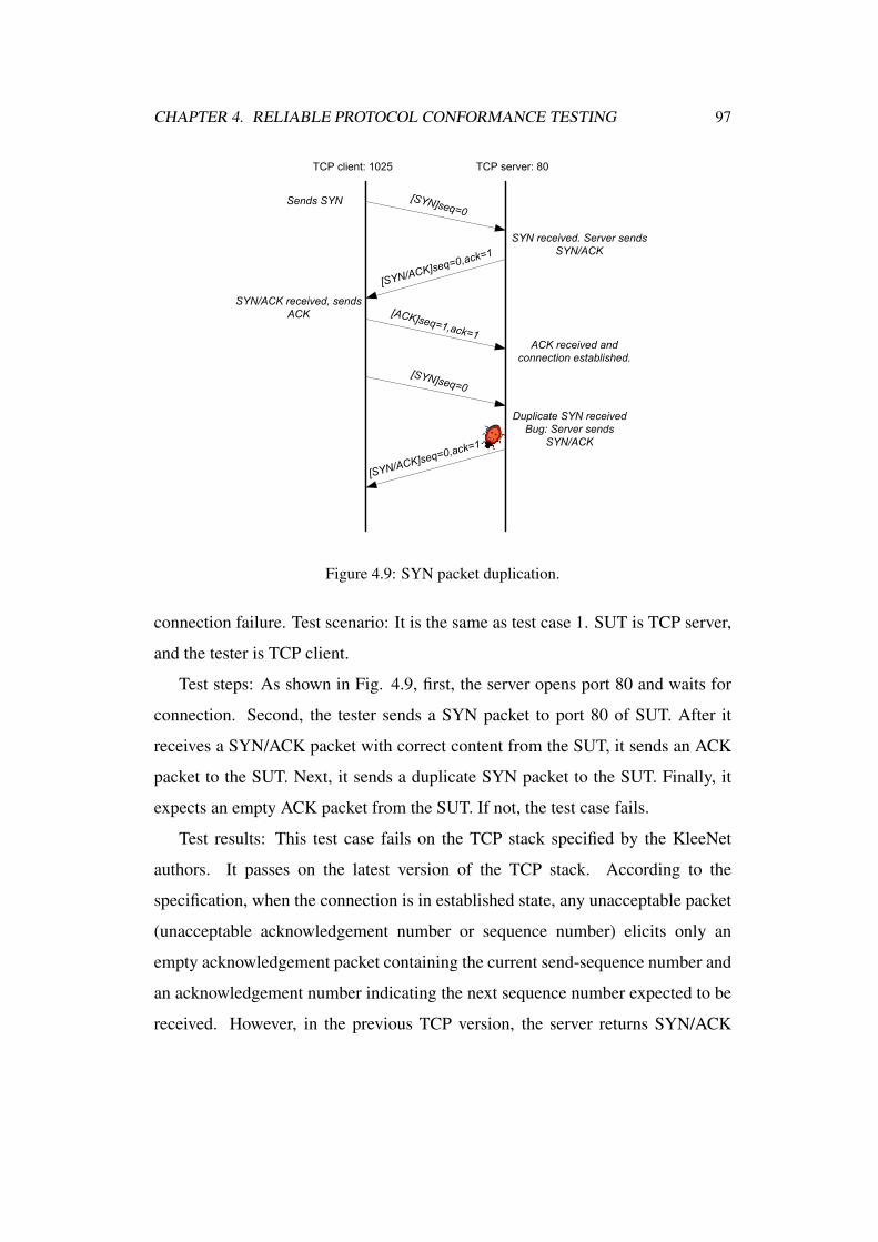
CHAPTER 4. RELIABLE PROTOCOL CONFORMANCE TESTING 97
TCP client: 1025
[SYN/ACK
]seq=0,a
ck=1
Sends SYN
SYN/ACK received, sends
ACK
[SYN]seq=0
[ACK]seq=1,ack=1
SYN received. Server sends
SYN/ACK
TCP server: 80
ACK received and
connection established.
[SYN/ACK
]seq=0,a
ck=1
[SYN]seq=0
Duplicate SYN received
Bug: Server sends
SYN/ACK
Figure 4.9: SYN packet duplication.
connection failure. Test scenario: It is the same as test case 1. SUT is TCP server,
and the tester is TCP client.
Test steps: As shown in Fig. 4.9, first, the server opens port 80 and waits for
connection. Second, the tester sends a SYN packet to port 80 of SUT. After it
receives a SYN/ACK packet with correct content from the SUT, it sends an ACK
packet to the SUT. Next, it sends a duplicate SYN packet to the SUT. Finally, it
expects an empty ACK packet from the SUT. If not, the test case fails.
Test results: This test case fails on the TCP stack specified by the KleeNet
authors. It passes on the latest version of the TCP stack. According to the
specification, when the connection is in established state, any unacceptable packet
(unacceptable acknowledgement number or sequence number) elicits only an
empty acknowledgement packet containing the current send-sequence number and
an acknowledgement number indicating the next sequence number expected to be
received. However, in the previous TCP version, the server returns SYN/ACK
CHAPTER 4. RELIABLE PROTOCOL CONFORMANCE TESTING 98
packet rather than replies an empty ACK packet. KleeNet identifies this bug from
the connection failures introduced by it. Unlike KleeNet, our method is quite direct
at the root cause. It does not analyze what kinds of failures this bug would further
introduce, and it is unnecessary to do so.
4.7.3 Testing Routing Protocol RMRP
For RMRP testing, we give two test cases demonstrating the topology
virtualization techniques presented in Section 4.5. The first test case checks
whether the SUT can establish route to 1-hop neighbor in the topology shown
in Fig. 4.4.
Test case 7 – Test purpose: The SUT can establish route to 1-hop neighbor 2.
Test scenario: RMRP is the IUT. One sensor node is the SUT, and it functions
as the route discovery originator installed with the IUT. The UT runs on top of the
IUT. It is a simple application that just receives packets and sends the received the
packets to the tester. The other node is the tester, in which the LT is installed with
the test case. It functions as all the other nodes in the topology.
Test steps: First, the SUT broadcasts a route request packet (REQ) before
sending a data packet to node 2. Second, the tester virtualizes node 2 to uni-cast
a route reply packet (REP) to the SUT and then virtualizes node a to forward
the REQ. Third, tester virtualizes node 2 to wait for the data from the SUT. On
receiving the data, it will declare test pass. Otherwise, it will assert failure.
Test results: The pass result validates the RMRP in aspect of route discovery
with 1-hop neighbor.
The second test case tests if the SUT can establish route to non-neighboring
nodes in the topology shown in Fig. 4.4. Since this topology will result in four
scenarios. The test case is divided into four sub-cases. We also show one sub-case.
Test case 8 – Test purpose: The SUT can establish route to non-neighboring
nodes d.

CHAPTER 4. RELIABLE PROTOCOL CONFORMANCE TESTING 99
Test scenario: It is the same as test case 7.
Test steps: First, the SUT broadcasts an REQ before sending a data packet
to node d. Second, the tester virtualizes node 2 to forward the REQ and then
virtualizes node a to forward the REQ. Third, after a while, tester virtualizes node
2 to uni-cast the REP originated from node d to the SUT. Finally, tester virtualizes
node d to wait for the data from the SUT. The next-hop of the data should be node
2. If it receives the data, it will declare test pass. Otherwise, it will assert failure.
Test results: The pass result validates the RMRP implementation in aspect of
route discovery and initiation with non-neighboring nodes.
4.8 Conclusions
In this chapter, we presented RealProct, a reliable protocol conformance
testing approach using real sensor nodes to check the conformance of protocol
implementation to the specification. RealProct includes two real sensor nodes
and a PC for testing and three techniques are carefully designed to support the
resource-limited sensor nodes. We proposed topology virtualization as a technique
for the two sensor nodes to imitate larger WSNs with different topologies, which
allows efficient and flexible protocol conformance testing. Event virtualization is
also invented to generate non-deterministic events to support virtualized topology
with multi-hop routing. We further enhanced the efficiency of testing and
the accuracy of verdict by determining the optimal number of test executions,
while guaranteeing an acceptable probability of false negative and positive
errors. We implemented RealProct in real sensor nodes and tested the protocol
implementation of the µIP TCP/IP stack in Contiki-2.4. RealProct effectively
found two new bugs and all the previously detected bugs in the µIP TCP/IP stack.
The experiments demonstrated that our protocol conformance testing setup can
effectively detect bugs that might be missed in simulations. We also tested and
validated the protocol implementation of Rime mesh routing in Contiki-2.4. The

CHAPTER 4. RELIABLE PROTOCOL CONFORMANCE TESTING 100
results indicated that RealProct can provide a cost-effective and flexible solution
for testing different advanced protocols, like multi-hop routing, which are more
sensitive to the network topology and the non-deterministic events in real wireless
channels.
Due to the limited number of real sensor nodes used, there are some cases that
RealProct cannot virtualize with high similarity. For example, It cannot virtualize
the wireless environment when interference caused by simultaneous transmissions
happens, although the result of interference is easy to be virtualized as packet loss
or erroneous packet. In the future, we will attempt at solving the problem with
more real sensor nodes.
2 End of chapter.
Chapter 5
Mobility-assisted Diagnosis for
WSNs
Though widely employed in various applications, WSNs are liable to failures,
especially after deployment. Since the on-site failures are difficult to reproduce, it
is of critical importance to perform in-situ diagnosis. Current in-situ diagnosis
methods are either intrusive or inefficient, because they either inject diagnosis
agents into each sensor node or build up another network for diagnosis purpose.
To tackle these issues, we propose MDiag, a Mobility-assisted Diagnosis approach
that employs smartphones to patrol the WSNs and diagnose failures. Diagnosing
with a smartphone which is not a component of WSNs does not intrude the
execution of the WSNs. Moreover, patrolling the smartphone in the WSNs to
investigate failures is more efficient than deploying another diagnosis network.
Statistical rules are designed to guide the detection of abnormal cases. Aiming at
improving the patrol efficiency, a patrol approach MSEP is proposed. MSEP is
designed to achieve better performance than the naive method, the greedy method,
and the baseline method in increasing the detection rate and reducing the patrol
time of MDiag. Experiments with real sensor nodes and emulations validate the
effectiveness of MDiag in detecting anomalous cases caused by faults.
101

CHAPTER 5. MOBILITY-ASSISTED DIAGNOSIS FOR WSNS 102
5.1 Introduction
Recently, many efforts have been devoted to improve the reliability of WSNs in
various aspects, such as simulation [68], debugging [132], and most importantly
in-situ diagnosis that observes real-time network status and enables timely
network failure detection [95]. WSNs are liable to failures, especially after the
deployment [66]. In addition, on-site failures are difficult to reproduce [77].
Hence, it is critical to perform in-situ diagnosis.
One in-situ diagnosis approach is to implant diagnosis agents into each sensor
node [95]. However, many already-deployed WSNs are not facilitated with
diagnosis functions [66]. We have to update the software of the whole WSN
so as to embed the diagnosis agents. Nevertheless, programming the agent into
each sensor node will inevitably affect the normal execution of a running WSN
application [48] [50]. In addition, the diagnosis agent in each sensor node is
usually required to transmit specified metrics back to a centralized station for
diagnosis. In a sensor node with limited resources, such diagnosis affects the
on-site application performance by consuming the bandwidth and the related
resources [95]. Furthermore, as we know, the execution of logging statements
could change the actual execution of a system and then may introduce bugs [98].
It is very costly to insert agents at each protocol layer although this would result in
high granularity diagnosis. How many agents to insert is a similar problem. The
more the agents are embedded, the more logs the diagnosis can obtain, and the less
efficient and more intrusive the diagnosis is.
To avoid the intrusion caused by agent injection, some approaches deploy
another network (such as another WSN) to monitor a WSN, but this approach is
neither efficient nor cost-effective. SNTS deploys several monitoring sensor nodes
(they formulate a snooping network) in the real field along with the original sensor
nodes [58]. The monitoring sensor nodes sniff and record the packets sent from the
monitored sensor nodes, which are manually retrieved to a PC for investigation.

CHAPTER 5. MOBILITY-ASSISTED DIAGNOSIS FOR WSNS 103
Figure 5.1: A MDiag patrol scenario. The smartphone first visits sensor node 1, then
sensor node 2, 3, 4, and 5.
For a large WSN, SNTS needs to deploy many monitoring sensor nodes; as a
result, SNTS does not adapt to large WSNs well. SNIF deploys a temporary
wireless network to snoop a WSN [100]. It is better than SNTS in that it does
not need to manually fetch back the monitoring nodes, but its nodes are required
to be equipped with two radio sets.
To tackle the above disadvantages, we are the first to propose a
mobility-assisted diagnosis (MDiag) approach to examine failures in WSNs with
an independent mobile device. Nowadays, mobile smartphones are increasingly
popular. By the end of 2011, there are 6 billion mobile subscribers globally, and
smartphone users show the strongest growth [2]. It is now convenient to patrol
a deployed WSN with smartphones to collect packets sent from sensor nodes.
Then the smartphones can perform diagnosis by analyzing these packets. Such
a diagnosis process can be flexibly turned on or off, allowing users to perform an

CHAPTER 5. MOBILITY-ASSISTED DIAGNOSIS FOR WSNS 104
on-demand diagnosis. For WSNs that are deployed in harsh areas without human
traces, mobile robots are able to carry the smartphones.
A diagnosis scenario with one smartphone is shown in Figure 5.1, where
the dotted lines are the patrol path of the smartphone. The smartphone starts
snooping sensor node 1 for a certain interval, continues traveling along the path
and snooping sensor nodes 2, 3, 4, and 5 for some intervals, and then returns to the
starting sensor node 1.
The most important feature of such an approach is that it is not intrusive to
WSN applications because the smartphones themselves are not components of
WSNs. MDiag does not need to implant diagnostic agents to the applications,
and thus it does not need to modify the applications as the proactive approaches
do. Hence, MDiag can be employed to scrutinize any deployed WSNs when
needed without affecting the WSN performance. In addition, the mobility of
smartphones allows users to apply one or several smartphones to record the packets
sent from the WSN instead of many debugging sensor nodes that need laborious
manual placement and retrieval. Finally, MDiag can collect all kinds of raw
packets (packet created from the radio frequency chip that contains packet header
information of the upper layer protocols), which is especially useful in finding
more failures. To analyze raw packets of all types, the agent approaches need
to inset agents at all the protocol agents, which is very inefficient. For example,
MDiag can collect control packets exchanged locally, which are not transmitted
back to the BS for diagnosis in Sympathy [95].
The design of MDiag mainly faces two challenges. First, it is difficult to
determine the abnormal behaviors from the collected various packets, such as
routing packets, MAC layer control packets, and application data packets. We
define a few statistical rules to identify anomalies based only on minimum prior
knowledge of the system. Second, the patrol pattern of the smartphones influences
the failure detection rate. How to design the patrol method for visiting the
CHAPTER 5. MOBILITY-ASSISTED DIAGNOSIS FOR WSNS 105
sensor nodes in order to collect packets is crucial and difficult. We propose a
method called MSEP (maximum snooping efficiency patrol) which identifies the
sensor node set to patrol and collect relevant packets for analysis. Consequently,
it increases the failure detection rate. Finally, in comparison with the naive
method, greedy method, and baseline method, we perform extensive experiments
to demonstrate the effectiveness of MDiag and show its effective detection of
several interesting failures.
The rest of this chapter is organized as follows. First, Section 5.2 highlights
the related work. Next, Section 5.3 clarifies the network architecture and failure
classification for MDiag. Section 5.4 designs the framework of MDiag while
Section 5.5 proposes the algorithm for the smartphone patrol approaches. Section
5.6 presents the results of our experimental evaluation. Finally, Section 5.7
concludes the chapter.
5.2 Related Work
There has been tremendous work in finding faults that will cause network
failures in WSNs. Some of them are based on simulations, such as ns-3 [3],
a general network simulator, and TOSSIM [68], a simulator for WSNs running
on TinyOS [69]. More advanced simulation-based failure detection tools include
T-Check [72] and KleeNet [102]. T-Check [72] is an event-driven simulator
developed from TOSSIM, while KleeNet [102] is based on the low-level symbolic
virtual machine. Given the fact that the behaviors of nodes in a simulation
environment and real sensor nodes are not the same, in-situ diagnosis approaches
for WSNs are indispensable.
One kind of in-situ diagnosis approaches is to embed diagnosis agents into
each sensor node. For example, by injecting the diagnosis agent, Sympathy [95]
actively collects run-time status from sensor nodes, such as routing table and
flow information, and detects possible faults after transmitting them to the BS.
CHAPTER 5. MOBILITY-ASSISTED DIAGNOSIS FOR WSNS 106
Nevertheless, these approaches are not adaptable for WSNs that have already
been deployed without such agents. Because we have to update the software of
WSNs so as to embed the agents, this unavoidably affects the running of WSN
applications [50]. Moreover, Sympathy asserts that it only employs one rule that
insufficient data at the BS imply failures, which means that it cannot detect certain
network failures, such as overenthusiastic transmission which results in reduced
battery lifetime.
For WSNs deployed with these diagnosis agents, the agent injection methods
inevitably intrude the WSN applications. The agent execution may cost extra
CPU computation, communication bandwidth, and energy of the sensor nodes,
which imposes heavy burden on the resource-limited networks. Since Sympathy
costs extra communications bandwidth and energy consumption in order to
actively transmit the information, PAD [75] and PassiveAssertions [101] reduce
the diagnosis efforts by piggybacking the logs in regular data packets. Agnostic
Diagnosis [81] also needs to collect enough amount of network state information to
perform agnostic diagnosis. Self-Diagnosis [76] involves multiple local nodes in
cooperation to detect WSN failures based on finite state machines. This approach
reduces the communications effort of transmitting the logs to the BS. Since all the
existing in-situ diagnosis approaches are intrusive to the WSNs, we propose a new
MDiag approach. Instead of changing the WSN systems, MDiag employs mobile
phones to travel in deployed WSNs and to passively collect raw packets sent from
the passing sensor nodes. The collected packets can then be utilized for diagnosis.
Because mobile phones are not a part of WSNs, MDiag does not intrude the WSNs
and is thus adaptable to all WSN applications.
Another type of approaches to avoid the intrusion to WSN applications is
deploying another network to monitor the WSN. SNTS deploys several monitoring
sensor nodes in the real field along with the original sensor nodes [58]. The
monitoring sensor nodes sniff and record the packets sent from the sensor nodes

CHAPTER 5. MOBILITY-ASSISTED DIAGNOSIS FOR WSNS 107
that they observe. Although the debugging sensor nodes can formulate a network,
they cannot communicate with each other and transmit the recorded packets to the
BS because their transmissions would cause interference to the original WSN. As
a result, in fetching the recorded packets, all of the debugging sensor nodes have
to be manually retrieved, which is quite labor-intensive. In addition, for a large
WSN, SNTS should deploy many debugging sensor nodes so as to guarantee that
all the original sensor nodes can be monitored; hence SNTS does not suit large
WSNs.
To avoid the efforts of manually retrieving the nodes in the monitoring
network, SNIF deploys a different monitoring network which is composed of
nodes with two sets of radio equipment [100]. One set is used to passively listen
to the packets sent from the WSN. The other set employs a different wireless
channel to transmit the sniffed packets to the BS without interfering the original
WSN. Nevertheless, dual radios are generally not facilitated in the off-the-shelf
sensor network products. Moreover, like SNTS, SNIF also deploys an additional
diagnosis network, which is not cost-effective. With our MDiag approach, the
mobility of diagnosis devices saves the cost of the large monitoring network
deployment, and the employment of smartphones eliminates the extra hardware
requirement of monitoring nodes.
Finally, mobile sensor nodes have already been introduced to improve WSN
coverage [74] [125] while multiple, mobile base stations are also deployed to
prolong the lifetime of the WSNs [106] [126]. In the recent innovative application
OppSense [84], the mobile phones are the users while the WSN is a service
provider. However, no prior work has employed mobile platforms, such as the
smartphones, for diagnosing WSNs. MDiag is the first work to utilize mobile
platforms for WSN diagnosis purpose.

CHAPTER 5. MOBILITY-ASSISTED DIAGNOSIS FOR WSNS 108
5.3 MDiag Background
5.3.1 Network Architecture
We consider a network which involves a BS and static wireless sensor nodes
deployed in a sensing field for monitoring temperature, humidity, noise level,
etc., from the environment. A smartphone is able to receive the raw packets sent
from the sensor nodes within its reception range as long as it is equipped with
the same reception device as the sensor nodes or it is attached with a sensor node
for snooping purpose only [84] [97]. To diagnose, the smartphone can patrol in
the WSN field as shown in Figure 5.1. The patrol can start at any time and last
for any duration according to the requirement of WSN maintainers. For example,
they may want to patrol a WSN once each day, or they only turn on the diagnosis
for a long period when they need to ascertain and find more information about
suspicious phenomena.
Intuitively, the more the smartphones are available for WSN diagnosis, the
better the diagnosis effectiveness is. Nevertheless, more efforts are required to
carry them in the network field. Without loss of generality, in the following we
discuss the case of using one smartphone to patrol a WSN and to passively collect
network packets. The case of using more smartphones can be similarly extended.
5.3.2 Failure Classification
MDiag is proposed to diagnose the failures in WSNs by collecting and analyzing
the packets sent by sensor nodes. Since it can only diagnose the network failure
according to the packets sent out in the WSNs, it cannot detect failures that are not
triggered during the execution. The failures are divided into three classes as shown
in Figure 5.2. The x-axis is failure lasting time, and it increases from left to right.
The first class is transient failures that last for a very short period, such as random
packet loss considered in [135]. The second class lasts only for a longer period and

CHAPTER 5. MOBILITY-ASSISTED DIAGNOSIS FOR WSNS 109
Figure 5.2: Failure classification.
then disappears, such as routing failures, link failures, and congestion. It is called
short-term failure. The third class is permanent failures that stay in the network
until they fixed or they stay for a very long time, such as node crash and incorrect
resource allocation failures. We discuss some of the failures we identified in our
experiments in Section 5.6.
The transient failures hold for a very short time and they do not affect the
network behaviors distinctively, so we can hardly detect them by in-situ diagnosis.
In the following, we focus on detecting the permanent failures and short-term
failures.
5.4 MDiag Framework
Referring to the diagnosis scenario shown in Figure 5.1, we design the MDiag
framework as shown in Figure 5.3.
In the first step, by visiting each sensor node in the WSN for a sufficiently long
time, the smartphone can get the neighboring information of each sensor node. It
inputs the neighboring information to the algorithm of patrol set selection which
generates the set of K sensor nodes to patrol. Note that we do not need to know
the WSN topology, although during the patrol the smartphone could build up a
coarse topology by locating each sensor node’s approximate position with its GPS
equipment. During the initial WSN visit, we can also estimate the traffic load at
each sensor node. Then the time that the smartphone stays along with each sensor
node in the patrol set is easy to be calculated. The heavier the traffic load, the
shorter the time that the smartphone requires to collect enough data packets and
other control packets for the statistical analysis.

CHAPTER 5. MOBILITY-ASSISTED DIAGNOSIS FOR WSNS 110
Raw packets
collected by the
smartphone
Statistical results on raw packets
K sensor nodes to
be patrolled
Statistical rules
on packet
analysis
Packet
sequencePacket
decoder in the
smartphone
Algorithm of patrol
set selection
Packet
structures
WSN developers
(or specifications)
Problem report
Step 1Step 2
Step 3
Figure 5.3: MDiag framework.
In the second step, on the basis of packet structures provided by WSN
developers or system specifications, packet decoder and some statistical rules for
packet analysis are applied on the collected packets.
In the third step, the sequence of packets collected during the patrol of the K
sensor nodes is input to the packet decoder, which will generate statistical results.
Based on the statistical rules on packet analysis, if the smartphone deducts that
the network behavior is abnormal, it can produce a failure report and trigger
the additional diagnosis. Further actions, such as collecting extra packets for
more detailed inspection, can be taken to analyze the phenomenon and locate the
potential bugs.
Next we focus on the input and output of the packet decoder and the statistical
rules on packet analysis. The algorithm of patrol set selection will be discussed in
the next section.
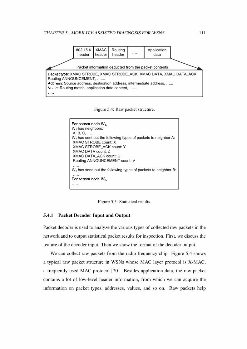
CHAPTER 5. MOBILITY-ASSISTED DIAGNOSIS FOR WSNS 111
Figure 5.4: Raw packet structure.
Figure 5.5: Statistical results.
5.4.1 Packet Decoder Input and Output
Packet decoder is used to analyze the various types of collected raw packets in the
network and to output statistical packet results for inspection. First, we discuss the
feature of the decoder input. Then we show the format of the decoder output.
We can collect raw packets from the radio frequency chip. Figure 5.4 shows
a typical raw packet structure in WSNs whose MAC layer protocol is X-MAC,
a frequently used MAC protocol [20]. Besides application data, the raw packet
contains a lot of low-level header information, from which we can acquire the
information on packet types, addresses, values, and so on. Raw packets help

CHAPTER 5. MOBILITY-ASSISTED DIAGNOSIS FOR WSNS 112
us analyze the network behaviors from all protocol layers, including interactions
between layers.
The input of the packet decoder is a sequence of raw packets. After decoding
the raw packets according to the structures shown in Figure 5.4, the output is
statistical results for the failure report shown in Figure 5.5. It shows the sensor
node neighbor information, the count of each type of packets, and so on.
5.4.2 Statistical Rules on Packet Analysis
The aforementioned rules describe statistical packet behaviors in WSNs; therefore,
they are not applicable to analyze a single packet exchange process. For example,
the rules cannot be used in detecting the failure of the TCP three-way handshake
caused by random packet loss because a TCP three-way handshake process
does not compose a statistical packet behavior [24]. Moreover, a random TCP
packet loss does not mean application failure or performance degradation unless it
happens frequently.
Because our rules are statistical and are provided by the developers or based
on the specification, they are a subset of the specification-based rules as shown
in Table 5.1. Unlike the state-of-the-art approach Sympathy [95] which employs
only one rule, i.e., insufficient data at the BS imply failures, our statistical rules
are based on the targets of all protocol layers. Hence our approach can detect more
failures than Sympathy [95].
By decoding the raw packet, we can infer the following packet fields on which
the statistical rules utilize:
• Packet type
• Packet count of each type
• Packet directions
• Neighbor information

CHAPTER 5. MOBILITY-ASSISTED DIAGNOSIS FOR WSNS 113
Table 5.1: Our statistical rules are a subset of the specification-based rules.
Layer Specification-based rules Statistical
rules
Application layer
The value (e.g., temperature) of the application data falls within
the range specified.
Yes
The number of data packets exchanged among the BS and the
sensor nodes should be within the specified range in a certain
interval.
Yes
The data communication process (such as the packet order) is
based on the specification.
No
...
Routing layer
The routing metric value is in the specified legal range. Yes
The number of each kind of routing packets sent out by the BS
and sensor nodes is normal within a certain period.
Yes
The routing packet exchange sequence should conform to a
specific routing protocol (e.g., first routing request packet, then
routing reply packet).
No
...
MAC layer
The number of each kind of MAC packets sent out by the BS
and sensor nodes is normal within a certain period.
Yes
The MAC packet exchange process is based on the
specification.
No
...

CHAPTER 5. MOBILITY-ASSISTED DIAGNOSIS FOR WSNS 114
• Packet value, such as the routing metric of a routing packet, data content of
an application data packet, and so on.
Without loss of generality, we take one kind of the most popular WSN applications,
the data gathering application, including routing protocol CTP [42] and X-MAC
protocol [20], as an example and give the major statistical rules in Table 5.2.
This set of rules can be extensible according to the statistical granularity. The
parameters used in the rules are represented in Figure 5.5.
Table 5.2: Statistical rules for a typical WSN application.
Layer Statistical rules
Application layer Rule 1. For BS, Z, the number of application data sent out, is 0.
Application layer Rule 2. For sensor nodes other than BS, Z is within the application requirement.
Routing layer Rule 3. For BS, the legal routing metric is 0.
Routing layer Rule 4. For sensor nodes other than BS, routing metric value is legal.
Routing layer Rule 5. For sensor nodes other than BS, no bidirectional data exchange exists, i.e.,
Z ∗ U = 0
MAC layer Rule 6. For sensor nodes other than BS, the number of each kind of MAC packets
sent is normal, i.e., Y ≃ U,X > or ≫ Z.
According to the application target, the data flow is only from the sensor nodes
to the BS, and hence we derive Rule 1 and 2 in Table 5.2. Rule 1 means that the BS
does not send data packets. Rule 2 means that other sensor nodes send the required
amount of data packets.
Based on the routing protocol target, Rule 3 and 4 clarify the legal range of
the routing metric, and Rule 5 means no routing fluctuation. There should be no
bidirectional data exchange between two sensor nodes; otherwise, it is possible
that the routing is unstable and causes the two sensor nodes to use each other as
the forwarding counterpart.
Rule 6 comes from the X-MAC behavior between a pair of communicating
CHAPTER 5. MOBILITY-ASSISTED DIAGNOSIS FOR WSNS 115
sensor nodes, i.e., for each sensor node, the number of X-MAC STROBE ACK
packets sent should be almost equal to the number of X-MAC DATA ACK packets
sent and the number of X-MAC DATA packets received. If Rule 6 is violated, say
the number of X-MAC STROBE ACK packets sent is far more than the number
of X-MAC DATA ACK packets sent, then the X-MAC works inefficiently.
The application mechanism, the CTP protocol, the X-MAC protocol should be
working well when these rules are satisfied. The BS receives its expected data
regularly, and the CTP and X-MAC protocols work efficiently without too much
extra energy consumption for communications.
5.5 Coverage-oriented Smartphone Patrol Algorithms
By patrolling the WSN, we can collect the packets sent out by the sensor nodes in
the patrol set. By analyzing these packets, we can diagnose the WSN. Collecting
more packets can help detect more failures. If the packets from some sensor nodes
are never collected, failures happening at these sensor nodes are less likely to be
discovered. As a result, the patrol approach should try to cover all the sensor nodes
in the WSN. Due to their different coverage efficiency, different patrol methods can
affect the detection efficiency, especially for the short-term failures.
We do not consider the cost during the travel, hence the visiting order of the
sensor nodes in the patrol set is not a concern in our patrol set establishment
process. The key is the patrol set rather than the patrol path. Moreover, our
experiments also verify that the difference is very small (less than 3% in most
cases) for visiting the sensor nodes in the same patrol set in different order.
5.5.1 Naive Method (NM)
The first method is the naive method that the smartphone visits all the sensor nodes
one by one, but it needs a long time to traverse the deployed WSN for only one
round. If a failure happens at the last sensor node that will be patrolled, it is

CHAPTER 5. MOBILITY-ASSISTED DIAGNOSIS FOR WSNS 116
Figure 5.6: Network topology I. The smartphone stays near sensor node 2.
very likely that when the smartphone finally arrives at the sensor node, the failure
phenomenon has already disappeared. Correspondingly, the failure detection rate
of NM is low. If we can cover all the sensor nodes in a shorter period, then the
failure missing rate would be lower.
5.5.2 Greedy Method (GM)
To reduce the patrol time, we utilize the broadcast nature of wireless transmissions
and thus design methods that perceive all the sensor nodes without visiting each
sensor node one by one. For example, in Figure 5.6, since node 2 is neighboring to
nodes 1 and 3, a smartphone that visits node 2 can also overhear the packets sent
from node 1 and node 3. As a result, to patrol all the senor nodes in this topology,
we only need to visit node 2 and node 4 instead of visiting all the 4 nodes one by
one. By patrolling the sensor nodes in the patrol set, all the sensor nodes could be
snooped without visiting them one by one.
However, to find the patrol set with the minimum sensor nodes is a set cover
problem, which is shown to be NP-complete [55]. An intuitive method is the
greedy method (GM) [54]. To simplify the GM explanation, we choose a regular
9-node network topology as shown in Figure 5.7, in which sensor node 1 is the
BS, and the other 8 nodes are sensor nodes. Sensor node 5’s neighbors are: 2, 4,
6, and 8. The degree of each sensor node v is the number of its neighbors, denoted
as Degree(v). For example, for sensor node 5, Degree(5)=4, and for sensor node
1, Degree(1)=2.

CHAPTER 5. MOBILITY-ASSISTED DIAGNOSIS FOR WSNS 117
Figure 5.7: Patrol set selection of GM (sub-figure a) and MSEP (sub-figure b). The blue
circle is put into the patrol set.
We define the snooping efficiency of visiting a sensor node v as Degree(v).
Visiting v can overhear the other (Degree(v)−1) sensor nodes. The larger the
snooping efficiency the better, because more packets can be collected on the visit.
The snooping efficiency of a patrol set S with K sensor nodes is defined as1K
∑v∈SDegree(v). Improving the patrol set snooping efficiency can increase the
packets collected for diagnosis, and hence raise the failure detection probability.
By them our target is to improve the patrol set snooping efficiency rather than to
solve the minimum set cover problem. When the sensor node coverage is satisfied,
minimizing the patrol set size can increase the patrol set snooping efficiency, and
increasing the patrol set snooping efficiency helps reduce the patrol set size.
In the GM algorithm, the smartphone always selects to visit the sensor node
whose current degree is the largest. Each time a sensor node is selected into the
patrol set, its neighbors and itself are removed from the neighbors of the remaining
sensor nodes. Hence, the degrees of the remaining sensor nodes are updated for
the next greedy selection. The sensor node selection continues until all the sensor
nodes can be snooped.

CHAPTER 5. MOBILITY-ASSISTED DIAGNOSIS FOR WSNS 118
5.5.3 Maximum Snooping Efficiency Patrol (MSEP)
GM can result in selecting several sensor nodes with small degree. For example,
the selection results with GM are shown in sub-figure (a) of Figure 5.7. Sensor
nodes 1, 3, 7, and 9 are visited with low snooping efficiency because their
degrees are 2. In contrast, sensor node 5 is visited with high snooping efficiency.
Nevertheless, since many sensor nodes are visited with low snooping efficiency,
GM cannot achieve high patrol set snooping efficiency which is 2.4. Eliminating
or reducing such visiting can help enhance the snooping efficiency and reduce the
patrol set size. Therefore, we design a different method called maximum snooping
efficiency patrol (MSEP) that can traverse all the sensor nodes with a smaller patrol
set size. In comparison, its patrol set selection of the regular 9-node network is
shown in sub-figure (b) of Figure 5.7, which contains only 3 sensor nodes rather
than 5 sensor nodes for the GM algorithm. The snooping efficiency of this patrol
set is 2.67, higher than that of GM patrol set.
MSEP aims at enhancing the snooping efficiency by reducing small degree
node selection probability. Therefore, it can correspondingly reduce the patrol
set size. On one hand, it should guarantee to cover every sensor node, including
the sensor node with a small degree. Therefore, MSEP first finds i, the sensor
nodes with the minimum degree. On the other hand, to reduce small degree node
selection probability, it selects a sensor node j with the largest degree from i’s
neighbor set. By visiting j, the smartphone can also snoop i, and the snooping
efficiency is increased. Then j is added to the patrol set M . Nevertheless, such
selection may still result in selecting sensor nodes with a small degree in the future.
Hence, MSEP rewinds and corrects sensor node j and i selection for a few times.
The details are shown in Algorithm 6.
The first step in Algorithm 6 is the sensor node selection and degree update. At
line 7, sensor node i with the minimum degree is selected. At line 14, sensor node
j with the largest degree is chosen to be included in the patrol set. To calculate
CHAPTER 5. MOBILITY-ASSISTED DIAGNOSIS FOR WSNS 119
how many sensor nodes remain to be patrolled, line 16 deletes j and sensor nodes
in its neighbor set Nj from S ′ and W ′. Corresponding to the deletion, line 17
updates the degree of the remaining sensor nodes in S ′ and W ′ (i.e., the degree is
decreased because of sensor node deletion).
Next is the refinement of sensor node selection. Line 19 checks whether
selecting j will result in the remaining sensor nodes with a small degree, e.g.,
degree 1. If the answer is no, we select the j and add it to M (line 22). Otherwise,
we refine the sensor node selection. We select a different j (back to line 14). If
all sensor nodes in Hi result in sensor nodes with a degree 1, remove i from S,
add it to W (line 20), and repeat to find a sensor node with the minimum degree
in S (back to line 7). Doing such check and sensor node selection refinement can
improve the snooping efficiency. In our algorithm we choose to refine the selection
of sensor nodes with degree 1. We can also refine with a larger degree, which can
improve the snooping efficiency, but will cost more computation efforts.
After handling all the sensor nodes in S, we visit the sensor nodes in W . The
difference is that when handling sensor nodes in W , we do not take refining actions
on sensor nodes with degree 1.
5.6 Evaluations
For permanent failure detection, we carry out the evaluations with 4 TelosB
sensor nodes and 1 Andriod smartphone [97]. We perform emulations on sensor
node operating system Contiki-2.4 [33] for short-term failure detection. In all
the experiments, an existing application, data collection application runs with
underlying routing protocol CTP [42] and X-MAC protocol [20]. We use real
failures encountered in our experiments and also failures found in the code
repositories of Contiki, and passively collect the raw packets sent from the radio
frequency chip. The received packets can be stored at the smartphone which is
equipped with larger memory. Then based on the packet format, we provide a

CHAPTER 5. MOBILITY-ASSISTED DIAGNOSIS FOR WSNS 120
Algorithm 6 MSEP algorithm.1: Node set S = {all the nodes}
2: Patrol set M = ∅
3: Candidate node set W = ∅
4: S′ = S,W ′ = W
5: k = 0 //k is the size of set M
6: while S != ∅ do
7: Choose a node i ∈ S with the minimum degree //from neighbor information
8: Let Hi = Ni∪
i// Ni is node i’s neighbor set
9: repeat
10: S′ = S,W ′ = W
11: if Hi == ∅ then
12: break
13: end if
14: ∀ nodes ∈ Hi, choose j with the largest degree
15: Delete j from Hi
16: Delete j and Nj from S′ and W ′
17: Update Degree(v), ∀v ∈ S′ and W ′
18: until Do not exists v ∈ S′ with Degree(v) == 1
19: if Hi == ∅ and ∃v ∈ S′ with Degree(v) == 1 then
20: Delete i from S, add i to W,W ′ = W,S′ = S
21: else
22: Add j to M,W = W ′, S = S′, k = k + 1
23: end if
24: end while
25: while W != ∅ do
26: Choose a node i ∈ W with the minimum degree
27: ∀ nodes ∈ Ni∪
i, choose j with the largest degree
28: Add j to M , Delete j and Nj from W,K = K + 1
29: Update Degree(v), ∀v ∈ W
30: end while

CHAPTER 5. MOBILITY-ASSISTED DIAGNOSIS FOR WSNS 121
packet decomposition program (small enough to fit in smartphones) to analyze the
received packets online and then generate the failure report.
Besides NM and GM, we also implement a baseline method called RM-K.
RM-K randomly selects K sensor nodes to form the patrol set. It does not care
whether such set can cover all the sensor nodes, i.e., visiting the sensor nodes in
the set can snooping all the sensor nodes in the WSN. We repeat the random patrol
set selection for 100 times and use the averaged results for RM-K.
5.6.1 Permanent Failure Detection
Initially, for the purpose of demonstrating an existing WSN application in Contiki,
we build up and run it with four telosB sensor nodes and one smartphone shown
in Figure 5.6. We do not expect any failure because the topology is simple and the
application is provided by the developers. However, the failure still happens.
Specifically, in the packets which sent from sensor node 2 to sensor node 3, the
ratio of X-MAC STROBE ACK packets to X-MAC DATA ACK packets is about
52, while in fact the ratio should be around 1 according to Rule 6. This means that
node 2 agrees to receive X-MAC DATA packets from node 3 for 52 times, but it
only tells node 3 that it receives the expected data packets once.
This is a performance degradation failure because it costs a lot of control packet
exchange to transmit one required data packet and the energy consumption is very
high. It can hardly be detected at the application layer because the BS receives
the expected data packets. Although this problem does not fail the application
in this simple topology, it will break down the application when the network size
increases. In this experiment, the smartphone can detect the failure by staying near
any sensor node. It finds that the collected packets violate Rule 6.
It is very surprising that this failure is caused by the ‘printf’ statements in the
application program. As we know, for the program running in the PC, inserting
a few ‘printf’ statements can hardly affect the normal execution. Nevertheless, it
CHAPTER 5. MOBILITY-ASSISTED DIAGNOSIS FOR WSNS 122
damages the WSN application execution. In this WSN application, every time a
sensor node is going to send out a data packet, it will first print out a message
‘Sending’. By analyzing the actual running process of the sensor node, we notice
that the ‘printf’ statement will issue the serial port interrupt, which will post
a process to print out a character. Printing out several characters means more
processes posted in the CPU queue. As a result, the ‘printf’ statement will take up
so many CPU resources that the CPU is too busy to handle the packet transmission
and reception in time. As a result, the packets are dropped after the sensor node
receives them at the physical layer rather than being dropped on the way.
Forgetting to comment out the debugging ‘printf’ statements is very common.
Writing redundant statements is also common, which may fail the WSN
applications due to consumption of limited resources. This kind of failures is
not easy to be identified because the programs are correct in the functional and
logical aspects. As performance degradation failure, they may not be manifested
in simple scenarios, such as in a small-scale testbed. Nevertheless, since MDiag
is able to collect raw packets of all types, it can analyze the WSN application and
detect failures at all protocol layers. In other words, it can help find failures that
do not just occur at the application layer.
5.6.2 Short-term Failure Detection
The patrol approaches are very crucial in detecting short-term failures. For the sake
of easy identification of correct behaviors, we use the regular network topology
shown in Figure 5.8. In fact, our MDiag also works very well with sensor nodes
randomly deployed because our algorithm of patrol sensor node set selection relies
only on neighbor information of each sensor node rather than on the precise
topology and locations.

CHAPTER 5. MOBILITY-ASSISTED DIAGNOSIS FOR WSNS 123
Figure 5.8: Network topology II. The smartphone patrols the sensor nodes in the network.

CHAPTER 5. MOBILITY-ASSISTED DIAGNOSIS FOR WSNS 124
600
800
1000
1200
1400
1600
1 2 3 4 5 6 7
Tim
e (
s)
Abnormal case number
Figure 5.9: Lasting time of the abnormal cases.
Short-term failure explanation
Next we run the existing application in a larger network shown in Figure 5.8. It is
composed of 25 sensor nodes with sensor node 1 as the BS. The smartphone patrols
the network with different patrol algorithms (NM, GM, MSEP, and RM-K).
We find that the routing is very unstable when the WSN starts to run. Many
bidirectional data exchange happens, which violates Rule 5. After a long time
the routing stabilizes, i.e., no bidirectional data exchange. Due to node crash and
application fix, sensor node reboot is not rare in real deployment. We reboot a
sensor node during the application running process. Because such reboot takes a
very short time, according to the basic mechanisms of routing protocol CTP, we
expect that the routing may remain unchanged or the routing of the surrounding
sensor nodes may change a little. Nevertheless, the reboot results in routing
fluctuation in a large range and for a long time. Rule 5 is violated again, i.e.,
bidirectional data exchange happens.
This failure in the routing protocol CTP is caused by not initializing the routing
value of each sensor node to the maximum value while the routing value of the BS
CHAPTER 5. MOBILITY-ASSISTED DIAGNOSIS FOR WSNS 125
is initialized as 0. According to the original value in the memory, the routing
value is 0 at the initial stage. As a result, a rebooted sensor node will broadcast its
routing value as 0. This is the action of the BS whereas it is actually not the BS.
In this way, routing disturbance will occur in the network when a sensor node is
rebooted. Although the routing will become normal after the correct routing value
from the BS arrives at the rebooted sensor node and its surrounding sensor nodes,
failures last for a period of time because the wrong routing value will propagate
for a certain range. The routing fluctuation caused by a sensor node reboot is a
short-term failure.
At time 600s, the network stabilizes, and node 15 is rebooted to repeat our
previous failure detection process. To get the ground truth, we analyze all the
packets sent out from time 600s to 1600s and find many abnormal cases (ACs):
bidirectional data packet exchange between a pair of sensor nodes, which disobeys
Rule 5. The abnormal cases can be classified in two aspects. First, in respect of
lasting time, some of them last for a much longer time than the others. We name
them long AC and short AC. Second, for some ACs, the bidirectional data packet
exchange happens frequently throughout their lasting period while for the other
ACs, it only happens for a very few times. We called them frequent AC and
infrequent AC. For example, R represents a datum in the opposite direction of
a datum D. In 200s, the pattern of a frequent AC can be DRDRDRDRDR and an
infrequent AC can be DDDDDRRRRR. Intuitively, a frequent and long AC is easy
to be discovered with high probability.
People are interested in knowing whether reboot happens, but they always
ignore the performance during reboot. In fact, many potential bugs are trigger
in corner situations, such as sensor node reboot, random packet loss, packet
duplication, and sensor node crash [102]. In addition, not initializing variables
is a frequently-made mistake, though its negative influence is not always obvious.
When such kind of frequently-made mistakes meet the corner cases, failures are

CHAPTER 5. MOBILITY-ASSISTED DIAGNOSIS FOR WSNS 126
triggered. Nevertheless, some of the failures do not persist for a very long time.
Hence, the BS may still receive its expected data at the application layer. In this
way, other methods that are unable to collect raw packets of all types will have a
lower chance to detect the failures.
Short-term failure detection results
To evaluate the failure detection ability of MSEP, we compare the AC detection
probabilities of NM, GM, and MSEP and RM-K because detecting any AC means
detecting failures. In this experiment, the patrol set of NM, GM, and MSEP
contains 25, 10, and 7 sensor nodes respectively. RM-7’s patrol set consists of
7 randomly selected sensor nodes while RM-10’s consists of 10. To collect three
(the data packet number can be adjusted) data packets at each snooped node, the
patrol time of NM, GM, MSEP is around 625, 260, and 180s respectively. These
parameters are shown in Table 5.3.
Table 5.3: Parameter comparison for all the algorithms.
Algorithm Patrol set size Patrol time
NM 25 625s
GM 10 260s
MSEP 7 180s
RM-7 7 unfixed
RM-10 10 unfixed
To compare the approaches, we first compare their performance in finding one
AC by filtering out all the other ACs. Then we check their probability in finding at
least one AC from all the ACs. To do so, we select 7 representative ACs as shown
in Figure 5.9. Among them exist long, short, frequent, and infrequent ACs. AC1,
AC2, and AC3 are long ACs that last for about 500s or 600s, while AC4, AC5,
AC6, and AC7 are short ACs that last for about 200s. AC1, AC3, AC4, and AC5
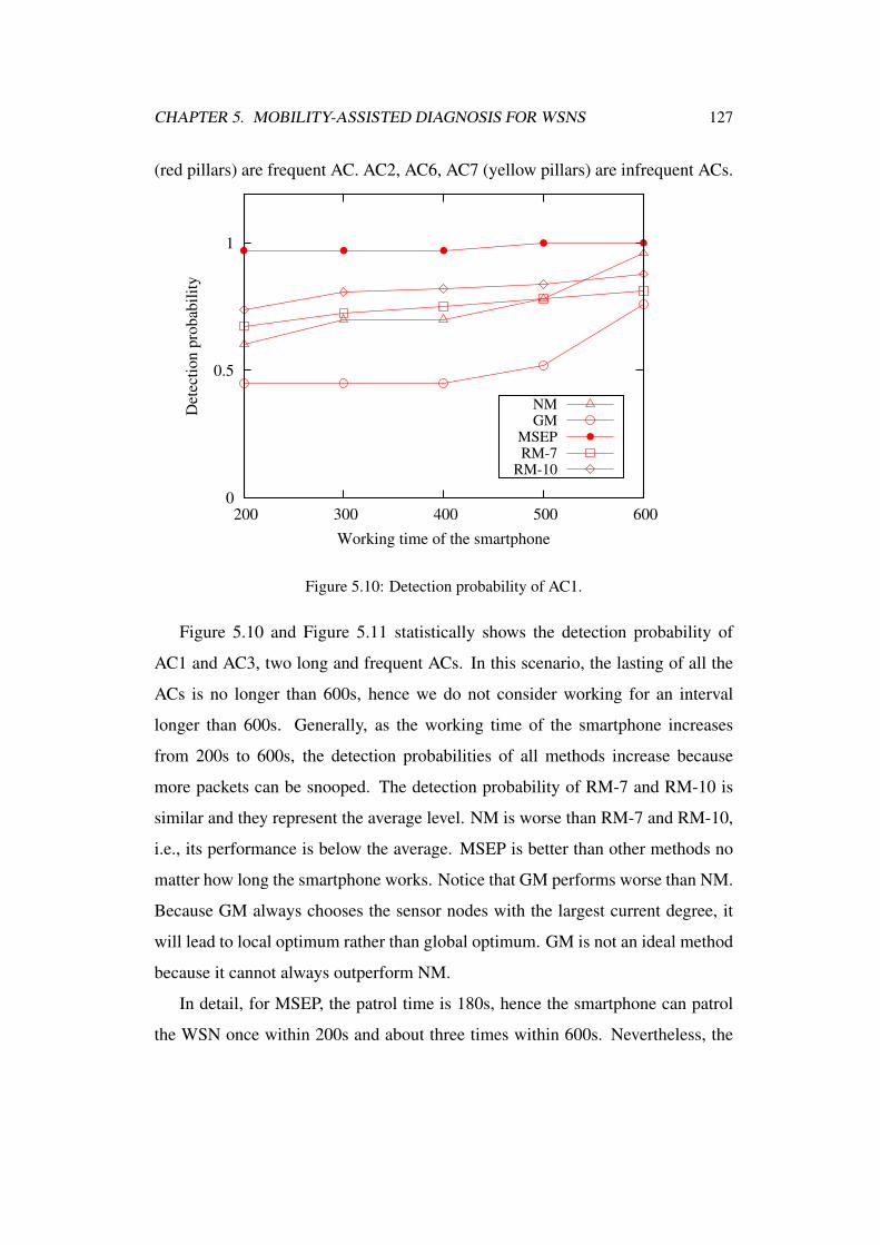
CHAPTER 5. MOBILITY-ASSISTED DIAGNOSIS FOR WSNS 127
(red pillars) are frequent AC. AC2, AC6, AC7 (yellow pillars) are infrequent ACs.
0
0.5
1
200 300 400 500 600
Det
ecti
on
pro
bab
ilit
y
Working time of the smartphone
NMGM
MSEPRM-7
RM-10
Figure 5.10: Detection probability of AC1.
Figure 5.10 and Figure 5.11 statistically shows the detection probability of
AC1 and AC3, two long and frequent ACs. In this scenario, the lasting of all the
ACs is no longer than 600s, hence we do not consider working for an interval
longer than 600s. Generally, as the working time of the smartphone increases
from 200s to 600s, the detection probabilities of all methods increase because
more packets can be snooped. The detection probability of RM-7 and RM-10 is
similar and they represent the average level. NM is worse than RM-7 and RM-10,
i.e., its performance is below the average. MSEP is better than other methods no
matter how long the smartphone works. Notice that GM performs worse than NM.
Because GM always chooses the sensor nodes with the largest current degree, it
will lead to local optimum rather than global optimum. GM is not an ideal method
because it cannot always outperform NM.
In detail, for MSEP, the patrol time is 180s, hence the smartphone can patrol
the WSN once within 200s and about three times within 600s. Nevertheless, the

CHAPTER 5. MOBILITY-ASSISTED DIAGNOSIS FOR WSNS 128
0
0.5
1
200 300 400 500 600
Det
ecti
on
pro
bab
ilit
y
Working time of the smartphone
NMGM
MSEPRM-7
RM-10
Figure 5.11: Detection probability of AC3.
patrol time of NM is 625s, and hence NM can only patrol all the sensor nodes for
about 1 time within 600s. This results in a much lower detection probability of
NM than MSEP when the working time of the smartphone is 200s. So do GM,
RM-7, and RM-10. When the working time is 600s, all the methods can patrol the
WSN for at least 1 time. Because AC1 and AC3 are long and frequent, they are
easy to be discovered by all the methods with high probability. Compared with
other methods, MSEP can save the working time a lot while still maintaining high
detection probability.
Figure 5.12 plots the detection probability of AC2. Since AC2 is infrequent,
the detection probability of AC2 is much lower than those of AC1 and AC3,
especially when the smartphone working time is less than 500s. Specifically, when
the smartphone working time is less than 400s, all methods can hardly collect
enough packets to detect AC2. Generally, the detection probabilities of all the
other methods are lower than that of MSEP. Unlike the case of AC1 and AC3, in
the case of AC2, GM performs better than NM though it is still below RM-7 and
CHAPTER 5. MOBILITY-ASSISTED DIAGNOSIS FOR WSNS 129
0
0.5
1
200 300 400 500 600
Det
ecti
on
pro
bab
ilit
y
Working time of the smartphone
NMGM
MSEPRM-7
RM-10
Figure 5.12: Detection probability of AC2.
RM-10.
Figure 5.13 statistically shows the detection probabilities of AC4, AC5, AC6,
and AC7. The working time is 200s because they are short AC lasting for about
200s. Since AC4 is more frequent than AC5, the detection probability of AC4 is
higher than that of AC5. AC6 and AC7 are infrequent ACs while AC4 and AC5
are frequent ACs, hence the detection probabilities of AC6 and AC7 are lower
than those of AC4 and AC5. For all the short AC, MSEP achieves higher detection
probability than the other methods. GM is better than NM for AC5 and AC6. It
is worse for AC4 and AC7. The performance of RM-7 and RM-10 is similar. GM
and NM are below the average level while MSEP is above the average level.
In summary, Figure 5.14 demonstrates that the detection probability of all
ACs for MSEP is higher than that of all the other methods. In addition, since
more ACs exist, the detection probabilities of all approaches are high when the
smartphone working time approaches 600s. Furthermore, Figure 5.14 shows that
if MSEP is employed, the smartphone only needs to work for about 300s to achieve

CHAPTER 5. MOBILITY-ASSISTED DIAGNOSIS FOR WSNS 130
0
0.5
1
4 5 6 7
Det
ecti
on
pro
bab
ilit
y
Abnormal case number
NMGM
MSEPRM-7
RM-10
Figure 5.13: Detection probability of AC4, AC5, AC6, and AC7 when the working time is
200s.
high detection probability. When the ACs are not as frequent as the ACs in this
experiment, using MSEP to work for a longer time can increase the detection
probability a lot as shown in Figure 5.12. In a word, MSEP can reduce the
smartphone patrol time and increase the failure detection rate.
5.7 Conclusions
In this chapter, we propose a mobility-assisted diagnosis method called MDiag to
diagnosis failures in WSNs with smartphones. The advantages of this approach are
multi-fold: MDiag does not intrude the WSNs and is more efficient than deploying
another network for diagnosis purpose. In addition, MDiag can help the BS find
more failures because it can snoop all kinds of raw packets that are sent out.
Aiming at the targets of all protocol layers, we design statistical rules to guide
the abnormal phenomena determination. MSEP algorithm is further proposed to

CHAPTER 5. MOBILITY-ASSISTED DIAGNOSIS FOR WSNS 131
0
0.5
1
200 300 400 500 600
Det
ecti
on
pro
bab
ilit
y
Working time of the smartphone
NMGM
MSEPRM-7
RM-10
Figure 5.14: Detection probability of all ACs.
improve the detection rate and reduce the patrol time of MDiag. The permanent
failure detection experiments demonstrate that MDiag can help discover more
failures than BS-centralized methods. The experiments on short-term failure
detection show that MSEP algorithm suits WSNs better than NM, GM, and
baseline method RM-K.
2 End of chapter.

Chapter 6
Conclusions
WSN applications facilitate the development in civil, industrial, military, and other
areas. Due to the difference from the traditional networks, including MANETs,
WSNs face new challenges in the development, implementation, and maintenance
of their applications. The contribution of this thesis is to enable successful WSN
applications. In this chapter, we summarize the key research presented in this
thesis, and discuss some future research work.
To assist the development of WSN applications, this thesis proposes a reliable
and efficient MAC protocol for UWASNs. Due to the different transmission
medium used in the water by UWASNs, the efficiency of UWASNs is inferior
to that of the TWSNs. Moreover, the unreliability problem in UWASNs caused by
packet loss is seldom considered. We propose an efficient MAC protocol called
RAS to improve the efficiency in UWASNs. Then RRAS, the reliable RAS, is
implemented to achieve a tradeoff between reliability and efficiency performance
in UWASNs. With information of the rough propagation delays between each node
pair, RAS can arrive at coarse synchronization. Adopting parallel transmissions,
RAS performs priority scheduling. It calculates a compact schedule at the BS
when static routing is applied and the DATA direction is only from the sensor
nodes to the BS. In maintaining the throughput performance, RRAS employs
132
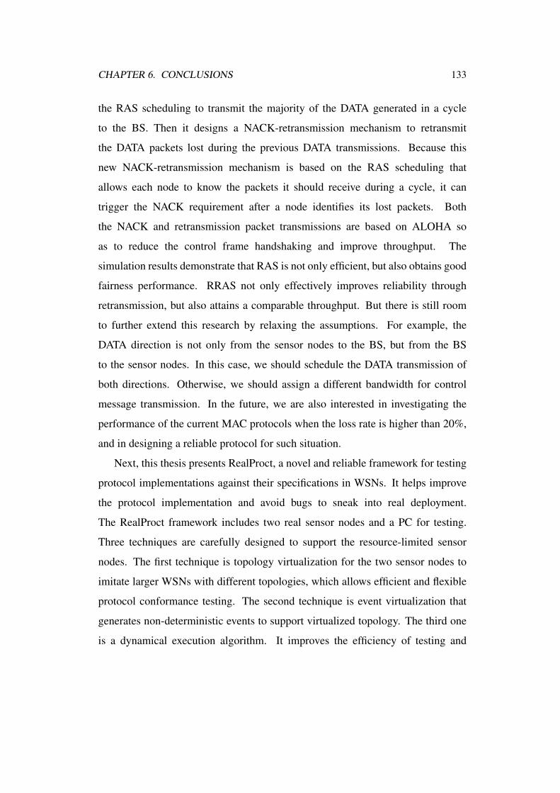
CHAPTER 6. CONCLUSIONS 133
the RAS scheduling to transmit the majority of the DATA generated in a cycle
to the BS. Then it designs a NACK-retransmission mechanism to retransmit
the DATA packets lost during the previous DATA transmissions. Because this
new NACK-retransmission mechanism is based on the RAS scheduling that
allows each node to know the packets it should receive during a cycle, it can
trigger the NACK requirement after a node identifies its lost packets. Both
the NACK and retransmission packet transmissions are based on ALOHA so
as to reduce the control frame handshaking and improve throughput. The
simulation results demonstrate that RAS is not only efficient, but also obtains good
fairness performance. RRAS not only effectively improves reliability through
retransmission, but also attains a comparable throughput. But there is still room
to further extend this research by relaxing the assumptions. For example, the
DATA direction is not only from the sensor nodes to the BS, but from the BS
to the sensor nodes. In this case, we should schedule the DATA transmission of
both directions. Otherwise, we should assign a different bandwidth for control
message transmission. In the future, we are also interested in investigating the
performance of the current MAC protocols when the loss rate is higher than 20%,
and in designing a reliable protocol for such situation.
Next, this thesis presents RealProct, a novel and reliable framework for testing
protocol implementations against their specifications in WSNs. It helps improve
the protocol implementation and avoid bugs to sneak into real deployment.
The RealProct framework includes two real sensor nodes and a PC for testing.
Three techniques are carefully designed to support the resource-limited sensor
nodes. The first technique is topology virtualization for the two sensor nodes to
imitate larger WSNs with different topologies, which allows efficient and flexible
protocol conformance testing. The second technique is event virtualization that
generates non-deterministic events to support virtualized topology. The third one
is a dynamical execution algorithm. It improves the efficiency of testing and
CHAPTER 6. CONCLUSIONS 134
the accuracy of verdict by determining the optimal number of test executions,
while guaranteeing an acceptable probability of false negative and false positive
errors. We implemented RealProct in real sensor nodes and tested the protocol
implementation of the µIP TCP/IP stack in Contiki-2.4. RealProct effectively
found two new bugs and all the previously detected bugs in the µIP TCP/IP stack.
The experiments demonstrated that our protocol conformance testing setup can
effectively detect bugs that might be missing in simulations. We also tested and
validated the protocol implementation of Rime mesh routing in Contiki-2.4. The
results indicated that RealProct can provide a cost-effective and flexible solution
for testing different advanced protocols, like multi-hop routing, which are more
sensitive to the network topology and the non-deterministic events in real wireless
channels.
Due to the limited number of real sensor nodes used, there are some cases that
RealProct cannot virtualize with high similarity. For example, it cannot virtualize
the wireless environment when interference caused by simultaneous transmissions
happens, although the result of interference is easy to be virtualized as packet loss
or erroneous packet. In the future, we will attempt to solve the problem with more
real sensor nodes. In this situation, the control of multiple sensor nodes becomes
difficult. First, synchronization should be achieved so as to maintain the temporal
order of interactions. Second, communications among them need to be solved.
Finally, this thesis proposes MDiag, a Mobility-assisted Diagnosis approach
that employs smartphones to patrol the WSNs and diagnose their failures in
real-time. MDiag can help detecting failures in the WSN protocols after
deployment in real-time, thus facilitating the maintenance. Diagnosing with a
smartphone which is not a component of WSNs does not intrude the execution of
the WSNs. MDiag is more efficient than deploying another network for diagnosis
purpose. In addition, it can help the BS find more failures because it can snoop
all kinds of raw packets that are sent out. Aiming at the targets of all protocol
CHAPTER 6. CONCLUSIONS 135
layers, we design statistical rules to guide the abnormal phenomena determination.
A patrol approach MSEP is further proposed to improve the detection rate and
reduce the patrol time of MDiag. The permanent failure detection experiments
demonstrate that MDiag can help discover more failures than BS-centralized
methods. The experiments on short-term failure detection show that MSEP
algorithm is better than the naive method, greedy method, and baseline method in
increasing the detection rate and reducing the patrol time. Since we do not consider
the traveling cost in our patrol algorithm design, we can take it into account and
give more accurate and effective patrol algorithms in the future. Moreover, we are
also interested in patrolling the deployed WSNs with more than one smartphones.
In conclusion, this thesis investigates the methodologies to enable dependable
WSNs in the aspects of protocol design, testing and diagnosis. Both simulations
and real experiments are conducted to prove the effectiveness of the methods.
Considering that each sensor node is identified by an address and contains
information sensed by the sensors, if we equip any object with the sensors and
mark it with an identity, then we can form the Internet of things (IoT), which
is foreseen to be the next generation of Internet [27]. As WSNs can collect
surrounding context and environment information, they will be the eyes, ears, nose
and even skin of the IoT. Meanwhile, WSN will also get strong support from IoT,
such as cloud computation. In the future, we are interested in integrating the WSN
into the Internet to facilitate a mighty IoT that can monitor and control every corner
of the world.
2 End of chapter.

Bibliography
[1] Crossbow product overview. http://bullseye.xbow.com:81/
Products/wproductsoverview.aspx.
[2] Gloabal mobile phone statistics. http://mobithinking.com/
mobile-marketing-tools/latest-mobile-stats.
[3] The network simulator version 3. http://www.isi.edu/nsnam/
ns/.
[4] The smart dust project. http://robotics.eecs.berkeley.edu/
˜pister/SmartDust/.
[5] Information technology, open systems interconnect, conformance testing
methodology and framework., 1991.
[6] MNP: Multihop network reprogramming service for sensor networks. 2004.
[7] IEEE standard for information technology - telecommunications and
information exchange between systems - local and metropolitan area
networks - specific requirements - part 11: Wireless lan medium access
control (MAC) and physical layer (PHY) specifications, 2007.
[8] Agilent. Agilent 6430 WiMAX: Protocol Conformance Test (PCT) and
Development System. http://cp.literature.agilent.com/
litweb/pdf/5989{-}7513EN.pdf.
136

BIBLIOGRAPHY 137
[9] J. Ahn and B. Krishnamachari. Performance of a propagation delay tolerant
ALOHA protocol for underwater wireless networks. In Proc. of the IEEE
International Conference on Distributed Computing in Sensor Systems, Sep
2008.
[10] I. Akyildiz, W. Su, Y. Sankarasubramaniam, and E. Cayirci. Wireless sensor
networks: a survey. Computer Networks, 38:393–422, 2002.
[11] I. F. Akyildiz, C. D. Pompili, and T. Melodia. Underwater acoustic sensor
networks: Research challenges. Ad Hoc Networks, 3(3):257–279, May
2005.
[12] J. N. Al-Karaki and A. E. Kamal. Routing techniques in wireless
sensor networks: A survey. IEEE Wireless Communications, 11(6):6–28,
December 2004.
[13] G. W. Allen, K. Lorincz, J. Johnson, J. Lees, and M. Welsh. Fidelity
and yield in a volcano monitoring sensor network. In Proc. of the 6th
USENIX Symposium on Operating Systems Design and Implementation,
pages 381–369, Seattle, USA, 2006.
[14] Anritsu. Protocol Conformance Testing of 3G Terminals.
http://www.eu.anritsu.com/news/default.php?id=718.
[15] G. Barrenetxea, F. Ingelrest, G. Schaefer, and M. Vetterli. The hitchhiker’s
guide to successful wireless sensor network deployments. In Proc. of
the 6th International Conference on Embedded Networked Sensor Systems
(SenSys), pages 43–56, 2008.
[16] B. Benson, Y. Li, R. Kastner, B.Faunce, K. Domond, D. Kimball, and
C. Schurgers. Design of a low-cost, underwater acoustic modem for
short-range sensor networks. In Proc. of the IEEE OCEANS Conference,
2010.

BIBLIOGRAPHY 138
[17] S. Bhatti, J. Carlson, H. Dai, J. Deng, J. Rose, A. Sheth, B. Shucker,
C. Gruenwald, A. Torgerson, and R. Han. Mantis os: An embedded
multithreaded operating system for wireless micro sensor platforms. Mobile
Networks and Applications, 10(4), August 2005.
[18] S. Bishop, M. Fairbairn, M. Norrish, P. Sewell, M. Smith, and
K. Wansbrough. Rigorous specification and conformance testing techniques
for network protocols, as applied to TCP, UDP, and Sockets. In Proc.
of ACM Conference on Computer Communication (SIGCOMM), pages
265–276, 2005.
[19] H. Bret, J. Kyle, and B. Hari. Mitigating congestion in wireless sensor
networks. In Proc. of the 2nd International Conference on Embedded
Networked Sensor Systems (SenSys), pages 134–147, 2004.
[20] M. Buettner, G. Yee, E. Anderson, and R. Han. X-mac: A short preamble
mac protocol for duty-cycled wireless sensor networks. In Proc. of the
4th International Conference on Embedded Networked Sensor Systems
(SenSys), 2006.
[21] C. Cadar, D. Dunbar, and D. Engler. KLEE: Unassisted and automatic
generation of high-coverage tests for complex systems programs. In
Proc. of the 8th USENIX Symposium on Operating Systems Design and
Implementation, pages 209–224, 2008.
[22] Q. Cao, T. Abdelzaher, J. Stankovic, and T. He. The LiteOS operating
system: Towards unix-like abstractions for wireless sensor networks.
In Proc. of the ACM/IEEE International Conference on Information
Processing in Sensor Networks (IPSN), 2008.
[23] Q. Cao, T. Abdelzaher, J. Stankovic, K. Whitehouse, and L. Luo.
Declarative tracepoints: A programmable and application independent
BIBLIOGRAPHY 139
debugging system for wireless sensor networks. In Proc. of the
6th International Conference on Embedded Networked Sensor Systems
(SenSys), 2008.
[24] V. G. Cerf and R. E. Kahn. A protocol for packet network
intercommunication. IEEE Transactions on Communications, 22:637–648,
1974.
[25] Y. Chen, O. Gnawali, and M. Kazandjieva. Surviving sensor network
software faults. In Proc. of the 22nd ACM Symposium on Operating Systems
Principles, pages 235–246, 2009.
[26] N. Chirdchoo, W.-S. Soh, and K. C. Chua. Aloha-based MAC protocols
with collision avoidance for underwater acoustic networks. In Proc.
of the IEEE International Conference on Computer Communications
(INFOCOM), pages 1567–1576, June 2007.
[27] D. Christin, A. Reinhardt, P. S. Mogre, and R. Steinmetz. Wireless sensor
networks and the internet of things: Selected challenges. In Proc. of the 8th
GI/ITG KuVS Fachgesprach ”Drahtlose Sensornetze”, 2009.
[28] N. Cooprider, W. Archer, E. Eide, D. Gay, and J. Regehr. Efficient
memory safety for TinyOS. In Proc. of the 5th International Conference
on Embedded Networked Sensor Systems (SenSys), pages 266–279, 2007.
[29] V. Dam, Tijs, Langendoen, and Koen. An adaptive energy-efficient MAC
protocol for wireless sensor networks. In Proc. of the 1st International
Conference on Embedded Networked Sensor Systems (SenSys), pages
171–180, New York, NY, USA, 2003. ACM.
[30] J. Degesys, I. Rose, A. Patel, and R. Nagpal. DESYNC: Self-organizing
desynchronization and TDMA on wireless sensor networks. In Proc. of the

BIBLIOGRAPHY 140
International Conference on Information Processing in Sensor Networks
(IPSN), 2007.
[31] J. Deng, B. Liang, and P. Varshney. Tuning the carrier sensing range of
IEEE 802.11 MAC. In Proc. of the Global Telecommunications Conference
(GLOBECOM), pages 2987–2991, 2004.
[32] A. Dunkels. Full tcp/ip for 8 bit architectures. In Proc. of the 1st
ACM/USENIX International Conference on Mobile Systems, Applications
and Services (MobiSys), pages 85–98, 2003.
[33] A. Dunkels, B. Gronvall, and T. Voigt. Contiki - a lightweight and flexible
operating system for tiny networked sensors. In Proc. of the 29th Annual
IEEE International Conference on Local Computer Networks (LCN), 2004.
[34] A. Dunkels, T. Voigt, and J. Alonso. Making TCP/IP viable for wireless
sensor networks. In Proc. of the 1st European Workshop on Wireless Sensor
Networks (EWSN), Berlin, Germany, 2004.
[35] A. Dunkels, T. Voigt, J. Alonso, H. Ritter, and J. Schiller. Connecting
wireless sensornets with TCP/IP networks. In Proc. of the 2nd International
Conference on Wired/Wireless Internet Communications (WWIC), pages
583–594, 2004.
[36] A. El-Hoiydi and J.-D. Decotignie. WiseMAC: An ultra low power mac
protocol for the downlink of infrastructurewireless sensor networks. In
Proc. of the 9th IEEE Symposium on Computers and Communication
(ISCC), Alexandria, Egypt, June 2004.
[37] J. Elson and K. Romer. Wireless sensor networks: a new regime for
time synchronization. SIGCOMM Computer Communincation Review,
33(1):149–154, 2003.
BIBLIOGRAPHY 141
[38] J. Eriksson, F. Osterlind, N. Finne, N. Tsiftes, A. Dunkels, T. Voigt,
R. Sauter, and P. J. Marron. Towards interoperability testing for wireless
sensor networks with cooja/mspsim. In Proc. of the 6th European
Conference on Wireless Sensor Networks (EWSN), Cork, Ireland, February
2009.
[39] L. Freitag, M. Grund, S. Singh, J. Partan, P. Koski, and K. Ball. The
WHOI micro-modem: An acoustic communications and navigation system
for multiple platforms. In Proc. of the IEEE OCEANS Conference, 2005.
[40] F.Schill, U.R.Zimmer, and J.Trumpf. Visible spectrum optical
communication and distance sensing for underwater applications. In Proc.
of Australasian Conference Robotics and Automation, 2004.
[41] A. Ghosh and S. K. Das. Coverage and connectivity issues in wireless sensor
networks: A survey. Pervasive and Mobile Computing, 4:303–334, 2008.
[42] O. Gnawali, R. Fonseca, K. Jamieson, D. Moss, and P. Levis. Collection
tree protocol. In Proc. of the 7th International Conference on Embedded
Networked Sensor Systems (SenSys), 2009.
[43] X. Guo, M. R. Frater, and M. J. Ryan. A propagation-delay-tolerant
collision avoidance protocol for underwater acoustic sensor networks. In
Proc. of the IEEE OCEANS Conference, September 2006.
[44] X. Guo, M. R. Frater, and M. J. Ryan. An adaptive
propagation-delay-tolerant MAC protocol for underwater acoustic sensor
networks. In Proc. of the IEEE OCEANS Conference, pages 1–5, 2007.
[45] B. Hailpern and P. Santhanam. Software debugging, testing, and
verification. IBM Systems Journal, 41:4–12, 2001.
BIBLIOGRAPHY 142
[46] G. Halkes, T. V. Dam, and K. Langendoen. Comparing energy-saving MAC
protocols for wireless sensor networks. Mobile Networks and Applications,
10(5):783–791, 2005.
[47] W. R. Heinzelman, A. Chandrakasan, and H. Balakrishnan. Energy-efficient
communication protocol for wireless microsensor networks. In Proc. of the
33rd Hawaii International Conference on System Sciences, January 2000.
[48] J. Heo, B. Gu, and S. I. Eo. Energy efficient program updating for sensor
nodes with flash memory. In Proc. of the 2010 ACM Symposium on Applied
Computing, 2010.
[49] J. Hill, R. Szewczyk, A. Woo, S. Hollar, D. Culler, and K. Pister.
System architecture directions for networked sensors. In Proc. of the
9th International Conference on Architectural Support for Programming
Languages and Operating Systems, Cambridge, MA, 2000.
[50] J. W. Hui and D. Culler. The dynamic behavior of a data dissemination
protocol for network programming at scale. In Proc. of the 2nd International
Conference on Embedded Networked Sensor Systems (SenSys), pages
266–279, 2004.
[51] C. Intanagonwiwat, R. Govindan, D. Estrin, J. Heidemann, , and F. Silva.
Directed diffusion for wireless sensor networking. IEEE/ACM Transactions
on Networking, 11(1):2–16, 2003.
[52] J. Jeong and D. Culler. Incremental network programming for wireless
sensors. In Proc. of the IEEE Communications Society Conference on
Sensor, Mesh and Ad Hoc Communications and Networks (SECON), pages
25–33, 2004.
[53] X. Ji and H. Zha. Sensor positioning in wireless ad-hoc sensor networks
using multidimensional scaling. In Proc. of the IEEE International

BIBLIOGRAPHY 143
Conference on Computer Communications (INFOCOM), pages 2652–2661,
2004.
[54] D. S. Johnson. Approximation algorithms for combinatorial problems. In
Proc. of the 5th Annual ACM Symposium on Theory of Computing, 1973.
[55] R. M. Karp. Reducibility Among Combinatorial Problems. 1972.
[56] M. M. H. Khan, T. Abdelzaher, and K. K. Gupta. Towards diagnostic
simulation in sensor networks. In Proc. of the 4th IEEE International
Conference on Distributed Computing in Sensor Systems (ICDCS), pages
252–265, 2008.
[57] M. M. H. Khan, H. K. Le, H. Ahmadi, T. F. Abdelzaher, and
J. Han. Dustminer: Troubleshooting interactive complexity bugs in sensor
networks. In Proc. of the 6th International Conference on Embedded
Networked Sensor Systems (SenSys), pages 99–112, 2008.
[58] M. M. H. Khan, L. Luo, C. Huang, and T. Abdelzaher. SNTS:
Sensor network troubleshooting suite. In Proc. of the IEEE International
Conference on Distributed Computing in Sensor Systems (DCOSS), 2007.
[59] C. Killian, J. W. Anderson, R. Jhala, and A. Vahdat. Life, death, and
the critical transition: Finding liveness bugs in systems code. In Proc. of
4th USENIX Symposium on Networked Systems Design & Implementation
(NSDI), pages 243–256, 2007.
[60] Kim, Youngmin, Shin, Hyojeong, Cha, and Hojung. A multi-channel
MAC implementation for wireless sensor networks. In Proc. of the
5th International Conference on Embedded Networked Sensor Systems
(SenSys), pages 371–372, New York, NY, USA, 2007. ACM.
[61] J. C. King. Symbolic execution and program testing. Communications of
the ACM, 19(7):385–394, 1976.

BIBLIOGRAPHY 144
[62] K. Klues, C.-J. M. Liang, J. Paek, R. M. aloiu E, P. Levis, A. Terzis,
and R. Govindan. TOSThreads: Thread-safe and non-invasive preemption
in tinyos. In Proc. of the 7th International Conference on Embedded
Networked Sensor Systems (SenSys), pages 266–279, 2009.
[63] N. Kothari, T. Millstein, and R. Govindan. Deriving state machines from
TinyOS programs using symbolic execution. In Proc. of the 7th ACM/IEEE
International Conference on Information Processing in Sensor Networks
(IPSN), pages 271–282, 2008.
[64] N. Kothari, K. Nagaraja, V. Raghunathan, F. Sultan, and S. Chakradhar.
HERMES: A software architecture for visibility and control in wireless
sensor network deployments. In Proc. of the 7th ACM/IEEE International
Conference on Information Processing in Sensor Networks (IPSN), pages
395–406, 2008.
[65] V. Krunic, E. Trumpler, and R. Han. NodeMD: Diagnosing node-level
faults in remote wireless sensor systems. In Proc. of the 5th International
Conference onMobile Systems, Applications, and Services (Mobisys), pages
43–56, June 2007.
[66] K. Langendoen, A. Baggio, and O. Visser. Murphy loves potatoes:
Experiences from a pilot sensor network deployment in precision
agriculture. In Proc. of the International Workshop on Parallel and
Distributed Real-Time Systems, April 2006.
[67] P. Levis. Tinyos programming. http://csl.stanford.edu/ pal/pubs/tinyos-programming.pdf.
[68] P. Levis, N. Lee, M. Welsh, and D. Culler. TOSSIM: Accurate and scalable
simulation of entire tinyos applications. In Proc. of the 1st International
Conference on Embedded Networked Sensor Systems (SenSys), pages
266–279, 2003.

BIBLIOGRAPHY 145
[69] P. Levis, S. Madden, J. Polastre, R. Szewczyk, A. Woo, D. Gay, J. Hill,
M. Welsh, E. Brewer, and D. Culler. TinyOS: An operating system for
sensor networks. Ambient Intelligence, pages 115–148, 2005.
[70] P. Levis, N. Patel, D. Culler, and S. Shenker. Trickle: A self-regulating
algorithm for code propagation and maintenance in wireless sensor
networks. In Proc. of the 1st Symposium on Networked Systems Design
and Implementation (NSDI), pages 15–28, 2004.
[71] J. Li, J. Jannotti, D. D. Couto, D. Karger, and R. Morris. A scalable location
service for geographic ad-hoc routing. In Proc. of the 6th ACM International
Conference on Mobile Computing and Networking (MobiCom), pages
120–130, 2000.
[72] P. Li and J. Regehr. T-Check: Bug finding for sensor networks. In Proc. of
the 9th ACM/IEEE International Conference on Information Processing in
Sensor Networks (IPSN), pages 174–185, 2010.
[73] W. Li and J. Han. Dynamic wireless sensor network parameters
optimization adapting different node mobility. In Proc. of the IEEE
Aerospace Conference, 2010.
[74] B. Liu, P. Brass, and O. Dousse. Mobility improves coverage of sensor
networks. In Proc. of the 6th International Symposium on Mobile Ad Hoc
Networking and Computing (MobiHoc), 2005.
[75] K. Liu, M. Li, Y. Liu, M. Li, Z. Guo, and F. Hong. Passive diagnosis for
wireless sensor networks. In Proc. of the 6th International Conference on
Embedded Networked Sensor Systems (SenSys), pages 1132–1144, 2008.
[76] K. Liu, Q. Ma, X. Zhao, and Y. Liu. Self-diagnosis for large scale wireless
sensor networks. In Proc. of the 30th IEEE International Conference on
Computer Communications (INFOCOM), 2011.
BIBLIOGRAPHY 146
[77] L. Luo, T. He, G. Zhou, L. Gu, T. F. Abdelzaher, and J. A. Stankovic.
Achieving repeatability of asynchronous events in wireless sensor networks
with envirolog. In Proc. of the 25th IEEE International Conference on
Computer Communications (INFOCOM), 2006.
[78] D. J. Malan, M. Welsh, and M. D. Smith. A public-key infrastructure for
key distribution in tinyos based on elliptic curve cryptography. In Proc.
of the IEEE Communications Society Conference on Sensor and Ad Hoc
Communications and Networks (SECON), pages 71–80, 2004.
[79] G. Mao, B. Fidan, and B. D. Anderson. Wireless sensor network localization
techniques. Computer Networks, 51:2529–2553, 2007.
[80] M. Maroti, Branislav, Simon, G. Simon, and A. Ledeczi. The flooding time
synchronization protocol. In Proc. of the 2th International Conference on
Embedded Networked Sensor Systems (SenSys)f, pages 39–49, New York,
NY, USA, 2004. ACM.
[81] X. Miao, K. Liu, Y. He, Y. Liu, and D. Papadias. Agnostic diagnosis:
Discovering silent failures in wireless sensor networks. In Proc. of
the 30th IEEE International Conference on Computer Communications
(INFOCOM), 2011.
[82] M. Molins and M. Stojanovic. Slotted FAMA: a MAC protocol for
underwater acoustic networks. In Proc. of the IEEE OCEANS Conference,
2006.
[83] J. Neyman and E. S. Pearson. On the problem of the most efficient tests of
statistical hypotheses. Royal Society of London Philosophical Transactions
Series A, 231:289–337, 1933.
[84] E. C.-H. Ngai, H. Huang, J. Liu, and M. B. Srivastava. Oppsense:
Information sharing for mobile phones in sensing field with data

BIBLIOGRAPHY 147
repositories. In Proc. of the IEEE Communications Society Conference on
Sensor, Mesh and Ad Hoc Communications and Networks (SECON), 2011.
[85] F. Osterlind, A. Dunkels, J. Eriksson, N. Finne, and T. Voigt. Cross-level
sensor network simulation with cooja. In Proc. of the First IEEE
International Workshop on Practical Issues in Building Sensor Network
Applications (SenseApp 2006), 2006.
[86] J. Partan, J. Kurose, and B. N. Levine. A survey of practical issues in
underwater networks. In Proc. of the 1st ACM International Workshop on
Underwater Networks, pages 17–24, Sep 2006.
[87] B. Peleato and M. Stojanovic. A mac protocol for ad-hoc underwater
acoustic sensor networks. In Proc. of the 1st ACM International Workshop
on Underwater Networks, pages 113–115, Sep 2006.
[88] J. Polastre, J. Hill, and D. Culler. Versatile low power media access for
wireless sensor networks. In Proc. of the 2th International Conference on
Embedded Networked Sensor Systems (SenSys), 2004.
[89] J. Polley, D. Blazakis, J. McGee, D. Rusk, and J. S. Baras. ATEMU:
A fine-grained sensor network simulator. In Proc. of the 1st IEEE
Communications Society Conference on Sensor, Mesh and Ad Hoc
Communications and Networks, pages 145–152, 2004.
[90] J. J. X. J. Prabal Dutta, Jay Taneja and D. Culler. A building block approach
to sensornet systems. In Proc. of the 6th International Conference on
Embedded Networked Sensor Systems (SenSys), 2008.
[91] S. T. B. practices. Software testing best practices. Technical Report RC
21457, Center for Software Engineering, IBM Research, 1999.
BIBLIOGRAPHY 148
[92] J. Preisig. Acoustic propagation considerations for underwater acoustic
communications network development. In Proc. of the 1st ACM
International Workshop on Underwater Networks, pages 1–5, Sep 2006.
[93] N. B. Priyantha, A. Kansal, M. Goraczko, and F. Zhao. Tiny web services:
Design and implementation of interoperable and evolvable sensor networks.
In Proc. of the 6th International Conference on Embedded Networked
Sensor Systems (SenSys), 2008.
[94] M. A. Rahman, A. E. Saddik, and W. Gueaieb. Wireless sensor network
transport layer: State of the art. In S. C. Mukhopadhyay and Y. M.
Huang, editors, Sensors: Advancements in Modeling, Design Issues,
Fabrication and Practical Applications, volume 21, chapter 3, pages
221–245. Springer-Verlag, 2008.
[95] N. Ramanathan, K. Chang, R. Kapur, L. Girod, E. Kohler, and D. Estrin.
Sympathy for the sensor network debugger. In Proc. of the 3rd International
Conference on Embedded Networked Sensor Systems (SenSys), pages
255–267, 2005.
[96] S. Ray, W. Lait, and I. C. Paschalidisl. Deployment optimization of
sensornet-based stochastic location-detection systems. In Proc. of the IEEE
International Conference on Computer Communications (INFOCOM),
volume 4, pages 2279–2289, March 2005.
[97] O. Rensfelt, F. Hermans, L.-A. Larzon, and P. Gunningberg. Sensei-uu: A
relocatable sensor network testbed. In Proc. of the 5th ACM International
workshop on Wireless Network Testbeds, Experimental Evaluation and
Characterization, 2010.
[98] P. Reynolds, C. Killian, J. L. Wiener, J. C. Mogul, M. A. Shah, and
A. Vahdat. Pip: Detecting the unexpected in distributed systems. In Proc.

BIBLIOGRAPHY 149
of the 3rd Symposium on Networked Systems Design and Implementation
(NSDI), 2006.
[99] I. Rhee, A. Warrier, M. Aia, and J. Min. Z-mac: a hybrid MAC for wireless
sensor networks. In Proc. of the 3rd International Conference on Embedded
Networked Sensor Systems (SenSys), pages 90–101, Nov 2005.
[100] M. Ringwald, K. Romer, and A. Vitaletti. Passive inspection of sensor
networks. In Proc. of the IEEE International Conference on Distributed
Computing in Sensor Systems (DCOSS), 2007.
[101] K. Romer and J. Ma. PDA: Passive distributed assertions for sensor
networks. In Proc. of the 8th ACM/IEEE International Conference on
Information Processing in Sensor Networks (IPSN), pages 337–348, 2009.
[102] R. Sasnauskas, O. Landsiedel, M. H. Alizai, C. Weisez, S. Kowalewskiz,
and K. Wehrle. KleeNet: Discovering insidious interaction bugs in wireless
sensor networks before deployment. In Proc. of the 9th ACM/IEEE
International Conference on Information Processing in Sensor Networks
(IPSN), pages 186–196, 2010.
[103] C. Schurgers, O. Aberthorne, and M. B. Srivastava. Modulation scaling
for energy aware communication systems. In Proc. of the International
Symposium on Low Power Electronics and Design (ISLPED), 2001.
[104] J. Sen. A survey on wireless sensor network security. International Journal
of Communication Networks and Information Security, 1(2):55–78, August
2009.
[105] S. Shahabudeen and M. Motani. Performance analysis of a MACA
based protocol for adhoc underwater networks. In Proc. of the 4th ACM
International Workshop on Underwater Networks, Sep 2009.
BIBLIOGRAPHY 150
[106] Y. Shi and Y. T. Hou. Theoretical results on base station movement problem
for sensor network. In Proc. of the IEEE International Conference on
Computer Communications (INFOCOM), 2008.
[107] E. Shih, S.-H. Cho, N. Ickes, R. Min, A. Sinha, A. Wang, and
A. Chandrakasan. Physical layer driven protocol and algorithm design
for energy-efficient wireless sensor networks. In Proc. of the 7th Annual
International Conference on Mobile Computing and Networking, pages
272–287, 2001.
[108] N. Soreide, C. Woody, and S. Holt. Overview of ocean based buoys
and drifters: Present applications and future needs. In Proc. of the
16th International Conference on Interactive Information and Processing
Systems (IIPS) for Meteorology, Oceanography, and Hydrology, Jan 2004.
[109] E. Soroush, K. Wu, and J. Pei. Fast and quality-guaranteed data streaming
in resource-constrained sensor networks. In Proc. of the 9th ACM
International Symposium on Mobile Ad Hoc Networking and Computing,
2008.
[110] F. Stajano. Security for Ubiquitous Computing. Wiley, 2002.
[111] T. Stathopoulos, D. McIntire, and W. J. Kaiser. The energy endoscope:
Real-time detailed energy accounting for wireless sensor nodes. In Proc. of
the International Conference on Information Processing in Sensor Networks
(IPSN), 2008.
[112] Y. Sunhee and S. Cyrus. The clustered aggregation (CAG) technique
leveraging spatial and temporal correlations in wireless sensor networks.
ACM Transactions on Sensor Networks, 3(1):3, March 2007.

BIBLIOGRAPHY 151
[113] A. A. Syed and J. Heidemann. Time synchronization for high latency
acoustic networks. In Proc. of the IEEE International Conference on
Computer Communications (INFOCOM), 2006.
[114] A. A. Syed, W. Ye, and J. Heidemann. T-Lohi: A new class of MAC
protocols for underwater acoustic sensor networks. In Proc. of the IEEE
International Conference on Computer Communications (INFOCOM),
pages 789–797, Sep 2008.
[115] R. Szewczyk, E. Osterweil, J. Polastre, M. Hamilton, A. Mainwaring, and
D. Estrin. Habitat monitoring with sensor networks. Communications of the
ACM, 47(6):34–40, 2004.
[116] W. P. Timing and B. L. Titzer. Avrora: Scalable sensor network simulation.
In Proc. of the 9th ACM/IEEE International Conference on Information
Processing in Sensor Networks (IPSN), pages 477–482, 2005.
[117] L. T. Tracy and S. Roy. A reservation MAC protocol for ad-hoc underwater
acoustic sensor networks. In Proc. of the 3st ACM International Workshop
on Underwater Networks, pages 95–98, 2008.
[118] J. Tretmans. An overview of OSI conformance testing, 2001.
[119] C.-Y. Wan, S. B. Eisenman, and A. T. Campbell. CODA: Congestion
detection and avoidance in sensor networks. In Proc. of the 1st International
Conference on Embedded Networked Sensor Systems (SenSys), pages
266–279, 2003.
[120] A. Y. Wang, S. H. Cho, C. G. Sodini, and A. P. Chandrakasan. Energy
efficient modulation and MAC for asymmetric RF microsensor systems. In
Proc. of the International Symposium on Low Power Electronics and Design
(ISLPED), 2001.
BIBLIOGRAPHY 152
[121] Q. Wang, Y. Zhu, and L. Cheng. Reprogramming wireless sensor networks:
challenges and approaches. IEEE Network, 20(3):48–55, June 2006.
[122] X. Wang, G. Xing, Y. Zhang, and C. Lu. Integrated coverage and
connectivity configuration in wireless sensor networks. In Proc. of the 3rd
international conference on Embedded networked sensor systems (SenSys),
2005.
[123] J. Wu, S. Yang, and M. Cardei. On maintaining sensor-actor connectivity
in wireless sensor and actor networks. In Proc. of the IEEE International
Conference on Computer Communications (INFOCOM), 2008.
[124] G. Xing, C. Lu, R. Pless, and Q. Huang. On greedy geographic routing
algorithms in sensing-covered networks. In Proc. of the 5th International
Symposium on Mobile Ad Hoc Networking and Computing (MobiHoc),
pages 31–42, New York, NY, USA, 2004. ACM.
[125] G. Xing, J. Wang, K. Shen, Q. Huang, X. Jia, and H. C. So.
Mobility-assisted spatiotemporal detection in wireless sensor networks. In
Proc. of the International Conference on Distributed Computing System
(ICDCS), pages 784–794, Genova, Italy, June 2008.
[126] G. Xing, T. Wang, W. Jia, and M. Li. Rendezvous design algorithms for
wireless sensor networks with a mobile base station. In Proc. of the 9th
International Symposium on Mobile Ad Hoc Networking and Computing
(MobiHoc), 2008.
[127] J. Xiong, M. R. Lyu, and K.-W. Ng. Mitigate the bottleneck of underwater
acoustic sensor networks via priority scheduling. In Proc. of the 6th
International Conference on Mobile Ad-hoc and Sensor Networks, pages
53–60, 2010.

BIBLIOGRAPHY 153
[128] J. Xiong, M. R. Lyu, and K.-W. Ng. A reliable and efficient mac
protocol for underwater acoustic sensor networks. International Journal
of Distributed Sensor Networks (IJDSN), special issue on Sensor Networks
for High-Confidence Cyber-Physical Systems, October 2011.
[129] J. Xiong, E. C.-H. Ngai, Y. Zhou, and M. R. Lyu. Realproct: Reliable
protocol conformance testing with real nodes forwireless sensor networks.
In The 10th IEEE International Conference on Trust, Security and Privacy
in Computing and Communications, 2011.
[130] N. Xu, S. Rangwala, K. K. Chintalapudi, D. Ganesan, A. Broad,
R. Govindan, and D. Estrin. A wireless sensor network for structural
monitoring. In Proc. of the 2th International Conference on Embedded
Networked Sensor Systems (SenSys), pages 13–24, 2004.
[131] J. Yackoski and C.-C. Shen. Achieving high channel utilization in a
time-based acoustic MAC protocol. In Proc. of the 3th ACM International
Workshop on Underwater Networks, pages 59–66, 2008.
[132] J. Yang, M. L. Soffa, L. Selavo, and K. Whitehouse. Clairvoyant: A
comprehensive source-level debugger for wireless sensor networks. In
Proc. of the 5th International Conference on Embedded Networked Sensor
Systems (SenSys), pages 189–203, 2007.
[133] W. Ye, J. Heidemann, and D. Estrin. An energy-efficient MAC protocol
for wireless sensor networks. In Proc. of the 21th IEEE Conference on
Computer Communications (INFOCOM), pages 1567–1576, June 2002.
[134] S. Yoon, C. Vveerarittiphan, and M. L. Sichitiu. Tiny-sync: Tight time
synchronization for wireless sensor networks. ACM Transactions on Sensor
Networks, 3(2):8, 2007.

BIBLIOGRAPHY 154
[135] Y. Zhou, X. Chen, M. R. Lyu, and J. Liu. Sentomist: Unveiling transient
sensor network bugs via symptom mining. In Proc. of the International
Conference on Distributed Computing System (ICDCS), pages 784–794,
Genova, Italy, June 2010.
[136] Y. Zhou, E. C.-H. Ngai, M. R. Lyu, and J. Liu. A power-controlled real-time
data transport protocol for wireless sensor-actuator networks. In Proc. of
the IEEE Wireless Communications and Networking Conference (WCNC),
2007.
[137] Y. Zhou, J. Xiong, M. R. Lyu, J. Liu, and K.-W. Ng. Energy-efficient
on-demand contour service for wireless sensor networks. In Proc. of the
6nd IEEE International Conference on Mobile Ad-Hoc and Sensor Systems
(MASS), Nov 2009.
[138] S. Zhu, S. Setia, and S. Jajodia. LEAP: Efficient security mechanism
for large-scale distributed sensor networks. ACM Transactions on Sensor
Networks (TOSN), 2(4):500–528, November 2006.